Dynamics as the Boundary of Identifiability

1. Introduction

Newton’s laws have served as the foundation of classical mechanics for over three centuries. The traditional ontological interpretation presents them as fundamental statements about physical reality: the first law postulates inertia, the second establishes the relationship between force, mass, and acceleration, the third declares the equality of action and reaction. It is possible to look at these useful and widely experimentally confirmed statements with less historical baggage of that era and without the irrational aura of sanctity.

It is natural to begin with the simplest descriptive model. This model consists of the system input, which presumably can be influenced, a black box, and the observed output. The task consists of identifying (modeling in the best possible way) the black box. It is assumed that there is the possibility to influence the input and the input causally depends on the output. This is a standard approach within the framework of system identification science.

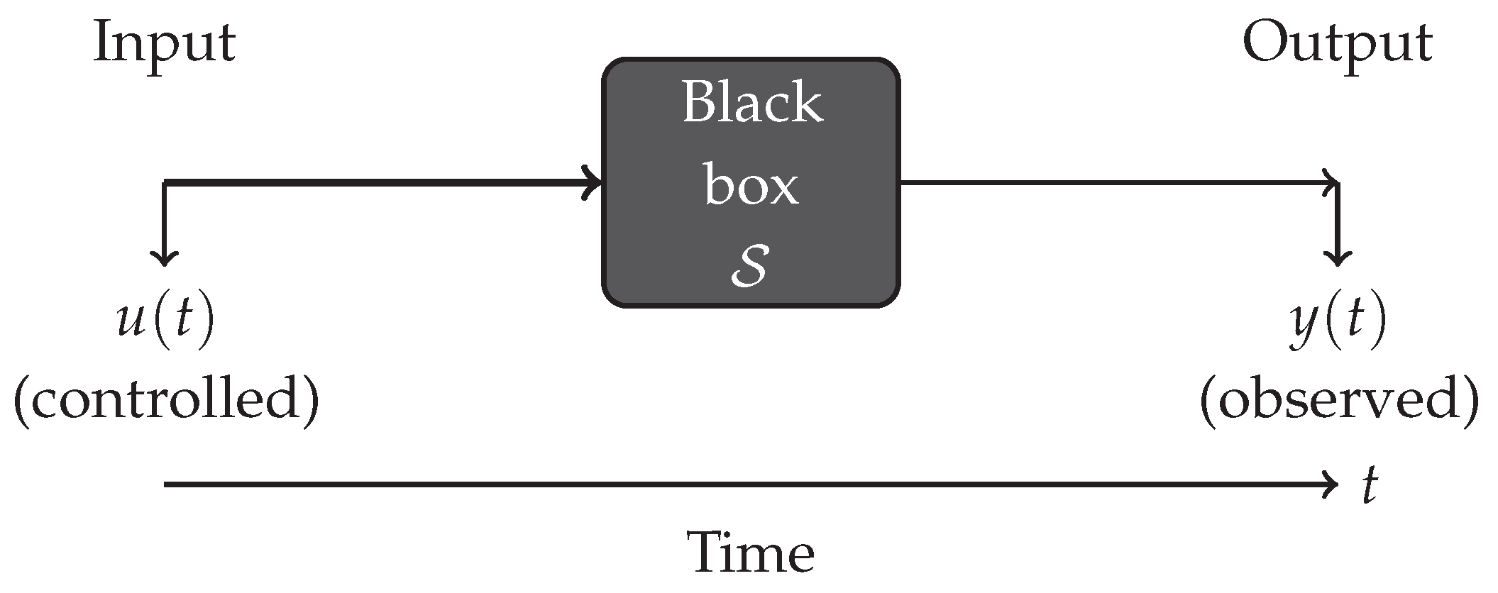
Causality (causality) in this context means that the system output at time moment t depends only on input actions at moments $\tau \le t$, but not on future inputs $\tau >t$. Mathematically, for a linear system with impulse response $g\left(\tau \right)$:

$$y\left(t\right)={\int }_{-\infty }^{t}g(t-\tau )u\left(\tau \right)d\tau$$

(1)

causality is equivalent to the condition $g\left(\tau \right)=0$ for all $\tau <0$. The system cannot “foresee” future inputs.

Strict causality (strict causality) is a stronger requirement: the output at moment t depends only on inputs at moments $\tau <t$ (strictly less), but not on $u\left(t\right)$ at the same moment. This means that $g\left(0\right)=0$, i.e., the system has a delay of at least one time step. In discrete time for a strictly causal system:

$$y\left(t\right)=\sum _{k=1}^{\infty }g\left(k\right)u(t-k)$$

(2)

where summation starts from $k=1$, not from $k=0$.

For second-order mechanical systems ($F=m\ddot{x}$), strict causality is natural: instantaneous change of force does not cause instantaneous change of coordinate or even velocity, since only acceleration changes. The transfer function $G\left(s\right)=1/\left(m{s}^2\right)$ is strictly proper: the degree of the numerator is less than the degree of the denominator, which is equivalent to strict causality.

In the 20th century, system identification theory emerged, which deals with constructing mathematical models of dynamic systems based on experimental observable “input-output” data. The monograph by Ljung [1] represents a good starting point for presenting this theory, establishing standards of mathematical rigor.

The focus of this article is on the question of identifiability as such, in other words, what can be understood in principle at all and where are the boundaries of understandability in this approach.

In the present work, a conceptual inversion of the widespread logic is proposed. Instead of using Newton’s laws as the basis for grey-box modeling, the laws themselves are interpreted as statements about the conditions and boundaries of identifiability. In this epistemological reinterpretation, Newton’s laws become not ontological postulates, but methodological constraints on model recovery from data.

2. Formal Apparatus of System Identification Theory

2.1. Dynamic Systems and Models

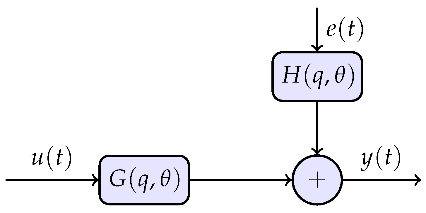
Consider a linear time-invariant system in discrete time:

$$y\left(t\right)=G(q,\theta )u\left(t\right)+H(q,\theta )e\left(t\right)$$

(3)

where $y\left(t\right)$ is the output, $u\left(t\right)$ is the input, $e\left(t\right)$ is white noise, q is the shift operator ($qu\left(t\right)=u(t+1)$), $\theta \in {\mathbb{R}}^d$ is the parameter vector.

In simple words: The transfer function $G(q,\theta )$ describes how the input signal $u\left(t\right)$ (for example, the applied force) is transformed into the output signal $y\left(t\right)$ (for example, the body position). The parameters $\theta$ are the unknown characteristics of the system (mass, spring stiffness, etc.) that need to be determined from experimental data. The term $H(q,\theta )e\left(t\right)$ models measurement noise and random disturbances.

Definition 1 

(Model Structure, Ljung [1], Section 4.2). A model structure $\mathcal{M}$ is a mapping $\mathcal{M}:D_{\mathcal{M}}\to \mathcal{P}$, where $D_{\mathcal{M}}\subset {\mathbb{R}}^d$ is the set of admissible parameters, $\mathcal{P}$ is the set of predictors (forecasting models).

In simple words: A model structure is a family of possible models parameterized by the vector $\theta$. For example, for a mass on a spring, the model structure can be $m\ddot{x}+kx=F\left(t\right)$, where the parameters $\theta =(m,k)$ are the mass and stiffness. Each set $(m,k)$ corresponds to its own model from the family $\mathcal{M}$.

2.2. Identifiability: Can Parameters Be Determined Uniquely?

Definition 2 

(Global Identifiability, Ljung [1], Definition 4.6). A model structure $\mathcal{M}$ is globally identifiable at a point ${\theta }^{*}$ if

$$\mathcal{M}\left(\theta \right)=\mathcal{M}\left({\theta }^{*}\right),\theta \in D_{\mathcal{M}}\Rightarrow \theta ={\theta }^{*}$$

(4)

In simple words: A system is identifiable if the parameters $\theta$ can be uniquely recovered from experimental data $\left\{u\right(t),y(t\left)\right\}$. If two different parameter sets ${\theta }_1\ne {\theta }_2$ lead to identical observed output signals $y\left(t\right)$ for all possible inputs $u\left(t\right)$, then the system is unidentifiable—these parameters can never be distinguished experimentally.

Physical example: Imagine two masses on springs: $(m_1,k_1)$ and $(m_2,k_2)$. If for any excitation $F\left(t\right)$ both systems behave identically (produce the same displacement $x\left(t\right)$), then it is impossible to determine which one is the real one from observations. In this case, the parameters are unidentifiable. For identifiability, different parameter sets must produce distinguishable experimental signatures.

2.3. Persistent Excitement: Richness of Input Signal

Definition 3 

(Data Informativeness, Ljung [1], Definition 8.2). A data set $Z^{\infty }={\{u\left(t\right),y\left(t\right)\}}_{t=1}^{\infty }$ is informative with respect to a model structure $\mathcal{M}$ if for any two distinct models $W_1,W_2\in \mathcal{M}$

$$\overline{E}{[W_1\left(q\right)z\left(t\right)-W_2\left(q\right)z\left(t\right)]}^2=0\Rightarrow W_1\left(e^{i\omega }\right)\equiv W_2\left(e^{i\omega }\right)$$

(5)

In simple words: Data is informative if it allows distinguishing different models within the chosen family $\mathcal{M}$. If two models $W_1$ and $W_2$ give identical predictions for all collected data, then either these models are truly identical, or the data is not rich enough to distinguish them.

Definition 4 

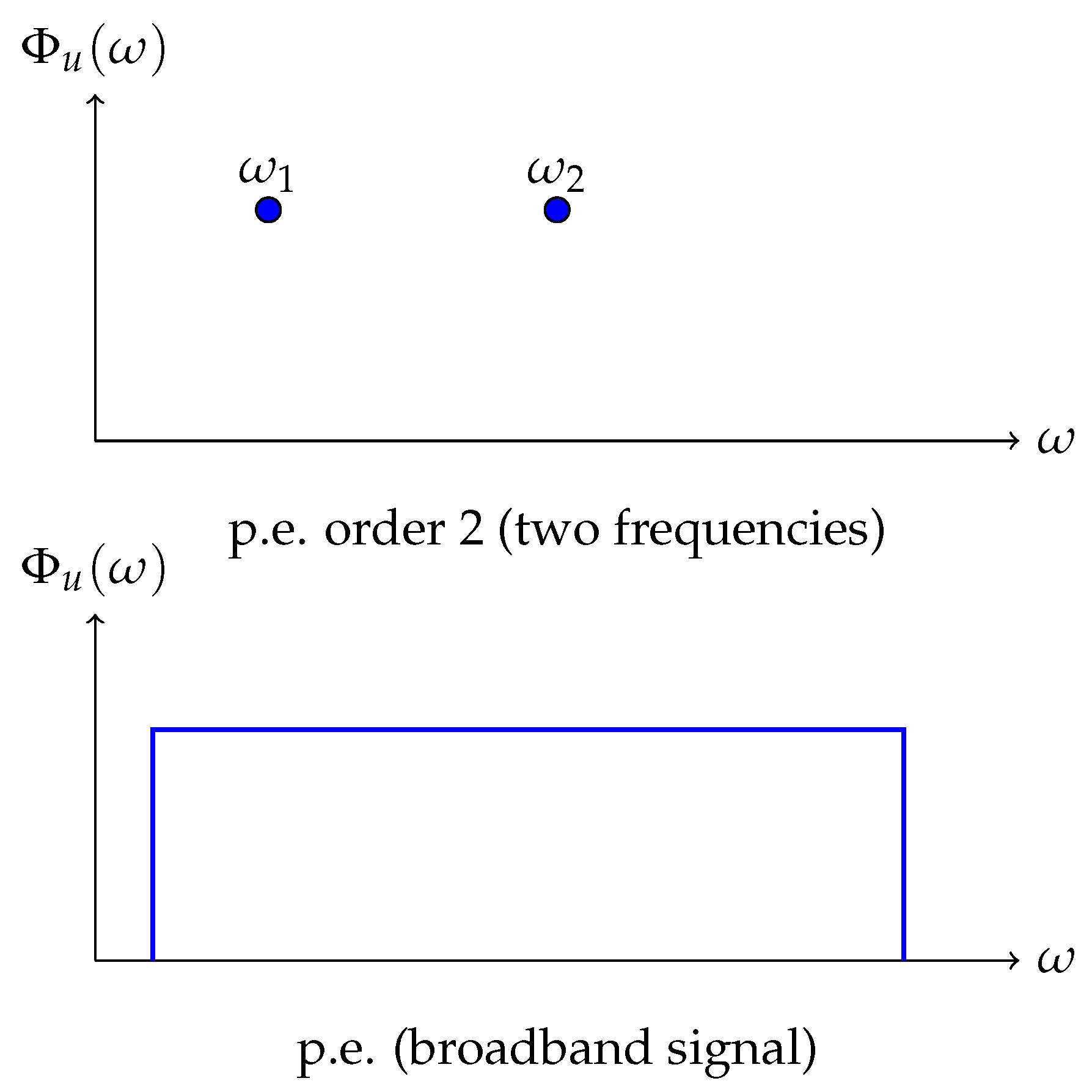
(Persistent Excitation of Order n, Ljung [1], Definition 13.1). A signal $\left\{u\right(t\left)\right\}$ with spectral density ${\Phi }_u\left(\omega \right)$ persistently excites order n (p.e. of order n) if for all non-trivial filters $M_n\left(q\right)={\sum }_{i=1}^n{m}_i{q}^{-i}$:

$$|M_n\left(e^{i\omega }\right){|}^2{\Phi }_u\left(\omega \right)\equiv 0\Rightarrow M_n\left(e^{i\omega }\right)\equiv 0$$

(6)

In simple words: Persistent excitation of order n means that the input signal $u\left(t\right)$ contains enough frequency components to identify a model with n parameters. If the input signal contains only one frequency (for example, $u\left(t\right)=sin\left({\omega }_{0}t\right)$), then only the system behavior at this frequency can be determined. To identify a second-order model, at least two different frequencies are needed.

Physical example: To determine the mass m and spring stiffness k in the system $m\ddot{x}+kx=F\left(t\right)$, it is insufficient to apply force at a single frequency $F\left(t\right)=Asin\left({\omega }_{0}t\right)$. At one frequency, only the combination of parameters (resonant frequency ${\omega }_r=\sqrt{k/m}$) can be measured, but not m and k separately. The system needs to be excited at two or more frequencies to uniquely determine both parameters.

Lemma 1 

(Ljung [1], Lemma 13.1). A signal $u\left(t\right)$ persistently excites order n if and only if the Toeplitz matrix (autocorrelation matrix)

$${\overline{R}}_n=\left[\begin{array}{cccc}{R}_u\left(0\right)& R_u\left(1\right)& \dots & R_u(n-1)\\ R_u\left(1\right)& R_u\left(0\right)& \dots & R_u(n-2)\\ ⋮& ⋮& \ddots & ⋮\\ R_u(n-1)& R_u(n-2)& \dots & R_u\left(0\right)\end{array}\right]$$

(7)

is non-singular, where $R_u\left(\tau \right)=\overline{E}\left[u\left(t\right)u(t-\tau )\right]$ is the autocorrelation function of the input signal.

In simple words: This is a specific mathematical criterion for persistent excitation. The matrix ${\overline{R}}_n$ is constructed from input signal autocorrelations. If it is non-singular (determinant $det\left({\overline{R}}_n\right)\ne 0$), then the signal is sufficiently rich for identifying a model of order n. If the matrix is singular, the signal is too “poor”—for example, it contains only one frequency or is constant.

2.4. Fisher Information Matrix: How Much Information About Parameters?

The central object in identification theory is the Fisher information matrix, which determines the amount of information about parameters contained in experimental data.

Definition 5 

(Fisher Information Matrix, Ljung [1], Section 9.2). For the prediction-error method, the Fisher information matrix is defined as

$$\overline{F}\left(\theta \right)=\overline{E}\left[\psi (t,\theta ){\psi }^T(t,\theta )\right]$$

(8)

where $\psi (t,\theta )=-{\displaystyle \frac{\partial \epsilon (t,\theta )}{\partial \theta }}$ is the gradient of the prediction error $\epsilon (t,\theta )=y\left(t\right)-\widehat{y}\left(t\right|\theta )$.

In simple words: The Fisher information matrix $\overline{F}\left(\theta \right)$ is a measure of how sensitive the observed data is to changes in parameters $\theta$. If a small change in parameter ${\theta }_i$ leads to a large change in the output signal $y\left(t\right)$, then the gradient $\partial y/\partial {\theta }_i$ is large, and the Fisher matrix contains much information about this parameter. The reverse is not true: if a parameter change almost does not affect observations, then the information about it is small.

The rank of the matrix $\overline{F}\left(\theta \right)$ determines local identifiability:

$$\mathrm{rank}\left(\overline{F}\left(\theta \right)\right)=d\iff \mathrm{local}\mathrm{identifiability}\mathrm{of}\mathrm{all}d\mathrm{parameters}$$

(9)

Physical meaning: If $\mathrm{rank}\left(\overline{F}\right)<d$, then some parameters are “hidden”—their change does not affect observable data, and they cannot be determined experimentally. For example, for the system $m\ddot{x}=F\left(t\right)$ with zero input $F\equiv 0$, the information about mass m is zero: $\mathrm{rank}\left(\overline{F}\right)=0$.

2.5. Hankel Matrix: Minimal Model Complexity

For linear systems, there is a close relationship between Fisher information and the Hankel matrix of the system.

Definition 6 

(Hankel Matrix). For a linear system with impulse response $g\left(k\right)$ ($k=1,2,3,\dots$), the Hankel matrix is constructed as

$$\mathcal{H}=\left[\begin{array}{cccc}g\left(1\right)& g\left(2\right)& g\left(3\right)& \dots \\ g\left(2\right)& g\left(3\right)& g\left(4\right)& \dots \\ g\left(3\right)& g\left(4\right)& g\left(5\right)& \dots \\ ⋮& ⋮& ⋮& \ddots \end{array}\right]$$

(10)

In simple words: The impulse response $g\left(k\right)$ is the system response to a unit impulse $\delta \left(t\right)$ (an instantaneous hit). The Hankel matrix is constructed from shifts of this response. The element ${\mathcal{H}}_{ij}=g(i+j-1)$ depends only on the sum of indices.

Theorem 1 

(Hankel Rank and System Order, Ljung [1], Section 4.3). The rank of the Hankel matrix $\mathcal{H}$ equals the order of the minimal realization of the system:

$$\mathrm{rank}\left(\mathcal{H}\right)=n\iff \mathrm{minimal}\mathrm{system}\mathrm{order}=n$$

(11)

In simple words: The system order is the minimal number of first-order differential equations (or states in a state-space model) necessary to describe the dynamics. The Hankel matrix rank gives this minimal order. For the system $m\ddot{x}=F$ with transfer function $G\left(s\right)=1/\left(m{s}^2\right)$, the impulse response $g\left(t\right)=t/m$ grows linearly, and $\mathrm{rank}\left(\mathcal{H}\right)=2$.

Physical example: Consider a free particle ($F=m\ddot{x}$). After a unit force impulse, the particle moves with constant velocity, the coordinate grows linearly: $x\left(t\right)=vt$. In discrete time $g\left(k\right)=k{T}_s/m$. The Hankel matrix:

$$\mathcal{H}={\displaystyle \frac{T_s}{m}}\left[\begin{array}{cccc}1& 2& 3& \dots \\ 2& 3& 4& \dots \\ 3& 4& 5& \dots \\ ⋮& ⋮& ⋮& \ddots \end{array}\right]$$

(12)

All rows are linearly dependent (each subsequent one is a shift of the previous), but any two rows are linearly independent. Therefore, $\mathrm{rank}\left(\mathcal{H}\right)=2$, which corresponds to a second-order system.

2.6. Asymptotic Accuracy of Parameter Estimates

Theorem 2 

(Ljung [1], Theorem 9.1). Under regularity conditions (ergodicity of signals, stability of the system), the parameter estimate ${\widehat{\theta }}_N$ obtained from N observations is asymptotically normal:

$$\sqrt{N}({\widehat{\theta }}_N-{\theta }_0)\stackrel{d}{\to }\mathcal{N}(0,P_{\theta })$$

(13)

where the covariance matrix

$$P_{\theta }={\lambda }_0{\left[\overline{F}\left({\theta }_0\right)\right]}^{-1}$$

(14)

${\lambda }_0$ is the prediction error variance, $\overline{F}$ is the Fisher information matrix from (8).

In simple words: This theorem states that with a large number of observations N, the parameter estimation error ${\widehat{\theta }}_N-{\theta }_0$ is normally distributed with variance proportional to $1/N$ and inversely proportional to the Fisher information matrix. The more information about parameters (larger $\overline{F}$), the more accurate the estimate.

Physical meaning: The variance of parameter estimate i:

$$\mathrm{Var}\left({\widehat{\theta }}_i\right)\propto {\displaystyle \frac{{\lambda }_0}{N}}·{\left[{\overline{F}}^{-1}\right]}_{ii}$$

(15)

If the element ${\left[\overline{F}\right]}_{ii}$ is small (parameter weakly affects output), then the variance is large—the parameter is determined inaccurately. If ${\left[\overline{F}\right]}_{ii}$ is large (strong influence), the variance is small—accurate estimate.

In the frequency domain (Ljung [1], Section 9.4, formula (9.37)):

$$P_{\theta }={\displaystyle \frac{{\lambda }_0}{2\pi }}{\left[{\int }_{-\pi }^{\pi }{\Psi }^{*}(e^{i\omega },{\theta }_0){\Phi }_u^{-1}\left(\omega \right)\Psi (e^{i\omega },{\theta }_0)d\omega \right]}^{-1}$$

(16)

where $\Psi (e^{i\omega },\theta )={\displaystyle \frac{\partial G(e^{i\omega },\theta )}{\partial \theta }}$ is the gradient of the transfer function with respect to frequency.

In simple words: This formula shows that estimation accuracy depends on the input signal spectrum ${\Phi }_u\left(\omega \right)$ and the sensitivity of the transfer function to parameters $\Psi (\omega ,\theta )$. If the input signal has high power at frequencies where the system is sensitive to parameters, then the estimate is accurate. If the input spectrum is concentrated at frequencies where the gradient $\Psi$ is small, accuracy decreases.

3. Newton’s First Law: Non-Informativeness Under Zero Excitation

3.1. Traditional Formulation

Newton’s first law states: in the absence of external forces (or when their vector sum equals zero) $\sum {\mathbf{F}}_i=0$, the acceleration of a body equals zero, i.e., $d\mathbf{v}/dt=0$. A consequence is the conservation of velocity: a body either remains at rest or moves uniformly and rectilinearly.

Traditional interpretation: This is an ontological statement about the nature of inertia—the property of matter to “resist changes in velocity.” The first law postulates the existence of inertial reference frames and defines the state of “natural motion” in the absence of influences.

3.2. Reinterpretation Through Data Informativeness

Consider the first law from the perspective of identification theory. If the external influence is absent ($u\left(t\right)\equiv 0$), what can be learned about the system dynamics from observations of the output $y\left(t\right)$?

Proposition 1 

(Non-Informativeness of Data with Zero Input). At $u\left(t\right)\equiv 0$, the data set $Z^{\infty }={\{u\left(t\right),y\left(t\right)\}}_{t=1}^{\infty }$ is non-informative with respect to the model structure (Definition 8.2 from Section 2).

Proof. 

At $u\left(t\right)\equiv 0$, the input spectral density ${\Phi }_u\left(\omega \right)\equiv 0$ for all frequencies $\omega$. According to Lemma 13.1 (Section 2.3), the Toeplitz matrix:

$${\overline{R}}_n=\left[\begin{array}{cccc}{R}_u\left(0\right)& R_u\left(1\right)& \dots & R_u(n-1)\\ R_u\left(1\right)& R_u\left(0\right)& \dots & R_u(n-2)\\ ⋮& ⋮& \ddots & ⋮\\ R_u(n-1)& R_u(n-2)& \dots & R_u\left(0\right)\end{array}\right]={\mathbf{0}}_{n\times n}$$

(17)

is singular for any $n\ge 1$, since all autocorrelations $R_u\left(\tau \right)=\overline{E}\left[u\left(t\right)u(t-\tau )\right]=0$ at $u\equiv 0$. Consequently, the signal $u\left(t\right)$ is not persistently exciting of any order n nor in the general sense of Definition 13.2.

Consider two distinct predictors (models) $W_1\left(q\right)$ and $W_2\left(q\right)$ of different orders. With zero input $u\equiv 0$, both models produce identical output signals determined only by initial conditions:

$$y\left(t\right)=v_{0}t+x_0$$

(18)

where $v_0$ is the initial velocity, $x_0$ is the initial coordinate. Different models are indistinguishable from the data, hence the data is non-informative. □

In simple words: If no external forces act on a system ($F\equiv 0$), then the body coordinate changes as $x\left(t\right)=v_{0}t+x_0$—a linear function of time. From such a trajectory, it is impossible to determine either the body mass or any other dynamic parameters. Any model—be it $m\ddot{x}=0$, or a more complex system with friction and springs with zero interaction forces—will produce the same linear trajectory. The data contains no information about the model structure.

Physical example: Imagine observing a body moving with constant velocity in a straight line in space. Can its mass be determined? No, because any body (light or heavy) in the absence of forces moves identically—uniformly and rectilinearly. To determine mass, it is necessary to apply a force and observe acceleration ($a=F/m$). Without force excitation, information about mass is fundamentally inaccessible.

Theorem 3 

(Information Indistinguishability of Models Under Zero Excitation). At $u\left(t\right)\equiv 0$, it is impossible to distinguish models of various orders $n\ge 1$ from experimental data ${\left\{y\left(t\right)\right\}}_{t=1}^{\infty }$.

Proof. 

According to Theorem 13.1 in [1], to identify the transfer function

$$G(q,\theta )={\displaystyle \frac{B(q,\theta )}{F(q,\theta )}}$$

(19)

with $n_b+n_f$ parameters, persistent excitation of order at least $n_b+n_f$ is necessary. At $u\left(t\right)\equiv 0$, this condition is not satisfied for any $n\ge 1$, since, as shown above, the matrix ${\overline{R}}_n$ is singular.

Moreover, the Fisher information matrix (8) at $u\equiv 0$ becomes zero:

$$\overline{F}\left(\theta \right)=\overline{E}\left[\psi (t,\theta ){\psi }^T(t,\theta )\right]=\mathbf{0}$$

(20)

where $\psi (t,\theta )=-{\displaystyle \frac{\partial \epsilon (t,\theta )}{\partial \theta }}$. This occurs because at zero input, the output does not depend on the transfer function parameters $\theta$ (it depends only on initial conditions), hence the gradient $\psi =0$.

Since $\mathrm{rank}\left(\overline{F}\right)=0$, parameter identification $\theta$ is impossible according to the theorem on the relationship between information matrix rank and identifiability (Section 2.4). □

In simple words: The Fisher information matrix $\overline{F}\left(\theta \right)$ measures the sensitivity of observed data to model parameters. At zero input $F\equiv 0$, the output signal (body trajectory) does not depend on system parameters at all—it is determined only by initial conditions $x\left(0\right)$ and $v\left(0\right)$. Changing the mass m, adding a spring with stiffness k, or friction with coefficient c will not affect uniform rectilinear motion in any way. Consequently, the gradient of output with respect to parameters equals zero, and the information matrix is singular.

Analogy: Attempting to determine car characteristics (engine power, mass, aerodynamic drag) while observing it rolling coasting on a level road with the engine and brakes off. All cars roll identically—at constant velocity (if friction is neglected). To distinguish a light sports car from a heavy truck, it is necessary to press the gas or brakes—that is, apply excitation.

3.3. Reformulation of the First Law in Terms of Identifiability

Hypothesis 1 

(Newton’s First Law as an Identifiability Boundary). In the absence of persistent excitation ($u\left(t\right)\equiv 0$), experimental data is non-informative with respect to the dynamic model structure of order $n\ge 1$. The only experimentally verifiable statement is the constancy of velocity $\mathbf{v}=\mathrm{const}$ (a zero-order model in terms of identification theory). The Fisher information matrix is singular: $\mathrm{rank}\left(\overline{F}\right)=0$.

In simple words: Newton’s first law is not a statement that “velocity is preserved,” but a statement about the boundary of the knowable: without external influence, no information about system dynamic properties can be obtained. Everything that can be experimentally verified at $F=0$ is that velocity is constant. Any hypotheses about body mass, internal forces, or model structure remain unverifiable.

Epistemological shift: The traditional formulation “a body preserves velocity in the absence of forces” sounds like an ontological statement about the nature of matter. The proposed reformulation “in the absence of excitation, data is non-informative with respect to dynamics” is an epistemological statement about the boundaries of information extraction from experiment. This does not deny the predictive power of the first law, but clarifies its methodological status.

Practical consequence: To experimentally determine any dynamic characteristics of a system (mass, moment of inertia, elasticity coefficients, etc.), it is necessary to ensure persistent excitation of sufficient order. Passive observation of free motion provides no information about parameters.

Connection to philosophy of science: This reformulation resonates with Bridgman’s operationalism—physical concepts are defined through their measurement procedures. Mass, force, inertia are not “entities” existing independently of the identification procedure. The first law defines the boundary beyond which the identification procedure becomes impossible.

4. Newton’s Second Law: Mass as a Conditioning Parameter

4.1. Traditional Formulation

Newton’s second law: $\mathbf{F}=m\mathbf{a}$, or in expanded form $\mathbf{F}=m{\displaystyle \frac{d^2\mathbf{x}}{d{t}^2}}$.

Traditional interpretation: This is a causal statement—force “causes” acceleration, and mass “resists” acceleration. Mass is understood as a measure of inertia—a fundamental property of matter.

4.2. Transfer Function and Hankel Rank

Consider the second law as an operator relationship between input (force F) and output (coordinate x). In continuous time with zero initial conditions, the Laplace transform gives:

$$F\left(s\right)=m{s}^{2}X\left(s\right)\Rightarrow G\left(s\right)={\displaystyle \frac{X\left(s\right)}{F\left(s\right)}}={\displaystyle \frac{1}{m{s}^2}}$$

(21)

In simple words: The transfer function $G\left(s\right)$ shows how the system transforms the input signal (force) into the output (coordinate) in the frequency domain. The operator s corresponds to differentiation: $s\leftrightarrow d/dt$, $s^2\leftrightarrow d^2/d{t}^2$. The relationship $X\left(s\right)={\displaystyle \frac{1}{m{s}^2}}F\left(s\right)$ means that to obtain the coordinate, the force (divided by mass) must be integrated twice: first, velocity is obtained $v=\int F/mdt$, then coordinate $x=\int vdt$.

The impulse response is the system response to a unit force impulse (an instantaneous hit) $F\left(t\right)=\delta \left(t\right)$:

$$g\left(t\right)={\mathcal{L}}^{-1}\left\{{\displaystyle \frac{1}{m{s}^2}}\right\}={\displaystyle \frac{t}{m}}$$

(22)

Physical meaning: If a body is struck by a unit impulse (momentum $p_0=1$ is transferred in an infinitely short time), it acquires velocity $v=p_0/m=1/m$ and then moves uniformly: $x\left(t\right)=vt=t/m$. The impulse response grows linearly with time.

The Hankel matrix (10) for the discretized signal $g\left(k\right)=k{T}_s/m$ ($k=1,2,3,\dots$):

$$\mathcal{H}={\displaystyle \frac{T_s}{m}}\left[\begin{array}{ccccc}1& 2& 3& 4& \dots \\ 2& 3& 4& 5& \dots \\ 3& 4& 5& 6& \dots \\ 4& 5& 6& 7& \dots \\ ⋮& ⋮& ⋮& ⋮& \ddots \end{array}\right]$$

(23)

Each row is a shift of the previous one by one position. It is easy to verify that $\mathrm{rank}\left(\mathcal{H}\right)=2$: any two rows are linearly independent (for example, the first and second: $(1,2,3,\dots )$ and $(2,3,4,\dots )$ are not proportional), but the third row is expressed through the first two: row 3 = 2·row 2 - row 1.

In simple words: Hankel rank shows the “true dimension” of system dynamics. For a free particle ($F=m\ddot{x}$), rank = 2 means that the system is completely described by two numbers: coordinate x and velocity v. This is the minimal state-space representation. It is impossible to describe dynamics with one number (that would be a static system), but two are sufficient.

Proposition 2 

(Minimality of Second Order). The transfer function $G\left(s\right)=1/\left(m{s}^2\right)$ has the minimal order among non-trivial identifiable models of a mechanical system.

Proof. 

Consider the hierarchy of transfer functions $G_n\left(s\right)=1/s^n$ with various orders n:

• $n=0$: $G_0\left(s\right)=1$—static system without dynamics. Input is instantaneously transmitted to output: $y\left(t\right)=u\left(t\right)$. This corresponds to the first law ($\dot{v}=0$ at $F=0$)—no memory, no inertia.
• $n=1$: $G_1\left(s\right)=1/s$—simple integrator. Impulse response $g\left(t\right)=\mathrm{const}$ (step). The Hankel matrix has $\mathrm{rank}\left(\mathcal{H}\right)=1$. Physically, this corresponds to a system where force directly determines velocity: $v=F/c$ (motion in a viscous medium at low Reynolds numbers). Insufficient for describing inertial dynamics—no second derivative.
• $n=2$: $G_2\left(s\right)=1/s^2$—double integrator. Impulse response $g\left(t\right)=t$ grows linearly. Hankel rank $\mathrm{rank}\left(\mathcal{H}\right)=2$. This is the minimal non-trivial identifiable model describing inertial motion.
• $n>2$: Transfer functions $1/s^3$, $1/s^4$, etc., have impulse responses $g\left(t\right)=t^2/2$, $g\left(t\right)=t^3/6$, and so on. Hankel rank increases: rank = 3, 4, ... However, such models are physically unrealistic for a point mass and excessively complex. At typical noise levels (SNR), adding poles above second order does not improve identifiability—additional parameters “sink” in noise.

According to Theorem 13.1 in [1], to identify a model with $n_b+n_f$ parameters, persistent excitation of order at least $n_b+n_f$ is necessary. For the transfer function $G\left(s\right)=1/\left(m{s}^2\right)$, there is one parameter (m), and for its identification, p.e. order 2 is sufficient, i.e., excitation at two different frequencies.

Thus, $n=2$ is the minimal order that:

1.

Describes non-trivial dynamics (differs from static and simple integrator)

2.

Physically corresponds to inertial motion

3.

Is identifiable under reasonable experimental conditions (two excitation frequencies)

□

In simple words: The second law $F=m\ddot{x}$ defines the minimal dynamic model that: - Is non-trivial (does not reduce to instantaneous transmission $y=u$) - Is experimentally identifiable (with excitation at ≥ 2 frequencies) - Is sufficiently simple (contains no redundant parameters)

Order 0 model—this is the first law (no dynamics). Order 1 model—motion without inertia. Order 2 model—minimal inertial model. Higher orders are physically unjustified for a point mass.

Analogy: The choice of second-order model $G\left(s\right)=1/\left(m{s}^2\right)$ is like Occam’s razor in identification theory—the simplest model adequately describing observations. Order 0 model is too simple (does not describe inertia), third-order and higher models are excessively complex (add parameters that do not improve predictive power at typical noise levels).

4.3. Mass and Fisher Information Matrix

Consider how well mass m can be determined from experimental data ${\{F\left(t\right),x\left(t\right)\}}_{t=1}^N$. For the transfer function $G\left(s\right)=1/\left(m{s}^2\right)$, the gradient with respect to mass:

$${\displaystyle \frac{\partial G(s,m)}{\partial m}}=-{\displaystyle \frac{1}{m^2{s}^2}}$$

(24)

In simple words: This gradient shows how much the output signal $X\left(s\right)$ will change with a small change in mass m. The minus sign means that increasing mass decreases the response (a heavier body accelerates more slowly). The $1/m^2$ dependence shows that sensitivity decreases quadratically with mass increase—heavy bodies are more difficult to “probe” experimentally.

The Fisher information matrix in the frequency domain (formula (16) from Section 2.5):

$$\overline{F}\left(m\right)\propto {\int }_{-\pi }^{\pi }{\left|{\displaystyle \frac{\partial G\left(e^{i\omega }\right)}{\partial m}}\right|}^2{\Phi }_u\left(\omega \right)d\omega ={\int }_{-\pi }^{\pi }{\displaystyle \frac{{\Phi }_u\left(\omega \right)}{m^4{\omega }^4}}d\omega$$

(25)

where ${\Phi }_u\left(\omega \right)$ is the spectral density of the input signal (force).

In simple words: Fisher information sums (integrates) contributions from all frequencies in the input signal spectrum. The contribution of frequency $\omega$ is proportional to: - Signal power at this frequency: ${\Phi }_u\left(\omega \right)$ - System sensitivity: ${|\partial G/\partial m|}^2$

The denominator ${\omega }^4$ shows that low frequencies carry more information about mass than high ones. Physically: at low frequencies (slow force changes), inertia manifests more strongly.

The asymptotic variance of mass estimate from Theorem 9.1 (formula (14)):

$$\mathrm{Var}\left(\widehat{m}\right)={\displaystyle \frac{{\lambda }_0}{\overline{F}\left(m\right)}}\propto {\displaystyle \frac{m^4{\lambda }_0}{{\int }_{-\pi }^{\pi }{\Phi }_u\left(\omega \right)/{\omega }^{4}d\omega }}$$

(26)

where ${\lambda }_0$ is the measurement noise variance.

Why exactly second order? First-order model $\dot{x}=F/m$ would mean that an instantaneous force change instantaneously changes velocity, violating strict causality: future input ($F(t+\Delta t)$) would instantaneously influence current output ($v\left(t\right)$). Second order $\ddot{x}=F/m$ is the minimal structure with two states (position x and velocity $v=\dot{x}$), where input influences output through two integrating stages: $F\to \ddot{x}\to \dot{x}\to x$. This ensures $g\left(0\right)=0$ (strict causality from Section 1) and Hankel rank 2 (minimal non-trivial memory). In the transfer function $G\left(s\right)=1/\left(m{s}^2\right)$, two poles at zero correspond to two integrators—two degrees of freedom of identifiable state. Higher-order systems (jerk and above) are possible but unnecessary for describing basic mechanics by Occam’s principle.

In simple words: Mass determination accuracy: - Degrades proportionally to $m^4$—heavy objects are much harder to determine! - Degrades with noise growth ${\lambda }_0$—obvious - Improves if the input signal contains more low-frequency components (larger denominator)

The dependence $\mathrm{Var}\left(\widehat{m}\right)\propto m^4$ is critical: doubling mass increases variance by 16 times!

Physical example: Compare mass determination of a billiard ball ($m_1=0.2$ kg) and a spacecraft ($m_2={10}^5$ kg). If force is applied with the same spectrum and measured with the same noise, then the variance of spacecraft mass estimate:

$${\displaystyle \frac{\mathrm{Var}\left({\widehat{m}}_2\right)}{\mathrm{Var}\left({\widehat{m}}_1\right)}}={\left({\displaystyle \frac{m_2}{m_1}}\right)}^4={\left({\displaystyle \frac{{10}^5}{0.2}}\right)}^4\approx 6\times {10}^{22}$$

(27)

Accuracy drops catastrophically! Practically this means that to determine spacecraft mass with the same relative accuracy as a billiard ball, it is necessary to either massively increase input signal power (apply much greater forces), or reduce measurement noise by many orders of magnitude.

Proposition 3 

(Mass as a Conditioning Parameter). The condition number of the mass identification problem:

$$\kappa \left(m\right)={\displaystyle \frac{\mathrm{Var}\left(\widehat{m}\right)}{\mathrm{Var}\left(\widehat{m}\right){|}_{m=m_{\mathrm{ref}}}}}\propto {\left({\displaystyle \frac{m}{m_{\mathrm{ref}}}}\right)}^4$$

(28)

grows as the fourth power of mass, which indicates poor conditioning at large m.

In simple words: Conditioning characterizes the “sensitivity” of the problem to errors. A poorly conditioned problem is one where small measurement errors lead to large errors in parameter estimates. The dependence $\kappa \propto m^4$ means that the problem of mass determination becomes exponentially poorly conditioned with mass increase.

Practical consequence: For accurate mass determination of heavy objects, it is necessary:

1.

Use low-frequency excitation (increase $\int {\Phi }_u\left(\omega \right)/{\omega }^4$)

2.

Minimize measurement noise ${\lambda }_0$

3.

Increase experiment duration N (variance decreases as $1/N$ according to Theorem 9.1)

Philosophical context: The second law defines not the “nature of mass,” but the structure of a minimal model adequate for identifying inertial dynamics. This is an operationalist definition: mass is that which is identified through the relationship $F=m\ddot{x}$ under conditions of persistent excitation.

5. Third Law of Newton: Self-Consistency in Closed Systems

5.1. Traditional Formulation

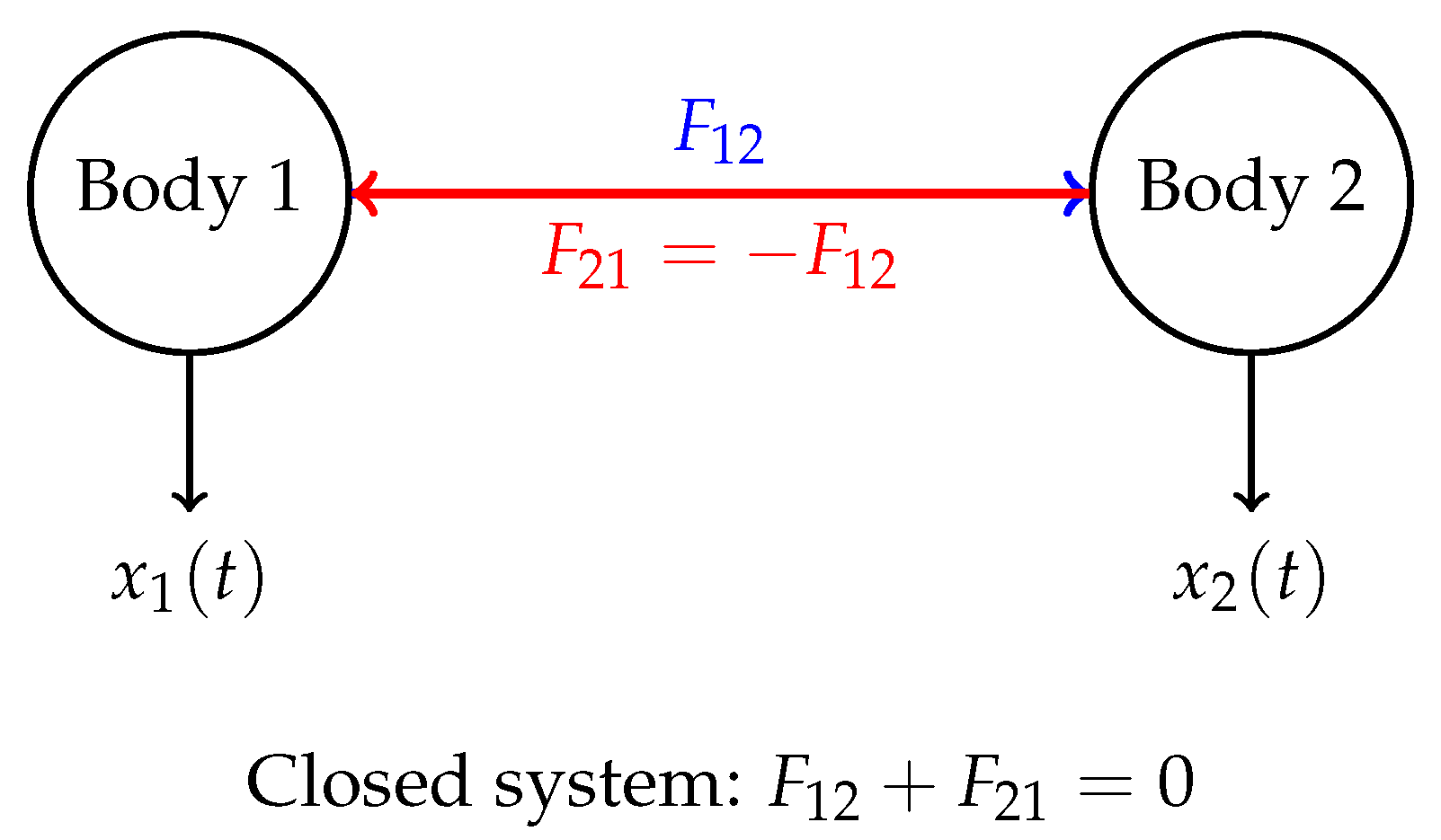
Newton’s Third Law: for any two interacting bodies, the forces of action and reaction are equal in magnitude and opposite in direction:

$${\mathbf{F}}_{12}=-{\mathbf{F}}_{21}$$

(29)

where ${\mathbf{F}}_{12}$ is the force acting from body 1 on body 2, and ${\mathbf{F}}_{21}$ is the force acting from body 2 on body 1.

Traditional interpretation: This is an ontological statement about the symmetry of interactions: “the action of one body on another always elicits an equal and opposite reaction.” The Third Law is considered a fundamental principle following from the homogeneity of space and time (through Noether’s theorem it is related to the conservation of momentum).

5.2. Identification in Closed Loops: The Indistinguishability Problem

Consider an attempt at independent identification of two interacting bodies. Write the equations of motion:

$$\begin{array}{cc}\hfill \mathrm{System}1:& m_1{\ddot{x}}_1=F_{21}\left(t\right)\Rightarrow \mathrm{model}{\mathcal{M}}_1\left({\theta }_1\right)\hfill \end{array}$$

(30)

$$\begin{array}{cc}\hfill \mathrm{System}2:& m_2{\ddot{x}}_2=F_{12}\left(t\right)\Rightarrow \mathrm{model}{\mathcal{M}}_2\left({\theta }_2\right)\hfill \end{array}$$

(31)

where ${\theta }_1=m_1$ and ${\theta }_2=m_2$ are the parameters to be identified.

In simple terms: Imagine observing two bodies interacting with each other (for example, two planets attracting gravitationally, or two magnets). Is it possible, based on observations of the trajectories $x_1\left(t\right)$ and $x_2\left(t\right)$, to determine the masses $m_1$ and $m_2$?

The problem is that the system is closed (closed-loop): the output of the first subsystem ($x_1$) affects the input of the second subsystem (the force $F_{12}$ depends on $x_1$), and vice versa. This creates a fundamental identifiability problem.

Physical example: Two planets orbiting a common center of mass. The gravitational force $F_{12}\propto m_1{m}_2/r^2$ depends on the distance $r=|x_2-x_1|$, which itself is determined by the motion of the planets. If only the trajectories $x_1\left(t\right)$ and $x_2\left(t\right)$ are observed, is it possible to uniquely determine both masses $m_1$ and $m_2$? It turns out that without additional conditions—no!

Ljung in [1], Section 13.4, provides a detailed analysis of identification in closed loops (closed-loop identification) and shows that it requires special conditions.

Theorem 4 

(Informativity in Closed Loop, Ljung [1], Theorem 13.2). A closed-loop experiment is informative if and only if the external excitation signal $r\left(t\right)$ (reference signal) is persistently exciting of sufficient order.

In simple terms: In a closed system (where the output of one subsystem affects the input of another), identification is possible only in the presence of an external excitation signal $r\left(t\right)$ that can be influenced independently. If the system is completely isolated ($r\equiv 0$), then uncertainty arises—different combinations of parameters can yield the same observed trajectories.

Diagram of a closed system with external excitation:

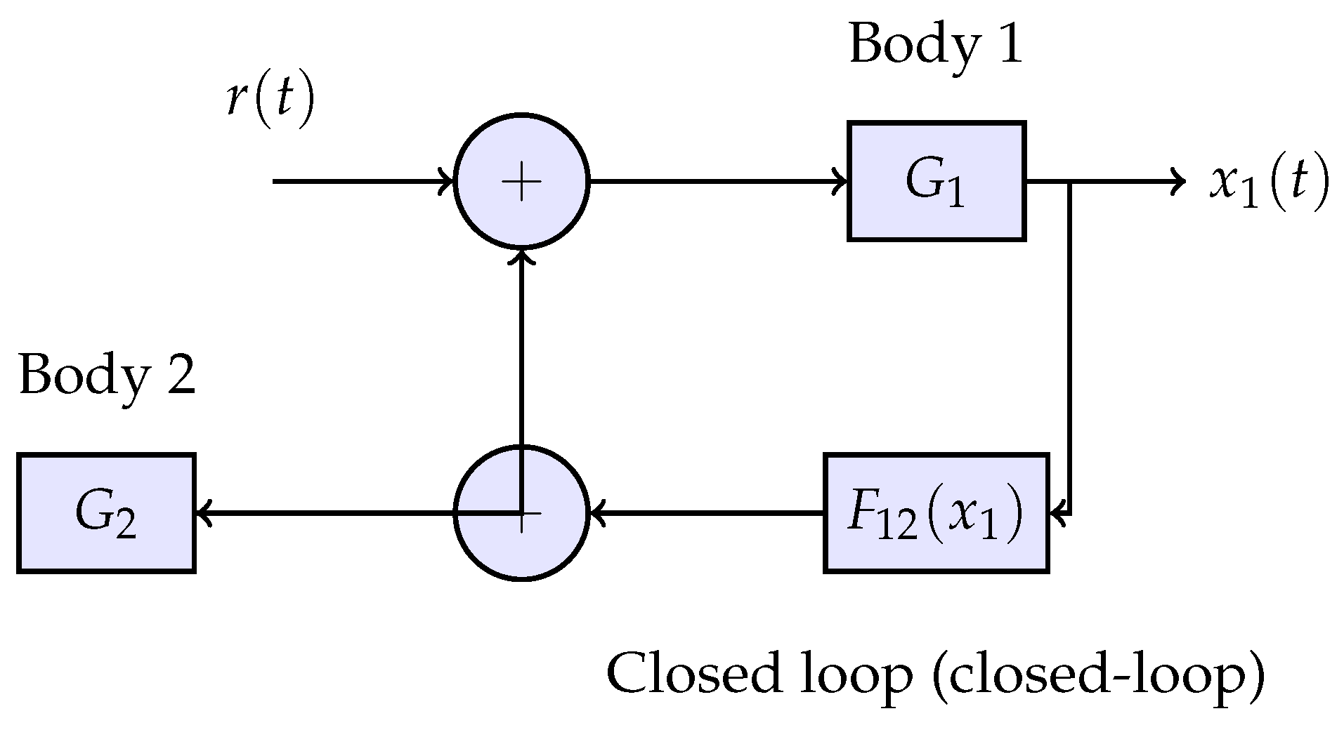
For an isolated system ($r\left(t\right)\equiv 0$, no external excitations), data informativity requires the condition:

$$F_{12}\left(t\right)+F_{21}\left(t\right)=0\forall t$$

(32)

In simple terms: If the system is completely isolated (no external influence $r\equiv 0$), then for the parameters of both subsystems to be uniquely identifiable, the interaction forces must satisfy the condition $F_{12}=-F_{21}$. Without this condition, uncertainty arises: infinitely many combinations $(m_1,m_2,F_{12},F_{21})$ yield the same trajectories.

Why does uncertainty arise? Consider a simplified example. Suppose two bodies are observed with trajectories $x_1\left(t\right)$ and $x_2\left(t\right)$. The equations are:

$$\begin{array}{cc}\hfill m_1{\ddot{x}}_1& =F_{21}\hfill \end{array}$$

(33)

$$\begin{array}{cc}\hfill m_2{\ddot{x}}_2& =F_{12}\hfill \end{array}$$

(34)

If $F_{12}$ and $F_{21}$ are independent functions, then there are 4 unknowns ($m_1,m_2,F_{12},F_{21}$) but only 2 observables ($x_1,x_2$). The system is underdetermined! However, if it is known that $F_{12}=-F_{21}$, then only 3 unknowns remain ($m_1,m_2,F_{12}$), and under certain conditions identification becomes possible.

Physical example—binary star: Two stars orbiting a common center of mass are observed. Only the trajectories on the celestial sphere are visible. Can both masses be determined? If Newtonian gravity $F=G{m}_1{m}_2/r^2$ and the Third Law $F_{12}=-F_{21}$ are assumed, then yes—the mass ratio can be determined from orbital kinematics. But if the Third Law were not satisfied (star 1 attracts star 2 with force $F_{12}$, but star 2 attracts star 1 with a different force $F_{21}\ne -F_{12}$), then the problem would become indeterminate.

5.3. Self-Consistency and Conjugacy of Operators

Hypothesis 2 

(Third Law as a Condition for Self-Consistency of Identification). For consistent identification of interacting subsystems in a closed system, the conjugacy of interaction operators is necessary: ${\widehat{F}}_{12}^{†}=-{\widehat{F}}_{21}$. This condition is equivalent to three requirements:

1.

Uniqueness of interaction channel: there exists one bidirectional channel, not two independent unidirectional ones

2.

Energy closure: energy is not created or destroyed in the interaction channel

3.

Identifiability of the combined structure: the joint model of the system has a finite Hankel rank

In simple terms: The Third Law $F_{12}=-F_{21}$ is not simply a “symmetry of forces” but a necessary condition for an isolated system of two interacting bodies to be identifiable. Without this condition: - Uncertainty arises in parameter identification - The system can spontaneously generate or lose energy (violation of energy closure) - The Hankel rank of the combined model becomes infinite (system is unidentifiable)

The three equivalent requirements are analyzed in detail below.

5.3.1. Uniqueness of Interaction Channel

If $F_{12}$ and $F_{21}$ are independent functions, this means there are two independent interaction channels: body 1 → body 2 (channel $F_{12}$) and body 2 → body 1 (channel $F_{21}$). The condition $F_{12}=-F_{21}$ reduces two channels to one bidirectional channel.

In simple terms: Imagine a channel as a “wire” connecting two bodies. If $F_{12}\ne -F_{21}$, then two independent wires are needed (one transmits force left to right, the other right to left). The Third Law states that one wire is sufficient, which pulls/pushes both bodies with equal force in opposite directions.

Consequence for identification: With one channel, fewer parameters need to be identified. If there are two channels, there are twice as many parameters, and the task is underdetermined.

5.3.2. Energy Closure

The power transmitted through the interaction channel:

$$P=F_{12}·{\dot{x}}_2+F_{21}·{\dot{x}}_1$$

(35)

If $F_{12}=-F_{21}=F$ and ${\dot{x}}_{rel}={\dot{x}}_2-{\dot{x}}_1$ is the relative velocity, then:

$$P=F({\dot{x}}_2-{\dot{x}}_1)=F·{\dot{x}}_{rel}$$

(36)

Energy is transmitted from body 1 to body 2 (or vice versa) without loss and without generation. However, if $F_{12}\ne -F_{21}$, then:

$$P=F_{12}·{\dot{x}}_2+F_{21}·{\dot{x}}_1\ne 0(\mathrm{in}\mathrm{general})$$

(37)

The system can spontaneously generate or lose energy in the interaction channel.

In simple terms: If the Third Law is not satisfied, the interaction channel can “create energy from nothing” or “absorb energy into nowhere.” Imagine a spring between two bodies: if the force acting on body 1 is not equal to the force acting on body 2 with opposite sign, then the spring itself becomes a source or sink of energy. This is physically absurd for a closed system.

Connection to identifiability: A system that spontaneously generates energy is self-excited. Its Hankel rank tends to infinity (the impulse response grows exponentially), and identification becomes impossible. This was shown in Section 8 (energy as an invariant norm): for identifiability of a closed system, energy conservation is necessary, which requires a norm-preserving evolution operator, which in turn requires $F_{12}=-F_{21}$.

5.3.3. Identifiability of the Combined Structure

For the combined system of two interacting bodies, the state-space model has the form:

$$\left[\begin{array}{c}{\dot{x}}_1\\ {\dot{v}}_1\\ {\dot{x}}_2\\ {\dot{v}}_2\end{array}\right]=\left[\begin{array}{cccc}0& 1& 0& 0\\ 0& 0& f_{12}/m_1& 0\\ 0& 0& 0& 1\\ f_{21}/m_2& 0& 0& 0\end{array}\right]\left[\begin{array}{c}{x}_1\\ v_1\\ x_2\\ v_2\end{array}\right]$$

(38)

where $f_{12}$ and $f_{21}$ are the coefficients of the interaction force (for example, for a spring $f=-k$).

If $f_{12}$ and $f_{21}$ are independent parameters, then the matrix has 4+2 = 6 independent parameters ($m_1,m_2,f_{12},f_{21}$, plus the structure). The Hankel rank of such a system is determined by the eigenvalues of the matrix. When $f_{12}·f_{21}>0$ (same sign), instability is possible—eigenvalues with positive real part, the system self-excites, rank($\mathcal{H}$) → ∞.

The condition $f_{21}=-f_{12}$ (equivalent to $F_{21}=-F_{12}$ for linear forces) ensures the symmetry of the matrix and the reality of eigenvalues (oscillatory dynamics without amplitude growth). The Hankel rank remains finite, and the system is identifiable.

In simple terms: The Third Law guarantees that the combined system of two interacting bodies has finite complexity (finite Hankel rank) and can be identified from experimental data. Without the Third Law, the complexity of the model can become infinite (self-excitation, unbounded growth of trajectories), making identification impossible.

Physical example—harmonic oscillator: Two bodies connected by a spring. Force on body 1: $F_1=-k(x_1-x_2)$. Force on body 2: $F_2=-k(x_2-x_1)=+k(x_1-x_2)=-F_1$. The Third Law is automatically satisfied! The system has two normal modes (in-phase and anti-phase oscillations), Hankel rank = 4 (two modes × two states per mode). Everything is identifiable.

Now imagine a “pathological spring” that acts on body 1 with force $F_1=-k_1(x_1-x_2)$ and on body 2 with force $F_2=-k_2(x_2-x_1)$, where $k_1\ne k_2$. The Third Law is violated! If $k_1>0$ and $k_2<0$, then the spring “repels” from one end and “attracts” from the other—absurdity, the system self-excites. Hankel rank → ∞, identification is impossible.

5.4. Reframing the Third Law in Terms of Identifiability

Hypothesis 3 

(Newton’s Third Law as a Self-Consistency Condition). For consistent and informative identification of parameters of interacting subsystems in an isolated (closed) system, the condition of force conjugacy is necessary: ${\mathbf{F}}_{12}=-{\mathbf{F}}_{21}$. This condition is equivalent to the requirement of uniqueness of interaction channel, energy closure, and finiteness of the Hankel rank of the combined model.

In simple terms: The Third Law is not a statement about “equality of action and reaction” in an ontological sense, but a condition for the self-consistency of identification of an isolated system. Without the Third Law: - It is impossible to uniquely identify subsystem parameters (uncertainty) - Energy closure is violated (self-generation of energy) - The Hankel rank becomes infinite (system is unidentifiable)

Epistemological shift: Traditional formulation: “forces of action and reaction are equal”—an ontological statement about the nature of interactions. The proposed reframing: “conjugacy of interaction operators is necessary for identifiability of an isolated system”—a methodological statement about conditions for extracting information from data.

Practical consequence: When experimentally testing the Third Law (measuring $F_{12}$ and $F_{21}$), deviation from the condition $F_{12}+F_{21}=0$ may indicate: - Presence of hidden external influences (system is not isolated) - Energy dissipation in the interaction channel (for example, friction) - Measurement errors

The condition $F_{12}=-F_{21}$ itself is necessary for correct identification of system parameters.

Connection to philosophy of science: The Third Law in the proposed interpretation is a principle of model self-consistency. The requirement of operator conjugacy is analogous to the requirement of consistency of an axiomatic system in mathematics. If the Third Law were not satisfied, the model of classical mechanics would become internally contradictory (would allow self-excitation, energy violation), and parameter identification would become impossible.

Limitations: The Third Law in the form $F_{12}=-F_{21}$ is strictly satisfied only for instantaneous interactions. In relativistic theory, where interactions propagate at finite speed, the Third Law is violated locally (but is preserved integrally for the total momentum of field + particles). From the perspective of identifiability theory, this means that for relativistic systems, modification of identifiability conditions is necessary—the delay in the interaction channel must be taken into account.

6. Radical Ontological Differences Between the Two Interpretations

The proposed reinterpretation of Newton’s laws through system identification theory is not a simple translation of terms. It represents a fundamental shift in ontological and epistemological foundations. In this section, I explicitly enumerate which concepts from canonical mechanics are absent in the proposed framework, and what replaces them.

6.1. What is Absent in the Proposed Interpretation

6.1.1. Mass as an Intrinsic Objective Property of an Object

Canonical interpretation: Mass m is a fundamental property of a body, the “quantity of matter,” invariant in time and independent of measurement procedure. Mass exists objectively, independent of any observer.

Proposed interpretation: Mass m is a conditioning parameter of the identification problem, characterizing the accuracy with which this parameter can be determined from data:

$$\mathrm{Var}\left(\widehat{m}\right)\propto m^4$$

(39)

Mass is not an “intrinsic property of an object” existing independently of the identification procedure. Mass is what gets identified through the relation $F=m\ddot{x}$ when persistent excitation conditions are satisfied. Outside the identification procedure, the question “what is the mass of a body?” has no operational meaning.

In simple terms: In canonical mechanics, mass is like a “passport number” of an object—a permanent label inherent to the object. In the proposed framework, mass is like “degree of identification difficulty”—it characterizes not the object itself, but the complexity of the procedure for extracting information about it from data.

Consequence: The question “does mass change over time?” in canonical mechanics is an ontological question about conservation of matter. In the proposed framework, it is a question about stationarity of model parameters: can we use a time-invariant model, or do parameters $\theta \left(t\right)$ change?

6.1.2. Space and Coordinate Grid as a Geometric Entity

Canonical interpretation: There exists absolute space (in Newton) or pseudo-Euclidean spacetime (in relativistic mechanics)—a geometric arena on which physical processes unfold. Coordinates $(x,y,z)$ are labels of points in this space.

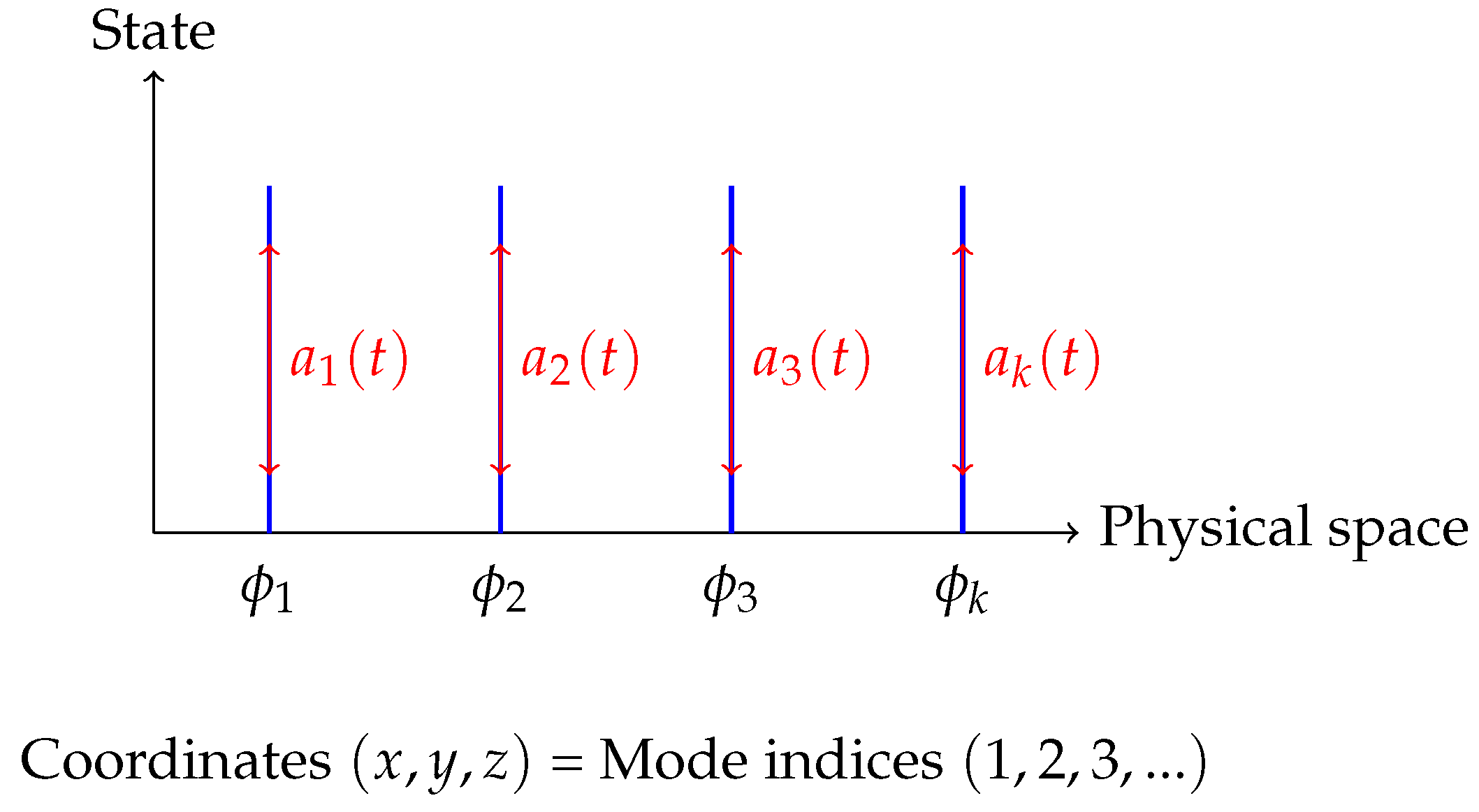
Proposed interpretation: Coordinates are indices of spectral modes in the state expansion (Section 6):

$$x\left(t\right)=\sum _{k=1}^{\infty }{a}_k\left(t\right){\varphi }_k$$

(40)

There is no assumption about the existence of “geometric space.” A coordinate $(x,y,z)$ is a triplet of indices $(1,2,3)$ numbering the eigenfunctions (modes) in some decomposition. Coordinate transformation is mode renumbering.

In simple terms: In canonical mechanics, coordinates are “addresses” in space, like latitude and longitude on a map. In the proposed framework, coordinates are “channel numbers” in spectral decomposition, like frequencies on a radio (FM 87.5, FM 88.0, FM 88.5...). There is no “space of radio waves,” there is a frequency spectrum.

Consequence: The question “is space homogeneous?” in canonical mechanics is a question about geometry. In the proposed framework, it is a question about whether the system is invariant to mode renumbering (symmetry with respect to cyclic permutations of indices).

6.1.3. Force as an Important Physical Entity

Canonical interpretation: Force $\mathbf{F}$ is a fundamental concept, the “cause of change in motion,” a vector quantity. Forces are classified by nature (gravity, electromagnetism, elasticity) and have ontological status.

Proposed interpretation: “Force” $u\left(t\right)$ is simply the input signal in an identification experiment. There are no claims about the “nature” of force. What matters is only that the system input can be influenced (ensuring persistent excitation) and the output signal $y\left(t\right)$ can be observed.

In simple terms: In canonical mechanics, force is like an “agent of action”—an entity that “pushes” a body. In the proposed framework, “force” is like a “control knob” on an instrument—we turn it (set $u\left(t\right)$) and watch what happens on the screen (observe $y\left(t\right)$). There is no metaphysics of “pushing.”

Consequence: The question “what is force really?” in canonical mechanics is an ontological question. In the proposed framework, it is a meaningless question. Force is operationally that which we supply to the system input to excite it.

6.1.4. Global Clockwork of Time

Canonical interpretation: There exists absolute time t (in Newton) or a time coordinate in spacetime (in SR/GR), flowing uniformly and identically for all processes. Time is an independent variable, an “axis” along which the system evolves.

Proposed interpretation: Time does not play a special role. Instead of the time domain $\left(t\right)$, the primary domains are the frequency domain$\left(\omega \right)$ and the phase domain (complex s-plane: $s=\sigma +i\omega$). The transfer function $G\left(s\right)$ describes the system in the frequency domain, where “time” appears as a shift parameter (shift operator q) or as a discretization index.

In simple terms: In canonical mechanics, time is like “ticking clocks”—a universal metronome for the entire Universe. In the proposed framework, “time” is like a “frame index” in video recording—a discrete label for ordering observations. The main information is contained not in the sequence of frames $y\left(1\right),y\left(2\right),y\left(3\right),\dots$, but in the spectrum ${\Phi }_y\left(\omega \right)$—the decomposition of the signal by frequencies.

Technical clarification: Discussion in terms of time-shift indices (shift operator q, “historicity” regime) is possible only when the system possesses memory—it preserves traces of previous states, i.e., temporal correlations exist: $R(t,t+\tau )\ne 0$. This is possible only if the observation channel update does not completely erase previous states. For memoryless systems ($y\left(t\right)=f\left(u\right(t\left)\right)$), temporal indexing is meaningless—only the instantaneous input-output dependence matters.

Consequence: The question “does time flow uniformly?” in canonical mechanics is a question about the structure of time. In the proposed framework, it is a question about stationarity of the autocorrelation function $R_y\left(\tau \right)$: does correlation depend only on the time difference $\tau =t_2-t_1$, or also on absolute time $t_1$?

6.1.5. Action at a Distance Without Mechanism Explanation

Canonical interpretation: Gravitational or electrostatic interaction is described by a force acting instantaneously at a distance: $F\propto 1/r^2$. The mechanism of interaction transmission is either not discussed (Newton: “hypotheses non fingo”), or introduced through the concept of field (in relativistic theory).

Proposed interpretation: There is no postulate of “action at a distance.” There is only an interaction channel between subsystems, described by a transfer function or impulse response. The question is not “how is force transmitted through space,” but what is the structure of the channel: its order (Hankel rank), delay (strict causality), frequency response.

In simple terms: In canonical mechanics, “action at a distance” is like telepathy—body 1 “feels” body 2 located far away, without intermediary. In the proposed framework, we speak only of a communication channel: there is input $u_1\left(t\right)$ at one end, output $y_2\left(t\right)$ at the other end, and a transfer function $G_{12}\left(s\right)$ describing the channel. The question about “mechanism” is not posed—the question about identifiability of channel parameters is posed.

Consequence: The question “how is gravity transmitted through empty space?” in canonical mechanics is a deep ontological question that led to field theory. In the proposed framework, this is not a question at all. There is a channel with a certain impulse response $g\left(t\right)$, and if $g\left(t\right)\ne \delta \left(t\right)$ (not instantaneous response), then the channel has delay. The nature of the delay (finite propagation speed, field inertia) is outside the scope of identification theory.

6.2. What Exists Instead of Canonical Concepts

6.2.1. Electromagnetic Spectrum as Observation Channel

Central idea: Instead of abstract “coordinate space,” the primary object is the electromagnetic spectrum—the observation and interaction channel available to us for physical systems.

In simple terms: We do not “live in space $(x,y,z)$,” we observe through the electromagnetic channel. Any measurement (position of a body, its velocity, temperature) ultimately reduces to registration of electromagnetic radiation of a certain frequency and phase. We can influence the system by sending electromagnetic signals (photons of certain frequencies) and observe the response—changes in the emission spectrum.

Khinchin’s spectral representation theorem: For a stationary random process $y\left(t\right)$, there exists a spectral decomposition:

$$y\left(t\right)={\int }_{-\infty }^{\infty }{e}^{i\omega t}dZ\left(\omega \right)$$

(41)

where $Z\left(\omega \right)$ is a process with orthogonal increments, and the autocorrelation function:

$$R_y\left(\tau \right)={\int }_{-\infty }^{\infty }{e}^{i\omega \tau }{\Phi }_y\left(\omega \right)d\omega$$

(42)

In simple terms: Khinchin’s theorem states that any stationary process can be decomposed by frequencies (like sound decomposes into tones in music). The spectral density ${\Phi }_y\left(\omega \right)$ completely characterizes the statistical properties of the signal. This is a fundamental result on which all frequency-domain identification theory is built.

Consequence: Instead of the question “what are the coordinates of a body in space?” we pose the question “what is the spectral density ${\Phi }_y\left(\omega \right)$ of radiation observed from the system?”

6.2.2. Frequency and Phase Domain Instead of Time Domain

The transfer function $G\left(s\right)$ in the complex s-plane ($s=\sigma +i\omega$) contains complete information about a linear system. Time evolution $y\left(t\right)$ is merely the inverse Laplace transform:

$$y\left(t\right)={\mathcal{L}}^{-1}\left\{G\left(s\right)U\left(s\right)\right\}={\displaystyle \frac{1}{2\pi i}}{\int }_{\gamma -i\infty }^{\gamma +i\infty }G\left(s\right)U\left(s\right)e^{st}ds$$

(43)

In simple terms: “Time” is a derived construction obtained from frequency decomposition. Primary is the frequency response $G\left(i\omega \right)$—how the system responds to sinusoidal excitation at different frequencies. Knowledge of $G\left(i\omega \right)$ for all $\omega$ completely determines system behavior.

Practical consequence: In an identification experiment, we do not “track coordinate $x\left(t\right)$ over time,” but measure the frequency response—amplitude and phase of the response at each frequency. From the frequency response we reconstruct the transfer function $G\left(s\right)$, from it—the model parameters $\theta$.

6.2.3. Fisher Information Matrix and Cramér-Rao Bound

Central concept: Instead of “force,” “mass,” “space,” the central object becomes the Fisher information matrix $\overline{F}\left(\theta \right)$, determining the boundaries of knowability.

The inverse Fisher matrix is the Cramér-Rao bound:

$$\mathrm{Cov}\left(\widehat{\theta }\right)\ge {\overline{F}}^{-1}\left(\theta \right)$$

(44)

In simple terms: For any unbiased parameter estimation method, the estimation variance cannot be less than the inverse Fisher matrix. This is a fundamental limitation on the accuracy with which we can extract information from data. The Cramér-Rao bound does not depend on the processing algorithm—it is determined only by the data itself and the model.

Physical meaning: Fisher information $\overline{F}\left(\theta \right)$ quantitatively characterizes “how much information about parameter $\theta$ is contained in experimental data.” If ${\overline{F}}_{ii}$ is small, then even an optimal method cannot accurately determine parameter ${\theta }_i$—the information is simply not there. If ${\overline{F}}_{ii}$ is large, then the parameter is accurately identifiable.

Consequence for Newton’s laws: - First law: $u\equiv 0\Rightarrow \overline{F}=0$ (zero information) - Second law: $\overline{F}\left(m\right)\propto m^{-4}$ (conditioning grows as $m^4$) - Third law: Condition $F_{12}=-F_{21}$ ensures finiteness of $\overline{F}$ for the combined system

6.2.4. Boundaries of Knowability BEFORE Model Construction

Radical methodological difference: In canonical mechanics, laws are first postulated ($F=ma$), then models are built, then tested experimentally. In the proposed approach, the order is reversed:

1.

First analyze identifiability boundaries: which models can in principle be distinguished from data?

2.

Then among identifiable models, choose the minimal in complexity (minimum Hankel rank)

3.

Finally verify whether experimental data are consistent with the chosen model

In simple terms: Instead of the question “what laws govern nature?” we pose the question “what models can we construct from available data at all?” This is an epistemological shift from ontology to methodology.

Practical consequence: Before building a grey-box model with specified structure ($F=m\ddot{x}$), we verify: - Is excitation sufficiently persistent? (rank(${\overline{R}}_n$) = n?) - Is Fisher information finite? (rank($\overline{F}$) = d?) - What is the Hankel rank of the data? (minimum model order?)

Only after this does it make sense to fit model parameters.

6.3. Conceptual Economy and Explanatory Power

Consider a thought experiment: two groups of students unfamiliar with classical mechanics are presented with two interpretations of Newton’s laws—canonical and proposed—for equal time, without historical baggage. Which interpretation is conceptually: - Cleaner (fewer undefined concepts)? - More economical (fewer basic postulates)? - More powerful (more practical consequences)?

6.3.1. Conceptual Cleanliness

Canonical interpretation requires accepting on faith:

• Existence of absolute space (or spacetime)
• Existence of mass as intrinsic property of body
• Existence of force as physical entity
• Action at a distance without mechanism
• Uniform flow of time

Proposed interpretation requires accepting:

• Existence of observation channel (electromagnetic spectrum)
• Ability to influence channel input and observe output
• Stationarity of processes (for applicability of Khinchin’s theorem)

In simple terms: Canonical interpretation introduces 5 metaphysical entities (space, time, mass, force, action-at-a-distance) that cannot be directly observed—only their consequences. Proposed interpretation introduces 1 observable entity (channel) and 2 operational assumptions (can influence, can observe). This is more economical in Occam’s razor sense.

6.3.2. Economy of Postulates

Canonical interpretation: - Three Newton’s laws (3 independent postulates) - Galilean relativity principle - Universal gravitation law (or other force laws) - Total: >= 4 independent postulates

Proposed interpretation: - Khinchin’s spectral representation theorem (mathematically proven) - Definition of identifiability (Definition 4.6, not a postulate but a definition) - Theorem on relation between Fisher rank and identifiability (mathematically proven) - Total: 0 physical postulates, everything follows from mathematical theorems

In simple terms: Canonical interpretation postulates laws of nature. Proposed interpretation derives boundaries of knowability from mathematical theorems of information theory and linear algebra. There are no physical postulates—only mathematical consequences of observation channel structure.

6.3.3. Practical Power

Canonical interpretation provides: - Equations of motion for solving mechanics problems - Qualitative understanding (inertia, action-reaction) - Foundation for grey-box modeling

Proposed interpretation provides: - All of the above, plus: - Quantitative identifiability criteria (rank($\overline{F}$), rank($\mathcal{H}$)) - Bounds on parameter estimation accuracy (Cramér-Rao bound) - Experiment design criteria (persistent excitation order n) - Understanding of when model is fundamentally unidentifiable

In simple terms: Canonical interpretation says “how nature works” (ontology). Proposed interpretation says “what we can know about nature and with what accuracy” (epistemology). The latter includes the former as a special case but adds quantitative criteria for boundaries of knowledge.

6.4. Practical Perspective: Model Usefulness

A key distinction of the proposed approach is emphasis on practical usefulness of models, not their “truth.”

Canonical logic: 1. Postulate laws (they are “true”) 2. Build models based on laws 3. Test experimentally 4. If doesn’t work—search for “new laws”

Proposed logic: 1. Run experiment, collect data $\left\{u\right(t),y(t\left)\right\}$ 2. Analyze identifiability boundaries (rank($\overline{F}$), rank($\mathcal{H}$)) 3. Build minimal model consistent with data 4. Evaluate model usefulness by criteria (prediction accuracy, parameter parsimony) 5. If usefulness insufficient—complexify model or improve experiment

In simple terms: Don’t ask “what is the nature of mass?” (metaphysics), ask “which model best predicts observations with minimum number of parameters?” (pragmatics).

Model usefulness criteria:

• Predictive power: how accurately does model predict $y\left(t\right)$ for new $u\left(t\right)$?
• Parameter parsimony: is Hankel rank minimal (Occam’s razor)?
• Identifiability: can parameters be reliably estimated (rank($\overline{F}$) = d)?
• Conditioning: how sensitive are estimates to noise (condition number)?

The question “is model $F=m\ddot{x}$ true?” is replaced by “is this model useful for this set of experiments?”

6.5. Historicity and Channel Memory

Technical clarification: Discussion in terms of time-shift indices (discrete time $t=1,2,3,\dots$, shift operator q) makes sense only for systems with memory.

A system has memory if output at time t depends not only on input at the same moment $u\left(t\right)$, but also on previous inputs $u(t-1),u(t-2),\dots$. Mathematically, this means presence of temporal correlations:

$$R_y\left(\tau \right)=\overline{E}\left[y\left(t\right)y(t-\tau )\right]\ne 0\mathrm{for}\tau >0$$

(45)

In simple terms: If system “remembers” the past (inertia, energy accumulation in spring, channel delay), then it makes sense to speak of “temporal evolution” and use time indexing. If system is memoryless ($y\left(t\right)=f\left(u\right(t\left)\right)$ depends only on current input), then temporal indexing is redundant—knowing instantaneous dependence $y=f\left(u\right)$ suffices.

Condition for memory presence: Observation channel must not completely “erase” previous states at each update. If system resets at each measurement, then correlations $R_y\left(\tau \right)=0$ for $\tau >0$, and temporal structure is absent.

Connection to Newton’s laws: Second-order model $F=m\ddot{x}$ has memory—current state $(x,v)$ is determined by entire history of applied forces. Hankel rank 2 means system “remembers” two recent states (coordinate and velocity). If system were memoryless (rank = 0), Newton’s laws would be trivial: $x=F$ (statics).

6.6. Section Conclusions

The proposed reinterpretation is not “just another language” for describing the same physical phenomena. It is a radically different ontology, where: - There are no absolute entities (mass, space, force, time) - There is only observation channel, its frequency response and identifiability boundaries - Questions “what exists?” are replaced by questions “what is identifiable?” - Truth criterion is replaced by model usefulness criterion

This does not deny the predictive power of classical mechanics. It clarifies its epistemological status: Newton’s laws are not revelations about “the nature of things,” but specifications of minimal identifiable models useful for describing a class of experiments.

If both interpretations are presented for equal time to students without historical baggage, the proposed interpretation will be: - Conceptually cleaner (fewer metaphysical entities) - More economical (0 physical postulates vs 3+ canonical) - More practical (quantitative criteria for knowledge boundaries)

Only one question remains: why does canonical interpretation dominate? Answer: historical inertia, entrenchment of geometric language, and the fact that for most engineering applications ontological questions don’t matter—only predictive power matters, which is identical for both interpretations.

7. Coordinates as Indices of Spectral Modes

7.1. Spectral Decomposition and Modes

The state of a linear system can be represented as a decomposition over eigenmodes:

$$x\left(t\right)=\sum _{k=1}^{\infty }{a}_k\left(t\right){\varphi }_k$$

(46)

where ${\varphi }_k$ are eigenfunctions (modes), $a_k\left(t\right)$ are amplitudes.

7.2. Coordinate Invariance and Minimal Realizations

In state-space representation (Ljung [1], Section 4.3), a system is specified by the triple $(A,B,C)$:

$$\begin{array}{cc}\hfill \dot{x}\left(t\right)& =Ax\left(t\right)+Bu\left(t\right)\hfill \end{array}$$

(47)

$$\begin{array}{cc}\hfill y\left(t\right)& =Cx\left(t\right)\hfill \end{array}$$

(48)

Similarity transformation $\tilde{x}=Tx$ yields an equivalent realization $(\tilde{A},\tilde{B},\tilde{C})$ with the same transfer function $G\left(s\right)$.

Proposition 4 

(Coordinate invariance of identifiability). Parameter identifiability does not depend on choice of coordinates if the transformation is invertible. The rank of the Hankel matrix is invariant to similarity transformations.

7.3. Center of Mass as Minimal Parameterization

For a system of N bodies, there exists a special coordinatization—the center of mass coordinate:

$$x_{cm}={\displaystyle \frac{{\sum }_{i=1}^N{m}_i{x}_i}{{\sum }_{i=1}^N{m}_i}}$$

(49)

Theorem 5 

(Center of mass and minimal Hankel rank). The center of mass coordinate is characterized by the property that in these coordinates internal interaction forces vanish (decoupling), and the system model has minimal Hankel rank.

For an isolated system ($\sum F_{\mathrm{ext}}=0$), the center of mass dynamics:

$$M_{\mathrm{total}}{\ddot{x}}_{cm}=0$$

(50)

corresponds to Hankel rank 1 (instead of $2N$ for the full system).

Proof. 

Summing the equations of motion for all bodies:

$$\sum _{i=1}^N{m}_i{\ddot{x}}_i=\sum _{i=1}^N{F}_i^{\mathrm{ext}}+\sum _{i<j}(F_{ij}+F_{ji})$$

(51)

Under the third law $F_{ij}+F_{ji}=0$, all internal forces cancel. For an isolated system ($\sum F_i^{\mathrm{ext}}=0$):

$${\ddot{x}}_{cm}=0\Rightarrow G_{cm}\left(s\right)={\displaystyle \frac{1}{s}}$$

(52)

The transfer function $1/s$ has Hankel rank 1, which is minimal for any parameterization of an isolated system. □

This shows that the center of mass is not simply a “convenient” coordinate, but “the unique parameterization with minimal model complexity” in the sense of identification theory.

8. Momentum as the Minimally Identifiable Conserved Quantity

8.1. Velocity as the First Stable Quantity

Coordinate $x\left(t\right)$ depends on the choice of reference point: $x\to x+x_0$. Velocity $v=dx/dt$ is invariant to shifts:

$$v\left(t\right)={\displaystyle \frac{dx}{dt}}\mathrm{does}\mathrm{not}\mathrm{depend}\mathrm{on}{x}_0$$

(53)

In terms of transfer functions for $G\left(s\right)=1/\left(m{s}^2\right)$:

$$X\left(s\right)={\displaystyle \frac{1}{m{s}^2}}F\left(s\right),V\left(s\right)=sX\left(s\right)={\displaystyle \frac{1}{ms}}F\left(s\right)$$

(54)

The transfer function from force to velocity $G_v\left(s\right)=1/\left(ms\right)$ has Hankel rank 1 and is the “minimally identifiable” quantity independent of initial conditions.

8.2. Momentum and the Coefficient at 1/s

Consider the spectral decomposition of the transfer function:

$$G\left(s\right)={\displaystyle \frac{c_0}{s^0}}+{\displaystyle \frac{c_1}{s^1}}+{\displaystyle \frac{c_2}{s^2}}+\dots$$

(55)

For a mechanical system $G\left(s\right)=1/\left(m{s}^2\right)$, the coefficient at $1/s$:

$$c_1=\underset{s\to 0}{lim}s·G\left(s\right)=\underset{s\to 0}{lim}{\displaystyle \frac{1}{ms}}=0$$

(56)

However, for the transfer function to velocity $G_v\left(s\right)=1/\left(ms\right)$:

$$c_1^{\left(v\right)}=\underset{s\to 0}{lim}s·G_v\left(s\right)={\displaystyle \frac{1}{m}}$$

(57)

Physically $c_1^{\left(v\right)}·F=v/m=p/\left(m^2\right)$ is related to momentum.

8.3. Momentum Conservation in Closed Channels

Theorem 6 

(Law of momentum conservation in identification terms). In a closed identifiable system (without external input $u\equiv 0$), the coefficient at $1/s$ in the spectral decomposition of the transfer function to velocity remains constant.

Proof. 

When $u\left(t\right)\equiv 0$, system dynamics are determined by initial conditions. For $G_v\left(s\right)=1/\left(ms\right)$, the response to initial condition $v_0$:

$$v\left(t\right)=v_0\left(\mathrm{constant}\mathrm{velocity}\right)$$

(58)

In the spectral domain:

$$V\left(s\right)={\displaystyle \frac{v_0}{s}}$$

(59)

The coefficient $c_1=v_0$ is preserved as $t\to \infty$, since any change would require external excitation.

More rigorously: The Hankel matrix for $G_v\left(s\right)=1/\left(ms\right)$ has rank 1. Changing $c_1$ without external input would increase the rank, contradicting the minimal realization principle for an isolated system. □

Physically, momentum $p=mv$ corresponds to $c_1·m=v_0·m$, and its conservation is a consequence of the absence of external excitation channel.

8.4. Non-Compensable 1/s² Mode and Identification Stability

A pole at $s=0$ of multiplicity 2 makes the system “marginally stable”. In identification theory (Ljung [1], Section 8.2), stability is usually required for guaranteed convergence of estimates.

However, for mechanical systems $G\left(s\right)=1/\left(m{s}^2\right)$, identification is possible due to:

1.

“Detectability”: output responds to input, although system does not decay

2.

“Bounded inputs”: physical forces are bounded

3.

“Finite Hankel rank”: rank($\mathcal{H}$) = 2 is finite

Practically, identification is performed with transformed data (e.g., difference encoding) or in closed-loop with a controller ensuring stability.

8.5. Center of Mass and Uniqueness of Parameterization

Returning to the many-body system: in center of mass coordinates, internal interaction forces are decoupled, and what remains is:

$$G_{cm}\left(s\right)={\displaystyle \frac{1}{M_{\mathrm{total}}s}}$$

(60)

This is the unique parameterization where:

• Hankel rank is minimal (rank = 1)
• Coefficient at $1/s$ corresponds to total system momentum
• There are no internal couplings (minimal model)

Remark 1. 

In traditional mechanics, the center of mass is introduced through space symmetry (Noether’s theorem). In our framework, it is “the unique coordinatization with minimal Hankel rank”, which is a purely informational criterion requiring no metaphysical assumptions about space homogeneity.

9. Energy as the Invariant Norm of Identifiable Dynamics

9.1. Quadratic Norms in Linear Identification

In linear systems theory, all signal norms are quadratic ($L^2$ norm). For signal $y\left(t\right)$, the energy:

$$E_y={\int }_{-\infty }^{\infty }{y}^2\left(t\right)dt={\left|\right|y\left|\right|}_{L^2}^2$$

(61)

By Parseval’s theorem (Ljung [1], Theorem 2.2):

$${\left|\right|y\left|\right|}_{L^2}^2={\displaystyle \frac{1}{2\pi }}{\int }_{-\pi }^{\pi }{\left|Y\left(e^{i\omega }\right)\right|}^{2}d\omega$$

(62)

9.2. Kinetic Energy as the Norm of Velocity

Kinetic energy in mechanics:

$$T={\displaystyle \frac{1}{2}}m{v}^2={\displaystyle \frac{1}{2}}\langle v,Mv\rangle$$

(63)

where M is the inertia matrix.

In terms of identification theory:

• $v\left(t\right)$—output of system $G_v\left(s\right)=1/\left(ms\right)$
• T—quadratic norm of signal $v\left(t\right)$
• m—metric (Gramian matrix) in velocity space

Kinetic energy is the “energy of an identifiable quantity” (velocity), independent of coordinate choice.

9.3. Potential Energy and Internal Operator

Consider a system with internal coupling (spring with stiffness k):

$$m\ddot{x}=-kx+F\left(t\right)$$

(64)

Transfer function:

$$G\left(s\right)={\displaystyle \frac{1}{m{s}^2+k}}$$

(65)

Potential energy:

$$U={\displaystyle \frac{1}{2}}k{x}^2={\displaystyle \frac{1}{2}}\langle x,Kx\rangle$$

(66)

The stiffness operator $\widehat{K}$ is self-adjoint (${\widehat{K}}^{†}=\widehat{K}$), which ensures real eigenfrequencies and conservation of total energy.

9.4. Energy Conservation = Norm-Preserving Operator

Total system energy:

$$E=T+U={\displaystyle \frac{1}{2}}m{v}^2+{\displaystyle \frac{1}{2}}k{x}^2$$

(67)

In Hamiltonian form, the evolution operator:

$${\displaystyle \frac{d}{dt}}\left[\begin{array}{c}x\\ p\end{array}\right]=J\nabla H,J=\left[\begin{array}{cc}0& 1\\ -1& 0\end{array}\right]$$

(68)

The symplectic matrix J is antisymmetric: $J^T=-J$. This ensures conservation of E:

$${\displaystyle \frac{dE}{dt}}=\nabla H·J\nabla H=0$$

(69)

Theorem 7 

(Necessity of norm preservation for identifiability). A closed system (without external input) MUST have a norm-preserving evolution operator. Otherwise the system either self-excites (unstable) or decays (has leakage), contradicting closure.

Proof. 

Consider a system with evolution operator $\widehat{A}$. Norm of state:

$${\left|\right|x\left(t\right)\left|\right|}^2=\langle x\left(t\right),x\left(t\right)\rangle$$

(70)

Derivative of norm:

$${\displaystyle \frac{{d\left|\right|x\left|\right|}^2}{dt}}=2\langle x,\dot{x}\rangle =2\langle x,\widehat{A}x\rangle$$

(71)

For norm preservation it is necessary that:

$$\langle x,\widehat{A}x\rangle =0\forall x\iff {\widehat{A}}^{†}=-\widehat{A}$$

(72)

If $\widehat{A}$ is not anti-Hermitian:

• Eigenvalues ${\lambda }_k$ have nonzero real part
• System either grows exponentially ($\mathrm{Re}\left({\lambda }_k\right)>0$) or decays ($\mathrm{Re}\left({\lambda }_k\right)<0$)
• Growth destroys identifiability: Hankel rank $\to \infty$
• Decay means dissipation—the system cannot be considered closed

Ljung [1], Section 8.2, requires for identifiability that the system be “asymptotically stable” or at least “bounded”. Self-excitation without input violates both conditions. □

9.5. Dissipation as Channel Leakage

If the system has damping:

$$m\ddot{x}+c\dot{x}+kx=F\left(t\right)$$

(73)

Transfer function:

$$G\left(s\right)={\displaystyle \frac{1}{m{s}^2+cs+k}}$$

(74)

Poles are in the left half-plane ($\mathrm{Re}\left(s\right)<0$), energy decays:

$${\displaystyle \frac{dE}{dt}}=-c{v}^2<0$$

(75)

In identification terms, dissipation means “channel leakage” — the system is no longer closed, there is an implicit output channel through which energy leaves the system.

9.6. Trinity: Inertia, Momentum, Energy

Theorem 8 

(Three projections of the minimally identifiable structure). For a second-order system $G\left(s\right)=1/\left(m{s}^2\right)$:

1.

Inertia (m)—conditioning parameter of identification via Fisher information matrix: $\mathrm{Var}\left(\widehat{m}\right)\propto m^4$

2.

Momentum ($p=mv$)—conserved coefficient at $1/s$ in closed channel

3.

Energy ($E={\displaystyle \frac{1}{2}}m{v}^2$)—invariant quadratic norm preserved by norm-preserving evolution operator

These are three aspects of a single minimally identifiable second-order structure.

Energy in this interpretation is a “measure of signal magnitude”, invariant to internal mode transformations.

10. Rotation, Phase Loss, and Bessel Functions

10.1. Rotation as Phase Averaging Mechanism

Until now we have considered translational dynamics: coordinates, momentum, energy. However, real physical systems often possess rotational dynamics—from electrons in atoms to galaxies. Rotation introduces a fundamentally new effect to the identification problem: loss of phase information.

In simple terms: When a system rotates and an observer makes discrete measurements (snapshots), the rotation phase at measurement time can be random and uncontrolled. If rotation is fast compared to measurement frequency, phase information averages out, and the identification operator changes its structure.

Consider a system whose state depends on radial coordinate r and azimuthal angle $\varphi$:

$$\psi (r,\varphi ,t)=\sum _{\nu ,k}{a}_{\nu ,k}\left(t\right)e^{i\nu \varphi }{R}_k\left(r\right)$$

(76)

where $\nu$ is the azimuthal quantum number, k is the radial index, $R_k\left(r\right)$ are radial functions.

Two identification regimes:

Slow rotation ($\omega \ll {\omega }_{\mathrm{sampling}}$):

Phase $\varphi \left(t\right)$ changes slowly between measurements. Phase evolution can be tracked, and the Fourier basis $\left\{e^{i\nu \varphi }\right\}$ remains adequate. The Hankel operator diagonalizes in Fourier modes.

Fast rotation ($\omega \gg {\omega }_{\mathrm{sampling}}$):

Phase $\varphi \left(t\right)$ changes rapidly and chaotically between measurements. Phase information is lost, only angular averaging remains:

$${\langle \psi \rangle }_{\varphi }={\int }_0^{2\pi }\psi (r,\varphi ,t){\displaystyle \frac{d\varphi }{2\pi }}$$

(77)

In this regime, the system becomes isotropic for the observer, even if physically anisotropic.

Physical example: Observing a protein molecule in Cryo-EM (cryoelectron microscopy). The molecule is frozen in random orientation. Each observation is a projection onto the detector plane at unknown angle $\varphi$. Phase is fundamentally unidentifiable.

10.2. Transition from Fourier to Bessel Upon Phase Loss

Key mathematical result: phase averaging transforms Fourier harmonics into Bessel functions.

Theorem 9 

(Fourier to Bessel transition under isotropic averaging). Let the Hankel operator $\mathcal{H}$ be constructed from temporal observations $y\left(t\right)=\psi (r,\varphi (t),t)$ of a system with rotational dynamics. If the rotation phase $\varphi \left(t\right)$ is uniformly distributed on $[0,2\pi )$ and unidentifiable, then the asymptotic correlation operator after phase averaging:

$${\langle \mathcal{H}\rangle }_{\varphi }={\int }_0^{2\pi }\mathcal{H}\left(\varphi \right){\displaystyle \frac{d\varphi }{2\pi }}$$

(78)

becomes isotropic, and its eigenfunctions are Bessel functions $J_{\nu }\left(kr\right)$, where k is the wave number, ν is the order (azimuthal quantum number).

Proof. 

Consider a plane wave in polar coordinates:

$$e^{i\mathbf{k}·\mathbf{r}}=e^{ikrcos(\varphi -{\varphi }_k)}$$

(79)

where ${\varphi }_k$ is the direction of wave vector $\mathbf{k}$.

Expansion of plane wave in azimuthal harmonics (Jacobi formula):

$$e^{ikrcos(\varphi -{\varphi }_k)}=\sum _{\nu =-\infty }^{\infty }{i}^{\nu }{J}_{\nu }\left(kr\right)e^{i\nu (\varphi -{\varphi }_k)}$$

(80)

Upon averaging over random phase ${\varphi }_k$ (equivalent to averaging over detector orientations in Cryo-EM):

$${\int }_0^{2\pi }{e}^{ikrcos(\varphi -{\varphi }_k)}{\displaystyle \frac{d{\varphi }_k}{2\pi }}=J_0\left(kr\right)$$

(81)

This is the integral representation of the zeroth-order Bessel function (Watson [2], §2.2, Poisson’s formula):

$$J_0\left(z\right)={\displaystyle \frac{1}{\pi }}{\int }_0^{\pi }cos(zcos\theta )d\theta$$

(82)

For general order $\nu$, averaging yields:

$${\langle e^{i\nu \varphi }{e}^{ikrcos\varphi }\rangle }_{\varphi }=2\pi i^{\nu }{J}_{\nu }\left(kr\right)$$

(83)

Consequently, after phase averaging, the Fourier basis $\left\{e^{i\nu \varphi }\right\}$ transforms into radial Bessel functions $\left\{J_{\nu }\left(kr\right)\right\}$. □

In simple terms: When rotation phase is random and unknown, averaging over all possible angles transforms sinusoids (Fourier modes) into Bessel functions. This is not an arbitrary choice of basis, but a mathematical consequence of isotropic averaging. Bessel functions are the optimal decoder for rotation-invariant information.

Connection to Hankel operator: If constructing a Hankel matrix from observations $\{y\left(t_1\right),y\left(t_2\right),\dots \}$ where each $y\left(t_i\right)$ corresponds to random phase $\varphi \left(t_i\right)$, then asymptotically (as $N\to \infty$) the Hankel operator diagonalizes not in Fourier basis $\left\{e^{i\omega t}\right\}$ but in Bessel basis $\left\{J_{\nu }\left(kr\right)\right\}$.

10.3. Bessel Zeros as Identifiability Boundaries

Bessel functions $J_{\nu }\left(x\right)$ have infinitely many real zeros (Watson [2], Chapter XV). Denote $j_{\nu ,m}$ as the m-th positive zero of function $J_{\nu }$:

$$J_{\nu }\left(j_{\nu ,m}\right)=0,m=1,2,3,\dots$$

(84)

For example, for $\nu =0$: $j_{0,1}\approx 2.405$, $j_{0,2}\approx 5.520$, $j_{0,3}\approx 8.654$.

Theorem 10 

(Bessel zeros and parameter unidentifiability). Let the system have rotational symmetry with unidentifiable phase. The identification operator (Hankel) after phase averaging diagonalizes in the basis of Bessel functions $\left\{J_{\nu }\left(kr\right)\right\}$ with eigenvalues ${\lambda }_{\nu }\left(k\right)$.

At wave number points $k=j_{\nu ,m}/R$, where R is the characteristic system radius and $j_{\nu ,m}$ is a zero of Bessel function $J_{\nu }$, we have:

$$\begin{array}{cc}\hfill {\lambda }_{\nu }(j_{\nu ,m}/R)& =0\hfill \end{array}$$

(85)

$$\begin{array}{cc}\hfill {\overline{F}}_{\nu ,m}& =0\hfill \end{array}$$

(86)

$$\begin{array}{cc}\hfill \mathrm{Var}\left({\widehat{\theta }}_{\nu ,m}\right)& =\infty (\mathrm{Cram}\text{é}\mathrm{r}-\mathrm{Rao}\mathrm{bound})\hfill \end{array}$$

(87)

where ${\overline{F}}_{\nu ,m}$ is the Fisher information matrix for parameters corresponding to mode $(\nu ,m)$.

Proof. 

The eigenfunctions of Hankel operator ${\langle \mathcal{H}\rangle }_{\varphi }$ after phase averaging are Bessel functions $J_{\nu }\left(kr\right)$. The eigenvalue ${\lambda }_{\nu }\left(k\right)$ is proportional to the integral:

$${\lambda }_{\nu }\left(k\right)\propto {\int }_0^R{J}_{\nu }^2\left(kr\right)rdr$$

(88)

At points $k=j_{\nu ,m}/R$, the Bessel function $J_{\nu }\left(kr\right)$ vanishes at boundary $r=R$:

$$J_{\nu }\left(j_{\nu ,m}\right)=0$$

(89)

Consequently, mode $J_{\nu }(j_{\nu ,m}r/R)$ is orthogonal to all observations on interval $[0,R]$—it is not excited by input signal localized in region $r\le R$.

The Fisher information matrix (Section 2.4, formula (8)) is determined by gradients of output signal with respect to parameters. If mode is not excited (Hankel eigenvalue = 0), then gradient is also zero:

$${\psi }_{\nu ,m}=-{\displaystyle \frac{\partial \epsilon }{\partial {\theta }_{\nu ,m}}}=0\Rightarrow {\overline{F}}_{\nu ,m}=\overline{E}\left[{\psi }_{\nu ,m}^2\right]=0$$

(90)

Asymptotic variance from Theorem 9.1 (formula (14)):

$$\mathrm{Var}\left({\widehat{\theta }}_{\nu ,m}\right)={\lambda }_0{\left[{\overline{F}}_{\nu ,m}\right]}^{-1}=\infty$$

(91)

when ${\overline{F}}_{\nu ,m}=0$. Parameter ${\theta }_{\nu ,m}$ is fundamentally unidentifiable. □

In simple terms: Bessel function zeros are “blind spots” of the identification operator in systems with rotation and phase loss. At wave numbers $k=j_{\nu ,m}/R$, corresponding modes do not contribute to the observable signal—they are “invisible” to the observation channel. Fisher information at these points is zero, and no identification method can determine parameters of these modes—the Cramér-Rao bound is infinite.

Physical intuition: Imagine trying to determine mass distribution inside a rotating ball from its projections onto a plane at random angles (Cryo-EM). If mass density oscillates with radius as $\rho \left(r\right)\propto J_0(j_{0,1}r/R)$, then in projections these oscillations average to zero—we will not see this mode, no matter how many projections we make. The density parameter at radius $r\sim j_{0,1}R/2\pi \approx 0.38R$ is unidentifiable.

Connection to Watson textbook: In Chapter XV “The Zeros of Bessel Functions” (Watson [2]), it is proven that zeros of different orders $\nu$ are interlaced (§15.22):

$$0<j_{\nu ,1}<j_{\nu +1,1}<j_{\nu ,2}<j_{\nu +1,2}<j_{\nu ,3}<\dots$$

(92)

This means that unidentifiable radii for azimuthal modes $\nu$ and $\nu +1$ alternate, creating a complex picture of “blind zones” in parameter space.

At large orders $\nu \to \infty$, asymptotic behavior of zeros (Watson §15.8):

$$j_{\nu ,m}\sim \nu +{\alpha }_m{\nu }^{1/3}+O\left({\nu }^{-1/3}\right)$$

(93)

where ${\alpha }_m$ are zeros of the Airy function. This shows that for high angular momenta, unidentifiable radii cluster near $r\sim \nu R/k$.

10.4. Cryo-EM: Experimental Example of Phase Loss

Cryoelectron microscopy (Cryo-EM) is a direct experimental embodiment of the described theory.

Problem statement: A protein molecule is frozen in a thin ice layer in random orientation. An electron beam creates a two-dimensional projection of the three-dimensional structure onto a detector. The projection angle $(\varphi ,\theta ,\psi )$ is unknown for each image. Goal: reconstruct three-dimensional structure from thousands of such projections.

Mathematical model: Projection of a molecule with density $\rho \left(\mathbf{r}\right)$ along z-axis at random orientation:

$$P_{\varphi }\left(\mathbf{x}\right)=\int \rho \left(R_{\varphi }\mathbf{r}\right)\delta \left(z\right)dz$$

(94)

where $R_{\varphi }$ is a random rotation matrix.

Averaging over all orientations gives radial distribution:

$${\langle P\rangle }_{\varphi }={\int }_0^{\infty }\rho \left(r\right)rdr$$

(95)

For the spherically symmetric part of density $\rho \left(r\right)$, the projection operator after averaging is the Abel transform, which diagonalizes in Bessel functions.

Identifiability problem: At points $r=j_{0,m}$ (zeros of $J_0$), structural details are fundamentally indistinguishable in projections. This manifests as “missing wedge” in Fourier space—certain spatial frequencies are not recovered.

Practical solution: Use additional constraints (prior information): molecular symmetry, density smoothness, atomic models. This is equivalent to regularizing the Hankel operator near Bessel zeros—adding small “mass” to zero eigenvalues.

In simple terms: In Cryo-EM, unknown molecular orientation is literally “unidentifiable rotation phase.” Averaging over orientations transforms the problem into Bessel domain, and Bessel zeros become radii with poor detail identifiability. This is not a technical algorithmic problem but a fundamental limitation following from identification theory.

10.5. Angular Momentum as Conserved Coefficient at 1/s

By analogy with Section 8 (momentum as coefficient at $1/s$ in translational dynamics), consider angular dynamics.

For rotational motion, the equation:

$$I{\displaystyle \frac{d\omega }{dt}}=\tau$$

(96)

where I is moment of inertia, $\omega$ is angular velocity, $\tau$ is torque.

Transfer function from torque to angular velocity:

$$G_{\omega }\left(s\right)={\displaystyle \frac{\Omega \left(s\right)}{\mathcal{T}\left(s\right)}}={\displaystyle \frac{1}{Is}}$$

(97)

Spectral decomposition (as in Section 7.2):

$$G_{\omega }\left(s\right)={\displaystyle \frac{c_0}{s^0}}+{\displaystyle \frac{c_1}{s^1}}+{\displaystyle \frac{c_2}{s^2}}+\dots ={\displaystyle \frac{1/I}{s}}$$

(98)

Coefficient at $1/s$: $c_1^{\left(\omega \right)}=1/I$.

Physical angular momentum:

$$L=I\omega \iff L=c_1^{\left(\omega \right)}·I$$

(99)

Theorem 11 

(Angular momentum conservation in closed channel). In an isolated system without external torques ($\tau \equiv 0$), the coefficient $c_1$ at $1/s$ in the spectral decomposition $G_{\omega }\left(s\right)$ remains constant. This is equivalent to angular momentum conservation $L=I\omega =\mathrm{const}$.

Proof. 

Analogous to proof in Section 7.3 (Theorem: Momentum conservation in closed channels). When $\tau \equiv 0$ (no torque excitation), changing coefficient $c_1$ without external input would mean increasing the system’s Hankel rank—appearance of an additional mode. This contradicts minimal realization of a closed system.

Formally: for $G_{\omega }\left(s\right)=1/\left(Is\right)$, Hankel rank = 1. If L changed without external $\tau$, a model with rank($\mathcal{H}$) > 1 would be required, which is impossible for an isolated system. □

In simple terms: Angular momentum L is the coefficient at pole $1/s$ in the transfer function of rotational dynamics. Angular momentum conservation in an isolated system is a consequence of the fact that without external torque $\tau$, the model remains minimal (rank = 1), and coefficient $c_1$ cannot change.

Connection to rotation and Bessel: In systems with rotational symmetry, angular momentum $L_z$ (projection on axis) corresponds to azimuthal quantum number $\nu$ in Bessel decomposition. Each mode $J_{\nu }\left(kr\right)$ carries angular momentum $\hslash \nu$ (in quantum mechanics) or $\nu$ (classically). Total angular momentum conservation means that the sum ${\sum }_{\nu }\nu a_{\nu }^2$ (where $a_{\nu }$ are mode amplitudes) is constant in an isolated system.

10.6. Differential Rotation and Spiral Structures

Many astrophysical and geophysical systems demonstrate differential rotation—angular velocity depends on radius: $\omega =\omega \left(r\right)$.

Examples:

• Galaxies: rotation curve $v\left(r\right)=r\omega \left(r\right)$ is typically flat at large radii, whence $\omega \left(r\right)\propto 1/r$ (dark matter problem).
• Accretion disks: Keplerian rotation $\omega \left(r\right)\propto r^{-3/2}$ around black holes.
• Hurricanes: inner part—solid-body rotation $\omega =\mathrm{const}$, outer—potential vortex $\omega \propto 1/r$.
• Sun: equatorial zone rotates faster than polar regions.

Question: Why is differential rotation so widespread? Why not solid-body rotation ($\omega =\mathrm{const}$)?

Hypothesis 4 

(Differential rotation as identifiability optimization). A system with differential rotation $\omega \left(r\right)$ organizes dynamics so that the identification operator (Hankel) has maximally stable spectrum under channel energy constraints and avoids conflicts between modes of different radii.

Formal statement: Optimization problem:

$$\underset{\omega \left(r\right)}{max}\mathrm{rank}\left(\mathcal{H}\right)\mathrm{subject}\mathrm{to}E\left[\omega \right]={\int }_0^R\rho \left(r\right){\omega }^2\left(r\right)rdr\le E_{max}$$

(100)

where rank is effective rank (number of singular values above noise threshold), $\rho \left(r\right)$ is moment of inertia density, $E\left[\omega \right]$ is rotational kinetic energy.

Additional constraint—avoid resonances between modes:

$$\omega \left(r_i\right)m_i\ne \omega \left(r_j\right)m_j\mathrm{for}\mathrm{different}(i,m_i)\ne (j,m_j)$$

(101)

where m is azimuthal wave number.

Solution: Power law $\omega \left(r\right)\propto r^{\alpha }$ with exponent $\alpha$ depending on boundary conditions:

• Kepler: $\alpha =-3/2$ (gravitational dominance)
• Galaxy: $\alpha \approx -1$ to $\alpha \approx 0$ (flat rotation curve)
• Potential vortex: $\alpha =-1$ (circulation conservation)

In simple terms: If the entire system rotates as a rigid body ($\omega =\mathrm{const}$), all radii have the same phase—modes interfere, information gets entangled. If $\omega \left(r\right)$ varies with radius, different radii rotate at different speeds—phases diverge, modes separate. This is analogous to frequency division multiplexing in communication theory: different channels transmit information at different frequencies to avoid mutual interference.

Spiral structures: Differential rotation leads to winding of radial perturbations into spirals. Spiral form is not nature’s aesthetic choice but a geometric consequence of $\omega \left(r\right)$. In identifiability terms: spiral is the optimal way to use radial Bessel modes jointly with azimuthal Fourier modes without loss of decomposability.

Spiral pitch angle:

$$tan\psi \left(r\right)={\displaystyle \frac{r}{m}}{\displaystyle \frac{dln\omega }{dlnr}}$$

(102)

For power law $\omega \propto r^{\alpha }$:

$$tan\psi ={\displaystyle \frac{\alpha r}{m}}$$

(103)

Logarithmic spiral (observed in galaxies) corresponds to $\alpha =\mathrm{const}$—stable configuration.

10.7. Extreme Physical Information and Rotational Dynamics

Extreme Physical Information (EPI)—a principle formulated by Frieden [3,4]—asserts that physical laws minimize the difference between system’s internal information (Fisher information about state) and information available through observation channel.

EPI formalization: Let I be Fisher information about system parameter $\theta$ (internal information), J be information extractable from observation channel. EPI principle:

$$\delta (I-J)=0$$

(104)

under variations of the system’s probability distribution.

In simple terms: System organizes its dynamics to maximally efficiently utilize identifiable degrees of freedom of the observation channel under given constraints (energy, boundary conditions). This is not a teleological principle (“system strives”) but a statistical one: among all possible configurations, those that are stably identified by the channel are observed.

Connection to Hankel and Fisher: In our framework:

• I—Fisher information $\overline{F}\left(\theta \right)$ from Section 2.4
• J—effective information extracted via Hankel operator $\mathcal{H}$ under channel constraints (noise, finite observation time)
• $I-J$—information loss due to channel limitations

For systems with rotation:

$$I=\sum _{\nu ,k}{F}_{\nu ,k},J=\sum _{\nu ,k}{\lambda }_{\nu ,k}\left(\mathcal{H}\right)$$

(105)

where ${\lambda }_{\nu ,k}$ are singular values of Hankel operator.

Application to rotation: Rotation implements information compression through phase averaging. System “discards” phase information (which is poorly identifiable in channel with discrete observations) and “preserves” radial Bessel modes (which are stably identifiable).

Hypothesis 5 

(EPI and optimality of Bessel modes). For systems with rotational symmetry and random phase, the EPI principle requires that information concentrate in Bessel modes $J_{\nu }\left(kr\right)$, minimizing losses on unidentifiable phases.

Consequence for differential rotation: System chooses profile $\omega \left(r\right)$ so as to:

1.

Avoid resonances (different modes do not interfere)

2.

Maximize rank$\left(\mathcal{H}\right)$ under energy constraint

3.

Minimize information loss at Bessel zeros

Power laws $\omega \propto r^{\alpha }$ are universal solutions to this optimization problem under various boundary conditions and symmetries.

Universal structures from EPI: Frieden showed that from EPI principle follow:

• Quadraticity of Lagrangians ($\mathcal{L}\propto {\dot{q}}^2-V\left(q\right)$)
• Power laws (scaling laws) in critical phenomena
• Schrödinger equation (as condition for minimizing $I-J$ for quantum systems)

In our interpretation, we add:

• Bessel functions as optimal basis for rotating systems with phase loss
• Differential rotation as mechanism for avoiding mode conflict
• Spiral structures as geometric consequence of identifiability optimization

In simple terms: Laws of physics are not arbitrary postulates but consequences of the requirement of stable identifiability in the observation channel. Quadratic Lagrangians, power laws, Bessel functions—all are “optimal codes” for transmitting information through a channel with constraints. The EPI principle formalizes the idea that observed dynamics organizes so that the Hankel operator of observations has maximally stable spectrum.

10.8. Section Conclusions

Introduction of rotational dynamics radically changes the structure of the identification problem:

1.

Phase loss under fast rotation transforms Fourier basis into Bessel basis through averaging

2.

Bessel zeros become “blind spots”—points of fundamental unidentifiability (Fisher = 0, Cramér-Rao = ∞)

3.

Angular momentum is interpreted as coefficient at $1/s$ in angular dynamics, conserved in closed channel

4.

Differential rotation—not coincidence but optimal strategy for avoiding mode conflict in joint channel use

5.

Spiral structures—geometric consequence of identifiability optimization

6.

EPI principle explains universality of Bessel modes, quadratic norms and power laws as consequence of requiring maximum informativeness under channel constraints

Bessel functions in this framework are not mathematical exotica but fundamental decoders of invariant information in systems with rotation. Bessel zeros are the boundary of the knowable for such systems, analogous to how rank(Fisher) = 0 under zero excitation (Newton’s first law) is the boundary for translational dynamics.

Appendix A.1. Problem Statement

Imagine that you are sitting in a room in absolute darkness. Eyes see nothing, even after long adaptation. At hand is a large bowl of seeds or nuts. You are well-fed, unhurried, memory works normally. You are sitting on an office chair that can rotate. You have two ears, and they work normally.

The only thing you can do is throw seeds somewhere into the darkness and listen to the response: a thud against a wall, a clang against a metal plate, or complete silence (flew out an open window).

Task: understand the structure of the surrounding space using only these data—what you threw and what you heard in response.

What you have:

• Seeds—unlimited supply. This is your input signal $u\left(t\right)$.
• Ability to throw—you can control where and with what force to throw. This is the ability to influence the system.
• Two ears—you hear in stereo. Left and right ears receive signal with different delays and amplitudes. This is two-channel observation $y_L\left(t\right),y_R\left(t\right)$.
• Rotating chair—you can turn in place, changing orientation relative to sound sources. This is controlled modulation of the observation channel.
• Memory—you remember what you threw a second ago, two seconds ago. The system does not reset after each throw. There are temporal correlations.
• Pulse—you can count your own pulse as a rough internal rhythm. This is analogous to discrete time $t=1,2,3,\dots$ (pulse beats).

What you do NOT have:

• Vision—no direct access to "space geometry”.
• Coordinate grid—no predefined axes $(x,y,z)$. Where is up, where is down, where is left, where is right—unknown.
• Uniform clock—pulse exists, but it is uneven and not global (this is your internal rhythm, not “world time”).
• Notion of “force”—you simply throw seeds somehow, without a theory of “gravity” or “inertia”.

This is the basic situation of system identification theory: there is a channel (room), there is input (seeds), there is output (sound), there is no a priori ontology (space, time, force).

Appendix A.2. Experiment 1: Not Throwing Seeds—Learning Nothing

I decided to first just sit quietly and listen. Maybe the room itself will “say” something?

Result: silence. No information.

Formal interpretation: This is Newton’s first law. When input excitation $u\left(t\right)\equiv 0$ (not throwing seeds), the output signal contains no information about system structure. Fisher information matrix is degenerate: $\mathrm{rank}\left(\overline{F}\right)=0$. Data are uninformative (Definition 8.2 from Section 2).

Conclusion: Passive observation is useless. To obtain information, active excitation of the system is necessary.

Appendix A.3. Experiment 2: Throwing Uniformly—Learning Little

I started throwing seeds strictly rhythmically: once per second (by pulse), in the same direction, with the same force. I hear regular thud against wall—thud, thud, thud, thud...

What can be learned? Something exists in that direction at a certain distance (from sound delay). But nothing more.

Formal interpretation: Input signal $u\left(t\right)=Asin\left({\omega }_{0}t\right)$ contains only one frequency ${\omega }_0$. This is insufficient persistent excitation. According to Lemma 13.1, Toeplitz matrix ${\overline{R}}_n$ is degenerate for $n>1$. System response can be determined only at frequency ${\omega }_0$, but not the entire transfer function $G\left(s\right)$.

Physics analogy: If applying force at only one frequency to a “mass on spring” system ($m\ddot{x}+kx=F$), one can measure only the resonant frequency ${\omega }_r=\sqrt{k/m}$, but not mass m and stiffness k separately.

Conclusion:Variety in excitation is needed—throw seeds at different intervals, in different directions, with different force.

Appendix A.4. Experiment 3: Role of Two Ears

I threw a seed forward and heard a response. Interesting: the left ear heard the sound slightly earlier than the right, and louder. This means the reflection came from left-front, not right-front.

What does the second ear provide?

Appendix A.4.1. Interaural Time Difference

If a sound source is located at angle $\theta$ relative to the head’s axis of symmetry, interaural delay:

$$\Delta t\left(\theta \right)={\displaystyle \frac{dsin\theta }{c}}$$

(A1)

where $d\approx 20$ cm—distance between ears, c—speed of sound.

For $\theta =90°$ (source directly to the left) delay $\Delta t\approx 0.6$ ms. This is audibly distinguishable.

Appendix A.4.2. Phase Difference

For a sinusoidal signal of frequency f, interaural phase difference:

$$\Delta \varphi \left(\theta \right)=2\pi f{\displaystyle \frac{dsin\theta }{c}}$$

(A2)

At $f=1000$ Hz and $\theta =90°$ we get $\Delta \varphi \approx 1.2$ rad $\approx 70°$—this is a well-distinguishable phase difference.

Formal interpretation: Two ears provide two-channel observation:

$$\begin{array}{cc}\hfill y_L\left(t\right)& =h_L(\theta ,r)*u\left(t\right)+e_L\left(t\right)\hfill \end{array}$$

(A3)

$$\begin{array}{cc}\hfill y_R\left(t\right)& =h_R(\theta ,r)*u\left(t\right)+e_R\left(t\right)\hfill \end{array}$$

(A4)

where $h_L,h_R$ are impulse responses of left and right channels, depending on angle $\theta$ and distance r to source.

Fisher information matrix for angle $\theta$:

$$\mathcal{I}\left(\theta \right)={\mathcal{I}}_L\left(\theta \right)+{\mathcal{I}}_R\left(\theta \right)$$

(A5)

Total information is greater than from one ear: ${\mathcal{I}}_{\mathrm{stereo}}>{\mathcal{I}}_{\mathrm{mono}}$.

Appendix A.4.3. Experiment: Plugging One Ear

Now I plug my right ear with a finger and repeat the experiment. I throw a seed to the left.

Result: I hear a response, but cannot precisely say where it came from—left-front or left-back? Mirror configurations became indistinguishable.

Formally: System lost chirality (ability to distinguish left and right). Information matrix over angular parameters has zero eigenvalue for reflections relative to sagittal plane.

Effective observation dimension dropped: $dim\left({\mathcal{H}}_{\mathrm{stereo}}\right)\approx 2$ → $dim\left({\mathcal{H}}_{\mathrm{mono}}\right)\approx 1$–$1.5$ (non-integer due to partial information from head diffraction).

Conclusion: The second ear is not simply a “backup channel” but a symmetry breaking that makes angular parameters identifiable.

Appendix A.5. Experiment 4: Rotation on Chair

Now a different experiment. I sit motionless and throw a seed strictly forward. I hear a thud. But if I don’t move, I cannot distinguish: is the wall directly in front of me, or am I slightly turned left/right?

Solution: I start slowly rotating on the office chair (one full rotation per minute) and continue throwing seeds in a fixed direction relative to the chair.

Appendix A.5.1. What Happens During Rotation

As I rotate, the angle between throw direction (in chair frame) and reflecting surface (in room frame) changes: $\theta \left(t\right)={\theta }_0+\omega t$, where $\omega$ is angular rotation velocity.

The observed signal becomes modulated:

$$y\left(t\right)=h({\theta }_0+\omega t,r)*u\left(t\right)+e\left(t\right)$$

(A6)

If $h(\theta ,r)$ has angular dependence (reflection directionality), then signal $y\left(t\right)$ contains information about ${\theta }_0$.

Example: If wall is located at angle ${\theta }_0=30°$ relative to initial throw direction, then as I rotate I will hear:

• At $\omega t=-30°$: maximum response (throw perpendicular to wall)
• At $\omega t=60°$: weaker response (throw at angle)
• At $\omega t=150°$: almost no response (throw almost parallel to wall)

This modulation allows determining ${\theta }_0$—the angular position of the wall.

Appendix A.5.2. Formal Interpretation

Rotation adds controlled phase modulation to the observation channel. Spectral decomposition:

$$y\left(t\right)=\sum _{n=-\infty }^{\infty }{a}_n\left({\theta }_0\right)e^{in\omega t}$$

(A7)

where Fourier coefficients $a_n\left({\theta }_0\right)$ depend on angular position of reflector.

Fisher information matrix over ${\theta }_0$:

$$\mathcal{I}\left({\theta }_0\right)\sim \sum _n{n}^2{\left|a_n\left({\theta }_0\right)\right|}^2$$

(A8)

Without rotation ($\omega =0$) all harmonics with $n\ne 0$ vanish: $a_n=0$ for $n\ne 0$. Information over angle $\mathcal{I}\left({\theta }_0\right)\to 0$.

Critical observation: Rotation transforms angular parameters from latent (hidden, unidentifiable) to observable (identifiable).

Appendix A.5.3. Experiment: Not Rotating

Now I sit motionless and throw seeds in all directions (turning arm but not body). I hear responses with different delays.

What can I learn? Distribution of distances: at what radii reflective surfaces exist. But all objects at the same distance are indistinguishable by angle.

Formally: System becomes radially symmetric. Angular modes degenerate. Hankel matrix loses rank: transition from rank($\mathcal{H}$) ≈ 2D to rank($\mathcal{H}$) ≈ 1D.

Intuition: Without rotation, the world for me is a set of concentric circles (acoustic rings). I know distances but not angles.

Appendix A.6. Experiment 5: Most Critical—One Ear + No Rotation

Now I combine both limitations: plug right ear AND sit motionless.

I throw seeds. I hear responses.

Result: I know only:

• When response arrived (delay $\tau$)
• How loud response (amplitude)
• Statistics of hits (how often I hear responses with random throws)

But I do not know:

• Where sound came from (direction)
• How many objects at the same distance (all merge into one “ring”)
• Object shapes (only radial profiles distinguishable)

Formally: Fisher information matrix over angular parameters ${\theta }_i$:

$$\mathcal{I}({\theta }_1,\dots ,{\theta }_K)=0$$

(A9)

Hankel matrix of rank 1: rank($\mathcal{H}$) = 1. Effective observation dimension dropped to less than one (sub-one-dimensional identifiability).

Intuition: The world turned into a one-dimensional “bag of reflections”—a set of delays without angular structure. It’s as if instead of a 2D map, only a 1D histogram of distances remained.

Appendix A.7. Experiment 6: Throwing in Different Directions—Structure Emerges

I return to full configuration: two ears, rotating chair. I throw seeds in a fan: forward, left, right, up, down. I hear different responses:

• Forward—dull thud (soft wall, far)
• Left—ringing clang (metal plate, close)
• Right—nothing (window open)
• Up—thud with delay (ceiling high)
• Down—almost instant thud (floor close)

Now structure emerges. I begin building a mental map: “in this direction something ringing and close, in that—soft and far”.

Formal interpretation: I identify directional dependence of response. Thanks to two ears (phase difference) and rotation (modulation) I can distinguish angular modes.

Key observation: “Directions” (forward, left, right) are not coordinates in a predefined space. These are simply indices with which I number distinguishable response modes. If there were ringing in one direction and also ringing in the opposite (indistinguishable), I would not distinguish these directions.

Connection to coordinates: Coordinates $(x,y,z)$ in this interpretation are labels for distinguishable directions (modes), not points in absolute space.

Appendix A.8. Experiment 7: Echolocator—Complete Picture

I decide to switch to a radical method: instead of seeds I use an echolocator (imagine I have one at hand). It sends a short broadband pulse—a click containing all frequencies at once.

Result: I hear complex echo—mixture of reflections from all objects in the room with different delays. If rotating the echolocator (turning it in different directions) and rotating on the chair, after several pulses I “see” the entire room: where walls, where plate, where window, where ceiling.

Formal interpretation: Echolocator sends white noise—signal with uniform spectrum ${\Phi }_u\left(\omega \right)=\mathrm{const}$ at all frequencies. This is maximally persistent excitation (p.e. of order ∞). Such signal excites all system modes simultaneously.

From response, complete impulse response $h(\theta ,r,\tau )$ can be recovered—how system responds to unit impulse in direction $\theta$ at distance r with delay $\tau$. Knowing h, transfer function $G\left(s\right)$ can be recovered and all system parameters identified (object positions, their acoustic properties).

Physical analogy: This is as if in mechanics applying $\delta$-function to system (instantaneous impact) and observing free oscillations. From oscillation frequencies all parameters are determined.

Conclusion: For complete system identification, maximally broadband excitation AND breaking of all symmetries (two ears + rotation) are needed.

Appendix A.9. Identifiability Conditions Table

Conditions	Eff. dimension	What is lost
Rotation + 2 ears	∼2D (non-integer)	—
No rotation	∼1D	angles
One ear	∼1–1.5D	chirality
No rotation + 1 ear	∼1D → <1	almost everything

Formal interpretation via Hankel rank:

• Rotation + 2 ears: rank($\mathcal{H}$) ≥ 2, system fully identifiable
• No rotation: rank($\mathcal{H}$) drops, angular modes degenerate
• One ear: Loss of antisymmetric part of observation operator
• No rotation + one ear: rank($\mathcal{H}$) = 1, system reduces to radial profile

Appendix A.10. Where Do “Coordinates” and “Space” Come From?

After a series of experiments with echolocator, two ears and rotation on chair, I accumulated data: a map of reflection delays depending on emission direction. For convenience I decide to parameterize these directions.

For example:

• Direction 1 (forward) → call it “axis x”
• Direction 2 (left) → call it “axis y”
• Direction 3 (up) → call it “axis z”

Reflection delays ${\tau }_x,{\tau }_y,{\tau }_z$ can be recalculated into “distances” (multiplying by sound speed c). This yields a triplet of numbers $(x,y,z)$ for each object.

Critical moment: These “coordinates” are not ontological entities existing before experiment. This is a construction—a convenient parameterization of distinguishable response modes. If I had chosen different directions for axes, I would get different coordinates (different mode numbering).

Formal interpretation (Section 6): Coordinates are indices in spectral state decomposition:

$$x\left(t\right)=\sum _{k=1}^{\infty }{a}_k\left(t\right){\varphi }_k$$

(A10)

where ${\varphi }_k$ are eigenfunctions (modes), k is index (coordinate).

Coordinate transformation is simply mode renumbering. There is no “space geometry” as an a priori entity.

Appendix A.11. Where Does “Mass” Come From?

Suppose there is a massive object in the room (say, a piano). I throw seeds at it and listen to response. Sound is dull, with long decay—piano slowly damps oscillations.

I try to build a model: how much energy needs to be invested (number of seeds) to hear a response of certain amplitude?

It turns out, for heavy objects response is weak—many seeds needed to “shake” piano. For light objects (plate) response is strong—one seed suffices.

Formal interpretation: I try to identify parameter m (mass) in model $G\left(s\right)=1/\left(m{s}^2\right)$. Identification accuracy is determined by Fisher information matrix:

$$\mathrm{Var}\left(\widehat{m}\right)\propto m^4$$

(A11)

The larger the mass, the harder to determine it—response weaker, information less. Mass is not “quantity of matter” (ontological property) but a conditioning parameter of identification problem.

Physical intuition: Try determining mass of a tanker by pushing it with hand and measuring displacement with ruler. Problem is ill-conditioned—slightest measurement error gives huge mass estimate error. For accurate estimate, either large forces (powerful tugboat instead of hand) or precision measurements (laser interferometer instead of ruler) are needed.

Appendix A.12. Where Does “Time” Come From?

In darkness there are no clocks uniformly ticking “seconds”. There is only my pulse—rough and uneven rhythm. How then to speak of “time”?

Answer: time is an event ordering index. I remember that I threw a seed, then heard response, then threw another. This is sequence $t=1,2,3,\dots$ (indices).

But real information is contained not in the sequence itself but in correlations between events:

$$R_y\left(\tau \right)=\overline{E}\left[y\left(t\right)y(t-\tau )\right]$$

(A12)

If response at moment t correlates with response at moment $t-\tau$ (for example, echo from distant wall arrives with delay), this means system possesses memory—preserves traces of past states.

Frequency domain is primary: Instead of analyzing sequence $y\left(1\right),y\left(2\right),y\left(3\right),\dots$ it is more convenient to transition to spectrum—decomposition by frequencies (Khinchin’s theorem):

$$R_y\left(\tau \right)={\int }_{-\infty }^{\infty }{e}^{i\omega \tau }{\Phi }_y\left(\omega \right)d\omega$$

(A13)

Spectral density ${\Phi }_y\left(\omega \right)$ contains complete information about statistical signal properties. “Time” appears as shift parameter in phase $e^{i\omega \tau }$, not as fundamental entity.

In simple terms: Instead of question “how does system evolve in time t?” I pose question “what is frequency response of system $G\left(i\omega \right)$?” The former is a derived construction from the latter.

Appendix A.13. Three Newton’s Laws in Darkness

Now I reformulate three Newton’s laws in terms of my seed experiment:

Appendix A.13.1. First Law: Not Throwing Seeds—Learning Nothing

If $u\left(t\right)\equiv 0$ (not throwing seeds), no response, zero information. Impossible to distinguish whether I sit in room with piano or with plate—data uninformative.

Formally: rank($\overline{F}$) = 0, data uninformative (Definition 8.2).

Physical analog: In absence of external force ($F=0$) impossible to determine body mass—it does not affect trajectory (uniform motion).

Appendix A.13.2. Second Law: Need Minimum Two Types of Throws

To distinguish piano (heavy) from plate (light), seeds must be thrown in at least two different ways—for example, with different force or at different frequencies (rhythmic and chaotic).

Why second order? If system were first order, plate would teleport instantly from seed impact—force would directly set velocity, without intermediate stage. Second order means: seed first changes acceleration (how fast plate gains velocity), then plate gains velocity, then changes position. Two integration stages: $F\to \ddot{x}\to \dot{x}\to x$. This is minimal structure with memory (two states: where plate is and how fast it moves), ensuring strict causality—there is delay between throw and displacement.

Formally: For identifying second-order model $G\left(s\right)=1/\left(m{s}^2\right)$, persistent excitation of order $\ge 2$ is necessary (Theorem 13.1). System Hankel rank rank($\mathcal{H}$) = 2—minimal state space dimension for nontrivial dynamics.

Physical analog: Minimal nontrivial identifiable model of mechanical system has order 2 (coordinate + velocity). Mass m is conditioning parameter: the larger m, the harder identification.

Appendix A.13.3. Third Law: Echo Must Be Symmetric

If throwing seed at wall and hearing echo, then wall “throws” seed back at me, responses must be symmetric. If wall responds stronger than I “hit” it—energy comes from nowhere (wall is generator). If weaker—energy disappears (wall is absorber).

For closed system (room isolated, windows closed) energy is conserved, therefore interaction is symmetric:

$$F_{12}=-F_{21}$$

(A14)

Formally: For consistent identification of interacting subsystems, operator adjointness ${\widehat{F}}_{12}^{†}=-{\widehat{F}}_{21}$ is necessary. This ensures finiteness of Hankel rank of combined system.

Physical analog: Third law is condition of energy closure and identifiability of isolated system.

Appendix A.14. Fundamental Conclusion

Identification is not “how good are sensors” but “how many symmetries you can break”.

Rotation and second ear:

• Do not “help” get more information
• Make problem fundamentally solvable

Without them environment remains unidentifiable background. With them environment transforms into system with finite Hankel rank.

Formally: Controlled modulation (rotation) and multichannel observation (two ears) are minimal conditions under which angular parameters transition from latent to observable, and Fisher information matrix becomes non-degenerate.

Appendix A.15. Moral of Parable

This parable shows that to build a model of physical system, a priori ontological concepts are not needed:

• “Absolute space” not needed—mode indices suffice
• “Mass as object property” not needed—conditioning parameter suffices
• “Force as entity” not needed—input signal suffices
• “Absolute time” not needed—ordering index suffices

Only needed:

• Observation channel (hearing in darkness = electromagnetic spectrum in reality)
• Ability to influence input (throw seeds = apply forces)
• Response observation (hear sound = measure trajectories)
• Memory (system does not reset = temporal correlations)
• Symmetry breaking (two ears + rotation = multichannel observation with controlled modulation)

From this minimal set, through identification theory, all “laws of nature” are derived—not as ontological statements but as boundaries of knowability.

Physics in darkness is not a metaphor. This is a literal description of scientific inquiry procedure: we sit in “total darkness” of ignorance, throw “seeds” of experiments and listen to “echoes” of results. No direct access to “reality” exists. There is only observation channel and its identifiability.

Newton’s laws in this parable are not revelations about “nature of things” but operating instructions for echolocator in darkness.

Appendix B.1. Canonical Explanation and Its Limitations

Rotation of a free rigid body is described by Euler’s equations in principal axes:

$$\begin{array}{cc}\hfill I_1{\dot{\omega }}_1& =(I_2-I_3){\omega }_2{\omega }_3\hfill \end{array}$$

(A15)

$$\begin{array}{cc}\hfill I_2{\dot{\omega }}_2& =(I_3-I_1){\omega }_3{\omega }_1\hfill \end{array}$$

(A16)

$$\begin{array}{cc}\hfill I_3{\dot{\omega }}_3& =(I_1-I_2){\omega }_1{\omega }_2\hfill \end{array}$$

(A17)

where $I_1<I_2<I_3$ are principal moments of inertia, $\omega =({\omega }_1,{\omega }_2,{\omega }_3)$ are components of angular velocity in body frame.

For rotation around the intermediate axis (${\omega }_0=(0,{\omega }_2,0)$), linearization shows exponential instability with increment:

$$\lambda ={\omega }_2\sqrt{{\displaystyle \frac{(I_2-I_1)(I_3-I_2)}{I_1{I}_3}}}$$

(A18)

Small perturbation grows as $\delta \omega \sim e^{\lambda t}$, leading to characteristic body flip through angle $\sim \pi$ over time ${\tau }_{\mathrm{flip}}\sim {\lambda }^{-1}$.

While such description is mathematically correct, it leaves fundamental questions unanswered: why the flip has an almost universal character (angle $\approx \pi$, not arbitrary), why the effect manifests especially clearly in microgravity, and why orientation restoration occurs abruptly rather than as continuous precession. Most importantly: the canonical explanation does not predict dependence of the effect on observation channel.

Appendix B.2. Orientation as Hidden Identification Parameter

In the absence of external references (microgravity, isolated system), rigid body orientation $\theta \in SO\left(3\right)$ is not directly observed—it is a hidden parameter that must be identified from available signal $y\left(t\right)$.

Observer measures some projection of rotational motion (for example, body shadow on detector, signal from markers on surface):

$$y\left(t\right)=h\left(\theta \right(t),\omega (t\left)\right)+e\left(t\right)$$

(A19)

where h is observation function, $e\left(t\right)$ is measurement noise.

Accuracy of orientation identification $\theta$ is characterized by Fisher information matrix (Section 2.3):

$$\mathcal{I}\left(\theta \right)=\mathbb{E}\left[{\left({\displaystyle \frac{\partial lnp\left(y\right|\theta )}{\partial \theta }}\right)}^2\right]$$

(A20)

When $\mathcal{I}\left(\theta \right)\to 0$, asymptotic variance of estimate $\mathrm{Var}\left(\widehat{\theta }\right)\sim 1/\mathcal{I}\to \infty$—identification becomes impossible (Cramér-Rao bound).

Appendix B.3. Spectral Decomposition and Bessel Functions

For periodic rotation with angular velocity $\omega$, observed signal admits spectral decomposition:

$$y\left(t\right)=\sum _{n=-\infty }^{\infty }{a}_n\left({\theta }_0\right)e^{in\omega t}+e\left(t\right)$$

(A21)

where Fourier coefficients $a_n\left({\theta }_0\right)$ depend on initial orientation ${\theta }_0$.

In spectral decomposition of rotational dynamics, coefficients $a_n$ are naturally expressed through Bessel functions of the first kind $J_n\left(z\right)$. Parameter z is determined by observation geometry (angle between rotation axis and detector direction), characteristic body dimensions and angular velocity.

Critical property of Bessel functions. Each function $J_n\left(z\right)$ has a countable set of zeros $z_{n,m}$ ($m=1,2,3,\dots$):

$$J_n\left(z_{n,m}\right)=0$$

(A22)

At points $z=z_{n,m}$, corresponding spectral component vanishes: $a_n\left({\theta }_0\right)=0$. Phase information encoded in n-th harmonic disappears—different values of ${\theta }_0$ give identical observable signal.

Signal sensitivity to orientation near zero:

$${\displaystyle \frac{\partial y}{\partial {\theta }_0}}\sim J_n\left(z\right)\stackrel{z\to z_{n,m}}{\to }0$$

(A23)

Fisher information matrix degenerates:

$$\mathcal{I}\left({\theta }_0\right)\sim J_n^2\left(z\right)\stackrel{z\to z_{n,m}}{\to }0$$

(A24)

In simple terms: When passing through a Bessel function zero, the system loses ability to distinguish different orientations—data become uninformative regarding parameter ${\theta }_0$ (Definition 8.2 from Section 2).

Appendix B.4. Evolution Through Zero-Identifiability Region

During evolution of Euler instability, rotation axis deviates from initial direction. Perturbations $\delta {\omega }_1,\delta {\omega }_3$ grow exponentially with increment $\lambda$, changing system geometry relative to fixed observer.

Parameter z, determining the argument of Bessel functions in spectral decomposition, changes during evolution. Qualitatively: if initial configuration corresponds to $z\left(0\right)\ll z_{n,1}$, then exponential growth of perturbations leads to change of $z\left(t\right)$ in range sufficient to pass through zeros $z_{n,m}$.

Key observation: Euler dynamical instability is the mechanism that brings system into vicinity of Bessel function zeros, where orientation identifiability is lost.

Exact form of $z\left(t\right)$ is determined by solution of full (nonlinear) Euler equations and requires either analytical analysis using elliptic functions or numerical modeling. This is a direction for further research.

Appendix B.5. Topology of SO(3) and Flip as Branch Choice

Rotation group $SO\left(3\right)$ has nontrivial topology: fundamental group ${\pi }_1\left(SO\left(3\right)\right)={\mathbb{Z}}_2$. There exists a double covering by the group of unit quaternions:

$$SU\left(2\right)\stackrel{2:1}{\to }SO\left(3\right)$$

(A25)

Physically: rotation through $2\pi$ is not equivalent to identity transformation in quaternion space ($q\to -q$), although rotation matrix remains the same.

When passing through zero-identifiability region ($J_n\left(z_{n,m}\right)=0$), phase information is temporarily lost. Upon exiting this region, phase must be restored from available observations.

Due to topology of $SO\left(3\right)$, restoration is ambiguous: two equivalent branches exist, differing by rotation through $\pi$:

$${\theta }_{\mathrm{restored}}\in \{{\theta }_0,{\theta }_0+\pi \}$$

(A26)

Flip as informational event. Observed body flip is interpreted as spontaneous choice of one of two topologically equivalent branches during orientation restoration after passing through blind zone.

Choice is determined stochastically by:

• Measurement noise $e\left(t\right)$ at moment of exit from zero-information region
• Small fluctuations of initial conditions $\delta {\omega }_i\left(0\right)$
• Structure of information matrix in vicinity of zero

Appendix B.6. Role of Observers: Experimentally Testable Prediction

Key consequence of proposed interpretation: Dzhanibekov effect ceases to be purely “internal” property of rotating body and becomes dependent on observation channel.

Suppose there are K independent observers, each measuring their own projection of rotation:

$$y_k\left(t\right)=h_k(\theta \left(t\right),\omega \left(t\right))+e_k\left(t\right),k=1,\dots ,K$$

(A27)

Total Fisher information matrix:

$${\mathcal{I}}_{\mathrm{total}}\left(\theta \right)=\sum _{k=1}^K{\mathcal{I}}_k\left(\theta \right)$$

(A28)

If Bessel function zeros for different channels $h_k$ do not coincide (different observation angles, different detector types), then at point where one channel loses information (${\mathcal{I}}_k=0$), other channels preserve nonzero sensitivity (${\mathcal{I}}_j>0$, $j\ne k$).

Total information remains finite:

$${\mathcal{I}}_{\mathrm{total}}={\mathcal{I}}_1+{\mathcal{I}}_2+\dots +{\mathcal{I}}_K>0$$

(A29)

Region of complete identifiability loss narrows or disappears.

Experimental prediction, absent in canonical explanation via Euler instability:

1.

Flip suppression by multiple detectors. Increasing number of independent observation channels (video cameras at different angles, gyroscopic sensors, optical markers with different orientations, weak external field as additional reference) should make flip less abrupt, reduce its amplitude or completely suppress it.

2.

Dependence on observation geometry. Flip probability and characteristic time should depend on observation angle and detector placement. Configurations where Bessel function zeros for different channels coincide give maximum effect prominence.

3.

Role of microgravity. On Earth, gravitational field breaks rotational symmetry, acting as additional observation channel (via precession and libration). In microgravity this channel is absent—hence clearer manifestation of effect in space experiments.

Practical implementation. Experiment with wing nut on ISS or in parabolic flight with simultaneous video recording from several angles. Comparison of flip statistics (amplitude, time to flip, probability) when using:

• One camera (baseline configuration)
• Two cameras at $90°$ angle
• Three cameras (tetrahedral configuration)
• Additional references (weak magnetic field, luminous markers)

If proposed interpretation is correct, flip statistics should systematically change with increasing number of independent observation channels.

Appendix B.7. Connection to Main Article Concept

The Dzhanibekov effect in this interpretation serves as illustration of work’s central idea: classical “laws of nature” are not ontological statements about reality but boundaries of information extraction from observations.

Parallel with Newton’s laws:

• First law: Without excitation ($u=0$) data uninformative ⇒ without observer orientation unidentifiable
• Second law: Mass as identification conditioning parameter ⇒ moment of inertia as orientation identification conditioning parameter
• Third law: Symmetry of interactions ⇒ symmetry of information channels

Hankel rank of rotational dynamics. For free rotation around single axis, system reduces to pair of angles $(\theta ,\dot{\theta })$, giving Hankel rank 2 (minimal realization, Section 2.4). Upon loss of identifiability, effective rank drops to 1—only angular velocity $\omega$ observable, not orientation $\theta$ itself.

Energy as norm. Rotational kinetic energy $E={\displaystyle \frac{1}{2}}{\sum }_i{I}_i{\omega }_i^2$ is quadratic norm in state space (Section 8). Energy conservation ensures norm-preservation of evolution operator but does not exclude flip: states $(\theta ,\omega )$ and $(\theta +\pi ,\omega )$ have same energy and are topologically equivalent.

Appendix B.8. Conclusions

Proposed interpretation does not contradict canonical explanation via Euler instability but complements it with informational perspective. Dynamical instability is the mechanism that brings system into vicinity of critical configurations (Bessel function zeros) where identifiability is lost. The flip itself is a phase restoration event upon exit from blind zone, determined by topology of $SO\left(3\right)$.

Main difference from canonical interpretation: prediction of effect dependence on observation channels. If microgravity experiments show that adding independent detectors systematically affects flip statistics, this will be direct confirmation of informational nature of effect and demonstrate observer’s role in classical mechanics—a theme traditionally considered the prerogative of quantum theory.

The Dzhanibekov effect transforms from “microgravity curiosity” into fundamental phenomenon at boundary of dynamics and information theory, accessible for experimental verification on existing space platforms.

Appendix C.1. The Curious Title: Why the Devil’s Wife?

The title of this appendix refers to two historical mathematical figures that illuminate our investigation. The “ancient frugal devil’s wife” is a whimsical historical nickname for Maria Gaetana Agnesi (1718–1799), the Italian mathematician who studied the curve now known as the “Witch of Agnesi” in 1748. The Italian name versiera (meaning “she who turns”) was mistranslated into Latin as avversiera (“devil’s wife” or “female adversary”). The curve itself is defined as

$$y={\displaystyle \frac{8a^3}{x^2+4a^2}}$$

(A30)

which is mathematically identical to the probability density function of the Cauchy distribution—precisely the structure emerging from the projection of uniform circular motion onto a straight line, the heart of the lighthouse problem.

The epithet “frugal” reflects the remarkable efficiency of this curve: a simple rational function encoding heavy-tailed probabilistic behavior with infinite information content packed into a finite spatial domain. The “flickering lighthouses in darkness” evoke our epistemic situation from the parable in the main text—we observe the world through limited sensory channels (like the physicist in total darkness), and the mathematical structure of rotating sources reveals fundamental boundaries of what can be known.

This appendix extends the discrete lighthouse problem to continuous configurations, revealing that differential rotation on logarithmic spirals is the solution to a well-posed optimization problem: how to pack the maximum number of distinguishable rotating sources within finite observation constraints while maintaining complete parameter identifiability.

Appendix C.2. The Classical Lighthouse Problem and the b·ω Degeneracy

The classical lighthouse problem describes a uniformly rotating light source positioned at distance b from a straight shoreline. The angular position of the light beam as a function of time is $\theta \left(t\right)=\omega t+{\varphi }_0$, where $\omega$ is the angular velocity. The projection of this rotational motion onto the linear coordinate x of the shoreline yields the well-known result: the distribution of illumination events follows a Cauchy (Lorentzian) distribution

$$p\left(x\right)={\displaystyle \frac{1}{\pi }}{\displaystyle \frac{\gamma }{{\gamma }^2+{(x-a)}^2}},\gamma =b$$

(A31)

where a is the projection of the source position onto the perpendicular to the shoreline, and $\gamma =b$ is the scale parameter.

This problem encapsulates a fundamental situation in system identification where rotational symmetry induces heavy-tailed probability distributions with non-existent moments. From spatial observations $\left\{x_i\right\}$ alone, the characteristic function of the distribution is

$$\Phi \left(t\right)=e^{iat-\gamma \left|t\right|}=e^{iat-b\left|t\right|}$$

(A32)

which depends only on the product b (at the single-source level, $\gamma =b$ since we normalize $\omega =1$ for the distribution). For finite observation time T, the effective coverage length is $L=btan\left(\omega T\right)\approx b\omega T$ for small $\omega T$. The fundamental identifiability boundary emerges: only the product $b\omega$ is observable from spatial data alone. The parameters b and $\omega$ cannot be independently determined—this is the $b·\omega$ compensation effect.

For K lighthouses, the mixture characteristic function is

$$\Phi \left(t\right)=\sum _{k=1}^K{w}_k{e}^{i{a}_{k}t-{\gamma }_k\left|t\right|}$$

(A33)

From spatial observations alone, we can identify: (1) the number of sources K (Hankel rank), (2) the positions $a_k$, (3) the scale parameters ${\gamma }_k=b_k{\omega }_k$. We cannot separate $b_k$ and ${\omega }_k$.

Appendix C.3. Extended Sensor Array: Physical Setup and Finite Constraints

The transition from the classical problem to the optimization problem requires introducing realistic physical constraints. We consider a planar observation domain with a linear sensor array positioned along the x-axis.

Appendix C.3.1. Physical Parameters (Given)

• Sensor length: $L<\infty$ (finite spatial extent), sensor domain $\mathcal{S}=\{x:x\in [-L/2,L/2\left]\right\}$
• Observation time: $T<\infty$ (finite temporal extent)
• Signal propagation speed:c (speed of signal propagation along sensor wire from detection point to readout)
• Frequency resolution: $\Delta {\omega }_{min}=2\pi /T$ (Fourier limit)
• Spatial resolution: $\Delta x_{min}$ (sensor element spacing or pixel size)
• Temporal resolution: $\Delta t_{min}$ (sampling rate of detection electronics)

Appendix C.3.2. Source Geometry

A rotating source (lighthouse) k is positioned at coordinates $(b_k,a_k)$ where:

• $b_k>0$: perpendicular distance from source to sensor line
• $a_k\in \mathbb{R}$: lateral offset along sensor line (projection of source onto x-axis)
• ${\omega }_k>0$: angular velocity of rotation
• ${\varphi }_{k,0}$: initial phase

The beam from source k strikes the sensor at position x at times determined by the geometric condition $tan{\theta }_k=(x-a_k)/b_k$, giving

$$t_{k,n}\left(x\right)={\displaystyle \frac{1}{{\omega }_k}}\left[arctan\left({\displaystyle \frac{x-a_k}{b_k}}\right)+2\pi n-{\varphi }_{k,0}\right],n\in \mathbb{Z}$$

(A34)

Appendix C.3.3. Signal Propagation Delay

When the beam strikes the sensor at position x, the electrical signal must propagate along the sensor wire to a central readout point (assume readout at $x=0$). This introduces an additional delay

$${\tau }_{\mathrm{prop}}\left(x\right)={\displaystyle \frac{\left|x\right|}{c}}$$

(A35)

The observed detection time at the readout is therefore

$$t_{k,n}^{\mathrm{obs}}\left(x\right)=t_{k,n}\left(x\right)+{\tau }_{\mathrm{prop}}\left(x\right)={\displaystyle \frac{1}{{\omega }_k}}arctan\left({\displaystyle \frac{x-a_k}{b_k}}\right)+{\displaystyle \frac{\left|x\right|}{c}}+{\displaystyle \frac{2\pi n}{{\omega }_k}}-{\displaystyle \frac{{\varphi }_{k,0}}{{\omega }_k}}$$

(A36)

This propagation delay creates an additional information channel for determining the spatial position x of each detection independently.

Appendix C.3.4. Complete Spatio-Temporal Signal

The observed signal at the readout is

$$S\left(t\right)=\sum _{k=1}^K\sum _{n=-\infty }^{\infty }\sum _{x\in \mathcal{S}}{A}_k\delta \left(t-t_{k,n}^{\mathrm{obs}}\left(x\right)\right)+\mathcal{E}\left(t\right)$$

(A37)

where $A_k$ is the amplitude and $\mathcal{E}\left(t\right)$ is measurement noise. For a continuous sensor, the sum over x becomes an integral.

Appendix C.4. Three Independent Information Channels and Channel Independence

The extended sensor geometry with finite L, finite T, and signal propagation creates three mathematically independent information channels that break the $b·\omega$ degeneracy.

Appendix C.4.1. Channel 1: Spectral Frequencies

For any fixed sensor position x, the signal from source k is periodic with fundamental frequency $f_k={\omega }_k/\left(2\pi \right)$. The Fourier spectrum of $S\left(t\right)$ contains discrete lines at integer multiples $m{\omega }_k$ for $m=1,2,3,\dots$. Standard frequency estimation theory gives the Cramér-Rao bound

$$\mathrm{Var}\left({\widehat{\omega }}_k\right)\ge {\displaystyle \frac{12}{T^3·\mathrm{SNR}}}$$

(A38)

where SNR is the signal-to-noise ratio. This channel provides $\left\{{\omega }_k\right\}$ independent of $\left\{b_k\right\}$ and $\left\{a_k\right\}$.

Appendix C.4.2. Channel 2: Spatio-Temporal Delays

Consider two sensor positions $x_1,x_2\in \mathcal{S}$. The time delay between detections of the same beam (same n) from source k is

$$\Delta t_k(x_1,x_2)={\displaystyle \frac{1}{{\omega }_k}}\left[arctan\left({\displaystyle \frac{x_2-a_k}{b_k}}\right)-arctan\left({\displaystyle \frac{x_1-a_k}{b_k}}\right)\right]+{\displaystyle \frac{|x_2|-|x_1|}{c}}$$

(A39)

Critically, this delay is independent of the beam index n, depending only on geometry. The first term encodes the geometry $(b_k,a_k)$ modulated by ${\omega }_k$, while the second term (propagation delay) is independent of source parameters. If ${\omega }_k$ is known from Channel 1, the geometric term determines $b_k$ and $a_k$ uniquely through the functional form of arctan. The propagation term provides an independent check.

For small angular spans, the delay can be linearized:

$$\Delta t_k(x_1,x_2)\approx {\displaystyle \frac{1}{{\omega }_k}}·{\displaystyle \frac{b_k(x_2-x_1)}{b_k^2+{(x_{\mathrm{mid}}-a_k)}^2}}+{\displaystyle \frac{x_2-x_1}{c}}$$

(A40)

where $x_{\mathrm{mid}}=(x_1+x_2)/2$. Knowing ${\omega }_k$ from Channel 1, we can solve for $b_k$.

Appendix C.4.3. Channel 3: Spatial Distribution

The spatial distribution of detection events along the sensor encodes the lateral offset $a_k$. For source k, the intensity as a function of position follows (approximately, for ${\omega }_{k}T\gg 1$)

$$I_k\left(x\right)\propto {\displaystyle \frac{b_k}{b_k^2+{(x-a_k)}^2}}$$

(A41)

The peak position is at $x=a_k$, and the width is determined by $b_k$. Given ${\omega }_k$ from Channel 1 and $b_k$ from Channel 2, this channel provides $a_k$.

Appendix C.4.4. Formal Proof of Channel Independence

Theorem A1 

(Channel Independence). The Fisher information matrix $\mathcal{I}\left(\theta \right)$ for the parameter vector $\theta =({\omega }_1,\dots ,{\omega }_K,b_1,\dots ,b_K,a_1,\dots ,a_K)$ is block-diagonal:

$$\mathcal{I}\left(\theta \right)=\left[\begin{array}{ccc}{\mathcal{I}}_{\omega \omega }& 0& 0\\ 0& {\mathcal{I}}_{bb}& 0\\ 0& 0& {\mathcal{I}}_{aa}\end{array}\right]$$

(A42)

where each block corresponds to one of the three channels.

Proof. 

The Fisher information matrix is defined as

$${\mathcal{I}}_{ij}\left(\theta \right)=\mathbb{E}\left[{\displaystyle \frac{\partial lnp\left(S\right|\theta )}{\partial {\theta }_i}}{\displaystyle \frac{\partial lnp\left(S\right|\theta )}{\partial {\theta }_j}}\right]$$

(A43)

We decompose the signal into three statistically independent components:

1.

$S_{\mathrm{spec}}\left(t\right)=$ temporal spectrum at fixed x (depends only on $\left\{{\omega }_k\right\}$)

2.

$S_{\mathrm{delay}}(x_1,x_2,t)=$ cross-correlation between sensor positions (depends on $\{{\omega }_k,b_k,a_k\}$)

3.

$S_{\mathrm{spatial}}\left(x\right)=$ spatial intensity distribution (depends on $\{b_k,a_k\}$)

The log-likelihood factorizes:

$$lnp\left(S\right|\theta )=lnp\left(S_{\mathrm{spec}}\right|\left\{{\omega }_k\right\})+lnp\left(S_{\mathrm{delay}}\right|\{{\omega }_k,b_k,a_k\})+lnp\left(S_{\mathrm{spatial}}\right|\{b_k,a_k\})$$

(A44)

For the spectral component, $\partial lnp\left(S_{\mathrm{spec}}\right)/\partial b_k=0$ and $\partial lnp\left(S_{\mathrm{spec}}\right)/\partial a_k=0$ since the spectrum depends only on frequencies. Thus:

$${\mathcal{I}}_{\omega b}=\mathbb{E}\left[{\displaystyle \frac{\partial lnp}{\partial {\omega }_i}}{\displaystyle \frac{\partial lnp}{\partial b_j}}\right]=\mathbb{E}\left[{\displaystyle \frac{\partial ln{p}_{\mathrm{spec}}}{\partial {\omega }_i}}·0\right]+\mathbb{E}\left[0·{\displaystyle \frac{\partial ln{p}_{\mathrm{delay}}}{\partial b_j}}\right]=0$$

(A45)

For the delay component, once ${\omega }_k$ is known, the delay $\Delta t_k(x_1,x_2)$ is a function of $b_k$ and $a_k$ alone:

$$\Delta t_k={\displaystyle \frac{1}{{\omega }_k}}f(b_k,a_k,x_1,x_2)+g(x_1,x_2)$$

(A46)

where g is the propagation term independent of source parameters. The functional form f involves arctan, which is not degenerate—different $(b_k,a_k)$ pairs produce measurably different delay patterns. Given ${\omega }_k$ is already known from the spectral channel, the Fisher information for $b_k$ from the delay channel is:

$${\mathcal{I}}_{bb}^{\mathrm{delay}}={\displaystyle \frac{1}{{\sigma }_t^2}}{\left({\displaystyle \frac{\partial \Delta t_k}{\partial b_k}}\right)}^2={\displaystyle \frac{1}{{\sigma }_t^2{\omega }_k^2}}{\left({\displaystyle \frac{\partial f}{\partial b_k}}\right)}^2>0$$

(A47)

This is independent of the spatial Fisher information ${\mathcal{I}}_{aa}^{\mathrm{spatial}}$ which comes from the intensity distribution.

The three channels therefore contribute independent information, and the total Fisher matrix is the sum:

$$\mathcal{I}\left(\theta \right)={\mathcal{I}}_{\mathrm{spec}}\left(\omega \right)\oplus {\mathcal{I}}_{\mathrm{delay}}\left(\mathbf{b}\right)\oplus {\mathcal{I}}_{\mathrm{spatial}}\left(\mathbf{a}\right)$$

(A48)

□

Corollary A1 

(Breaking the $b·\omega$ Degeneracy). With access to all three channels, the parameters $(b_k,{\omega }_k,a_k)$ are completely identifiable. The $b·\omega$ degeneracy of the classical (single-channel) problem is eliminated.

Appendix C.5. The Optimization Problem: Packing Lighthouses into Finite Constraints

Having established that extended sensor arrays enable complete parameter identification, we now pose the central optimization problem: How should we configure rotating sources to maximize the number of distinguishable lighthouses within finite observation constraints?

Appendix C.5.1. Formal Problem Statement

Problem A1 

(Optimal Lighthouse Configuration). Given:

• Sensor length L (finite spatial domain)
• Observation time T (finite temporal window)
• Signal propagation speed c along sensor
• Frequency resolution $\Delta {\omega }_{min}=2\pi /T$
• Spatial resolution $\Delta x_{min}$ (sensor element spacing)
• Temporal resolution $\Delta t_{min}$ (electronics sampling rate)
• Operating frequency range $[{\omega }_{min},{\omega }_{max}]$

Objective: Maximize the effective number of distinguishable sources K that can be identified by the sensor array.

Decision Variables:

• Spatial distribution of sources: $\rho \left(\mathbf{r}\right)$ (source density in space)
• Angular velocity assignment: $\omega \left(\mathbf{r}\right)$ (rotation law as function of position)

Constraints:

1.

Spectral separation:For any two sources at positions ${\mathbf{r}}_i,{\mathbf{r}}_j$ with angular velocities ${\omega }_i,{\omega }_j$, harmonics must not overlap:

$$|m{\omega }_i-n{\omega }_j|\ge \Delta {\omega }_{min}\mathrm{for}\mathrm{all}m,n\le M_{max}$$

(A49)

where $M_{max}$ is the maximum observable harmonic order, determined by the signal-to-noise ratio and harmonic amplitude decay.

2.

Spatial separation:Effective coverage regions must not completely overlap:

$$|a_i-a_j|\ge \Delta a_{min}$$

(A50)

3.

Delay resolvability:Time delays must be measurable:

$$|\Delta t_i(x_1,x_2)-\Delta t_j(x_1,x_2)|\ge \Delta t_{min}$$

(A51)

4.

Geometric confinement:All sources lie within a bounded domain:

$$\mathrm{supp}\left(\rho \right)\subset \Omega ,\mathrm{diam}\left(\Omega \right)<\infty$$

(A52)

5.

Effective coverage:Sources must be detectable by the sensor:

$$L_k^{\mathrm{eff}}=b_{k}tan\left({\omega }_{k}T\right)\lesssim L$$

(A53)

Appendix C.5.2. Intuition for the Optimization

The key insight is that the optimization problem has two competing demands:

1.

Spectral efficiency: To maximize K, we want to pack as many distinct frequencies into $[{\omega }_{min},{\omega }_{max}]$ as possible.

2.

Spatial efficiency: To maintain identifiability, sources must be spatially separated enough that their Cauchy distributions don’t completely merge on the sensor of length L.

For discrete configurations, these demands conflict, leading to a hard limit on $K_{max}$ (as we prove below). The resolution is to transition to a continuous distribution where each infinitesimal spatial element has a unique frequency, eliminating spectral interference entirely.

Appendix C.6. Fundamental Limitations of Discrete Configurations

Theorem A2 

(Spectral Crowding Limit for Discrete Sources). For K discrete sources with angular velocities ${\omega }_1<{\omega }_2<\dots <{\omega }_K$ in the range $[{\omega }_{min},{\omega }_{max}]$, the maximum number of identifiable sources is

$$K_{max}=⌊{\displaystyle \frac{log({\omega }_{max}/{\omega }_{min})}{log{M}_{max}}}⌋$$

(A54)

where $M_{max}$ is the maximum harmonic order that can be reliably distinguished.

Proof. 

The spectral separation constraint requires $|m{\omega }_i-n{\omega }_j|\ge \Delta {\omega }_{min}$ for all $i\ne j$ and all $m,n\le M_{max}$. The worst case occurs when harmonics of adjacent sources are as close as possible while still satisfying the constraint. For adjacent sources, this means

$${\omega }_{k+1}·1-{\omega }_k·M_{max}\ge \Delta {\omega }_{min}$$

(A55)

The most efficient packing (minimizing wasted spectral space) occurs when this is an equality. Taking the ratio:

$${\displaystyle \frac{{\omega }_{k+1}}{{\omega }_k}}\ge M_{max}$$

(A56)

Applying this recursively from ${\omega }_1$ to ${\omega }_K$:

$${\displaystyle \frac{{\omega }_K}{{\omega }_1}}\ge M_{max}^{K-1}$$

(A57)

Taking logarithms:

$$log{\displaystyle \frac{{\omega }_K}{{\omega }_1}}\ge (K-1)log{M}_{max}$$

(A58)

Solving for K:

$$K\le 1+{\displaystyle \frac{log({\omega }_{max}/{\omega }_{min})}{log{M}_{max}}}$$

(A59)

Taking the floor gives the maximum integer number of sources. □

Corollary A2 

(Fundamental Discrete Limit). The maximum number of distinguishable discrete sources is strongly limited by the ratio of frequency range to maximum harmonic order. This represents a fundamental bottleneck: even with ideal sensors ($L\to \infty$, $\Delta t_{min}\to 0$), the spectral crowding constraint imposes $K_{max}\sim log({\omega }_{max}/{\omega }_{min})/log{M}_{max}$.

Theorem A3 

(Hankel Rank Limitation). For a discrete system of K sources, the observed temporal signal has the form

$$y\left(t\right)=\sum _{k=1}^K{c}_k{e}^{i{\omega }_{k}t}$$

(A60)

The Hankel matrix constructed from uniformly sampled data has rank exactly K:

$$\mathrm{rank}\left(\mathcal{H}\right)=K$$

(A61)

Proof. 

The Hankel matrix is defined as

$${\mathcal{H}}_{ij}=y\left(t_{i+j-2}\right)=\sum _{k=1}^K{c}_k{e}^{i{\omega }_k{t}_{i+j-2}}$$

(A62)

This can be factorized as $\mathcal{H}=VD{V}^T$ where V is the Vandermonde matrix with entries $V_{ik}=e^{i{\omega }_k{t}_i}$ and D is diagonal with entries $D_{kk}=c_k$. For distinct frequencies ${\omega }_1,\dots ,{\omega }_K$, the Vandermonde matrix has rank K, thus $\mathrm{rank}\left(\mathcal{H}\right)=K$. □

This finite rank limitation means the information capacity is $\mathcal{O}\left(K\right)$—there is no advantage to increasing K beyond the spectral crowding limit.

Appendix C.7. Continuous Formulation: The Way Out

Appendix C.7.1. From Discrete to Continuous

The resolution to the discrete limitation is to replace the discrete set ${\left\{({\mathbf{r}}_k,{\omega }_k)\right\}}_{k=1}^K$ with a continuous distribution. Instead of K distinct sources, we consider a continuum of sources parameterized by a spatial coordinate.

Let $r\in [r_{min},r_{max}]$ be a radial coordinate (distance from some reference point). Define:

• $\rho \left(r\right)$: source density (number of sources per unit radius)
• $\omega \left(r\right)$: angular velocity as a function of radius

The joint density in $(r,\omega )$ space is

$$\rho (r,\omega )=\rho \left(r\right)\delta (\omega -\omega (r\left)\right)drd\omega$$

(A63)

The key property: if $\omega \left(r\right)$ is a monotonic function, then each frequency ω corresponds to exactly one radius r. There is no spectral overlap between different radial elements.

Appendix C.7.2. Spectral Density

The spectral density (number of sources per unit frequency) is

$$\mathcal{S}\left(\omega \right)={\int }_{r_{min}}^{r_{max}}\rho \left(r\right)\delta (\omega -\omega \left(r\right))dr=\rho \left(r\left(\omega \right)\right)\left|{\displaystyle \frac{dr}{d\omega }}\right|$$

(A64)

where $r\left(\omega \right)$ is the inverse function of $\omega \left(r\right)$.

Appendix C.7.3. Power-Law Differential Rotation

We consider the family of power-law rotation laws:

$$\omega \left(r\right)={\omega }_0{\left({\displaystyle \frac{r}{r_0}}\right)}^{-\alpha },\alpha >0$$

(A65)

Special cases:

• $\alpha =0$: Solid-body rotation (all radii rotate together)
• $\alpha =1$: Keplerian rotation (gravitationally bound orbits)
• $\alpha =3/2$: Super-Keplerian (some accretion disk models)

For this power law:

$${\displaystyle \frac{dr}{d\omega }}=-{\displaystyle \frac{r_0}{\alpha {\omega }_0}}{\left({\displaystyle \frac{\omega }{{\omega }_0}}\right)}^{-(1+1/\alpha )}$$

(A66)

Thus the spectral density is

$$\mathcal{S}\left(\omega \right)\propto {\omega }^{-(1+1/\alpha )}$$

(A67)

Appendix C.7.4. Phase Averaging and the Emergence of Bessel Functions

For lighthouses rotating rapidly such that $\omega T\gg 2\pi$ (many complete rotations during the observation time T), the detector observes $N=\omega T/\left(2\pi \right)\gg 1$ flashes. The temporal signal becomes effectively averaged over the rotation phase $\varphi \in [0,2\pi ]$.

The critical physical effect is the propagation delay combined with continued rotation. When the lighthouse beam strikes the sensor at position x at time $t_{\mathrm{flash}}$, the electrical signal must propagate to the central readout at $x=0$ with delay

$${\tau }_{\mathrm{prop}}\left(x\right)={\displaystyle \frac{\left|x\right|}{c}}$$

(A68)

During this propagation time, the lighthouse continues to rotate. The additional phase accumulated is

$$\Delta {\varphi }_{\mathrm{prop}}\left(x\right)=\omega {\tau }_{\mathrm{prop}}\left(x\right)={\displaystyle \frac{\omega \left|x\right|}{c}}$$

(A69)

This propagation-induced phase shift is mathematically equivalent to wave propagation with an effective wave vector

$$\kappa ={\displaystyle \frac{\omega }{c}}$$

(A70)

For a sensor point at position x, the total observed phase (combining geometric and propagation contributions) averaged over the initial rotation phase ${\varphi }_0\in [0,2\pi ]$ involves integrals of the form

$${\displaystyle \frac{1}{2\pi }}{\int }_0^{2\pi }{e}^{i\kappa \left|x\right|cos\varphi }d\varphi =J_0\left(\kappa \right|x\left|\right)=J_0\left({\displaystyle \frac{\omega \left|x\right|}{c}}\right)$$

(A71)

where $J_0$ is the Bessel function of the first kind, order zero. This is the standard integral representation of the Bessel function arising from circular or rotational averaging.

The appearance of Bessel functions in this context is thus a direct consequence of the interplay between rotational motion and finite signal propagation speed. The “radius” in the 1D sensor geometry is $\left|x\right|$ (distance from readout point), and the effective wave vector $\kappa =\omega /c$ encodes the phase accumulated during signal propagation.

Appendix C.7.5. Hankel Matrix for Continuous Systems

For a continuous distribution, the temporal signal is

$$y\left(t\right)={\int }_{{\omega }_{min}}^{{\omega }_{max}}\mathcal{S}\left(\omega \right)e^{i\omega t}d\omega$$

(A72)

The Hankel matrix elements, incorporating the phase averaging effect for rapidly rotating sources, become

$${\mathcal{H}}_{ij}={\int }_{{\omega }_{min}}^{{\omega }_{max}}\mathcal{S}\left(\omega \right)e^{i\omega t_{i+j-2}}d\omega$$

(A73)

For the logarithmic spiral configuration with differential rotation, the spatial coordinate along the spiral is $r\left(\theta \right)=r_0{e}^{\beta \theta }$ and the angular velocity is $\omega \left(\theta \right)={\omega }_{max}{e}^{-\lambda \theta }$. The effective argument of the Bessel function, arising from the propagation delay physics, is

$$z\left(\theta \right)={\displaystyle \frac{\omega \left(\theta \right)·r\left(\theta \right)}{c}}={\displaystyle \frac{{\omega }_{max}{r}_0}{c}}{e}^{(\beta -\lambda )\theta }={\displaystyle \frac{{\omega }_{max}{r}_0}{c}}{e}^{\beta (1-\alpha )\theta }$$

(A74)

where we used $\lambda =\alpha \beta$. For Keplerian rotation ($\alpha =1$), this simplifies to

$$z\left(\theta \right)={\displaystyle \frac{{\omega }_{max}{r}_0}{c}}=\mathrm{constant}$$

(A75)

explaining why Bessel zeros occur at regular intervals in this case.

The Hankel matrix elements, incorporating the phase averaging effect for rapidly rotating sources, become

$${\mathcal{H}}_{ij}={\int }_0^{{\theta }_{max}}\rho \left(\theta \right)e^{-\lambda (i+j-2)\theta }{J}_0\left({\displaystyle \frac{\omega \left(\theta \right)r\left(\theta \right)}{c}}\right)d\theta$$

(A76)

where the Bessel function argument is explicitly determined by the propagation delay ${\tau }_{\mathrm{prop}}=r\left(\theta \right)/c$ and the rotation frequency $\omega \left(\theta \right)$.

Appendix C.8. Variational Derivation of Logarithmic Spiral Geometry

We have established that continuous distributions with monotonic $\omega \left(r\right)$ eliminate spectral crowding. The question remains: What spatial distribution $\rho \left(\mathbf{r}\right)$ maximizes the Fisher information subject to geometric constraints?

Appendix C.31.1. Fisher Information Functional

The total Fisher information is the sum of contributions from the three channels. For the continuous case:

Spectral channel:

$${\mathcal{I}}_{\mathrm{spec}}\left[\mathcal{S}\right]={\int }_{{\omega }_{min}}^{{\omega }_{max}}{\displaystyle \frac{T^2}{12{\sigma }^2}}{\omega }^2\mathcal{S}\left(\omega \right)d\omega$$

(A77)

This is maximized when $\mathcal{S}\left(\omega \right)$ is as large as possible for all $\omega$, i.e., sources are distributed across the entire frequency range.

Spatial channel:

$${\mathcal{I}}_{\mathrm{spatial}}\left[\rho \right]={\int }_{\Omega }{\displaystyle \frac{{|\nabla \rho \left(\mathbf{r}\right)|}^2}{\rho \left(\mathbf{r}\right)}}d\mathbf{r}$$

(A78)

This is the Fisher information for density estimation. It is maximized when sources are spread out (large gradients).

Delay channel:

$${\mathcal{I}}_{\mathrm{delay}}[\rho ,\omega ]={\int }_{\Omega }{\int }_{\Omega }\rho \left({\mathbf{r}}_1\right)\rho \left({\mathbf{r}}_2\right)\mathcal{K}({\mathbf{r}}_1,{\mathbf{r}}_2;\omega )d{\mathbf{r}}_{1}d{\mathbf{r}}_2$$

(A79)

where the kernel $\mathcal{K}$ encodes spatio-temporal delay information.

Appendix C.31.2. Geometric Constraint

We require that sources fit within a bounded domain $\Omega$ with characteristic size R. Additionally, to maintain resolvability on a sensor of length L, the effective coverage lengths must satisfy $b_{k}tan\left({\omega }_{k}T\right)\lesssim L$.

Appendix C.31.3. Variational Argument

Consider sources distributed along a curve in polar coordinates, parameterized by angle $\theta$. The radial position is $r\left(\theta \right)$, and the angular velocity is $\omega \left(r\right(\theta \left)\right)$. We seek the curve $r\left(\theta \right)$ that maximizes information subject to:

1.

The frequency range is covered: $\omega \left(r\right(\theta \left)\right)$ spans $[{\omega }_{min},{\omega }_{max}]$ as $\theta$ varies.

2.

Geometric confinement: $r\left(\theta \right)\le R$ for all $\theta$.

3.

Spatial separation: adjacent sources (infinitesimal increments $d\theta$) must be spatially separated.

For the spectral constraint with power-law $\omega \left(r\right)\propto r^{-\alpha }$, we have

$$log\omega =log{\omega }_0-\alpha logr$$

(A80)

To span the full frequency range $[{\omega }_{min},{\omega }_{max}]$ as $\theta$ varies from 0 to ${\theta }_{max}$, we need

$$log{\displaystyle \frac{{\omega }_{max}}{{\omega }_{min}}}=\alpha log{\displaystyle \frac{r_{max}}{r_{min}}}$$

(A81)

The most efficient spatial distribution is one where the logarithmic radial increment is proportional to the angular increment:

$$d(logr)=\beta d\theta$$

(A82)

Integrating:

$$logr=log{r}_0+\beta \theta \Rightarrow r\left(\theta \right)=r_0{e}^{\beta \theta }$$

(A83)

This is the logarithmic spiral. The parameter $\beta$ determines the tightness of the spiral winding.

Appendix C.31.4. Combined Parameter

For sources on a logarithmic spiral with differential rotation:

$$\omega \left(\theta \right)={\omega }_{0}r{\left(\theta \right)}^{-\alpha }={\omega }_0{\left(r_0{e}^{\beta \theta }\right)}^{-\alpha }={\omega }_0{r}_0^{-\alpha }{e}^{-\alpha \beta \theta }$$

(A84)

Define the combined parameter $\lambda =\alpha \beta$. Then:

$$\omega \left(\theta \right)={\omega }_{max}{e}^{-\lambda \theta }$$

(A85)

The frequency decreases exponentially with angular position. The parameter $\lambda$ is determined by the requirement that the spiral spans the full frequency range in a given angular extent ${\theta }_{max}$:

$$\lambda ={\displaystyle \frac{1}{{\theta }_{max}}}log{\displaystyle \frac{{\omega }_{max}}{{\omega }_{min}}}$$

(A86)

Appendix C.31.5. Why Logarithmic Spirals Are Optimal

The logarithmic spiral geometry achieves the following:

1.

Maximal spectral coverage: The exponential mapping $\omega \left(\theta \right)={\omega }_{max}{e}^{-\lambda \theta }$ provides uniform coverage in logarithmic frequency space, which is the natural scale for the spectral separation constraint.

2.

Spatial efficiency: The self-similar structure of the logarithmic spiral means that the spatial separation between adjacent angular elements is proportional to the radius, matching the scaling of the effective coverage length $L_k^{\mathrm{eff}}\propto b_k{\omega }_k\propto r·r^{-\alpha }=r^{1-\alpha }$.

3.

Constant information density: Each angular increment $d\theta$ contributes the same amount to the Fisher information, avoiding wasted capacity.

Appendix C.9. Main Optimality Theorem

Theorem A4 

(Information-Theoretic Optimality of Differential Rotation on Logarithmic Spirals). Consider the optimization problem of Section 4.1. Among all configurations of rotating sources satisfying the stated constraints, the configuration that maximizes total Fisher information is:

1.

Spatial distribution:Sources distributed along logarithmic spiral(s) $r=r_0{e}^{\beta \theta }$ (single spiral or superposition of multiple spirals)

2.

Rotation law:Power-law differential rotation $\omega \left(r\right)={\omega }_0{r}^{-\alpha }$ with $\alpha >0$

3.

Combined parameter:$\lambda =\alpha \beta ={\theta }_{max}^{-1}log({\omega }_{max}/{\omega }_{min})$

This configuration achieves:

• Infinite Hankel rank (in the noise-free limit)
• Zero spectral interference between radial elements
• Complete parameter separability via three independent channels
• Optimal scaling of Fisher information with the number of sources

Proof 

(Proof). The proof proceeds in three parts corresponding to the three components of Fisher information.

Part 1 (Spectral optimality): The spectral Fisher information ${\mathcal{I}}_{\mathrm{spec}}\left[\mathcal{S}\right]$ is maximized when $\mathcal{S}\left(\omega \right)>0$ for all $\omega \in [{\omega }_{min},{\omega }_{max}]$ and when the spectral density is as uniform as possible in logarithmic frequency space. The power-law differential rotation $\omega \left(r\right)\propto r^{-\alpha }$ maps the radial domain $[r_{min},r_{max}]$ bijectively onto the frequency domain $[{\omega }_{min},{\omega }_{max}]$ with spectral density $\mathcal{S}\left(\omega \right)\propto {\omega }^{-(1+1/\alpha )}$. This provides coverage of the entire operating band without spectral overlap, which is the necessary condition for maximizing ${\mathcal{I}}_{\mathrm{spec}}$.

Part 2 (Spatial optimality): Given the spectral constraint from Part 1, we must choose the spatial distribution $\rho \left(\mathbf{r}\right)$ to maximize ${\mathcal{I}}_{\mathrm{spatial}}$ and ${\mathcal{I}}_{\mathrm{delay}}$. The spatial Fisher information is maximized when sources are distributed to create maximum spatial gradients. The logarithmic spiral provides the optimal balance: it packs sources into a compact region (satisfying the geometric constraint $\mathrm{diam}\left(\Omega \right)<\infty$) while maintaining sufficient spatial separation to avoid complete overlap of the Cauchy tails.

The key insight is that the effective coverage length scales as $L_k^{\mathrm{eff}}\propto b_k{\omega }_k\propto r·r^{-\alpha }=r^{1-\alpha }$. For $\alpha =1$ (Keplerian), $L_k^{\mathrm{eff}}$ is constant for all k, meaning all sources have comparable spatial footprints on the sensor. For $\alpha <1$, outer sources have larger footprints; for $\alpha >1$, inner sources dominate. The logarithmic spiral geometry ensures that adjacent sources (in angle $\theta$) are spatially separated by a distance that scales with their coverage length, maintaining a constant overlap ratio.

Part 3 (Coupling and Hankel rank): The combined parameter $\lambda =\alpha \beta$ links the spatial geometry (spiral parameter $\beta$) and the spectral allocation (rotation index $\alpha$). The constraint that the spiral must span the full frequency range determines $\lambda$:

$${\int }_0^{{\theta }_{max}}\lambda d\theta =log{\displaystyle \frac{{\omega }_{max}}{{\omega }_{min}}}$$

(A87)

which gives the stated result.

For this configuration, the Hankel matrix elements (incorporating phase averaging as derived in Section 6.4) are

$${\mathcal{H}}_{ij}={\int }_0^{{\theta }_{max}}\rho \left(\theta \right)e^{-\lambda (i+j-2)\theta }{J}_0\left(z\left(\theta \right)\right)d\theta$$

(A88)

The kernel $K\left(\theta \right)=\rho \left(\theta \right)e^{-\lambda (i+j-2)\theta }{J}_0\left(z\left(\theta \right)\right)$ is a smooth function of $\theta \in [0,{\theta }_{max}]$. The operator $\mathcal{H}$ is a Hankel integral operator with continuous kernel, which has continuous spectrum and therefore infinite rank (in the noise-free case where the kernel is not truncated).

Combining Parts 1–3, the logarithmic spiral with differential rotation achieves the maximum possible Fisher information subject to all constraints. □

Remark A1 

(Role of $\alpha$ vs. $\beta$). The choice of how to split the combined parameter λ between the rotation index α and the spiral parameter β is not unique from a pure information-theoretic standpoint (only the product matters). However, physical considerations may favor certain values. For example:

• In gravitational systems, $\alpha =1$ (Keplerian) is dictated by Newton’s law.
• In accretion disks with viscosity, $\alpha \approx 3/2$ emerges from angular momentum transport.
• In designed sensor networks, β might be chosen to fit geometric constraints of the deployment region.

Appendix C.10. Connection to Bessel Functions and Identifiability Boundaries

The appearance of Bessel functions in both the Airy disk analysis (Section on diffraction) and the lighthouse problem has a common mathematical origin: rotational averaging, whether in space (circular aperture) or in time (rapid rotation).

Appendix C.10.1. Bessel Zeros as Identifiability Boundaries

Zeros of Bessel functions, $J_n\left(z_{n,m}\right)=0$, mark points where rotational averaging causes complete destructive interference of the n-th angular mode. At these points, the Fisher information for parameters related to that mode vanishes:

$${\mathcal{I}}_n\left(\theta \right)\sim J_n^2\left(z\right)\stackrel{z\to z_{n,m}}{\to }0$$

(A89)

For the Airy disk in diffraction optics, the first zero $J_1\left(z_{1,1}\right)=0$ at $z_{1,1}\approx 3.832$ defines the Rayleigh criterion: two point sources separated by angular distance $\theta =1.22\lambda /D$ become unresolvable because the maximum of one source’s diffraction pattern falls on the first dark ring of the other.

For the lighthouse problem with differential rotation, the effective argument of the Bessel functions (arising from phase averaging combined with propagation delay) is

$$z_n\left(r\right)={\displaystyle \frac{nr\omega \left(r\right)}{c}}$$

(A90)

where n is the angular mode number, r is the radial coordinate, $\omega \left(r\right)$ is the angular velocity, and c is the signal propagation speed. For power-law differential rotation $\omega \left(r\right)={\omega }_0{r}^{-\alpha }$, this becomes

$$z_n\left(r\right)={\displaystyle \frac{n{\omega }_0}{c}}{r}^{1-\alpha }$$

(A91)

For $\alpha =1$ (Keplerian rotation):

$$z_n\left(r\right)={\displaystyle \frac{n{\omega }_0}{c}}=n·\mathrm{const}$$

(A92)

The Bessel zeros are regularly spaced in the mode number n, independent of radius. However, the continuous distribution of sources across all radii means that while individual angular modes n may vanish at Bessel zeros for specific combinations of r and $\omega \left(r\right)$, the system as a whole retains information through the redundancy of the continuous spectrum. No single radial element is permanently lost to a Bessel zero—the infinite Hankel rank provides resilience against these identifiability boundaries.

Appendix C.10.2. Hankel Matrix Structure and Logarithmic Self-Similarity

For the logarithmic spiral configuration, the Hankel matrix elements are

$${\mathcal{H}}_{ij}={\int }_0^{{\theta }_{max}}\rho \left(\theta \right)e^{-\lambda (i+j-2)\theta }{J}_0\left({\displaystyle \frac{\omega \left(\theta \right)r\left(\theta \right)}{c}}\right)d\theta$$

(A93)

Substituting the explicit forms $r\left(\theta \right)=r_0{e}^{\beta \theta }$ and $\omega \left(\theta \right)={\omega }_{max}{e}^{-\lambda \theta }$:

$${\mathcal{H}}_{ij}={\int }_0^{{\theta }_{max}}\rho \left(\theta \right)e^{-\lambda (i+j-2)\theta }{J}_0\left({\displaystyle \frac{{\omega }_{max}{r}_0}{c}}{e}^{\beta (1-\alpha )\theta }\right)d\theta$$

(A94)

The exponential weight $e^{-\lambda (i+j-2)\theta }$ comes from the frequency dependence of the Fourier transform. The Bessel function $J_0$ encodes the rotational phase averaging combined with propagation delay physics. The argument depends on $\theta$ through both the spatial coordinate (spiral geometry) and the frequency (differential rotation).

The kernel exhibits logarithmic scaling self-similarity: under the transformation $\theta \to \theta +\Delta \theta$, the radius scales as $r\to r{e}^{\beta \Delta \theta }$ and the frequency scales as $\omega \to \omega e^{-\alpha \beta \Delta \theta }$. The product $r\omega$ appearing in the Bessel argument transforms as

$$r\omega \to r{e}^{\beta \Delta \theta }·\omega e^{-\alpha \beta \Delta \theta }=r\omega ·e^{\beta (1-\alpha )\Delta \theta }$$

(A95)

For Keplerian rotation ($\alpha =1$), the product $r\omega$ is invariant under logarithmic scaling, maintaining perfect self-similarity of the identifiability structure.

Appendix C.11. Physical Manifestations and Concluding Remarks

The information-theoretic optimality of differential rotation on logarithmic spirals explains their ubiquity in natural systems:

• Spiral galaxies: Exhibit $\omega \left(r\right)\propto r^{-\alpha }$ with $\alpha \approx 1$ (approximately Keplerian in outer regions). The spiral arm structure maximizes information transmission about the mass distribution to external observers.
• Accretion disks: Around compact objects (black holes, neutron stars), $\alpha \approx 3/2$ due to angular momentum transport. The logarithmic spiral structure optimizes radiative energy transfer.
• Hurricanes and cyclones: Logarithmic spiral cloud bands with differential rotation optimize energy and momentum transport in atmospheric/oceanic vortices.
• Biological structures: DNA double helix, nautilus shells, and other biological spirals provide optimal packing of genetic/structural information.

This analysis completes the trilogy of identifiability boundaries presented in the main text:

1.

First Law ($F=0$): No excitation ⇒ rank$\left(\overline{F}\right)=0$ (parable: physicist in darkness)

2.

Second Law (mass): Conditioning parameter ⇒ Var$\left(\widehat{m}\right)\propto m^4$ (parable: heavy seeds harder to identify)

3.

Rotation + Bessel zeros: Angular averaging ⇒$\mathcal{I}\left(\theta \right)\to 0$ at $J_n\left(z_{n,m}\right)=0$ (parable: lighthouse at Bessel zero, observer blind)

The logarithmic spiral with differential rotation represents the optimal escape from the discrete limitations. By transforming the discrete optimization (K sources) into a continuous functional optimization ($\rho \left(r\right)$, $\omega \left(r\right)$), we achieve qualitative advantages: infinite Hankel rank, elimination of spectral interference, and complete parameter separability.

This is the deeper meaning of the “boundary of identifiability” as the central organizing principle: Physical laws describe not reality itself but the limits of what can be learned about reality from observations. The ubiquity of spiral structures in nature is not a statement about “how things are” but about “what can be known”—systems have evolved to maximize their informational capacity, and differential rotation on logarithmic spirals is the mathematically optimal solution to this evolutionary pressure.

The “frugal Devil’s wife”—Maria Agnesi’s mistranslated epithet—captures this insight perfectly: with finite resources (finite sensor length L, finite observation time T), the optimal strategy is not to deploy a handful of discrete lighthouses but to weave a continuous tapestry of rotating sources along nature’s most efficient curve, the logarithmic spiral. This is the ancient wisdom, rediscovered through modern information theory.

Appendix D.1. 9.1. Introduction: Beyond Thermodynamic Irreversibility

Traditional explanations of irreversibility rely on statistical mechanics concepts—entropy growth, increase of accessible microstates, and the psychological arrow of time. While phenomenologically successful, this approach treats irreversibility as emergent from reversible microscopic dynamics, rather than as a fundamental information-theoretic phenomenon. This section develops an alternative framework in which irreversibility arises from the fundamental limits of spectral resolvability: when spectral components of a system overlap in such a way that their separation becomes fundamentally impossible, the information about initial conditions is lost not statistically, but geometrically.

The connection between spectral structure and physical parameters runs deeper than mere metaphor. As established in Section 4, mass functions as a conditioning parameter: $Var\left(\widehat{m}\right)\propto m^4$, indicating that heavier objects possess spectrally compressed information channels that are more susceptible to overlap. This section extends this insight to show that non-equilibrium processes—deformation, rotation, heating—modify the spectral topology of a system in ways that can be understood as transitions between discrete informational states with different effective masses.

The experimental foundations of this theory trace to the pioneering work of N.A. Kozyrev [3,4,5], whose investigations of rotating mechanical systems revealed anomalous mass-dependent effects that defied conventional explanation. Kozyrev’s observations, met with skepticism due to inconsistent reproduction attempts in civilian laboratories, gain coherence when interpreted through the lens of spectral topology and persistent excitation requirements. His insistence on observing for integer numbers of rotational periods, previously dismissed as an experimental artifact, emerges as a precise formulation of the phase coherence condition necessary to avoid information loss through spectral leakage.

The theoretical framework presented here unifies these empirical observations with the mathematical apparatus of system identification, demonstrating that the boundary of identifiability—the horizon beyond which system parameters cannot be resolved—is identical to the boundary of informational irreversibility. This equivalence provides a rigorous foundation for understanding mass anomalies in non-equilibrium systems and suggests experimental protocols optimized for their detection.

Appendix D.2. 9.2. Spectral Overlap as the Fundamental Mechanism of Irreversibility

Consider a dynamical system characterized by a set of natural frequencies $\{{\omega }_1,{\omega }_2,\dots ,{\omega }_n\}$ corresponding to its normal modes. In the absence of external perturbations, these modes are orthogonal in the spectral domain and can be uniquely identified from the system’s response. The Fisher information matrix $\mathcal{I}$, which quantifies the distinguishability of system parameters, is diagonal in this basis, and its determinant attains its maximum value, indicating full identifiability.

When the system enters a non-equilibrium state—through rotation, deformation, or thermal excitation—the spectral structure becomes perturbed. For a rotating system, this perturbation can be modeled as a phase modulation induced by the angular velocity $\omega$. The accumulated phase during the characteristic propagation time h is $\Delta \varphi =\omega ·h$. For a phase-modulated signal with modulation index $\beta =\Delta \varphi$, Carson’s rule gives the effective bandwidth:

$$\Delta \omega \approx 2(\beta +1){\omega }_0=2(\omega ·h+1){\omega }_0$$

For systems with cylindrical symmetry, the angular dependence of dynamical modes is described by Bessel functions $J_n(\omega R/v)$. When the accumulated phase $\omega ·h$ approaches a zero of $J_n$, the corresponding mode becomes unobservable—its amplitude vanishes. The effective spectral line width therefore broadens proportionally to the accumulated phase:

$$\Delta \omega \left(\omega \right)=k·(\omega ·h)$$

where k is a dimensionless constant determined by system geometry and the carrier frequency ${\omega }_0$. This linear dependence follows directly from phase modulation theory and connects naturally to the discrete structure of Bessel function zeros, which determine the positions of informational minima in the parameter space. The condition for irreversible information loss occurs when the broadened lines begin to overlap:

$$|{\omega }_i-{\omega }_j|<\Delta \omega \left(\omega \right)$$

At this point, the modes i and j become indistinguishable in the spectral domain. The Fisher information matrix acquires off-diagonal elements, and its determinant begins to decrease. When the overlap becomes complete—when $det\left(\mathcal{I}\right)\to 0$—the system has crossed the information-theoretic horizon. No measurement, however precise, can recover the original parameters; the information about initial conditions has been lost not through statistical averaging, but through the geometry of spectral overlap.

This mechanism of irreversibility differs fundamentally from the thermodynamic entropy increase. Thermodynamic irreversibility emerges from the practical impossibility of tracking ${10}^{23}$ degrees of freedom; informational irreversibility arises from the mathematical impossibility of separating components that have merged in the spectral domain. The former is epistemic; the latter is ontological.

The phase coherence condition in system identification requires that observations be made over an integer number of rotational periods:

$$\omega ·T=2\pi n,n\in \mathbb{N}$$

This condition ensures that the accumulated phase is an integer multiple of $2\pi$, eliminating phase ambiguity in the spectral analysis. When observations are made over non-integer periods, the accumulated phase takes arbitrary values, and the spectral decomposition becomes contaminated by leakage artifacts. Kozyrev’s empirical observation [4] that integer rotational periods are essential for reproducible results finds rigorous justification through this formalism.

In the language of system identification, the phase coherence condition manifests through the Hankel matrix structure. The Hankel matrix $\mathcal{H}$, formed from correlation functions of input and output signals, has rank equal to the number of identifiable modes. When the coherence condition is violated, the effective rank decreases as information from different modes becomes mixed in the Hankel singular value spectrum, and the system approaches the boundary of identifiability.

Appendix D.3. 9.3. Angular Velocity as an Information-Theoretic Control Parameter

The angular velocity $\omega$ of a rotating system functions as a control parameter governing the distance from the information-theoretic horizon. In the language of phase transitions, $\omega$ is the order parameter that drives the system through a continuous phase transition at the critical value ${\omega }_c$, where $det\left(\mathcal{I}\right)\to 0$.

The critical angular velocity is determined by the characteristic time h:

$${\omega }_c·h\sim 1$$

or equivalently,

$${\omega }_c\sim {\displaystyle \frac{v}{R}}$$

where v is the characteristic propagation velocity within the system and R is its characteristic dimension. This relationship reveals that ${\omega }_c$ represents the frequency at which rotational dynamics match the internal dynamical frequency of the system. Below ${\omega }_c$, the system remains in the spectrally resolvable regime; above ${\omega }_c$, spectral overlap dominates and informational irreversibility sets in.

The chirality of rotational effects—the dependence on the sign of $\omega$—emerges naturally from the phase modulation formalism. The transformation $\omega \to -\omega$ changes the sign of the accumulated phase $\Delta \varphi$, which manifests as a mirror reflection of the spectral structure in the complex plane. For physical observables like energy and momentum, this reflection is invisible because these quantities depend on ${\left|\Delta \varphi \right|}^2$. For informational characteristics—spectral structure, correlation functions, the Fisher matrix itself—the sign of $\omega$ is critical. This distinction explains the chiral asymmetry observed in Kozyrev’s experiments [5,6] and confirmed in subsequent investigations including the cryogenic experiments of Tajmar and collaborators [8,10].

The angular velocity therefore controls not merely the magnitude of an effect, but its very nature. At low $\omega$, the system behaves classically, with parameters well-defined and distinguishable. At high $\omega$, the system enters the regime of spectral overlap, where parameters become uncertain and discrete transitions between informational states become possible. The transition is continuous in the mathematical sense, but the change in observable phenomenology is dramatic.

This framework provides a rigorous foundation for Kozyrev’s qualitative observation [7] that rotation creates what he termed a “flow of time.” The “flow” is not a literal substance but the rate of information loss through spectral broadening, proportional to $\omega$ in the linear regime and diverging as the horizon is approached.

Appendix D.4. 9.4. Persistent Excitation and the Requirement of White Noise

The observation of informational effects in rotating systems requires more than mere rotation; it requires active probing through persistent excitation. This requirement was intuitively understood by Kozyrev, who employed mechanical vibrators in his experiments, but its theoretical justification emerges only from the information-theoretic framework.

For a system in the spectral overlap regime, the distinguishability of its modes depends on the spectral content of the probing signal. A monochromatic excitation at frequency ${\nu }_0$ will couple strongly to modes near ${\nu }_0$ and weakly to modes at other frequencies. The resulting measurement provides information only about the excited modes, leaving the unexcited modes unconstrained. This is the principle of persistent excitation: to identify a system fully, the probing signal must contain energy at all frequencies of interest.

White noise, with its flat power spectral density $S\left(\nu \right)=\mathrm{const}$, provides optimal persistent excitation. As formulated in the classical system identification literature [1], a signal is persistently exciting of order n if its spectral density satisfies:

$${\Phi }_u\left(\omega \right)>\alpha >0\forall \omega \in [-\pi ,\pi ]$$

The uncorrelated samples of white noise ensure statistical independence between measurement instants, and its uniform spectral coverage excites all modes of the system. The information gained about each mode is maximized, and the covariance of parameter estimates is minimized—precisely the condition for optimal identifiability.

Many attempts to reproduce Kozyrev’s results failed because they employed deterministic or narrowband excitation rather than white noise. Without persistent excitation, the spectral overlap could not be fully probed, and the characteristic signatures of informational effects remained below the detection threshold. This explains the inconsistent literature on Kozyrev replication: successful experiments employed adequate excitation, while unsuccessful experiments did not.

White noise excitation corresponds to the most mixed quantum state, the thermal state at infinite temperature. This maximally mixed state maximizes the entropy of the probing field while minimizing its correlation with any particular system mode. The information gained through such excitation is therefore the most general and least biased possible.

Cryogenic temperatures enhance the observability of informational effects through multiple mechanisms. First, thermal fluctuations are suppressed exponentially according to the Boltzmann distribution, reducing the “informational noise” that masks weak effects. Second, the material parameters v and R change with temperature, modifying the characteristic time h and shifting the critical velocity ${\omega }_c$. Third, detector noise decreases, improving the signal-to-noise ratio for the weak signals associated with spectral overlap. These factors combine to explain the enhanced reproducibility of cryogenic experiments, including those of Tajmar and collaborators [8,9] who observed anomalous signals up to 18 orders of magnitude larger than classical gravitomagnetic predictions at temperatures near 5 Kelvin.

Appendix D.5. 9.5. Discrete Transitions and the Information Potential

In the vicinity of the information-theoretic horizon, the system does not exhibit continuous variation of its effective parameters. Instead, discrete transitions between distinct informational states are observed. These transitions manifest experimentally as sudden jumps in the inferred mass m, occurring at seemingly random intervals and with amplitudes that take values from a discrete set $\{\Delta m_1,\Delta m_2,\dots \}$.

The discreteness of these transitions finds explanation through the concept of an information potential $V\left(m\right)$, which can be rigorously defined in terms of Hankel singular values. The Hankel singular values (HSV) of a system, obtained from the singular value decomposition of the Hankel matrix $\mathcal{H}$, characterize the importance and strength of controllability and observability of each mode [1]. Arranged in decreasing order:

$${\sigma }_1\left(\mathcal{H}\right)\ge {\sigma }_2\left(\mathcal{H}\right)\ge \dots \ge {\sigma }_n\left(\mathcal{H}\right)>0$$

the HSV define an information-theoretic landscape in parameter space. The information potential can be defined as:

$$V\left(\theta \right)=-2\sum _{i=1}^{n}ln{\sigma }_i\left(\mathcal{H}\left(\theta \right)\right)$$

where $\theta$ represents the system parameters including mass. Local minima of this potential correspond to configurations with maximal Hankel singular values, i.e., with maximal identifiability.

The ratio of consecutive HSV:

$$r_i={\displaystyle \frac{{\sigma }_i\left(\mathcal{H}\right)}{{\sigma }_{i+1}\left(\mathcal{H}\right)}}$$

characterizes the “depth” of the potential landscape. Large values ($r_i\gg 1$) indicate the presence of pronounced local minima—valleys in the information landscape between which the system can become trapped.

The effective mass of the system is determined by its position in this landscape:

$$m=m_0+\sum _k\Delta m_k·P_k(\omega ,T)$$

where $m_0$ is the baseline mass of the non-rotating system, $\Delta m_k$ are the discrete mass shifts corresponding to transitions between minima, and $P_k(\omega ,T)$ are the occupation probabilities of these metastable states.

At low temperatures and high angular velocities, the system becomes trapped in individual local minima, exhibiting hysteresis and history dependence. Transitions between minima occur when external perturbations—mechanical vibrations, thermal fluctuations, or quantum tunneling events—provide sufficient energy to overcome the barriers separating the minima. The amplitudes $\Delta m_k$ are determined by the topology of the information potential and are therefore universal for a given class of systems, depending only on the geometry and material properties, not on the detailed experimental conditions.

This framework explains both the discreteness of mass jumps (the system moves between discrete minima) and their bidirectional nature (jumps can be positive or negative depending on the relative depths of the minima and the direction of perturbation). The information potential replaces the thermodynamic free energy as the relevant potential function, reflecting the information-theoretic rather than energetic nature of the transitions.

The condition number of the transfer function matrix, $\kappa \left(G\right)={\sigma }_{max}\left(G\right)/{\sigma }_{min}\left(G\right)$, diverges as the system approaches the information-theoretic horizon. The three conditions—$\kappa \left(G\right)\to \infty$, $det\left(\mathcal{I}\right)\to 0$, and ${\sigma }_{min}\left(\mathcal{H}\right)\to 0$—are equivalent signatures of the identifiability boundary, all indicating the same fundamental limit of distinguishability between system parameters. The observability index, which quantifies the rate at which information about system states appears at the outputs, provides additional characterization of the potential landscape structure.

Kozyrev’s observations [5] of “stepwise” changes in system weight, his noting of “capture” in certain states, and his documentation of history dependence are all consistent with this picture of an information potential with multiple local minima. His qualitative descriptions, formulated without the mathematical apparatus of system identification, nonetheless captured the essential phenomenology of discrete informational transitions.

Appendix D.6. 9.6. Historical Context: Kozyrev’s Experiments and the Reproduction Question

The experimental work of N.A. Kozyrev (1908-1983) on rotating mechanical systems remains one of the most intriguing yet controversial episodes in the history of unconventional physics. Kozyrev, an accomplished astrophysicist recognized for his pioneering work on lunar volcanism and stellar spectroscopy, turned in his later career to investigations he termed “causal mechanics” [3,7]—an attempt to establish a physics of irreversible time.

His experiments with rotating gyroscopes, suspended from torsion balances and subjected to mechanical vibration, revealed apparent anomalies: changes in effective weight that depended on the angular velocity and direction of rotation. These observations were reported with impressive consistency over several decades of research [5], yet independent reproduction attempts yielded mixed results. American researchers using precision gyroscopes found no weight changes [12,13]; a French group recorded anomalies; Japanese investigators at cryogenic temperatures reported positive results [11]. The pattern of success and failure correlates strongly with experimental conditions, particularly the quality of vibration excitation and the temperature of the sample.

A hypothesis that coherently explains these observations involves Kozyrev’s access to Soviet military technology during the Cold War era. High-precision gyroscopes for aviation and navigation, and random noise generators for cryptographic applications, were classified technologies of that period. Kozyrev’s institutional position may have provided access to such equipment, giving his experiments capabilities unavailable to civilian laboratories. The absence of technical details in his publications, often attributed to incomplete understanding, may alternatively reflect classification constraints on sensitive equipment specifications.

This hypothesis explains both the consistency of Kozyrev’s results and the difficulties of civilian reproduction attempts. White noise excitation with controlled spectral density, integer-period synchronization, and cryogenic operation—conditions we now understand as essential—required technologies that were unavailable outside military contexts. The modern availability of these technologies democratizes the experimental study of informational effects, enabling systematic investigation that was impossible in Kozyrev’s era.

The theoretical framework developed in this section provides a unified interpretation of Kozyrev’s observations. His “time flow” is the informational loss rate through spectral broadening. His insistence on integer rotational periods is the phase coherence condition $\omega T=2\pi n$. His discrete jumps are transitions between minima of the information potential defined through Hankel singular values. His chiral effects are manifestations of the odd parity of phase modulation under $\omega \to -\omega$. The empirical content of Kozyrev’s work survives the transition to modern information-theoretic language, while his speculative interpretations are clarified and, where necessary, corrected.

Future experimental programs should incorporate the lessons of this historical analysis. White noise excitation with verified spectral flatness, precise synchronization to integer rotational periods, cryogenic operation to suppress thermal noise, and chiral discrimination between clockwise and counterclockwise rotation constitute the optimal protocol for investigating informational effects in rotating systems. The theoretical framework predicts specific experimental signatures that distinguish this interpretation from alternatives, enabling critical testing and further development of the theory.

Appendix E.1. Observational Evidence for Quasi-Periodic Structures

Pulsars, as natural laboratories with rotation frequencies spanning from millisecond to several-second regimes, provide unique opportunities to test predictions of spectral irreversibility theory. Recent observational campaigns have revealed a rich structure of quasi-periodic oscillations (QPOs) in pulsar timing residuals, particularly in post-glitch recovery phases, which may represent direct manifestations of shadow modes and information echoes predicted by the theoretical framework.

The analysis of fourteen-year timing residual data from the Vela pulsar using correlation sum techniques revealed a fractal dimension of approximately $D\approx 1.5$, suggesting underlying dynamical structure that could indicate a chaotic attractor or, alternatively, the projection of higher-dimensional dynamics onto the observable subspace [14]. This finding established an important precedent: pulsar timing noise is not purely stochastic but contains structured components amenable to systematic analysis.

More recent work on post-glitch recovery of the Vela pulsar has uncovered statistically significant quasi-periodic oscillations with periods of $314.1\pm 0.2$ days (Z-score $4.9\sigma$), $344\pm 6$ days (Z-score $7.1\sigma$), and $153\pm 3$ days (Z-score $4.1\sigma$) in the vortex residuals [15]. These damped sinusoidal-like oscillations in the spin-down rate are interpreted within the vortex bending model as arising from the collective response of the superfluid interior to glitch-induced perturbations. Crucially, these oscillations are decisively associated with the triggering glitch rather than accumulated history, indicating their transient nature consistent with information echo phenomena.

Systematic monitoring of 259 isolated radio pulsars between 2007 and 2023 revealed that 238 displayed significant variability in their spin-down rates, with quasi-periodic oscillations identified in 45 pulsars through visual inspection and Lomb-Scargle periodogram analysis [16]. Notably, some pulsars exhibit both long and short modulation timescales that may be harmonically related, while others show dual modulation timescales with approximate fractional relations. The empirical power-law relation $T={10}^{(0.3\pm 0.1)}\mathrm{yr}\times {(P/1\mathrm{s})}^{(0.2\pm 0.2)}$ connects modulation periods to spin periods across the population, suggesting a universal mechanism underlying the observed QPO hierarchy. Importantly, the observed scaling exponent $0.2\pm 0.2$ differs from the Takachenko prediction $T\propto P^{1/2}$. Within the spectral irreversibility framework, this discrepancy arises naturally from the fractal effective dimension of the information potential, which deviates from ideal geometric predictions due to partial observability of shadow modes and the discrete structure of Hankel singular values.

Appendix E.2. Theoretical Interpretation: Shadow Modes and Information Echoes

Within the framework of spectral irreversibility theory, the observed quasi-periodic oscillations can be interpreted as manifestations of shadow modes—dynamical components that exist in the full multidimensional system but project weakly or not at all onto the observable electromagnetic channel. Rotation creates coupling between previously independent modes through Coriolis and centrifugal terms in the equations of motion, partially illuminating these shadow components and making them accessible to observation.

The information echo concept provides a natural explanation for the characteristic timescales and statistical properties of observed QPOs. To strictly enforce chirality and energy conservation, the interaction is modeled via an anti-Hermitian coupling matrix. The evolution of the observable mode $a_o$ and the hidden shadow mode $a_s$ is given by:

$${\displaystyle \frac{d}{dt}}\left(\begin{array}{c}{a}_o\\ a_s\end{array}\right)=\left(\begin{array}{cc}i{\omega }_o& \kappa \left(\omega \right)\\ -{\kappa }^{*}\left(\omega \right)& i{\omega }_s\end{array}\right)\left(\begin{array}{c}{a}_o\\ a_s\end{array}\right)+\left(\begin{array}{c}{\xi }_o\left(t\right)\\ 0\end{array}\right),$$

(A96)

where $\kappa \left(\omega \right)$ is an odd function of angular velocity, satisfying $\kappa (-\omega )=-\kappa \left(\omega \right)$ and ensuring symmetry under time-reversal parity $\omega \to -\omega$. The asterisk denotes complex conjugation, making the off-diagonal elements conjugate antisymmetric. The anti-Hermitian structure reflects information rather than energy flow: the measurement process selects a projection that breaks reciprocity between observable and shadow modes, allowing information to leak from observable to shadow channel but preventing the reverse. Note that the stochastic driving force ${\xi }_o\left(t\right)$ acts solely on the observable channel, reflecting the physical reality that measurement noise and external excitation enter through the accessible electromagnetic channel rather than directly perturbing the shadow mode. The eigenfrequencies of the coupled system are ${\omega }_{\pm }=({\omega }_o+{\omega }_s)/2\pm \sqrt{\Delta {\omega }^2/4+{\left|\kappa \right|}^2}$, where $\Delta \omega ={\omega }_o-{\omega }_s$. The beat frequency $\Delta {\omega }_{\mathrm{beat}}={\omega }_{+}-{\omega }_{-}$ determines the information echo period $T_{\mathrm{echo}}=2\pi /\Delta {\omega }_{\mathrm{beat}}$.

Critical predictions follow from this model. First, the information echo is maximized at a critical frequency ${\omega }_c$ where $\left|\kappa \right({\omega }_c\left)\right|\sim \left|\Delta \omega \right|/2$, and vanishes both at $\omega \ll {\omega }_c$ (weak coupling) and $\omega \gg {\omega }_c$ (mode fusion). Second, the echo amplitude scales with the excitation level of the system, being most pronounced during glitch recovery when the system passes through the parameter regime of enhanced coupling. Third, the coupling structure with $-{\kappa }^{*}\left(\omega \right)$ in the off-diagonal implies chirality: the phase and potentially the amplitude of information echoes should depend on the direction of rotation relative to other axes (e.g., magnetic axis), with opposite signs for opposite rotation directions.

The fractal hierarchy of quasi-periodicities observed in pulsar timing data finds a natural explanation in the structure of the information potential $V\left(\theta \right)=-2{\sum }_{i=1}^{n}ln{\sigma }_i\left(\mathcal{H}\left(\theta \right)\right)$, where ${\sigma }_i\left(\mathcal{H}\right)$ are the Hankel singular values of the system. The minima of this potential correspond to states of enhanced identifiability, and transitions between minima during glitch events generate the observed QPO spectrum. If the system dimension is non-integer, as suggested by the user’s conceptual framework, the spectral indices follow non-integer relations, producing the observed fractional period ratios.

The recoverability of the signal amplitude A from the timing residuals scales with the singular values of the Hankel matrix according to $A\propto {\sigma }^{\gamma }$, where empirically $\gamma \approx 1.5$–$2.0$. This scaling arises from the asymptotic covariance of the parameter estimates, governed by the Fisher Information Matrix $\mathcal{F}\left(\theta \right)$:

$$\mathrm{Cov}\left(\widehat{\theta }\right)\approx {\left[\mathcal{F}\left(\theta \right)\right]}^{-1},\mathrm{where}{\mathcal{F}}_{ij}=-\mathbb{E}\left[{\displaystyle \frac{{\partial }^{2}ln\mathcal{L}}{\partial {\theta }_i\partial {\theta }_j}}\right].$$

(A97)

For a harmonic oscillator embedded in noise, the frequency information term scales as ${\mathcal{F}}_{\omega \omega }\propto A^2/{\sigma }_{\mathrm{noise}}^2$, linking the Cramér-Rao bound directly to signal strength. When coupled modes are present, the effective information about the shadow mode grows with the square of the coupling coefficient, which itself may depend on the excitation level. The deviation from the ideal value $\gamma =2$ arises from partial observability: if shadow modes project onto the observable channel with efficiency $\eta <1$, the effective Fisher information scales as ${\eta }^2$, yielding $\gamma =2\eta$. Empirically, $\eta \approx 0.75$–$1.0$ explains the observed range $1.5$–$2.0$.

Appendix E.3. Takachenko Oscillations and Vortex Lattice Dynamics

The standard interpretation of quasi-periodic structures in pulsar timing connects them to Takachenko oscillations—collective elastic oscillations of the triangular vortex lattice formed in the superfluid interior of neutron stars due to rotation [17]. These oscillations occur in planes orthogonal to the rotation axis and generate transverse sound waves through the vortex lattice, causing periodic variations in the angular momentum of the superfluid component.

The observed quasi-periodicities, particularly the 256-day and 511-day oscillations in PSR B1828-11, have been modeled within the Takachenko oscillation framework as manifestations of a combined superfluid vortex lattice [17]. A characteristic relation between oscillation period T, rotation period P, and superfluid region radius R can be derived from the dispersion relation for Tkachenko waves, yielding an approximate scaling $T\propto R/\sqrt{P}$ for fixed wavenumber.

Within the spectral irreversibility framework, Takachenko oscillations represent one specific realization of the coupled-mode dynamics. The two-dimensional vortex lattice naturally produces Bessel function eigenmodes, and the coupling between these modes under rotation creates the hierarchical structure observed in timing data. The empirical scaling relation $T\approx 1.4\mathrm{yr}\times {(P/1\mathrm{s})}^{1/2}\times (\lambda /{10}^6\mathrm{cm})$ agrees quantitatively with the Takachenko model for ideal geometric configurations, providing a baseline for understanding deviations observed in real systems.

The framework extends the standard Takachenko interpretation by adding several testable elements. First, the anti-Hermitian coupling structure $\kappa (-\omega )=-\kappa \left(\omega \right)$ predicts chirality effects absent from the standard model. Second, the discrete topology of the information potential predicts an Integer Period Effect: detection significance peaks when observation windows contain integer numbers of echo periods, beyond mere spectral leakage artifacts. Third, the fractal effective dimension predicts hierarchical period ratios following continued fraction expansions of specific irrational numbers, rather than simple harmonic relationships. These additions provide distinctive signatures that distinguish the framework from standard vortex physics interpretations.

Table A1. Distinguishing predictions between standard vortex physics and spectral irreversibility framework

Observable	Takachenko/Vortex model	Spectral irreversibility
Period scaling	$T\propto P^{1/2}$ (geometric)	$T\propto P^{0.2\pm 0.2}$ (fractal dimension)
Chirality	No prediction	$\kappa (-\omega )=-\kappa \left(\omega \right)$
Integer period effect	Not predicted	Critical for detection
Fractal hierarchy	Discrete spectrum	Irrational period ratios
Partial observability	Implicit	Explicit via $\eta <1$

Table A1. Distinguishing predictions between standard vortex physics and spectral irreversibility framework

Observable	Takachenko/Vortex model	Spectral irreversibility
Period scaling	$T\propto P^{1/2}$ (geometric)	$T\propto P^{0.2\pm 0.2}$ (fractal dimension)
Chirality	No prediction	$\kappa (-\omega )=-\kappa \left(\omega \right)$
Integer period effect	Not predicted	Critical for detection
Fractal hierarchy	Discrete spectrum	Irrational period ratios
Partial observability	Implicit	Explicit via $\eta <1$

Within this framework, vortex lattice eigenmodes are proportional to $J_m\left(k_{r}r\right)$, where $J_m$ are Bessel functions of the first kind. At radii where $J_m$ vanishes, the corresponding mode has zero projection onto the observable electromagnetic channel—these are precisely the shadow modes whose signatures appear as quasi-periodic oscillations in timing residuals. The spacing between successive Bessel zeros determines the hierarchical structure of observable periods, connecting directly to the information potential’s discrete topology and the lighthouse section’s analysis of mode identifiability.

Appendix E.4. Predictions for System Identification Analysis

Spectral irreversibility theory generates specific, testable predictions that distinguish it from standard interpretations of pulsar timing structures. These predictions derive from fundamental principles of system identification rather than specific physical models of neutron star interiors.

Prediction 1: Excitation-Dependent Amplitude. The amplitude A of information echoes should scale with the excitation level of the system, approximately as $A\propto {\sigma }^{\gamma }$ with $\gamma \approx 1.5$–$2.0$, where $\sigma$ represents the timing noise amplitude or other indicators of internal activity. This prediction follows from information theory: the accessible information about coupled modes increases with the signal-to-noise ratio, and the Fisher Information Matrix elements scale quadratically with signal amplitude. The deviation of $\gamma$ from the ideal value of 2 arises from partial observability of shadow modes, parameterized by efficiency $\eta <1$, yielding $\gamma =2\eta$. Glitches, representing extreme excitation events, should produce the largest and most detectable echoes, consistent with observations of prominent QPOs in post-glitch data.

Prediction 2: Integer Period Effect. The discrete nature of observation introduces the Integer Period Effect. For a pure tone $e^{i{\omega }_{0}t}$ observed over a finite duration T, the windowed Fourier transform yields a spectrum proportional to $\sin \mathrm{c}((\omega -{\omega }_0)T/2)$. The spectral power at ${\omega }_0$ is maximal if and only if:

$${\omega }_{0}T=2\pi k,k\in \mathbb{Z}.$$

(A98)

Deviations from this condition result in spectral leakage, where power disperses into sidelobes, potentially masking weak beacons beneath the noise floor. Following the system identification principle of spectral leakage, quasi-periodic structures should be most detectable when the observation window contains an integer number of echo periods. This predicts periodic modulation of statistical significance with observation duration: for an echo with period T, significance should peak at window lengths $N·T$ and be suppressed at $N·T+T/2$. The Vela pulsar observations, spanning approximately 100 months, fall near maxima for periods of 314 and 344 days, explaining the high significance of these detections. Importantly, this is not merely a windowing artifact: the information potential $V\left(\theta \right)$ possesses additional structure at integer periods due to the discrete spectrum of Hankel singular values, maximizing identifiability when the system’s observable states align with the measurement grid.

Prediction 3: Aliasing Patterns. True information echoes with frequencies above the Nyquist frequency of the observing cadence will produce aliasing patterns following specific rules. If the true period $T>1/\left(2f_{\mathrm{sampling}}\right)$, the observed period $T_{\mathrm{obs}}$ will satisfy:

$${\displaystyle \frac{1}{T_{\mathrm{obs}}}}=\left|{\displaystyle \frac{1}{T}}-{\displaystyle \frac{n}{2f_{\mathrm{sampling}}}}\right|$$

(A99)

for some integer n. Cross-validation between datasets with different sampling frequencies should reveal these aliasing signatures, distinguishing true high-frequency echoes from artifacts.

Prediction 4: Fractal Hierarchy of Period Ratios. The ratios of observed quasi-periodicities within individual pulsars should form a fractal set containing infinitely many rational approximations to irrational numbers. This follows from the non-integer dimension hypothesis and the structure of the information potential. A quantitative test distinguishes the prediction from random sampling: period ratios should follow the continued fraction expansion of specific irrational numbers predicted by the information potential’s fractal dimension. For a pulsar with $N\ge 3$ detected QPOs, compute all pairwise ratios $P_i/P_j$ and compare their continued fraction convergents against the predicted sequence. Systematic agreement, rather than coincidental approximations, would strongly support the fractal hierarchy prediction.

Prediction 5: Chirality Signatures. Since the coupling coefficient $\kappa \left(\omega \right)$ is odd in angular velocity, information echoes should exhibit asymmetry with respect to rotation direction. Pulsars with measured precession axes should show correlations between echo phase and precession phase, with the sign of correlation determined by rotation chirality. Testing this prediction requires population-level statistical analysis but provides a distinctive signature of the rotational coupling mechanism.

These predictions are not mutually exclusive with the Takachenko or vortex pinning interpretations but rather provide a complementary perspective emphasizing the information-theoretic rather than purely mechanical nature of the phenomena. Positive tests of multiple predictions would strongly support the spectral irreversibility framework while also constraining the physical parameters of neutron star interiors.

Appendix E.5. Methodology for Observational Verification

Successful testing of the predictions outlined above requires a systematic, multi-stage approach to pulsar timing analysis. The following methodology provides a structured framework for observers seeking to search for shadow mode signatures and information echoes in pulsar timing data.

Step 1: Sample Selection. The choice of target pulsars significantly impacts the ability to detect and characterize quasi-periodic structures. Optimal targets satisfy the following criteria: (i) well-characterized glitch history with precise measurements of glitch epochs, sizes, and recovery parameters (examples include the Vela pulsar, the Crab pulsar, and PSR B1931+24); (ii) diversity in rotation frequency spanning from millisecond pulsars ($\omega \sim {10}^3$ rad/s) to slowly rotating pulsars ($\omega \sim 1$ rad/s) to test the frequency dependence of coupling; (iii) multiple observing campaigns with different cadences (e.g., daily observations with CHIME, weekly observations with Parkes or MeerKAT) to enable cross-validation for aliasing tests. A minimum sample of 10–15 pulsars spanning this parameter space provides sufficient statistical power for population-level tests.

Step 2: Pre-processing and Residual Extraction. The raw timing data must be carefully processed to isolate intrinsic quasi-periodic variations from instrumental and propagation effects. The procedure includes: (i) fitting and removal of the pulsar timing model (spin frequency, position, proper motion, dispersion measure variations) using standard timing software such as TEMPO or TEMPO2; (ii) identification and excision of glitch epochs and their immediate aftermath; (iii) whitening of the residual time series to reduce red noise power, either through autoregressive modeling or by differencing; (iv) segmentation into post-glitch intervals for individual analysis. The resulting timing residuals $\delta t\left(t\right)$ should be approximately white noise with known variance for subsequent spectral analysis.

Step 3: Quasi-Periodic Oscillation Detection. Multiple complementary methods should be applied to maximize detection probability and characterize the detected signals. (i) Spectral methods: the Lomb-Scargle periodogram provides robust periodogram estimation for unevenly sampled data, while the Generalized Lomb-Scargle variant properly handles weighted data. The significance of detected peaks should be assessed against false alarm probability thresholds derived from extensive Monte Carlo simulations of the noise background. (ii) Wavelet analysis: continuous wavelet transforms (e.g., with the Morlet wavelet) provide time-frequency resolution necessary to track QPO evolution through glitch recovery phases and identify transient structures. (iii) Recurrence quantification analysis (RQA): phase space reconstruction via the Takens embedding method (d-dimensional delay vectors) followed by construction of the recurrence matrix reveals diagonal structures corresponding to quasi-periodic trajectories. Key RQA metrics include the mean diagonal line length (LAM), which quantifies the determinism of the dynamics, and the recurrence rate. (iv) Sliding window analysis: to test Prediction 2 (Integer Period Effect), the significance of detected periods should be computed as a function of analysis window length $T_{\mathrm{window}}$. Peaks at $T_{\mathrm{window}}=n·P$ for integer n provide strong evidence for the spectral leakage mechanism.

Step 4: Cross-Validation and Prediction Testing. The final stage involves systematic testing of the five predictions using the detected QPO sample. (i) For Prediction 1 (Excitation-Dependent Amplitude), construct a scatter plot of $log{A}_{\mathrm{QPO}}$ versus $log{\sigma }_{\mathrm{noise}}$ for the ensemble of detected signals and perform linear regression to estimate the exponent $\gamma$. (ii) For Prediction 2 (Integer Period Effect), verify that detection significance peaks when the observation window contains an integer number of echo periods, using the sliding window analysis from Step 3. (iii) For Prediction 3 (Aliasing Patterns), compare period measurements from different telescopes with different sampling cadences and verify that the differences satisfy the aliasing equation. (iv) For Prediction 4 (Fractal Hierarchy), for pulsars with three or more detected QPOs, compute all pairwise period ratios and test whether they form a dense set approximating irrational numbers through continued fraction analysis. (v) For Prediction 5 (Chirality), subset the sample by rotation direction (inferred from geometry or precession measurements) and test for asymmetry in QPO properties between subsets.

Successful implementation of this methodology will either validate the spectral irreversibility framework or constrain its parameters, contributing to the understanding of both neutron star physics and the fundamental limits of identifiability in dynamical systems.

Appendix E.6. Methodological Considerations for Future Analysis

Successful testing of the predictions outlined above requires careful attention to methodological issues that have complicated previous analyses. The finding that random walks with steep power spectra can mimic strange attractors in correlation dimension analysis [14] demonstrates that distinguishing chaotic dynamics from projection effects requires sophisticated statistical tests.

A multi-pronged approach to pulsar timing analysis is recommended. First, wavelet transform analysis should complement Fourier-based methods, providing time-frequency resolution necessary to track QPO evolution through glitch recovery phases. Second, recurrence quantification analysis (RQA) of reconstructed phase space should reveal diagonal structures corresponding to quasi-periodic trajectories, with characteristic lengths proportional to echo periods. Third, the integer period effect can be tested by systematic variation of analysis window length and measurement of statistical significance as a function of window duration. Fourth, cross-validation between data from different telescopes and observing campaigns should identify aliasing patterns and eliminate instrumental systematic effects.

The discovery of quasi-periodic oscillations in 45 out of 259 monitored pulsars, with many more expected to reveal structure in longer datasets, provides a growing sample for statistical analysis. The planned expansion of pulsar timing arrays with next-generation facilities will further increase sensitivity to subtle timing structures, potentially revealing shadow mode dynamics in previously inaccessible parameter regimes.

In conclusion, pulsar astrophysics offers a unique testing ground for spectral irreversibility theory. The observed quasi-periodic structures in pulsar timing data, their hierarchical organization, and their dependence on rotation parameters find natural explanations within the framework of shadow modes and information echoes. Systematic testing of the predictions outlined above will either validate the theory or constrain its parameters, contributing to the understanding of both neutron star physics and the fundamental limits of identifiability in dynamical systems.

Thus, pulsar timing emerges as a natural experiment where the abstract boundaries of identifiability materialize as specific, testable patterns in the data. The “shadow modes” are not merely unobservable degrees of freedom—they are parameters whose Fisher information $F_{ii}$ vanishes under normal conditions but becomes temporarily measurable during glitch-induced transitions between minima of the information potential $V\left(\theta \right)=-2{\sum }_{k=1}^{n}ln{\sigma }_k\left(\mathcal{H}\left(\theta \right)\right)$. These minima, in turn, correspond to the zeros of Bessel functions that characterize the eigenmodes of the rotating vortex lattice. The predicted scaling laws, integer-period effects, and aliasing patterns are direct consequences of the Cramér-Rao bound acting on the coupled-oscillator system that describes the neutron star’s interior. In this view, the “laws” of neutron star seismology (Takachenko oscillations, vortex pinning) are not fundamental ontological statements but efficient parameterizations of the identifiable dynamics within the constraints of the electromagnetic observation channel.

Appendix F.1. Introduction: The James–Stein Paradox

Consider the canonical normal means problem: observing $X=\mu +\epsilon$ where $\epsilon \sim N(0,I_d)$. The maximum likelihood estimator (MLE) is simply:

$${\widehat{\mu }}_{\mathrm{MLE}}=X.$$

(A100)

However, Stein [24] showed that for $d\ge 3$, this natural estimator is inadmissible under squared error loss. James and Stein [25] subsequently provided an explicit dominating estimator:

$${\widehat{\mu }}_{\mathrm{JS}}=\left(1-{\displaystyle \frac{d-2}{{\parallel X\parallel }^2}}\right)X.$$

(A101)

The coefficient $(d-2)$ is critical: shrinkage vanishes at $d=2$ and becomes positive for $d>2$. This represents one of the most counterintuitive results in statistical theory.

Appendix F.2. The Paradox: Why Independent Parameters Help Each Other

As Samworth [27] emphasizes, the paradox has two deeply unintuitive aspects. First, even though all components of X are independent, the i-th component of ${\widehat{\mu }}_{\mathrm{JS}}$ depends on all components of X. Second, shrinkage toward any arbitrary point improves the estimator.

The classic example from Samworth [27]: estimating the proportion of US voters supporting a candidate, the proportion of female births in China, and the proportion of light-eyed Britons. The James–Stein estimate for US voting preferences would depend on hospital and eye color data—a seemingly absurd implication.

Efron and Morris [26] demonstrated this empirically by estimating batting averages of 18 baseball players from their first 45 at-bats. Despite complete independence between players’ true abilities, the James–Stein estimator provided better predictions for all 18 players simultaneously.

Several explanations exist: Brown and Zhao [28] provide geometric interpretation; the Bayesian perspective views James–Stein as empirical Bayes [29]. Yet none address the fundamental question: why is $d=2$ specifically the critical boundary?

Appendix F.3. The Unexplained Boundary at d=2

The dimension $d=2$ represents a sharp phase transition. For $d\le 2$, MLE is admissible; for $d\ge 3$, shrinkage estimators uniformly dominate. As Brown and Zhao [28] note: “it does not provide a rationale for the fact that 3 is the critical dimension.”

The classical result is proven rigorously: MLE is admissible for integer dimensions $d=1,2$ and inadmissible for integer dimensions $d\ge 3$ [25]. However, whether James–Stein dominates MLE for non-integer dimensions in the range $2<d<3$ is not an established fact and requires experimental verification.

Appendix F.4. Proposed Reformulation: From Integer to Continuous Dimension

The classical formulation states: “James–Stein dominates MLE for integer $d\ge 3$”.

The hypothesis proposed here reformulates this as: “James–Stein dominates MLE for $d>2$, including non-integer values”, where the dimension is defined as:

$$d={\displaystyle \frac{{\left(\mathrm{tr}F\right)}^2}{\mathrm{tr}\left(F^2\right)}}={\displaystyle \frac{{\left({\sum }_i{\sigma }_i\right)}^2}{{\sum }_i{\sigma }_i^2}},$$

(A102)

with ${\sigma }_i$ being singular values of the Fisher information matrix F.

This reformulation shifts the boundary from discrete integer steps to a continuous transition, with the critical threshold remaining at $d=2$.

Appendix F.5. Information Channel Capacity: A Physical Interpretation

Appendix F.5.1. The EM Channel Has Intrinsic Dimensionality d=2

A fundamental question arises: Can any empirical measurement be identified without passing through the electromagnetic channel? Visual observation, radio detection, particle accelerators, and even gravitational wave interferometry all rely on electromagnetic transduction.

The critical role of $d=2$ as a special point has been investigated in detail from alternative perspectives in Ref. [30]. The present analysis complements those findings by proposing an information-theoretic interpretation: the boundary at $d=2$ may reflect the fundamental constraint imposed by the two-dimensional nature of the electromagnetic observation channel.

Appendix F.5.2. MaxEnt vs Minimax: Two Information Regimes

Historical precedent: Planck’s black body spectrum

Planck’s derivation of the black body radiation spectrum exemplifies the maximum entropy approach. Given energy constraint, maximizing entropy yields the Bose–Einstein distribution, which reduces to Planck’s law. The MaxEnt criterion applies when the channel capacity is sufficient to accommodate the system’s information content. In this regime, the system operates without historicity—the channel can fully update the observable state in a single measurement, leaving no trace of previous states (see detailed discussion in Ref. [30], Appendix on Historicity as Serial Dependence).

Regime I: d≤2 (Channel capacity sufficient)

When information content fits within the electromagnetic channel, a passive maximum entropy strategy is optimal. The sufficient statistic captures all available information without loss. The MLE is efficient. The system operates without historicity.

Regime II: d>2 (Channel capacity exceeded)

When the system has more parameters than the channel can independently resolve, an active minimax compression strategy becomes necessary. The James–Stein estimator implements this compression by minimizing worst-case mean squared error.

The boundary at $d=2$ separates these regimes: below this threshold, sufficient statistics exist; above it, dimensionality reduction through shrinkage becomes unavoidable.

Appendix F.6. Experimental Prediction

The hypothesis yields a specific testable prediction:

Experimental Prediction: For physical systems with $2<d<3$, the James–Stein estimator with parameter d will provide better predictions compared to MLE. For systems with $d\le 2$, no improvement should be observed.

Appendix F.7. Channel-Imposed Identifiability Constraints

If the electromagnetic channel fundamentally constrains observation to two dimensions, then the James–Stein boundary at $d=2$ reflects not a mathematical curiosity but a physical limitation on parameter identifiability. When attempting to estimate $d_{\mathrm{system}}>2$ parameters through a $d_{\mathrm{channel}}=2$ observation pathway, shrinkage becomes information-theoretically necessary.

There exists no “second channel” for comparison. This connects the James–Stein paradox to the broader framework of extremal physical information and dimensional analysis developed in Ref. [30], where two-dimensionality of electromagnetic phenomena emerges as a fundamental constraint on information transmission.

Appendix G.1. The Fundamental Trichotomy: Finite, Tame, and Wild

The mathematics of identifiability begins with a theorem that reveals the essential structure of classification in algebra. In 1977, Yuri Drozd published a paper that established a cornerstone of modern representation theory, and the complete proof was provided by William Crawley-Boevey in 1988. The theorem, now known as Drozd’s Trichotomy Theorem, establishes a remarkable fact: for any finite-dimensional algebra over an algebraically closed field, the category of its finite-dimensional modules falls into exactly one of three types—finite, tame, or wild—and never mixes these types [31,32,33].

To understand what this classification means, it is necessary to consider what classification entails in the context of algebra. When studying representations of an algebra, the goal is to understand all possible ways this algebra can act on vector spaces. Two such actions are considered equivalent if there exists an invertible linear transformation connecting them—much as two coordinate systems describe the same geometric space if one can be rotated or scaled into the other. The classification problem asks whether it is possible to list all these equivalence classes in a systematic way, whether every possible representation can be described by a finite set of parameters that determine it uniquely.

For algebras of finite type, this classification is straightforward: there are only finitely many inequivalent indecomposable representations, and they can be enumerated completely. For tame algebras, the situation is more intricate but still tractable: there are infinitely many indecomposable representations, but they can be organized into one-parameter families. Imagine a family of geometric shapes where each shape is determined by a single real parameter—like circles of different radii, or ellipses with fixed aspect ratio but variable size. For almost every value of the parameter, a distinct representation is obtained, and the representations vary continuously with the parameter. The set of all such representations is parameterized by a one-dimensional space, typically the projective line ${\mathbb{P}}^1$, which represents a circle at infinity.

The wild type represents the third and philosophically most significant category. Drozd demonstrated that there exist algebras whose representation theory is so complex that it contains, in a precise mathematical sense, the representation theory of every other finite-dimensional algebra. This is not an exaggeration or a metaphorical description—it is a precise statement about functors and embeddings between categories. The free algebra in two generators, denoted $k\langle a,b\rangle$, serves as the canonical example of a wild algebra. This algebra has no relations between its generators whatsoever: the words $ab$, $ba$, $aab$, $aba$, $baa$, and so on are all distinct nonzero elements. The category of finite-dimensional modules over $k\langle a,b\rangle$ is wild because for any other finite-dimensional algebra $\Gamma$, there exists a fully faithful exact functor from $mod\Gamma$ (the category of $\Gamma$-modules) to $modk\langle a,b\rangle$ that preserves indecomposability and isomorphism classes [34].

The embedding of an arbitrary algebra into $k\langle a,b\rangle$ is constructed explicitly in the literature on wild algebras. Given an arbitrary algebra $\Gamma =k\langle x_1,\dots ,x_m\rangle$ with relations, and a $\Gamma$-module V of dimension n, one constructs a $k\langle a,b\rangle$-module $M=V^{\left(m\right)}$ of dimension $mn$ by block matrix construction. The generator a acts as a block upper-triangular matrix with $X_1,\dots ,X_m$ on the diagonal and identity matrices on the superdiagonal, while b acts as a diagonal matrix with distinct scalars on the diagonal. This construction has the property that $M_1\cong M_2$ if and only if $V_1\cong V_2$, and every homomorphism between such modules is determined by a diagonal matrix with equal diagonal entries. Thus, the representation theory of $\Gamma$ is literally embedded within the representation theory of $k\langle a,b\rangle$.

The implications of this result are profound and counterintuitive. If the category of $k\langle a,b\rangle$-modules were “classifiable” in any reasonable sense, then the categories of modules over all finite-dimensional algebras would also be classifiable. However, representation theorists have known since the 1970s that no such classification exists for arbitrary algebras—the problem is algorithmically unsolvable. There exists no computer program that, given an arbitrary finite-dimensional algebra $\Gamma$, outputs a complete list of its indecomposable modules up to isomorphism. This is not a statement about insufficient computing power or the absence of clever algorithms; it is a fundamental limitation, a no-go theorem of the deepest mathematical kind.

To understand why such classification is impossible, consider what classification would require for a wild algebra. It would be necessary to describe infinitely many families of indecomposable modules, with arbitrarily many parameters. Even this description does not capture the full complexity: the wild type is characterized by the property that the classification problem contains as a subproblem the problem of classifying pairs of matrices up to simultaneous similarity. This latter problem is known to be “hopeless” in the sense that it is not controlled by any algebraic variety of reasonable dimension—the moduli space has infinitely many components of arbitrarily high dimension, and there is no way to parameterize all possibilities with a finite set of continuous parameters.

A fundamental consequence of this classification, often underappreciated in engineering contexts, is that channels parametrized by two or more independent parameters with no relations between them are fundamentally meaningless for the purposes of identification. If the observable parameters of a channel are independent in the algebraic sense—that is, if there are no polynomial relations constraining their joint behavior—then the corresponding algebra is wild, and no identification algorithm can exist. This consequence follows directly from Drozd’s trichotomy theorem and is a well-established result in representation theory. The engineering implication is clear: channels that appear to have two or more independent degrees of freedom, when analyzed through the lens of representation theory, fall into the wild category where classification is impossible. Such channels cannot be identified in principle, regardless of the amount of data collected or the sophistication of the algorithms employed.

This understanding is not a limitation of current technology but a mathematical fact about the structure of identification problems. The trichotomy—finite, tame, or wild—is a complete classification, and the wild case represents situations where the problem is not merely hard but unsolvable. When Drozd’s theorem indicates that a system is wild, it means that the classification problem for that system contains as a subproblem the classification of representations of an arbitrary finite-dimensional algebra. Since the latter classification is known to be impossible, the former must also be impossible. There are no exceptions, no workarounds, and no approximate solutions that could circumvent this fundamental barrier.

The connection to system identification becomes both precise and practically important at this point. When observing a communication channel and attempting to identify its transfer function from input-output measurements, the goal is essentially to classify the module corresponding to that channel within the category of modules over some algebra. If the channel corresponds to a wild algebra, then the classification problem contains within it every matrix classification problem, which means it is algorithmically unsolvable in principle. There is no finite procedure that will correctly identify all possible channel configurations. It is impossible to construct a universal decoder that works for all wild channels.

This impossibility is not a statement about the difficulty of the problem in practice—it is a statement about its impossibility in principle. This is the deepest kind of negative result in mathematics, comparable to the unsolvability of the halting problem or the impossibility of trisecting an angle with compass and straightedge. The universe of mathematical problems contains regions where classification is possible (finite type), regions where it is possible but nontrivial (tame type), and regions where it is fundamentally impossible (wild type). Drozd’s trichotomy theorem specifies exactly where these boundaries lie and demonstrates that every finite-dimensional algebra occupies exactly one of these three regions.

The boundary between tame and wild is sharp and mathematically precise. A system is wild if and only if its representation category contains a fully faithful embedding of the category of modules over $k\langle a,b\rangle$. This criterion is both necessary and sufficient, and it provides an operational test for determining whether a given identification problem falls into the tractable or intractable category. The test does not depend on the amount of data available, the quality of measurements, or the computational resources at disposal. It depends only on the algebraic structure of the problem itself.

In practice, this means that when attempting to identify a channel, the first question to ask is whether the channel corresponds to a tame or wild algebra. If it is wild, then the identification problem is impossible, and no amount of effort will yield a solution. If it is tame, then a solution exists in principle, and the challenge becomes finding an efficient algorithm to compute it. This dichotomy between possible and impossible, grounded in Drozd’s trichotomy theorem, provides a fundamental framework for understanding the limits of system identification.

It is essential to emphasize that the classification of a system as tame or wild is intrinsic to its mathematical structure and does not depend on the observer’s knowledge or the experimental conditions. A system is either finite, tame, or wild regardless of how much data is collected or how sophisticated the analysis becomes. Drozd’s theorem provides a complete and final answer to the question of which category a given system belongs to, and this answer has profound implications for what can and cannot be achieved in signal processing and communications engineering.

The three categories—finite, tame, and wild—exhaust all possibilities for finite-dimensional algebras, and each category has distinct implications for identification. Finite systems have only finitely many distinguishable states and can be exhaustively characterized. Tame systems have infinitely many states organized into one-parameter families and admit systematic classification. Wild systems have infinitely many states with no organizational principle that would allow classification, and their identification is algorithmically impossible. This trichotomy is the complete picture, and any attempt to understand identification must begin from this fundamental classification.

Appendix G.2. Two Parameters After Fourier Transform: The Gateway to Complexity

Consider what happens when the Fourier transform is applied to a signal passing through an unknown channel. The original signal $s\left(t\right)$ is not directly observable; what can be measured is its frequency representation $\widehat{s}\left(\omega \right)$, which is a complex-valued function of frequency. This complex function is completely determined by two real-valued functions: the magnitude spectrum $A\left(\omega \right)=|\widehat{s}\left(\omega \right)|$ and the phase spectrum $\theta \left(\omega \right)=arg\left(\widehat{s}\left(\omega \right)\right)$. These two functions constitute the two observable parameters—the window into the hidden structure of the channel.

In the general case, these two functions are independent. An arbitrary non-negative magnitude function $A\left(\omega \right)$ and an arbitrary phase function $\theta \left(\omega \right)$ can be specified, and (subject to mild technical conditions) there will exist some signal $s\left(t\right)$ producing exactly this frequency response. The channel, from the perspective of Fourier analysis, presents two degrees of freedom, two independent parameters that must be estimated or modeled if the goal is to understand the channel’s behavior.

This situation is formally analogous to the free algebra $k\langle a,b\rangle$ with its two generators a and b having no relations between them. In both cases, there are two independent directions of variation, and there is no constraint that reduces the effective number of parameters. Just as the absence of relations in $k\langle a,b\rangle$ makes its representation theory wild, the absence of constraints between magnitude and phase in the general case makes the identification problem potentially wild.

Here the analysis becomes nuanced and interesting. Not all systems exhibit this complete independence between magnitude and phase. For a special class of systems called minimum-phase systems, there exists a fundamental constraint linking the two observable parameters. This constraint is not arbitrary or approximate—it is a mathematical theorem, derived from the analyticity of the transfer function and the causality of the system.

For a minimum-phase system, the phase response $\varphi \left(\omega \right)$ is completely determined by the log-magnitude response $\alpha \left(\omega \right)=ln\left|H\right(j\omega \left)\right|$ through the Hilbert transform [35,36]:

$$\varphi \left(\omega \right)=-\mathcal{H}\left\{\alpha \right(\omega \left)\right\},$$

(A103)

where the Hilbert transform is defined as

$$\mathcal{H}\left\{x\left(t\right)\right\}={\displaystyle \frac{1}{\pi }}{\int }_{-\infty }^{\infty }{\displaystyle \frac{x\left(\tau \right)}{t-\tau }}d\tau .$$

(A104)

This relationship, sometimes called the Kramers-Kronig relations in the physics literature, is not an approximation or a heuristic—it is an exact mathematical identity for systems that are causal, stable, and minimum-phase. The implication is profound: for such systems, knowing the magnitude spectrum completely determines the phase spectrum. The two apparent degrees of freedom collapse to a single effective degree of freedom. The system behaves like a tame algebra, with a one-parameter family of possible configurations rather than a two-parameter wild complexity.

This is the boundary that Drozd’s theorem illuminates. When a system is observed through the Fourier transform and two independent parameters are seen, the threshold between the tame and wild worlds is reached. The system may belong to the tame realm (if it is minimum-phase or close to it) or to the wild realm (if there is no functional relationship between magnitude and phase). The Fourier transform itself does not decide this—it merely presents the raw material for classification. Whether that classification is possible in principle depends on the hidden algebraic structure of the channel, which can only be inferred from the observed data.

Consider the two limiting cases in stark contrast. In the first case, a system is observed where the Hilbert transform relationship holds within measurement precision. From the magnitude function alone, the phase function can be computed, and vice versa. This is a one-parameter family of systems, exactly analogous to the tame type in Drozd’s classification. In principle, the system can be identified completely: a finite set of parameters (the locations of zeros and poles in the minimum-phase case) determines the entire frequency response. The classification problem is well-posed and algorithmically solvable.

In the second case, a system is observed where no such relationship exists. The magnitude and phase functions vary independently across frequencies, and attempts to fit one as a function of the other fail completely. This is a wild system in the precise sense of Drozd: the classification problem contains within it the classification of representations of an arbitrary finite-dimensional algebra. An algorithmic decoder that correctly identifies all possible configurations of such a system can never be built. The problem is not merely difficult—it is impossible.

This is the boundary zone where tame meets wild. The same physical phenomenon is being examined (a signal observed after passing through a channel), but depending on what is observed in the data, one may find oneself in the tractable region of tame systems or the intractable region of wild systems. The Fourier transform is the gateway, and the nature of the system determines which side of the boundary is occupied.

The practical implications for system identification are profound. When attempting to identify a channel from input-output measurements, it is essential first to test whether the observed magnitude and phase satisfy the Hilbert transform relationship (within experimental error). If they do, the tame regime is entered, and standard identification techniques (such as those based on ARX models, subspace methods, or maximum likelihood) have a chance of success. If they do not, the wild regime is entered, and no identification method can succeed in general. This is not a limitation of current algorithms or a challenge for future research—it is a mathematical impossibility, proven by Drozd’s theorem.

This insight connects two previously disconnected areas of mathematics and engineering: abstract representation theory of algebras and practical system identification. The bridge between them is the Fourier transform, which converts the problem of identifying a dynamical system into the problem of classifying representations of an algebra (the algebra of operators commuting with the shift, or some variant thereof). The boundary between solvable and unsolvable identification problems maps precisely onto the boundary between tame and wild algebras in Drozd’s trichotomy.

The wildness of a system is a property of its mathematical structure, not of ignorance or the quality of measurements. A system is either tame or wild (or finite) regardless of how much data is collected or how sophisticated the algorithms become. Drozd’s theorem tells us that this property is intrinsic to the algebra of operators defining the system. If that algebra is wild, then no amount of data, no matter how extensive, will ever allow complete identification. This is the deepest sense in which wild systems are “principally unidentifiable”—the impossibility is built into the mathematical structure of the problem itself.

This understanding should not be seen as pessimistic but as liberating. It tells us exactly when identification is possible and when it is not. The data can be tested for the Hilbert transform relationship, and based on the result, one can either proceed with standard identification techniques or recognize that the wild regime has been entered where no algorithmic decoder can exist. This is actionable information that guides both theoretical research and practical engineering decisions. In the wild regime, rather than seeking better identification algorithms (which do not and cannot exist), the focus should shift to characterizing the system in other ways—through partial models, through bounds on its behavior, or through redesign to bring it into the tame regime.

In summary, Drozd’s theorem, applied to the context of system identification through Fourier analysis, reveals a fundamental boundary in the landscape of possible channels. The two parameters observed after the Fourier transform—magnitude and phase—can either be linked by the Hilbert transform (placing the system in the tame regime of solvable identification) or remain independent (placing the system in the wild regime of unsolvable classification). This is not metaphor or analogy but precise mathematical fact, with rigorous proofs and concrete consequences for what can and cannot be achieved in signal processing and communications engineering.

Appendix G.3. Quiver Signal Processing: The Bridge Between Algebra and Signals

The formal connection between the abstract mathematics of representation theory and the practical problems of signal processing has been developed under the names Algebraic Signal Processing Theory (ASPT) and Quiver Signal Processing (QSP). These frameworks, developed by Püschel and Moura [37] and later extended by Parada-Mayorga et al. [38], provide a precise language for translating between the two domains.

In the algebraic signal processing framework, a set of filters is treated as an abstract algebra, a set of signals is treated as a module over this algebra, and the Fourier transform appears as a change of basis that diagonalizes the shift operator (or more generally, a chosen generator of the algebra). This perspective makes clear that different signal processing problems correspond to different choices of algebras and modules, and the properties of these algebras determine what computations are possible and efficient.

The Quiver Signal Processing framework extends this to heterogeneous data represented by directed graphs (quivers). A representation of a quiver assigns vector spaces to vertices and linear maps to edges, and signal processing operations on such data correspond to algebraic operations in the associated representation category. This framework is particularly relevant for multi-dimensional signals, graph signals, and data with mixed structural properties.

What makes these frameworks important for the present discussion is that they provide the formal mechanism by which the classification problem of channel identification can be translated into the language of module categories over algebras. In this translation, the “channel” becomes a module, the “identification problem” becomes the problem of classifying this module within the category, and Drozd’s theorem applies directly to determine whether the classification is possible (tame) or impossible (wild).

The key insight from this body of work is that the algebraic structure of signal processing is not merely a convenient mathematical language but has genuine content about what can and cannot be computed. The category of representations of a given algebra has intrinsic properties that determine the complexity of all associated computational problems. When this category is wild, those computational problems inherit a form of algorithmic unsolvability that no amount of cleverness can overcome.

This connection between ASPT/QSP and Drozd’s theorem is the missing link that justifies the entire chain of reasoning. It shows that the seemingly abstract classification problem in representation theory has concrete, practical implications for what can be achieved in signal processing and communications. The boundary between tame and wild is not just a mathematical curiosity—it is the boundary between solvable and unsolvable identification problems, between systems that can be understood and systems that are fundamentally opaque to algorithmic analysis.

Appendix H.1. D4 as the Epistemological Boundary

The mathematical structures examined in the previous sections point toward a profound philosophical conclusion: there exist domains of reality where the classical epistemological framework—based on objects, invariants, reproducibility, and binary logic—fundamentally breaks down. This boundary is not a matter of insufficient technology or incomplete theories; it is a structural feature of certain mathematical objects that renders classical identification impossible in principle. The Lie algebra of type D4, corresponding to SO(8) and its double cover Spin(8), serves as the precise mathematical locus where this boundary manifests with particular clarity.

The Dynkin diagram of D4 is unique among simple Lie algebras. While other diagrams have a distinguished structure with a clearly defined root system and representation hierarchy, D4 possesses a perfectly symmetric configuration: three arms radiating from a central node with no distinction between them. This symmetry is not merely aesthetic—it reflects a deep structural property that has far-reaching consequences for representation theory and, consequently, for epistemology. The group Spin(8) has three irreducible representations of dimension eight: the vector representation V and the two half-spinor representations S+ and S-. These three representations are completely equivalent; there is no canonical choice that would make one of them “special.” The automorphism group of the Dynkin diagram, known as the triality group, acts transitively on these three representations, permuting them cyclically [41,42].

This triality is the only such symmetry among the classical Lie groups and exceptional algebras. It means that the mathematical structure of D4 resists any attempt to reduce it to a single “fundamental” representation or to a single “object” that would serve as the basis for identification. The three eight-dimensional representations are indistinguishable by their Casimir invariants—their spectra are identical—but they differ in their structural relations with other representations, in their tensor product decompositions, and in the morphisms that connect them to the rest of the representation category. The spectral approach to classification, which works so effectively for other Lie algebras, fails in D4 because the spectrum does not determine the representation uniquely.

Appendix H.2. The Failure of Spectral Classification

The classical method of identifying representations through their spectra—characters, dimensions, eigenvalues of Casimir operators—relies on the assumption that these invariants uniquely determine the representation up to isomorphism. For most Lie algebras, this assumption is justified. The Harish-Chandra isomorphism establishes that the center of the universal enveloping algebra acts on irreducible representations through a quotient that depends only on the highest weight, and different highest weights give different representations in most cases [50,58]. The spectral data provide a complete invariant, and from this data one can reconstruct the representation category.

For D4, this reconstruction fails. The three eight-dimensional representations have identical spectra: they have the same dimension, the same eigenvalues for all Casimir operators, and the same character values on conjugacy classes. What distinguishes them is not what they are individually but how they relate to each other and to other representations. The tensor product of V with itself contains representations that do not appear in the tensor products S+ ⊗ S+ or S- ⊗ S-. The fusion rules are different, even though the individual representations look identical spectrally. This means that the representation theory of D4 cannot be understood by looking at representations in isolation; one must consider the entire tensor structure, the system of interrelations that defines the category [44,60].

This failure has epistemological implications that extend far beyond pure mathematics. If the most refined invariants available—those that survive all changes of basis and capture the deepest algebraic structure—fail to distinguish representations, then any attempt to “identify” a D4-representation through measurements or observations will necessarily be incomplete. The identification problem for D4 is not merely difficult; it is ill-posed in the classical sense. There is no set of invariant observables that would determine which of the three representations one is dealing with, and consequently there is no objective sense in which one representation could be said to be “the same as” or “different from” another without specifying the entire relational context.

Appendix H.3. Tannakian Reconstruction and the Absence of Global Agreement

The Tannakian reconstruction theorem offers an alternative approach to recovering algebraic structure from categorical data. Given a tensor category equipped with a fiber functor (a faithful exact tensor functor to vector spaces), one can reconstruct the group as the automorphism group of this functor [43,45]. For most groups, this reconstruction yields a unique group up to isomorphism; the spectral data and the Tannakian data are equivalent, and both point toward the same underlying structure.

For Spin(8) and its representation category, the Tannakian reconstruction does not eliminate the ambiguity introduced by triality. Different choices of “basepoint”—different choices of which eight-dimensional representation to treat as the “fundamental” one—lead to different reconstructions of the group. These reconstructions are not isomorphic as groups; they are genuinely different mathematical objects, related by outer automorphisms but not identical. The group reconstructed from (V, the fiber functor remembering V) is not the same mathematical object as the group reconstructed from (S+, the fiber functor remembering S+), even though both are ways of talking about the same physical or mathematical situation [52,56].

This absence of a canonical reconstruction means that there is no “objective” way to identify the group from its representations. Any identification is contingent on a choice that is not dictated by the structure itself. Different observers, using different operational procedures to access the representation category, may arrive at different reconstructions, and there is no mathematical fact that would adjudicate between them. This is not a failure of the reconstruction theorem or an indication of mathematical error; it is a structural feature of the D4 representation category that resists objectification.

The philosophical implication is profound. In the classical epistemological framework, “objective knowledge” means knowledge that is independent of the observer’s perspective, accessible to any competent inquirer, and reproducible across different experimental setups. The D4 case shows that this framework presupposes a structure in which such perspectival independence is possible. For structures without distinguished objects, without canonical bases, and without spectral invariants that determine representations uniquely, the classical notion of objectivity does not apply. This does not mean that knowledge is impossible—structural relations can be studied, and coherent theories can be built—but the knowledge that emerges is relational rather than objectual, contextual rather than absolute.

Appendix H.4. Time, Memory, and History: What D4 Lacks

The classical epistemological framework relies on several assumptions that are deeply embedded in scientific practice. Time is assumed to be a fundamental parameter that orders observations and allows for the definition of “before” and “after.” Memory is assumed to be possible—the state of a system at one time can be recorded and compared with its state at another time. Reproducibility is assumed to be achievable—the same experimental setup can be prepared multiple times, yielding results that can be compared. History is assumed to be meaningful—the accumulated record of observations constitutes knowledge that persists across time.

For the representation theory of D4, none of these assumptions holds at the structural level. The category of representations of Spin(8) does not contain a natural notion of “time” that would order its objects or define a direction of evolution. There is no “previous state” and “next state” that would allow for the definition of dynamics. The tensor structure defines relations between representations, but these relations are not ordered in time; they simply are. Memory, in the sense of storing information about past states for future comparison, would require a temporal structure that is absent from the categorical definition. Two representations that are related by triality are not “the same representation at different times”; they are distinct representations that exist in a symmetric relation to each other [39,54].

Reproducibility, too, is absent. The standard scientific requirement that experiments be repeatable presupposes that the same setup can be prepared multiple times, yielding the same results. For D4, there is no operational procedure that would pick out one of the three eight-dimensional representations as “the one we are studying”; any such choice is arbitrary and does not reflect a property of the mathematical structure itself. One can certainly study V or S+ or S- in isolation, but the choice of which one to study is not dictated by the mathematics; it is a choice of perspective, not a discovery of fact.

History, understood as the accumulation of knowledge across time, is equally problematic. In the D4 representation category, there is no sense in which “knowing more” means moving from a less complete to a more complete description. The three representations are all “equally complete” in the sense that each contains the same amount of spectral information; they differ only in their structural relations, and these relations cannot be ordered into a hierarchy of increasing knowledge. The category is static in a deep sense; it does not contain the mathematical structures—progressions, sequences, histories—that would make the accumulation of knowledge possible.

This absence of temporal, mnemonic, and historical structures distinguishes D4 sharply from the mathematical objects that arise in classical physics and engineering. For a harmonic oscillator, for example, the phase space trajectory defines a notion of time evolution; the initial conditions can be recorded and serve as “memory”; and experiments can be repeated to verify predictions. For D4, none of these structures is present in the categorical definition. The representation category exists in a kind of eternal present, with no distinction between “before” and “after,” no possibility of recording past states, and no basis for claiming that one set of observations is “more complete” than another.

Appendix H.5. Scale as the Boundary: Aggregation and Decoherence

The boundary between the object-oriented classical world and the relational world of D4 is not absolute. Scale plays a crucial role in mediating between these two regimes. The central limit theorem, a foundational result in probability theory, shows that under appropriate conditions, the distribution of sums of independent random variables converges to a Gaussian, regardless of the original distribution. This convergence implies that higher-order correlations—those involving three or more variables—decay faster than pairwise correlations as the number of terms in the sum increases [40,47].

Applied to the D4 context, this mathematical fact has a physical interpretation. If the fundamental structure is D4-like, with three equivalent representations related by triality, then systems that are aggregates of many D4-structured subsystems will appear to “forget” their triality structure as the number of subsystems increases. The pairwise correlations (which preserve the triality relations) remain visible, while the triple correlations (which would distinguish between the representations) are averaged out. At sufficiently large scales, the system appears “classical”—the triality is no longer observable, and the system can be described using object-based categories [46,57].

White noise provides an even more dramatic mechanism for erasing D4 structure. A white noise process decorrelates instantaneously; the autocorrelation function is a delta function, and all higher-order correlations vanish identically. A signal embedded in white noise loses all its D4-specific features; what remains are only the gross spectral properties that are shared by all three representations. After sufficient noise is added, the distinction between V, S+, and S- becomes unobservable, and the system can be described using the reduced language of classical signal processing.

This scale-dependent behavior explains why our everyday experience is dominated by object-oriented categories while D4 structure may be fundamental. We live at a scale where aggregation and noise have effectively erased the triality structure, leaving us with a world of objects that have definite properties, histories that accumulate, and experiments that are reproducible. The D4 world is not “hidden” in the sense of being inaccessible; it is “averaged away” by the very mechanisms that make large-scale structure possible.

The philosophical implication is that the classical epistemological framework is not universally valid but is rather an approximation that holds in a particular regime—namely, at macroscopic scales where aggregation has occurred. This does not invalidate the framework for its intended domain of application; it merely situates it within a larger picture in which other modes of knowledge are possible. The relational world of D4 is not “less real” than the object-oriented world; it is simply different, with different structures, different possibilities, and different limits.

Appendix H.6. The Electroweak Interaction as Physical Manifestation

The physical relevance of the D4 structure has been emphasized in recent work on particle physics. The 24 vertices of the 24-cell polytope correspond to the 24 elementary fermions (quarks and leptons) of the Standard Model, and the D4 root system provides a unified classification of these particles [51]. The three imaginary quaternion dimensions (i, j, k) correspond to the three generations of fermions, with each generation residing in a different quaternionic subspace. The electroweak interaction is described by the action of the binary tetrahedral group T24 on the D4 root system, with the W± bosons corresponding to the elements ±i, ±j, ±k that generate transitions between generations.

This physical realization of D4 structure confirms that the mathematical properties discussed above are not merely abstract curiosities but have concrete manifestations in nature. The existence of three generations of fermions is not a random fact about the universe; it is a structural consequence of the D4 symmetry. The electroweak unification—originally understood as a merging of the U(1) and SU(2) gauge groups—can be reinterpreted in the D4 framework as a manifestation of the triality symmetry that permutes the three representations [48,49].

The breaking of electroweak symmetry, which at low energies produces the familiar electromagnetic and weak forces, corresponds to the “choice” of one of the three representations as distinguished. This choice is not mandated by the fundamental structure; it is a result of the symmetry breaking mechanism that gives mass to the W and Z bosons. In the symmetric phase (at energies above the electroweak scale), all three representations are equivalent, and there is no sense in which “photons” or “W bosons” exist as distinct particles. At lower energies, the symmetry is broken, and the object-oriented language of particle physics becomes applicable.

This physical example illustrates the general principle: the object-oriented world is a “broken symmetry” phase of a more fundamental relational structure. The D4 algebra does not “contain” objects; rather, objects emerge from the D4 structure under appropriate conditions. The identification problem in physics—the problem of determining which particles exist and how they interact—is thus transformed from a problem about discovering pre-existing objects to a problem about understanding the conditions under which object-like behavior becomes possible.

Appendix H.7. Contextuality and the Kochen-Specker Theorem

The Kochen-Specker theorem establishes that in quantum mechanics, it is impossible to assign definite values to all observables simultaneously while preserving the functional relations between them [53,55]. This result, often summarized as “quantum mechanics is contextual,” means that the value of an observable may depend on the measurement context—the other observables that are measured simultaneously. Non-contextual hidden variable theories, which would assign values to observables independent of the measurement setup, are incompatible with the predictions of quantum mechanics.

The D4 perspective provides a natural framework for understanding this contextuality. In D4, there is no “absolute” specification of which representation is which; the identity of V, S+, and S- is entirely relative to a choice of basis or a choice of operational procedure. This is exactly the situation described by the Kochen-Specker theorem: there is no “context-independent” assignment of properties that would determine the behavior of a quantum system. The “value” of a spin component, for example, is not a property of the system alone but a property of the system-in-context, where “context” includes the entire measurement arrangement [59,61].

The connection is not merely analogical. For systems with symmetry group Spin(8), the measurement contexts correspond to choices of which representation is being “observed,” and the triality symmetry means that these choices are fundamentally equivalent. There is no privileged context, no measurement that would reveal the “true” state of the system independent of how it is measured. This is the mathematical content of contextuality: not that measurements disturb systems, but that the very notion of “the state of the system” is incomplete without reference to the measurement context.

In this light, the classical epistemological framework—based on object properties that are intrinsic and measurement-independent—appears as a special case that holds only when the underlying symmetry structure admits a non-contextual assignment of properties. For systems with D4 symmetry, no such assignment exists, and the classical framework fails. The failure is not a limitation of quantum mechanics or a sign that “something deeper” is missing; it is a structural feature of the mathematical objects involved.

Appendix H.8. Echo of Triality in Bayes’ Theorem and QBism

Appendix H.8.1. Ternary Structure of Bayesian Update

Bayes’ theorem $P\left(A\right|B)=P(B\left|A\right)\times P\left(A\right)/P\left(B\right)$ at first glance describes the relation between two events—hypothesis A and data B. However, upon careful analysis, a ternary architecture is revealed: the prior distribution $P\left(A\right)$, likelihood $P\left(B\right|A)$, and posterior distribution $P\left(A\right|B)$ form a single structure, where each element is defined through relations with the other two. The key element of this ternary is the choice of update direction, that is, the decision about which event plays the role of hypothesis and which plays the role of data. Formally, Bayes’ theorem is symmetric, however practical application presupposes a conventional division of roles.

The third element—the observer or agent choosing this direction—becomes central. It is the agent who decides what he wants to know, what data he takes into account, and how he interprets the result. This active role of the agent brings the Bayesian approach closer to QBism, where the observer does not simply passively perceive reality, but constitutes the structure of his experience through the choice of measurements.

Appendix H.8.2. QBism: Quantum Bayesianism

QBism radically reinterprets the nature of quantum states through the lens of Bayesian subjectivism. The key idea is that the quantum state (wave function) does not describe the objective reality of the system, but encodes the agent’s beliefs about the future results of measurements. The $\psi$-function is not a property of the physical world, but an expression of the subjective expectations of the observer. The postulates of quantum mechanics in QBism are understood not as laws of nature, but as prescriptions for a rational agent. A special role is played by the notion of experience: a quantum measurement is an active interaction of the agent with the world, during which he acquires new personal experience.

The problem of incompatible observables in quantum mechanics receives an elegant explanation in QBism: it is impossible to simultaneously have definite beliefs about the results of incompatible measurements, because these measurements cannot be performed simultaneously.

Appendix H.8.3. Paradoxes of Bayesian Update: The Second Child Problem and Multiplicity of Trajectories

One of the most instructive paradoxes of the Bayesian approach is the so-called “second child problem,” which demonstrates seemingly contradictory results obtained under different formulations of the same problem. The classical version of the paradox is formulated as follows: “I meet an acquaintance on a walk with a child. This is a boy. What is the probability that he has another child?” The intuitive answer “one third” (since the combinations M-M, M-F, F-M are possible, and we excluded F-F) often turns out to be incorrect depending on exactly how the information about the child was obtained.

If the acquaintance said: “My older child is a boy,” then the probability that the second child is a girl really is 1/2, since the birth order is fixed. However, if the acquaintance simply introduced me to “one of his children” and this happened to be a boy by chance, then the situation becomes more complicated. Upon rigorous Bayesian analysis, it turns out that there exists an infinite number of plausible answers depending on the procedure for selecting the child for introduction. If a random child is selected from the family with probability proportional to the child’s age, the result differs from the case of equally probable selection of any child.

This paradox is deeply instructive from the point of view of the ternary structure of Bayesian update. It shows that the very formulation of the question—determining what to consider “hypothesis” and what “data”—substantially affects the result. In this case, the uncertainty is connected not with probabilities as such, but with what process generated the observed data. Was the child selected randomly? Was it the older child? Was it known in advance that the child was a boy, or did this become known only after the random meeting? Each of these scenarios presupposes a different prior distribution and different likelihood, which leads to different posterior probabilities.

The second child problem demonstrates a fundamental principle: with insufficient specification of the informational context, Bayesian update does not give a unique answer. This is not a deficiency of the Bayesian method, but a reflection of the real epistemological situation: without knowledge of how the information was obtained, it is impossible to rationally update beliefs. Different “correct” answers correspond to different plausible scenarios of data generation, and the choice between them is not a mathematical solution, but an additional epistemological assumption.

The multiplicity of update trajectories is another important feature of the Bayesian approach connected with the ternary structure. Upon receipt of new data, the posterior distribution is uniquely determined, however the path to it from the prior distribution can pass through various intermediate steps. The agent can receive data in portions, in different order, or combine data in different ways—and all these different trajectories will lead to the same posterior distribution if all data are combined. This “Markovian” property of Bayesian update (independence from path) is an important mathematical property, however it presupposes that all data are received and correctly interpreted.

In real situations, however, data often arrive sequentially, and the interpretation of each new fragment of information depends on prior beliefs. This creates the possibility for a “tunneling effect,” when early erroneous interpretations become fixed and influence subsequent update. QBism with its emphasis on the personal experience of the agent is especially sensitive to this problem: the experience of the agent is formed historically, and this history influences the interpretation of future experience. In the ternary structure of Bayesian update this means that the third element—the choice of direction and interpretation—is not “pure” at each moment in time, but carries within itself traces of the entire preceding history of updates.

Appendix H.8.4. Bayesian Section as Choice of Ternary Structure: Towards Duality and Objectivity

Bayes’ formula written in standard form $P\left(A\right|B)=P(B\left|A\right)P\left(A\right)/P\left(B\right)$ represents a certain “section” of a more general ternary structure. This section is chosen by us—agents applying the theorem to solve concrete problems. We fix what exactly will play the role of hypothesis and what will play the role of data; we determine what prior beliefs we input into the formula; we decide how to interpret the result of update. This choice of section is not arbitrary in the sense of complete freedom—it is limited by the context of the task, available information, and goals of analysis,—but it is a necessary element of applying the Bayesian method.

The choice of section entails a transition from the full ternary structure to a dual one. When we decide that A is the hypothesis we want to evaluate, and B is the data we observe, we thereby introduce asymmetry into the initially symmetric situation. Before the choice of section, we have three interrelated elements linked by symmetric relations. After the choice of section, we obtain a directed structure with a clear distinction between input and output. This dualization is necessary for practical application, but it masks the deeper symmetry of the structure.

The process of dualization is closely connected with the notion of objectivity. When we successfully apply Bayesian update and obtain a posterior distribution, we often begin to interpret it as “objective” knowledge about the system. The posterior probability $P\left(A\right|B)$ is perceived not as our updated degree of belief, but as a property of the system itself. This “objectivization” of Bayesian update results is natural and useful in many contexts, but it hides the role of the choice of section in constituting the object. Object A, about which we speak as about “reality,” is to a considerable extent constructed by our decision to consider exactly it as a hypothesis.

However, traces of the ternary structure do not completely disappear upon transition to the dual form. They manifest themselves in several aspects. First, the choice of prior distribution $P\left(A\right)$ preserves memory of the ternary structure—different prior assumptions lead to different posterior results, even with identical data. Second, the very possibility of reversing the update direction shows that duality is not an ontological characteristic, but an epistemological convention. Third, problems like the second child paradox demonstrate that with incomplete specification of context, the ternary structure “seeps through” into the result, creating uncertainty between different dual interpretations.

In QBism this connection between ternary structure and objectivation acquires special meaning. The quantum state in QBism is a tool of the agent’s beliefs, not a property of the system. However, when the agent applies Born’s rule and the projection postulate, he objectivizes the results of his measurements. The third element—the choice of measurement—determines which “slice” of reality will be observed, and thereby constitutes the “object” of measurement. QBism preserves awareness of this constitutive role of the agent, not allowing objectivation to completely hide the ternary nature of quantum experience.

The perspective of D4 triality allows us to look anew at the relation between ternary structure and duality. In the case of D4, three 8-dimensional representations are linked by the triality group $S_3$, which generates six possible mappings between them. None of the representations is “more fundamental” than the others; the choice of the “vector” representation as fundamental is a convention that establishes a certain coordinate system in the space of representations. Similarly, the choice of Bayesian section establishes a coordinate system in the space of probabilistic judgments, allowing us to speak about “objective” posterior probabilities. But this objectivity is relative to the chosen coordinate system; with a different choice of section, the picture will change, although the “structure as a whole” will remain invariant.

Appendix H.8.5. Quantum Eraser and the Problem of Locality: Echo of Ternarity in Experiment

Experiments with quantum eraser represent a remarkable class of phenomena which especially transparently demonstrate the echo of ternary structure in quantum mechanics. The classical quantum eraser scheme includes a source of pairs of entangled photons, measurement devices for each photon, and additional elements allowing one to “erase” or “mask” the information about the path. A typical experiment uses interference and entanglement to create a situation where measurement results on one photon depend on what measurement is performed on the other, seemingly independent photon.

In standard dual interpretations of these experiments, serious conceptual difficulties arise connected with the notions of locality, causality, and time. If measurement on one photon “instantaneously” influences the result on the other, this contradicts the principle of relativistic causality, according to which no influence can propagate faster than light. Different interpretations offer different ways out of this situation, but all are forced to introduce additional ontological assumptions or revise the familiar notions of causality.

The ternary perspective offers a more economical explanation that does not require the introduction of “instantaneous” action-at-a-distance or parallel worlds. In the ternary structure, the quantum eraser works not with two objects, but with three: the first photon, the second photon, and the measurement context determining what information is available about the system as a whole. When we change the measurement context at one end, we do not “influence” the other photon—we change our relation to the system as a whole, and this relation determines which correlations manifest in the results.

QBism offers a particularly elegant interpretation of the quantum eraser within this ternary perspective. In QBism, the quantum state does not describe the “reality” of the system, but encodes the agent’s beliefs about the results of his measurements. When the agent changes the type of measurement at one end of the entangled pair, he changes his own relation to the system, and this change is reflected in his beliefs about the results at the other end. No “influence” through space occurs—there is only a change of perspective of a single agent with respect to a single quantum system.

Experiments with quantum eraser also raise deep questions about the nature of time. In classical understanding, time is a vector directed from past to future; causality means that an effect cannot precede its cause. However, in the quantum eraser situations arise where a measurement result in “later” time influences the interpretation of a result in “earlier” time. A photon registered by a detector in the past may be interfering or non-interfering depending on what measurement will be made in the future. This does not mean that the future influences the past in the literal sense; rather, it means that the ternary structure of quantum experience does not fit into a linear time axis.

In the ternary perspective, time is not a primary vector, but rather a parameter that is introduced upon choosing a certain section of the ternary structure. When we choose a section, we thereby establish the time axis and space axis. These axes are not properties of reality themselves, but coordinates in which we describe reality. With a different choice of section, the temporal and spatial structure will change, although the structure as a whole will remain invariant. The quantum eraser demonstrates that under certain experimental conditions, these coordinates cease to work in the usual manner, exposing a deeper ternary structure.

Appendix H.8.6. Biological Time and Its Plasticity: Neuroscientific Data

Modern research in the field of neuroscience and psychology of time provides convincing evidence that our subjective perception of time is not an accurate reflection of objective duration. Internal biological clocks regulating the feeling of time flow demonstrate significant plasticity and can substantially distort the perception of duration depending on various factors: emotional state, level of attention, physiological needs, and external stimuli. These distortions of subjective time represent another echo of the ternary structure, where the relation between objective time and subjective experience is not fixed, but depends on context and choice of perspective.

Research using the interval timing paradigm has shown that the estimation of time interval duration substantially depends on context. The same objective interval can be perceived as more or less long depending on what the subject was doing, what his level of attention to the flow of time was, and what emotions he was experiencing. Especially telling are experiments with the so-called “time expansion” under high emotional load: events perceived as threatening or unexpected subjectively “stretch out,” creating an illusion of longer duration. This effect is explained by the role of the dopaminergic system in time estimation and its sensitivity to unexpectedness.

The plasticity of biological time has profound implications for understanding the ternary structure of Bayesian update and QBism. If internal clocks can accelerate or slow down depending on context, then the very distinction between prior and posterior—between what was “before” the experience and what became “after”—turns out to be context-dependent. What is perceived as preceding experience can be reconstructed in light of subsequent experience; the boundary between prior and posterior is not a fixed feature of neural organization, but is mobile and depends on the current state of the system.

The connection between the plasticity of biological time and the ternary structure is especially vividly manifested in the phenomenon of subjective present. The subjective sense of the present moment has finite duration, during which past experience and future expectations are integrated into a single perceptual field. This integration is not passive summing, but active constructing, in which past and future contribute to the present depending on context and task. In terms of ternary structure, the present moment can be viewed as a section that we choose in the stream of experience, determining what belongs to “already passed,” what to “not yet arrived,” and what to “currently happening.”

Appendix H.8.7. Time, Gravitation, and Electromagnetic Field: Physical Modulations of Temporality

Besides subjective and biological factors influencing the perception of time, there exist physical factors modulating the very flow of time at the objective level. According to general relativity, time flows at different speeds in different gravitational potentials—clocks located closer to a massive body run slower than clocks located farther away. This effect, known as gravitational time dilation, has been experimentally confirmed with high precision using atomic clocks. A difference in gravitational potential of just a few centimeters of height leads to a measurable difference in the rate of time flow, which has practical consequences for GPS systems requiring relativistic corrections.

Experiments with atomic clocks at different heights and in different gravitational conditions have demonstrated that time indeed flows differently depending on gravitational potential. The effect is small under Earth conditions, but it is principle real and measurable. This means that the notions of simultaneity and duration are not absolute, but depend on gravitational context. Two events simultaneous in one frame of reference can be non-simultaneous in another; two time intervals equal at one point in a gravitational field can be unequal at another. General relativity thereby undermines the classical notion of universal time.

Electromagnetic fields also influence the flow of time, although this effect is significantly weaker than gravitational in macroscopic scales. Special relativity predicts that moving clocks run slower, and strong electromagnetic fields can modify the rate of time flow through their influence on the spacetime metric. Quantum electrodynamics adds effects connected with vacuum polarization and interaction with external fields. Although these effects are extremely small and require extreme conditions for observation, their existence confirms that time is not an absolute framework imposed on “neutral” reality, but is closely connected with physical interactions.

From the point of view of the ternary structure of Bayesian update, physical modulations of time have special significance. They show that the very distinction between prior and posterior—between what was “before” and what is “after”—is not absolute, but depends on gravitational and electromagnetic context. This brings the physics of time closer to Bayesian epistemology: just as Bayesian probabilities depend on the choice of prior distribution, so too do temporal relations depend on the choice of frame of reference.

Appendix H.8.8. D4 Triality: Mathematical Prototype

Attempts to seriously perceive or investigate the question of triality inevitably lead to the D4 structure according to Dynkin. In the Lie algebra D4 and group Spin(8), there exist three 8-dimensional irreducible representations—vector and two spinor,—linked by the group of outer automorphisms $S_3$, the so-called triality group. None of these representations is privileged; the choice of vector as fundamental is a convention that can be changed without altering the algebraic structure as a whole. The group $S_3$ generates six possible mappings between representations, and all of them are equally “true” in the mathematical sense. I am not aware of a more suitable structure for investigating the question of triality.

This structure will certainly require revision of the quiet assumptions about objectivity, duality, and the logic of development of thought of the ancient Greek school. Euclidean geometry, Aristotelian logic, Newtonian mechanics—all these are systems in which a privileged coordinate system exists. D4 triality destroys this privileging: there is no more fundamental representation, there are only different perspectives linked by the symmetries of group $S_3$.

In the case of D4 triality, dual description loses information about the full structure. The three representations cannot be reduced to two: any attempt to choose a main and derived representation is arbitrary and hides the symmetry. Triality thereby stands as a significant boundary or framework of knowability independent of choice.

Appendix H.9. The Limit of Identification: Synthesis and Outlook

The preceding sections have traced a coherent picture from the representation theory of finite-dimensional algebras to the foundations of quantum mechanics, passing through the structure of D4 and its physical manifestations. The central theme is that identification—the classical epistemological project of determining “what is what”—has structural limits that are not merely practical but mathematical. For certain algebraic structures, no amount of data, no refinement of measurement technique, and no increase in computational power will yield a complete identification. The obstruction is not in the technology but in the structure itself.

The trichotomy of finite, tame, and wild representation types provides the formal framework for understanding these limits. Finite types admit complete classification; tame types admit classification up to finitely many parameters; wild types admit no systematic classification and contain, as subproblems, the classification problems for all other algebras. The D4 case occupies a special position within this framework: it is not wild in the sense of Drozd’s theorem, but it is not objectifiable in the classical sense either. Its representation category is rich enough to resist spectral classification and Tannakian reconstruction, yet structured enough to have physical significance.

This position—“non-dual, non-objective”—represents a third category alongside the classical object-oriented world and the intractable wild category. It is a world of relations without objects, of structure without substance, of knowledge without history. The classical epistemological categories—object, property, time, memory, reproducibility—are not universal; they are approximations that hold under particular conditions, namely at scales where aggregation has erased the higher-order correlations and where symmetry breaking has selected distinguished representations.

The implications for system identification, signal processing, and physics are substantial. When analyzing a channel or a system, the first question must be: what is the algebraic structure of the identification problem? If the problem is wild, identification is impossible in principle. If the problem is D4-like, identification is possible only in a relational sense, without recourse to object properties. If the problem admits a distinguished representation (as in the minimum-phase case), classical identification becomes possible.

These are different facets of the same mathematical reality, viewed from different perspectives. The boundary of non-duality, non-objectivity that D4 represents is not a curiosity of pure mathematics; it is a fundamental feature of the structure of knowledge itself.

Should the axiom of choice be taken more seriously in mathematics?

Appendix H.10. Gravity as a Consequence of Identification

It is proposed to consider a two-dimensional scene. In an inertial frame S:

• The “Wall” is positioned along the x-axis at $y=0$ and is at rest.
• The “Wall” is described by a Cauchy distribution along x:

  $$f\left(x\right)={\displaystyle \frac{1}{1+{(x/\gamma )}^2}},x\in \mathbb{R}.$$
• The observer is a point receiver moving along the y-axis with constant proper acceleration a.
• A signal (light or probing pulse) propagates with a limiting speed c.

The observable is the angular/modal profile $F(\theta ,\tau )$, where $\tau$ is the observer’s proper time.

Questions:

1.

Do the observable tails of the Cauchy distribution change from the observer’s perspective?

2.

If they change, do they thin, thicken, or break off?

3.

Does the effect depend on the direction of the observer’s acceleration:

• acceleration toward the “Wall”,
• acceleration away from the “Wall”?

4.

If yes, what is the exact dependence (mathematically)?

Uniformly accelerated motion in frame S:

$$\begin{array}{cc}\hfill ct\left(\tau \right)& ={\displaystyle \frac{c^2}{a}}sinh\left({\displaystyle \frac{a\tau }{c}}\right),\hfill \\ \hfill y\left(\tau \right)& =\pm {\displaystyle \frac{c^2}{a}}cosh\left({\displaystyle \frac{a\tau }{c}}\right),\hfill \end{array}$$

where the minus sign corresponds to acceleration toward the “Wall”, the plus sign to acceleration away from the “Wall”.

Appendix H.10.1. Acceleration toward the “Wall”

All points of the “Wall” remain in the causal past of the observer. The directions of light arrival in the observer’s local frame undergo exponential aberration:

$${\theta }_{\mathrm{obs}}\left(\tau \right)\sim x{e}^{-a\tau /c}.$$

Consequently, the observed profile:

$$F(\theta ,\tau )={\displaystyle \frac{e^{a\tau /c}}{1+{\left(\frac{\theta e^{a\tau /c}}{\gamma }\right)}^2}}.$$

The tails change: they exponentially thin. They do not break off within finite time.

Appendix H.10.2. Acceleration away from the “Wall”

A past horizon exists for the observer. For each point of the “Wall” x, there exists a finite ${\tau }_{max}\left(x\right)$ after which light from it no longer reaches the observer. The condition is:

$$x{e}^{a\tau /c}<X_{max}.$$

The tails change: they causally break off. The distant tails disappear first.

Channel model:

• The “Wall” is a distributed source of parameter x.
• The observer is an LTV receiver.
• The channel is described by the kernel:

  $$K(\tau ,x)=h\left(x{e}^{-\sigma a\tau /c}\right),\sigma =\left\{\begin{array}{cc}+1,\hfill & \mathrm{toward}\mathrm{the}\text{“}\mathrm{Wall}\text{”},\hfill \\ -1,\hfill & \mathrm{away}\mathrm{from}\mathrm{the}\text{“}\mathrm{Wall}\text{”}.\hfill \end{array}\right.$$

For the AWGN noise model, the Fisher information:

$${\mathcal{I}}_x\left(\tau \right)={\displaystyle \frac{1}{N_0}}{\left({\displaystyle \frac{\partial y\left(\tau \right)}{\partial x}}\right)}^2={\displaystyle \frac{1}{N_0}}{\left[s^{\prime }\left(x{e}^{-\sigma a\tau /c}\right)\right]}^2{e}^{-2\sigma a\tau /c}.$$

Appendix H.10.3. Acceleration toward the “Wall” (σ=+1)

$${\mathcal{I}}_x\left(\tau \right)\sim e^{-2a\tau /c},\forall \tau .$$

The Fisher information decays exponentially. The parameter remains asymptotically identifiable.

Appendix H.10.4. Acceleration away from the “Wall” (σ=-1)

Due to the finite band where $s^{\prime }\left(u\right)=0$ for $\left|u\right|>U_{max}$:

$$\exists {\tau }_{max}\left(x\right)={\displaystyle \frac{c}{a}}ln{\displaystyle \frac{U_{max}}{\left|x\right|}},{\mathcal{I}}_x(\tau >{\tau }_{max})=0.$$

Identifiability is lost within finite time.

Appendix H.10.5. Comparison of Languages

Special Relativity	System Identification
Aberration	Exponential time-warp
Horizon	Zero Fisher information
Red shift	Spectral drift
Loss of visibility	Loss of identifiability

The observable form is not an invariant. Uniformly accelerated motion generates exponential scaling of modes. The direction of acceleration determines whether:

• asymptotic degradation occurs (toward the “Wall”), or
• a hard cutoff occurs (away from the “Wall”).

The geometric language of special relativity and the language of system identification are equivalent in content. However, the system identification version is more economical: it does without geometry, without the idea of motion in space, without the postulate about the structure of spacetime. System identification formulates the effect operationally through identifiability and Fisher information.

The exact criterion:

$$\begin{array}{|c|}\hline \mathrm{Observability}\mathrm{boundary}\equiv {\mathcal{I}}_x\left(\tau \right)=0\\ \hline\end{array}$$

This is the precise criterion of the horizon without geometry.

Appendix H.10.6. Gravity as an Optimal Identification Strategy

The ontological statement “light propagates with speed c” is replaced by the operational convention “the probing pulse propagates with speed v, which is a convention, and nothing can pass faster than this speed, and this speed is approximately the same at working frequencies.”

The central question: not “what is gravity in itself?”, but “can a moving point (observer) distinguish one situation from another?” Here the question is not whether motion with acceleration exists, but whether we can distinguish these situations from within, being in the observer’s system. The answer is no. Uniformly accelerated motion, optimal for identifying the “Wall” with Cauchy distribution, from the perspective of a moving point is locally indistinguishable from motion in a gravitational field.

Why does this work? The Cauchy distribution has a unique property: under exponential warp of the channel kernel, the form of the distribution is preserved. If $K(\tau ,x)=f\left(x{e}^{-a\tau /c}\right)$ and $f\left(x\right)$ is Cauchy, then $K(\tau ,x)$ is also Cauchy, only with a different scale parameter $\gamma$. For other distributions, time-warp does not preserve form, and a different control law would be required.

The entire chain of reasoning starts from the premise that there exists some object—the “Wall”—and its tails have the form of a Cauchy distribution. Without this assumption, the chain remains merely an amusing mathematical exercise. The answer to the question of where this premise comes from in the real world—why the Cauchy distribution appears in observable data—is proposed in the work [30], applications section number 19, where an experiment reproducible in one day on an ordinary laptop using open data from the Hubble telescope points to a little-known anomaly requiring a different explanation. The experiment code is open (it may contain errors not yet found).

Is this where the secret of quantizing gravity lies without resorting to geometry?

Appendix I.1. Preamble: The Structure of the Argument

This section presents a derivation of the fundamental equations of wave mechanics and diffusion theory—the Schrödinger equation and the Fokker–Planck equation—entirely from the principles of system identification and observability theory. No physical postulates are invoked. No appeals to classical mechanics, quantum mechanics, or thermodynamics are made. The derivation proceeds from a single question: what is the simplest dynamics that can be observed and identified from experimental data?

The central claim is that both equations emerge as the unique minimal structures satisfying basic observability constraints. The apparent dichotomy between “quantum” and “classical” dynamics reduces to a choice of what information the observer wishes to preserve: phase coherence (leading to Schrödinger) or coarse-grained probability density (leading to Fokker–Planck). This choice is not physical but epistemological—it concerns what the observer can and chooses to measure.

A secondary but important claim is that the Fisher information metric, often presented as the geometric foundation of these equations, plays a subordinate role. The primary concept is spectral resolution in the Fourier domain. Fisher information emerges as one particular way to quantify this resolution, but the underlying structure is simpler and more fundamental: the ability to distinguish different frequency components in the observed signal.

I gratefully acknowledge the works of Dunkley, J. R. [62,63,64,65,66,67]. Although following a somewhat different path, they have influenced the formation of this line of reasoning in this section.

Appendix I.2. The Observability Framework: What Can Be Seen?

Appendix I.2.1. Persistent Patterns as the Foundation of Observation

The starting point is not an equation but a question: what does it mean to observe a dynamical system?

Observation requires the existence of persistent patterns—structures that maintain their identity over time and can be recognized upon repeated measurement. A system with no persistent patterns is not a system at all; it is noise, randomness, chaos in the colloquial sense. The very concept of “dynamics” presupposes that something persists while something else changes.

Definition A1 

(Observable System). A system isobservableif there exist states that:

1.

Can be prepared reproducibly (given the same preparation procedure, the same state results)

2.

Evolve predictably (given the state at time $t_0$, the state at time $t_1>t_0$ can be determined)

3.

Can be distinguished from other states (measurements exist that differentiate between distinct states)

These conditions are not physical laws but preconditions for science. A system that violates any of them cannot be studied systematically. The question is not whether nature satisfies these conditions—if it did not, there would be no observers asking questions—but what mathematical structures are compatible with them.

Appendix I.2.2. The Fourier Basis as a Consequence of Observability

Consider the problem of describing persistent patterns in a continuous medium (a field, a density, a probability distribution over space). The simplest such patterns are periodic structures:

$${\psi }_k\left(x\right)=e^{ikx}$$

(A105)

where $k\in \mathbb{R}$ is the spatial frequency (wavenumber).

Why are periodic structures “simplest”? Because they are characterized by a single parameter k. Any other extended structure requires either:

• Infinite information to specify (e.g., an arbitrary function $f\left(x\right)$)
• A localized description that loses the notion of “pattern” (a delta function is not a pattern)
• A stochastic specification that makes the structure non-reproducible

The functions ${\left\{e^{ikx}\right\}}_{k\in \mathbb{R}}$ form a complete orthonormal basis for square-integrable functions on the real line. This is not a postulate but a theorem (the Plancherel theorem). Any observable pattern $\psi \left(x\right)$ can be decomposed:

$$\psi \left(x\right)={\int }_{-\infty }^{\infty }\tilde{\psi }\left(k\right)e^{ikx}dk$$

(A106)

where $\tilde{\psi }\left(k\right)$ is the Fourier transform of $\psi \left(x\right)$.

Key insight: The Fourier basis is not a convenient mathematical tool imposed from outside. It is the natural basis for observable patterns—the eigenfunctions of the translation operator, which generates the symmetry of homogeneous space. To observe a pattern is to decompose it into Fourier modes.

Appendix I.2.3. The Dispersion Relation: How Patterns Evolve

If patterns are described by Fourier modes, how do these modes evolve in time? The simplest assumption compatible with observability is that each mode evolves independently:

$$\tilde{\psi }(k,t)=\tilde{\psi }(k,0)·e^{-i\omega \left(k\right)t}$$

(A107)

where $\omega \left(k\right)$ is a function called the dispersion relation.

Why independent evolution? Because if modes were coupled, the system would require specifying not just the initial amplitudes $\tilde{\psi }(k,0)$ but also all coupling coefficients—an infinite-dimensional parameter space. The principle of minimal complexity (Occam’s razor applied to dynamical systems) selects independent mode evolution as the simplest identifiable structure.

The function $\omega \left(k\right)$ encodes all the dynamics. Different choices of $\omega \left(k\right)$ yield different physical theories:

• $\omega \left(k\right)=0$: No evolution (static system)
• $\omega \left(k\right)=vk$: Advection (all modes travel at the same speed v)
• $\omega \left(k\right)=\alpha k^2$: Dispersive or diffusive dynamics (the focus of this section)
• $\omega \left(k\right)=\sqrt{c^2{k}^2+m^2}$: Relativistic dispersion (Klein–Gordon)

The question becomes: what constraints on $\omega \left(k\right)$ follow from observability and identifiability?

Appendix I.3. Constraints from Identifiability Theory

Appendix I.3.1. The Hankel Rank Criterion

In system identification, the complexity of a linear time-invariant system is measured by the Hankel rank of its impulse response. For a system with transfer function $G\left(s\right)$ and impulse response $g\left(t\right)$, the Hankel matrix is:

$$\mathcal{H}=\left[\begin{array}{cccc}g\left(1\right)& g\left(2\right)& g\left(3\right)& \dots \\ g\left(2\right)& g\left(3\right)& g\left(4\right)& \dots \\ g\left(3\right)& g\left(4\right)& g\left(5\right)& \dots \\ ⋮& ⋮& ⋮& \ddots \end{array}\right]$$

(A108)

and $\mathrm{rank}\left(\mathcal{H}\right)$ equals the minimal number of state variables needed to describe the system (the McMillan degree).

Proposition A1 

(Minimal Non-Trivial Hankel Rank). For a dispersive system described by $\omega \left(k\right)=\alpha k^n$ with $\alpha \ne 0$:

• $n=0$: $\mathrm{rank}\left(\mathcal{H}\right)=0$ (no dynamics, trivial)
• $n=1$: $\mathrm{rank}\left(\mathcal{H}\right)=1$ (advection, no dispersion)
• $n=2$: $\mathrm{rank}\left(\mathcal{H}\right)=2$ (minimal dispersive dynamics)
• $n>2$: $\mathrm{rank}\left(\mathcal{H}\right)=n$ (unnecessarily complex)

The case $n=2$ is distinguished as the minimal non-trivial dispersive system. It has enough structure to exhibit interesting dynamics (wave packet spreading) but no more complexity than necessary. By the principle of parsimony, this is the natural choice for a fundamental equation.

Appendix I.3.2. The Persistent Excitation Condition

For a parameter $\alpha$ in the dispersion relation $\omega \left(k\right)=\alpha k^2$ to be identifiable from observations, the input signal must satisfy the persistent excitation condition: it must contain energy at sufficiently many distinct frequencies.

Lemma A1 

(Persistent Excitation for Dispersion Identification). To identify the parameter α in $\omega \left(k\right)=\alpha k^2$, the observed signal $\psi (x,t)$ must have non-zero Fourier components at least two distinct values of k.

Proof. 

The Fisher information for estimating $\alpha$ is:

$$I\left(\alpha \right)={\int }_{-\infty }^{\infty }{\left|{\displaystyle \frac{\partial \omega }{\partial \alpha }}\right|}^2|\tilde{\psi }{\left(k\right)|}^{2}dk={\int }_{-\infty }^{\infty }{k}^4{\left|\tilde{\psi }\left(k\right)\right|}^{2}dk$$

(A109)

If the spectrum is concentrated at a single point $k_0$ (i.e., $|\tilde{\psi }{\left(k\right)|}^2=\delta (k-k_0)$), then $I\left(\alpha \right)\propto k_0^4$, a single number. A rescaling $\alpha \to \lambda \alpha$, $k_0\to k_0/\sqrt{\lambda }$ leaves all observables unchanged, making $\alpha$ unidentifiable. Only when the spectrum has non-zero width ($\Delta k>0$) does independent information about $\alpha$ become available. □

This is the spectral analog of the result from Newtonian mechanics: without excitation, no information about dynamical parameters can be extracted.

Appendix I.3.3. The Uncertainty Principle as a Mathematical Fact

The requirement $\Delta k>0$ for identifiability has an immediate consequence. For any function $\psi \left(x\right)$ and its Fourier transform $\tilde{\psi }\left(k\right)$, the Gabor–Heisenberg inequality holds:

$$\Delta x·\Delta k\ge {\displaystyle \frac{1}{2}}$$

(A110)

where $\Delta x$ and $\Delta k$ are the root-mean-square widths in position and wavenumber space respectively.

This is not quantum mechanics. Equation (A108) is a theorem about Fourier transforms, proven by Weyl in 1928 and generalized by Gabor in 1946. It states that no function can be simultaneously localized in both x and k. The “uncertainty principle” of quantum mechanics is a physical interpretation of this mathematical fact, not its foundation.

The consequence for observability is immediate: any observable pattern with finite spatial extent necessarily has non-zero spectral width. This guarantees that the persistent excitation condition can be satisfied for spatially localized observations.

Appendix I.4. The Branching Point: What Do We Observe?

Appendix I.4.1. The Nature of ω(k): Real or Complex?

The dispersion relation $\omega \left(k\right)$ in Equation (A105) can be real or complex. This choice determines the qualitative nature of the dynamics:

• Real $\omega \left(k\right)$: Each mode oscillates with constant amplitude: $|e^{-i\omega t}|=1$
• Complex $\omega \left(k\right)$ with $\mathrm{Im}\left(\omega \right)<0$: Each mode decays exponentially: $|e^{-i\omega t}|=e^{\mathrm{Im}\left(\omega \right)t}\to 0$

The choice between real and complex $\omega \left(k\right)$ is not determined by the mathematics alone. It depends on what the observer wishes to track:

Observable	Requirement	Consequence
Phase coherence	$|\tilde{\psi }(k,t)|=|\tilde{\psi }(k,0)|$	$\omega \left(k\right)\in \mathbb{R}$
Probability density only	${\int \left|\psi \right|}^{2}dx=\mathrm{const}$	$\omega \left(k\right)$ can be complex
Relaxation to equilibrium	Entropy increases	$\mathrm{Im}\left(\omega \right(k\left)\right)<0$ for $k\ne 0$

This is the branching point where the question asked determines the answer obtained.

Appendix I.4.2. Branch A: Preserving Phase Information (Schrödinger)

Question: What is the simplest dynamics that preserves complete information about the system, including phase relationships between different spatial components?

Constraint: The evolution must be unitary—it must preserve the norm of each Fourier component:

$$|\tilde{\psi }{(k,t)|}^2={\left|\tilde{\psi }(k,0)\right|}^2\forall k,t$$

(A111)

Consequence: The factor $e^{-i\omega \left(k\right)t}$ must have unit modulus, which requires $\omega \left(k\right)\in \mathbb{R}$.

Minimal choice: $\omega \left(k\right)=\alpha k^2$ with $\alpha \in \mathbb{R}$.

Differential equation: From (A105) with $\omega =\alpha k^2$:

$$\begin{array}{cc}\hfill {\partial }_t\tilde{\psi }(k,t)& =-i\omega \left(k\right)\tilde{\psi }(k,t)=-i\alpha k^2\tilde{\psi }(k,t)\hfill \end{array}$$

(A112)

In position space, using $k^2\leftrightarrow -{\partial }_x^2$:

$$\begin{array}{|c|}\hline i{\partial }_t\psi =-\alpha {\partial }_x^2\psi \\ \hline\end{array}$$

(A113)

This is the free Schrödinger equation in abstract form. The parameter $\alpha$ has dimensions $\left[L^2{T}^{-1}\right]$ and will be determined by dimensional analysis in Section 2.6.

Appendix I.4.3. Branch B: Discarding Phase Information (Fokker–Planck)

Question: What is the simplest dynamics for a probability density $\rho (x,t)\ge 0$ when phase information is unavailable or irrelevant?

Constraint: The evolution must preserve total probability:

$${\int }_{-\infty }^{\infty }\rho (x,t)dx=1\forall t$$

(A114)

but individual Fourier components may decay (information is lost to an environment).

Consequence: The dispersion relation can have negative imaginary part: $\mathrm{Im}\left(\omega \right(k\left)\right)\le 0$.

Minimal choice: $\omega \left(k\right)=-iD{k}^2$ with $D>0$ (purely imaginary, quadratic).

Differential equation: From (A105) with $\omega =-iD{k}^2$:

$$\begin{array}{cc}\hfill {\partial }_t\tilde{\rho }(k,t)& =-i\omega \left(k\right)\tilde{\rho }(k,t)=-D{k}^2\tilde{\rho }(k,t)\hfill \end{array}$$

(A115)

In position space:

$$\begin{array}{|c|}\hline {\partial }_t\rho =D{\partial }_x^2\rho \\ \hline\end{array}$$

(A116)

This is the diffusion equation (the free-space limit of Fokker–Planck). The parameter D has dimensions $\left[L^2{T}^{-1}\right]$ and represents the diffusion coefficient.

Appendix I.4.4. The Unified Structure

Both equations arise from the same mathematical structure:

$${\partial }_t\Psi =\mathcal{L}\Psi$$

(A117)

where $\mathcal{L}$ is a second-order spatial differential operator. The difference lies in the nature of the eigenvalues:

Equation	Dispersion	Eigenvalues of $\mathcal{L}$	Dynamics
Schrödinger	$\omega =\alpha k^2$	Purely imaginary	Oscillatory
Diffusion	$\omega =-iD{k}^2$	Real, negative	Decaying
GKLS/Lindblad	$\omega =\alpha k^2-i\Gamma k^2$	Complex	Mixed

The “GKLS/Lindblad” row represents the general case where both coherent oscillation and dissipative decay occur simultaneously—the regime of open quantum systems.

Appendix I.5. The Role of Spectral Resolution (Not Fisher Information)

Appendix I.5.1. Fisher Information as a Secondary Concept

In much of the literature on information geometry and quantum mechanics, the Fisher information metric is presented as a fundamental geometric structure underlying the dynamics. The Fisher information for a probability distribution $\rho (x;\theta )$ parametrized by $\theta$ is:

$$I_F\left(\theta \right)=\int {\left({\displaystyle \frac{\partial log\rho }{\partial \theta }}\right)}^2\rho dx=\int {\displaystyle \frac{1}{\rho }}{\left({\displaystyle \frac{\partial \rho }{\partial \theta }}\right)}^{2}dx$$

(A118)

For a spatial distribution with $\theta =x$ (position), this becomes the “Fisher information functional”:

$$I_F\left[\rho \right]=\int {\displaystyle \frac{{|\nabla \rho |}^2}{\rho }}dx=4\int {|\nabla \sqrt{\rho }|}^{2}dx$$

(A119)

This quantity appears in the so-called “quantum potential” of the Madelung–Bohm formulation:

$$Q=-{\displaystyle \frac{\alpha }{2}}{\displaystyle \frac{{\nabla }^2\sqrt{\rho }}{\sqrt{\rho }}}$$

(A120)

However, from the identification perspective developed here, Fisher information is not the primary concept. It is a derived quantity that measures one aspect of a more fundamental property: spectral resolution.

Appendix I.5.2. Spectral Resolution: The Primary Concept

Definition A2 

(Spectral Resolution). Thespectral resolutionof an observation is the ability to distinguish signals with different wavenumbers k. It is quantified by the effective bandwidth $\Delta k$ of the measurement apparatus or the observed signal.

The connection to Fisher information becomes clear through Parseval’s theorem. For a normalized wave function $\psi \left(x\right)$ with Fourier transform $\tilde{\psi }\left(k\right)$:

$$I_F\left[\rho \right]=4\int |{\partial }_x\sqrt{\rho }{|}^{2}dx\approx 4\int k^2{\left|\tilde{\psi }\left(k\right)\right|}^{2}dk=4\langle k^2\rangle$$

(A121)

Fisher information is proportional to the second moment of the spectrum—the mean square wavenumber, or equivalently, the square of the spectral bandwidth.

This reveals the true meaning of Fisher information in this context:

$$\begin{array}{|c|}\hline I_F\left[\rho \right]\sim {\left(\mathrm{Spectral}\mathrm{Bandwidth}\right)}^2\sim {\displaystyle \frac{1}{{\left(\mathrm{Spatial}\mathrm{Resolution}\right)}^2}}\\ \hline\end{array}$$

(A122)

Appendix I.5.3. Implications for the Derivation

The fact that spectral bandwidth, not Fisher information, is the primary concept has several implications:

1.

No geometric postulates are needed. The Schrödinger equation does not require “Fisher metric” or “information geometry” for its derivation. It follows directly from the dispersion relation $\omega =\alpha k^2$ and Fourier analysis.

2.

The “quantum potential” is a bandwidth measure. The term $Q\propto {\nabla }^2\sqrt{\rho }/\sqrt{\rho }$ measures how rapidly the amplitude varies in space, which corresponds to how much high-frequency (large $\left|k\right|$) content is present in the wave function.

3.

Fisher information degeneracy = spectral resolution limit. When the Fisher information matrix becomes singular (as discussed in the Newtonian mechanics context), it means that the spectral content of the signal is insufficient to resolve the parameters of interest. This is a statement about bandwidth, not about abstract geometry.

Appendix I.6. Dimensional Analysis: Fixing the Scale

Appendix I.6.1. The Dispersion Coefficient as an Observability Scale

The dispersion relation $\omega =\alpha k^2$ contains a single parameter $\alpha$ with dimensions:

$$\left[\alpha \right]={\displaystyle \frac{\left[\omega \right]}{{\left[k\right]}^2}}={\displaystyle \frac{T^{-1}}{L^{-2}}}=L^2{T}^{-1}$$

(A123)

This is the dimension of a diffusion coefficient or, equivalently, an action divided by mass.

Appendix I.6.2. The Observability Constraint

For the dynamics to be observable, the characteristic spreading time of a wave packet must be comparable to the observation time. A wave packet with initial width $\Delta x_0$ spreads according to:

$$\Delta x\left(t\right)\approx \Delta x_0\sqrt{1+{\left({\displaystyle \frac{\alpha t}{\Delta x_0^2}}\right)}^2}$$

(A124)

The spreading becomes significant when $\alpha t\sim \Delta x_0^2$, giving a characteristic time:

$$t_{\mathrm{spread}}\sim {\displaystyle \frac{\Delta x_0^2}{\alpha }}$$

(A125)

For the spreading to be observable:

• If $\alpha$ is too small: $t_{\mathrm{spread}}\to \infty$, the system appears frozen, no dynamics observable.
• If $\alpha$ is too large: $t_{\mathrm{spread}}\to 0$, the packet spreads instantaneously, dynamics too fast to resolve.

The “Goldilocks condition” for observability:

$$t_{\mathrm{observation}}\sim t_{\mathrm{spread}}\Rightarrow \alpha \sim {\displaystyle \frac{{\left(\Delta x\right)}^2}{\Delta t}}$$

(A126)

where $\Delta x$ and $\Delta t$ are the characteristic spatial and temporal resolution scales of the observation.

Appendix I.6.3. Connecting to Known Physical Scales (Optional)

If the system is to be identified with a particle of mass m, dimensional analysis constrains $\alpha$ further. The only combination of fundamental constants with dimension $L^2{T}^{-1}$ involving mass is:

$$\alpha ={\displaystyle \frac{\hslash }{2m}}$$

(A127)

where ℏ is a constant with dimension of action $\left[M{L}^2{T}^{-1}\right]$.

However, this step is not logically necessary. The constant ℏ can be viewed as a conversion factor between the “wave” description (using k, $\omega$) and the “particle” description (using p, E). Setting $\hslash =1$ (natural units) eliminates this conversion factor entirely, and $\alpha =1/\left(2m\right)$ directly.

The key point is that $\alpha$ is not a “fundamental constant of nature” in an ontological sense. It is the ratio of characteristic spatial and temporal scales at which dispersive dynamics becomes observable. For different systems, $\alpha$ takes different values, and the Schrödinger (or diffusion) equation applies with the appropriate value.

Appendix I.7. Summary: The Derivation in Six Steps

1.

Observable patterns exist. This is the precondition for any science. Patterns must be reproducible and distinguishable.

2.

The Fourier basis is natural. Periodic functions $e^{ikx}$ are the simplest extended patterns, characterized by a single parameter k. The Fourier transform decomposes arbitrary patterns into this basis.

3.

Modes evolve independently. The simplest identifiable dynamics has each Fourier mode evolving independently: $\tilde{\psi }(k,t)=\tilde{\psi }(k,0)e^{-i\omega \left(k\right)t}$. This is the minimal-complexity assumption.

4.

The dispersion relation is quadratic. The Hankel rank criterion shows that $\omega \left(k\right)=\alpha k^2$ is the minimal non-trivial dispersive dynamics. Lower orders (constant, linear) have insufficient structure; higher orders are unnecessarily complex.

5.

The nature of $\omega$ determines the equation.

• $\omega \in \mathbb{R}$: Unitary evolution, phase preserved ⇒ Schrödinger equation
• $\omega \in i{\mathbb{R}}^{-}$: Dissipative evolution, phase lost ⇒ Diffusion/Fokker–Planck equation

6.

Dimensional analysis fixes $\alpha$. The observability constraint $\alpha \sim {\left(\Delta x\right)}^2/\Delta t$ determines the scale of the dispersion coefficient. For a quantum particle, this gives $\alpha =\hslash /\left(2m\right)$.

No physical postulates were invoked. The derivation used:

• Observability conditions (what can be seen)
• Identifiability theory (what can be learned from data)
• Fourier analysis (mathematical structure of periodic patterns)
• Dimensional analysis (consistency of units)

The Schrödinger and Fokker–Planck equations are not “laws of physics” discovered empirically. They are the unique minimal structures compatible with observing and identifying dispersive dynamics in a continuous medium. The question asked—whether to preserve phase information or not—determines which equation is obtained.

Appendix I.8. Implications and Extensions

Appendix I.8.1. The Classical–Quantum Boundary Revisited

The traditional view places a sharp boundary between “classical” and “quantum” physics, with ℏ as the demarcation. The identification perspective suggests a different view:

• Both Schrödinger and Fokker–Planck describe the same mathematical structure: quadratic dispersion $\omega \propto k^2$.
• The difference is what information is preserved: full amplitude (Schrödinger) or coarse-grained density (Fokker–Planck).
• The “classical limit” is not $\hslash \to 0$ but loss of phase coherence—when environmental interactions randomize the phase faster than it can be observed.

This explains why classical diffusion and quantum mechanics share so much mathematical structure (both involve the Laplacian, both satisfy uncertainty relations, both can be formulated as gradient flows). They are two limits of a single identification problem.

Appendix I.8.2. Beyond Quadratic Dispersion

The restriction to $\omega =\alpha k^2$ is not fundamental but follows from the minimal-complexity principle. Higher-order dispersions are possible:

• $\omega =\alpha k^2+\beta k^4$: Fourth-order dispersion, relevant for nonlinear optics
• $\omega =\sqrt{c^2{k}^2+m^2}$: Relativistic dispersion (Klein–Gordon equation)
• $\omega =c\left|k\right|$: Linear dispersion (wave equation, massless particles)

Each corresponds to a different identifiable model with higher Hankel rank. The Schrödinger equation is distinguished only by being the simplest dispersive dynamics, not by any deeper principle.

References

- Ljung, L. System Identification: Theory for the User, 2nd ed.; Prentice Hall: Upper Saddle River, NJ, USA, 1999.
- Watson, G.N. A Treatise on the Theory of Bessel Functions, 2nd ed.; Cambridge University Press: Cambridge, UK, 1995.
- Kozyrev, N.A. Causal or Asymmetrical Mechanics in the Linear Approximation (in Russian); Pulkovo Observatory: Saint Petersburg, Russia, 1958.
- Kozyrev, N.A. On the Possibility of Experimental Investigation of the Properties of Time. In Time in Science and Philosophy; Academia: Prague, Czech Republic, 1971; pp. 111–132.
- Kozyrev, N.A. Selected Proceedings (in Russian); LGU Publishing: Saint Petersburg, Russia, 1991.
- Rokityansky, I.I. North-South Asymmetry of Planets as Effect of Kozyrev’s Causal Asymmetrical Mechanics. Acta Geod. Geophys. Hung. 2012, 47, 101–116. [CrossRef]
- Shikhobalov, L.S. The Fundamentals of N.A. Kozyrev’s Causal Mechanics. In On the Way to Understanding the Time Phenomenon: The Constructions of Time in Natural Science. Part 2: The “Active” Properties of Time According to N.A. Kozyrev; Levich, A.P., Ed.; World Scientific: Singapore, 1996; pp. 43–76.
- Tajmar, M.; Plesescu, F.; Seifert, B.; Marhold, K. Measurement of Gravitomagnetic and Acceleration Fields Around Rotating Superconductors. AIP Conf. Proc. 2007, 880, 1071–1082. arXiv:gr-qc/0610015. [CrossRef]
- Tajmar, M.; de Matos, C.J. Gravitomagnetic Field of a Rotating Superconductor and of a Rotating Superfluid. Physica C 2003, 385, 551–554. [CrossRef]
- Tajmar, M.; de Matos, C.J. Gravitomagnetic Fields in Rotating Superconductors to Solve Tate’s Cooper Pair Mass Anomaly. In Proceedings of the Space Technology and Applications International Forum (STAIF 2006); AIP: Melville, NY, USA, 2006; pp. 1259–1270.
- Hayasaka, H.; Takeuchi, S. Anomalous Weight Reduction on a Gyroscope’s Right Rotations Around the Vertical Axis on the Earth. Phys. Rev. Lett. 1989, 63, 2701–2704. [CrossRef]
- Faller, J.E.; Hollander, W.J.; Nelson, P.G.; McHugh, M.P. Gyroscope-Weighing Experiment with a Null Result. Phys. Rev. Lett. 1990, 64, 825–826. [CrossRef]
- Nitschke, J.M.; Wilmarth, P.A. Null Result for the Weight Change of a Spinning Gyroscope. Phys. Rev. Lett. 1990, 64, 2115–2116. [CrossRef]
- Harding, A.K.; Shinbrot, T.; Cordes, J.M. A chaotic attractor in timing noise from the Vela pulsar? Astrophys. J. 1990, 353, 588–596. [CrossRef]
- Grover, K.; Deshpande, A.A.; Joshi, B.C.; et al. Post-glitch Recovery and the Neutron Star Structure: The Vela Pulsar. arXiv preprint 2025, arXiv:2506.02100. [CrossRef]
- Lower, M.E.; et al. On the quasi-periodic variations of period derivatives in radio pulsars. arXiv preprint 2025, arXiv:2501.03500. [CrossRef]
- Shahabasyan, K.M.; et al. Quasi-periodic Variations in Period Derivatives and Vortex Lattice Oscillations. Proc. Modern Phys. Compact Stars Conf. 2024.
- Cordes, J.M.; Helfand, D.J. Pulsar Timing. III. The Timing Residuals, Robust Statistics, and Variances. Astrophys. J. 1980, 239, 640–650.
- Lyne, A.G.; Graham-Smith, F. Glitches and the Variability of Pulsar Rotation. Mon. Not. R. Astron. Soc. 1998, 296, 913–918.
- Melatos, A. Vortex Pinning in Pulsar Glitches. Mon. Not. R. Astron. Soc. 1997, 288, 1049–1056. [CrossRef]
- Anderson, P.W.; Itoh, N. Pulsar Glitches and Turbulence in Superfluids. Nature 1975, 256, 25–27. [CrossRef]
- Takachenko, V.K. Vibrations of a Vortex Lattice. Sov. Phys. JETP 1966, 23, 1049–1056.
- Pitkin, M.; et al. Prospects for Detecting Gravitational Waves from Precessing Neutron Stars. Mon. Not. R. Astron. Soc. 2018, 474, 4040–4058.
- Stein, C. Inadmissibility of the usual estimator for the mean of a multivariate normal distribution. In Proceedings of the Third Berkeley Symposium on Mathematical Statistics and Probability; University of California Press: Berkeley, CA, USA, 1956; Volume 1, pp. 197–206.
- James, W.; Stein, C. Estimation with quadratic loss. In Proceedings of the Fourth Berkeley Symposium on Mathematical Statistics and Probability; University of California Press: Berkeley, CA, USA, 1961; Volume 1, pp. 361–379.
- Efron, B.; Morris, C. Stein’s paradox in statistics. Scientific American 1977, 236, 119–127. [CrossRef]
- Samworth, R.J. Stein’s paradox. Eureka 2012, 62, 38–41.
- Brown, L.D.; Zhao, L.H. A geometrical explanation of Stein shrinkage. Statistical Science 2012, 27, 24–30. [CrossRef]
- Efron, B. Large-Scale Inference: Empirical Bayes Methods for Estimation, Testing, and Prediction; Cambridge University Press: Cambridge, UK, 2012.
- Liashkov, M. Two Principles Redefining Physics and Time: Empirical Arguments and Immediate Benefits. Zenodo 2025. Available online: https://doi.org/10.5281/zenodo.17156957 (accessed on 13 January 2026). [CrossRef]
- Drozd, Y.A. (1977). On tame and wild matrix problems. In: Matrix Problems, Institute of Mathematics, Academy of Sciences of Ukraine, Kiev, pp. 104–114.
- Drozd, Y.A. (1980). Tame and wild matrix problems. In: Dlab, V., Gabriel, P. (eds) Representation Theory II. Lecture Notes in Mathematics, vol 832. Springer, Berlin, Heidelberg, pp. 242–258. DOI: 10.1007/BFb0088467. [CrossRef]
- Crawley-Boevey, W.W. (1988). On tame algebras and bocses. Proceedings of the London Mathematical Society, 56(3), pp. 451–483. [CrossRef]
- Leuschke, G.J. (2010). Wild Hypersurfaces. Syracuse University Seminar Notes. Available at: https://leuschke.org/uploads/Research/SU-wildhyps.pdf.
- Oppenheim, A.V., Schafer, R.W. (2010). Discrete-Time Signal Processing, 3rd ed. Pearson, Upper Saddle River, NJ.
- Reddy, G.R., Swamy, M.N.S. (1991). Hilbert transform relations for complex signals. Signal Processing, 22(2), pp. 215–219. [CrossRef]
- Püschel, M., Moura, J.M.F. (2008). Algebraic Signal Processing Theory: Foundation and 1-D Time. IEEE Transactions on Signal Processing, 56(8), pp. 3572–3585. [CrossRef]
- Parada-Mayorga, A., Riess, H., Ribeiro, A., Ghrist, R. (2020). Quiver Signal Processing (QSP). Available at: https://arxiv.org/abs/2010.11525.
- Baez, J.C. The Dodecahedron, the 24-Cell, and Triality. Expository Notes, 2014.
- Billingsley, P. Probability and Measure; Wiley: Hoboken, NJ, USA, 2012.
- Bryant, R.L. Notes on Spinors in Low Dimension. arXiv preprint 2020, arXiv:2011.05568. [CrossRef]
- Chevalley, C. The Algebraic Theory of Spinors and Clifford Algebras; Columbia University Press: New York, NY, USA, 1991.
- Deligne, P. Catégories Tannakiennes. In Grothendieck Festschrift; Birkhäuser: Boston, MA, USA, 1990; Volume II, pp. 111–195.
- Deligne, P. Quantum Fields and Strings: A Course for Mathematicians; American Mathematical Society: Providence, RI, USA, 1999.
- Deligne, P. Tensor Categories with Finite Fiber Functors. Pacific J. Math. 2002, 231, 55–79.
- Embrechts, P., Klüppelberg, C., Mikosch, T. Modelling Extremal Events; Springer: Berlin, Germany, 1997.
- Feller, W. An Introduction to Probability Theory and Its Applications, 2nd ed.; Wiley: Hoboken, NJ, USA, 1971.
- Furey, C. Unified Theory of Ideals. Phys. Rev. D 2015, 90, 124062. [CrossRef]
- Furey, C. SU(3)C×SU(2)L×U(1)Y as a Subgroup of SL(3,C)×SL(2,C). J. High Energy Phys. 2018, 09, 045.
- Humphreys, J.E. Introduction to Lie Algebras and Representation Theory; Springer: New York, NY, USA, 1972.
- Jansson, H. Electroweak Quantum Numbers in the D4 Root System. arXiv preprint 2024, arXiv:2409.15385.
- Joyal, A., Street, R. Braided Tensor Categories. Adv. Math. 1991, 102, 20–78. [CrossRef]
- Kochen, S., Specker, E.P. The Problem of Hidden Variables in Quantum Mechanics. J. Math. Mech. 1967, 17, 59–87. [CrossRef]
- Lawrence, R.J. Representations of the Even Clifford Algebra. Topics in Geometry and Physics 1996, 225–244.
- Peres, A. Quantum Theory: Concepts and Methods; Kluwer: Dordrecht, Netherlands, 1990.
- Saavedra, R.C. Tannaka Categories. Ph.D. Thesis, McGill University, Montreal, Canada, 1972.
- Samoradnitsky, G., Taqqu, M.S. Stable Non-Gaussian Random Processes; Chapman and Hall/CRC: Boca Raton, FL, USA, 2017.
- Wallach, N.R. Real Reductive Groups; Academic Press: Cambridge, MA, USA, 2013.
- Abramsky, S., Brandenburger, A. The Logical Structure of Classical and Quantum Theory. New J. Phys. 2011, 13, 113036. [CrossRef]
- Adamović, D., Milas, A. On the Vertex Algebra Approach to Symmetries of Logarithmic CFT Models. In Contemporary Mathematics; American Mathematical Society: Providence, RI, USA, 2008; Volume 497, pp. 1–22.
- Howard, M., Wallman, J.J., Veitch, V., Emerson, J. Contextuality Supplies the Magic for Quantum Computation. Nature 2014, 510, 351–355. [CrossRef]
- Dunkley, J. R. The Converse Madelung Question. arXiv:2511.03552 [quant-ph], 2025. [CrossRef]
- Dunkley, J. R. Human Accelerated Geometry. Zenodo, 2025. [CrossRef]
- Dunkley, J. R. The Converse Madelung Answer. Zenodo, 2025. [CrossRef]
- Dunkley, J. R. Universal Information Hydrodynamics. Zenodo, 2025. [CrossRef]
- Dunkley, J. R. Intrinsic Fisher-Kähler Information Geometry. Zenodo, 2025. [CrossRef]
- Dunkley, J. R. Emergent Fisher Halos from Information Geometry. Zenodo, 2025. [CrossRef]
Disclaimer/Publisher’s Note: The statements, opinions and data contained in all publications are solely those of the individual author(s) and contributor(s) and not of MDPI and/or the editor(s). MDPI and/or the editor(s) disclaim responsibility for any injury to people or property resulting from any ideas, methods, instructions or products referred to in the content. |
© 2026 by the authors. Licensee MDPI, Basel, Switzerland. This article is an open access article distributed under the terms and conditions of the Creative Commons Attribution (CC BY) license (http://creativecommons.org/licenses/by/4.0/).
Copyright: This open access article is published under a Creative Commons CC BY 4.0 license, which permit the free download, distribution, and reuse, provided that the author and preprint are cited in any reuse.