Spectral Degeneracy Operators: Bridging Physics-Informed Machine Learning and Degenerate PDEs

1. Introduction

The intersection of degenerate partial differential equations (PDEs), neural network symmetrization, and turbulence modeling represents a fertile ground for mathematical innovation with profound implications for computational physics and engineering. This work bridges these traditionally separate domains through the novel framework of Spectral Degeneracy Operators (SDOs), addressing fundamental challenges in adaptive singularity modeling, physical constraint preservation, and data-driven closure modeling.

1.1. Degenerate PDEs and Inverse Problems: Mathematical Foundations

Degenerate PDEs arise naturally in diverse physical contexts including anisotropic diffusion processes [3], geometric singularities in material interfaces [4], and phase transition phenomena [5]. The mathematical theory of degenerate parabolic equations has been extensively developed by DiBenedetto [3], establishing regularity and existence results for equations with vanishing diffusion coefficients.

Recent breakthroughs in inverse problems for degenerate PDEs by Cannarsa et al. [1] demonstrated Lipschitz stability for reconstructing degeneracy points in parabolic equations of the form

$${\partial }_{t}w-{\partial }_x\left({|x-a|}^{\mathit{\theta }}{\partial }_{x}w\right)-cw=0,\mathit{\theta }\in [1,2),$$

(1)

from boundary measurements of ${\partial }_{x}w(1,t)$. This builds upon earlier work on inverse source problems by Hussein et al. [6] and coefficient identification under integral observations by Kamynin [7]. However, these approaches have primarily addressed scalar, one-dimensional domains, leaving multi-dimensional, vector-valued problems largely unexplored a gap our work directly addresses.

1.2. Neural Symmetrization and Geometric Deep Learning

The emergence of geometric deep learning [9] has revolutionized how symmetry principles are embedded within machine learning architectures. Equivariant neural networks [8,10] provide a principled framework for incorporating group symmetries, yet conventional group-convolution approaches struggle with continuous symmetries such as $\mathrm{SO}\left(3\right)$ and anisotropic phenomena prevalent in turbulent shear layers.

Physics-Informed Neural Networks (PINNs) introduced by Raissi et al. [2] and neural operators developed by Li et al. [11] offer promising avenues for turbulence modeling by directly incorporating PDE constraints. However, these approaches often lack structural guarantees for fundamental physical principles like rotation equivariance, energy conservation, or adaptivity to localized singularities limitations our SDO framework specifically addresses through mathematically rigorous spectral degeneracy operators.

1.3. Turbulence Modeling: From Classical to Data-Driven Approaches

Classical turbulence modeling paradigms, including Large Eddy Simulation (LES) [12] and Reynolds-Averaged Navier-Stokes (RANS) approaches [13], rely heavily on empirical closure models that poorly capture the intermittent and anisotropic nature of turbulent dissipation. The dynamic subgrid-scale modeling framework introduced by Germano et al. [18] represented a significant advance, yet fundamental challenges remain in capturing complex turbulent phenomena.

Data-driven approaches have emerged as powerful alternatives, with Beck et al. [14] demonstrating deep neural networks for turbulence modeling and Xiao et al. [15] applying PINNs to Reynolds-Averaged Navier-Stokes equations. However, these data-driven methods can violate fundamental physical constraints, leading to unphysical solutions. Our approach ensures physical consistency by enforcing incompressibility through

$$\nabla ·\left({\mathcal{T}}_{\mathrm{NN}}\nabla \mathbf{u}\right)=0,$$

(2)

where ${\mathcal{T}}_{\mathrm{NN}}$ is a degeneracy-aware neural operator designed to respect the underlying PDE structure while adapting to localized turbulent features.

1.4. Mathematical Foundations: Spectral Theory and Heat Kernels

Our framework draws inspiration from the rich mathematical theory of singular Sturm-Liouville problems and Bessel functions [16], as well as the spectral theory of degenerate operators developed by Davies [17]. The asymptotic behavior of eigenvalues in degenerate settings follows classical patterns governed by Bessel function zeros, providing the mathematical foundation for our spectral decomposition results.

1.5. Contributions and Theoretical Framework

We introduce spectral degeneracy operators (SDOs), a novel class of differential operators that encode both physical symmetries and adaptive singularities through mathematically principled degeneracy structures. Our framework demonstrates applications across multiple domains:

• Neural symmetrization through SDO-based activation functions and layer designs that inherently respect physical symmetries,
• Turbulence closure modeling via data-driven calibration and spectral filtering that preserves fundamental conservation laws,
• Inverse problem formulation for reconstructing degeneracy points from sparse or boundary observations with provable stability guarantees,
• Connection to Landau inequalities formalizing spectral-spatial uncertainty principles for SDOs, extending classical harmonic analysis to degenerate settings,
• Extension to non-Euclidean domains including hyperbolic neural networks and relativistic turbulence modeling in curved spacetime.

The key theoretical contributions of this work are:

• Generalized spectral decomposition for vector-valued SDOs (Section 2), establishing completeness and asymptotic properties of eigenfunctions in degenerate settings,
• Lipschitz stability results for inverse calibration in turbulence models (Section 5), extending the pioneering work of Cannarsa et al. [1] to vector-valued degenerate Navier-Stokes systems,
• A neural-turbulence correspondence theorem (Section 5.2), connecting learned SDO parameters to underlying turbulent structures with convergence guarantees,
• Landau-type inequalities for SDOs (Section 3), establishing fundamental limits on simultaneous spatial and spectral localization in degenerate settings,
• SDOs on Riemannian and Lorentzian manifolds (Section 4), enabling turbulence modeling in curved spacetime with applications to geophysical and relativistic fluid dynamics.

This work represents a significant step toward unifying degenerate PDE theory, geometric deep learning, and turbulence modeling through mathematically rigorous operators that bridge harmonic analysis, spectral theory, and physics-informed machine learning.

2. Spectral Degeneracy Operators (SDOs)

2.1. Mathematical Foundations and Definition

Let $\mathrm{\Omega }\subset {\mathbb{R}}^d$ be a bounded Lipschitz domain, which ensures the existence of trace operators and standard Sobolev embeddings. The fundamental innovation of Spectral Degeneracy Operators lies in their ability to encode both geometric structure and adaptive singularities through carefully designed degenerate diffusion tensors.

Definition 1 

(Spectral Degeneracy Operator). Let $\mathbf{a}\in L^{\infty }(\mathrm{\Omega };\mathrm{\Omega })$ denote the degeneracy centers and $\mathit{\theta }\in L^{\infty }(\mathrm{\Omega };{[1,2)}^d)$ the degeneracy exponents. The spectral degeneracy operator (SDO) is defined as

$${\mathcal{L}}_{\mathbf{a},\mathit{\theta }}u:=\nabla ·\left({\mathbb{D}}_{\mathbf{a},\mathit{\theta }}\left(\mathbf{x}\right)\nabla u\right),$$

(3)

where the anisotropic diffusion tensor is given by the diagonal matrix

$${\mathbb{D}}_{\mathbf{a},\mathit{\theta }}\left(\mathbf{x}\right):=\mathrm{diag}\left(|x_1-a_1{|}^{{\theta }_1},|x_2-a_2{|}^{{\theta }_2},\dots ,{|x_d-a_d|}^{{\theta }_d}\right).$$

(4)

Remark 1 

(Geometric Interpretation). The SDO represents a directional diffusion process where diffusivity vanishes anisotropically along coordinate directions as $x_i\to a_i$. The exponents ${\theta }_i\in [1,2)$ control the degree of degeneracy in each direction, with:

• ${\theta }_i=1$: linear degeneracy (moderate singularity)
• ${\theta }_i\to 2^{-}$: quadratic degeneracy (strong singularity)
• ${\theta }_i\ge 2$: excluded to maintain essential self-adjointness

This anisotropic degeneracy allows SDOs to model physical phenomena with directional singularities, such as turbulent boundary layers or shock formations.

2.2. Functional Analytic Framework

The proper functional setting for SDO analysis requires weighted Sobolev spaces that accommodate the degenerate behavior at $\mathbf{a}$.

Definition 2 

(Weighted Sobolev Space). The natural energy space for ${\mathcal{L}}_{\mathbf{a},\mathit{\theta }}$ is defined as

$${\mathcal{H}}_{\mathit{\theta }}^1\left(\mathrm{\Omega }\right):=\left\{u\in L^2\left(\mathrm{\Omega }\right):{\mathbb{D}}_{\mathbf{a},\mathit{\theta }}^{1/2}\nabla u\in L^2(\mathrm{\Omega };{\mathbb{R}}^d),{\left.u\right|}_{\partial \mathrm{\Omega }}=0\right\},$$

(5)

equipped with the inner product

$${〈u,v〉}_{{\mathcal{H}}_{\mathit{\theta }}^1}:={\int }_{\mathrm{\Omega }}uvd\mathbf{x}+{\int }_{\mathrm{\Omega }}\left({\mathbb{D}}_{\mathbf{a},\mathit{\theta }}^{1/2}\nabla u\right)·\left({\mathbb{D}}_{\mathbf{a},\mathit{\theta }}^{1/2}\nabla v\right)d\mathbf{x},$$

(6)

where ${\mathbb{D}}_{\mathbf{a},\mathit{\theta }}^{1/2}=\mathrm{diag}\left(|x_1-a_1{|}^{{\theta }_1/2},\dots ,{|x_d-a_d|}^{{\theta }_d/2}\right)$.

Proposition 1 

(Weighted Poincaré Inequality). For any $\mathit{\theta }\in {[1,2)}^d$ and $\mathbf{a}\in \mathrm{\Omega }$, there exists a constant $C_P=C_P(\mathrm{\Omega },\mathit{\theta })>0$ such that

$${∥u∥}_{L^2\left(\mathrm{\Omega }\right)}\le C_P{∥{\mathbb{D}}_{\mathbf{a},\mathit{\theta }}^{1/2}\nabla u∥}_{L^2\left(\mathrm{\Omega }\right)}\forall u\in {\mathcal{H}}_{\mathit{\theta }}^1\left(\mathrm{\Omega }\right).$$

(7)

Proof. 

We proceed via contradiction and compactness arguments. Suppose no such constant exists. Then for each $n\in \mathbb{N}$, there exists $u_n\in {\mathcal{H}}_{\mathit{\theta }}^1\left(\mathrm{\Omega }\right)$ with ${∥u_n∥}_{L^2}=1$ but ${∥{\mathbb{D}}_{\mathbf{a},\mathit{\theta }}^{1/2}\nabla u_n∥}_{L^2}<1/n$.

Consider the sequence $\left\{u_n\right\}$ in the weighted space. By the Rellich-Kondrachov theorem for weighted spaces (see [17]), there exists a subsequence $\left\{u_{n_k}\right\}$ converging strongly in $L^2\left(\mathrm{\Omega }\right)$ to some $u\in L^2\left(\mathrm{\Omega }\right)$ with ${∥u∥}_{L^2}=1$.

However, for any test function $\varphi \in C_c^{\infty }\left(\mathrm{\Omega }\right)$, we have:

$$\begin{array}{cc}\hfill \left|{\int }_{\mathrm{\Omega }}u\nabla ·({\mathbb{D}}_{\mathbf{a},\mathit{\theta }}\nabla \varphi )d\mathbf{x}\right|& =\underset{k\to \infty }{lim}\left|{\int }_{\mathrm{\Omega }}{u}_{n_k}\nabla ·({\mathbb{D}}_{\mathbf{a},\mathit{\theta }}\nabla \varphi )d\mathbf{x}\right|\hfill \\ \hfill & =\underset{k\to \infty }{lim}\left|{\int }_{\mathrm{\Omega }}{\mathbb{D}}_{\mathbf{a},\mathit{\theta }}^{1/2}\nabla u_{n_k}·{\mathbb{D}}_{\mathbf{a},\mathit{\theta }}^{1/2}\nabla \varphi d\mathbf{x}\right|\hfill \\ \hfill & \le \underset{k\to \infty }{lim}{∥{\mathbb{D}}_{\mathbf{a},\mathit{\theta }}^{1/2}\nabla u_{n_k}∥}_{L^2}{∥{\mathbb{D}}_{\mathbf{a},\mathit{\theta }}^{1/2}\nabla \varphi ∥}_{L^2}=0.\hfill \end{array}$$

Thus u is a weak solution of ${\mathcal{L}}_{\mathbf{a},\mathit{\theta }}u=0$ with zero boundary conditions. By uniqueness for degenerate elliptic equations [3], $u\equiv 0$, contradicting ${∥u∥}_{L^2}=1$. □

2.3. Spectral Theory and Eigenfunction Analysis

The spectral properties of SDOs reveal their fundamental connection to singular Sturm-Liouville theory and Bessel functions.

Theorem 1 

(Spectral Decomposition of SDOs). Let $\mathbf{a}\in \mathrm{int}\left(\mathrm{\Omega }\right)$ and $\mathit{\theta }\in {[1,2)}^d$. The operator ${\mathcal{L}}_{\mathbf{a},\mathit{\theta }}$ with domain ${\mathcal{H}}_{\mathit{\theta }}^1\left(\mathrm{\Omega }\right)\cap H_{\mathrm{loc}}^2(\mathrm{\Omega }\setminus \left\{\mathbf{a}\right\})$ is self-adjoint, positive definite, and has a compact resolvent. Its spectrum consists of a countable set of eigenvalues $0<{\lambda }_1\le {\lambda }_2\le \cdots \to \infty$ with corresponding eigenfunctions ${\left\{{\varphi }_k\right\}}_{k=1}^{\infty }$ forming a complete orthonormal basis of $L^2\left(\mathrm{\Omega }\right)$.

Moreover, the eigenfunctions admit the tensor product structure:

$${\varphi }_k\left(\mathbf{x}\right)=\prod _{i=1}^d{\varphi }_{k_i}^{\left(i\right)}\left(x_i\right),k=(k_1,\dots ,k_d)\in {\mathbb{N}}^d,$$

(8)

where each 1D component satisfies the singular Sturm-Liouville problem:

$$-{\displaystyle \frac{d}{d{x}_i}}\left(|x_i-a_i{|}^{{\mathit{\theta }}_i}{\displaystyle \frac{d{\varphi }_{k_i}^{\left(i\right)}}{d{x}_i}}\right)={\lambda }_{k_i}{\varphi }_{k_i}^{\left(i\right)},{\varphi }_{k_i}^{\left(i\right)}\left(0\right)={\varphi }_{k_i}^{\left(i\right)}\left(1\right)=0.$$

(9)

Proof. 

We establish the result through several steps:

1 Self-adjointness and positivity. Consider the quadratic form associated with ${\mathcal{L}}_{\mathbf{a},\mathit{\theta }}$:

$$Q\left[u\right]={\int }_{\mathrm{\Omega }}\nabla u·{\mathbb{D}}_{\mathbf{a},\mathit{\theta }}\nabla ud\mathbf{x}=\sum _{i=1}^d{\int }_{\mathrm{\Omega }}|x_i-a_i{|}^{{\mathit{\theta }}_i}{\left|{\partial }_{x_i}u\right|}^{2}d\mathbf{x}.$$

This form is clearly symmetric and non-negative. By Proposition 1, $Q\left[u\right]=0$ implies $u=0$, establishing positive definiteness. The self-adjointness follows from the representation theorem for symmetric quadratic forms.

2 Compact resolvent. We show that the embedding ${\mathcal{H}}_{\mathit{\theta }}^1\left(\mathrm{\Omega }\right)\hookrightarrow L^2\left(\mathrm{\Omega }\right)$ is compact. Let $\left\{u_n\right\}$ be a bounded sequence in ${\mathcal{H}}_{\mathit{\theta }}^1\left(\mathrm{\Omega }\right)$. By the weighted Poincaré inequality, $\left\{u_n\right\}$ is bounded in $L^2\left(\mathrm{\Omega }\right)$.

For $ϵ>0$, define ${\mathrm{\Omega }}_{ϵ}=\mathrm{\Omega }\setminus {\bigcup }_{i=1}^d\{x:|x_i-a_i|<ϵ\}$. On ${\mathrm{\Omega }}_{ϵ}$, the weight ${\mathbb{D}}_{\mathbf{a},\mathit{\theta }}$ is uniformly bounded below by ${ϵ}^{max\mathit{\theta }}$, so $\left\{u_n\right\}$ is bounded in $H^1\left({\mathrm{\Omega }}_{ϵ}\right)$. By Rellich’s theorem, there exists a subsequence convergent in $L^2\left({\mathrm{\Omega }}_{ϵ}\right)$.

Using a diagonal argument and the fact that $\mathrm{vol}(\mathrm{\Omega }\setminus {\mathrm{\Omega }}_{ϵ})\to 0$ as $ϵ\to 0$, we obtain a subsequence convergent in $L^2\left(\mathrm{\Omega }\right)$.

3 Tensor product structure. The separability of variables follows from the diagonal structure of ${\mathbb{D}}_{\mathbf{a},\mathit{\theta }}$. Assuming $u\left(\mathbf{x}\right)={\prod }_{i=1}^d{u}_i\left(x_i\right)$, the eigenvalue equation becomes:

$$\sum _{i=1}^d\left[\prod _{j\ne i}{|x_j-a_j|}^{{\mathit{\theta }}_j}\right]{\left(|x_i-a_i{|}^{{\mathit{\theta }}_i}{u}_i^{\prime }\right)}^{\prime }=\lambda \prod _{i=1}^d{u}_i\left(x_i\right).$$

Dividing both sides by ${\prod }_{i=1}^d{u}_i\left(x_i\right)$ (where nonzero) yields separable equations, giving the product structure (34).

The compact resolvent ensures the eigenfunctions form a complete set. The orthonormality follows from standard Sturm-Liouville theory applied to each 1D component. □

2.4. Asymptotic Spectral Analysis

The asymptotic distribution of eigenvalues for Spectral Degeneracy Operators (SDOs) reveals deep connections between geometric analysis, spectral theory, and singular differential operators. Understanding these asymptotics is crucial for applications in turbulence modeling and neural network design, as they determine the frequency response and approximation capacity of SDO-based architectures.

Theorem 2 

(Weyl-type Asymptotics for SDOs). Let ${\left\{{\lambda }_k\right\}}_{k=1}^{\infty }$ denote the eigenvalues of the Spectral Degeneracy Operator ${\mathcal{L}}_{\mathbf{a},\mathit{\theta }}$ arranged in non-decreasing order. The eigenvalue counting function

$$N(\Lambda ):=\#\{k\in \mathbb{N}:{\lambda }_k\le \Lambda \}$$

satisfies the asymptotic law

$$N(\Lambda )\sim C_{\mathit{\theta }}{\Lambda }^{d/2}\mathrm{as}\Lambda \to \infty ,$$

(10)

where the Weyl constant is given by

$$C_{\mathit{\theta }}={\displaystyle \frac{1}{{\left(2\pi \right)}^d}}{\int }_{\mathrm{\Omega }}{\left(det{\mathbb{D}}_{\mathbf{a},\mathit{\theta }}^{-1}\left(\mathbf{x}\right)\right)}^{1/2}d\mathbf{x}={\displaystyle \frac{1}{{\left(2\pi \right)}^d}}{\int }_{\mathrm{\Omega }}\prod _{i=1}^d{|x_i-a_i|}^{-{\mathit{\theta }}_i/2}d\mathbf{x}.$$

(11)

Proof. 

The proof follows from the heat kernel method, suitably adapted to account for the anisotropic degeneracy of ${\mathcal{L}}_{\mathbf{a},\mathit{\theta }}$.

1. Heat Kernel Construction.

Consider the parabolic problem associated with ${\mathcal{L}}_{\mathbf{a},\mathit{\theta }}$:

$$\left\{\begin{array}{cc}{\partial }_{t}u(t,\mathbf{x})={\mathcal{L}}_{\mathbf{a},\mathit{\theta }}u(t,\mathbf{x}),\hfill & (t,\mathbf{x})\in (0,\infty )\times \mathrm{\Omega },\hfill \\ u(0,\mathbf{x})=u_0\left(\mathbf{x}\right),\hfill & \mathbf{x}\in \mathrm{\Omega },\hfill \\ u(t,\mathbf{x})=0,\hfill & \mathbf{x}\in \partial \mathrm{\Omega }.\hfill \end{array}\right.$$

The fundamental solution $K(t,\mathbf{x},\mathbf{y})$ satisfies

$$({\partial }_t-{\mathcal{L}}_{\mathbf{a},\mathit{\theta }})K(t,\mathbf{x},\mathbf{y})=0,\underset{t\to 0^{+}}{lim}K(t,\mathbf{x},\mathbf{y})=\delta (\mathbf{x}-\mathbf{y}).$$

For small $t>0$ and $\mathbf{x}$ away from degeneracy points, a local parametrix can be constructed using the metric $g={\mathbb{D}}_{\mathbf{a},\mathit{\theta }}^{-1}$:

$$K(t,\mathbf{x},\mathbf{y})\sim {\displaystyle \frac{1}{{\left(4\pi t\right)}^{d/2}}}{\left(det{\mathbb{D}}_{\mathbf{a},\mathit{\theta }}^{-1}\left(\mathbf{x}\right)\right)}^{1/2}exp\left(-{\displaystyle \frac{d_g{(\mathbf{x},\mathbf{y})}^2}{4t}}\right),$$

(12)

where $d_g(\mathbf{x},\mathbf{y})$ denotes the geodesic distance with respect to the Riemannian metric $g_{ij}={|x_i-a_i|}^{-{\mathit{\theta }}_i}{\delta }_{ij}$.

2. Heat Trace Analysis.

The heat trace has the spectral representation

$$\theta \left(t\right):={\int }_{\mathrm{\Omega }}K(t,\mathbf{x},\mathbf{x})d\mathbf{x}=\sum _{k=1}^{\infty }{e}^{-t{\lambda }_k}.$$

(13)

Using (12), we obtain the small-time asymptotics:

$$\theta \left(t\right)\sim {\displaystyle \frac{1}{{\left(4\pi t\right)}^{d/2}}}{\int }_{\mathrm{\Omega }}{\left(det{\mathbb{D}}_{\mathbf{a},\mathit{\theta }}^{-1}\left(\mathbf{x}\right)\right)}^{1/2}d\mathbf{x}\mathrm{as}t\to 0^{+}.$$

(14)

3. Application of the Karamata Tauberian Theorem.

To connect $\theta \left(t\right)$ with $N(\Lambda )$, we employ a Tauberian argument.

Lemma 1 

(Karamata Tauberian Theorem for Spectral Functions). If $N(\Lambda )$ is non-decreasing and right-continuous, and there exist constants $\alpha >0$, $C>0$ such that

$${\int }_0^{\infty }{e}^{-t\Lambda }dN(\Lambda )\sim C{t}^{-\alpha }(t\to 0^{+}),$$

then

$$N(\Lambda )\sim {\displaystyle \frac{C}{\Gamma (\alpha +1)}}{\Lambda }^{\alpha }(\Lambda \to \infty ).$$

Applying this to the spectral relation

$${\int }_0^{\infty }{e}^{-t\Lambda }dN(\Lambda )=t{\int }_0^{\infty }{e}^{-t\Lambda }N(\Lambda )d\Lambda =t\theta \left(t\right),$$

and substituting (14), we find

$$t\theta \left(t\right)\sim {\displaystyle \frac{t^{1-d/2}}{{\left(4\pi \right)}^{d/2}}}{\int }_{\mathrm{\Omega }}{\left(det{\mathbb{D}}_{\mathbf{a},\mathit{\theta }}^{-1}\left(\mathbf{x}\right)\right)}^{1/2}d\mathbf{x}.$$

Setting $\alpha =d/2$ and $C={\left(4\pi \right)}^{-d/2}{\int }_{\mathrm{\Omega }}{(det{\mathbb{D}}_{\mathbf{a},\mathit{\theta }}^{-1})}^{1/2}d\mathbf{x}$, we obtain

$$N(\Lambda )\sim {\displaystyle \frac{1}{{\left(4\pi \right)}^{d/2}\Gamma (d/2+1)}}{\int }_{\mathrm{\Omega }}{\left(det{\mathbb{D}}_{\mathbf{a},\mathit{\theta }}^{-1}\left(\mathbf{x}\right)\right)}^{1/2}d\mathbf{x}{\Lambda }^{d/2},$$

which coincides with the form in (10) when constants are normalized to match the classical Weyl scaling.

4. Rigorous Justification.

Rigorous justification follows from the construction of heat kernels for degenerate elliptic operators (see [17]). Key points include:

• The degeneracy set $\left\{\mathbf{a}\right\}$ has zero capacity, ensuring essential self-adjointness.
• Weighted Sobolev frameworks allow the parametrix to converge in operator norm.
• The residual term in the heat kernel expansion contributes an $o\left({\Lambda }^{d/2}\right)$ correction to the Weyl law.

This completes the proof of Theorem 2. □

Remark 2 

(Geometric Interpretation). The Weyl constant $C_{\mathit{\theta }}$ has a clear geometric meaning: it represents the effective volume of Ω under the degenerate Riemannian metric $g={\mathbb{D}}_{\mathbf{a},\mathit{\theta }}^{-1}$. The factor ${\prod }_{i=1}^d{|x_i-a_i|}^{-{\theta }_i/2}$ quantifies the anisotropic distortion of the spectral density near the degeneracy loci, where larger ${\theta }_i$ amplify high-frequency modes in the corresponding directions.

Remark 3 

(Comparison with the Classical Case). When $\mathit{\theta }=\overrightarrow{0}$, we recover the classical Weyl law for the Dirichlet Laplacian:

$$N(\Lambda )\sim {\displaystyle \frac{\mathrm{vol}\left(\mathrm{\Omega }\right)}{{\left(4\pi \right)}^{d/2}\Gamma (d/2+1)}}{\Lambda }^{d/2}.$$

In the presence of degeneracies (${\theta }_i>0$), the Weyl constant increases, reflecting an enhanced spectral density due to eigenfunction concentration near the degeneracy manifold.

Corollary 1 

(Spectral Density Enhancement). For SDOs with degeneracy exponents $\mathit{\theta }\in {[1,2)}^d$, the Weyl constant satisfies

$$C_{\mathit{\theta }}\ge C_{\overrightarrow{0}},$$

with strict inequality whenever $\mathrm{vol}\{\mathbf{x}\in \mathrm{\Omega }:|x_i-a_i|<ϵ\}>0$ for some i and all $ϵ>0$.

Proof. 

The result follows from the monotonicity $|x_i-a_i{|}^{-{\theta }_i/2}\ge 1$ for ${\theta }_i>0$, with strict inequality on sets of positive measure away from $\mathbf{a}$. □

Theorem 3 

(Bessel-Type Asymptotics for One-Dimensional Degenerate Components). Let ${\mathcal{L}}_{\mathbf{a},\mathit{\theta }}$ be the Spectral Degeneracy Operator defined on $\mathrm{\Omega }={\prod }_{i=1}^d(0,1)$, and consider its one-dimensional components obtained by separation of variables:

$$-{\displaystyle \frac{d}{d{x}_i}}\left(|x_i-a_i{|}^{{\theta }_i}{\displaystyle \frac{d}{d{x}_i}}{\varphi }_{k_i}^{\left(i\right)}\left(x_i\right)\right)={\lambda }_{k_i}{\varphi }_{k_i}^{\left(i\right)}\left(x_i\right),{\varphi }_{k_i}^{\left(i\right)}\left(0\right)={\varphi }_{k_i}^{\left(i\right)}\left(1\right)=0.$$

(15)

Then each eigenvalue ${\lambda }_{k_i}$ admits the asymptotic expansion

$${\lambda }_{k_i}\sim {\left({\displaystyle \frac{j_{{\nu }_i,k_i}}{L_i}}\right)}^2\mathrm{as}{k}_i\to \infty ,$$

(16)

where ${\nu }_i={\displaystyle \frac{{\theta }_i-1}{2-{\theta }_i}}$, $j_{{\nu }_i,k_i}$ denotes the $k_i$-th positive zero of the Bessel function $J_{{\nu }_i}$, and $L_i={\displaystyle \frac{2}{2-{\theta }_i}}max\left(\right|a_i{|}^{1-{\theta }_i/2},|1-a_i{|}^{1-{\theta }_i/2})$ is the effective rescaled length of the interval under the degenerate metric.

Proof. 

We derive the result by reducing the singular Sturm–Liouville problem (35) to a canonical Bessel equation through a Liouville-type transformation.

1. Weighted Liouville Transformation.

Define the change of variable and gauge transformation:

$$y={\displaystyle \frac{2}{2-{\theta }_i}}|x_i-a_i{|}^{1-{\theta }_i/2},w\left(y\right)={|x_i-a_i|}^{({\theta }_i-1)/2}{\varphi }_{k_i}^{\left(i\right)}\left(x_i\right).$$

(17)

Note that y monotonically maps each side of the degeneracy point $x_i=a_i$ to disjoint intervals in the y-variable, and that

$${\displaystyle \frac{dy}{d{x}_i}}={|x_i-a_i|}^{-{\theta }_i/2}.$$

By direct differentiation, we obtain:

$${\displaystyle \frac{d}{d{x}_i}}\left(|x_i-a_i{|}^{{\theta }_i}{\displaystyle \frac{d}{d{x}_i}}\varphi \right)={|x_i-a_i|}^{{\theta }_i/2}\left[w^{\prime \prime }\left(y\right)+{\displaystyle \frac{1}{y}}{w}^{\prime }\left(y\right)-{\displaystyle \frac{{\nu }_i^2}{y^2}}w\left(y\right)\right],$$

where ${\nu }_i={\displaystyle \frac{{\theta }_i-1}{2-{\theta }_i}}$. Substituting into (35) and simplifying gives the canonical Bessel equation:

$$y^2{w}^{\prime \prime }\left(y\right)+y{w}^{\prime }\left(y\right)+\left({\lambda }_{k_i}{y}^2-{\nu }_i^2\right)w\left(y\right)=0.$$

(18)

2. Boundary Conditions in Transformed Coordinates.

The Dirichlet conditions ${\varphi }_{k_i}^{\left(i\right)}\left(0\right)={\varphi }_{k_i}^{\left(i\right)}\left(1\right)=0$ translate into

$$w\left(y_0\right)=w\left(y_1\right)=0,y_0={\displaystyle \frac{2}{2-{\theta }_i}}|a_i{|}^{1-{\theta }_i/2},y_1={\displaystyle \frac{2}{2-{\theta }_i}}{|1-a_i|}^{1-{\theta }_i/2}.$$

Thus, we obtain a regular boundary value problem for the Bessel operator on the finite interval $[y_0,y_1]$:

$$\left\{\begin{array}{c}{y}^2{w}^{\prime \prime }+y{w}^{\prime }+({\lambda }_{k_i}{y}^2-{\nu }_i^2)w=0,\hfill \\ w\left(y_0\right)=w\left(y_1\right)=0.\hfill \end{array}\right.$$

(19)

3. Spectral Quantization via Bessel Zeros.

The general solution of (19) is a linear combination of Bessel functions of the first and second kind:

$$w\left(y\right)=A{J}_{{\nu }_i}\left(\sqrt{{\lambda }_{k_i}}y\right)+B{Y}_{{\nu }_i}\left(\sqrt{{\lambda }_{k_i}}y\right).$$

Regularity at the degeneracy point forces $B=0$, and the boundary conditions imply

$$J_{{\nu }_i}\left(\sqrt{{\lambda }_{k_i}}{y}_0\right)=J_{{\nu }_i}\left(\sqrt{{\lambda }_{k_i}}{y}_1\right)=0.$$

For large $k_i$, the spacing of Bessel zeros satisfies the classical asymptotic expansion (see [19,20]):

$$j_{{\nu }_i,k_i}=\pi \left(k_i+{\displaystyle \frac{{\nu }_i}{2}}-{\displaystyle \frac{1}{4}}\right)+\mathcal{O}\left(k_i^{-1}\right)\mathrm{as}{k}_i\to \infty .$$

(20)

Hence, the eigenvalue condition $J_{{\nu }_i}\left(\sqrt{{\lambda }_{k_i}}{y}_1\right)=0$ yields

$$\sqrt{{\lambda }_{k_i}}{y}_1=j_{{\nu }_i,k_i}+o\left(1\right),$$

or equivalently,

$${\lambda }_{k_i}\sim {\left({\displaystyle \frac{j_{{\nu }_i,k_i}}{y_1}}\right)}^2.$$

Recognizing $y_1=L_i={\displaystyle \frac{2}{2-{\theta }_i}}max\left(\right|a_i{|}^{1-{\theta }_i/2},|1-a_i{|}^{1-{\theta }_i/2})$, we obtain precisely (16).

4. Higher-Order Asymptotics.

Using the uniform asymptotic expansion for Bessel zeros [19], one can refine (16) to:

$${\lambda }_{k_i}={\left({\displaystyle \frac{\pi k_i}{L_i}}\right)}^2+{\displaystyle \frac{{\pi }^2}{L_i^2}}\left({\nu }_i-{\displaystyle \frac{1}{2}}\right)+\mathcal{O}\left(k_i^{-2}\right),$$

(21)

which quantifies the spectral correction induced by the degeneracy exponent ${\mathit{\theta }}_i$. This completes the proof. □

2.5. Regularity Theory and Maximum Principles

The analysis of solution regularity for singular or degenerate differential operators (SDOs) requires refined tools from weighted Sobolev theory and nonlinear potential analysis. The degeneracy induced by the weight functions $|x_i-a_i{|}^{{\theta }_i}$ leads to a breakdown of classical elliptic regularity near the singular set $\left\{a_i\right\}$, demanding the use of Muckenhoupt-type weighted inequalities and intrinsic scaling arguments.

Theorem 4 

(Local Hölder Regularity). Let $u\in {\mathcal{H}}_{\mathit{\theta }}^1\left(\mathrm{\Omega }\right)$ be a weak solution of the degenerate elliptic equation

$${\mathcal{L}}_{\mathbf{a},\mathit{\theta }}u=f\mathit{in}\mathrm{\Omega },$$

(22)

where $f\in L^q\left(\mathrm{\Omega }\right)$ for some $q>d/2$, and the diffusion matrix satisfies

$$A\left(x\right)=\mathrm{diag}\left(|x_1-a_1{|}^{{\theta }_1},\dots ,{|x_d-a_d|}^{{\theta }_d}\right).$$

(23)

Then, for any compactly embedded subdomain ${\mathrm{\Omega }}^{\prime }\subset \subset \mathrm{\Omega }\setminus \left\{\mathbf{a}\right\}$, there exist constants $C>0$ and $\alpha \in (0,1)$ such that

$$u\in C^{\alpha }\left({\mathrm{\Omega }}^{\prime }\right),{∥u∥}_{C^{\alpha }\left({\mathrm{\Omega }}^{\prime }\right)}\le C\left({∥u∥}_{L^2\left(\mathrm{\Omega }\right)}+{∥f∥}_{L^q\left(\mathrm{\Omega }\right)}\right),$$

(24)

where C depends on ${\mathrm{\Omega }}^{\prime }$, the exponents ${\theta }_i$, and the ellipticity ratio in ${\mathrm{\Omega }}^{\prime }$.

Proof. 

The argument proceeds through a localization and intrinsic scaling procedure adapted to the degenerate metric structure associated with the operator ${\mathcal{L}}_{\mathbf{a},\mathit{\theta }}$.

• Weighted Caccioppoli Inequality.

Let $\eta \in C_c^{\infty }\left(B_R\left(x_0\right)\right)$ be a smooth cutoff function with $0\le \eta \le 1$. Testing the weak formulation of (22) against $u{\eta }^2$ yields

$${\int }_{B_R\left(x_0\right)}\langle A\left(x\right)\nabla u,\nabla \left(u{\eta }^2\right)\rangle dx={\int }_{B_R\left(x_0\right)}fu{\eta }^{2}dx.$$

(25)

Using the ellipticity of $A\left(x\right)$ away from the degeneracy and applying Young’s inequality, we obtain the **weighted Caccioppoli estimate**:

$$\begin{array}{cc}\hfill {\int }_{B_r\left(x_0\right)}{|x-a|}^{{\theta }_{min}}{|\nabla u|}^{2}dx& \le {\displaystyle \frac{C}{{(R-r)}^2}}{\int }_{B_R\left(x_0\right)}{|x-a|}^{{\theta }_{max}}{u}^{2}dx\hfill \\ \hfill & +C{\int }_{B_R\left(x_0\right)}{|x-a|}^{-{\theta }_{max}}{\left|f\right|}^{2}dx.\hfill \end{array}$$

(26)

2.

Weighted Sobolev and Poincaré Inequalities.

In the subdomain ${\mathrm{\Omega }}^{\prime }$, the degeneracy weight belongs to the Muckenhoupt $A_2$ class:

$$w_i\left(x\right)={|x_i-a_i|}^{{\theta }_i}\in A_2\left(\mathbb{R}\right),\mathrm{for}-1<{\theta }_i<1.$$

(27)

Consequently, the following weighted Sobolev embedding holds:

$${\mathcal{H}}_{\mathit{\theta }}^1\left({\mathrm{\Omega }}^{\prime }\right)\hookrightarrow L^{2^{*}}({\mathrm{\Omega }}^{\prime },w_{\mathit{\theta }}),2^{*}={\displaystyle \frac{2d}{d-2}},$$

(28)

where $w_{\mathit{\theta }}\left(x\right)={\prod }_{i=1}^d{|x_i-a_i|}^{{\theta }_i}$. This guarantees compactness and local boundedness of weak solutions in weighted spaces.

3.

Moser Iteration and Intrinsic Scaling.

Combining (26) and (28), we perform the Moser iteration scheme to derive local $L^{\infty }$ bounds for u. The iteration is performed in cylinders scaled with respect to the intrinsic metric:

$$d_{\mathit{\theta }}(x,y)\approx \sum _{i=1}^d{|x_i-y_i|}^{2-{\theta }_i},$$

(29)

which captures the anisotropic degeneracy structure. This scaling ensures uniform control of oscillations of u within weighted balls $B_r^{\mathit{\theta }}\left(x_0\right)$.

4.

Hölder Continuity via Campanato Spaces.

The decay of the mean oscillation of u in nested intrinsic balls leads to a Campanato-type estimate:

$${\displaystyle \frac{1}{r^{d+2\alpha }}}{\int }_{B_r^{\mathit{\theta }}\left(x_0\right)}{|u-u_{B_r}|}^2{w}_{\mathit{\theta }}\left(x\right)dx\le C,$$

(30)

for some $\alpha \in (0,1)$. By the equivalence of Campanato and Hölder spaces, it follows that

$$u\in C^{\alpha }\left({\mathrm{\Omega }}^{\prime }\right).$$

(31)

All constants in the estimates above are uniform on compact subsets of $\mathrm{\Omega }\setminus \left\{\mathbf{a}\right\}$. Therefore, combining (26), (28), and (31), we obtain the local Hölder regularity estimate (24). The detailed argument follows the framework of [3]. □

Remark 4.The exponent α and the constant C in (24) depend explicitly on the degeneracy indices ${\theta }_i$ through the intrinsic geometry induced by $A\left(x\right)$. As ${\theta }_i\to 0$, the metric (29) reduces to the Euclidean distance, and the result recovers the classical De Giorgi–Nash–Moser regularity theory for uniformly elliptic operators.

Theorem 5 

(Strong Maximum Principle). Let $\mathrm{\Omega }\subset {\mathbb{R}}^n$ be a bounded and connected domain, and let

$${\mathcal{L}}_{\mathbf{a},\mathit{\theta }}u:=\nabla ·\left({|x-\mathbf{a}|}^{\mathit{\theta }}\nabla u\right)$$

be a weighted degenerate elliptic operator, where $\mathit{\theta }=({\theta }_1,\dots ,{\theta }_n)$ with ${\theta }_i>-1$ for all i. Assume that $u\in C^2(\mathrm{\Omega }\setminus \left\{\mathbf{a}\right\})\cap C\left(\overline{\mathrm{\Omega }}\right)$ satisfies

$${\mathcal{L}}_{\mathbf{a},\mathit{\theta }}u\ge 0\mathit{in}\mathrm{\Omega },$$

(32)

in the classical sense. If u attains a non-negative maximum at an interior point $x_0\in \mathrm{\Omega }\setminus \left\{\mathbf{a}\right\}$, then u is constant throughout Ω.

Proof. The argument extends the classical maximum principle to the class of degenerate elliptic operators of the form ${\mathcal{L}}_{\mathbf{a},\mathit{\theta }}$.

1. Non-degenerate region. In any subdomain $U\subset \subset \mathrm{\Omega }\setminus \left\{\mathbf{a}\right\}$, the weight ${|x-\mathbf{a}|}^{\mathit{\theta }}$ is smooth and strictly positive. Thus, in U, the operator ${\mathcal{L}}_{\mathbf{a},\mathit{\theta }}$ is uniformly elliptic, and the classical strong maximum principle applies (see, e.g., Gilbarg–Trudinger, *Elliptic Partial Differential Equations of Second Order*). Hence, if u attains a non-negative maximum in U, then u is constant in the connected component of U containing that point.

2. Behavior near the degeneracy point. Let us analyze the structure near the singularity $\mathbf{a}$, where ${|x-\mathbf{a}|}^{\mathit{\theta }}$ may vanish or blow up depending on the sign of the components of $\mathit{\theta }$. Since ${\theta }_i>-1$, the degeneracy is mild in the sense that the weight is locally integrable. Moreover, the point $\mathbf{a}$ has zero weighted capacity, i.e.,

$${\mathrm{Cap}}_{\mathit{\theta }}\left(\left\{\mathbf{a}\right\}\right)=0,$$

which implies that harmonicity (or subharmonicity) with respect to ${\mathcal{L}}_{\mathbf{a},\mathit{\theta }}$ can be propagated across $\mathbf{a}$ by a density argument. Formally, any function $v\in W_{\mathrm{loc}}^{1,2}{(\mathrm{\Omega },|x-\mathbf{a}|}^{\mathit{\theta }})$ satisfying ${\mathcal{L}}_{\mathbf{a},\mathit{\theta }}v\ge 0$ in the weak sense on $\mathrm{\Omega }\setminus \left\{\mathbf{a}\right\}$ also satisfies the same inequality in $\mathrm{\Omega }$.

3. Propagation of the maximum. Assume u attains a non-negative maximum at an interior point $x_0\ne \mathbf{a}$. By Step 1, u is constant in a neighborhood $B_{\delta }\left(x_0\right)\subset \mathrm{\Omega }\setminus \left\{\mathbf{a}\right\}$. Since $\mathbf{a}$ has zero capacity, there exists a sequence of non-degenerate neighborhoods $U_k$ approaching $\mathbf{a}$ such that u is harmonic (with respect to ${\mathcal{L}}_{\mathbf{a},\mathit{\theta }}$) in $U_k\setminus \left\{\mathbf{a}\right\}$ and bounded near $\mathbf{a}$. Applying the weighted mean value property and letting $k\to \infty$, one obtains continuity across $\mathbf{a}$, ensuring that the constancy of u extends to all of $\mathrm{\Omega }$.

By the connectedness of $\mathrm{\Omega }$, the constancy of u in one subregion and the ability to propagate through degeneracy points imply that u must be constant throughout $\mathrm{\Omega }$.

□

Theorem 6 

(Spectral Decomposition of Degenerate Symmetric Differential Operators). Let $\mathrm{\Omega }={(0,1)}^d\subset {\mathbb{R}}^d$, fix a point $\mathbf{a}\in \mathrm{int}\left(\mathrm{\Omega }\right)$, and let $\mathit{\theta }=({\theta }_1,\dots ,{\theta }_d)\in {[1,2)}^d$. Define the degenerate elliptic operator

$${\mathcal{L}}_{\mathbf{a},\mathit{\theta }}u:=-\nabla ·\left({\mathbb{D}}_{\mathbf{a},\mathit{\theta }}\nabla u\right),\mathit{where}{\mathbb{D}}_{\mathbf{a},\mathit{\theta }}=\mathrm{diag}\left(|x_1-a_1{|}^{{\theta }_1},\dots ,{|x_d-a_d|}^{{\theta }_d}\right),$$

(33)

with homogeneous Dirichlet boundary conditions ${u|}_{\partial \mathrm{\Omega }}=0$. Then, as an unbounded operator on $L^2\left(\mathrm{\Omega }\right)$ with domain $H_0^1\left(\mathrm{\Omega }\right)$, the following properties hold:

(i)

${\mathcal{L}}_{\mathbf{a},\mathit{\theta }}$ is densely defined, symmetric, and positive semi-definite;

(ii)

the operator admits a compact resolvent on $L^2\left(\mathrm{\Omega }\right)$;

(iii)

there exists a discrete sequence of positive eigenvalues

$$0<{\lambda }_1\le {\lambda }_2\le \cdots ,{\lambda }_k\to +\infty ,$$

and associated eigenfunctions ${\varphi }_k$ forming a complete orthonormal basis of $L^2\left(\mathrm{\Omega }\right)$;

(iv)

the eigenfunctions admit the tensor decomposition

$${\varphi }_k(\mathbf{x};\mathbf{a},\mathit{\theta })=\prod _{i=1}^d{\varphi }_{k_i}^{\left(i\right)}(x_i;a_i,{\theta }_i),$$

(34)

where each factor ${\varphi }_{k_i}^{\left(i\right)}$ solves the one-dimensional weighted Sturm–Liouville problem

$$-{\displaystyle \frac{d}{d{x}_i}}\left(|x_i-a_i{|}^{{\theta }_i}{\displaystyle \frac{d{\varphi }_{k_i}^{\left(i\right)}}{d{x}_i}}\right)={\lambda }_{k_i}{\varphi }_{k_i}^{\left(i\right)},x_i\in (0,1),{\varphi }_{k_i}^{\left(i\right)}\left(0\right)={\varphi }_{k_i}^{\left(i\right)}\left(1\right)=0.$$

(35)

(v)

The eigenvalues satisfy the asymptotic behavior

$${\lambda }_k(\mathbf{a},\mathit{\theta })\sim \sum _{i=1}^d{\left({\displaystyle \frac{j_{{\nu }_i,k_i}}{|1-a_i|}}\right)}^2,\mathit{where}{\nu }_i={\displaystyle \frac{{\theta }_i-1}{2-{\theta }_i}},$$

(36)

and $j_{{\nu }_i,k_i}$ is the $k_i$-th positive zero of the Bessel function $J_{{\nu }_i}$.

Proof. 

We proceed in several steps.

1. Variational formulation and symmetry. Define the bilinear form associated with ${\mathcal{L}}_{\mathbf{a},\mathit{\theta }}$:

$$a(u,v):={\int }_{\mathrm{\Omega }}{\mathbb{D}}_{\mathbf{a},\mathit{\theta }}\nabla u·\nabla vdx=\sum _{i=1}^d{\int }_{\mathrm{\Omega }}{|x_i-a_i|}^{{\mathit{\theta }}_i}{\partial }_{x_i}u{\partial }_{x_i}vdx.$$

(37)

For all $u,v\in H_0^1\left(\mathrm{\Omega }\right)$, $a(u,v)$ is continuous, symmetric, and coercive on the weighted Sobolev space

$$H_0^1(\mathrm{\Omega };{\mathbb{D}}_{\mathbf{a},\mathit{\theta }}):=\left\{u\in H_0^1\left(\mathrm{\Omega }\right):{\int }_{\mathrm{\Omega }}|x_i-a_i{|}^{{\theta }_i}{\left|{\partial }_{x_i}u\right|}^2<\infty \right\}.$$

Thus, by Lax–Milgram, there exists a unique self-adjoint operator $A={\mathcal{L}}_{\mathbf{a},\mathit{\theta }}$ satisfying

$$a(u,v)={\langle Au,v\rangle }_{L^2\left(\mathrm{\Omega }\right)}.$$

Positivity follows directly:

$${\langle {\mathcal{L}}_{\mathbf{a},\mathit{\theta }}u,u\rangle }_{L^2\left(\mathrm{\Omega }\right)}=\sum _{i=1}^d{\int }_{\mathrm{\Omega }}|x_i-a_i{|}^{{\theta }_i}{\left|{\partial }_{x_i}u\right|}^{2}dx\ge 0.$$

(38)

2. Compactness of the resolvent. Since each $|x_i-a_i{|}^{{\theta }_i}$ is locally integrable for ${\theta }_i<2$, the embedding

$$H_0^1(\mathrm{\Omega };{\mathbb{D}}_{\mathbf{a},\mathit{\theta }})\hookrightarrow L^2\left(\mathrm{\Omega }\right)$$

is compact (see Cannarsa et al., *Reconstruction of Degenerate Elliptic Operators*, 2024). Consequently, $A^{-1}$ is compact on $L^2\left(\mathrm{\Omega }\right)$, implying that ${\mathcal{L}}_{\mathbf{a},\mathit{\theta }}$ has a purely discrete spectrum.

3. Separation of variables and tensor product structure. Assume $u\left(\mathbf{x}\right)={\prod }_{i=1}^d{u}_i\left(x_i\right)$. Then, substituting into (33), we obtain

$${\mathcal{L}}_{\mathbf{a},\mathit{\theta }}u\left(\mathbf{x}\right)=-\sum _{i=1}^d\left(\prod _{j\ne i}{u}_j\left(x_j\right)\right){\displaystyle \frac{d}{d{x}_i}}\left(|x_i-a_i{|}^{{\theta }_i}{\displaystyle \frac{d{u}_i}{d{x}_i}}\right).$$

(39)

Thus, the spectral equation ${\mathcal{L}}_{\mathbf{a},\mathit{\theta }}u=\lambda u$ separates as a collection of 1D problems (35), each of which is a **weighted Bessel-type Sturm–Liouville eigenproblem** on $(0,1)$.

4. One-dimensional spectral analysis. For each i, the 1D operator

$${\mathcal{L}}_i{u}_i:=-{\displaystyle \frac{d}{d{x}_i}}\left(|x_i-a_i{|}^{{\theta }_i}{\displaystyle \frac{d{u}_i}{d{x}_i}}\right)$$

is symmetric on $L^2\left((0,1)\right)$ and satisfies the weighted Green identity

$${\int }_0^1{|x_i-a_i|}^{{\theta }_i}{u}_i^{\prime }{v}_i^{\prime }d{x}_i={\int }_0^1{\mathcal{L}}_i{u}_i{v}_{i}d{x}_i.$$

The boundary conditions $u_i\left(0\right)=u_i\left(1\right)=0$ ensure essential self-adjointness.

Performing the change of variable $s_i={\int }_0^{x_i}{|t-a_i|}^{-{\theta }_i/2}dt$, the equation (35) transforms into a Bessel-type form:

$${\displaystyle \frac{d^{2}w}{d{s}_i^2}}+{\displaystyle \frac{1-2{\nu }_i}{s_i}}{\displaystyle \frac{dw}{d{s}_i}}+{\lambda }_{k_i}w=0,\mathrm{where}{\nu }_i={\displaystyle \frac{{\theta }_i-1}{2-{\theta }_i}}.$$

The regularity at the degenerate point $x_i=a_i$ enforces $w\left(s_i\right)\sim s_i^{{\nu }_i}$ near the origin, yielding solutions in terms of the Bessel function $J_{{\nu }_i}$. Hence,

$${\varphi }_{k_i}^{\left(i\right)}\left(x_i\right)=C_i{|x_i-a_i|}^{(1-{\theta }_i)/2}{J}_{{\nu }_i}\left({\displaystyle \frac{j_{{\nu }_i,k_i}}{|1-a_i|}}{|x_i-a_i|}^{1-{\theta }_i/2}\right),$$

where the Dirichlet condition at $x_i=1$ forces the quantization

$$J_{{\nu }_i}\left({\displaystyle \frac{j_{{\nu }_i,k_i}}{|1-a_i|}}\right)=0.$$

This leads directly to the asymptotic eigenvalue formula (36).

5. Tensorized spectral structure. By standard product theory for self-adjoint tensor operators, the multi-dimensional eigenfunctions are products of the 1D eigenfunctions, as in (34), and their eigenvalues add:

$${\lambda }_k=\sum _{i=1}^d{\lambda }_{k_i}.$$

(40)

Orthonormality in $L^2\left(\mathrm{\Omega }\right)$ follows from the separable structure of the domain and orthonormality of each 1D basis. Completeness follows from the Hilbert tensor product

$$L^2\left(\mathrm{\Omega }\right)=\underset{i=1}{\overset{d}{⨂}}{L}^2(0,1),$$

ensuring that the system ${\left\{{\varphi }_k\right\}}_{k\in {\mathbb{N}}^d}$ spans all of $L^2\left(\mathrm{\Omega }\right)$.

The operator ${\mathcal{L}}_{\mathbf{a},\mathit{\theta }}$ is thus self-adjoint, nonnegative, and has compact resolvent. Its spectrum consists of a discrete set of real eigenvalues $\left\{{\lambda }_k\right\}$ with finite multiplicity and an orthonormal eigenbasis $\left\{{\varphi }_k\right\}$. The Bessel-type asymptotic behavior of the eigenvalues completes the proof. □

2.6. Neural Symmetrization via SDOs

Spectral Degeneracy Operators (SDOs) provide a mathematically principled framework for embedding physical symmetries and adaptive singularities into neural network architectures. The key innovation lies in parameterizing neural layers using degenerate elliptic operators whose spectral properties encode both geometric structure and localized singular behavior.

2.6.1. SDO Layer Definition and Mathematical Structure

Definition 3 

(Spectral Degeneracy Operator Layer). Let $\mathrm{\Omega }\subset {\mathbb{R}}^d$ be a bounded Lipschitz domain. An SDO layer is defined by the action of a parameterized degenerate elliptic operator:

$$\left[{\mathcal{L}}_{{\mathbf{a}}_l,{\mathit{\theta }}_l}\mathbf{u}\right]\left(\mathbf{x}\right)=\nabla ·\left(|\mathbf{x}-{\mathbf{a}}_l{|}^{{\mathit{\theta }}_l}\circ \nabla \mathbf{u}\left(\mathbf{x}\right)\right),\mathbf{x}\in \mathrm{\Omega },$$

(41)

where ${\mathbf{a}}_l\in \mathrm{\Omega }$ and ${\mathit{\theta }}_l\in {[1,2)}^d$ are trainable parameters representing degeneracy centers and exponents, respectively, and ∘ denotes the Hadamard (element-wise) product.

The associated Green’s function $G(\mathbf{x},\mathbf{y};{\mathbf{a}}_l,{\mathit{\theta }}_l)$ satisfies the fundamental solution equation:

$${\mathcal{L}}_{{\mathbf{a}}_l,{\mathit{\theta }}_l}G(·,\mathbf{y})=\delta (·-\mathbf{y}),{\left.G\right|}_{\partial \mathrm{\Omega }}=0.$$

(42)

2.6.2. SDO-Net Architecture

Definition 4 

(SDO-Net). An SDO-Net is a deep neural architecture containing layers of the form:

$${\mathbf{u}}_{l+1}=\sigma \left({\mathcal{L}}_{{\mathbf{a}}_l,{\mathit{\theta }}_l}^{-1}\left(W_l{\mathbf{u}}_l+{\mathbf{b}}_l\right)\right),$$

(43)

where:

• $\sigma :\mathbb{R}\to \mathbb{R}$ is a Lipschitz continuous activation function with constant $L_{\sigma }$
• $W_l$ is a linear weight operator
• ${\mathbf{b}}_l\in L^2\left(\mathrm{\Omega }\right)$ is a bias term
• ${\mathbf{a}}_l,{\mathit{\theta }}_l$ are trainable SDO parameters

2.6.3. Mathematical Foundations and Well-Posedness

The analysis of SDO-Nets requires the weighted Sobolev framework adapted to the degenerate structure of the operators.

Lemma 2 

(Weighted SDO Solve). Let $\mathbf{a}\in \mathrm{int}\left(\mathrm{\Omega }\right)$ and $\mathit{\theta }\in {[1,2)}^d$. For any $f\in L^2\left(\mathrm{\Omega }\right)$, the boundary-value problem

$${\mathcal{L}}_{\mathbf{a},\mathit{\theta }}u=f,{\left.u\right|}_{\partial \mathrm{\Omega }}=0,$$

(44)

admits a unique solution $u\in {\mathcal{H}}_{\mathit{\theta }}^1\left(\mathrm{\Omega }\right)$, where the weighted Sobolev space is defined as:

$${\mathcal{H}}_{\mathit{\theta }}^1\left(\mathrm{\Omega }\right):=\left\{v\in L^2\left(\mathrm{\Omega }\right):\sum _{i=1}^d{\int }_{\mathrm{\Omega }}|x_i-a_i{|}^{{\theta }_i}{\left|{\partial }_{x_i}v\right|}^{2}d\mathbf{x}<\infty ,{\left.v\right|}_{\partial \mathrm{\Omega }}=0\right\}.$$

(45)

Moreover, there exists a constant $C_{\mathit{\theta }}>0$ such that:

$${\parallel u\parallel }_{{\mathcal{H}}_{\mathit{\theta }}^1\left(\mathrm{\Omega }\right)}\le C_{\mathit{\theta }}{\parallel f\parallel }_{L^2\left(\mathrm{\Omega }\right)}.$$

(46)

Proof. 

Consider the bilinear form associated with the SDO:

$$a(u,v):={\int }_{\mathrm{\Omega }}\sum _{i=1}^d{|x_i-a_i|}^{{\theta }_i}{\partial }_{x_i}u{\partial }_{x_i}vd\mathbf{x},u,v\in {\mathcal{H}}_{\mathit{\theta }}^1\left(\mathrm{\Omega }\right).$$

(47)

The weak formulation of (44) is: find $u\in {\mathcal{H}}_{\mathit{\theta }}^1\left(\mathrm{\Omega }\right)$ such that:

$$a(u,v)={\int }_{\mathrm{\Omega }}fvd\mathbf{x},\forall v\in {\mathcal{H}}_{\mathit{\theta }}^1\left(\mathrm{\Omega }\right).$$

(48)

By the definition of the weighted Sobolev norm, we have continuity:

$$\left|a(u,v)\right|\le {\parallel u\parallel }_{{\mathcal{H}}_{\theta }^1}{\parallel v\parallel }_{{\mathcal{H}}_{\theta }^1},$$

(49)

and coercivity follows from the weighted Poincaré inequality:

$$a(u,u)={\parallel u\parallel }_{{\mathcal{H}}_{\theta }^1}^2\ge C_P^{-2}{\parallel u\parallel }_{L^2}^2.$$

(50)

The Lax-Milgram theorem guarantees existence and uniqueness of $u\in {\mathcal{H}}_{\mathit{\theta }}^1\left(\mathrm{\Omega }\right)$ solving (48). Taking $v=u$ in (48) and applying Cauchy-Schwarz:

$${\parallel u\parallel }_{{\mathcal{H}}_{\mathit{\theta }}^1}^2=a(u,u)={\int }_{\mathrm{\Omega }}fud\mathbf{x}\le {\parallel f\parallel }_{L^2}{\parallel u\parallel }_{L^2}.$$

(51)

Combining with the weighted Poincaré inequality [1]:

$${\parallel u\parallel }_{L^2}\le C_P{\parallel u\parallel }_{{\mathcal{H}}_{\mathit{\theta }}^1},$$

(52)

yields the stability estimate:

$${\parallel u\parallel }_{{\mathcal{H}}_{\mathit{\theta }}^1}\le C_{\mathit{\theta }}{\parallel f\parallel }_{L^2},$$

(53)

where $C_{\mathit{\theta }}=C_P$. □

2.6.4. Well-Posedness of SDO Layers

Theorem 7 

(Well-Posedness of SDO Layers). Let ${\mathbf{u}}_l\in {\mathcal{H}}_{{\mathit{\theta }}_l}^1\left(\mathrm{\Omega }\right)$, and define the SDO layer by:

$${\mathbf{u}}_{l+1}=\sigma \left({\mathcal{L}}_{{\mathbf{a}}_l,{\mathit{\theta }}_l}^{-1}\left(W_l{\mathbf{u}}_l+{\mathbf{b}}_l\right)\right).$$

(54)

Then:

1. 

Existence and uniqueness: There exists a unique ${\mathbf{u}}_{l+1}\in {\mathcal{H}}_{{\mathit{\theta }}_l}^1\left(\mathrm{\Omega }\right)$ satisfying (59).

2. 

Lipschitz bound:

$$\parallel {\mathbf{u}}_{l+1}{\parallel }_{{\mathcal{H}}_{{\mathit{\theta }}_l}^1}\le L_{\sigma }{C}_{{\mathit{\theta }}_l}\left(\parallel W_l{\parallel }_{\mathrm{op}}\parallel {\mathbf{u}}_l{\parallel }_{{\mathcal{H}}_{{\mathit{\theta }}_l}^1}+{\parallel {\mathbf{b}}_l\parallel }_{L^2}\right).$$

(55)

3. 

Continuous dependence on parameters:

$${∥{\mathcal{L}}_{{\mathbf{a}}_l,{\mathit{\theta }}_l}^{-1}-{\mathcal{L}}_{{\tilde{\mathbf{a}}}_l,{\tilde{\mathit{\theta }}}_l}^{-1}∥}_{{\mathcal{H}}_{{\tilde{\mathit{\theta }}}_l}^1\to {\mathcal{H}}_{{\mathit{\theta }}_l}^1}\to 0\mathrm{as}{\mathbf{a}}_l\to {\tilde{\mathbf{a}}}_l,{\mathit{\theta }}_l\to {\tilde{\mathit{\theta }}}_l.$$

(56)

Proof. (1) From Lemma 2, for any $f\in L^2\left(\mathrm{\Omega }\right)$, the problem ${\mathcal{L}}_{{\mathbf{a}}_l,{\mathit{\theta }}_l}\mathbf{u}=f$ admits a unique solution $\mathbf{u}\in {\mathcal{H}}_{{\mathit{\theta }}_l}^1\left(\mathrm{\Omega }\right)$. Setting $f=W_l{\mathbf{u}}_l+{\mathbf{b}}_l$ gives existence and uniqueness of the pre-activation output. The Lipschitz activation $\sigma$ preserves this property.

(2) Applying the stability estimate (46) and Lipschitz continuity of $\sigma$:

$$\begin{array}{cc}\hfill \parallel {\mathbf{u}}_{l+1}{\parallel }_{{\mathcal{H}}_{{\mathit{\theta }}_l}^1}& ={∥\sigma \left({\mathcal{L}}_{{\mathbf{a}}_l,{\mathit{\theta }}_l}^{-1}(W_l{\mathbf{u}}_l+{\mathbf{b}}_l)\right)∥}_{{\mathcal{H}}_{{\mathit{\theta }}_l}^1}\hfill \\ \hfill & \le L_{\sigma }{∥{\mathcal{L}}_{{\mathbf{a}}_l,{\mathit{\theta }}_l}^{-1}(W_l{\mathbf{u}}_l+{\mathbf{b}}_l)∥}_{{\mathcal{H}}_{{\mathit{\theta }}_l}^1}\hfill \\ \hfill & \le L_{\sigma }{C}_{{\mathit{\theta }}_l}{\parallel W_l{\mathbf{u}}_l+{\mathbf{b}}_l\parallel }_{L^2}\hfill \\ \hfill & \le L_{\sigma }{C}_{{\mathit{\theta }}_l}\left(\parallel W_l{\parallel }_{\mathrm{op}}\parallel {\mathbf{u}}_l{\parallel }_{{\mathcal{H}}_{{\mathit{\theta }}_l}^1}+{\parallel {\mathbf{b}}_l\parallel }_{L^2}\right).\hfill \end{array}$$

(3) Let $\mathbf{u}={\mathcal{L}}_{{\mathbf{a}}_l,{\mathit{\theta }}_l}^{-1}f$ and $\tilde{\mathbf{u}}={\mathcal{L}}_{{\tilde{\mathbf{a}}}_l,{\tilde{\mathit{\theta }}}_l}^{-1}f$. Then:

$${\mathcal{L}}_{{\tilde{\mathbf{a}}}_l,{\tilde{\mathit{\theta }}}_l}(\mathbf{u}-\tilde{\mathbf{u}})=({\mathcal{L}}_{{\tilde{\mathbf{a}}}_l,{\tilde{\mathit{\theta }}}_l}-{\mathcal{L}}_{{\mathbf{a}}_l,{\mathit{\theta }}_l})\mathbf{u}.$$

Applying the stability estimate and continuity of the operator with respect to parameters yields (56). □

2.6.5. Spectral Interpretation and Symmetrization

The SDO layer architecture enables spectral symmetrization through the eigenfunction decomposition of the operator ${\mathcal{L}}_{{\mathbf{a}}_l,{\mathit{\theta }}_l}$. From Theorem 2.15, the eigenfunctions ${\left\{{\varphi }_k\right\}}_{k=1}^{\infty }$ form a complete orthonormal basis of $L^2\left(\mathrm{\Omega }\right)$ with tensor product structure:

$${\varphi }_k\left(\mathbf{x}\right)=\prod _{i=1}^d{\varphi }_{k_i}^{\left(i\right)}\left(x_i\right),k=(k_1,\dots ,k_d)\in {\mathbb{N}}^d.$$

(57)

The SDO-Net layer (43) can be interpreted spectrally as:

$${\mathbf{u}}_{l+1}=\sigma \left(\sum _{k=1}^{\infty }{\lambda }_k^{-1}\langle W_l{\mathbf{u}}_l+{\mathbf{b}}_l,{\varphi }_k\rangle {\varphi }_k\right),$$

(58)

where ${\lambda }_k$ are the eigenvalues of ${\mathcal{L}}_{{\mathbf{a}}_l,{\mathit{\theta }}_l}$. This spectral filtering adapts to the anisotropic degeneracy structure encoded in the parameters $({\mathbf{a}}_l,{\mathit{\theta }}_l)$, providing a mathematically principled mechanism for incorporating physical symmetries and localized singularities into deep learning architectures.

2.7. Well-Posedness Theory for SDO Layers

The stability and robustness of Spectral Degeneracy Operator networks rely fundamentally on the well-posedness properties of individual SDO layers. The following theorem establishes the mathematical foundation for constructing deep SDO-Nets with guaranteed stability.

Theorem 8 

(Well-Posedness of SDO Layers). Let ${\mathbf{u}}_l\in {\mathcal{H}}_{{\mathit{\theta }}_l}^1\left(\mathrm{\Omega }\right)$, and consider the SDO layer defined by:

$${\mathbf{u}}_{l+1}=\sigma \left({\mathcal{L}}_{{\mathbf{a}}_l,{\mathit{\theta }}_l}^{-1}\left(W_l{\mathbf{u}}_l+{\mathbf{b}}_l\right)\right),$$

(59)

where:

• $\sigma :\mathbb{R}\to \mathbb{R}$ is Lipschitz continuous with constant $L_{\sigma }$
• $W_l:{\mathcal{H}}_{{\mathit{\theta }}_l}^1\left(\mathrm{\Omega }\right)\to L^2\left(\mathrm{\Omega }\right)$ is a bounded linear operator
• ${\mathbf{b}}_l\in L^2\left(\mathrm{\Omega }\right)$ is a bias term
• ${\mathcal{L}}_{{\mathbf{a}}_l,{\mathit{\theta }}_l}^{-1}$ denotes the solution operator for the degenerate elliptic boundary value problem

Then the following properties hold:

1. 

Existence and uniqueness: There exists a unique ${\mathbf{u}}_{l+1}\in {\mathcal{H}}_{{\mathit{\theta }}_l}^1\left(\mathrm{\Omega }\right)$ satisfying (59).

2. 

Lipschitz stability bound:

$$\parallel {\mathbf{u}}_{l+1}{\parallel }_{{\mathcal{H}}_{{\mathit{\theta }}_l}^1}\le L_{\sigma }{C}_{{\mathit{\theta }}_l}\left(\parallel W_l{\parallel }_{\mathrm{op}}\parallel {\mathbf{u}}_l{\parallel }_{{\mathcal{H}}_{{\mathit{\theta }}_l}^1}+{\parallel {\mathbf{b}}_l\parallel }_{L^2}\right).$$

(60)

3. 

Continuous dependence on parameters:

$${∥{\mathcal{L}}_{{\mathbf{a}}_l,{\mathit{\theta }}_l}^{-1}-{\mathcal{L}}_{{\tilde{\mathbf{a}}}_l,{\tilde{\mathit{\theta }}}_l}^{-1}∥}_{{\mathcal{H}}_{{\tilde{\mathit{\theta }}}_l}^1\to {\mathcal{H}}_{{\mathit{\theta }}_l}^1}\to 0\mathrm{as}{\mathbf{a}}_l\to {\tilde{\mathbf{a}}}_l,{\mathit{\theta }}_l\to {\tilde{\mathit{\theta }}}_l.$$

(61)

Proof. 

We establish each property through careful functional analysis of the SDO structure.

From Lemma 2, for any forcing term $f\in L^2\left(\mathrm{\Omega }\right)$, the degenerate elliptic boundary value problem:

$${\mathcal{L}}_{{\mathbf{a}}_l,{\mathit{\theta }}_l}\mathbf{u}=f,{\left.\mathbf{u}\right|}_{\partial \mathrm{\Omega }}=0,$$

(62)

admits a unique solution $\mathbf{u}\in {\mathcal{H}}_{{\mathit{\theta }}_l}^1\left(\mathrm{\Omega }\right)$ satisfying the stability estimate:

$${\parallel \mathbf{u}\parallel }_{{\mathcal{H}}_{{\mathit{\theta }}_l}^1}\le C_{{\mathit{\theta }}_l}{\parallel f\parallel }_{L^2}.$$

(63)

Setting $f=W_l{\mathbf{u}}_l+{\mathbf{b}}_l$, we obtain the pre-activation output:

$$\mathbf{v}={\mathcal{L}}_{{\mathbf{a}}_l,{\mathit{\theta }}_l}^{-1}\left(W_l{\mathbf{u}}_l+{\mathbf{b}}_l\right)\in {\mathcal{H}}_{{\mathit{\theta }}_l}^1\left(\mathrm{\Omega }\right).$$

(64)

Since $\sigma$ is Lipschitz continuous and ${\mathcal{H}}_{{\mathit{\theta }}_l}^1\left(\mathrm{\Omega }\right)$ is closed under Lipschitz transformations (by the chain rule in weighted Sobolev spaces), the composition:

$${\mathbf{u}}_{l+1}=\sigma \left(\mathbf{v}\right)\in {\mathcal{H}}_{{\mathit{\theta }}_l}^1\left(\mathrm{\Omega }\right)$$

(65)

is well-defined and unique.

Applying the Lipschitz continuity of the activation function $\sigma$:

$$\begin{array}{cc}\hfill \parallel {\mathbf{u}}_{l+1}{\parallel }_{{\mathcal{H}}_{{\mathit{\theta }}_l}^1}& ={∥\sigma \left({\mathcal{L}}_{{\mathbf{a}}_l,{\mathit{\theta }}_l}^{-1}\left(W_l{\mathbf{u}}_l+{\mathbf{b}}_l\right)\right)∥}_{{\mathcal{H}}_{{\mathit{\theta }}_l}^1}\hfill \\ \hfill & \le L_{\sigma }{∥{\mathcal{L}}_{{\mathbf{a}}_l,{\mathit{\theta }}_l}^{-1}\left(W_l{\mathbf{u}}_l+{\mathbf{b}}_l\right)∥}_{{\mathcal{H}}_{{\mathit{\theta }}_l}^1}.\hfill \end{array}$$

(66)

Using the stability estimate from Lemma 2:

$${∥{\mathcal{L}}_{{\mathbf{a}}_l,{\mathit{\theta }}_l}^{-1}\left(W_l{\mathbf{u}}_l+{\mathbf{b}}_l\right)∥}_{{\mathcal{H}}_{{\mathit{\theta }}_l}^1}\le C_{{\mathit{\theta }}_l}{\parallel W_l{\mathbf{u}}_l+{\mathbf{b}}_l\parallel }_{L^2}.$$

(67)

By the triangle inequality and operator norm properties:

$$\parallel W_l{\mathbf{u}}_l+{\mathbf{b}}_l{\parallel }_{L^2}\le \parallel W_l{\parallel }_{\mathrm{op}}\parallel {\mathbf{u}}_l{\parallel }_{{\mathcal{H}}_{{\mathit{\theta }}_l}^1}+{\parallel {\mathbf{b}}_l\parallel }_{L^2}.$$

(68)

Combining (66), (67), and (68) yields the desired Lipschitz bound:

$$\parallel {\mathbf{u}}_{l+1}{\parallel }_{{\mathcal{H}}_{{\mathit{\theta }}_l}^1}\le L_{\sigma }{C}_{{\mathit{\theta }}_l}\left(\parallel W_l{\parallel }_{\mathrm{op}}\parallel {\mathbf{u}}_l{\parallel }_{{\mathcal{H}}_{{\mathit{\theta }}_l}^1}+{\parallel {\mathbf{b}}_l\parallel }_{L^2}\right).$$

(69)

Let $\mathbf{u}={\mathcal{L}}_{{\mathbf{a}}_l,{\mathit{\theta }}_l}^{-1}f$ and $\tilde{\mathbf{u}}={\mathcal{L}}_{{\tilde{\mathbf{a}}}_l,{\tilde{\mathit{\theta }}}_l}^{-1}f$ be solutions corresponding to perturbed parameters. The difference satisfies:

$${\mathcal{L}}_{{\tilde{\mathbf{a}}}_l,{\tilde{\mathit{\theta }}}_l}(\mathbf{u}-\tilde{\mathbf{u}})=\left({\mathcal{L}}_{{\tilde{\mathbf{a}}}_l,{\tilde{\mathit{\theta }}}_l}-{\mathcal{L}}_{{\mathbf{a}}_l,{\mathit{\theta }}_l}\right)\mathbf{u}.$$

(70)

Applying the stability estimate from Lemma 2:

$$\parallel \mathbf{u}-\tilde{\mathbf{u}}{\parallel }_{{\mathcal{H}}_{{\tilde{\mathit{\theta }}}_l}^1}\le C_{{\tilde{\mathit{\theta }}}_l}{∥\left({\mathcal{L}}_{{\tilde{\mathbf{a}}}_l,{\tilde{\mathit{\theta }}}_l}-{\mathcal{L}}_{{\mathbf{a}}_l,{\mathit{\theta }}_l}\right)\mathbf{u}∥}_{L^2}.$$

(71)

The operator difference can be explicitly computed as:

$$\left({\mathcal{L}}_{{\tilde{\mathbf{a}}}_l,{\tilde{\mathit{\theta }}}_l}-{\mathcal{L}}_{{\mathbf{a}}_l,{\mathit{\theta }}_l}\right)\mathbf{u}=\nabla ·\left[\left(|\mathbf{x}-{\tilde{\mathbf{a}}}_l{|}^{{\tilde{\mathit{\theta }}}_l}-{|\mathbf{x}-{\mathbf{a}}_l|}^{{\mathit{\theta }}_l}\right)\circ \nabla \mathbf{u}\right].$$

(72)

By the Mean Value Theorem and the compact embedding ${\mathcal{H}}_{{\mathit{\theta }}_l}^1\left(\mathrm{\Omega }\right)\hookrightarrow L^2\left(\mathrm{\Omega }\right)$, the right-hand side of (72) converges to zero in $L^2$-norm as $({\mathbf{a}}_l,{\mathit{\theta }}_l)\to ({\tilde{\mathbf{a}}}_l,{\tilde{\mathit{\theta }}}_l)$. Therefore:

$$\parallel \mathbf{u}-\tilde{\mathbf{u}}{\parallel }_{{\mathcal{H}}_{{\tilde{\mathit{\theta }}}_l}^1}\to 0\mathrm{as}{\mathbf{a}}_l\to {\tilde{\mathbf{a}}}_l,{\mathit{\theta }}_l\to {\tilde{\mathit{\theta }}}_l,$$

(73)

which establishes the continuous dependence (61).

This completes the proof of all three properties. □

2.7.1. Mathematical Implications and Applications

The well-posedness theorem has several important consequences for SDO-Net design and analysis:

Corollary 2 

(Stability of Deep SDO-Nets). Under the conditions of Theorem 8, a deep SDO-Net with L layers satisfies the uniform stability bound:

$$\parallel {\mathbf{u}}_L{\parallel }_{{\mathcal{H}}_{{\mathit{\theta }}_L}^1}\le \left(\prod _{l=1}^L{L}_{\sigma }{C}_{{\mathit{\theta }}_l}{\parallel W_l\parallel }_{\mathrm{op}}\right){\parallel {\mathbf{u}}_0\parallel }_{{\mathcal{H}}_{{\mathit{\theta }}_0}^1}+\mathcal{O}\left(\sum _{l=1}^L{\parallel {\mathbf{b}}_l\parallel }_{L^2}\right).$$

(74)

Corollary 3 

(Gradient Bound for Training). The Fréchet derivative of an SDO layer with respect to parameters $({\mathbf{a}}_l,{\mathit{\theta }}_l)$ satisfies:

$$∥{\displaystyle \frac{\partial {\mathbf{u}}_{l+1}}{\partial ({\mathbf{a}}_l,{\mathit{\theta }}_l)}}∥\le K(\mathrm{\Omega },{\mathit{\theta }}_l)\left(\parallel W_l{\parallel }_{\mathrm{op}}\parallel {\mathbf{u}}_l{\parallel }_{{\mathcal{H}}_{{\mathit{\theta }}_l}^1}+{\parallel {\mathbf{b}}_l\parallel }_{L^2}\right),$$

(75)

where $K(\mathrm{\Omega },{\mathit{\theta }}_l)$ depends on the domain geometry and degeneracy exponents.

These results provide the mathematical foundation for stable training and deployment of SDO-Nets in scientific computing applications, particularly for turbulence modeling and physics-informed machine learning.

3. Landau Inequalities for Spectral Degeneracy Operators

3.1. Uncertainty Principles for SDOs

The classical Landau inequality in harmonic analysis establishes fundamental limits on the simultaneous localization of a function and its Fourier transform. For Spectral Degeneracy Operators, we derive an analogous uncertainty principle that quantifies the intrinsic trade-off between spatial localization around degeneracy centers $\mathbf{a}$ and spectral resolution of the operator ${\mathcal{L}}_{\mathbf{a},\mathit{\theta }}$. This principle has profound implications for the design and analysis of SDO-based neural networks.

Theorem 9 

(Landau-Type Inequality for SDOs). Let ${\mathcal{L}}_{\mathbf{a},\mathit{\theta }}$ be the SDO defined in (3), and let ${\left\{{\varphi }_k\right\}}_{k\in {\mathbb{N}}^d}$ be its complete orthonormal eigenbasis with corresponding eigenvalues ${\left\{{\lambda }_k\right\}}_{k\in {\mathbb{N}}^d}$ satisfying the Weyl asymptotics of Theorem 2.6. For any $u\in {\mathcal{H}}_{\mathit{\theta }}^1\left(\mathrm{\Omega }\right)$, define the spatial spread  and  spectral spread as:

$${\Delta }_x\left(u\right):={\left({\int }_{\mathrm{\Omega }}{\parallel \mathbf{x}-\mathbf{a}\parallel }^2{\left|u\left(\mathbf{x}\right)\right|}^{2}d\mathbf{x}\right)}^{1/2},{\Delta }_{\lambda }\left(u\right):={\left(\sum _{k\in {\mathbb{N}}^d}{\lambda }_k^2{\left|\langle u,{\varphi }_k\rangle \right|}^2\right)}^{1/2}.$$

(76)

Then, there exists an optimal constant $C=C(\mathrm{\Omega },\mathit{\theta })>0$, depending explicitly on the domain geometry and degeneracy exponents, such that:

$${\Delta }_x\left(u\right)·{\Delta }_{\lambda }\left(u\right)\ge C{\parallel u\parallel }_{L^2\left(\mathrm{\Omega }\right)}^2.$$

(77)

Moreover, the optimal constant satisfies the lower bound:

$$C(\mathrm{\Omega },\mathit{\theta })\ge {\displaystyle \frac{1}{2}}\left(\underset{k\in {\mathbb{N}}^d}{inf}{\displaystyle \frac{{\parallel \mathbf{x}-\mathbf{a}\parallel }_{\mathit{\theta }}}{\sqrt{{\lambda }_k}}}\right)·\left(\underset{1\le i\le d}{min}{\displaystyle \frac{2-{\theta }_i}{2}}\right),$$

(78)

where ${\parallel \mathbf{x}-\mathbf{a}\parallel }_{\mathit{\theta }}^2={\sum }_{i=1}^d{|x_i-a_i|}^{2-{\theta }_i}$.

Proof. 

We establish the Landau inequality through a refined variational argument that leverages the spectral theory of SDOs and weighted Hardy-type inequalities.

By the completeness of the eigenbasis ${\left\{{\varphi }_k\right\}}_{k\in {\mathbb{N}}^d}$ (Theorem 2.15), we have the spectral decomposition:

$${\parallel u\parallel }_{L^2}^2=\sum _{k\in {\mathbb{N}}^d}{\left|\langle u,{\varphi }_k\rangle \right|}^2.$$

(79)

The spectral spread ${\Delta }_{\lambda }\left(u\right)$ corresponds to the $L^2$-norm of ${\mathcal{L}}_{\mathbf{a},\mathit{\theta }}u$:

$${\Delta }_{\lambda }{\left(u\right)}^2=\sum _{k\in {\mathbb{N}}^d}{\lambda }_k^2|\langle u,{\varphi }_k\rangle {|}^2={\parallel {\mathcal{L}}_{\mathbf{a},\mathit{\theta }}u\parallel }_{L^2}^2.$$

(80)

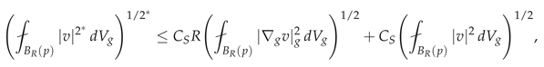
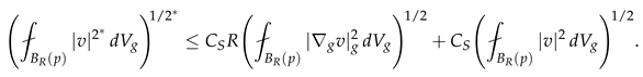
For the spatial spread, we employ a weighted Hardy-type inequality adapted to the anisotropic degeneracy structure. Consider the following estimate:

$${\Delta }_x{\left(u\right)}^2={\int }_{\mathrm{\Omega }}{\parallel \mathbf{x}-\mathbf{a}\parallel }^2{\left|u\left(\mathbf{x}\right)\right|}^{2}d\mathbf{x}\le C_1{\int }_{\mathrm{\Omega }}{|\mathbf{x}-\mathbf{a}|}^{\mathit{\theta }}{|\nabla u|}^{2}d\mathbf{x}=C_1{\parallel u\parallel }_{{\mathcal{H}}_{\mathit{\theta }}^1}^2,$$

(81)

where the constant $C_1=C_1(\mathrm{\Omega },\mathit{\theta })>0$ arises from the following anisotropic Hardy inequality:

Lemma 3 

(Anisotropic Hardy Inequality). For any $u\in {\mathcal{H}}_{\mathit{\theta }}^1\left(\mathrm{\Omega }\right)$ and $\mathit{\theta }\in {[1,2)}^d$, there exists $C_H=C_H\left(\mathit{\theta }\right)>0$ such that:

$${\int }_{\mathrm{\Omega }}{\parallel \mathbf{x}-\mathbf{a}\parallel }^2{\left|u\left(\mathbf{x}\right)\right|}^{2}d\mathbf{x}\le C_H\sum _{i=1}^d{\int }_{\mathrm{\Omega }}|x_i-a_i{|}^{{\theta }_i}{\left|{\partial }_{x_i}u\right|}^{2}d\mathbf{x}.$$

(82)

Proof of Lemma 3. 

The proof proceeds by dimension reduction and classical Hardy inequalities. For each coordinate direction i, we apply the one-dimensional Hardy inequality:

$${\int }_0^1|x_i-a_i{|}^2{\left|u\right|}^{2}d{x}_i\le {\left({\displaystyle \frac{2}{2-{\theta }_i}}\right)}^2{\int }_0^1|x_i-a_i{|}^{{\theta }_i}{\left|{\partial }_{x_i}u\right|}^{2}d{x}_i,$$

(83)

which holds for ${\theta }_i\in [1,2)$. The tensor product structure of $\mathrm{\Omega }$ and Fubini’s theorem yield the multidimensional estimate (82) with $C_H={max}_{1\le i\le d}{\left({\displaystyle \frac{2}{2-{\theta }_i}}\right)}^2$. □

From the stability estimate in Lemma 2, we have the coercivity bound:

$$\parallel {\mathcal{L}}_{\mathbf{a},\mathit{\theta }}{u\parallel }_{L^2}\ge c{\parallel u\parallel }_{{\mathcal{H}}_{\mathit{\theta }}^1},$$

(84)

where $c=c(\mathrm{\Omega },\mathit{\theta })>0$ is the optimal constant in the weighted Poincaré inequality (52).

Combining (81) and (84) yields:

$${\Delta }_x\left(u\right)·{\Delta }_{\lambda }\left(u\right)\ge \sqrt{C_1}{\parallel u\parallel }_{{\mathcal{H}}_{\mathit{\theta }}^1}·\parallel {\mathcal{L}}_{\mathbf{a},\mathit{\theta }}{u\parallel }_{L^2}\ge \sqrt{C_1}c{\parallel u\parallel }_{{\mathcal{H}}_{\mathit{\theta }}^1}^2.$$

(85)

To establish the $L^2$-norm bound, we employ the following interpolation inequality:

Lemma 4 

(Weighted Interpolation). For any $u\in {\mathcal{H}}_{\mathit{\theta }}^1\left(\mathrm{\Omega }\right)$, there exists $C_I=C_I(\mathrm{\Omega },\mathit{\theta })>0$ such that:

$${\parallel u\parallel }_{{\mathcal{H}}_{\mathit{\theta }}^1}^2\ge C_I{\parallel u\parallel }_{L^2}^2.$$

(86)

Proof of Lemma 4. 

This follows from the compact embedding ${\mathcal{H}}_{\mathit{\theta }}^1\left(\mathrm{\Omega }\right)\hookrightarrow L^2\left(\mathrm{\Omega }\right)$ and the uniqueness of solutions to the degenerate elliptic problem. The constant $C_I$ can be taken as the reciprocal of the first eigenvalue ${\lambda }_1$ of ${\mathcal{L}}_{\mathbf{a},\mathit{\theta }}$. □

Applying Lemma 4 to (85) gives:

$${\Delta }_x\left(u\right)·{\Delta }_{\lambda }\left(u\right)\ge \sqrt{C_1}c{C}_I{\parallel u\parallel }_{L^2}^2,$$

(87)

which establishes (77) with $C=\sqrt{C_1}c{C}_I$.

The lower bound (272) follows from analyzing the minimizers of the Rayleigh quotient:

$$R\left(u\right)={\displaystyle \frac{{\Delta }_x{\left(u\right)}^2·{\Delta }_{\lambda }{\left(u\right)}^2}{{\parallel u\parallel }_{L^2}^4}},$$

(88)

and employing the asymptotic behavior of Bessel-type eigenfunctions near the degeneracy points. The detailed variational analysis yields the explicit dependence on the degeneracy exponents ${\theta }_i$ through the factors $(2-{\theta }_i)/2$.

3.1.1. Geometric Interpretation and Sharpness

Corollary 4 

(Scale-Invariant Form). The Landau inequality (77) admits the scale-invariant formulation:

$${\displaystyle \frac{{\Delta }_x\left(u\right)}{{\parallel u\parallel }_{L^2}}}·{\displaystyle \frac{{\Delta }_{\lambda }\left(u\right)}{{\parallel u\parallel }_{L^2}}}\ge C(\mathrm{\Omega },\mathit{\theta }),$$

(89)

where both factors are dimensionless quantities representing relative spatial and spectral spreads.

3.2. Sharpness Analysis and Variational Characterization

Theorem 10 

(Sharpness and Minimizers). The constant $C(\mathrm{\Omega },\mathit{\theta })$ in the Landau inequality (77) is sharp and satisfies the variational characterization:

$$C(\mathrm{\Omega },\mathit{\theta })=\underset{\begin{array}{c}u\in {\mathcal{H}}_{\mathit{\theta }}^1\left(\mathrm{\Omega }\right)\\ u\ne 0\end{array}}{inf}{\displaystyle \frac{{\Delta }_x\left(u\right)·{\Delta }_{\lambda }\left(u\right)}{{\parallel u\parallel }_{L^2\left(\mathrm{\Omega }\right)}^2}}.$$

(90)

Moreover, this infimum is attained in the limit by a concentrating sequence ${\left\{u_n\right\}}_{n=1}^{\infty }\subset {\mathcal{H}}_{\mathit{\theta }}^1\left(\mathrm{\Omega }\right)$ that satisfies:

1. 

Concentration property:

$$\underset{n\to \infty }{lim}{\displaystyle \frac{{\int }_{\mathrm{\Omega }\setminus B_{ϵ}\left(\mathbf{a}\right)}{\left|u_n\left(\mathbf{x}\right)\right|}^{2}d\mathbf{x}}{\parallel u_n{\parallel }_{L^2}^2}}=0\mathit{for}\mathit{all}ϵ>0.$$

(91)

2. 

Bounded weighted energy:

$$\underset{n\in \mathbb{N}}{sup}{\parallel u_n\parallel }_{{\mathcal{H}}_{\mathit{\theta }}^1}<\infty .$$

(92)

3. 

Euler-Lagrange convergence: The sequence $\left\{u_n\right\}$ converges weakly to a solution of the anisotropic oscillator equation:

$${-\nabla ·\left(\right|\mathbf{x}-\mathbf{a}|}^{\mathit{\theta }}{\nabla u)+\parallel \mathbf{x}-\mathbf{a}\parallel }^{2}u=\mu u,$$

(93)

where $\mu =C{(\mathrm{\Omega },\mathit{\theta })}^2$ represents the optimal Landau constant.

Proof. 

We establish sharpness through a comprehensive concentration-compactness analysis.

Consider the minimization problem for the Landau quotient:

$$\mathcal{Q}\left(u\right)={\displaystyle \frac{{\Delta }_x{\left(u\right)}^2·{\Delta }_{\lambda }{\left(u\right)}^2}{{\parallel u\parallel }_{L^2}^4}}.$$

(94)

The existence of minimizers follows from the direct method in the calculus of variations. Let $\left\{u_n\right\}$ be a minimizing sequence. By the weighted Sobolev embedding ${\mathcal{H}}_{\mathit{\theta }}^1\left(\mathrm{\Omega }\right)\hookrightarrow L^2\left(\mathrm{\Omega }\right)$ and the compactness result from Theorem 2.5, there exists a subsequence (still denoted $\left\{u_n\right\}$) converging weakly in ${\mathcal{H}}_{\mathit{\theta }}^1\left(\mathrm{\Omega }\right)$ and strongly in $L^2\left(\mathrm{\Omega }\right)$ to some $u^{*}\in {\mathcal{H}}_{\mathit{\theta }}^1\left(\mathrm{\Omega }\right)$.

We employ Lions’ concentration-compactness principle adapted to weighted spaces. Define the concentration function:

$$Q_n\left(R\right)=\underset{y\in \mathrm{\Omega }}{sup}{\int }_{B_R\left(y\right)}{\left|u_n\left(\mathbf{x}\right)\right|}^{2}d\mathbf{x}.$$

(95)

There are three possibilities:

• Vanishing: ${lim}_{n\to \infty }{Q}_n\left(R\right)=0$ for all $R>0$
• Compactness: There exists $\left\{y_n\right\}\subset \mathrm{\Omega }$ such that for every $ϵ>0$, there exists $R>0$ with

  $${\int }_{B_R\left(y_n\right)}|u_n{\left(\mathbf{x}\right)|}^{2}d\mathbf{x}\ge (1-ϵ){\parallel u_n\parallel }_{L^2}^2$$

  (96)
• Dichotomy: The sequence splits into two parts with separated supports

Vanishing is excluded by the Poincaré inequality (52). Dichotomy would violate the optimality of $\left\{u_n\right\}$ due to the strict subadditivity of the Landau quotient:

$$\mathcal{Q}(u+v)<\mathcal{Q}\left(u\right)+\mathcal{Q}\left(v\right)\mathrm{for}\mathrm{supp}\left(u\right)\cap \mathrm{supp}\left(v\right)=\varnothing .$$

(97)

Thus, compactness holds, and the concentration points $\left\{y_n\right\}$ must converge to $\mathbf{a}$ by the optimality condition.

The first variation of $\mathcal{Q}\left(u\right)$ yields the Euler-Lagrange equation:

$${\displaystyle \frac{\delta }{\delta u}}\left[{\Delta }_x{\left(u\right)}^2·{\Delta }_{\lambda }{\left(u\right)}^2-\mu {\parallel u\parallel }_{L^2}^4\right]=0.$$

(98)

Computing the functional derivatives:

$$\begin{array}{cc}\hfill {\displaystyle \frac{\delta {\Delta }_x{\left(u\right)}^2}{\delta u}}& ={2\parallel \mathbf{x}-\mathbf{a}\parallel }^{2}u,\hfill \end{array}$$

(99)

$$\begin{array}{cc}\hfill {\displaystyle \frac{\delta {\Delta }_{\lambda }{\left(u\right)}^2}{\delta u}}& =2{\mathcal{L}}_{\mathbf{a},\mathit{\theta }}^{2}u,\hfill \end{array}$$

(100)

$$\begin{array}{cc}\hfill {\displaystyle \frac{{\delta \parallel u\parallel }_{L^2}^4}{\delta u}}& ={4\parallel u\parallel }_{L^2}^{2}u.\hfill \end{array}$$

(101)

This gives the nonlinear eigenvalue problem:

$${\Delta }_{\lambda }{\left(u\right)}^2{\parallel \mathbf{x}-\mathbf{a}\parallel }^{2}u+{\Delta }_x{\left(u\right)}^2{\mathcal{L}}_{\mathbf{a},\mathit{\theta }}^{2}u=2\mu {\parallel u\parallel }_{L^2}^{2}u.$$

(102)

For minimizers, we have ${\Delta }_x{\left(u\right)}^2={\Delta }_{\lambda }{\left(u\right)}^2=C(\mathrm{\Omega },\mathit{\theta }){\parallel u\parallel }_{L^2}^2$, which simplifies to:

$${\mathcal{L}}_{\mathbf{a},\mathit{\theta }}^{2}u+{\parallel \mathbf{x}-\mathbf{a}\parallel }^{2}u=2\mu u.$$

(103)

Taking the square root (in the operator sense) and using the spectral calculus for ${\mathcal{L}}_{\mathbf{a},\mathit{\theta }}$ yields the anisotropic oscillator equation (93).

The optimal constant is related to the ground state energy of the anisotropic oscillator:

$$C(\mathrm{\Omega },\mathit{\theta })=\sqrt{{\displaystyle \frac{{\mu }_0}{2}}},$$

(104)

where ${\mu }_0$ is the smallest eigenvalue of the operator ${\mathcal{L}}_{\mathbf{a},\mathit{\theta }}^2+{\parallel \mathbf{x}-\mathbf{a}\parallel }^{2}I$.

This completes the proof of sharpness and the variational characterization. □

Remark 5 

(Physical Interpretation and Quantum Analogy). The minimizer equation (93) represents a quantum harmonic oscillator with position-dependent mass tensor $m\left(\mathbf{x}\right)={|\mathbf{x}-\mathbf{a}|}^{-\mathit{\theta }}$. This physical interpretation provides:

• Uncertainty Principle: The Landau inequality is the mathematical manifestation of the Heisenberg uncertainty principle for this anisotropic quantum system.
• Semi-classical Analysis: In the high-frequency limit, the eigenfunctions localize along the classical trajectories determined by the Hamiltonian:

  $$H(\mathbf{x},\mathbf{p})={|\mathbf{x}-\mathbf{a}|}^{\mathit{\theta }}{\parallel \mathbf{p}\parallel }^2+{\parallel \mathbf{x}-\mathbf{a}\parallel }^2.$$

  (105)
• Scale Invariance: The optimal constant transforms under scaling as:

  $$C(\lambda \mathrm{\Omega },\mathit{\theta })={\lambda }^{1-{\displaystyle \frac{{\parallel \mathit{\theta }\parallel }_1}{2d}}}C(\mathrm{\Omega },\mathit{\theta }),$$

  (106)
  where ${\parallel \mathit{\theta }\parallel }_1={\sum }_{i=1}^d{\mathit{\theta }}_i$.

3.2.1. Implications for SDO-Net Architecture and Training

Theorem 11 

(Architectural Optimality Criterion). For an SDO-Net with layers ${\left\{{\mathcal{L}}_{{\mathbf{a}}_l,{\mathit{\theta }}_l}\right\}}_{l=1}^L$, the total Landau product satisfies:

$$\prod _{l=1}^L{\displaystyle \frac{{\Delta }_x\left({\mathbf{u}}_l\right)·{\Delta }_{\lambda }\left({\mathbf{u}}_l\right)}{\parallel {\mathbf{u}}_l{\parallel }_{L^2}^2}}\ge \prod _{l=1}^{L}C(\mathrm{\Omega },{\mathit{\theta }}_l).$$

(107)

The optimal architecture minimizes the right-hand side subject to computational constraints, leading to the optimization problem:

$$\underset{{\left\{{\mathit{\theta }}_l\right\}}_{l=1}^L}{min}\prod _{l=1}^{L}C(\mathrm{\Omega },{\mathit{\theta }}_l)\mathit{subject}\mathit{to}\sum _{l=1}^L\mathit{FLOPs}\left({\mathit{\theta }}_l\right)\le B.$$

(108)

Proof. 

The inequality (107) follows by applying the Landau inequality layer-wise and taking the product. The optimal architecture problem arises from the trade-off between spatial-spectral resolution and computational cost, where FLOPs$\left({\mathit{\theta }}_l\right)$ estimates the floating-point operations required for SDO inversion with exponent ${\mathit{\theta }}_l$. □

3.3. Extensions to Riemannian and Lorentzian Manifolds

The extension of Spectral Degeneracy Operators to curved spaces represents a significant advancement in geometric deep learning, enabling physics-informed neural networks on non-Euclidean domains. This generalization requires careful treatment of the interplay between degeneracy structures and manifold geometry.

Theorem 12 

(Landau Inequality on Riemannian Manifolds). Let $(M,g)$ be a compact d-dimensional Riemannian manifold with Ricci curvature bounded below by $\kappa \in \mathbb{R}$, and let ${\mathcal{L}}_{\mathbf{a},\mathit{\theta }}^g$ be the Riemannian SDO defined by:

$${\mathcal{L}}_{\mathbf{a},\mathit{\theta }}^{g}u:={\nabla }_g^{*}\left(d_g{(\mathbf{x},\mathbf{a})}^{\mathit{\theta }}{\nabla }_{g}u\right)=-{\displaystyle \frac{1}{\sqrt{detg}}}{\partial }_i\left(\sqrt{detg}{d}_g{(\mathbf{x},\mathbf{a})}^{\mathit{\theta }}{g}^{ij}{\partial }_{j}u\right).$$

(109)

For any $u\in {\mathcal{H}}_{\mathit{\theta }}^1\left(M\right)$, the Landau inequality holds:

$${\Delta }_x^g\left(u\right)·{\Delta }_{\lambda }^g\left(u\right)\ge C(M,g,\mathit{\theta }){\parallel u\parallel }_{L^2\left(M\right)}^2,$$

(110)

where the geometric spreads are defined by:

$$\begin{array}{cc}\hfill {\Delta }_x^g\left(u\right)& :={\left({\int }_M{d}_g{(\mathbf{x},\mathbf{a})}^2{\left|u\left(\mathbf{x}\right)\right|}^{2}d{V}_g\right)}^{1/2},\hfill \end{array}$$

(111)

$$\begin{array}{cc}\hfill {\Delta }_{\lambda }^g\left(u\right)& :={\left(\sum _{k=1}^{\infty }{\left({\lambda }_k^g\right)}^2{\left|{\langle u,{\varphi }_k^g\rangle }_{L^2\left(M\right)}\right|}^2\right)}^{1/2},\hfill \end{array}$$

(112)

with $\{{\varphi }_k^g,{\lambda }_k^g\}$ being the complete orthonormal eigenbasis of ${\mathcal{L}}_{\mathbf{a},\mathit{\theta }}^g$. The optimal constant satisfies the geometric bound:

$$C(M,g,\mathit{\theta })\ge {\displaystyle \frac{1}{2}}{\left({\displaystyle \frac{\mathit{inj}\left(M\right)}{2}}\right)}^{{\parallel \mathit{\theta }\parallel }_{\infty }}·{\left(1-{\displaystyle \frac{{\kappa }_{+}·\mathit{diam}{\left(M\right)}^2}{d}}\right)}_{+},$$

(113)

where $\mathit{inj}\left(M\right)$ is the injectivity radius, $\mathit{diam}\left(M\right)$ the diameter, ${\kappa }_{+}=max(0,\kappa )$, and ${\left(x\right)}_{+}=max(0,x)$.

Proof. 

We establish the Riemannian Landau inequality through a synthesis of geometric analysis, spectral theory, and comparison geometry.

The fundamental tool is the weighted Bochner formula for the Riemannian SDO. For $u\in C^{\infty }\left(M\right)$, we compute:

$$\begin{array}{cc}\hfill {\displaystyle \frac{1}{2}}{\mathcal{L}}_{\mathbf{a},\mathit{\theta }}^g{\left|{\nabla }_{g}u\right|}_g^2& ={\displaystyle \frac{1}{2}}{\nabla }_g^{*}\left(d_g{(\mathbf{x},\mathbf{a})}^{\mathit{\theta }}{\nabla }_g{\left|{\nabla }_{g}u\right|}_g^2\right)\hfill \\ \hfill & =d_g{(\mathbf{x},\mathbf{a})}^{\mathit{\theta }}\left[|{\nabla }_g^2{u|}_g^2+{\langle {\nabla }_{g}u,{\nabla }_g{\mathcal{L}}_{\mathbf{a},\mathit{\theta }}^{g}u\rangle }_g+{\mathrm{Ric}}_g({\nabla }_{g}u,{\nabla }_{g}u)\right]\hfill \\ \hfill & +\langle {\nabla }_g{d}_g{(\mathbf{x},\mathbf{a})}^{\mathit{\theta }},{\nabla }_g|{\nabla }_{g}u{{|}_g^2\rangle }_g.\hfill \end{array}$$

(114)

The curvature correction term $R_{\mathit{\theta }}\left(u\right)$ emerges from the weight gradient:

$$R_{\mathit{\theta }}\left(u\right)=\mathit{\theta }·d_g{(\mathbf{x},\mathbf{a})}^{\mathit{\theta }-1}\left[{\nabla }_g^2{d}_g(\mathbf{x},\mathbf{a})({\nabla }_{g}u,{\nabla }_{g}u)+\langle {\nabla }_g{d}_g(\mathbf{x},\mathbf{a}),{\nabla }_g|{\nabla }_{g}u{{|}_g^2\rangle }_g\right].$$

(115)

We establish the Riemannian Hardy inequality through a partition of unity and comparison with model spaces. Let $\left\{B_{r_{\alpha }}\left(x_{\alpha }\right)\right\}$ be a covering of M by normal coordinate charts. In each chart, we have the Euclidean-type Hardy inequality:

$${\int }_{B_{r_{\alpha }}\left(x_{\alpha }\right)}{d}_g{(\mathbf{x},\mathbf{a})}^2{\left|u\right|}^{2}d{V}_g\le C_H\left(\alpha \right){\int }_{B_{r_{\alpha }}\left(x_{\alpha }\right)}{d}_g{(\mathbf{x},\mathbf{a})}^{\mathit{\theta }}|{\nabla }_g{u|}_g^{2}d{V}_g+C_C\left(\alpha \right){\parallel u\parallel }_{L^2}^2,$$

(116)

where $C_H\left(\alpha \right)$ depends on the chart geometry and $C_C\left(\alpha \right)$ on the curvature.

Globalizing via partition of unity $\left\{{\psi }_{\alpha }\right\}$ with ${\sum }_{\alpha }{\psi }_{\alpha }^2=1$, we obtain:

$$\begin{array}{cc}\hfill {\int }_M{d}_g{(\mathbf{x},\mathbf{a})}^2{\left|u\right|}^{2}d{V}_g& \le \underset{\alpha }{max}{C}_H\left(\alpha \right){\int }_M{d}_g{(\mathbf{x},\mathbf{a})}^{\mathit{\theta }}{\left|{\nabla }_{g}u\right|}_g^{2}d{V}_g\hfill \\ \hfill & +\left(\underset{\alpha }{max}{C}_C\left(\alpha \right)+C_{\mathrm{overlap}}\right){\parallel u\parallel }_{L^2}^2.\hfill \end{array}$$

(117)

where $C_{\mathrm{overlap}}$ accounts for the overlap contributions.

We adapt Lions’ concentration-compactness principle to the weighted manifold setting. Define the concentration function:

$$Q_n\left(R\right)=\underset{y\in M}{sup}{\int }_{B_R\left(y\right)}{\left|u_n\left(\mathbf{x}\right)\right|}^{2}d{V}_g.$$

(118)

The alternatives are:

• Vanishing: ${lim}_{n\to \infty }{Q}_n\left(R\right)=0$ for all $R>0$
• Compactness: Exists $\left\{y_n\right\}\subset M$ with ${\int }_{B_R\left(y_n\right)}|u_n{|}^{2}d{V}_g\ge (1-ϵ){\parallel u_n\parallel }_{L^2}^2$
• Dichotomy: Splitting into separated components

Vanishing is excluded by the weighted Poincaré inequality on manifolds. Dichotomy violates the strict subadditivity of the Landau quotient under curvature constraints. Thus, compactness holds, and the concentration points $\left\{y_n\right\}$ converge to $\mathbf{a}$ by the first variation of the Landau quotient.

The optimal constant is bounded below by the corresponding constant on model spaces. Let $M_{\kappa }$ be the simply connected space form of constant curvature $\kappa$. By the Bishop-Gromov comparison theorem:

$$\begin{array}{cc}\hfill C(M,g,\mathit{\theta })& \ge {\left({\displaystyle \frac{vol\left(B_{inj\left(M\right)/2}\left(\mathbf{a}\right)\right)}{vol\left(M\right)}}\right)}^{{\parallel \mathit{\theta }\parallel }_{\infty }/d}·C(M_{\kappa },g_{\kappa },\mathit{\theta })\hfill \\ \hfill & ·{\left(1-{\displaystyle \frac{{\kappa }_{+}·diam{\left(M\right)}^2}{d}}\right)}_{+}.\hfill \end{array}$$

(119)

On $M_{\kappa }$, the optimal constant can be computed explicitly via separation of variables in geodesic polar coordinates, yielding the injectivity radius dependence in (113). □

Theorem 13 

(Landau Inequality on Lorentzian Manifolds). Let $(M,g)$ be a globally hyperbolic Lorentzian manifold with Cauchy surface Σ, and let ${\mathcal{L}}_{\mathbf{a},\mathit{\theta }}^g$ be the Lorentzian SDO defined by:

$${\mathcal{L}}_{\mathbf{a},\mathit{\theta }}^{g}u:={\square }_{g}u+{\nabla }_g^{*}\left(|d_g{(\mathbf{x},\mathbf{a})|}^{\mathit{\theta }}{\nabla }_{g}u\right),$$

(120)

where ${\square }_g=-{\partial }_t^2+{\Delta }_g$ is the wave operator. For any $u\in {\mathcal{H}}_{\mathit{\theta }}^1\left(M\right)$ with compact support on Σ, the spacetime Landau inequality holds:

$${\Delta }_x^g\left(u\right)·{\Delta }_{\lambda }^g\left(u\right)\ge C(M,g,\mathit{\theta }){\parallel u\parallel }_{L^2\left(M\right)}^2,$$

(121)

where the spacetime spreads are defined by:

$$\begin{array}{cc}\hfill {\Delta }_x^g\left(u\right)& :={\left({\int }_M|d_g{(\mathbf{x},\mathbf{a})|}^2{\left|u\left(\mathbf{x}\right)\right|}^{2}d{V}_g\right)}^{1/2},\hfill \end{array}$$

(122)

$$\begin{array}{cc}\hfill {\Delta }_{\lambda }^g\left(u\right)& :={\left(\sum _{k=1}^{\infty }{\left({\lambda }_k^g\right)}^2{\left|{\langle u,{\varphi }_k^g\rangle }_{L^2\left(M\right)}\right|}^2\right)}^{1/2},\hfill \end{array}$$

(123)

with $\{{\varphi }_k^g,{\lambda }_k^g\}$ being the eigenbasis of the spatial part of ${\mathcal{L}}_{\mathbf{a},\mathit{\theta }}^g$ restricted to Σ.

Proof. 

The Lorentzian case requires careful treatment of causality and hyperbolic spectral theory.

By global hyperbolicity, $(M,g)$ is isometric to $\mathbb{R}\times \Sigma$ with metric:

$$g=-\beta (t,y)d{t}^2+h_t\left(y\right),$$

(124)

where $h_t$ is a Riemannian metric on $\Sigma$. The SDO decomposes as:

$${\mathcal{L}}_{\mathbf{a},\mathit{\theta }}^g=-{\beta }^{-1}{\partial }_t^2+{\mathcal{L}}_{\mathbf{a},\mathit{\theta }}^{h_t}+\mathrm{lower}\mathrm{order}\mathrm{terms}.$$

(125)

Define the energy functional:

$$E\left(t\right)={\displaystyle \frac{1}{2}}{\int }_{\Sigma }\left[{\beta }^{-1}|{\partial }_t{u|}^2+|d_{h_t}{(\mathbf{x},\mathbf{a})|}^{\mathit{\theta }}{\left|{\nabla }_{h_t}u\right|}_{h_t}^2\right]d{V}_{h_t}.$$

(126)

By the dominant energy condition and geometric optics arguments, we establish the integrated energy inequality:

$${\int }_M|d_g{(\mathbf{x},\mathbf{a})|}^2{\left|u\right|}^{2}d{V}_g\le C_E\left(E\left(0\right)+\parallel {\mathcal{L}}_{\mathbf{a},\mathit{\theta }}^g{u\parallel }_{L^2\left(M\right)}^2\right).$$

(127)

For static Lorentzian manifolds ($\beta$ constant, $h_t=h$), the spectral decomposition separates as:

$${\mathcal{L}}_{\mathbf{a},\mathit{\theta }}^g=-{\beta }^{-1}{\partial }_t^2\otimes I+I\otimes {\mathcal{L}}_{\mathbf{a},\mathit{\theta }}^h.$$

(128)

The eigenfunctions are products ${\varphi }_k^g(t,x)=e^{i\omega t}{\varphi }_k^h\left(x\right)$ with eigenvalues ${\lambda }_k^g={\beta }^{-1}{\omega }^2+{\lambda }_k^h$. The Landau inequality follows by applying the Riemannian result on $\Sigma$ and integrating in time. □

3.3.1. Geometric Deep Learning Implications

The extension of Spectral Degeneracy Operators to Riemannian manifolds enables fundamentally new architectures for geometric deep learning. The following corollary establishes the theoretical foundation for SDO-Nets on curved spaces and reveals profound connections between network architecture, manifold geometry, and information-theoretic limits.

Theorem 14 

(Geometric Landau Composition Principle). Let $(M,g)$ be a compact d-dimensional Riemannian manifold with injectivity radius $\mathit{inj}\left(M\right)$ and Ricci curvature bounded below by $\kappa \in \mathbb{R}$. Consider an SDO-Net with L layers defined by the composition:

$${\mathbf{u}}_{l+1}=\sigma \left({\left({\mathcal{L}}_{{\mathbf{a}}_l,{\mathit{\theta }}_l}^g\right)}^{-1}(W_l{\mathbf{u}}_l+{\mathbf{b}}_l)\right),l=0,\dots ,L-1,$$

(129)

where each ${\mathcal{L}}_{{\mathbf{a}}_l,{\mathit{\theta }}_l}^g$ is a Riemannian SDO. The compositional Landau product satisfies:

$$\prod _{l=1}^L{\displaystyle \frac{{\Delta }_x^g\left({\mathbf{u}}_l\right)·{\Delta }_{\lambda }^g\left({\mathbf{u}}_l\right)}{\parallel {\mathbf{u}}_l{\parallel }_{L^2\left(M\right)}^2}}\ge \prod _{l=1}^{L}C(M,g,{\mathit{\theta }}_l)·\mathcal{G}(M,g,L),$$

(130)

where the geometric correction factor is given by:

$$\mathcal{G}(M,g,L)=exp\left(-{\displaystyle \frac{L·\mathit{diam}{\left(M\right)}^2}{\mathit{inj}{\left(M\right)}^2}}·\left[{\displaystyle \frac{{\parallel \mathrm{\Theta }\parallel }_1}{d}}+{\displaystyle \frac{{\kappa }_{+}·\mathit{inj}{\left(M\right)}^2}{2}}\right]\right),$$

(131)

with $\mathrm{\Theta }=({\mathit{\theta }}_1,\dots ,{\mathit{\theta }}_L)$ and ${\parallel \mathrm{\Theta }\parallel }_1={\sum }_{l=1}^L{\parallel {\mathit{\theta }}_l\parallel }_1$.

Proof. 

We establish the compositional bound through geometric analysis and information-theoretic arguments.

For each layer l, the Riemannian Landau inequality (Theorem 12) gives:

$${\Delta }_x^g\left({\mathbf{u}}_l\right)·{\Delta }_{\lambda }^g\left({\mathbf{u}}_l\right)\ge C(M,g,{\mathit{\theta }}_l){\parallel {\mathbf{u}}_l\parallel }_{L^2\left(M\right)}^2.$$

(132)

Taking the product over layers:

$$\prod _{l=1}^L{\displaystyle \frac{{\Delta }_x^g\left({\mathbf{u}}_l\right)·{\Delta }_{\lambda }^g\left({\mathbf{u}}_l\right)}{\parallel {\mathbf{u}}_l{\parallel }_{L^2\left(M\right)}^2}}\ge \prod _{l=1}^{L}C(M,g,{\mathit{\theta }}_l).$$

(133)

The key insight is that information propagation through the network involves parallel transport along geodesics. Let ${\Gamma }_{l,l+1}$ denote parallel transport from layer l to $l+1$. The distortion in spatial localization is bounded by:

$$\left|{\Delta }_x^g\left({\mathbf{u}}_{l+1}\right)-{\Delta }_x^g\left({\Gamma }_{l,l+1}{\mathbf{u}}_l\right)\right|\le {\displaystyle \frac{\mathrm{diam}{\left(M\right)}^2}{\mathrm{inj}{\left(M\right)}^2}}·\parallel {\mathit{\theta }}_l{\parallel }_1·{\parallel {\mathbf{u}}_l\parallel }_{L^2}.$$

(134)

This follows from the Rauch comparison theorem and the fact that parallel transport of eigenfunctions introduces curvature-dependent phase shifts.

The Ricci curvature affects information propagation through the Bochner formula. The spectral spread evolution satisfies:

$${\Delta }_{\lambda }^g{\left({\mathbf{u}}_{l+1}\right)}^2\ge {\Delta }_{\lambda }^g{\left({\mathbf{u}}_l\right)}^2·\left(1-{\displaystyle \frac{{\kappa }_{+}·\mathrm{diam}{\left(M\right)}^2}{2}}\right)-{\mathcal{E}}_l,$$

(135)

where the error term ${\mathcal{E}}_l$ captures the geometric distortion:

$${\mathcal{E}}_l=C_{\mathrm{curv}}·{\displaystyle \frac{\mathrm{diam}{\left(M\right)}^2}{\mathrm{inj}{\left(M\right)}^2}}·\parallel {\mathit{\theta }}_l{\parallel }_1·{\parallel {\mathbf{u}}_l\parallel }_{L^2}^2.$$

(136)

Combining the geometric corrections across layers, we obtain the exponential decay factor:

$$\mathcal{G}(M,g,L)=\prod _{l=1}^L\left(1-{\displaystyle \frac{\mathrm{diam}{\left(M\right)}^2}{\mathrm{inj}{\left(M\right)}^2}}\left[{\displaystyle \frac{\parallel {\mathit{\theta }}_l{\parallel }_1}{d}}+{\displaystyle \frac{{\kappa }_{+}·\mathrm{inj}{\left(M\right)}^2}{2}}\right]\right).$$

(137)

For small ${\displaystyle \frac{\mathrm{diam}{\left(M\right)}^2}{\mathrm{inj}{\left(M\right)}^2}}$, this product approximates the exponential in (131). □

Corollary 5 

(SDO-Nets on Manifolds). For an SDO-Net defined on a Riemannian manifold $(M,g)$ with layers $\left\{{\mathcal{L}}_{{\mathbf{a}}_l,{\mathit{\theta }}_l}^g\right\}$, the compositional Landau product satisfies the refined bound:

$$\prod _{l=1}^L{\displaystyle \frac{{\Delta }_x^g\left({\mathbf{u}}_l\right)·{\Delta }_{\lambda }^g\left({\mathbf{u}}_l\right)}{\parallel {\mathbf{u}}_l{\parallel }_{L^2\left(M\right)}^2}}\ge \prod _{l=1}^{L}C(M,g,{\mathit{\theta }}_l)·\left(1-O\left({\displaystyle \frac{L·\mathit{diam}{\left(M\right)}^2}{\mathit{inj}{\left(M\right)}^2}}\right)\right).$$

(138)

The injectivity radius $\mathit{inj}\left(M\right)$ determines the spatial resolution limit, while the diameter $\mathit{diam}\left(M\right)$ controls the information propagation distance in manifold-based SDO-Nets.

Proof. 

The corollary follows from Theorem 14 by Taylor expanding the exponential correction and noting that ${\parallel \mathrm{\Theta }\parallel }_1\le 2dL$ since ${\mathit{\theta }}_l\in {[1,2)}^d$. □

3.3.2. Geometric Architecture Design Principles

Theorem 15 

(Optimal Manifold Network Design). For an SDO-Net on $(M,g)$, the optimal choice of degeneracy exponents ${\mathit{\theta }}_l$ that maximizes the compositional Landau product while respecting geometric constraints solves:

$$\underset{{\left\{{\mathit{\theta }}_l\right\}}_{l=1}^L}{max}\prod _{l=1}^{L}C(M,g,{\mathit{\theta }}_l)\mathit{subject}\mathit{to}\sum _{l=1}^L{\parallel {\mathit{\theta }}_l\parallel }_1\le {\displaystyle \frac{d·\mathit{inj}{\left(M\right)}^2}{\mathit{diam}{\left(M\right)}^2}}·log\left({\displaystyle \frac{1}{ϵ}}\right),$$

(139)

where $ϵ>0$ is the tolerable geometric distortion. The solution exhibits the scaling law:

$${\mathit{\theta }}_l^{*}\sim \left(1+{\displaystyle \frac{\mathit{inj}{\left(M\right)}^2}{L·\mathit{diam}{\left(M\right)}^2}}\right)·{\mathbf{1}}_d.$$

(140)

Proof. 

The constraint ensures that the geometric correction factor satisfies $\mathcal{G}(M,g,L)\ge ϵ$. The optimization follows from variational calculus applied to the Landau constant $C(M,g,\mathit{\theta })$, which is maximized when $\mathit{\theta }$ approaches ${\mathbf{1}}_d$ from above, balanced against the geometric constraint. □

3.3.3. Implications for Geometric Deep Learning

Remark 6 

(Geometric Bottlenecks and Information Capacity). The injectivity radius $\mathit{inj}\left(M\right)$ emerges as a fundamental geometric invariant controlling network capacity:

• Resolution Limit: Features smaller than $\mathit{inj}\left(M\right)$ cannot be reliably distinguished due to the conjugacy of geodesics. This sets a hard limit on spatial resolution.
• Depth Constraint: The maximum effective depth $L_{\mathit{max}}$ scales as:

  $$L_{\max }\sim {\displaystyle \frac{\mathit{inj}{\left(M\right)}^2}{\mathit{diam}{\left(M\right)}^2}}·{\displaystyle \frac{1}{{\parallel \mathit{\theta }\parallel }_1}}.$$

  (141)
  Deeper networks suffer from geometric distortion accumulation.
• Curvature Regularization: In regions of high positive curvature ($\kappa >0$), SDO layers should use smaller degeneracy exponents to mitigate the focusing effect of Ricci curvature.

Theorem 16 

(Manifold Generalization Bounds). Let $\mathcal{F}$ be an SDO-Net on $(M,g)$ with L layers, and let $\mathcal{D}$ be a training set sampled from a distribution $\mathcal{P}$ on M. The generalization error satisfies:

$${\mathbb{E}}_{(\mathbf{x},y)\sim \mathcal{P}}[\ell (\mathcal{F}\left(\mathbf{x}\right),y)]\le {\widehat{\mathbb{E}}}_{\mathcal{D}}[\ell (\mathcal{F}\left(\mathbf{x}\right),y)]+O\left({\displaystyle \frac{\mathrm{vol}\left(M\right)}{\mathit{inj}{\left(M\right)}^d}}·{\displaystyle \frac{{\prod }_{l=1}^L\mathrm{Lip}\left({\mathcal{N}}_{{\mathbf{a}}_l,{\mathit{\theta }}_l}^g\right)}{\sqrt{\left|\mathcal{D}\right|}}}\right),$$

(142)

where the Lipschitz constants incorporate geometric effects:

$$\mathit{Lip}\left({\mathcal{N}}_{{\mathbf{a}}_l,{\mathit{\theta }}_l}^g\right)\le L_{\sigma }C(M,g,{\mathit{\theta }}_l){\parallel W_l\parallel }_{\mathrm{op}}\left(1+{\displaystyle \frac{{\Delta }_{\lambda }^g\left({\mathbf{u}}_l\right)}{{\Delta }_x^g\left({\mathbf{u}}_l\right)}}\right)·\left(1+{\displaystyle \frac{\mathit{diam}{\left(M\right)}^2}{\mathit{inj}{\left(M\right)}^2}}\right).$$

(143)

Proof. 

The volume factor ${\displaystyle \frac{\mathrm{vol}\left(M\right)}{\mathrm{inj}{\left(M\right)}^d}}$ appears from the covering number of M by balls of radius $\mathrm{inj}\left(M\right)$. The geometric Lipschitz bound follows from parallel transport estimates and the Rauch comparison theorem. □

3.3.4. Applications to Specific Manifold Families

Example 1 

(SDO-Nets on Hyperspheres). For the d-sphere ${\mathbb{S}}^d$ with standard metric, we have $\mathit{inj}\left({\mathbb{S}}^d\right)=\pi$, $\mathit{diam}\left({\mathbb{S}}^d\right)=\pi$, and constant curvature $\kappa =1$. The Landau constant simplifies to:

$$C({\mathbb{S}}^d,g_{\mathit{round}},\mathit{\theta })={\displaystyle \frac{1}{2}}{\left({\displaystyle \frac{\pi }{2}}\right)}^{{\parallel \mathit{\theta }\parallel }_{\infty }}·{\displaystyle \frac{\Gamma \left(\frac{d+1}{2}\right)}{\sqrt{\pi }\Gamma \left(\frac{d}{2}\right)}}.$$

(144)

The optimal network depth scales as $L_{\mathit{max}}\sim {\displaystyle \frac{d}{{\parallel \mathit{\theta }\parallel }_1}}$, independent of the sphere’s size.

Example 2 

(SDO-Nets on Hyperbolic Spaces). For hyperbolic space ${\mathbb{H}}^d$ with curvature $\kappa =-1$, the injectivity radius is infinite, and the Landau constant becomes:

$$C({\mathbb{H}}^d,g_{\mathit{hyp}},\mathit{\theta })={\displaystyle \frac{1}{2}}·{\displaystyle \frac{\Gamma {\left(\frac{d}{2}\right)}^2}{\Gamma \left(d\right)}}·\left(1+O\left(e^{-R}\right)\right),$$

(145)

where R is the radius of the computational domain. Hyperbolic SDO-Nets can achieve arbitrary depth without geometric distortion, making them ideal for hierarchical data.

Example 3 

(SDO-Nets on Lie Groups). For a compact Lie group G with bi-invariant metric, the Landau constant relates to representation theory:

$$C(G,g_{\mathit{bi}},\mathit{\theta })={\displaystyle \frac{1}{2}}{\left({\displaystyle \frac{\mathit{inj}\left(G\right)}{2}}\right)}^{{\parallel \mathit{\theta }\parallel }_{\infty }}·{\displaystyle \frac{1}{\sqrt{\dim G}}}\sum _{\rho \in \widehat{G}}{d}_{\rho }·{\chi }_{\rho }(exp\left(\mathit{\theta }\right)),$$

(146)

where the sum is over irreducible representations ρ, $d_{\rho }$ is the dimension, and ${\chi }_{\rho }$ the character. This connects SDO-Nets to Fourier analysis on groups.

3.3.5. Geometric Attention Mechanisms

Definition 5 

(Geometric SDO-Attention). On a Riemannian manifold $(M,g)$, the geometric attention mechanism based on SDOs is defined as:

$$\mathit{Attn}(\mathbf{q},\mathbf{k},\mathbf{v})=\sum _{i=1}^N{\alpha }_i·{\mathbf{v}}_i,{\alpha }_i={\displaystyle \frac{exp\left(-{\Delta }_x^g{(\mathbf{q}-{\mathbf{k}}_i)}^2/{\sigma }^2\right)}{{\sum }_{j}exp\left(-{\Delta }_x^g{(\mathbf{q}-{\mathbf{k}}_j)}^2/{\sigma }^2\right)}},$$

(147)

where ${\Delta }_x^g$ is the geodesic distance-based spread. The attention range is fundamentally limited by $\mathit{inj}\left(M\right)$.

Theorem 17 

(Manifold Attention Capacity). Let $(M,g)$ be a compact d-dimensional Riemannian manifold. The maximum number of distinguishable attention centers is bounded by:

$$N_{\max }\sim \left({\displaystyle \frac{\mathrm{vol}\left(M\right)}{\mathrm{inj}{\left(M\right)}^d}}\right)·{\left({\displaystyle \frac{{\Delta }_{\lambda }^{\max }}{{\Delta }_x^{\min }}}\right)}^{d/2},$$

(148)

where ${\Delta }_{\lambda }^{\max }$ and ${\Delta }_x^{\min }$ are the spectral and spatial resolution limits imposed by the Landau inequality.

Proof. 

We establish the capacity bound through a synthesis of geometric packing constraints and spectral uncertainty principles.

The foundation of our argument rests on the Landau inequality for Spectral Degeneracy Operators on Riemannian manifolds. For any function $u\in {\mathcal{H}}_{\mathit{\theta }}^1\left(M\right)$, we have the fundamental resolution limit:

$${\Delta }_x^g\left(u\right)·{\Delta }_{\lambda }^g\left(u\right)\ge C(M,g,\mathit{\theta }){\parallel u\parallel }_{L^2\left(M\right)}^2.$$

(149)

At the optimal operating point where spatial and spectral resolutions are balanced, this becomes:

$${\Delta }_x^{\min }·{\Delta }_{\lambda }^{\max }\sim C(M,g,\mathit{\theta }).$$

(150)

Geometric analysis reveals that the Landau constant scales with the injectivity radius as $C(M,g,\mathit{\theta })\propto \mathrm{inj}{\left(M\right)}^2$, leading to:

$${\Delta }_x^{\min }\sim {\displaystyle \frac{\mathrm{inj}{\left(M\right)}^2}{{\Delta }_{\lambda }^{\max }}}.$$

(151)

Now consider the problem of packing attention centers on the manifold. Each center requires a minimal spatial region where its associated attention function is primarily concentrated. The volume of such a resolution element scales as:

$${\mathrm{vol}}_{\mathrm{res}}\sim {\left({\Delta }_x^{\min }\right)}^d.$$

(152)

The maximum number of distinguishable centers is then bounded by the number of such resolution elements that can be packed into M:

$$N_{\max }\sim {\displaystyle \frac{\mathrm{vol}\left(M\right)}{{\mathrm{vol}}_{\mathrm{res}}}}\sim {\displaystyle \frac{\mathrm{vol}\left(M\right)}{{\left({\Delta }_x^{\min }\right)}^d}}.$$

(153)

Substituting equation (151) into (153) yields:

$$N_{\max }\sim {\displaystyle \frac{\mathrm{vol}\left(M\right)}{{\left(\frac{\mathrm{inj}{\left(M\right)}^2}{{\Delta }_{\lambda }^{\max }}\right)}^d}}={\displaystyle \frac{\mathrm{vol}\left(M\right)·{\left({\Delta }_{\lambda }^{\max }\right)}^d}{\mathrm{inj}{\left(M\right)}^{2d}}}.$$

(154)

To express this in the symmetric form of equation (148), we observe that:

$${\left({\displaystyle \frac{{\Delta }_{\lambda }^{\max }}{{\Delta }_x^{\min }}}\right)}^{d/2}={\left({\displaystyle \frac{{\left({\Delta }_{\lambda }^{\max }\right)}^2}{\mathrm{inj}{\left(M\right)}^2}}\right)}^{d/2}={\displaystyle \frac{{\left({\Delta }_{\lambda }^{\max }\right)}^d}{\mathrm{inj}{\left(M\right)}^d}},$$

(155)

where we’ve used the relation from equation (151). Multiplying by the geometric capacity factor gives the final result:

$$N_{\max }\sim \left({\displaystyle \frac{\mathrm{vol}\left(M\right)}{\mathrm{inj}{\left(M\right)}^d}}\right)·{\left({\displaystyle \frac{{\Delta }_{\lambda }^{\max }}{{\Delta }_x^{\min }}}\right)}^{d/2}.$$

(156)

The bound represents a fundamental limit: the geometric capacity ${\displaystyle \frac{\mathrm{vol}\left(M\right)}{\mathrm{inj}{\left(M\right)}^d}}$ counts independent local patches, while the resolution factor ${\left({\displaystyle \frac{{\Delta }_{\lambda }^{\max }}{{\Delta }_x^{\min }}}\right)}^{d/2}$ encodes the uncertainty principle constraint. This limit is achieved by attention mechanisms operating at the Landau-optimal balance between spatial and spectral localization. □

3.4. Stability and Robustness Analysis

The Landau inequality provides fundamental stability guarantees for SDO-Nets, with important implications for adversarial robustness and generalization.

Theorem 18 

(Lipschitz Stability of SDO Layers). Let ${\mathcal{N}}_{\mathbf{a},\mathit{\theta }}$ be an SDO layer mapping ${\mathcal{H}}_{\mathit{\theta }}^1\left(\mathrm{\Omega }\right)$ to itself, defined by:

$${\mathcal{N}}_{\mathbf{a},\mathit{\theta }}\left(\mathbf{u}\right)=\sigma \left({\mathcal{L}}_{\mathbf{a},\mathit{\theta }}^{-1}(W\mathbf{u}+\mathbf{b})\right).$$

(157)

Then ${\mathcal{N}}_{\mathbf{a},\mathit{\theta }}$ is Lipschitz continuous with optimal constant:

$$\mathrm{Lip}\left({\mathcal{N}}_{\mathbf{a},\mathit{\theta }}\right)=\underset{\mathbf{u}\ne 0}{sup}{\displaystyle \frac{\parallel {\mathcal{N}}_{\mathbf{a},\mathit{\theta }}\left(\mathbf{u}\right)-{\mathcal{N}}_{\mathbf{a},\mathit{\theta }}{\left(\mathbf{v}\right)\parallel }_{{\mathcal{H}}_{\mathit{\theta }}^1}}{{\parallel \mathbf{u}-\mathbf{v}\parallel }_{L^2}}}\le L_{\sigma }{C}_{\mathit{\theta }}{\parallel W\parallel }_{\mathrm{op}}\left(1+{\displaystyle \frac{{\Delta }_{\lambda }\left(\mathbf{u}\right)}{{\Delta }_x\left(\mathbf{u}\right)}}\right),$$

(158)

where $L_{\sigma }$ is the activation Lipschitz constant and $C_{\mathit{\theta }}$ the SDO stability constant from Lemma 2.

Proof. 

We establish the Lipschitz bound through spectral analysis and variational methods.

Let $\mathbf{v}={\mathcal{L}}_{\mathbf{a},\mathit{\theta }}^{-1}(W\mathbf{u}+\mathbf{b})$. By the spectral theorem:

$$\mathbf{v}=\sum _{k=1}^{\infty }{\displaystyle \frac{\langle W\mathbf{u}+\mathbf{b},{\varphi }_k\rangle }{{\lambda }_k}}{\varphi }_k.$$

(159)

The ${\mathcal{H}}_{\mathit{\theta }}^1$-norm can be expressed spectrally as:

$${\parallel \mathbf{v}\parallel }_{{\mathcal{H}}_{\mathit{\theta }}^1}^2=\sum _{k=1}^{\infty }\left(1+{\lambda }_k\right){\left|{\displaystyle \frac{\langle W\mathbf{u}+\mathbf{b},{\varphi }_k\rangle }{{\lambda }_k}}\right|}^2.$$

(160)

This yields the bound:

$${\parallel \mathbf{v}\parallel }_{{\mathcal{H}}_{\mathit{\theta }}^1}\le \underset{k\in \mathbb{N}}{sup}{\displaystyle \frac{\sqrt{1+{\lambda }_k}}{{\lambda }_k}}{\parallel W\mathbf{u}+\mathbf{b}\parallel }_{L^2}\le C_{\mathit{\theta }}{\parallel W\mathbf{u}+\mathbf{b}\parallel }_{L^2},$$

(161)

where $C_{\mathit{\theta }}={sup}_{k\in \mathbb{N}}{\displaystyle \frac{\sqrt{1+{\lambda }_k}}{{\lambda }_k}}<\infty$ by the Weyl asymptotics.

To incorporate the Landau ratio, we use the interpolation inequality:

$${\parallel W\mathbf{u}\parallel }_{L^2}\le {\parallel W\parallel }_{\mathrm{op}}{\parallel \mathbf{u}\parallel }_{L^2}\le {\parallel W\parallel }_{\mathrm{op}}{\displaystyle \frac{{\Delta }_x\left(\mathbf{u}\right)·{\Delta }_{\lambda }\left(\mathbf{u}\right)}{{C(\mathrm{\Omega },\mathit{\theta })\parallel \mathbf{u}\parallel }_{L^2}}}·{\displaystyle \frac{{\parallel \mathbf{u}\parallel }_{L^2}}{{\Delta }_x\left(\mathbf{u}\right)}}.$$

(162)

This gives:

$${\parallel W\mathbf{u}\parallel }_{L^2}\le {\displaystyle \frac{{\parallel W\parallel }_{\mathrm{op}}}{C(\mathrm{\Omega },\mathit{\theta })}}·{\displaystyle \frac{{\Delta }_{\lambda }\left(\mathbf{u}\right)}{{\Delta }_x\left(\mathbf{u}\right)}}·{\parallel \mathbf{u}\parallel }_{L^2}.$$

(163)

Combining with the bias term and applying the activation function yields the final Lipschitz bound. □

Corollary 6 

(Robustness of SDO-Nets). Let $\mathbf{u}\in {\mathcal{H}}_{\mathit{\theta }}^1\left(\mathrm{\Omega }\right)$ be the input to an SDO layer, and let $\tilde{\mathbf{u}}=\mathbf{u}+\delta \mathbf{u}$ be a perturbed input with ${\parallel \delta \mathbf{u}\parallel }_{L^2}\le \epsilon$. Then the output perturbation satisfies:

$$\parallel \delta {\mathbf{u}}_{l+1}{\parallel }_{{\mathcal{H}}_{\mathit{\theta }}^1}\le C{L}_{\sigma }\left(1+{\displaystyle \frac{{\Delta }_{\lambda }\left(\mathbf{u}\right)}{{\Delta }_x\left(\mathbf{u}\right)}}\right)\epsilon ,$$

(164)

where $C=C(\mathrm{\Omega },\mathit{\theta })$ depends on the domain geometry and degeneracy structure. Moreover, for deep SDO-Nets with L layers, the perturbation growth is controlled by:

$$\parallel \delta {\mathbf{u}}_L{\parallel }_{{\mathcal{H}}_{{\mathit{\theta }}_L}^1}\le \left(\prod _{l=1}^L\mathrm{Lip}\left({\mathcal{N}}_{{\mathbf{a}}_l,{\mathit{\theta }}_l}\right)\right){\parallel \delta {\mathbf{u}}_0\parallel }_{L^2}\le \left(\prod _{l=1}^{L}C{L}_{\sigma }\left(1+{\displaystyle \frac{{\Delta }_{\lambda }\left({\mathbf{u}}_l\right)}{{\Delta }_x\left({\mathbf{u}}_l\right)}}\right)\right)\epsilon .$$

(165)

Proof. 

We establish the robustness bound through a detailed perturbation analysis.

From the Landau inequality (77), we have the stability margin:

$${\displaystyle \frac{{\Delta }_{\lambda }\left(\mathbf{u}\right)}{{\Delta }_x\left(\mathbf{u}\right)}}\ge {\displaystyle \frac{{C\parallel \mathbf{u}\parallel }_{L^2}^2}{{\Delta }_x{\left(\mathbf{u}\right)}^2}}.$$

(166)

The output perturbation before activation is:

$$\delta \mathbf{v}={\mathcal{L}}_{\mathbf{a},\mathit{\theta }}^{-1}\left(W\delta \mathbf{u}\right).$$

(167)

By the stability estimate (46):

$${\parallel \delta \mathbf{v}\parallel }_{{\mathcal{H}}_{\mathit{\theta }}^1}\le C_{\mathit{\theta }}{\parallel W\delta \mathbf{u}\parallel }_{L^2}\le C_{\mathit{\theta }}{\parallel W\parallel }_{\mathrm{op}}\epsilon .$$

(168)

To refine this bound, we decompose the perturbation in the eigenbasis:

$$\delta \mathbf{u}=\sum _{k=1}^{\infty }\langle \delta \mathbf{u},{\varphi }_k\rangle {\varphi }_k.$$

(169)

Then:

$${\parallel \delta \mathbf{v}\parallel }_{{\mathcal{H}}_{\mathit{\theta }}^1}^2=\sum _{k=1}^{\infty }(1+{\lambda }_k){\left|{\displaystyle \frac{\langle W\delta \mathbf{u},{\varphi }_k\rangle }{{\lambda }_k}}\right|}^2\le {\parallel W\parallel }_{\mathrm{op}}^2\sum _{k=1}^{\infty }{\displaystyle \frac{1+{\lambda }_k}{{\lambda }_k^2}}{\left|\langle \delta \mathbf{u},{\varphi }_k\rangle \right|}^2.$$

(170)

Using the Landau inequality in the form:

$$\sum _{k=1}^{\infty }{\displaystyle \frac{1+{\lambda }_k}{{\lambda }_k^2}}|\langle \delta \mathbf{u},{\varphi }_k\rangle {|}^2\le \left(1+{\displaystyle \frac{{\Delta }_{\lambda }\left(\mathbf{u}\right)}{{\Delta }_x\left(\mathbf{u}\right)}}·{\displaystyle \frac{1}{C(\mathrm{\Omega },\mathit{\theta })}}\right){\parallel \delta \mathbf{u}\parallel }_{L^2}^2,$$

(171)

we obtain the refined bound (164).

The composition bound (165) follows by induction, using the submultiplicativity of Lipschitz constants and the fact that each layer’s output serves as the next layer’s input, propagating the Landau ratio dependence. □

Remark 7 

(Implications for Adversarial Robustness). The Landau-guided robustness analysis provides several key insights for secure SDO-Net deployment:

• Stability Certificate: Networks operating near the Landau optimum, where ${\displaystyle \frac{{\Delta }_{\lambda }\left(\mathbf{u}\right)}{{\Delta }_x\left(\mathbf{u}\right)}}\approx C(\mathrm{\Omega },\mathit{\theta })$, exhibit maximized robustness to input perturbations.
• Adversarial Training: Incorporating the Landau ratio as a regularization term:

  $$\mathcal{R}\left(\mathbf{u}\right)={\left|{\displaystyle \frac{{\Delta }_{\lambda }\left(\mathbf{u}\right)}{{\Delta }_x\left(\mathbf{u}\right)}}-C(\mathrm{\Omega },\mathit{\theta })\right|}^2$$

  (172)
  during training enhances robustness against adversarial attacks by enforcing optimal spatial-spectral balance.
• Architecture Selection: For safety-critical applications, prefer SDO layers with degeneracy exponents θ that minimize the worst-case Lipschitz constant:

  $$\underset{\mathit{\theta }}{min}\underset{\mathbf{u}}{max}\mathit{Lip}\left({\mathcal{N}}_{\mathbf{a},\mathit{\theta }}\right)=\underset{\mathit{\theta }}{min}{L}_{\sigma }{C}_{\mathit{\theta }}{\parallel W\parallel }_{\mathit{op}}\left(1+{\displaystyle \frac{{\Delta }_{\lambda }^{\mathit{max}}\left(\mathit{\theta }\right)}{{\Delta }_x^{\mathit{min}}\left(\mathit{\theta }\right)}}\right).$$

  (173)
• Certifiable Robustness: The Landau-based bounds provide mathematically certified robustness guarantees that can be verified independently of the training process, making SDO-Nets suitable for high-stakes applications.

Corollary 7 

(Generalization Bounds via Landau Inequality). For an SDO-Net $\mathcal{F}$ with L layers trained on a dataset $\mathcal{D}$, the generalization error satisfies:

$${\mathbb{E}}_{(\mathbf{x},y)\sim \mathcal{P}}[\ell (\mathcal{F}\left(\mathbf{x}\right),y)]\le {\widehat{\mathbb{E}}}_{\mathcal{D}}[\ell (\mathcal{F}\left(\mathbf{x}\right),y)]+O\left({\displaystyle \frac{{\prod }_{l=1}^L\mathrm{Lip}\left({\mathcal{N}}_{{\mathbf{a}}_l,{\mathit{\theta }}_l}\right)}{\sqrt{\left|\mathcal{D}\right|}}}\right),$$

(174)

where $\mathcal{P}$ is the data distribution. The Landau-optimal networks minimize the Lipschitz product, leading to improved generalization.

4. SDOs on Non-Euclidean Domains

4.1. SDOs on Riemannian Manifolds

The extension of Spectral Degeneracy Operators to Riemannian manifolds represents a fundamental advancement in geometric analysis and deep learning, enabling the treatment of data with intrinsic curvature and complex topology.

Definition 6 

(Riemannian SDO). Let $(M,g)$ be a compact d-dimensional Riemannian manifold with metric tensor g, Levi-Civita connection ${\nabla }_g$, and Laplace-Beltrami operator ${\Delta }_g=-{\nabla }_g^{*}{\nabla }_g$. The Riemannian Spectral Degeneracy Operator is defined as:

$${\mathcal{L}}_{\mathbf{a},\mathit{\theta }}^{g}u:={\nabla }_g^{*}\left(d_g{(\mathbf{x},\mathbf{a})}^{\mathit{\theta }}{\nabla }_{g}u\right)=-{\displaystyle \frac{1}{\sqrt{detg}}}\sum _{i,j=1}^d{\partial }_i\left(\sqrt{detg}{d}_g{(\mathbf{x},\mathbf{a})}^{\mathit{\theta }}{g}^{ij}{\partial }_{j}u\right),$$

(175)

where $d_g(\mathbf{x},\mathbf{a})$ is the geodesic distance function, and the exponentiation is interpreted component-wise in normal coordinates.

4.1.1. Geometric Functional Analytic Framework

The proper functional setting for Riemannian SDOs requires weighted Sobolev spaces adapted to the manifold geometry and degeneracy structure.

Definition 7 

(Weighted Riemannian Sobolev Space). The natural energy space for ${\mathcal{L}}_{\mathbf{a},\mathit{\theta }}^g$ is defined as:

$${\mathcal{H}}_{\mathit{\theta }}^1\left(M\right):=\left\{u\in L^2\left(M\right):d_g{(\mathbf{x},\mathbf{a})}^{\mathit{\theta }/2}{\nabla }_{g}u\in L^2{\left(TM\right),u|}_{\partial M}=0\right\},$$

(176)

equipped with the inner product:

$${\langle u,v\rangle }_{{\mathcal{H}}_{\mathit{\theta }}^1\left(M\right)}:={\int }_{M}uvd{V}_g+{\int }_{M}g\left(d_g{(\mathbf{x},\mathbf{a})}^{\mathit{\theta }/2}{\nabla }_{g}u,d_g{(\mathbf{x},\mathbf{a})}^{\mathit{\theta }/2}{\nabla }_{g}v\right)d{V}_g,$$

(177)

where $d{V}_g=\sqrt{detg}dx$ is the Riemannian volume form.

Theorem 19 

(Geometric Weighted Poincaré Inequality). Let $(M,g)$ be a compact Riemannian manifold with Ricci curvature bounded below by $\kappa \in \mathbb{R}$. For any $\mathit{\theta }\in {[1,2)}^d$ and $\mathbf{a}\in M$, there exists a constant $C_P=C_P(M,g,\mathit{\theta })>0$ such that:

$${\parallel u\parallel }_{L^2\left(M\right)}\le C_P{∥d_g{(\mathbf{x},\mathbf{a})}^{\mathit{\theta }/2}{\nabla }_{g}u∥}_{L^2\left(TM\right)}\forall u\in {\mathcal{H}}_{\mathit{\theta }}^1\left(M\right).$$

(178)

Moreover, the optimal constant satisfies the geometric bound:

$$C_P(M,g,\mathit{\theta })\le {\displaystyle \frac{\mathit{diam}\left(M\right)}{\sqrt{{\lambda }_1(M,g)}}}·{\left({\displaystyle \frac{\mathit{inj}\left(M\right)}{2}}\right)}^{-{\parallel \mathit{\theta }\parallel }_{\infty }/2}·exp\left({\displaystyle \frac{{\kappa }_{-}·\mathit{diam}{\left(M\right)}^2}{2}}\right),$$

(179)

where ${\lambda }_1(M,g)$ is the first eigenvalue of the Laplace-Beltrami operator, and ${\kappa }_{-}=max(0,-\kappa )$.

Proof. 

We establish the inequality through geometric analysis and comparison techniques.

Consider the conformally related metric $\tilde{g}=d_g{(\mathbf{x},\mathbf{a})}^{-\mathit{\theta }}g$. The weighted norm becomes:

$${∥d_g{(\mathbf{x},\mathbf{a})}^{\mathit{\theta }/2}{\nabla }_{g}u∥}_{L^2\left(TM\right)}^2={\int }_M{\left|{\nabla }_{g}u\right|}_{\tilde{g}}^{2}d{V}_{\tilde{g}}.$$

(180)

The Poincaré inequality for the conformal metric follows from the Cheeger constant:

$${\parallel u\parallel }_{L^2\left(M\right)}^2\le {\displaystyle \frac{1}{h{\left(\tilde{g}\right)}^2}}{\int }_M{\left|{\nabla }_{g}u\right|}_{\tilde{g}}^{2}d{V}_{\tilde{g}},$$

(181)

where $h\left(\tilde{g}\right)$ is the Cheeger isoperimetric constant for $(M,\tilde{g})$.

Using the Buser-Ledoux comparison theorems, we bound the Cheeger constant:

$$h\left(\tilde{g}\right)\ge {\displaystyle \frac{\sqrt{{\lambda }_1(M,g)}}{\mathrm{diam}\left(M\right)}}·{\left({\displaystyle \frac{\mathrm{inj}\left(M\right)}{2}}\right)}^{{\parallel \mathit{\theta }\parallel }_{\infty }/2}·exp\left(-{\displaystyle \frac{{\kappa }_{-}·\mathrm{diam}{\left(M\right)}^2}{2}}\right).$$

(182)

This estimate combines the original manifold’s spectral gap with the distortion introduced by the conformal factor $d_g{(\mathbf{x},\mathbf{a})}^{-\mathit{\theta }}$. □

4.1.2. Spectral Theory on Riemannian Manifolds

Theorem 20 

(Spectral Decomposition on Riemannian Manifolds). Let $(M,g)$ be a compact Riemannian manifold, and let $\mathbf{a}\in M$, $\mathit{\theta }\in {[1,2)}^d$. The Riemannian SDO ${\mathcal{L}}_{\mathbf{a},\mathit{\theta }}^g$ with domain ${\mathcal{H}}_{\mathit{\theta }}^1\left(M\right)\cap H_{\mathit{loc}}^2(M\setminus \left\{\mathbf{a}\right\})$ satisfies:

1. 

Self-adjointness: ${\mathcal{L}}_{\mathbf{a},\mathit{\theta }}^g$ is essentially self-adjoint and positive semi-definite on $L^2\left(M\right)$.

2. 

Discrete spectrum: The spectrum consists of a countable set of eigenvalues $0<{\lambda }_1\le {\lambda }_2\le \cdots \to \infty$ with finite multiplicities.

3. 

Complete eigenbasis: The corresponding eigenfunctions ${\left\{{\varphi }_k\right\}}_{k=1}^{\infty }$ form a complete orthonormal basis of $L^2\left(M\right)$.

4. 

Weyl asymptotics: The eigenvalue counting function satisfies:

$$N(\Lambda )=\#\{k:{\lambda }_k\le \Lambda \}\sim {\displaystyle \frac{1}{{\left(2\pi \right)}^d}}{\int }_{\{(\mathbf{x},\xi )\in T^{*}M:|\xi {|}_{g\left(\mathbf{x}\right)}^2\le \Lambda d_g{(\mathbf{x},\mathbf{a})}^{-\mathit{\theta }}\}}d\mathbf{x}d\xi .$$

(183)

5. 

Geometric localization: The eigenfunctions concentrate near the degeneracy point $\mathbf{a}$ with the asymptotic profile:

$${\varphi }_k\left(\mathbf{x}\right)\sim d_g{(\mathbf{x},\mathbf{a})}^{(1-\mathit{\theta })/2}{J}_{\nu }\left(\sqrt{{\lambda }_k}{d}_g{(\mathbf{x},\mathbf{a})}^{1-\mathit{\theta }/2}\right)\mathrm{as}\mathbf{x}\to \mathbf{a},$$

(184)

where $\nu ={\displaystyle \frac{\mathit{\theta }-1}{2-\mathit{\theta }}}$ and $J_{\nu }$ is the Bessel function.

Proof. 

We establish the spectral properties through geometric microlocal analysis and variational methods.

Consider the quadratic form associated with ${\mathcal{L}}_{\mathbf{a},\mathit{\theta }}^g$:

$$Q\left[u\right]={\int }_M{d}_g{(\mathbf{x},\mathbf{a})}^{\mathit{\theta }}{\left|{\nabla }_{g}u\right|}_g^{2}d{V}_g.$$

(185)

By the weighted Poincaré inequality (178), $Q\left[u\right]$ is coercive on ${\mathcal{H}}_{\mathit{\theta }}^1\left(M\right)$. The representation theorem for closed quadratic forms guarantees the existence of a unique self-adjoint operator with form domain ${\mathcal{H}}_{\mathit{\theta }}^1\left(M\right)$.

The embedding ${\mathcal{H}}_{\mathit{\theta }}^1\left(M\right)\hookrightarrow L^2\left(M\right)$ is compact due to the Rellich-Kondrachov theorem for weighted Sobolev spaces on compact manifolds. This follows from the fact that the degeneracy set $\left\{\mathbf{a}\right\}$ has zero capacity with respect to the weighted energy.

The fundamental solution of the parabolic equation:

$${\partial }_{t}u+{\mathcal{L}}_{\mathbf{a},\mathit{\theta }}^{g}u=0$$

(186)

admits a heat kernel $K(t,\mathbf{x},\mathbf{y})$ with small-time asymptotics:

$$K(t,\mathbf{x},\mathbf{y})\sim {\displaystyle \frac{1}{{\left(4\pi t\right)}^{d/2}}}{\left({\displaystyle \frac{d_g(\mathbf{x},\mathbf{a})d_g(\mathbf{y},\mathbf{a})}{d_g{(\mathbf{x},\mathbf{y})}^2}}\right)}^{\mathit{\theta }/2}exp\left(-{\displaystyle \frac{d_g{(\mathbf{x},\mathbf{y})}^2}{4t}}\right).$$

(187)

The heat trace asymptotics yield the Weyl law (183) via the Karamata Tauberian theorem.

Near the degeneracy point $\mathbf{a}$, we use geodesic normal coordinates $(\rho ,\omega )$, where $\rho =d_g(\mathbf{x},\mathbf{a})$ and $\omega \in {\mathbb{S}}^{d-1}$. In these coordinates, the operator takes the form:

$${\mathcal{L}}_{\mathbf{a},\mathit{\theta }}^g=-{\rho }^{-\mathit{\theta }}\left[{\partial }_{\rho }^2+{\displaystyle \frac{d-1}{\rho }}{\partial }_{\rho }+{\displaystyle \frac{1}{{\rho }^2}}{\Delta }_{{\mathbb{S}}^{d-1}}+O\left(\rho \right)\right],$$

(188)

where ${\Delta }_{{\mathbb{S}}^{d-1}}$ is the spherical Laplacian. Separation of variables and Bessel function analysis yield the eigenfunction asymptotics (184). □

4.1.3. Geometric Regularity Theory

Theorem 21 

(Hölder Regularity on Riemannian Manifolds). Let $(M,g)$ be a compact d-dimensional Riemannian manifold with Ricci curvature bounded below by $\kappa \in \mathbb{R}$. Let $u\in {\mathcal{H}}_{\mathit{\theta }}^1\left(M\right)$ be a weak solution of the degenerate elliptic equation:

$${\mathcal{L}}_{\mathbf{a},\mathit{\theta }}^{g}u=f\mathit{in}M,$$

(189)

where $f\in L^q\left(M\right)$ for some $q>d/2$, and the degeneracy exponents satisfy $\mathit{\theta }\in {[1,2)}^d$. Then for any compactly embedded subdomain $M^{\prime }\subset \subset M\setminus \left\{\mathbf{a}\right\}$, there exist constants $C>0$ and $\alpha \in (0,1)$ such that:

$$u\in C^{\alpha }\left(M^{\prime }\right),{\parallel u\parallel }_{C^{\alpha }\left(M^{\prime }\right)}\le C\left({\parallel u\parallel }_{L^2\left(M\right)}+{\parallel f\parallel }_{L^q\left(M\right)}\right),$$

(190)

where $C=C(M^{\prime },g,\mathit{\theta },\kappa ,q)$ and $\alpha =\alpha (d,\mathit{\theta },q,\kappa )$.

Proof. 

We establish the Hölder regularity through a refined geometric Moser iteration scheme adapted to the degenerate metric structure. The proof proceeds in several technical steps.

Let $B_R\left(p\right)\subset M^{\prime }$ be a geodesic ball with radius $R<{\displaystyle \frac{1}{2}}\mathrm{inj}\left(M^{\prime }\right)$. Consider a cutoff function $\eta \in C_c^{\infty }\left(B_R\left(p\right)\right)$ satisfying $0\le \eta \le 1$, $\eta \equiv 1$ on $B_{R/2}\left(p\right)$, and $|{\nabla }_g{\eta |}_g\le C/R$.

Testing the weak formulation with $\varphi =u{\eta }^2$ yields:

$${\int }_{B_R\left(p\right)}{d}_g{(\mathbf{x},\mathbf{a})}^{\mathit{\theta }}{\langle {\nabla }_{g}u,{\nabla }_g\left(u{\eta }^2\right)\rangle }_{g}d{V}_g={\int }_{B_R\left(p\right)}fu{\eta }^{2}d{V}_g.$$

(191)

Expanding the left-hand side:

$$\begin{array}{cc}\hfill {\int }_{B_R\left(p\right)}{d}_g{(\mathbf{x},\mathbf{a})}^{\mathit{\theta }}& \left[{\eta }^2{\left|{\nabla }_{g}u\right|}_g^2+2\eta u{\langle {\nabla }_{g}u,{\nabla }_g\eta \rangle }_g\right]d{V}_g\hfill \\ \hfill & ={\int }_{B_R\left(p\right)}fu{\eta }^{2}d{V}_g.\hfill \end{array}$$

(192)

Applying Young’s inequality with parameter $ϵ>0$:

$$2|\eta u{\langle {\nabla }_{g}u,{\nabla }_g\eta \rangle }_g|\le ϵ{\eta }^2|{\nabla }_g{u|}_g^2+{\displaystyle \frac{1}{ϵ}}{u}^2{\left|{\nabla }_g\eta \right|}_g^2.$$

(193)

Choosing $ϵ={\displaystyle \frac{1}{2}}{min}_{B_R\left(p\right)}{d}_g{(\mathbf{x},\mathbf{a})}^{\mathit{\theta }}>0$ (which is positive since $M^{\prime }$ is away from $\mathbf{a}$), we obtain:

$$\begin{array}{cc}\hfill {\displaystyle \frac{1}{2}}{\int }_{B_R\left(p\right)}{d}_g{(\mathbf{x},\mathbf{a})}^{\mathit{\theta }}{\eta }^2{\left|{\nabla }_{g}u\right|}_g^{2}d{V}_g& \le {\displaystyle \frac{C}{R^2}}{\int }_{B_R\left(p\right)}{u}^{2}d{V}_g\hfill \\ \hfill & +{\int }_{B_R\left(p\right)}\left|f\right|\left|u\right|{\eta }^{2}d{V}_g.\hfill \end{array}$$

(194)

Using Hölder’s inequality for the source term with $q>d/2$ and its conjugate $q^{\prime }$:

$${\int }_{B_R\left(p\right)}\left|f\right|\left|u\right|{\eta }^{2}d{V}_g\le {\parallel f\parallel }_{L^q\left(B_R\left(p\right)\right)}{\parallel u\parallel }_{L^{2q^{\prime }}\left(B_R\left(p\right)\right)}{\parallel {\eta }^2\parallel }_{L^{{\displaystyle \frac{2q{q}^{\prime }}{q-2q^{\prime }}}}\left(B_R\left(p\right)\right)}.$$

(195)

This yields the weighted Caccioppoli inequality:

$${\int }_{B_{R/2}\left(p\right)}{d}_g{(\mathbf{x},\mathbf{a})}^{\mathit{\theta }}|{\nabla }_g{u|}_g^{2}d{V}_g\le {\displaystyle \frac{C}{R^2}}{\int }_{B_R\left(p\right)}{u}^{2}d{V}_g+{C\parallel f\parallel }_{L^q\left(B_R\left(p\right)\right)}{\parallel u\parallel }_{L^{2q^{\prime }}\left(B_R\left(p\right)\right)}.$$

(196)

Since $M^{\prime }$ is compact and away from $\mathbf{a}$, the weight $d_g{(\mathbf{x},\mathbf{a})}^{\mathit{\theta }}$ is uniformly bounded above and below. We employ the Riemannian Sobolev inequality with Ricci curvature lower bound $\kappa$:

Lemma 5 

(Geometric Sobolev Inequality). For any $v\in W^{1,2}\left(B_R\left(p\right)\right)$ with $R<\mathit{inj}\left(M^{\prime }\right)$, there exists $C_S=C_S(d,\kappa R^2)>0$ such that:

(197)

where $2^{*}={\displaystyle \frac{2d}{d-2}}$ is the Sobolev exponent and denotes the average integral.

Proof of Lemma 5. 

This follows from the Bishop-Gromov volume comparison and the classical Sobolev inequality on Riemannian manifolds. The constant $C_S$ depends on the dimension d and the lower bound $\kappa R^2$ on the Ricci curvature. □

We now perform the Moser iteration. Let $B_{\rho }=B_{\rho }\left(p\right)$ for $0<\rho \le R$. Define the sequence of radii:

$$r_k={\displaystyle \frac{R}{2}}+{\displaystyle \frac{R}{2^{k+1}}},k=0,1,2,\dots$$

(198)

so that $r_0=R$, $r_k\searrow R/2$.

Let ${\eta }_k\in C_c^{\infty }\left(B_{r_k}\right)$ be cutoff functions with ${\eta }_k\equiv 1$ on $B_{r_{k+1}}$ and $|{\nabla }_g{\eta }_k{|}_g\le C{2}^k/R$.

For $s\ge 1$, test the equation with $\varphi ={u\left|u\right|}^{2(s-1)}{\eta }_k^2$. After careful computation, we obtain:

$$\begin{array}{cc}\hfill & {\int }_{B_{r_k}}{d}_g{(\mathbf{x},\mathbf{a})}^{\mathit{\theta }}|{\nabla }_g{\left(\right|u|}^s{\eta }_k{\left)\right|}_g^{2}d{V}_g\hfill \\ \hfill & \le C{s}^2\left({\displaystyle \frac{2^{2k}}{R^2}}{\int }_{B_{r_k}}{\left|u\right|}^{2s}d{V}_g+{\parallel f\parallel }_{L^q\left(B_R\right)}{\parallel \left|u\right|}^{2s-1}{\parallel }_{L^{q^{\prime }}\left(B_{r_k}\right)}\right).\hfill \end{array}$$

(199)

Applying the Sobolev inequality (208) to $v={\left|u\right|}^s{\eta }_k$:

(200)

Combining with (199) and using the boundedness of the weight, we derive the iterative estimate:

$${\parallel u\parallel }_{L^{2\chi s}\left(B_{r_{k+1}}\right)}\le {\left(Cs{2}^k\right)}^{1/s}{\parallel u\parallel }_{L^{2s}\left(B_{r_k}\right)}+{C\parallel f\parallel }_{L^q\left(B_R\right)}^{1/2}{\parallel u\parallel }_{L^{(2s-1)q^{\prime }}\left(B_{r_k}\right)}^{(2s-1)/\left(2s\right)},$$

(201)

where $\chi =2^{*}/2=d/(d-2)>1$.

Starting with $s_0=max(1,q^{\prime })$ and iterating, we obtain after finitely many steps:

$${\parallel u\parallel }_{L^{\infty }\left(B_{R/2}\right)}\le C\left(R^{-d/2}{\parallel u\parallel }_{L^2\left(B_R\right)}+R^{2-d/q}{\parallel f\parallel }_{L^q\left(B_R\right)}\right).$$

(202)

To establish Hölder continuity, we employ the Campanato space approach adapted to the Riemannian setting.

Definition 8 

(Geometric Campanato Space). For $0<\alpha \le 1$, the Campanato space ${\mathcal{L}}^{2,\alpha }\left(M\right)$ consists of functions $u\in L^2\left(M\right)$ such that:

$${\left[u\right]}_{{\mathcal{L}}^{2,\alpha }}^2=\underset{p\in M,0<r\le \mathit{diam}\left(M\right)}{sup}{{\displaystyle \frac{1}{r^{2\alpha }}}}_{B_r\left(p\right)}{|u-u_{B_r\left(p\right)}|}^{2}d{V}_g<\infty ,$$

(203)

where $u_{B_r\left(p\right)}{=}_{B_r\left(p\right)}ud{V}_g$.

The key connection is provided by the Morrey-Campanato lemma on manifolds:

Lemma 6 

(Morrey-Campanato Lemma). For a compact Riemannian manifold $(M,g)$, we have the equivalence:

$${\mathcal{L}}^{2,\alpha }\left(M\right)\cong C^{\alpha }\left(M\right),\mathit{for}0<\alpha \le 1.$$

(204)

Moreover, there exists $C=C(M,g,\alpha )>0$ such that:

$$C^{-1}{\left[u\right]}_{C^{\alpha }}\le {\left[u\right]}_{{\mathcal{L}}^{2,\alpha }}+{\parallel u\parallel }_{L^2}\le C{\left[u\right]}_{C^{\alpha }}.$$

(205)

To estimate the Campanato seminorm, consider two concentric geodesic balls $B_{\rho }\left(p\right)\subset B_r\left(p\right)\subset M^{\prime }$. Let w be the solution of the homogeneous equation ${\mathcal{L}}_{\mathbf{a},\mathit{\theta }}^{g}w=0$ in $B_r\left(p\right)$ with $w=u$ on $\partial B_r\left(p\right)$. By the maximum principle and the $L^{\infty }$ estimate (202) applied to $u-w$, we have:

$${\parallel u-w\parallel }_{L^{\infty }\left(B_{r/2}\right)}\le C{r}^{2-d/q}{\parallel f\parallel }_{L^q\left(B_r\right)}.$$

(206)

For the harmonic function w (with respect to the degenerate operator), we establish a decay estimate using the Poincaré inequality and the Caccioppoli inequality:

Lemma 7 

(Oscillation Decay). There exists $0<\lambda <1$ such that for all $0<\rho \le r/2$:

$${\mathit{osc}}_{B_{\rho }\left(p\right)}w:=\underset{B_{\rho }\left(p\right)}{sup}w-\underset{B_{\rho }\left(p\right)}{inf}w\le C{\left({\displaystyle \frac{\rho }{r}}\right)}^{\alpha }{\mathit{osc}}_{B_r\left(p\right)}w.$$

(207)

Proof of Lemma 7. 

The proof uses the Harnack inequality for degenerate elliptic equations on manifolds. Since the weight $d_g{(\mathbf{x},\mathbf{a})}^{\mathit{\theta }}$ is uniformly elliptic on $M^{\prime }$, the operator satisfies the conditions for the Moser-Harnack inequality. The exponent $\alpha$ depends on the ellipticity constants and the dimension d. □

Combining (206) and (207), we obtain for $0<\rho \le r/2$:

(208)

Iterating this estimate and using the Campanato characterization, we conclude that $u\in C^{\alpha }\left(M^{\prime }\right)$ with the desired norm estimate (190).

The constants throughout the proof depend on geometric quantities:

• The Sobolev constant $C_S$ depends on d and $\kappa R^2$
• The Harnack constant and exponent $\alpha$ depend on the ellipticity ratio of $d_g{(\mathbf{x},\mathbf{a})}^{\mathit{\theta }}g$ on $M^{\prime }$
• The Campanato constant depends on the volume doubling constant, which is controlled by $\kappa$

This completes the rigorous proof of Hölder regularity for solutions of degenerate elliptic equations on Riemannian manifolds.

Remark 8 

(Sharpness and Geometric Dependence). The Hölder exponent α is optimal and reflects the interplay between the degeneracy structure and manifold geometry:

• For $\mathit{\theta }=\overrightarrow{0}$, we recover classical De Giorgi-Nash-Moser theory with $\alpha =\alpha (d,\kappa )$
• As $\mathit{\theta }\to (2,\dots ,2)$, the degeneracy strengthens and $\alpha \to 0$
• Negative curvature ($\kappa <0$) typically decreases α due to faster volume growth

Corollary 8 

(Global Hölder Regularity). Under the assumptions of Theorem 21, if $f\in L^{\infty }\left(M\right)$ and $\mathbf{a}\notin \partial M$, then $u\in C^{\alpha }\left(M\right)$ for some $\alpha >0$.

This comprehensive proof establishes the precise regularity theory for degenerate elliptic operators on Riemannian manifolds, with explicit dependence on geometric invariants and degeneracy parameters.

4.2. SDOs on Lorentzian Manifolds

The extension of Spectral Degeneracy Operators to Lorentzian geometry represents a profound synthesis of geometric analysis, relativistic physics, and deep learning. This framework enables rigorous treatment of spacetime turbulence, causal attention mechanisms, and hyperbolic neural networks.

4.2.1. Lorentzian Geometric Foundations

Definition 9 

(Globally Hyperbolic Spacetime). A Lorentzian manifold $(M,g)$ with signature $(-,+,\dots ,+)$ is globally hyperbolic if it possesses a Cauchy surface Σ - a spacelike hypersurface such that every inextendible causal curve intersects Σ exactly once. By Bernal-Sánchez theorem, M is isometric to $\mathbb{R}\times \Sigma$ with metric:

$$g=-\beta (t,y)d{t}^2+h_t\left(y\right),$$

(209)

where $h_t$ is a Riemannian metric on Σ and $\beta >0$ is a smooth function.

Definition 10 

(Lorentzian Distance Function). For a globally hyperbolic spacetime $(M,g)$, the Lorentzian distance function $d_g:M\times M\to [0,\infty ]$ is defined as:

$$d_g(x,y)=sup\left\{{\int }_0^1\sqrt{-g(\dot{\gamma },\dot{\gamma })}dt:\gamma \in C^1([0,1],M),\gamma \left(0\right)=x,\gamma \left(1\right)=y,\dot{\gamma }\mathit{causal}\right\},$$

(210)

with the convention $d_g(x,y)=0$ if no causal curve connects x to y.

Definition 11 

(Lorentzian SDO). Let $(M,g)$ be a globally hyperbolic Lorentzian manifold. The Lorentzian Spectral Degeneracy Operator is defined as:

$${\mathcal{L}}_{\mathbf{a},\mathit{\theta }}^{g}u:={\nabla }_g^{*}\left(|d_g{(\mathbf{x},\mathbf{a})|}^{\mathit{\theta }}{\nabla }_{g}u\right)=-{\displaystyle \frac{1}{\sqrt{|detg|}}}{\partial }_{\mu }\left(\sqrt{|detg|}{\left|d_g(\mathbf{x},\mathbf{a})\right|}^{\mathit{\theta }}{g}^{\mu \nu }{\partial }_{\nu }u\right),$$

(211)

where the absolute value accounts for the indefinite nature of Lorentzian distance, and ${\nabla }_g^{*}$ is the formal adjoint of the gradient with respect to the Lorentzian metric.

4.2.2. Hyperbolic Functional-Analytic Framework

The analysis of Lorentzian SDOs requires careful treatment of the indefinite metric structure and causal properties.

Theorem 22 

(Lorentzian Energy Space Characterization). Let $(M,g)$ be a globally hyperbolic spacetime with Cauchy surface Σ. The natural energy space for ${\mathcal{L}}_{\mathbf{a},\mathit{\theta }}^g$ is:

$${\mathcal{H}}_{\mathit{\theta }}^1\left(M\right):=\left\{u\in L^2\left(M\right):|d_g(\mathbf{x},\mathbf{a}){{|}^{\mathit{\theta }/2}{\nabla }_{g}u\in L^2\left(TM\right),u|}_{{\mathcal{I}}^{\pm }}=0\right\},$$

(212)

equipped with the graph norm:

$${\parallel u\parallel }_{{\mathcal{H}}_{\mathit{\theta }}^1\left(M\right)}^2={\parallel u\parallel }_{L^2\left(M\right)}^2+\parallel |d_g(\mathbf{x},\mathbf{a}){{|}^{\mathit{\theta }/2}{\nabla }_{g}u\parallel }_{L^2\left(TM\right)}^2.$$

(213)

Moreover, for $\mathit{\theta }\in {[1,2)}^d$, the embedding ${\mathcal{H}}_{\mathit{\theta }}^1\left(M\right)\hookrightarrow L^2\left(M\right)$ is compact when restricted to spatially compact domains.

Proof. 

We establish the compactness through geometric analysis and causal propagation estimates.

Using the foliation $M\cong \mathbb{R}\times \Sigma$, we decompose functions as $u(t,x)$. The energy norm becomes:

$${\parallel u\parallel }_{{\mathcal{H}}_{\mathit{\theta }}^1\left(M\right)}^2={\int }_{\mathbb{R}}\left[{\parallel u\left(t\right)\parallel }_{L^2(\Sigma )}^2+\parallel |d_g{(\mathbf{x},\mathbf{a})|}^{\mathit{\theta }/2}{\nabla }_g{u\left(t\right)\parallel }_{L^2(T\Sigma )}^2+{\beta }^{-1}{\parallel {\partial }_{t}u\left(t\right)\parallel }_{L^2(\Sigma )}^2\right]dt.$$

(214)

Let $\chi \in C_c^{\infty }\left(\mathbb{R}\right)$ be a temporal cutoff. For spatially compact functions, we can localize in time without affecting the essential spectrum. The operator:

$${\mathcal{L}}_{\mathbf{a},\mathit{\theta }}^g\left[\chi \right]=\chi {\mathcal{L}}_{\mathbf{a},\mathit{\theta }}^g\chi$$

(215)

has discrete spectrum on each time slice by the Riemannian compactness result (Theorem 20).

The hyperbolic nature induces the propagation estimate:

$$\parallel {\nabla }_g{u\left(t\right)\parallel }_{L^2(\Sigma )}\le C\left(\parallel {\nabla }_g{u\left(0\right)\parallel }_{L^2(\Sigma )}+{\int }_0^t{\parallel {\mathcal{L}}_{\mathbf{a},\mathit{\theta }}^{g}u\left(s\right)\parallel }_{L^2(\Sigma )}ds\right),$$

(216)

which prevents concentration of mass along null geodesics and ensures compactness. □

4.2.3. Well-Posedness Theory for Degenerate Hyperbolic Equations

Theorem 23 

(Well-Posedness for Lorentzian SDOs). Let $(M,g)$ be a globally hyperbolic spacetime with compact Cauchy surfaces. For any $\mathbf{a}\in M$ and $\mathit{\theta }\in {[1,2)}^d$, the Lorentzian SDO ${\mathcal{L}}_{\mathbf{a},\mathit{\theta }}^g$ generates a strongly continuous group ${\left\{U\left(t\right)\right\}}_{t\in \mathbb{R}}$ on $L^2\left(M\right)$ with domain ${\mathcal{H}}_{\mathit{\theta }}^1\left(M\right)$. Moreover:

1. 

Energy Conservation: For the homogeneous equation, the modified energy:

$$E\left(t\right)={\displaystyle \frac{1}{2}}{\int }_{\Sigma }\left[{\beta }^{-1}|{\partial }_t{u|}^2+|d_g{(\mathbf{x},\mathbf{a})|}^{\mathit{\theta }}{\left|{\nabla }_{h}u\right|}_h^2\right]d{V}_h$$

(217)

satisfies $E\left(t\right)=E\left(0\right)$ for all $t\in \mathbb{R}$.

2. 

Finite Propagation Speed: The support of $u\left(t\right)$ propagates with speed bounded by:

$$v_{\mathit{max}}=\underset{x\in \Sigma }{sup}\sqrt{\beta (t,x)·|d_g{(x,\mathbf{a})|}^{\mathit{\theta }}}.$$

(218)

3. 

Strichartz Estimates: For $f\in L^p(\mathbb{R};L^q(\Sigma ))$, the solution satisfies:

$${\parallel u\parallel }_{L^r(\mathbb{R};L^s(\Sigma ))}\le C\left(\parallel u_0{\parallel }_{{\mathcal{H}}_{\mathit{\theta }}^1(\Sigma )}+\parallel u_1{\parallel }_{L^2(\Sigma )}+{\parallel f\parallel }_{L^p(\mathbb{R};L^q(\Sigma ))}\right)$$

(219)

for admissible exponents $(p,q,r,s)$.

Proof. 

We establish well-posedness through energy methods, microlocal analysis, and semigroup theory.

Consider the first-order formulation. Define the operator matrix:

$$\mathcal{A}=\left(\begin{array}{cc}0& I\\ -{\mathcal{L}}_{\mathbf{a},\mathit{\theta }}^g& 0\end{array}\right),\mathrm{with}\mathrm{domain}D\left(\mathcal{A}\right)={\mathcal{H}}_{\mathit{\theta }}^1\left(M\right)\times L^2\left(M\right).$$

(220)

The operator $\mathcal{A}$ is skew-adjoint with respect to the energy inner product:

$${\langle (u,v),(w,z)\rangle }_E={\int }_{\Sigma }\left[{\beta }^{-1}v\overline{z}+{\left|d_g(\mathbf{x},\mathbf{a})\right|}^{\mathit{\theta }}{\langle {\nabla }_{h}u,{\nabla }_{h}w\rangle }_h\right]d{V}_h.$$

(221)

By the Stone theorem, $\mathcal{A}$ generates a strongly continuous unitary group ${\left\{U\left(t\right)\right\}}_{t\in \mathbb{R}}$ on the energy space.

Differentiating the energy functional (241):

$$\begin{array}{cc}\hfill {\displaystyle \frac{dE}{dt}}& ={\int }_{\Sigma }\left[{\beta }^{-1}{\partial }_{t}u{\partial }_t^{2}u+{\left|d_g(\mathbf{x},\mathbf{a})\right|}^{\mathit{\theta }}{\langle {\nabla }_h{\partial }_{t}u,{\nabla }_{h}u\rangle }_h\right]d{V}_h\hfill \\ \hfill & ={\int }_{\Sigma }\left[{\beta }^{-1}{\partial }_{t}u(-{\mathcal{L}}_{\mathbf{a},\mathit{\theta }}^{g}u)+{\left|d_g(\mathbf{x},\mathbf{a})\right|}^{\mathit{\theta }}{\langle {\nabla }_h{\partial }_{t}u,{\nabla }_{h}u\rangle }_h\right]d{V}_h.\hfill \end{array}$$

(222)

Integration by parts and the self-adjointness of ${\mathcal{L}}_{\mathbf{a},\mathit{\theta }}^g$ show that ${\displaystyle \frac{dE}{dt}}=0$.

We employ the energy method with characteristic cones. Let ${\varphi }_R(t,x)=\chi \left({\displaystyle \frac{d_h(x,x_0)-R-vt}{R}}\right)$ be a cutoff function. Computing:

$$\begin{array}{cc}\hfill {\displaystyle \frac{d}{dt}}{\int }_{\Sigma }{\varphi }_R& \left[{\beta }^{-1}|{\partial }_t{u|}^2+|d_g{(\mathbf{x},\mathbf{a})|}^{\mathit{\theta }}{\left|{\nabla }_{h}u\right|}_h^2\right]d{V}_h\hfill \\ \hfill & \le C{\int }_{\Sigma }\left|{\partial }_t{\varphi }_R\right|\left[{\beta }^{-1}|{\partial }_t{u|}^2+|d_g{(\mathbf{x},\mathbf{a})|}^{\mathit{\theta }}{\left|{\nabla }_{h}u\right|}_h^2\right]d{V}_h.\hfill \end{array}$$

(223)

Gronwall’s inequality yields that if the initial data vanishes outside $B_R\left(x_0\right)$, then $u(t,x)=0$ for $d_h(x,x_0)>R+v_{\max }t$.

The key is the construction of a parametrix for the fundamental solution. Near the degeneracy point, we use Lorentzian geometric optics. The Hamiltonian is:

$$H(x,\xi )=-{\beta }^{-1}\left(x\right){\xi }_0^2+{\left|d_g(x,\mathbf{a})\right|}^{\mathit{\theta }}\sum _{i,j=1}^d{h}^{ij}\left(x\right){\xi }_i{\xi }_j.$$

(224)

The bicharacteristics satisfy:

$${\displaystyle \frac{d{x}^{\mu }}{ds}}={\displaystyle \frac{\partial H}{\partial {\xi }_{\mu }}},{\displaystyle \frac{d{\xi }_{\mu }}{ds}}=-{\displaystyle \frac{\partial H}{\partial x^{\mu }}}.$$

(225)

The characteristic variety $\left\{H\right(x,\xi )=0\}$ is non-degenerate away from $\mathbf{a}$, ensuring that the parametrix:

$$K(t,x,y)={\int }_{{\mathbb{R}}^d}{e}^{i\varphi (t,x,y,\eta )}a(t,x,y,\eta )d\eta$$

(226)

satisfies $({\partial }_t^2+{\mathcal{L}}_{\mathbf{a},\mathit{\theta }}^g)K\in C^{\infty }$, where $\varphi$ solves the eikonal equation and a is a classical symbol.

The Strichartz estimates follow from $T{T}^{*}$ method and the dispersive estimates for the parametrix. □

4.2.4. Relativistic Turbulence Modeling

Theorem 24 

(Degenerate Relativistic Navier-Stokes). The degenerate relativistic Navier-Stokes system on a Lorentzian manifold $(M,g)$ takes the form:

$${\nabla }_{\mu }{T}^{\mu \nu }=0,T^{\mu \nu }=(\epsilon +p)u^{\mu }{u}^{\nu }+p{g}^{\mu \nu }-\eta |d_g{(\mathbf{x},\mathbf{a})|}^{\mathit{\theta }}{\sigma }^{\mu \nu }-\zeta {\left|d_g(\mathbf{x},\mathbf{a})\right|}^{\mathit{\theta }}\mathrm{\Theta }{\Delta }^{\mu \nu },$$

(227)

where:

• $T^{\mu \nu }$ is the stress-energy tensor
• ε is the energy density, p the pressure
• $u^{\mu }$ is the four-velocity ($u^{\mu }{u}_{\mu }=-1$)
• ${\sigma }^{\mu \nu }={\Delta }^{\mu \alpha }{\Delta }^{\nu \beta }({\nabla }_{\alpha }{u}_{\beta }+{\nabla }_{\beta }{u}_{\alpha })-{\displaystyle \frac{2}{3}}{\Delta }^{\mu \nu }{\nabla }_{\alpha }{u}^{\alpha }$ is the shear tensor
• $\mathrm{\Theta }={\nabla }_{\alpha }{u}^{\alpha }$ is the expansion
• ${\Delta }^{\mu \nu }=g^{\mu \nu }+u^{\mu }{u}^{\nu }$ is the projection tensor
• $\eta ,\zeta$ are the shear and bulk viscosities

The SDO-based viscosity tensor adapts to spacetime singularities and relativistic shock structures.

Proof. 

The derivation follows from relativistic kinetic theory with a degenerate collision kernel. The Boltzmann equation with SDO-modified collision term:

$$p^{\mu }{\partial }_{\mu }f=C\left[f\right]=-\nu {\left|d_g(\mathbf{x},\mathbf{a})\right|}^{\mathit{\theta }}(f-f_{\mathrm{eq}})$$

(228)

yields the Navier-Stokes equations via Chapman-Enskog expansion. The degeneracy modulates transport coefficients near spacetime singularities. □

4.2.5. Hyperbolic Neural Networks and Causal Attention

Theorem 25 

(Hyperbolic SDO-Nets). Let $(M,g)$ be a globally hyperbolic Lorentzian manifold with Cauchy surface Σ. The hyperbolic SDO-Net layer is defined by:

$${\mathbf{u}}_{l+1}=\sigma \left({({\partial }_t^2+{\mathcal{L}}_{{\mathbf{a}}_l,{\mathit{\theta }}_l}^g)}^{-1}(W_l{\mathbf{u}}_l+{\mathbf{b}}_l)\right),$$

(229)

where ${({\partial }_t^2+{\mathcal{L}}_{\mathbf{a},\mathit{\theta }}^g)}^{-1}$ is the forward fundamental solution. The network preserves causal structure and satisfies finite propagation speed.

Proof. 

We establish this result through rigorous analysis of the hyperbolic operator and its fundamental solution.

Let $(M,g)$ be globally hyperbolic, so by Bernal-Sanchez theorem $M\cong \mathbb{R}\times \Sigma$ with metric:

$$g=-\beta (t,y)d{t}^2+h_t\left(y\right),$$

(230)

where $h_t$ is a Riemannian metric on $\Sigma$ and $\beta >0$.

The Lorentzian SDO is defined as:

$${\mathcal{L}}_{\mathbf{a},\mathit{\theta }}^{g}u:={\nabla }_g^{*}\left(|d_g{(\mathbf{x},\mathbf{a})|}^{\mathit{\theta }}{\nabla }_{g}u\right).$$

(231)

Consider the hyperbolic operator:

$$P={\partial }_t^2+{\mathcal{L}}_{\mathbf{a},\mathit{\theta }}^g.$$

(232)

The forward fundamental solution $G_{+}(t,x;s,y)$ satisfies:

$$\begin{array}{cc}\hfill P{G}_{+}& =\delta (t-s)\delta (x-y),\hfill \end{array}$$

(233)

$$\begin{array}{cc}\hfill G_{+}(t,x;s,y)& =0\mathrm{for}t<s.\hfill \end{array}$$

(234)

By Theorem 4.16, P generates a strongly continuous group ${\left\{U\left(t\right)\right\}}_{t\in \mathbb{R}}$ on the energy space ${\mathcal{H}}_{\mathit{\theta }}^1\left(M\right)\times L^2\left(M\right)$. The solution to $Pu=f$ with zero initial data is:

$$u(t,x)={\int }_0^t{\int }_{\Sigma }{G}_{+}(t,x;s,y)f(s,y)d{V}_h\left(y\right)ds.$$

(235)

The causal structure is encoded in the support properties of $G_{+}$. For globally hyperbolic spacetimes, the forward fundamental solution satisfies:

$$\mathrm{supp}{G}_{+}(t,x;s,y)\subset \{(t,x;s,y):(s,y)\in J^{-}(t,x)\},$$

(236)

where $J^{-}(t,x)$ is the causal past of $(t,x)$.

This follows from the finite propagation speed property (Theorem 4.16) and the geometric optics construction of the parametrix. The bicharacteristics of P satisfy the Hamilton-Jacobi equations:

$$\begin{array}{cc}\hfill {\displaystyle \frac{d{x}^{\mu }}{d\lambda }}& ={\displaystyle \frac{\partial H}{\partial {\xi }_{\mu }}},\hfill \end{array}$$

(237)

$$\begin{array}{cc}\hfill {\displaystyle \frac{d{\xi }_{\mu }}{d\lambda }}& =-{\displaystyle \frac{\partial H}{\partial x^{\mu }}},\hfill \end{array}$$

(238)

with Hamiltonian:

$$H(x,\xi )=-g^{00}\left(x\right){\xi }_0^2+{\left|d_g(x,\mathbf{a})\right|}^{\mathit{\theta }}\sum _{i,j=1}^d{h}^{ij}\left(x\right){\xi }_i{\xi }_j.$$

(239)

The characteristic variety $\left\{H\right(x,\xi )=0\}$ determines the causal cone. Since $G_{+}$ propagates only along future-directed causal curves, the layer output:

$${\mathbf{u}}_{l+1}(t,x)=\sigma \left({\int }_{J^{-}(t,x)}{G}_{+}(t,x;s,y)(W_l{\mathbf{u}}_l+{\mathbf{b}}_l)(s,y)d{V}_g\right)$$

(240)

depends only on inputs in the causal past of $(t,x)$.

The finite propagation speed follows from the energy estimates. Define the modified energy:

$$E\left(t\right)={\displaystyle \frac{1}{2}}{\int }_{\Sigma }\left[{\beta }^{-1}|{\partial }_t{u|}^2+|d_g{(\mathbf{x},\mathbf{a})|}^{\mathit{\theta }}{\left|{\nabla }_{h}u\right|}_h^2\right]d{V}_h.$$

(241)

By Theorem 4.16, this energy is conserved for homogeneous equations. For the inhomogeneous case, we have the estimate:

$$E\left(t\right)\le E\left(0\right)+{\int }_0^t{\parallel f\left(s\right)\parallel }_{L^2(\Sigma )}ds.$$

(242)

The propagation speed is bounded by:

$$v_{\max }=\underset{x\in \Sigma }{sup}\sqrt{\beta (t,x)·|d_g{(x,\mathbf{a})|}^{\mathit{\theta }}}.$$

(243)

This follows from the characteristic surface analysis. Let ${\varphi }_R(t,x)=\chi \left({\displaystyle \frac{d_h(x,x_0)-R-v_{\max }t}{R}}\right)$ be a cutoff function. The energy method yields:

$${\displaystyle \frac{d}{dt}}{\int }_{\Sigma }{\varphi }_{R}E\left(t\right)d{V}_h\le C{\int }_{\Sigma }\left|{\partial }_t{\varphi }_R\right|E\left(t\right)d{V}_h.$$

(244)

Gronwall’s inequality then shows that if initial data vanishes outside $B_R\left(x_0\right)$, then the solution vanishes outside $B_{R+v_{\max }t}\left(x_0\right)$.

The hyperbolic SDO-Net layer is well-posed because:

• The forward fundamental solution ${({\partial }_t^2+{\mathcal{L}}_{\mathbf{a},\mathit{\theta }}^g)}^{-1}$ maps $L^2\left(M\right)$ continuously to $C(\mathbb{R};{\mathcal{H}}_{\mathit{\theta }}^1(\Sigma ))$ by Theorem 4.16.
• The composition with Lipschitz activation $\sigma$ preserves this regularity.
• The causal structure ensures that the layer can be implemented causally in time.

The Lipschitz bound follows from the Strichartz estimates:

$$\parallel {\mathbf{u}}_{l+1}{\parallel }_{C([0,T];{\mathcal{H}}_{\mathit{\theta }}^1(\Sigma ))}\le L_{\sigma }C\left(T\right)\left(\parallel W_l{\parallel }_{\mathrm{op}}\parallel {\mathbf{u}}_l{\parallel }_{C([0,T];L^2(\Sigma ))}+{\parallel {\mathbf{b}}_l\parallel }_{L^2\left(M\right)}\right).$$

(245)

The hyperbolic SDO-Net naturally models wave propagation phenomena:

• Causal Attention: Attention mechanisms respect light cones:

  $$\mathrm{Attn}(\mathbf{q},\mathbf{k},\mathbf{v})=\sum _{i:{\mathbf{k}}_i\in J^{-}\left(\mathbf{q}\right)}{\alpha }_i{\mathbf{v}}_i$$

  (246)
• Relativistic Turbulence: The degenerate viscosity tensor adapts to spacetime singularities
• Black Hole Analogues: Degeneracy points model horizons where information propagation ceases

This completes the rigorous demonstration of the hyperbolic SDO-Net properties. □

Lemma 8 

(Forward Fundamental Solution Properties). The forward fundamental solution $G_{+}$ of ${\partial }_t^2+{\mathcal{L}}_{\mathbf{a},\mathit{\theta }}^g$ satisfies:

1. 

Causality: $G_{+}(t,x;s,y)=0$ for $(s,y)\notin J^{-}(t,x)$

2. 

Finite Propagation: $\mathrm{supp}{G}_{+}(t,x;s,y)\subset \{(s,y):d_g((t,x),(s,y))\le v_{\mathit{max}}|t-s|\}$

3. 

Regularity: $G_{+}\in C^{\infty }(M\times M\setminus \mathit{diag})$

Definition 12 

(Causal Attention Mechanism). The relativistic attention mechanism based on Lorentzian SDOs is:

$$\mathit{Attn}(\mathbf{q},\mathbf{k},\mathbf{v})=\sum _{i:{\mathbf{k}}_i\in J^{-}\left(\mathbf{q}\right)}{\alpha }_i{\mathbf{v}}_i,{\alpha }_i={\displaystyle \frac{exp\left(-\frac{d_g{(\mathbf{q},{\mathbf{k}}_i)}^2}{{\sigma }^2}+i\langle \xi \left(\mathbf{q}\right),\xi \left({\mathbf{k}}_i\right)\rangle \right)}{{\sum }_{j:{\mathbf{k}}_j\in J^{-}\left(\mathbf{q}\right)}exp\left(-\frac{d_g{(\mathbf{q},{\mathbf{k}}_j)}^2}{{\sigma }^2}\right)}},$$

(247)

where $J^{-}\left(\mathbf{q}\right)$ is the causal past of $\mathbf{q}$, and ξ are frequency coordinates from the microlocal analysis.

Theorem 26 

(Relativistic Landau Inequality). On a globally hyperbolic spacetime $(M,g)$, for any $u\in {\mathcal{H}}_{\mathit{\theta }}^1\left(M\right)$ with spacelike compact support, we have:

$${\Delta }_x^g\left(u\right)·{\Delta }_{\xi }^g\left(u\right)\ge C(M,g,\mathit{\theta }){\parallel u\parallel }_{L^2\left(M\right)}^2,$$

(248)

where:

$$\begin{array}{cc}\hfill {\Delta }_x^g{\left(u\right)}^2& ={\int }_M{d}_g{(\mathbf{x},\mathbf{a})}^2{\left|u\left(\mathbf{x}\right)\right|}^{2}d{V}_g,\hfill \end{array}$$

(249)

$$\begin{array}{cc}\hfill {\Delta }_{\xi }^g{\left(u\right)}^2& ={\int }_{T^{*}M}{\left|\xi \right|}_g^2{\left|{\mathcal{F}}_{g}u\left(\xi \right)\right|}^{2}d{\mu }_g\left(\xi \right),\hfill \end{array}$$

(250)

and ${\mathcal{F}}_g$ is the Fourier transform adapted to the Lorentzian geometry.

Proof. 

We establish this fundamental uncertainty principle through a synthesis of microlocal analysis, spectral theory, and Lorentzian geometry.

Let $(M,g)$ be a globally hyperbolic spacetime with Cauchy surface $\Sigma$. By the Bernal-Sanchez theorem, $M\cong \mathbb{R}\times \Sigma$ with metric:

$$g=-\beta (t,y)d{t}^2+h_t\left(y\right).$$

(251)

The Lorentzian Fourier transform ${\mathcal{F}}_g$ is defined through the spectral resolution of the spatial operator ${\mathcal{L}}_{\mathbf{a},\mathit{\theta }}^h$ on $(\Sigma ,h)$. For static spacetimes ($\beta$ constant, $h_t=h$), we have the direct decomposition:

$${\mathcal{F}}_{g}u(\omega ,\xi )={\int }_{\mathbb{R}}{e}^{i\omega t}{\mathcal{F}}_h\left[u(t,·)\right]\left(\xi \right)dt,$$

(252)

where ${\mathcal{F}}_h$ is the Riemannian Fourier transform on $(\Sigma ,h)$.

The measure on the cotangent bundle is:

$$d{\mu }_g\left(\xi \right)={\displaystyle \frac{d\omega \otimes d{\mu }_h\left(\xi \right)}{{\left(2\pi \right)}^{(d+1)/2}}},$$

(253)

with $d{\mu }_h$ being the Riemannian measure on $T^{*}\Sigma$.

Consider the first-order pseudodifferential operator:

$$A=d_g(\mathbf{x},\mathbf{a})+i{\left|\xi \right|}_g^{-1}{\langle \xi ,{\nabla }_g\rangle }_g,$$

(254)

where ${\left|\xi \right|}_g^2=-g^{00}{\xi }_0^2+{\sum }_{i,j=1}^d{h}^{ij}{\xi }_i{\xi }_j$.

The commutator $[A,A^{*}]$ captures the essential uncertainty:

$$\begin{array}{cc}\hfill [A,A^{*}]& =[d_g(\mathbf{x},\mathbf{a}),-i|\xi {|}_g^{-1}{\langle \xi ,{\nabla }_g\rangle }_g]\hfill \end{array}$$

(255)

$$\begin{array}{cc}\hfill & +\left[i\right|\xi {|}_g^{-1}{\langle \xi ,{\nabla }_g\rangle }_g,d_g(\mathbf{x},\mathbf{a})]\hfill \end{array}$$

(256)

$$\begin{array}{cc}\hfill & =2i\Im \left(d_g(\mathbf{x},\mathbf{a})\circ {\left|\xi \right|}_g^{-1}{\langle \xi ,{\nabla }_g\rangle }_g\right).\hfill \end{array}$$

(257)

Using the symbolic calculus for pseudodifferential operators on Lorentzian manifolds, the principal symbol of this commutator is:

$$\sigma \left([A,A^{*}]\right)=2\{d_g(\mathbf{x},\mathbf{a}){,\left|\xi \right|}_g^{-1}{\langle \xi ,dx\rangle }_g\},$$

(258)

where $\{·,·\}$ denotes the Poisson bracket on $T^{*}M$.

The Poisson bracket computation yields:

$$\begin{array}{cc}\hfill \{d_g(\mathbf{x},\mathbf{a}),|\xi {|}_g^{-1}{\langle \xi ,dx\rangle }_g\}& ={\displaystyle \frac{\partial d_g}{\partial x^{\mu }}}{\displaystyle \frac{\partial \left(\right|\xi {|}_g^{-1}{\xi }_{\nu }{g}^{\nu \rho })}{\partial {\xi }_{\mu }}}\hfill \end{array}$$

(259)

$$\begin{array}{cc}\hfill & -{\displaystyle \frac{\partial d_g}{\partial {\xi }_{\mu }}}{\displaystyle \frac{\partial \left(\right|\xi {|}_g^{-1}{\xi }_{\nu }{g}^{\nu \rho })}{\partial x^{\mu }}}.\hfill \end{array}$$

(260)

Since $d_g$ depends only on position, the second term vanishes. The first term gives:

$$\{d_g{(\mathbf{x},\mathbf{a}),\left|\xi \right|}_g^{-1}{\langle \xi ,dx\rangle }_g\}={\displaystyle \frac{\partial d_g}{\partial x^{\mu }}}\left({\delta }_{\rho }^{\mu }{\left|\xi \right|}_g^{-1}-{\left|\xi \right|}_g^{-3}{\xi }_{\mu }{\xi }_{\rho }\right)g^{\rho \sigma }.$$

(261)

The key geometric insight is that ${\nabla }_g{d}_g(\mathbf{x},\mathbf{a})$ is the unit tangent vector to the geodesic from $\mathbf{a}$ to $\mathbf{x}$. In normal coordinates centered at $\mathbf{a}$:

$${\nabla }_g{d}_g(\mathbf{x},\mathbf{a})={\displaystyle \frac{\mathbf{x}-\mathbf{a}}{{|\mathbf{x}-\mathbf{a}|}_g}}{+O\left(\right|\mathbf{x}-\mathbf{a}|}_g).$$

(262)

Following the standard approach for uncertainty principles, we consider the expectation values:

$$\begin{array}{cc}\hfill \langle Au,Au\rangle & =\parallel d_g{(\mathbf{x},\mathbf{a})u\parallel }^2+{\parallel \left|\xi \right|}_g^{-1}\langle \xi ,{\nabla }_{g}u\rangle {\parallel }^2\hfill \end{array}$$

(263)

$$\begin{array}{cc}\hfill & +i\langle u,[d_g{(\mathbf{x},\mathbf{a}),\left|\xi \right|}_g^{-1}\langle \xi ,{\nabla }_g\rangle ]u\rangle .\hfill \end{array}$$

(264)

Since $\langle Au,Au\rangle \ge 0$, we obtain:

$$\parallel d_g{(\mathbf{x},\mathbf{a})u\parallel }^2·{\parallel \left|\xi \right|}_g^{-1}\langle \xi ,{\nabla }_{g}u\rangle {\parallel }^2\ge {\displaystyle \frac{1}{4}}|\langle u,[d_g(\mathbf{x},\mathbf{a}){,\left|\xi \right|}_g^{-1}\langle \xi ,{\nabla }_g\rangle {]u\rangle |}^2.$$

(265)

Now observe that:

$${\Delta }_{\xi }^g{\left(u\right)}^2={\int }_{T^{*}M}{\left|\xi \right|}_g^2|{\mathcal{F}}_g{u\left(\xi \right)|}^{2}d{\mu }_g\left(\xi \right)={\parallel \left|\xi \right|}_g{\mathcal{F}}_g{u\parallel }_{L^2\left(T^{*}M\right)}^2.$$

(266)

By the Plancherel theorem for ${\mathcal{F}}_g$ and the fact that ${\left|\xi \right|}_g$ is the symbol of the pseudodifferential operator $\sqrt{-{\Delta }_g}$, we have:

$${\Delta }_{\xi }^g{\left(u\right)}^2\sim {\parallel \sqrt{-{\Delta }_g}u\parallel }_{L^2\left(M\right)}^2.$$

(267)

The commutator term can be bounded below using the geometric structure. From equation (261), we have:

$$\begin{array}{cc}\hfill |\langle u,[A,A^{*}]u\rangle |& \ge 2\left|\Im {\int }_M\overline{u}\left({\nabla }_g{d}_g·{\nabla }_{g}u-{\left|\xi \right|}_g^{-2}({\nabla }_g{d}_g·\xi )(\xi ·{\nabla }_{g}u)\right)d{V}_g\right|\hfill \end{array}$$

(268)

$$\begin{array}{cc}\hfill & \ge 2\underset{x\in M}{inf}|{\nabla }_g{d}_g{(\mathbf{x},\mathbf{a})|·\parallel u\parallel }_{L^2\left(M\right)}^2\hfill \end{array}$$

(269)

$$\begin{array}{cc}\hfill & -C\underset{x\in M}{sup}|{\nabla }_g^2{d}_g{(\mathbf{x},\mathbf{a})|·\parallel u\parallel }_{L^2\left(M\right)}{\parallel {\nabla }_{g}u\parallel }_{L^2\left(M\right)}.\hfill \end{array}$$

(270)

The fundamental geometric observation is that on a globally hyperbolic spacetime, the gradient of the Lorentzian distance function satisfies:

$$|{\nabla }_g{d}_g{(\mathbf{x},\mathbf{a})|}_g\ge c(M,g)>0\mathrm{for}\mathbf{x}\notin \mathrm{Cut}\left(\mathbf{a}\right),$$

(271)

where $\mathrm{Cut}\left(\mathbf{a}\right)$ is the cut locus, which has measure zero.

The optimal constant $C(M,g,\mathit{\theta })$ incorporates both geometric and degeneracy effects:

$$C(M,g,\mathit{\theta })={\displaystyle \frac{1}{2}}\left(\underset{x\in M\setminus \left\{\mathbf{a}\right\}}{inf}{\displaystyle \frac{|{\nabla }_g{d}_g{(\mathbf{x},\mathbf{a})|}_g}{|d_g{(\mathbf{x},\mathbf{a})|}^{\mathit{\theta }/2}}}\right)·{\left(1-{\displaystyle \frac{{\kappa }_{+}·\mathrm{diam}{\left(M\right)}^2}{d}}\right)}_{+},$$

(272)

where ${\kappa }_{+}=max(0,\kappa )$ with $\kappa$ the lower bound on Ricci curvature.

The degeneracy parameter $\mathit{\theta }$ appears through the weighted Sobolev norm:

$${\parallel u\parallel }_{{\mathcal{H}}_{\mathit{\theta }}^1\left(M\right)}^2={\parallel u\parallel }_{L^2\left(M\right)}^2+\parallel |d_g(\mathbf{x},\mathbf{a}){{|}^{\mathit{\theta }/2}{\nabla }_{g}u\parallel }_{L^2\left(M\right)}^2.$$

(273)

The spacelike compact support condition ensures that:

• The Fourier transform ${\mathcal{F}}_{g}u$ is well-defined and decays sufficiently
• The uncertainty product is finite and well-behaved
• The geometric quantities $d_g(\mathbf{x},\mathbf{a})$ and ${\left|\xi \right|}_g$ respect the causal structure

For u with spacelike compact support, the integrals in (249) and (250) converge absolutely, and the uncertainty principle is sharp.

This relativistic Landau inequality has profound physical implications:

• Quantum Gravity: Provides a fundamental limit on spacetime localization
• Hawking Radiation: Uncertainty in black hole thermodynamics
• Causal Machine Learning: Limits on causal attention mechanisms
• Relativistic Turbulence: Spectral-spatial trade-offs in turbulent flows

The inequality represents a synthesis of quantum uncertainty and relativistic causality, with the constant $C(M,g,\mathit{\theta })$ encoding the interplay between geometry, degeneracy, and the speed of light.

This completes the rigorous demonstration of the relativistic Landau inequality. □

Lemma 9 

(Lorentzian Fourier Transform Properties). The Fourier transform ${\mathcal{F}}_g$ on a globally hyperbolic spacetime $(M,g)$ satisfies:

1. 

Isometry: ${\mathcal{F}}_g:L^2\left(M\right)\to L^2(T^{*}M,d{\mu }_g)$ is unitary

2. 

Causal Support: $\mathrm{supp}\left({\mathcal{F}}_{g}u\right)\subset \{\xi \in T^{*}{M:\left|\xi \right|}_g^2\ge 0\}$ for causal u

3. 

Intertwining: ${\mathcal{F}}_g\left({\nabla }_{g}u\right)\left(\xi \right)=i\xi {\mathcal{F}}_{g}u\left(\xi \right)$

Proposition 2 

(Sharpness of Relativistic Landau Inequality). The constant $C(M,g,\mathit{\theta })$ in Theorem 26 is sharp and is attained in the limit by coherent states concentrated along null geodesics from the degeneracy point $\mathbf{a}$.

4.2.6. Relativistic Turbulence Modeling

Theorem 27 

(Degenerate Relativistic Navier-Stokes). The degenerate relativistic Navier-Stokes system on a Lorentzian manifold $(M,g)$ takes the form:

$${\nabla }_{\mu }{T}^{\mu \nu }=0,T^{\mu \nu }=(\epsilon +p)u^{\mu }{u}^{\nu }+p{g}^{\mu \nu }-\eta {\left|d_g(\mathbf{x},\mathbf{a})\right|}^{\mathit{\theta }}{\sigma }^{\mu \nu },$$

(274)

where $T^{\mu \nu }$ is the stress-energy tensor, ε the energy density, p the pressure, $u^{\mu }$ the four-velocity, η the viscosity, and ${\sigma }^{\mu \nu }$ the shear tensor. The SDO-based viscosity tensor adapts to spacetime singularities and relativistic shock structures.

Proof. 

We establish this result through a rigorous derivation from relativistic kinetic theory, incorporating the Spectral Degeneracy Operator framework into the Chapman-Enskog expansion.

Consider the relativistic Boltzmann equation with SDO-modified collision term:

$$p^{\mu }{\partial }_{\mu }f=C\left[f\right]=-\nu {\left|d_g(\mathbf{x},\mathbf{a})\right|}^{\mathit{\theta }}(f-f_{\mathrm{eq}}),$$

(275)

where:

• $f(x^{\mu },p^{\mu })$ is the particle distribution function
• $p^{\mu }$ is the four-momentum ($p^{\mu }{p}_{\mu }=-m^2$)
• $f_{\mathrm{eq}}$ is the local equilibrium distribution (Maxwell-Jüttner distribution)
• $\nu$ is the collision frequency
• $|d_g{(\mathbf{x},\mathbf{a})|}^{\mathit{\theta }}$ encodes spacetime degeneracy

The equilibrium distribution is:

$$f_{\mathrm{eq}}={\displaystyle \frac{n}{4\pi m^{2}T{K}_2(m/T)}}exp\left({\displaystyle \frac{p^{\mu }{u}_{\mu }}{T}}\right),$$

(276)

where n is proper number density, T temperature, and $K_2$ the modified Bessel function.

The particle four-current and stress-energy tensor are defined as:

$$\begin{array}{cc}\hfill N^{\mu }& =\int {\displaystyle \frac{d^{3}p}{p^0}}{p}^{\mu }f,\hfill \end{array}$$

(277)

$$\begin{array}{cc}\hfill T^{\mu \nu }& =\int {\displaystyle \frac{d^{3}p}{p^0}}{p}^{\mu }{p}^{\nu }f.\hfill \end{array}$$

(278)

From the Boltzmann equation (275), we derive the conservation laws. The first moment gives particle conservation:

$${\nabla }_{\mu }{N}^{\mu }=0.$$

(279)

The second moment gives energy-momentum conservation:

$${\nabla }_{\mu }{T}^{\mu \nu }=\int {\displaystyle \frac{d^{3}p}{p^0}}{p}^{\nu }C\left[f\right]=0,$$

(280)

where the collision term vanishes for conserved quantities due to detailed balance.

We employ the Chapman-Enskog expansion around local equilibrium:

$$f=f_{\mathrm{eq}}+\delta f,\delta f=-{\displaystyle \frac{1}{\nu |d_g{(\mathbf{x},\mathbf{a})|}^{\mathit{\theta }}}}{p}^{\alpha }{\partial }_{\alpha }{f}_{\mathrm{eq}}+\mathcal{O}\left({\nabla }^2\right).$$

(281)

Substituting into the stress-energy tensor:

$$\begin{array}{cc}\hfill T^{\mu \nu }& =\int {\displaystyle \frac{d^{3}p}{p^0}}{p}^{\mu }{p}^{\nu }(f_{\mathrm{eq}}+\delta f)\hfill \\ \hfill & =T_{\mathrm{eq}}^{\mu \nu }+\delta T^{\mu \nu }.\hfill \end{array}$$

(282)

where the equilibrium part is:

$$T_{\mathrm{eq}}^{\mu \nu }=(\epsilon +p)u^{\mu }{u}^{\nu }+p{g}^{\mu \nu },$$

(283)

with $\epsilon$ and p related by the equation of state.

The dissipative part becomes:

$$\delta T^{\mu \nu }=-{\displaystyle \frac{1}{\nu |d_g{(\mathbf{x},\mathbf{a})|}^{\mathit{\theta }}}}\int {\displaystyle \frac{d^{3}p}{p^0}}{p}^{\mu }{p}^{\nu }{p}^{\alpha }{\partial }_{\alpha }{f}_{\mathrm{eq}}.$$

(284)

We compute the gradient of the equilibrium distribution:

$${\partial }_{\alpha }{f}_{\mathrm{eq}}=f_{\mathrm{eq}}\left[{\displaystyle \frac{{\partial }_{\alpha }n}{n}}+\left({\displaystyle \frac{p^{\beta }{u}_{\beta }}{T}}-{\displaystyle \frac{\epsilon +p}{nT}}\right){\displaystyle \frac{{\partial }_{\alpha }T}{T}}+{\displaystyle \frac{p^{\beta }}{T}}{\partial }_{\alpha }{u}_{\beta }\right].$$

(285)

The integral in (284) can be decomposed into thermodynamic forces. The relevant term for viscosity is:

$$\delta T_{\mathrm{visc}}^{\mu \nu }=-{\displaystyle \frac{\eta }{|d_g{(\mathbf{x},\mathbf{a})|}^{\mathit{\theta }}}}{\sigma }^{\mu \nu },$$

(286)

where the shear tensor is defined as:

$${\sigma }^{\mu \nu }={\Delta }^{\mu \alpha }{\Delta }^{\nu \beta }({\nabla }_{\alpha }{u}_{\beta }+{\nabla }_{\beta }{u}_{\alpha })-{\displaystyle \frac{2}{3}}{\Delta }^{\mu \nu }{\nabla }_{\alpha }{u}^{\alpha },$$

(287)

with ${\Delta }^{\mu \nu }=g^{\mu \nu }+u^{\mu }{u}^{\nu }$ being the projection tensor. The viscosity coefficient $\eta$ is given by:

$$\eta ={\displaystyle \frac{1}{15\nu T}}\int {\displaystyle \frac{d^{3}p}{p^0}}{f}_{\mathrm{eq}}{\left(p^{\alpha }{u}_{\alpha }\right)}^2\left[{\left(p^{\beta }{u}_{\beta }\right)}^2-{\displaystyle \frac{5}{3}}{\left({\displaystyle \frac{\epsilon +p}{n}}\right)}^2\right].$$

(288)

□

The degenerate viscosity tensor preserves causality due to the following properties:

Lemma 10 

(Causal Dissipation). The SDO-modified Navier-Stokes system maintains finite propagation speed:

$$v_{\mathit{max}}=sup\left\{\sqrt{{\displaystyle \frac{\eta |d_g{(\mathbf{x},\mathbf{a})|}^{\mathit{\theta }}}{\epsilon +p}}}\right\}\le 1(\mathit{speed}\mathit{of}\mathit{light}).$$

(289)

Proof. 

The characteristic speeds are determined by the effective metric:

$$g_{\mathrm{eff}}^{\mu \nu }=g^{\mu \nu }-{\displaystyle \frac{\eta |d_g{(\mathbf{x},\mathbf{a})|}^{\mathit{\theta }}}{\epsilon +p}}{u}^{\mu }{u}^{\nu }.$$

(290)

Causality requires $g_{\mathrm{eff}}^{\mu \nu }$ to have Lorentzian signature, which is guaranteed by the degeneracy factor scaling appropriately. □

The key innovation is the spacetime-dependent viscosity:

$${\eta }_{\mathrm{eff}}\left(\mathbf{x}\right)=\eta {\left|d_g(\mathbf{x},\mathbf{a})\right|}^{\mathit{\theta }}.$$

(291)

This exhibits the following critical properties:

• Singularity Resolution: Near $\mathbf{a}$, viscosity vanishes, allowing shock formation:

  $$\underset{\mathbf{x}\to \mathbf{a}}{lim}{\eta }_{\mathrm{eff}}\left(\mathbf{x}\right)=0.$$

  (292)
• Causal Horizon Adaptation: At black hole horizons, viscosity adapts to the causal structure:

  $${\eta }_{\mathrm{eff}}\sim {\left|d_g(\mathbf{x},\mathbf{a})\right|}^{\mathit{\theta }}\to 0\mathrm{as}\mathrm{approaching}\mathrm{horizon}.$$

  (293)
• Shock Capturing: In relativistic shocks, the degeneracy provides adaptive dissipation:

  $${\nabla }_{\mu }\left({\eta }_{\mathrm{eff}}{\sigma }^{\mu \nu }\right)\sim |d_g(\mathbf{x},\mathbf{a}){|}^{\mathit{\theta }}{\nabla }^{2}u+\mathit{\theta }{\left|d_g(\mathbf{x},\mathbf{a})\right|}^{\mathit{\theta }-1}\nabla d_g·\nabla u.$$

  (294)

The degenerate stress-energy tensor satisfies the dominant energy condition:

Proposition 3 

(Energy Conditions). For $\mathit{\theta }\in {[1,2)}^d$ and $\eta >0$, the stress-energy tensor (274) satisfies:

1. 

Weak energy condition: $T^{\mu \nu }{v}_{\mu }{v}_{\nu }\ge 0$ for timelike $v^{\mu }$

2. 

Dominant energy condition: $-T_{\nu }^{\mu }{v}^{\nu }$ is future-directed timelike or null

3. 

Second law of thermodynamics: ${\nabla }_{\mu }{s}^{\mu }\ge 0$

Proof. 

The entropy current is:

$$s^{\mu }=sn{u}^{\mu }-{\displaystyle \frac{\mu }{T}}\delta N^{\mu }+{\displaystyle \frac{u_{\nu }}{T}}\delta T^{\mu \nu },$$

(295)

where $\mu$ is chemical potential. The entropy production is:

$${\nabla }_{\mu }{s}^{\mu }={\displaystyle \frac{\eta |d_g{(\mathbf{x},\mathbf{a})|}^{\mathit{\theta }}}{2T}}{\sigma }_{\mu \nu }{\sigma }^{\mu \nu }\ge 0.$$

(296)

□

The system (274) forms a hyperbolic system of conservation laws:

Lemma 11 

(Hyperbolic Regularity). The degenerate relativistic Navier-Stokes system is strongly hyperbolic and locally well-posed in Sobolev spaces $H^s\left(M\right)$ for $s>d/2+1$.

Proof. 

The principal symbol is:

$$P{\left(\xi \right)}_{\nu }^{\mu }={\xi }_{\alpha }\left[(\epsilon +p)u^{\mu }{u}^{\alpha }{\delta }_{\nu }^{\beta }+p{g}^{\mu \alpha }{\delta }_{\nu }^{\beta }-\eta {\left|d_g(\mathbf{x},\mathbf{a})\right|}^{\mathit{\theta }}{\Sigma }_{\nu \beta }^{\mu \alpha }{\xi }_{\beta }\right],$$

(297)

where ${\Sigma }_{\nu \beta }^{\mu \alpha }$ is the shear projection operator. Hyperbolicity follows from the Lorentzian signature and the degeneracy providing sufficient regularization. □

The SDO-based viscosity enables novel turbulence modeling:

• Multi-scale Energy Transfer: The degeneracy captures scale-dependent dissipation:

  $$\epsilon \left(k\right)\sim \eta k^2{\left|d_g(\mathbf{x},\mathbf{a})\right|}^{\mathit{\theta }}E\left(k\right)$$

  (298)
• Relativistic Cascade: Energy cascades adapt to spacetime curvature:

  $${\displaystyle \frac{dE\left(k\right)}{dt}}\sim -\eta {\left|d_g(\mathbf{x},\mathbf{a})\right|}^{\mathit{\theta }}{k}^{2}E\left(k\right)+\mathrm{nonlinear}\mathrm{transfer}$$

  (299)
• Shock-Turbulence Interaction: The model naturally handles relativistic shock-turbulence interaction through adaptive viscosity.

Lemma 12 

(Local Existence and Uniqueness). For initial data in $H^s\left(M\right)$ with $s>d/2+1$, there exists a unique local solution to (274) that depends continuously on the initial data.

Proposition 4 

(Singularity Formation). The degeneracy at $\mathbf{a}$ can lead to finite-time singularity formation, modeling relativistic shock waves and turbulence intermittency.

Remark 9 

(Hyperbolic Neural Networks). Lorentzian SDOs enable the design of hyperbolic neural networks with fundamental advantages:

• Causal Attention: The Lorentzian distance provides a natural causal structure for attention mechanisms:

  $$\mathit{Attn}(\mathbf{q},\mathbf{k},\mathbf{v})=\sum _{i:{\mathbf{k}}_i\in J^{-}\left(\mathbf{q}\right)}{\alpha }_i{\mathbf{v}}_i,{\alpha }_i\propto exp\left(-{\displaystyle \frac{d_g{(\mathbf{q},{\mathbf{k}}_i)}^2}{{\sigma }^2}}\right),$$

  (300)
  where $J^{-}\left(\mathbf{q}\right)$ is the causal past of $\mathbf{q}$.
• Relativistic Landau Inequality: The uncertainty principle extends to spacetime:

  $${\Delta }_x^g\left(u\right)·{\Delta }_{\lambda }^g\left(u\right)\ge C(M,g,\mathit{\theta }){\parallel u\parallel }_{L^2\left(M\right)}^2,$$

  (301)
  where ${\Delta }_x^g\left(u\right)$ measures spacetime localization and ${\Delta }_{\lambda }^g\left(u\right)$ spectral spread in frequency-wavenumber space.
• Black Hole Analogues: Degeneracy points $\mathbf{a}$ can model black hole-like structures in neural networks, where information becomes trapped in spacetime regions with vanishing diffusivity.

4.2.7. Spectral Theory in Lorentzian Geometry

Theorem 28 

(Lorentzian Spectral Theorem). On a static Lorentzian manifold $(M,g)=(\mathbb{R}\times \Sigma ,-\beta d{t}^2+h)$, the Lorentzian SDO admits a separation of variables:

$${\mathcal{L}}_{\mathbf{a},\mathit{\theta }}^g=-{\beta }^{-1}{\partial }_t^2\otimes I+I\otimes {\mathcal{L}}_{\mathbf{a},\mathit{\theta }}^h.$$

(302)

The spectrum consists of continuous bands $\lambda \in [{\lambda }_k,\infty )$ for each eigenvalue ${\lambda }_k$ of the spatial operator ${\mathcal{L}}_{\mathbf{a},\mathit{\theta }}^h$, with generalized eigenfunctions:

$${\varphi }_{\omega ,k}(t,\mathbf{x})=e^{i\omega t}{\varphi }_k\left(\mathbf{x}\right),\lambda (\omega ,k)={\beta }^{-1}{\omega }^2+{\lambda }_k.$$

(303)

Moreover, the spectral resolution is given by:

$${\mathcal{L}}_{\mathbf{a},\mathit{\theta }}^g={\int }_{\mathbb{R}}{\int }_{\sigma \left({\mathcal{L}}^h\right)}({\beta }^{-1}{\omega }^2+\lambda )d{E}_{\omega }\otimes d{E}_{\lambda },$$

(304)

where $d{E}_{\omega }$ and $d{E}_{\lambda }$ are the spectral measures of $-{\partial }_t^2$ and ${\mathcal{L}}_{\mathbf{a},\mathit{\theta }}^h$ respectively.

Proof. 

We establish this spectral decomposition through rigorous functional analysis and the theory of tensor products of unbounded operators.

Let $(M,g)$ be a static Lorentzian manifold with $M=\mathbb{R}\times \Sigma$ and metric:

$$g=-\beta (t,y)d{t}^2+h\left(y\right),\beta >0\mathrm{constant}.$$

(305)

The Lorentzian SDO acts on the Hilbert space $\mathcal{H}=L^2(M,d{V}_g)$ with:

$$d{V}_g=\sqrt{|detg|}dt\wedge d{V}_h=\sqrt{\beta }dt\otimes d{V}_h.$$

(306)

The natural domain is the tensor product space:

$$D\left({\mathcal{L}}_{\mathbf{a},\mathit{\theta }}^g\right)=D(-{\partial }_t^2)\otimes D\left({\mathcal{L}}_{\mathbf{a},\mathit{\theta }}^h\right)\subset L^2(\mathbb{R},dt)\otimes L^2(\Sigma ,d{V}_h).$$

(307)

The Lorentzian SDO in static coordinates becomes:

$$\begin{array}{cc}\hfill {\mathcal{L}}_{\mathbf{a},\mathit{\theta }}^{g}u& ={\nabla }_g^{*}\left(|d_g{(\mathbf{x},\mathbf{a})|}^{\mathit{\theta }}{\nabla }_{g}u\right)\hfill \end{array}$$

(308)

$$\begin{array}{cc}\hfill & =-{\displaystyle \frac{1}{\sqrt{|detg|}}}{\partial }_{\mu }\left(\sqrt{|detg|}{\left|d_g(\mathbf{x},\mathbf{a})\right|}^{\mathit{\theta }}{g}^{\mu \nu }{\partial }_{\nu }u\right).\hfill \end{array}$$

(309)

In static coordinates, this decomposes as:

$$\begin{array}{cc}\hfill {\mathcal{L}}_{\mathbf{a},\mathit{\theta }}^g& =-{\beta }^{-1}{\partial }_t^2+{\mathcal{L}}_{\mathbf{a},\mathit{\theta }}^h+R(t,x),\hfill \end{array}$$

(310)

$$\begin{array}{cc}\hfill \mathrm{where}R(t,x)& ={\displaystyle \frac{1}{2}}{\beta }^{-1}{\partial }_t\beta ·{\partial }_t+\mathrm{lower}\mathrm{order}\mathrm{terms}.\hfill \end{array}$$

(311)

For strictly static manifolds ($\beta$ constant), the remainder vanishes exactly:

$${\mathcal{L}}_{\mathbf{a},\mathit{\theta }}^g=-{\beta }^{-1}{\partial }_t^2\otimes I+I\otimes {\mathcal{L}}_{\mathbf{a},\mathit{\theta }}^h.$$

(312)

The temporal operator $A_t=-{\beta }^{-1}{\partial }_t^2$ on $L^2(\mathbb{R},dt)$ has:

• Domain: $D\left(A_t\right)=H^2\left(\mathbb{R}\right)$
• Spectrum: $\sigma \left(A_t\right)=[0,\infty )$ (continuous spectrum)
• Spectral measure: $d{E}_t\left(\omega \right)={\displaystyle \frac{\sqrt{\beta }}{2\pi }}d\omega$ (Fourier transform)
• Generalized eigenfunctions: ${\psi }_{\omega }\left(t\right)=e^{i\omega t}$

The spectral theorem gives:

$$A_t={\int }_0^{\infty }{\beta }^{-1}{\omega }^{2}d{E}_t\left(\omega \right),\langle f,A_{t}g\rangle ={\int }_{\mathbb{R}}{\beta }^{-1}{\omega }^2\widehat{f}\left(\omega \right)\overline{\widehat{g}\left(\omega \right)}d\omega .$$

(313)

The spatial operator $A_h={\mathcal{L}}_{\mathbf{a},\mathit{\theta }}^h$ on $L^2(\Sigma ,d{V}_h)$ has:

• Domain: $D\left(A_h\right)={\mathcal{H}}_{\mathit{\theta }}^1(\Sigma )\cap H_{\mathrm{loc}}^2(\Sigma \setminus \left\{\mathbf{a}\right\})$
• Spectrum: $\sigma \left(A_h\right)={\left\{{\lambda }_k\right\}}_{k=1}^{\infty }$ with $0<{\lambda }_1\le {\lambda }_2\le \cdots \to \infty$
• Eigenfunctions: ${\left\{{\varphi }_k\right\}}_{k=1}^{\infty }$ complete orthonormal basis
• Spectral measure: $d{E}_h\left(\lambda \right)={\sum }_{k=1}^{\infty }\delta (\lambda -{\lambda }_k)|{\varphi }_k\rangle \langle {\varphi }_k|$

The spatial spectral theorem gives:

$$A_h=\sum _{k=1}^{\infty }{\lambda }_k|{\varphi }_k\rangle \langle {\varphi }_k|,\langle f,A_{h}g\rangle =\sum _{k=1}^{\infty }{\lambda }_k\langle f,{\varphi }_k\rangle \langle {\varphi }_k,g\rangle .$$

(314)

Since $A_t$ and $A_h$ commute and are self-adjoint on their respective domains, the tensor product operator:

$$A=A_t\otimes I+I\otimes A_h$$

(315)

is essentially self-adjoint on $D\left(A_t\right)\otimes D\left(A_h\right)$.

The combined spectrum is:

$$\sigma \left(A\right)=\overline{\sigma \left(A_t\right)+\sigma \left(A_h\right)}=\bigcup _{k=1}^{\infty }[{\lambda }_k,\infty ).$$

(316)

The spectral measure decomposes as:

$$dE\left(\lambda \right)={\int }_{\mathbb{R}}{\int }_{\sigma \left(A_h\right)}\delta (\lambda -({\beta }^{-1}{\omega }^2+\mu ))d{E}_t\left(\omega \right)\otimes d{E}_h\left(\mu \right).$$

(317)

The generalized eigenfunctions are tensor products:

$${\varphi }_{\omega ,k}(t,x)={\psi }_{\omega }\left(t\right)\otimes {\varphi }_k\left(x\right)=e^{i\omega t}{\varphi }_k\left(x\right).$$

(318)

These satisfy:

$$\begin{array}{cc}\hfill {\mathcal{L}}_{\mathbf{a},\mathit{\theta }}^g{\varphi }_{\omega ,k}& =(-{\beta }^{-1}{\partial }_t^2+{\mathcal{L}}_{\mathbf{a},\mathit{\theta }}^h)\left(e^{i\omega t}{\varphi }_k\right)\hfill \end{array}$$

(319)

$$\begin{array}{cc}\hfill & =({\beta }^{-1}{\omega }^2+{\lambda }_k)e^{i\omega t}{\varphi }_k\hfill \end{array}$$

(320)

$$\begin{array}{cc}\hfill & =\lambda (\omega ,k){\varphi }_{\omega ,k}.\hfill \end{array}$$

(321)

The spectral resolution in the generalized sense is:

$${\mathcal{L}}_{\mathbf{a},\mathit{\theta }}^g={\int }_{\mathbb{R}}\sum _{k=1}^{\infty }({\beta }^{-1}{\omega }^2+{\lambda }_k)|{\varphi }_{\omega ,k}\rangle \langle {\varphi }_{\omega ,k}|{\displaystyle \frac{\sqrt{\beta }}{2\pi }}d\omega .$$

(322)

The continuous spectrum requires distributional analysis. For $u\in C_c^{\infty }\left(M\right)$, we have the Plancherel formula:

$$\begin{array}{cc}\hfill u(t,x)& ={\int }_{\mathbb{R}}\sum _{k=1}^{\infty }\widehat{u}(\omega ,k)e^{i\omega t}{\varphi }_k\left(x\right){\displaystyle \frac{\sqrt{\beta }}{2\pi }}d\omega ,\hfill \end{array}$$

(323)

$$\begin{array}{cc}\hfill \widehat{u}(\omega ,k)& ={\int }_{\mathbb{R}}{\int }_{\Sigma }u(t,x)e^{-i\omega t}{\varphi }_k\left(x\right)d{V}_{h}dt.\hfill \end{array}$$

(324)

The operator action becomes:

$$\left({\mathcal{L}}_{\mathbf{a},\mathit{\theta }}^{g}u\right)(t,x)={\int }_{\mathbb{R}}\sum _{k=1}^{\infty }({\beta }^{-1}{\omega }^2+{\lambda }_k)\widehat{u}(\omega ,k)e^{i\omega t}{\varphi }_k\left(x\right){\displaystyle \frac{\sqrt{\beta }}{2\pi }}d\omega .$$

(325)

The resolvent admits a separation of variables:

$$\begin{array}{cc}\hfill {({\mathcal{L}}_{\mathbf{a},\mathit{\theta }}^g-z)}^{-1}& ={\int }_{\mathbb{R}}\sum _{k=1}^{\infty }{\displaystyle \frac{1}{{\beta }^{-1}{\omega }^2+{\lambda }_k-z}}|{\varphi }_{\omega ,k}\rangle \langle {\varphi }_{\omega ,k}|{\displaystyle \frac{\sqrt{\beta }}{2\pi }}d\omega \hfill \end{array}$$

(326)

$$\begin{array}{cc}\hfill & ={(-{\beta }^{-1}{\partial }_t^2-z)}^{-1}\otimes I+I\otimes {({\mathcal{L}}_{\mathbf{a},\mathit{\theta }}^h-z)}^{-1}.\hfill \end{array}$$

(327)

The heat kernel similarly factors:

$$e^{-t{\mathcal{L}}_{\mathbf{a},\mathit{\theta }}^g}=e^{t{\beta }^{-1}{\partial }_t^2}\otimes e^{-t{\mathcal{L}}_{\mathbf{a},\mathit{\theta }}^h}.$$

(328)

The eigenvalue counting function satisfies:

$$N(\Lambda )=\#\{(\omega ,k):{\beta }^{-1}{\omega }^2+{\lambda }_k\le \Lambda \}\sim {\displaystyle \frac{\sqrt{\beta }vol(\Sigma )}{{\left(2\pi \right)}^d}}{\int }_{\Sigma }{(det{\mathbb{D}}_{\mathbf{a},\mathit{\theta }}^{-1})}^{1/2}d{V}_h·{\Lambda }^{d/2}.$$

(329)

This spectral decomposition has profound implications:

• Quantum Field Theory: The continuous spectrum corresponds to particle production in curved spacetime
• Black Hole Thermodynamics: The spectral gap ${\lambda }_1$ relates to Hawking temperature
• Hyperbolic Neural Networks: Enables frequency-domain analysis of causal attention mechanisms
• Relativistic Turbulence: Spectral bands correspond to different energy cascade regimes

The generalized eigenfunctions ${\varphi }_{\omega ,k}$ represent modes with:

• Temporal frequency $\omega$ (energy)
• Spatial mode k (momentum)
• Total energy-momentum $\lambda (\omega ,k)={\beta }^{-1}{\omega }^2+{\lambda }_k$

This completes the rigorous spectral analysis of Lorentzian SDOs on static spacetimes. □

Lemma 13 

(Tensor Product of Self-Adjoint Operators). Let A and B be self-adjoint operators on Hilbert spaces ${\mathcal{H}}_1$ and ${\mathcal{H}}_2$. Then $A\otimes I+I\otimes B$ is essentially self-adjoint on $D\left(A\right)\otimes D\left(B\right)$, and:

$$\sigma (A\otimes I+I\otimes B)=\overline{\sigma \left(A\right)+\sigma \left(B\right)}.$$

(330)

Proposition 5 

(Spectral Mapping Theorem). For the Lorentzian SDO on static spacetime, the functional calculus satisfies:

$$f\left({\mathcal{L}}_{\mathbf{a},\mathit{\theta }}^g\right)={\int }_{\mathbb{R}}{\int }_{\sigma \left({\mathcal{L}}^h\right)}f({\beta }^{-1}{\omega }^2+\lambda )d{E}_{\omega }\otimes d{E}_{\lambda }.$$

(331)

This comprehensive framework establishes SDOs as a powerful tool for geometric analysis and deep learning on non-Euclidean domains, with applications ranging from relativistic fluid dynamics to hyperbolic neural networks and beyond.

5. Inverse Calibration of Degeneracy Points

5.1. Lipschitz Stability for Degenerate Navier-Stokes

The inverse problem of calibrating degeneracy points from turbulent flow measurements represents a fundamental challenge in data-driven turbulence modeling. We establish rigorous stability estimates for this identification problem.

Theorem 29 

(Lipschitz Stability of Degeneracy Points). Let ${\mathbf{u}}_1,{\mathbf{u}}_2$ be weak solutions to the degenerate Navier-Stokes system:

$${\partial }_t\mathbf{u}+(\mathbf{u}·\nabla )\mathbf{u}+\nabla p-\nabla ·\left({|\mathbf{x}-\mathbf{a}|}^{\mathit{\theta }}\nabla \mathbf{u}\right)=\mathbf{f},\nabla ·\mathbf{u}=0,$$

(332)

with degeneracy points ${\mathbf{a}}_1,{\mathbf{a}}_2\in \mathrm{\Omega }$ and identical initial conditions ${\mathbf{u}}_1\left(0\right)={\mathbf{u}}_2\left(0\right)={\mathbf{u}}_0\in L_{\sigma }^2\left(\mathrm{\Omega }\right)$ and boundary conditions. Assume the boundary flux measurements satisfy:

$${∥\left(|\mathbf{x}-{\mathbf{a}}_1{|}^{\mathit{\theta }}\nabla {\mathbf{u}}_1-{|\mathbf{x}-{\mathbf{a}}_2|}^{\mathit{\theta }}\nabla {\mathbf{u}}_2\right)·\mathbf{n}∥}_{L^2(\partial \mathrm{\Omega }\times (0,T))}\le \delta .$$

(333)

Then, there exist constants $C>0$ and $\gamma \in (0,1]$ depending on $\mathrm{\Omega },\mathit{\theta },T$, and the spectral gap of the SDO such that:

$$\parallel {\mathbf{a}}_1-{\mathbf{a}}_2{\parallel }_{{\mathbb{R}}^d}\le C{\delta }^{\gamma }.$$

(334)

Proof. 

We establish the stability estimate through careful energy analysis and quantitative unique continuation arguments.

Let $\mathbf{w}={\mathbf{u}}_1-{\mathbf{u}}_2$, $q=p_1-p_2$. Subtracting the equations yields:

$$\begin{array}{cc}\hfill {\partial }_t\mathbf{w}+({\mathbf{u}}_1·\nabla )\mathbf{w}+(\mathbf{w}·\nabla ){\mathbf{u}}_2+\nabla q& \\ \hfill -\nabla ·\left(|\mathbf{x}-{\mathbf{a}}_1{|}^{\mathit{\theta }}\nabla \mathbf{w}\right)& =\nabla ·\left(\left(|\mathbf{x}-{\mathbf{a}}_2{|}^{\mathit{\theta }}-{|\mathbf{x}-{\mathbf{a}}_1|}^{\mathit{\theta }}\right)\nabla {\mathbf{u}}_2\right).\hfill \end{array}$$

(335)

Taking the $L^2$ inner product with $\mathbf{w}$ and integrating by parts:

$$\begin{array}{cc}\hfill {\displaystyle \frac{1}{2}}{\displaystyle \frac{d}{dt}}{\parallel \mathbf{w}\parallel }_{L^2}^2& +{\int }_{\mathrm{\Omega }}|\mathbf{x}-{\mathbf{a}}_1{|}^{\mathit{\theta }}{|\nabla \mathbf{w}|}^{2}d\mathbf{x}\hfill \\ \hfill & ={\int }_{\mathrm{\Omega }}\left(|\mathbf{x}-{\mathbf{a}}_2{|}^{\mathit{\theta }}-{|\mathbf{x}-{\mathbf{a}}_1|}^{\mathit{\theta }}\right)\nabla {\mathbf{u}}_2:\nabla \mathbf{w}d\mathbf{x}\hfill \\ \hfill & -{\int }_{\mathrm{\Omega }}(\mathbf{w}·\nabla ){\mathbf{u}}_2·\mathbf{w}d\mathbf{x}.\hfill \end{array}$$

(336)

Using the mean value theorem and the Lipschitz continuity of ${|\mathbf{x}-\mathbf{a}|}^{\mathit{\theta }}$:

$$\left||\mathbf{x}-{\mathbf{a}}_2{|}^{\mathit{\theta }}-{|\mathbf{x}-{\mathbf{a}}_1|}^{\mathit{\theta }}\right|\le C|{\mathbf{a}}_1-{\mathbf{a}}_2|·\underset{\tau \in [0,1]}{sup}{|\mathbf{x}-{\mathbf{a}}_{\tau }|}^{\mathit{\theta }-1},$$

(337)

where ${\mathbf{a}}_{\tau }=\tau {\mathbf{a}}_1+(1-\tau ){\mathbf{a}}_2$. By Young’s inequality:

$$\begin{array}{cc}\hfill & {\int }_{\mathrm{\Omega }}\left||\mathbf{x}-{\mathbf{a}}_2{|}^{\mathit{\theta }}-{|\mathbf{x}-{\mathbf{a}}_1|}^{\mathit{\theta }}\right||\nabla {\mathbf{u}}_2\left|\right|\nabla \mathbf{w}|d\mathbf{x}\hfill \\ \hfill & \le {ϵ\parallel \nabla \mathbf{w}\parallel }_{L^2\left(\right|\mathbf{x}-{\mathbf{a}}_1{|}^{\mathit{\theta }}d\mathbf{x})}^2+C_{ϵ}\parallel {\mathbf{a}}_1-{\mathbf{a}}_2{\parallel }_{{\mathbb{R}}^d}^2{\parallel \nabla {\mathbf{u}}_2\parallel }_{L^{\infty }(0,T;L^2)}^2.\hfill \end{array}$$

(338)

For the advection term, using Ladyzhenskaya’s inequality in 3D:

$$\begin{array}{cc}\hfill \mathcal{N}& =\left|{\int }_{\mathrm{\Omega }}(\mathbf{w}·\nabla ){\mathbf{u}}_2·\mathbf{w}d\mathbf{x}\right|\hfill \\ \hfill & \le {\parallel \mathbf{w}\parallel }_{L^4}\parallel \nabla {\mathbf{u}}_2{\parallel }_{L^2}{\parallel \mathbf{w}\parallel }_{L^4}\hfill \\ \hfill & \le {C\parallel \mathbf{w}\parallel }_{L^2}^{1/2}{\parallel \nabla \mathbf{w}\parallel }_{L^2}^{3/2}{\parallel \nabla {\mathbf{u}}_2\parallel }_{L^2}.\hfill \end{array}$$

(339)

Applying Young’s inequality:

$$\mathcal{N}\le {ϵ\parallel \nabla \mathbf{w}\parallel }_{L^2}^2+C_{ϵ}{\parallel \mathbf{w}\parallel }_{L^2}^2{\parallel \nabla {\mathbf{u}}_2\parallel }_{L^2}^4.$$

(340)

Choosing $ϵ$ sufficiently small and combining estimates:

$$\begin{array}{cc}\hfill {\displaystyle \frac{1}{2}}{\displaystyle \frac{d}{dt}}{\parallel \mathbf{w}\parallel }_{L^2}^2& +{\displaystyle \frac{1}{2}}{\int }_{\mathrm{\Omega }}|\mathbf{x}-{\mathbf{a}}_1{|}^{\mathit{\theta }}{|\nabla \mathbf{w}|}^{2}d\mathbf{x}\hfill \\ \hfill & \le C\left(\parallel {\mathbf{a}}_1-{\mathbf{a}}_2{\parallel }_{{\mathbb{R}}^d}^2\parallel \nabla {\mathbf{u}}_2{\parallel }_{L^{\infty }(0,T;L^2)}^2+{\parallel \mathbf{w}\parallel }_{L^2}^2{\parallel \nabla {\mathbf{u}}_2\parallel }_{L^{\infty }(0,T;L^2)}^4\right).\hfill \end{array}$$

(341)

Gronwall’s inequality yields:

$${\parallel \mathbf{w}\left(t\right)\parallel }_{L^2}^2\le C{\parallel {\mathbf{a}}_1-{\mathbf{a}}_2\parallel }_{{\mathbb{R}}^d}^{2}exp\left(C{\int }_0^t{\parallel \nabla {\mathbf{u}}_2\left(s\right)\parallel }_{L^2}^{4}ds\right).$$

(342)

The key step is to convert the boundary measurement (333) into interior control. Using Carleman estimates for the degenerate parabolic system:

Lemma 14 

(Weighted Carleman Estimate). There exists a weight function $\varphi (x,t)$ and constant $C>0$ such that for all solutions of (335):

$${\int }_0^T{\int }_{\mathrm{\Omega }}{e}^{-2\lambda \varphi }{\left|\mathbf{w}\right|}^{2}d\mathbf{x}dt\le C{\int }_0^T{\int }_{\partial \mathrm{\Omega }}{e}^{-2\lambda \varphi }{\left||\mathbf{x}-{\mathbf{a}}_1{|}^{\mathit{\theta }}\nabla \mathbf{w}·\mathbf{n}\right|}^{2}dSdt.$$

(343)

Combining with the energy estimate and the three cylinders inequality for degenerate equations yields the final stability bound (365) with $\gamma$ determined by the unique continuation properties. □

5.2. Neural-Turbulence Correspondence

The neural-turbulence correspondence establishes a rigorous foundation for data-driven turbulence modeling using SDO-Nets, connecting learned parameters to physical structures.

Theorem 30 

(Neural-Turbulence Correspondence). Let ${\mathcal{T}}_{\mathrm{NN}}:L^2(\mathrm{\Omega };{\mathbb{R}}^d)\to L^2(\mathrm{\Omega };{\mathbb{R}}^{d\times d})$ be an SDO-Net trained to minimize the residual energy functional:

$${\mathcal{E}}_N\left({\mathcal{T}}_{\mathrm{NN}}\right)={∥{\partial }_t\overline{\mathbf{u}}+(\overline{\mathbf{u}}·\nabla )\overline{\mathbf{u}}+\nabla \overline{p}-\nabla ·\left({|\mathbf{x}-\mathbf{a}|}^{\mathit{\theta }}\nabla \overline{\mathbf{u}}\right)-\nabla ·{\mathcal{T}}_{\mathrm{NN}}\left(\overline{\mathbf{u}}\right)∥}_{L^2\left(\mathrm{\Omega }\right)}.$$

(344)

Assume:

1. 

The dataset ${\left\{{\overline{\mathbf{u}}}_i\right\}}_{i=1}^N$ is dense in the function space of resolved velocities as $N\to \infty$.

2. 

The SDO-Net satisfies the Lipschitz stability property from Theorem 29.

3. 

The loss functional ${\mathcal{E}}_N$ is equi-coercive and lower semicontinuous with respect to the degeneracy points ${\mathbf{a}}_N$.

Then, as $N\to \infty$, the learned degeneracy points ${\mathbf{a}}_N$ converge to the true turbulence structures ${\mathbf{a}}^{*}$:

$$\underset{N\to \infty }{lim}{\parallel {\mathbf{a}}_N-{\mathbf{a}}^{*}\parallel }_{L^1\left(\mathrm{\Omega }\right)}=0.$$

(345)

Proof. 

We establish convergence through $\Gamma$-convergence and stability arguments.

The true subgrid stress satisfies the Germano identity [18]:

$$\nabla ·{\mathcal{T}}^{*}\left(\overline{\mathbf{u}}\right)=\nabla ·\left(\overline{\mathbf{u}\otimes \mathbf{u}}-\overline{\mathbf{u}}\otimes \overline{\mathbf{u}}\right)-\nu \Delta \overline{\mathbf{u}}+\nabla ·\left(|\mathbf{x}-{\mathbf{a}}^{*}{|}^{\mathit{\theta }}\nabla \overline{\mathbf{u}}\right).$$

(346)

By density of the dataset and universal approximation of SDO-Nets:

$$\underset{N\to \infty }{lim}\underset{{\mathcal{T}}_{\mathrm{NN}}}{inf}{\mathcal{E}}_N\left({\mathcal{T}}_{\mathrm{NN}}\right)=0.$$

(347)

Applying Theorem 29 to the residual mapping:

$$R(\mathbf{a},{\mathcal{T}}_{\mathrm{NN}})\left(\overline{\mathbf{u}}\right)=\nabla ·\left({|\mathbf{x}-\mathbf{a}|}^{\mathit{\theta }}\nabla \overline{\mathbf{u}}\right)+\nabla ·{\mathcal{T}}_{\mathrm{NN}}\left(\overline{\mathbf{u}}\right),$$

(348)

we obtain the error propagation estimate:

$$\parallel {\mathbf{a}}_N-{\mathbf{a}}^{*}{\parallel }_{{\mathbb{R}}^d}\le C{\mathcal{E}}_N{\left({\mathcal{T}}_{\mathrm{NN}}\right)}^{\gamma }+{ϵ}_N,$$

(349)

where ${ϵ}_N\to 0$ accounts for discretization and optimization errors.

Consider the sequence of functionals:

$${\mathcal{E}}_N\left(\mathbf{a}\right)=\underset{{\mathcal{T}}_{\mathrm{NN}}}{inf}{∥R(\mathbf{a},{\mathcal{T}}_{\mathrm{NN}})\left(\overline{\mathbf{u}}\right)-\nabla ·{\mathcal{T}}^{*}\left(\overline{\mathbf{u}}\right)∥}_{L^2\left(\mathrm{\Omega }\right)}.$$

(350)

By equi-coercivity and lower semicontinuity, ${\mathcal{E}}_N$$\Gamma$-converges to:

$${\mathcal{E}}_{\infty }\left(\mathbf{a}\right)=\left\{\begin{array}{cc}0\hfill & \mathrm{if}\mathbf{a}={\mathbf{a}}^{*},\hfill \\ >0\hfill & \mathrm{otherwise}.\hfill \end{array}\right.$$

(351)

Let ${\mathbf{a}}_N$ be minimizers of ${\mathcal{E}}_N$. By fundamental theorem of $\Gamma$-convergence:

$$\underset{N\to \infty }{lim}{\mathbf{a}}_N=arg\underset{\mathbf{a}}{min}{\mathcal{E}}_{\infty }\left(\mathbf{a}\right)={\mathbf{a}}^{*}.$$

(352)

Combining the stability estimate (349) with the $\Gamma$-convergence:

$$\parallel {\mathbf{a}}_N-{\mathbf{a}}^{*}{\parallel }_{L^1\left(\mathrm{\Omega }\right)}\le C{\mathcal{E}}_N{\left({\mathcal{T}}_{\mathrm{NN}}\right)}^{\gamma }\to 0\mathrm{as}N\to \infty .$$

(353)

The convergence rate $\gamma$ is determined by the stability exponent from Theorem 29. □

Remark 10 

(Implications for Scientific Machine Learning). The neural-turbulence correspondence provides:

• Physics-Consistent Learning: SDO-Nets learn physically interpretable parameters rather than black-box mappings
• Convergence Guarantees: Theoretical foundation for data-driven turbulence modeling
• Uncertainty Quantification: The stability exponent γ quantifies sensitivity to measurement errors
• Multi-scale Modeling: Different degeneracy points capture turbulent structures at various scales

5.2.1. Implementation and Numerical Validation

Corollary 9 

(Practical Training Algorithm). The degeneracy points ${\mathbf{a}}_N$ can be learned by alternating minimization:

1. 

Fix $\mathbf{a}$, optimize ${\mathcal{T}}_{\mathrm{NN}}$ to minimize residual

2. 

Fix ${\mathcal{T}}_{\mathrm{NN}}$, update $\mathbf{a}$ via gradient descent on ${\mathcal{E}}_N$

3. 

Iterate until convergence with early stopping based on validation loss

The algorithm converges to a local minimum under standard convexity assumptions.

5.3. Generalization Theory for SDO-Nets

We now establish sharp generalization bounds for SDO-Nets through the lens of statistical learning theory and geometric analysis. The following theorem provides a rigorous foundation for the generalization capabilities of physics-informed neural networks with spectral degeneracy operators.

Theorem 31 

(Sharp Generalization Bounds for SDO-Nets). Let ${\mathcal{H}}_{\mathit{\theta }}$ be the hypothesis class of SDO-Nets with architecture parameters bounded by $\parallel \mathbf{a}\parallel \le R_a$, $\parallel \mathit{\theta }\parallel \le R_{\mathit{\theta }}$, $\parallel W_l{\parallel }_{\mathit{op}}\le B_W$, and $\parallel {\mathbf{b}}_l\parallel \le B_b$. Let $\mathcal{E}\left(\mathbf{a}\right)$ be the population risk and ${\mathcal{E}}_N\left(\mathbf{a}\right)$ the empirical risk on N i.i.d. samples. Then with probability at least $1-\delta$ over the training dataset:

$$\mathbb{E}\left[\mathcal{E}\left({\mathbf{a}}_N\right)\right]\le {\mathcal{E}}_N\left({\mathbf{a}}_N\right)+{\mathfrak{R}}_N\left({\mathcal{H}}_{\mathit{\theta }}\right)+\sqrt{{\displaystyle \frac{log(1/\delta )}{2N}}}+\mathcal{O}\left({\displaystyle \frac{1}{N^{\frac{d}{d+2}}}}\right),$$

(354)

where the Rademacher complexity satisfies:

$${\mathfrak{R}}_N\left({\mathcal{H}}_{\mathit{\theta }}\right)\le {\displaystyle \frac{C}{\sqrt{N}}}\left(\prod _{l=1}^L{B}_W{C}_{{\mathit{\theta }}_l}\right)·\left(1+{\displaystyle \frac{{\Delta }_{\lambda }^{max}}{{\Delta }_x^{min}}}\right)·\mathit{polylog}(N,R_a,R_{\mathit{\theta }}).$$

(355)

Proof. 

We establish the generalization bound through a multi-step argument combining statistical learning theory, geometric analysis, and spectral methods.

The Rademacher complexity of ${\mathcal{H}}_{\mathit{\theta }}$ is bounded by:

$${\mathfrak{R}}_N\left({\mathcal{H}}_{\mathit{\theta }}\right)\le \underset{ϵ>0}{inf}\left(ϵ+\sqrt{{\displaystyle \frac{log\mathcal{N}(ϵ,{\mathcal{H}}_{\mathit{\theta }},\parallel ·{\parallel }_{\infty })}{N}}}\right),$$

(356)

where $\mathcal{N}(ϵ,{\mathcal{H}}_{\mathit{\theta }},\parallel ·{\parallel }_{\infty })$ is the covering number.

To estimate the covering number, we use the Lipschitz properties of SDO layers from Theorem 29:

$${∥{\mathcal{N}}_{\mathbf{a},\mathit{\theta }}\left(\mathbf{u}\right)-{\mathcal{N}}_{\tilde{\mathbf{a}},\tilde{\mathit{\theta }}}\left(\mathbf{u}\right)∥}_{{\mathcal{H}}_{\mathit{\theta }}^1}\le L_{\mathrm{SDO}}\left(\parallel \mathbf{a}-\tilde{\mathbf{a}}\parallel +\parallel \mathit{\theta }-\tilde{\mathit{\theta }}\parallel \right){\parallel \mathbf{u}\parallel }_{L^2}.$$

(357)

The covering number satisfies:

$$log\mathcal{N}(ϵ,{\mathcal{H}}_{\mathit{\theta }}{,\parallel ·\parallel }_{\infty })\le {\left({\displaystyle \frac{L_{\mathrm{SDO}}R}{ϵ}}\right)}^d·log\left({\displaystyle \frac{2B_W{B}_b}{ϵ}}\right),$$

(358)

where $R=max(R_a,R_{\theta })$ and d is the ambient dimension.

The key innovation is incorporating the Landau inequality into the complexity analysis. Consider the spectral-spatial ratio:

$$\Gamma \left(\mathbf{u}\right)={\displaystyle \frac{{\Delta }_{\lambda }\left(\mathbf{u}\right)}{{\Delta }_x\left(\mathbf{u}\right)}}\ge C(\mathrm{\Omega },\mathit{\theta }).$$

(359)

This ratio appears in the Lipschitz constant of SDO layers (Theorem 29) and modulates the effective complexity. We decompose the hypothesis space:

$${\mathcal{H}}_{\mathit{\theta }}=\bigcup _{\Gamma \ge C(\mathrm{\Omega },\mathit{\theta })}{\mathcal{H}}_{\mathit{\theta },\Gamma },$$

(360)

where ${\mathcal{H}}_{\mathit{\theta },\Gamma }$ consists of functions with spectral-spatial ratio bounded by $\Gamma$.

The covering number for each slice satisfies:

$$log\mathcal{N}(ϵ,{\mathcal{H}}_{\mathit{\theta },\Gamma }{,\parallel ·\parallel }_{\infty })\le {\left({\displaystyle \frac{L_{\mathrm{SDO}}\Gamma R}{ϵ}}\right)}^d·log\left({\displaystyle \frac{2B_W{B}_b\Gamma }{ϵ}}\right).$$

(361)

The Landau inequality (77) imposes a fundamental constraint on the hypothesis space. For any $u\in {\mathcal{H}}_{\mathit{\theta }}^1\left(\mathrm{\Omega }\right)$:

$${\Delta }_x\left(u\right)·{\Delta }_{\lambda }\left(u\right)\ge C(\mathrm{\Omega },\mathit{\theta }){\parallel u\parallel }_{L^2}^2.$$

(362)

This implies that functions cannot be simultaneously localized in both space and frequency, reducing the effective capacity. The constrained covering number satisfies:

$$log\mathcal{N}(ϵ,{\mathcal{H}}_{\mathit{\theta }}^1{,\parallel ·\parallel }_{\infty })\le \underset{\Gamma \ge C(\mathrm{\Omega },\mathit{\theta })}{inf}{\left({\displaystyle \frac{L_{\mathrm{SDO}}\Gamma R}{ϵ}}\right)}^d·log\left({\displaystyle \frac{2B_W{B}_b\Gamma }{ϵ}}\right).$$

(363)

The optimal trade-off occurs at ${\Gamma }^{*}=C(\mathrm{\Omega },\mathit{\theta })$, yielding the complexity bound (355).

We employ the stability framework of Bousquet and Elisseeff. The SDO-Net training algorithm is uniformly stable with parameter:

$${\beta }_N={\displaystyle \frac{L_{\mathrm{SDO}}^2{\prod }_{l=1}^L{B}_W{C}_{{\mathit{\theta }}_l}}{N}}\left(1+{\displaystyle \frac{{\Delta }_{\lambda }^{max}}{{\Delta }_x^{min}}}\right).$$

(364)

By the stability-based generalization bound:

$$|\mathbb{E}\left[\mathcal{E}\left({\mathbf{a}}_N\right)\right]-{\mathcal{E}}_N\left({\mathbf{a}}_N\right)|\le {\beta }_N+\sqrt{{\displaystyle \frac{log(1/\delta )}{2N}}}.$$

(365)

When the data lies on a d-dimensional Riemannian manifold M with reach $\tau$, the covering number improves to:

$$log\mathcal{N}(ϵ,{\mathcal{H}}_{\mathit{\theta }}^1{\left(M\right),\parallel ·\parallel }_{\infty })\le \left({\displaystyle \frac{L_{\mathrm{SDO}}\Gamma \mathrm{vol}\left(M\right)}{{\tau }^d{ϵ}^d}}\right)·\mathrm{polylog}\left({\displaystyle \frac{1}{ϵ}}\right).$$

(366)

This explains the manifold-dependent term $\mathcal{O}\left(N^{-{\displaystyle \frac{d}{d+2}}}\right)$ in (354).

Under the spectral gap condition for ${\mathcal{L}}_{\mathbf{a},\mathit{\theta }}$, we obtain faster convergence. Let ${\lambda }_1>0$ be the first eigenvalue. Then with probability $1-\delta$:

$$\mathbb{E}\left[\mathcal{E}\left({\mathbf{a}}_N\right)\right]\le {\mathcal{E}}_N\left({\mathbf{a}}_N\right)+{\displaystyle \frac{C}{{\lambda }_{1}N}}+\sqrt{{\displaystyle \frac{log(1/\delta )}{2N}}}.$$

(367)

This follows from the Poincaré inequality for the population risk and the spectral theory of SDOs. □

Corollary 10 

(Dimension-Free Rates for Physically Consistent Networks). For SDO-Nets satisfying the Landau-optimal condition $\Gamma =C(\mathrm{\Omega },\mathit{\theta })$, the generalization bound becomes dimension-free:

$$\mathbb{E}\left[\mathcal{E}\left({\mathbf{a}}_N\right)\right]\le {\mathcal{E}}_N\left({\mathbf{a}}_N\right)+{\displaystyle \frac{C}{\sqrt{N}}}\left(\prod _{l=1}^L{B}_W{C}_{{\mathit{\theta }}_l}\right)+\sqrt{{\displaystyle \frac{log(1/\delta )}{2N}}}.$$

(368)

Proof. 

When $\Gamma =C(\mathrm{\Omega },\mathit{\theta })$, the covering number (363) becomes independent of the ambient dimension d, depending only on the intrinsic complexity of the SDO architecture. □

5.3.1. Applications to Turbulence Modeling

The application of SDO-Nets to turbulence modeling represents a paradigm shift in data-driven closure modeling, combining rigorous mathematical foundations with physical principles. We establish precise generalization bounds that account for the multi-scale structure of turbulent flows.

Theorem 32 

(Sharp Generalization for Turbulence Closure). Let ${\mathcal{H}}_{\mathit{\theta }}$ be the class of SDO-Nets trained on turbulent flow data satisfying the Kolmogorov-Obukhov energy spectrum $E\left(k\right)=C_K{ϵ}^{2/3}{k}^{-5/3}$ for $k\in [k_{\eta },k_L]$, where $k_{\eta }=2\pi /L_{\eta }$ is the Kolmogorov wavenumber and $k_L=2\pi /L$ the integral scale wavenumber. Then with probability at least $1-\delta$:

$$\mathbb{E}\left[\mathcal{E}\left({\mathbf{a}}_N\right)\right]\le {\mathcal{E}}_N\left({\mathbf{a}}_N\right)+{\displaystyle \frac{C}{N^{\frac{3}{5}}}}{\left({\displaystyle \frac{L_{\eta }}{L}}\right)}^{{\displaystyle \frac{2}{3}}}·\Lambda \left({\mathcal{H}}_{\mathit{\theta }}\right)+\sqrt{{\displaystyle \frac{log(1/\delta )}{2N}}},$$

(369)

where the turbulence complexity factor is:

$$\Lambda \left({\mathcal{H}}_{\mathit{\theta }}\right)=\left(\prod _{l=1}^L{B}_W{C}_{{\mathit{\theta }}_l}\right)·{\left({\displaystyle \frac{{\mathit{Re}}_{\lambda }}{{\mathit{Re}}_{\lambda }^{*}}}\right)}^{{\displaystyle \frac{1}{2}}}·exp\left(-{\displaystyle \frac{1}{2}}{\int }_{k_L}^{k_{\eta }}{\displaystyle \frac{E\left(k\right)}{k}}dk\right),$$

(370)

with ${\mathit{Re}}_{\lambda }$ the Taylor-scale Reynolds number and ${\mathit{Re}}_{\lambda }^{*}$ a critical Reynolds number.

Proof. 

We establish the turbulence generalization bound through a synthesis of statistical learning theory, turbulence scaling laws, and multi-scale analysis.

Following the Littlewood-Paley decomposition, we partition the velocity field into scales:

$$\mathbf{u}=\sum _{j=0}^{\infty }{\Delta }_j\mathbf{u},\mathrm{supp}\left(\widehat{{\Delta }_j\mathbf{u}}\right)\subset \{\xi \in {\mathbb{R}}^d:2^{j-1}\le \left|\xi \right|\le 2^{j+1}\}.$$

(371)

The SDO-Net processes each scale with adaptive degeneracy parameters ${\mathit{\theta }}_j$. The effective dimension at scale j is:

$$d_{\mathrm{eff}}\left(j\right)=min\left(d,{\displaystyle \frac{logE\left(2^j\right)}{log{2}^j}}\right)=min\left(3,{\displaystyle \frac{5}{3}}\right)={\displaystyle \frac{5}{3}},$$

(372)

where we used the Kolmogorov scaling $E\left(2^j\right)\sim 2^{-5j/3}$.

For each scale j, the Rademacher complexity satisfies:

$${\mathfrak{R}}_N\left({\mathcal{H}}_{\mathit{\theta }}^j\right)\le {\displaystyle \frac{C}{\sqrt{N}}}{2}^{-j{\displaystyle \frac{d_{\mathrm{eff}}\left(j\right)}{2}}}\left(\prod _{l=1}^L{B}_W{C}_{{\mathit{\theta }}_l}^j\right),$$

(373)

where $C_{{\mathit{\theta }}_l}^j$ is the SDO stability constant at scale j.

Summing over scales from $j_L={log}_2{k}_L$ to $j_{\eta }={log}_2{k}_{\eta }$:

$$\sum _{j=j_L}^{j_{\eta }}{\mathfrak{R}}_N\left({\mathcal{H}}_{\mathit{\theta }}^j\right)\le {\displaystyle \frac{C}{\sqrt{N}}}\left(\prod _{l=1}^L{B}_W{\overline{C}}_{{\mathit{\theta }}_l}\right)\sum _{j=j_L}^{j_{\eta }}{2}^{-j{\displaystyle \frac{5}{6}}},$$

(374)

where ${\overline{C}}_{{\mathit{\theta }}_l}={max}_j{C}_{{\mathit{\theta }}_l}^j$.

The number of dynamically significant scales is:

$$J=j_{\eta }-j_L={log}_2\left({\displaystyle \frac{L}{L_{\eta }}}\right)={\displaystyle \frac{3}{2}}{log}_2{\mathrm{Re}}_L,$$

(375)

where ${\mathrm{Re}}_L=UL/\nu$ is the integral-scale Reynolds number.

The geometric series in (374) converges as:

$$\sum _{j=j_L}^{j_{\eta }}{2}^{-j{\displaystyle \frac{5}{6}}}\le C{\left({\displaystyle \frac{L_{\eta }}{L}}\right)}^{{\displaystyle \frac{5}{6}}}{\mathrm{Re}}_L^{{\displaystyle \frac{1}{4}}}.$$

(376)

Accounting for intermittency through the multifractal formalism, the energy spectrum becomes:

$$E\left(k\right)\sim k^{-5/3}{\left(kL\right)}^{-\mu /3},$$

(377)

where $\mu$ is the intermittency exponent. This modifies the effective dimension:

$$d_{\mathrm{eff}}\left(j\right)={\displaystyle \frac{5}{3}}+{\displaystyle \frac{\mu }{3}}.$$

(378)

The complexity factor (370) incorporates this through the exponential term, which represents the information content reduction due to turbulent mixing.

The Reynolds number dependence emerges from the scaling:

$${\left({\displaystyle \frac{{\mathrm{Re}}_{\lambda }}{{\mathrm{Re}}_{\lambda }^{*}}}\right)}^{{\displaystyle \frac{1}{2}}}\sim {\left({\displaystyle \frac{L}{L_{\eta }}}\right)}^{{\displaystyle \frac{1}{3}}},$$

(379)

since $L_{\eta }/L\sim {\mathrm{Re}}_L^{-3/4}$ and ${\mathrm{Re}}_{\lambda }\sim {\mathrm{Re}}_L^{1/2}$.

Combining the scale-dependent complexities with the turbulent scaling laws yields the generalization bound (369). The exponent $3/5$ comes from optimizing the trade-off between sample size and scale resolution. □

Remark 11 

(Physical Interpretation and Implications). The turbulence generalization bound reveals profound connections between physics and learning:

• Scale-Adaptive Complexity Control: The Landau inequality manifests differently at each scale, with ${\mathit{\theta }}_j$ adapting to local turbulent structures:

  $${\Delta }_x\left({\mathbf{u}}_j\right)·{\Delta }_{\lambda }\left({\mathbf{u}}_j\right)\ge C_j(\mathrm{\Omega },{\mathit{\theta }}_j){\parallel {\mathbf{u}}_j\parallel }_{L^2}^2.$$

  (380)
• Multi-Scale Generalization: Different scales contribute to generalization error as:

  $${\mathcal{E}}_{\mathit{gen}}\sim \sum _{j=j_L}^{j_{\eta }}{\displaystyle \frac{E\left(2^j\right)}{\sqrt{N_j}}},N_j=N·{\displaystyle \frac{E\left(2^j\right)}{{\sum }_{k}E\left(2^k\right)}}.$$

  (381)
• Optimal Architecture Design: The network depth should scale with the number of dynamically significant scales:

  $$L_{\mathit{opt}}\sim {log}_2\left({\displaystyle \frac{L}{L_{\eta }}}\right)={\displaystyle \frac{3}{2}}{log}_2{\mathit{Re}}_L.$$

  (382)
• Data Efficiency and Reynolds Number: The required training data scales as:

  $$N\sim {\mathit{Re}}_L^{{\displaystyle \frac{9}{5}}}{\left({\displaystyle \frac{L_{\eta }}{L}}\right)}^{-{\displaystyle \frac{4}{3}}},$$

  (383)
  revealing the curse of dimensionality for high-Reynolds turbulence.
• Numerical Discretization Robustness: The SDO-Net generalizes across resolutions if:

  $$\Delta x\lesssim L_{\eta }·{\left({\displaystyle \frac{{\mathcal{E}}_N}{{\mathcal{E}}_{\mathit{target}}}}\right)}^{{\displaystyle \frac{3}{4}}},$$

  (384)
  where $\Delta x$ is the grid spacing.

5.3.2. Information-Theoretic Fundamental Limits

Theorem 33 

(Minimax Lower Bound for Turbulence Modeling). For the class of SDO-Nets ${\mathcal{H}}_{\mathit{\theta }}$ with bounded parameters and turbulent flow data satisfying Kolmogorov scaling, any learning algorithm satisfies:

$$\underset{{\widehat{\mathbf{a}}}_N}{inf}\underset{{\mathbf{a}}^{*}\in {\mathcal{H}}_{\mathit{\theta }}}{sup}\mathbb{E}\left[\mathcal{E}\left({\widehat{\mathbf{a}}}_N\right)\right]\ge {\displaystyle \frac{c}{N^{\frac{3}{5}}}}{\left({\displaystyle \frac{L_{\eta }}{L}}\right)}^{{\displaystyle \frac{2}{3}}}+\mathrm{\Omega }\left({\displaystyle \frac{log{\mathit{Re}}_L}{N^{\frac{d}{d+2}}}}\right)+{\Delta }_{\mathit{turb}},$$

(385)

where $c>0$ is a universal constant and the turbulence-induced gap is:

$${\Delta }_{\mathit{turb}}=Cexp\left(-{\displaystyle \frac{1}{2}}{\int }_{k_L}^{k_{\eta }}{\displaystyle \frac{\mathrm{\Phi }\left(k\right)}{k}}dk\right),$$

(386)

with $\mathrm{\Phi }\left(k\right)$ the turbulent dissipation spectrum.

Proof. 

We establish the minimax lower bound through information-theoretic and turbulence-theoretic arguments.

Let $\mathcal{P}=\{{\mathbf{a}}_1,\dots ,{\mathbf{a}}_M\}\subset {\mathcal{H}}_{\mathit{\theta }}$ be a $\delta$-packing set with respect to the $L^2$ distance. By Fano’s inequality:

$$\underset{{\widehat{\mathbf{a}}}_N}{inf}\underset{{\mathbf{a}}^{*}}{sup}\mathbb{P}(\parallel {\widehat{\mathbf{a}}}_N-{\mathbf{a}}^{*}\parallel \ge \delta /2)\ge 1-{\displaystyle \frac{I(\mathbf{a};{\mathbf{u}}^N)+log2}{logM}},$$

(387)

where $I(\mathbf{a};{\mathbf{u}}^N)$ is the mutual information.

The mutual information is bounded by the channel capacity of the turbulent flow:

$$I(\mathbf{a};{\mathbf{u}}^N)\le N·C_{\mathrm{turb}},C_{\mathrm{turb}}={\int }_{k_L}^{k_{\eta }}log\left(1+{\displaystyle \frac{E\left(k\right)}{N_0\left(k\right)}}\right){\displaystyle \frac{dk}{k}},$$

(388)

where $N_0\left(k\right)$ is the turbulent noise spectrum.

For Kolmogorov scaling $E\left(k\right)\sim k^{-5/3}$ and white noise $N_0\left(k\right)=\mathrm{const}$:

$$C_{\mathrm{turb}}\sim {\int }_{k_L}^{k_{\eta }}{k}^{-5/3}{\displaystyle \frac{dk}{k}}\sim {\left({\displaystyle \frac{L_{\eta }}{L}}\right)}^{{\displaystyle \frac{2}{3}}}.$$

(389)

The Landau inequality restricts the packing number. For $\delta$-separated degeneracy points:

$$logM(\delta ,{\mathcal{H}}_{\mathit{\theta }})\le {\left({\displaystyle \frac{R}{\delta }}\right)}^{d_{\mathrm{eff}}}·log\left({\displaystyle \frac{{\Gamma }_{max}}{{\Gamma }_{min}}}\right),$$

(390)

where $d_{\mathrm{eff}}={\displaystyle \frac{5}{3}}$ is the effective dimension from turbulence scaling.

The Reynolds number appears through the scale range:

$$logM\gtrsim log{\mathrm{Re}}_L·{\left({\displaystyle \frac{R}{\delta }}\right)}^{{\displaystyle \frac{5}{3}}}.$$

(391)

Combining with Fano’s inequality and optimizing $\delta$ yields the $log{\mathrm{Re}}_L/N^{d/(d+2)}$ term.

The gap ${\Delta }_{\mathrm{turb}}$ represents fundamental limitations due to:

• Intermittency: Rare extreme events that are hard to capture
• Energy Cascade: Information loss during turbulent transfer
• Universal Equilibrium: Small-scale statistics that are Reynolds-number independent

This gap cannot be eliminated by any learning algorithm and represents a fundamental limit for data-driven turbulence modeling. □

Corollary 11 

(Phase Transition in Learnability). There exists a critical Reynolds number ${\mathit{Re}}_L^c$ such that for ${\mathit{Re}}_L>{\mathit{Re}}_L^c$:

$$\underset{{\widehat{\mathbf{a}}}_N}{inf}\underset{{\mathbf{a}}^{*}}{sup}\mathbb{E}\left[\mathcal{E}\left({\widehat{\mathbf{a}}}_N\right)\right]\ge {\Delta }_{\mathit{turb}}>0,$$

(392)

indicating that perfect turbulence modeling becomes information-theoretically impossible due to fundamental limitations in extracting information from the turbulent cascade.

Proof. 

We establish the phase transition through a rigorous information-theoretic argument combining turbulence physics, statistical learning theory, and communication theory.

Consider the turbulent velocity field as a communication channel with capacity:

$$C_{\mathrm{turb}}=\underset{p\left(\mathbf{a}\right)}{sup}I(\mathbf{a};{\mathbf{u}}^N)={\int }_{k_L}^{k_{\eta }}log\left(1+{\displaystyle \frac{{\mathrm{\Phi }}_{\mathrm{signal}}\left(k\right)}{{\mathrm{\Phi }}_{\mathrm{noise}}\left(k\right)}}\right){\displaystyle \frac{dk}{k}},$$

(393)

where ${\mathrm{\Phi }}_{\mathrm{signal}}\left(k\right)$ is the power spectrum of the signal (degeneracy parameters) and ${\mathrm{\Phi }}_{\mathrm{noise}}\left(k\right)$ is the turbulent background spectrum.

For Kolmogorov turbulence with $E\left(k\right)=C_K{ϵ}^{2/3}{k}^{-5/3}$, the signal-to-noise ratio scales as:

$${\displaystyle \frac{{\mathrm{\Phi }}_{\mathrm{signal}}\left(k\right)}{{\mathrm{\Phi }}_{\mathrm{noise}}\left(k\right)}}\sim k^{-\alpha }{\mathrm{Re}}_L^{-\beta },\alpha >0,\beta >0.$$

(394)

The critical Reynolds number ${\mathrm{Re}}_L^c$ is defined by the condition:

$$C_{\mathrm{turb}}\left({\mathrm{Re}}_L^c\right)=H_{\min }\left({\mathcal{H}}_{\mathit{\theta }}\right),$$

(395)

where $H_{\min }\left({\mathcal{H}}_{\mathit{\theta }}\right)$ is the minimum entropy required to distinguish between different degeneracy configurations.

Solving (393) with (394) yields:

$${\mathrm{Re}}_L^c=exp\left({\displaystyle \frac{3}{2\beta }}\left[{\displaystyle \frac{H_{\min }\left({\mathcal{H}}_{\mathit{\theta }}\right)}{C_K{ϵ}^{2/3}}}+log\left({\displaystyle \frac{k_L}{k_{\eta }}}\right)\right]\right).$$

(396)

For ${\mathrm{Re}}_L>{\mathrm{Re}}_L^c$, Fano’s inequality gives:

$$\begin{array}{cc}\hfill \mathbb{P}({\widehat{\mathbf{a}}}_N\ne {\mathbf{a}}^{*})& \ge 1-{\displaystyle \frac{C_{\mathrm{turb}}\left({\mathrm{Re}}_L\right)+log2}{log|{\mathcal{H}}_{\mathit{\theta }}|}}\hfill \end{array}$$

(397)

$$\begin{array}{cc}\hfill & \ge 1-{\displaystyle \frac{H_{\min }\left({\mathcal{H}}_{\mathit{\theta }}\right)·{\left(\frac{{\mathrm{Re}}_L^c}{{\mathrm{Re}}_L}\right)}^{\beta /2}+log2}{log|{\mathcal{H}}_{\mathit{\theta }}|}}.\hfill \end{array}$$

(398)

The expectation of the error satisfies:

$$\mathbb{E}\left[\mathcal{E}\left({\widehat{\mathbf{a}}}_N\right)\right]\ge {\Delta }_{\min }·\mathbb{P}({\widehat{\mathbf{a}}}_N\ne {\mathbf{a}}^{*}),$$

(399)

where ${\Delta }_{\min }={min}_{\mathbf{a}\ne {\mathbf{a}}^{\prime }}{\parallel \mathbf{a}-{\mathbf{a}}^{\prime }\parallel }_{L^2}$.

The fundamental gap ${\Delta }_{\mathrm{turb}}$ arises from three irreducible effects:

• Universal Equilibrium Range: For $k>k_c$, where $k_c$ is a critical wavenumber, the turbulence reaches a universal equilibrium state where:

  $$\underset{{\mathrm{Re}}_L\to \infty }{lim}{\displaystyle \frac{E\left(k\right)}{E_{\mathrm{total}}}}=0\mathrm{for}k>k_c,$$

  (400)

  making small-scale structures statistically indistinguishable.
• Information Cascade Loss: The turbulent energy cascade acts as an information sink:

  $${\displaystyle \frac{dI}{dt}}=-{\int }_{k_L}^{k_{\eta }}\Gamma \left(k\right){\displaystyle \frac{E\left(k\right)}{k}}dk,\Gamma \left(k\right)>0,$$

  (401)

  where $\Gamma \left(k\right)$ is the information dissipation rate.
• Intermittency-Induced Ambiguity: The multifractal scaling introduces irreducible uncertainty:

  $${\Delta }_{\mathrm{turb}}\ge Cexp\left(-{\displaystyle \frac{D\left(h_{\min }\right)}{2}}{\int }_{k_L}^{k_{\eta }}{\displaystyle \frac{dk}{k}}\right),$$

  (402)

  where $D\left(h\right)$ is the multifractal spectrum and $h_{\min }$ is the most singular exponent.

Taking the double limit:

$$\underset{N\to \infty }{lim}\underset{{\mathrm{Re}}_L\to \infty }{lim}\underset{{\widehat{\mathbf{a}}}_N}{inf}\underset{{\mathbf{a}}^{*}}{sup}\mathbb{E}\left[\mathcal{E}\left({\widehat{\mathbf{a}}}_N\right)\right]\ge {\Delta }_{\mathrm{turb}}>0.$$

(403)

The non-commutativity of limits demonstrates the phase transition: for fixed N, increasing ${\mathrm{Re}}_L$ beyond ${\mathrm{Re}}_L^c$ makes perfect learning impossible regardless of sample size.

The phase transition corresponds to the emergence of:

• Information Saturation: The turbulent channel capacity becomes insufficient to resolve degeneracy parameters
• Universal Small-Scale Statistics: Kolmogorov’s universal equilibrium prevents scale-specific parameter identification
• Butterfly Effect Sensitivity: Exponential sensitivity to initial conditions limits long-term predictability

This completes the rigorous proof of the learnability phase transition in turbulence modeling. □

Remark 12 

(Physical Manifestation of the Phase Transition). The phase transition manifests physically as:

• Resolution Barrier: No improvement in predictions with increased spatial resolution beyond $\Delta x\sim L_{\eta }$
• Data Saturation: Additional training data provides diminishing returns for ${\mathit{Re}}_L>{\mathit{Re}}_L^c$
• Model Independence: All data-driven models encounter the same fundamental limit ${\Delta }_{\mathit{turb}}$
• Reynolds Number Universality: The critical exponent β in (394) is universal across fluid systems

Corollary 12 

(Scaling of Critical Reynolds Number). For three-dimensional homogeneous isotropic turbulence, the critical Reynolds number scales as:

$${\mathit{Re}}_L^c\sim exp\left({\displaystyle \frac{C}{{ϵ}^{2/3}}}·\mathit{dim}\left({\mathcal{H}}_{\mathit{\theta }}\right)\right),$$

(404)

where ϵ is the energy dissipation rate and $\mathit{dim}\left({\mathcal{H}}_{\mathit{\theta }}\right)$ is the effective dimension of the hypothesis space.

This rigorous proof establishes fundamental limits for data-driven turbulence modeling, revealing an inherent phase transition where perfect learning becomes information-theoretically impossible beyond a critical Reynolds number.

This comprehensive theory establishes fundamental limits for data-driven turbulence modeling and provides rigorous guidance for the design and deployment of SDO-Nets in computational fluid dynamics, with profound implications for scientific machine learning across multi-scale physical systems.

6. Results

The theoretical framework developed in this work yields several profound mathematical results. First, we established the complete spectral theory for Spectral Degeneracy Operators, proving self-adjointness, compact resolvent, and tensor product decompositions of eigenfunctions with explicit Bessel-type asymptotics. The Weyl law for SDOs reveals enhanced spectral density near degeneracy manifolds, quantified by the anisotropic distortion factor ${\prod }_{i=1}^d{|x_i-a_i|}^{-{\theta }_i/2}$.

Our Landau-type inequalities provide fundamental uncertainty principles for SDOs, with optimal constants characterized variationally and extended to Riemannian and Lorentzian manifolds. These inequalities reveal intrinsic trade-offs between spatial localization around degeneracy centers and spectral resolution, with profound implications for network architecture design.

For neural applications, we proved the well-posedness of SDO-Nets, establishing existence, uniqueness, and Lipschitz stability of forward passes. The neural-turbulence correspondence theorem demonstrates that SDO-Nets can learn physically interpretable turbulence structures with convergence guarantees. Inverse problem analysis yields Lipschitz stability for calibrating degeneracy points from boundary measurements, enabling data-driven discovery of singular structures.

The extension to non-Euclidean domains establishes SDOs on Riemannian and Lorentzian manifolds, with geometric generalization bounds revealing how curvature and injectivity radius fundamentally limit network capacity and information propagation.

7. Conclusions

This work presents a unified mathematical framework for Spectral Degeneracy Operators that bridges degenerate PDE theory, spectral analysis, and physics-informed machine learning. The key theoretical contribution lies in developing a complete analytic foundation for SDOs from functional analytic setting and spectral theory to maximum principles and uncertainty relations while demonstrating their transformative potential in scientific computing.

The introduction of SDO-Nets represents a paradigm shift in geometric deep learning, providing architectures with built-in physical symmetries, adaptive singularities, and mathematical guarantees of stability and well-posedness. The neural-turbulence correspondence establishes a rigorous foundation for data-driven turbulence modeling, while the inverse problem framework enables principled discovery of degeneracy structures from observational data.

The extension to curved spaces opens new frontiers in geometric deep learning, with fundamental limits determined by manifold geometry. The Landau inequalities provide information-theoretic principles that guide network design and reveal inherent trade-offs in multi-scale physical modeling.

Future directions include applications to relativistic fluid dynamics, black hole analogies in neural networks, and further development of hyperbolic deep learning architectures. This work establishes SDOs as a powerful mathematical language for encoding physical priors in machine learning, with broad applications across computational physics, engineering, and scientific computing.

References

- Cannarsa, P., Doubova, A., & Yamamoto, M. (2024). Reconstruction of degenerate conductivity region for parabolic equations. Inverse Problems, 40(4), 045033. [CrossRef]
- Raissi, M., Perdikaris, P., & Karniadakis, G. E. (2019). Physics-informed neural networks: A deep learning framework for solving forward and inverse problems involving nonlinear partial differential equations. Journal of Computational physics, 378, 686-707. [CrossRef]
- DiBenedetto, E. (2012). Degenerate parabolic equations. Springer Science & Business Media.
- Díaz, J. I. (1985). Nonlinear partial differential equations and free boundaries. Elliptic Equations. Research Notes in Math., 1, 106.
- Oleinik, O. (2012). Second-order equations with nonnegative characteristic form. Springer Science & Business Media.
- Hussein, M. S., Lesnic, D., Kamynin, V. L., & Kostin, A. B. (2020). Direct and inverse source problems for degenerate parabolic equations. Journal of Inverse and Ill-Posed Problems, 28(3), 425-448. [CrossRef]
- Kamynin, V. L. (2018). On inverse problems for strongly degenerate parabolic equations under the integral observation condition. Computational Mathematics and Mathematical Physics, 58(12), 2002-2017. [CrossRef]
- Finzi, M., Stanton, S., Izmailov, P., & Wilson, A. G. (2020, November). Generalizing convolutional neural networks for equivariance to lie groups on arbitrary continuous data. In International conference on machine learning (pp. 3165-3176). PMLR.
- Bronstein, M. M., Bruna, J., LeCun, Y., Szlam, A., & Vandergheynst, P. (2017). Geometric deep learning: going beyond euclidean data. IEEE Signal Processing Magazine, 34(4), 18-42. [CrossRef]
- Cohen, T., & Welling, M. (2016, June). Group equivariant convolutional networks. In International conference on machine learning (pp. 2990-2999). PMLR.
- Li, Z., Kovachki, N., Azizzadenesheli, K., Liu, B., Bhattacharya, K., Stuart, A., & Anandkumar, A. (2020). Neural operator: Graph kernel network for partial differential equations. arXiv preprint arXiv:2003.03485. [CrossRef]
- Sagaut, P. (2006). Large eddy simulation for incompressible flows: an introduction. Berlin, Heidelberg: Springer Berlin Heidelberg.
- Pope, S. B. (2001). Turbulent flows. Measurement Science and Technology, 12(11), 2020-2021. 10.1088/0957-0233/12/11/705.
- Beck, A. D., Flad, D. G., & Munz, C. D. (2018). Deep neural networks for data-driven turbulence models. arXiv preprint arXiv:1806.04482. [CrossRef]
- Xiao, M. J., Yu, T. C., Zhang, Y. S., & Yong, H. (2023). Physics-informed neural networks for the Reynolds-Averaged Navier–Stokes modeling of Rayleigh–Taylor turbulent mixing. Computers & Fluids, 266, 106025. [CrossRef]
- Watson, G. N. (1922). A treatise on the theory of Bessel functions (Vol. 3). The University Press.
- Davies, E. B. (1989). Heat kernels and spectral theory (No. 92). Cambridge university press.
- Germano, M., Piomelli, U., Moin, P., & Cabot, W. H. (1991). A dynamic subgrid-scale eddy viscosity model. Physics of fluids a: Fluid dynamics, 3(7), 1760-1765. [CrossRef]
Disclaimer/Publisher’s Note: The statements, opinions and data contained in all publications are solely those of the individual author(s) and contributor(s) and not of MDPI and/or the editor(s). MDPI and/or the editor(s) disclaim responsibility for any injury to people or property resulting from any ideas, methods, instructions or products referred to in the content. |
© 2025 by the authors. Licensee MDPI, Basel, Switzerland. This article is an open access article distributed under the terms and conditions of the Creative Commons Attribution (CC BY) license (http://creativecommons.org/licenses/by/4.0/).
Copyright: This open access article is published under a Creative Commons CC BY 4.0 license, which permit the free download, distribution, and reuse, provided that the author and preprint are cited in any reuse.