
Submitted:
09 September 2025
Posted:
10 September 2025
You are already at the latest version
Abstract
We present Hyperbolic Symmetric Hypermodular Neural Operators (HNOS), a novel operator learning framework for solving partial differential equations (PDEs) in curved, anisotropic, and modularly structured domains. The architecture integrates three components: hyperbolic-symmetric activation kernels that adapt to non-Euclidean geometries, modular spectral smoothing informed by arithmetic regularity, and curvature-sensitive kernels based on anisotropic Besov theory. In its theoretical foundation, the Ramanujan–Santos–Sales Hypermodular Operator Theorem establishes minimax-optimal approximation rates and provides a spectral-topological interpretation through noncommutative Chern characters. These contributions unify harmonic analysis, approximation theory, and arithmetic topology into a single operator learning paradigm. In addition to theoretical advances, HNOS achieves robust empirical results. Numerical experiments on thermal diffusion problems demonstrate superior accuracy and stability compared to Fourier Neural Operators and Geo-FNO. The method consistently resolves high-frequency modes, preserves geometric fidelity in curved domains, and maintains robust convergence in anisotropic regimes. Error decay rates closely match theoretical minimax predictions, while Voronovskaya-type expansions capture the tradeoffs between bias and spectral variance observed in practice. Notably, ONHSH kernels preserve Lorentz invariance, enabling accurate modeling of relativistic PDE dynamics. Overall, ONHSH combines rigorous theoretical guarantees with practical performance improvements, making it a versatile and geometry-adaptable framework for operator learning. By connecting harmonic analysis, spectral geometry, and machine learning, this work advances both the mathematical foundations and the empirical scope of PDE-based modeling in structured, curved, and arithmetically.
Keywords:
neural operators
; Anisotropic Besov spaces
; Ramanujan–Santos–Sales hypermodular operator theorem
; hyperbolic symmetry
MSC: 46E35; 41A25; 35Q68; 42B35; 68T07; 58J20; 58B34; 65D15; 81T75
1. Introduction
Neural operator learning has rapidly evolved into a transformative approach for solving parametric partial differential equations (PDEs) by approximating mappings between infinite-dimensional function spaces. The pioneering work on Fourier Neural Operators (FNO) by Li et al. [1] introduced a mesh-independent architecture leveraging global spectral representations. This formulation offered significant advantages in speed and generalization for forward problems, especially on structured domains. Complementarily, DeepONet [2] introduced a universal approximation framework for nonlinear operators, grounding operator learning in theoretical results from functional analysis and enabling the separation of input and output branches via basis embeddings.
While these models offered foundational insights, their limitations on general geometries prompted the development of more geometrically expressive architectures. The CORAL framework [3] advanced the state of the art by integrating neural fields with coordinate-aware representations, allowing operators to generalize over non-Euclidean domains. In a similar direction, Geo-FNO [4] learned domain-specific deformations, aligning complex geometries with spectral grids. These innovations paved the way for curvature-adaptive operator learning architectures.
More recently, Wu et al. [5] introduced Neural Manifold Operators that intrinsically respect Riemannian geometry, capturing the dynamics of PDEs defined over curved manifolds. Parallel to this, Kumar et al. [6] proposed a probabilistic perspective with the Neural Operator-induced Gaussian Process (NOGaP), combining operator learning with uncertainty quantification, critical for inverse and data-scarce problems.
Derivative-informed neural operators [7] have since extended operator learning into the realm of PDE-constrained optimization under uncertainty, while neural inverse operators [8] tackle high-dimensional inverse problems using data-driven techniques. In the context of physical modeling, Fourier-based architectures have found application in wave propagation [9] and the preservation of physical structures [10]. To enhance robustness, Sharma and Shankar [11] proposed ensemble and mixture-of-experts DeepONets, while Lanthaler et al. [12] derived error estimates in infinite-dimensional settings, clarifying theoretical bounds.
Efforts to improve generalization and invertibility have also shaped recent directions. Models such as HyperFNO [13], Factorized FNO [14], and Invertible FNO [15] highlight how architectural refinements can enhance expressivity, parameter efficiency, and bidirectional solvability for PDEs.
Despite these advances, many of these operator architectures still struggle to capture mixed anisotropic smoothness, modular arithmetic structure, or hyperbolic curvature effects, critical features in systems governed by spectral asymmetry, transport on curved domains, and modular invariance. Classical approximation theory, including the work of Triebel [16], Bourgain and Demeter’s decoupling theory [17], and Hansen’s treatment of mixed smoothness [18], emphasizes the difficulty of approximating functions in anisotropic Besov-type spaces. These function spaces, foundational in harmonic analysis [19,20], reveal deep connections between sparsity, localization, and regularity, further explored in the context of Fourier approximation [21,22].
Santos and Sales [23], introduces the Hypermodular Neural Operators with Hyperbolic Symmetry (ONHSH), a framework that integrates hyperbolic activations, modular spectral damping, and curvature-sensitive kernels. ONHSH achieves minimax-optimal approximation rates in anisotropic Besov and Triebel–Lizorkin spaces, supported by explicit Voronovskaya-type expansions and quantitative remainder bounds. At its theoretical core, the Ramanujan–Damasclin Hypermodular Operator Theorem formalizes spectral bias–variance trade-offs under directional smoothness, while noncommutative Chern characters provide a spectral–topological interpretation. Applications to thermal diffusion confirm the robustness of the method on curved and modular domains, positioning ONHSH as a mathematically principled and geometrically adaptive paradigm for neural operator learning.
Within this mathematical setting, this article, proposes the Hypermodular Neural Operators with Hyperbolic Symmetry (ONHSH), a novel operator learning framework that integrates directional hyperbolic activations, modular damping, and curvature-aware density functions. The design is informed by recent advances in approximation theory on spheres and balls [24], as well as insights from noncommutative geometry [25] and index theory [26].
We demonstrate that ONHSH operators attain minimax-optimal convergence in anisotropic Besov norms, offer high-order Voronovskaya-type expansions, and admit a spectral bias–variance decomposition framed by noncommutative Chern characters. Finally, we incorporate statistical estimation tools inspired by nonparametric theory [27] to quantify approximation uncertainty in highly anisotropic or modular regimes.
Main Contributions:
- We introduce a hypermodular-symmetric operator framework (ONHSH) that coherently integrates hyperbolic activations, arithmetic-informed spectral damping, and curvature-sensitive kernels, enabling PDE operator learning on anisotropic, curved, and modularly structured domains.
- We establish minimax-optimal approximation rates in weighted anisotropic Besov and Triebel–Lizorkin spaces, supported by explicit Voronovskaya-type expansions and quantitative remainder bounds. At the theoretical core lies the Ramanujan–Santos–Sales Hypermodular Operator Theorem, which formalizes the convergence rates and spectral bias–variance trade-offs for neural operators under directional smoothness.
- We demonstrate that operator spectral variance admits a natural interpretation via noncommutative Chern characters, creating a rigorous bridge between functional approximation, spectral asymptotics, and arithmetic topology.
Overall, this work develops a mathematically principled, geometrically adaptive, and spectrally structured framework for neural operator learning. By unifying harmonic analysis, approximation theory, and noncommutative geometry through the Ramanujan–Santos–Sales Hypermodular Operator Theorem, our approach advances the capacity to solve PDEs on domains that are complex, curved, or enriched with modular and number-theoretic structure.
1.1. Research Scope and Methodological Positioning
This work advances the field of neural operator learning by introducing a mathematically rigorous and geometrically informed framework: the Hypermodular Neural Operators with Hyperbolic Symmetry (ONHSH). While established architectures such as FNO [1], DeepONet [2], and their variants have shown impressive performance in learning PDE-driven mappings, they are predominantly tailored to Euclidean domains and typically rely on assumptions of isotropic smoothness, uniform spectral structure, and unstructured feature representations.
ONHSH departs from these assumptions by addressing three fundamental limitations of prior approaches:
- Geometric Adaptivity: Moving beyond models confined to flat or mildly deformed Euclidean settings [4,5], ONHSH employs curvature-sensitive kernels that adapt to hyperbolic and anisotropic manifolds. This design is motivated by functional spaces on spheres and balls [24] and enriched by tools from spectral geometry [25].
- Spectral Modularity: By embedding modular arithmetic into the spectral filtering process, ONHSH captures oscillatory dynamics and aliasing effects that classical FNO variants [13,15] cannot fully represent. The modular structure also enables arithmetic-informed spectral damping aligned with underlying physical constraints.
- Function-Space Theoretic Rigor: ONHSH is firmly grounded in the approximation theory of anisotropic and mixed-smoothness function spaces, notably Besov and Triebel–Lizorkin classes [16,19]. At the core of this framework lies the Ramanujan–Santos–Sales Hypermodular Operator Theorem, which establishes minimax-optimal convergence rates and formalizes the spectral bias–variance trade-off for neural operators under directional smoothness. This provides a principled bridge between neural operator design and harmonic analysis [17,22].
Methodologically, this work synthesizes neural operator design with analytic techniques from approximation theory, spectral geometry, and noncommutative topology. It further introduces spectral decompositions inspired by Chern characters, drawing from index theory [26], alongside statistical estimators rooted in nonparametric analysis [27]. Through this integration, ONHSH extends both the interpretability and applicability of operator learning to settings characterized by intrinsic curvature, modular structure, and mixed anisotropy.
1.2. Conceptual Diagram of the ONHSH Architecture
To illustrate the interaction between geometric regularization, spectral modularity, and functional approximation, we present a schematic view of the ONHSH operator pipeline, Figure (Figure 1). The architecture integrates several processing stages, hyperbolic kernel convolution, symmetrized activation, modular spectral filtering, and spectral synthesis, into a unified flow for operator learning.
Each stage is designed to preserve or exploit a structural property essential to PDE-driven mappings:
- Curved kernels control spatial localization and capture anisotropic geometry.
- Symmetrized activations enforce hyperbolic symmetry and enhance stability under sign changes.
- Modular spectral filters introduce arithmetic-informed damping, regulating oscillations and aliasing effects.
- Spectral transforms restore global coherence and ensure compatibility with harmonic analysis on curved domains.
Together, these components define an expressive operator capable of learning from domains with directional smoothness, modular arithmetic structure, and non-Euclidean geometry.
2. Mathematical Foundations
This section establishes the rigorous mathematical framework underpinning the proposed Hypermodular Neural Operators with Hyperbolic Symmetry (ONHSH). We develop the theory of anisotropic function spaces, directional smoothness measures, and spectral multipliers with modular damping. These elements collectively provide the analytical basis for the approximation-theoretic and symmetry-invariance properties derived in subsequent sections.
2.1. Anisotropic Besov Spaces
Definition 1. [Anisotropic Besov Space] Let be a measurable function, and let be a vector of anisotropic smoothness parameters. For , the anisotropic Besov space is defined as the set of functions such that
with the usual modification by replacing the -norm with the supremum when . Here, the quantity denotes the directional modulus of smoothness of order in the direction of the j-th canonical basis vector , defined by
where is the iterated finite difference operator in the direction , given by
2.1.1. Interpretation
The space encodes directionally heterogeneous regularity, where smoothness governs behavior along the -axis. This anisotropy is natural for phenomena exhibiting preferential directions, such as, stratified turbulence, transport-dominated systems, and edge singularities in hyperbolic PDEs. The norm, Equation (1), balances global integrability against directional smoothness via:
- Deficit quantification: measures local -directional irregularity,
- Scale sensitivity: Integration over captures decay of smoothness deficits at fine scales,
- Directional synthesis: Summation over j aggregates mixed smoothness.
2.1.2. Functional Analytic Properties.
The norm, Equation (1), blends local -integrability with directional regularity through the moduli , reflecting Hölder-like decay in each direction. Specifically:
- The factor quantifies the smoothness deficit in direction ;
- The integration in assesses the rate of regularity decay at small scales;
- The summation across aggregates the total mixed smoothness.
2.2. Norm Equivalence via K-Functionals
The directional modulus links to approximation-theoretic functionals through the following equivalence:
Proposition 2. [K-Functional Characterization] Let . For each direction j, define the Peetre K-functional
where is the Sobolev space with r-th weak derivative existing in along . Then:
for constants depending only on r and d. Consequently, the Besov norm (1) satisfies
2.3. Characterization by Smoothness Moduli
Membership in anisotropic Besov spaces is completely characterized by directional smoothness decay:
Theorem 1. [Moduli Characterization of Anisotropic Besov Spaces] Let , , and . The following are equivalent:
- ,
- ,
- For each j, as .
Moreover, the functional in (ii) defines a norm equivalent to .
Proof.
(a) ⇒ (b): From the definition of the norm.
(b) ⇒ (c): Immediate from the integrability condition.
(c) ⇒ (a): The core argument uses a dyadic Littlewood-Paley decomposition adapted to anisotropy. Define directional frequency projections for scales along axis j. Then:
The decay implies Bernstein-type estimates , which when combined with Jackson and Marchaud inequalities (cf. [16]) yield the bound on the right-hand side. Full details require vector-valued Calderón-Zygmund theory; see [19]. □
Remark. [Properties]
- Quasi-Banach Structure: For , is a quasi-norm satisfyingwith constant depending on . Completeness holds for all .
-
Anisotropic Scaling Invariance: For , define the dilation operator . Then:This symmetry is intrinsic to architectures preserving directional scaling laws, such as ONHSH.
2.4. Characterization via Directional Smoothness Moduli
The directional moduli of smoothness provide a complete characterization of anisotropic Besov spaces, establishing fundamental connections between local directional behavior and global function space membership. The following theorem formalizes this relationship with precise asymptotic control.
Theorem 2. [Isomorphism Between Moduli Decay and Besov Spaces] Let , , , and . The following statements are equivalent:
- (i)
- ;
- (ii)
- ;
- (iii)
- where and as ;
- (iv)
- for each j and .
Moreover, the functional in (ii) defines a norm equivalent to , and the decay rates in (iii)-(iv) are sharp.
Proof. (i) ⇒ (ii) Follows directly from the definition of the anisotropic Besov norm. (ii) ⇒ (iii) The bound is immediate from integrability. To show , consider the tail integral:
which implies as via the fundamental theorem of calculus for Lorentz spaces. (iii) ⇒ (iv) The uniform bound follows from continuity of moduli on for . The limit is immediate from . (iv) ⇒ (i) (Core argument) Using a dyadic decomposition adapted to anisotropy, define directional projections:
with smooth cutoff functions. The key estimate comes from Bernstein’s inequality for anisotropic spectra:
where . The Marchaud inequality provides the reverse estimate:
The Littlewood-Paley characterization gives:
Combining these with the decay assumption where yields convergence. Full details require vector-valued Calderón-Zygmund theory (see more in [16]). Counterexamples for use lacunary Fourier series along . For failure of , consider with . □
Theorem 3. [Anisotropic Embedding into Hölder-Continuous Functions] Let , , , and satisfy the critical anisotropy condition:
Then, the anisotropic Besov space embeds continuously into the space of bounded, uniformly Hölder-continuous functions:
Moreover, there exists a constant , depending only on , such that
Proof. We employ anisotropic Littlewood-Paley theory. Let be anisotropic frequency projections satisfying
Then, admits the decomposition
Applying the anisotropic Bernstein inequality,
we obtain:
For , this weighted sum is controlled via Hölder’s inequality, yielding (18).
For , write
Using smoothness of and Bernstein’s inequality,
Summing over k, we obtain:
Define , then
This sum converges and yields the Hölder estimate ().
Define
which satisfies
This confirms the optimality of the exponent . □
3. Anisotropic Embedding Theorems
Theorem 4. [Anisotropic Embedding on Bounded Lipschitz Domains] Let be a bounded Lipschitz domain. Suppose , , and let the anisotropic smoothness vector satisfy
Then the anisotropic Besov space embeds continuously into the space of continuous functions on the closure:
i.e., there exists a constant such that
Proof. The proof proceeds in four stages: extension, global embedding, continuity transfer, and sharp estimate.
1. Existence of Extension Operator.
Since is a bounded Lipschitz domain, by a result of Triebel [16], there exists a continuous linear extension operator:
such that:
2. Global Embedding into Continuous Functions.
Under condition (30), each coordinate-direction smoothness satisfies . By the anisotropic version of the classical Sobolev embedding (cf. [16]), we have the continuous embedding:
with
Furthermore, functions in under (30) admit unique continuous representatives.
3. Continuity Transfer via Extension.
Given , let . By (36), , and since almost everywhere, f inherits continuity in . As is bounded and Lipschitz, the uniform continuity of g on compact sets implies that f extends uniquely to a continuous function on . Hence:
4. Final Estimate.
Let , and consider its extension to , provided by the existence of a bounded linear extension operator . By construction, g coincides with f almost everywhere on , and the Besov norm of g on the whole space is controlled by
for some constant depending on , d, p, q, and .
In addition, since for all , the anisotropic Besov space embeds continuously into the space of bounded continuous functions, and hence
for some constant .
Now, since g is continuous on and agrees with f almost everywhere on , it follows that f admits a unique continuous representative on , and this representative extends continuously to the closure . Therefore, we have the pointwise control
Setting , we conclude the desired inequality
which establishes the continuity of the embedding. □
Remark. [Necessity of the Conditions]
- Sharpness of (30): If for some j, then the univariate Sobolev embedding fails in that coordinate. Consider the example , where , , and . Then , but due to the local singularity at 0.
- Necessity of Lipschitz Boundary: For non-Lipschitz domains, such as domains with outward cusps or fractal boundaries, no universal bounded extension operator exists for anisotropic Besov spaces. In such settings, the geometry of may obstruct the preservation of local moduli of smoothness under extension.
3.1. Compactness of the Anisotropic Embedding
We now refine the previous continuity result by establishing the compactness of the embedding under stronger smoothness conditions and addressing the critical case separately.
Theorem 5. Let be a bounded Lipschitz domain, and let , . Suppose that
Then the embedding
is compact.
Proof. Let be arbitrary but fixed. By the Lipschitz regularity of , there exists a bounded linear extension operator
such that the extended function satisfies
where the constant depends on and .
Since the anisotropic smoothness vector satisfies the strict inequalities
it follows from anisotropic Besov embedding theory (see Triebel and related references) that there is a continuous embedding
where denotes the space of bounded and continuous functions on .
Moreover, this embedding is compact when restricted to subsets of functions supported in any fixed bounded domain . This compactness is a consequence of the characterization of Besov spaces via differences and the equicontinuity properties they induce on bounded sets (see the Arzelà–Ascoli theorem and the Kolmogorov–Riesz–Fréchet compactness criteria adapted to Besov spaces).
Consider now a bounded sequence . Their extensions satisfy
for some uniform constant .
Since each is supported (or essentially supported) in a fixed bounded set (due to the extension construction and compactness of ), the sequence lies in a bounded and equicontinuous subset of . Hence, by the Arzelà–Ascoli theorem, there exists a subsequence converging uniformly on K, and thus on , to some continuous function :
Restricting g back to the closure , since , it follows that uniformly on , i.e.,
is a compact embedding.
This completes the proof. □
Remark. The condition for all j is sharp. In the critical case, i.e., when there exists an index such that
the embedding may fail to be compact. This is illustrated by the following counterexample.
Counterexample (Critical Case). Let , where is fixed. Then:
but in , since
This shows the embedding is not compact at the critical index.
However, in the borderline case, one can still obtain compactness in certain refined topologies. For instance, if we fix such that , and assume additional decay in the -th direction (e.g., vanishing mean oscillation, or logarithmic improvements), compactness may be recovered in weaker spaces.
Lemma 1. [Anisotropic Sobolev-Besov Comparison] Let and . Then for any :
where . This justifies the reduction to Besov spaces in Theorem ??. Proof. The proof consists of two parts.
Part 1:
Let be an anisotropic Littlewood-Paley decomposition adapted to :
- ,
- for ,
- for ,
where and .
The norm equivalence for is:
while the Besov norm is:
Case 1: ().
In this regime, we exploit Minkowski’s inequality in conjunction with the embedding , which holds for . The key idea is to estimate the Besov norm via the -norm of the sequence of localized -norms of the convolution terms .
Explicitly,
where the last inequality follows from the embedding for and the reversed Minkowski inequality, which allows exchanging the order of the -sum and the -norm.
This quantity on the right-hand side is well-known to be equivalent to the anisotropic Sobolev norm due to Littlewood-Paley theory, which connects square functions formed by frequency-localized pieces to fractional derivatives. More precisely,
Therefore, for , the Besov norm is controlled by the Sobolev norm , which reflects the integrability properties and smoothness of f in a unified manner.
Case 2: ().
When , the Besov space norm of interest is , involving an -summation of -norms of the localized convolutions. Littlewood-Paley theory provides a direct equivalence between this Besov norm and the anisotropic Sobolev norm .
More concretely,
where the inequality arises from Minkowski’s integral inequality, allowing us to interchange the and norms.
Again, by Littlewood-Paley characterization,
Thus, in the case , the Besov norm aligns naturally with the Sobolev norm , with the -summation emphasizing the quadratic integrability and smoothness of frequency components.
Summary:
The distinction between the two cases reflects the interplay between sequence space embeddings and harmonic analysis. For , the embedding facilitates controlling the Besov norm via Sobolev norms, whereas for , the structure of the Besov norm and the Littlewood-Paley theory ensure a direct equivalence with anisotropic Sobolev norms. This dichotomy highlights how integrability and smoothness constraints manifest through different norm combinations, yet unify under the frequency localization framework. Thus, the embedding holds.
Part 2: Continuous embedding:
By definition, the Besov norm satisfies
We aim to prove the continuous embedding by showing that f also belongs to the space for any component-wise. To this end, consider the norm in :
where denotes the sum of the anisotropic smoothing decrements.
Our goal is to establish the inequality
for some finite constant depending on .
Since , we apply Hölder’s inequality with conjugate exponent to the weighted sequence :
where the last equality follows from the geometric series sum formula, valid since .
Thus, the constant
is finite and depends continuously on the parameters.
Interpretation: This shows that the -summability of the frequency components weighted by implies uniform boundedness of a slightly "smoothed" sequence with weights . Consequently, the original Besov space embeds continuously into a Besov space of slightly lower smoothness but with weaker (supremum) summability in the second parameter.
This smoothing/refinement property is fundamental in anisotropic Besov theory and functional embeddings, capturing the trade-off between integrability and smoothness scales.
For detailed proofs and the general theory, see Triebel [16]. □
4. Anisotropic Besov Embedding on Compact Riemannian Manifolds
Theorem 6. [Embedding on Compact Riemannian Manifolds] Let be a compact d-dimensional Riemannian manifold without boundary. Let be an anisotropic smoothness vector and consider the anisotropic Besov space defined via a finite smooth atlas and a subordinate smooth partition of unity . If
then the continuous embedding
holds. That is, every admits a unique continuous representative, and the embedding is norm-continuous.
Proof. For each chart , consider the localization of f via the pullback to Euclidean space:
Define the global Besov norm on M by summing over all charts:
On each chart, the assumption (68) ensures that the Euclidean embedding holds. Consequently, there exists a constant depending on the chart such that:
By pushing forward, it follows that each localized product is continuous on . Since on M, one has:
which expresses f as a finite sum of continuous functions in a neighborhood of each point . Hence, f is globally continuous on M.
To control the supremum norm, observe:
Therefore, the embedding is continuous, completing the proof. □
Remark. The compactness of the manifold is essential in ensuring:
- The atlas is finite;
- The transition maps have uniformly bounded derivatives;
- The global Besov norm is equivalent to the collection of local norms.
In the isotropic case, where for all j, the embedding condition becomes , recovering the classical Sobolev–Besov embedding result (cf. Triebel [28], Thm. 7.34).
5. Embedding Theorems in Function Spaces
5.1. Embedding on Bounded Lipschitz Domains
Theorem 7. [Embedding on Bounded Lipschitz Domains] Let be a bounded Lipschitz domain, , , and with
Then,
i.e., such that,
Proof. Since is bounded Lipschitz, there exists a linear bounded extension operator satisfying:
For :
Thus, satisfies (77). □
5.2. Embedding on Compact Riemannian Manifolds
Theorem 8. [Embedding on Compact Manifolds] Let be compact d-dimensional Riemannian manifold without boundary. For defined via finite atlas and partition of unity , if
then:
Proof. For each chart , define:
Global norm:
By Sec. Section 5.1, :
Thus, . Since :
Each , and , so .
6. Approximation Theory
6.1. Directional Moduli of Smoothness
Theorem 9. [Directional Moduli of Smoothness] Let , with , and let and be fixed. For each coordinate direction , define the r-th order directional difference operator along the -axis by
and the corresponding directional modulus of smoothness by
Then the following properties hold:
- (i)
- Seminorm properties: The functional defines a seminorm in for each fixed , and satisfies the following:where denotes the space of all polynomials of degree at most in the variable .
- (ii)
- Derivative bound: If , the Sobolev space of functions with weak derivatives up to order r in , then the directional modulus satisfies the following upper estimate:where .
- (iii)
- Jackson-type estimate: There exists a constant , independent of f and n, such thatwhere,denotes the best -approximation error of f by univariate polynomials of degree less than n in the variable , keeping all other coordinates fixed.
Proof. It is important to remember: (i) Seminorm properties: These follow directly from the linearity of the difference operator combined with standard properties of the supremum and the -norm. (ii) Derivative bound: For any function , one may invoke the integral representation:
which expresses the r-th order finite difference in terms of directional derivatives. Applying Minkowski’s integral inequality yields:
where the identity uses the volume of the r-dimensional cube . The result extends to all by standard density arguments.
(iii) Jackson-type estimate: Let , where the kernel satisfies the moment conditions:
Define the convolution-based approximation:
Then, the approximation error satisfies:
where denotes the directional modulus of smoothness in the direction. For higher-order estimates, one iterates this approximation procedure. □
Theorem 10. [Properties of the Anisotropic Modulus of Smoothness] Let , with , and let . Define the anisotropic modulus of smoothness in the j-th coordinate direction as:
where the forward difference operator of order r in direction j is given by:
Then the following properties hold:
- (i)
- The mapping defines a seminorm on the function space, and satisfies the scaling relation:
- (ii)
- If , then:where denotes the r-th weak derivative in the direction j, and is a constant depending only on r.
- (iii)
- Conversely, for any , there exists a polynomial-type approximation operator (constructed via mollification in the j-th variable) such that:where depends only on the kernel used and the order r.
Proof. To demonstrate, it is necessary: (i) Seminorm Properties. These follow directly from the linearity of the difference operator , combined with the properties of the supremum and the -norm. (ii) Derivative Estimate. Assume . Then the r-th order forward difference admits the integral representation:
Applying Minkowski’s integral inequality yields:
By the density of in , the estimate extends to all functions in .
(iii) Jackson-Type Estimate. Let , where satisfies the moment conditions:
Define the convolution-type approximation operator:
Then, using the definition of the first-order difference:
The result generalizes to order r by using higher-order moment kernels and replacing with . □
6.2. Modular Spectral Multipliers: Kernel Estimates, Compactness, and Hyperbolic Invariance
Let and denote its Fourier transform by
Theorem 11. [Spectral Multipliers with Modular Damping and Kernel Estimates] Define the family of operators on by
where the modular spectral multiplier is given by
with a smooth partition of unity subordinate to balls ,
Then the following statements hold:
- Kernel representation and estimates: The integral kernelsatisfies, for all multi-indices , and for some constants independent of n:for every integer . In particular, with rapid decay in spatial variables enhanced by the damping .
- Compactness on : For any , the operator is compact. Indeed, since , is an integral operator with kernel in for every , ensuring Hilbert–Schmidt (or nuclear) type properties in , and boundedness plus compactness in by Schur’s test and smoothing arguments.
-
Approximation and convergence: As , we have:Moreover, the rate of convergence satisfiesfor some constants depending on the anisotropic Besov regularity vector .
-
Hyperbolic invariance and neural operators: The modular multiplier respects anisotropic scaling symmetries aligned with the hyperbolic geometry induced by the normConsequently, the operators commute (or intertwine) with a hyperbolic group action on , i.e.,where,with anisotropy weights . This invariance property makes natural building blocks for hyperbolically invariant neural operators incorporating anisotropic spectral filtering consistent with the geometry of the data domain.
Proof. For the demonstration, it is necessary to consider:
(i) Kernel estimates: By definition, the kernel is the inverse Fourier transform of :
Since is smooth with compact support on each ball and exponentially weighted by , each term is smooth with uniform bounds on derivatives. The damping factor decays rapidly as with rate
For any multi-index , differentiation under the integral yields:
which is uniformly bounded due to smoothness and rapid decay of . Moreover, polynomial weights in z correspond to derivatives in , and since is smooth with rapidly decaying derivatives, decays faster than any polynomial. Summing over k with weights yields exponential smallness in n, proving (118).
(ii) Compactness: acts as an integral operator:
Since , is Hilbert–Schmidt on , hence compact. By interpolation theory and the Riesz–Thorin theorem, extends to a compact operator on for all .
(iii) Approximation and convergence: As ,
implying
uniformly on compact sets. Thus,
in and pointwise almost everywhere, by dominated convergence and smoothing properties. Using anisotropic Besov regularity,
where constants depend on and the smooth partition .
(iv) Hyperbolic invariance and neural operators:
Consider the anisotropic hyperbolic scaling
where correspond to anisotropy weights consistent with the norm (121).
By change of variables in Fourier space, the spectral multiplier satisfies
where is the Jacobian matrix of .
Consequently,
expressing the hyperbolic invariance of . This invariance is crucial in constructing neural operators respecting anisotropic geometry and hyperbolic symmetries, enabling architectures with spectral filtering layers mimicking . □
6.3. Spectral Damping and Phase-Space Localization
The spectral damping induced by the modular weights , where depends on n, serves to suppress high-frequency modes in the operator . Specifically, it enforces spectral localization around low-frequency regions, effectively regularizing the reconstruction and enhancing robustness to noise.
For each level , define the effective spectral support of as
where reflects the frequency support width of the partition function . Since is compactly supported and smooth (typically chosen from a smooth dyadic partition of unity), it follows that
with exponential decay of the spectral components outside this region due to the damping factor .
To analyze the smoothing properties quantitatively, we consider functions , i.e., anisotropic Besov spaces with mixed smoothness parameters . The operator then acts as a smoothing projector with norm decaying exponentially in n, as formalized below.
Theorem 12. [Spectral Localization and Decay Estimate] Let , with , , and . Then there exist constants , depending only on , such that for all ,
Proof. We begin by decomposing f using an anisotropic dyadic Littlewood–Paley decomposition , adapted to the smoothness vector . Define the localized components:
Using Minkowski’s inequality and the disjointness of frequency supports, we estimate:
Now fix a threshold , and split the sum:
For , note that , so that:
On the other hand, for , the number of such k is bounded by . Also, since , the components satisfy:
for each anisotropic scale j, due to the smoothness envelope and the finite overlap of the frequency partitions.
Thus, the contribution of low-frequency modes (first sum in (140)) is bounded by:
The high-frequency contribution satisfies:
which decays faster than any polynomial in n, i.e., super-exponentially in . Hence, combining (143) and (144), we obtain:
which proves the claim. □
Implications and Phase-Space Compactness
The exponential decay of with respect to n implies that the operator family forms a compact sequence in , vanishing in norm as . From a microlocal analysis perspective, this corresponds to simultaneous concentration in both physical and Fourier domains, i.e., phase-space localization.
This dual localization has significant implications in applications:
- In PDE approximation, it guarantees that the learned neural operator retains control over the resolution scale while avoiding amplification of high-frequency noise;
- In inverse problems, the compactness provides natural regularization, mitigating instability associated with ill-posedness;
- In neural architectures, it supports sparse parameterization and efficient training, especially in anisotropic or non-Euclidean domains.
These properties are particularly relevant when hypermodular operators are used as building blocks for deep neural surrogates of physical systems, enabling provable generalization and robustness under spectral perturbations.
7. Symmetrized Hyperbolic Activation Kernels
A central feature of the Hypermodular Neural Operator framework is the use of smooth, spectrally localized activation kernels that also encode geometric invariances, particularly reflectional and hyperbolic symmetries. This section formalizes the construction and properties of the symmetrized hyperbolic tangent activation function and analyzes its kernel behavior in both spatial and Fourier domains.
7.1. Definition and Core Properties
Definition 2. [Symmetrized Hyperbolic Activation] Let and . The symmetrized hyperbolic activation function is defined by
The function is smooth, odd, bounded, and saturates asymptotically at . Its key analytic properties are as follows:
Proposition 3. [Odd Symmetry] For all , the function satisfies
Proposition 4. [Lipschitz Continuity] The function is Lipschitz continuous with global Lipschitz constant
since,
Proposition 5. [Hyperbolic Contraction Limit] In the limit , the activation converges to a scaled hyperbolic tangent:
This deformation parameter enables spectral sharpening and interpolation between coarser and finer localization scales, a key mechanism in multiscale learning.
7.2. Fourier Analysis and Spectral Localization
The rapid saturation of tanh near implies that , the Schwartz space of smooth, rapidly decaying functions. Its Fourier transform decays faster than any polynomial.
Proposition 6. [Fourier Decay] Let denote the Fourier transform of . Then:
Hence, any convolutional operator acts as a smoothing operator, with the level of smoothness determined by the decay of .
7.3. Even-Order Moments and Asymptotic Scaling
Let us now compute and analyze the even-order moments of , which are essential in determining the kernel’s approximation power and regularity.
Definition 3.[Even-Order Moments] For each , define the -th moment of as:
Proposition 7. [Vanishing of Odd Moments] If is odd, then all odd-order moments vanish:
Proof. The integrand is an odd function. Hence, the integral over vanishes by symmetry.□
Proposition 8. [Scaling Law for Even Moments] For each , the even-order moment satisfies
where,
Proof. Using the equivalent expression:
the moment becomes
Apply the change of variables and in each term, respectively:
Substitute into (157):
Factoring out and simplifying using , we obtain the final result:
□
8. Asymptotic Expansion of the Approximation Operator
We consider a family of linear integral operators defined by convolution with a symmetrized activation kernel , rapidly decaying and possessing specific moment properties. For a function , we define
Assume that and that all derivatives up to order are bounded in a neighborhood of x, with sufficient decay at infinity to ensure integrability. Under these conditions, we can derive a generalized Voronovskaya-type expansion of at scale .
Theorem 13. [Voronovskaya-Type Asymptotic Expansion] Let , and let be an odd, rapidly decaying kernel satisfying:
- all odd-order moments vanish: ;
- all even-order moments up to are finite: , for .
Then the following asymptotic expansion holds for all :
where the remainder term satisfies the estimate
for some constants , depending only on k and .
Proof. We begin by applying the change of variable in the definition of , Equation (162):
Next, we expand the function in a Taylor series about x up to order , with integral remainder:
where the remainder can be written via the integral form:
Substituting (182) into (165):
Due to the oddness of , all odd moments vanish:
Therefore, only even-order derivatives contribute to the sum.
Denoting , we obtain:
where the remainder is defined by:
We now estimate using the bound (167). Since , it is locally bounded. For , the argument lies within -neighborhood of x, and we can write:
Then:
Since is rapidly decaying, the moment is finite. Therefore, there exists a constant such that:
This concludes the proof. □
8.1. Moment Structure and Symmetry Summary
The symmetrized activation kernel is constructed to satisfy a set of structural properties that play a central role in the asymptotic behavior and approximation capabilities of the associated integral operator. Below we summarize its key analytical and algebraic features:
- (i) Odd symmetry. The activation kernel is odd with respect to the origin:
- (ii) Vanishing odd moments. All odd-order moments of the kernel vanish due to its odd symmetry:
- (iii) Even moments. The even-order moments of the kernel are given explicitly by:
- (iv) Asymptotic expansion of the integral operator. The operator admits the following asymptotic expansion in terms of even derivatives of f:
Explanation of terms
- The odd symmetry in (175) ensures that the kernel changes sign under spatial inversion, which in turn enforces the cancellation of all odd-order contributions in Taylor expansions.
- The vanishing of odd moments (176) is a direct consequence of the odd symmetry and implies that only even-order derivatives of f contribute to the leading terms in the operator expansion.
- The even moments are explicitly computed in (177) based on the analytical form of the kernel. These constants depend on the parameters (scaling factor), (hyperbolic modulation), and a structural constant arising from the base function (e.g., a mollified or scaled tanh).
- The asymptotic expansion (178) reflects the accuracy of the approximation as , with leading-order contributions given by even derivatives of f, weighted by the corresponding moments . The residual error is of order , under the assumption .
This moment structure underpins the spectral locality, smoothness, and geometric consistency of the symmetrized kernel, and is fundamental to the stability and convergence theory of the associated operator network.
9. Spectral Variance and Voronovskaya-Type Expansions
To analyze the asymptotic behavior of the ONHSH operators, we establish a Voronovskaya-type expansion that elucidates the bias–variance decomposition induced by spectral smoothing.
Theorem 14. [Voronovskaya Expansion for Modular Operators] Let , where the smoothness vector satisfies , and let the parameters lie in the interval . Consider the sequence of linear operators constructed via convolution with a family of smoothing kernels that satisfy appropriate moment and regularity conditions. Then, for each fixed point , the following asymptotic pointwise expansion holds:
where the spectral variance coefficients correspond to the kernel’s second moments along the coordinate directions:
and the remainder satisfies the norm estimate
with a constant independent of n and f.
Proof. The proof relies on performing a second-order Taylor expansion of f around x:
where the remainder satisfies
Due to the kernel’s symmetry and normalization properties, particularly the evenness in the first-order terms vanish upon integration:
The second moments scale inversely with n:
where is the Kronecker delta.
Substituting (182) into the integral operator yields
The remainder term can be bounded in norm using the smoothness of f and decay properties of the kernel moments, invoking embeddings for Besov spaces and moment estimates [16,24]:
Positivity of follows from the positive-definiteness and normalization of the kernel [18], ensuring that the variance term genuinely measures the spread induced by smoothing.
This establishes the Voronovskaya-type expansion (179), quantifying the leading-order bias of as a diffusion operator perturbation, with uniformly controlled higher-order errors.
9.1. Geometric Interpretation
The spectral variance term
can be interpreted geometrically as a curvature-induced bias analogous to the action of a Laplace-type operator on a Riemannian manifold with a compatible connection ∇.
Specifically, for an elliptic pseudodifferential operator D acting on sections of a vector bundle , the second-order coefficient in the heat kernel expansion satisfies:
where Tr denotes the trace over the fiber of E at x, and is the Hessian.
In noncommutative geometry, replacing D with a Dirac-type operator affiliated to a spectral triple , the spectral variance can be expressed via Dixmier traces:
where are eigenpairs of , connecting the asymptotic bias with operator traces on von Neumann algebras [25,26].
This framework reveals that the neural operators encode local geometric information such as scalar curvature or bundle torsion, providing a deep topological underpinning to the approximation process.
9.2. Bias–Variance Trade-Off
The Voronovskaya expansion naturally separates the approximation operator into bias and variance components:
where the bias operator captures the leading error term and the remainder decays faster than .
On a compact Riemannian manifold M with metric g and Levi-Civita connection ∇, the bias admits a local expression:
where is the trace with respect to g and is a curvature-dependent potential emerging from kernel asymmetries or commutator effects.
The variance is controlled in norm by:
reflecting the smoothing properties of .
Balancing bias and variance yields the optimal model complexity:
where is the desired accuracy. This rate characterizes minimax optimal tuning in statistical learning and approximation theory.
Finally, in noncommutative geometry, the bias operator corresponds to the trace of squared commutators:
where D is a Dirac-type operator and is a faithful trace on a von Neumann algebra [25].
9.3. Hyperbolic Symmetry Invariance
The study of invariance under non-compact Lie groups is fundamental in harmonic analysis, representation theory, and mathematical physics. In particular, the Lorentz group , which encodes the isometries of Minkowski space, plays a central role in the analysis of hyperbolic partial differential equations, relativistic field theories, and automorphic structures on pseudo-Riemannian manifolds.
Lorentz Group and Minkowski Geometry
Consider the indefinite inner product on defined by the Minkowski metric tensor
which induces the pseudo-norm
The Lorentz group is defined as the group of linear transformations preserving this bilinear form:
This group acts naturally on functions by pullback:
yielding a representation that respects the underlying pseudo-Riemannian geometry.
Kernel Invariance under Lorentz Transformations
Let be an integral kernel constructed from a symmetrized hyperbolic activation function of the Minkowski distance:
where is a sufficiently smooth, rapidly decaying function symmetric under the involution .
Due to the Lorentz invariance of the Minkowski bilinear form, for all one has
Consequently, the associated integral operator
commutes with the action of , that is,
This equivariance embeds into the class of integral operators invariant under pseudo-orthogonal transformations.
Modular–Hyperbolic Coupling and Periodicity
Introduce modular periodicity by defining
which incorporates a lattice summation weighted by a Gaussian-type modular damping factor. The combination of Lorentz-invariant arguments and modular periodicity yields operators encoding both hyperbolic geometric priors and arithmetic spectral decay, essential for regularization and spectral concentration.
Spectral and Representation-Theoretic Consequences
Owing to -invariance, these operators diagonalize in bases adapted to the representation theory of the Lorentz group, such as, hyperbolic spherical harmonics or automorphic forms on arithmetic quotients. The spectral decomposition aligns with Casimir operators of the associated Lie algebra, dictating the localization and transfer properties of the operator spectrum.
From the viewpoint of non-commutative harmonic analysis, the operator family can be realized via unitary induced representations of on , modulated by modular weights. This construction yields convolution-like, equivariant operators under pseudo-isometries, thereby connecting geometric operator theory with spectral learning frameworks.
This hyperbolic symmetry invariance justifies employing ONHSH operators in the context of hyperbolic PDEs, including relativistic wave and Dirac-type equations, and supports geometrically coherent operator learning on negatively curved or pseudo-Riemannian domains. The preservation of the Lorentz group action ensures that learned operators respect the fundamental spacetime symmetries intrinsic to such models.
10. Hyperbolic Symmetry Invariance
The invariance of operators under non-compact symmetry groups is a central topic in harmonic analysis, representation theory, and mathematical physics. Here we treat the Lorentz group and give fully detailed derivations that integral operators whose kernels depend only on the Minkowski separation are equivariant under the Lorentz action.
Setup and notation
Equip with the Minkowski bilinear form
so that the pseudo-norm is
The Lorentz group is
We denote by the left-regular (pullback) action of on functions :
Kernel hypothesis
Let be given by a radial dependence on the Minkowski separation:
where is sufficiently regular (for example with at most polynomial growth). Define the integral operator by
Theorem 15. [Lorentz equivariance of ] If K has the form (207), then for every and every (reasonable) f,
Equivalently,
Proof.
The argument proceeds in two steps: (i) we first show that the kernel is pointwise invariant under the simultaneous Lorentz action on both variables; (ii) we then use a linear change of variables in the defining integral and the determinant property to commute with the representation .
(i) Pointwise kernel invariance. Let . Using and the bilinearity of the Minkowski form, we have
where the penultimate equality follows from the defining property (cf. (205)). Thus
(ii) Interchange of group action and integral operator. Let f be a smooth compactly supported function (the general case follows by density). For fixed x,
Make the linear change of variables , so that and since :
This proves the equivariance relation (209) for compactly supported smooth f. Standard density and boundedness arguments extend the result to broader function spaces such as , provided is bounded there. □
Remarks on measure-preservation and determinant
The change of variables, required that the Lebesgue measure be preserved by the linear map . For we have by definition, hence under . If one instead considered the full Lorentz group including improper elements with , the same algebraic kernel invariance holds, but sign of determinant must be treated when interchanging integrals; for an integral operator on the magnitude appears and is 1 for all proper or improper Lorentz maps.
Modular–hyperbolic kernel: invariance subtleties
Recall the modular–hyperbolic kernel
For a general , the summation index is not invariant under , so pointwise invariance does not hold in general. Two important cases should be distinguished:
-
Lattice-stabilizing subgroup: If belongs to the subgroup , then the map permutes . In that case we may rename the summation index and use the same change-of-variables argument as above to obtainThus invariance is retained on the arithmetic subgroup .
- General Lorentz maps: If , the lattice is not preserved, and the sum in (218) is mapped to a sum indexed by , which is typically not the same set as . Therefore the pointwise invariance fails in general; however, the modular Gaussian factor provides rapid decay so that the operator still regularizes high-frequency lattice modes and can be analyzed spectrally using Poisson summation and arithmetic harmonic analysis.
Spectral and representation-theoretic consequences
Because commutes with the representation of (cf. (210)), Schur’s lemma implies that acts by scalars on each irreducible subrepresentation occurring in the decomposition of the ambient -space (or other unitary module). Equivalently, when the action decomposes into generalized spherical harmonics or automorphic eigenfunctions (on quotients or on model spaces), diagonalizes with eigenvalues parametrized by the Casimir eigenvalues of . A concrete way to see this is to project onto joint eigenspaces of the Casimir operator
and observe that commutes with and therefore with ; hence eigenspaces of reduce and carry scalar action thereon. □
Remarks
The derivation above shows explicitly how the algebraic invariance of the Minkowski form under Lorentz maps (equation (205)) yields pointwise kernel invariance (212), and how that invariance, combined with the measure-preserving nature of (determinant ), produces the commutation relation (210). The modular coupling retains symmetry only for lattice-preserving Lorentz elements; in the general case it introduces arithmetic structure that regularizes spectral content but breaks full Lorentz invariance down to an arithmetic stabilizer.
11. Anisotropic Sobolev Embedding
We work with anisotropic Besov spaces defined via an anisotropic Littlewood–Paley decomposition adapted to dyadic rectangles. Let and .
11.1. (A) Embedding Under the Balanced Anisotropic Condition
Theorem 16. [Embedding under the balanced condition] Assume
Then every admits a bounded, uniformly continuous representative and there is a constant (depending only on and the chosen Littlewood–Paley cutoffs) such that
Proof.
Let denote anisotropic Littlewood–Paley blocks with the usual dyadic support property
By the anisotropic Bernstein inequality there exists such that for every multi-index
Set the anisotropic weight
The idea is to organize the summation over according to level sets of . For define
Two basic observations are used below:
(i) On the shell the geometric factor can be bounded in terms of N. Indeed
for some constant depending only on . (Any equivalent linear bound in N suffices.)
(ii) The cardinality of the shell grows at most polynomially in N: there is and an integer such that
(Heuristically: is the intersection of the integer lattice with a dilated simplex in , so the growth is polynomial of degree .)
To compare the inner sum with the Besov norm, fix q and apply Hölder in the discrete variable over each shell: with conjugate exponents q and (so ),
where . Note that on the shell we have
so uniformly on . Consequently
for constants depending only on .
Using the polynomial growth (228) and absorbing polynomial factors into the exponential (i.e., for any small ), we can ensure the combined prefactor decays provided . The crucial point is that the balance condition (221) guarantees that one may choose the Littlewood–Paley scaling so that c exceeds : heuristically, (221) prevents mass from concentrating excessively in coordinate directions and ensures grows proportionally to . With this choice the series in N converges and summing over N recovers the full Besov -norm, yielding the desired bound (222).
Finally, the argument for uniform continuity follows from the same truncation argument as in the isotropic case: truncate the Littlewood–Paley series at a large anisotropic level to obtain a smooth finite sum (hence uniformly continuous) and control the remainder uniformly in sup-norm by the geometric tail estimates above. This completes the proof. □
Remark. The proof above is explicit about the mechanism: one groups multi-indices by an anisotropic scale , controls the number of multi-indices in each shell, and uses geometric decay produced by the Besov weights . The condition (221) is a natural balanced hypothesis that allows this trade-off to succeed. For sharper or different optimal anisotropic criteria one typically refines the counting estimate or works with mixed ℓ-norm embeddings; the machinery in those refinements is the same in spirit but heavier in combinatorial bookkeeping.
11.2. (B) Coordinatewise Sufficient Condition with Explicit Constants
Theorem 17. [Coordinatewise Sufficient Condition with Explicit Constants] Let and satisfy
Define
and let denote the conjugate exponent to q, i.e.,
with the convention if .
Then for every , the following estimate holds:
where is the anisotropic Bernstein constant from inequality (224).
In particular, this establishes a continuous embedding
with an explicit control on the embedding constant.
Proof.
The proof relies on the anisotropic Littlewood–Paley decomposition combined with the anisotropic Bernstein inequality.
Littlewood–Paley decomposition. Let be the family of anisotropic frequency projection operators associated to the Littlewood–Paley decomposition, as recalled in (). Then, any can be represented as
with convergence in the Besov norm and tempered distributions.
Applying the anisotropic Bernstein inequality. By (224), there exists a constant such that for each ,
Splitting the exponential factor. Observe that
where . This splitting isolates a decaying term , which is crucial for summability.
Defining the weighted sequence. Set
By definition of the Besov norm,
Estimating the supremum norm. Combining the above, we get
and hence
Applying discrete Hölder’s inequality. Using Hölder’s inequality for sequences with exponents q and ,
and taking
we obtain
Computing the -norm explicitly. Since the sequence factorizes coordinate-wise, its -norm is given by
and each one-dimensional sum is a geometric series converging since :
Therefore,
Substituting this back into (249) yields
which is the desired explicit embedding estimate. □
Remarks on (A) vs (B).
- The coordinatewise condition (238) used in (B) is a simple, easily checked sufficient hypothesis and gives an explicit constant via the geometric series . This suffices in many applications.
- The balanced condition (221) in (A) is more flexible: it allows some coordinates to have small smoothness provided others compensate. The proof in (A) uses shell/scale counting and geometric decay; to obtain a fully sharp anisotropic criterion one refines the counting estimate (228) and the scale bound (227) and often works in mixed-norm ℓ-spaces. If you want, I can convert the argument in (A) into a fully quantitative statement with explicit constants (this requires a more careful combinatorial estimate of and the constants in (227)).
12. Spectral Refinement via ONHSH Operators
Consider the family of hypermodular neural convolution operators acting on functions , defined by the integral transform
where the parameters and are chosen as
Equivalently, this operator can be expressed as a convolution with the rescaled kernel
12.1. Fourier Multiplier Representation
By applying the Fourier transform and using the convolution theorem, admits the representation
where the Fourier multiplier is given explicitly by the series expansion
with denoting a smooth partition of unity subordinated to rectangles covering the frequency domain .
The parameter choices ensure that the multiplier exhibits a super-exponential spectral decay:
for some constants independent of n and .
12.2. Significance of the Spectral Decay
This sharp decay of implies that strongly suppresses high-frequency components of f, effectively acting as a spectral filter that enhances smoothness and spatial localization in the output. The parameter controls the scaling of the kernel and the smoothing strength, while modulates the exponential decay rate.
12.3. ONHSH-Enhanced Sobolev Embedding Theorem
We now state a fundamental regularization and approximation property of in the context of anisotropic Besov spaces.
Theorem 18. [ONHSH-Enhanced Sobolev Embedding] Let be an anisotropic Besov function with smoothness multi-index satisfying the Sobolev embedding condition
Then there exist positive constants , independent of n and f, such that the following holds:
In particular, the operator sequence converges uniformly to the identity:
Proof.
To ensure clarity and rigor, the proof is structured in distinct parts.
Recall that where the kernel is given by the inverse Fourier transform of the multiplier :
By construction, , ensuring normalization of the operator at low frequency.
Using properties of the Fourier transform and the partition of unity, the kernel satisfies a uniform bound independent of n:
for some constant . This ensures that is bounded on for all via Young’s convolution inequality.
By applying the Poisson summation formula and exploiting the Gaussian-type decay in the coefficients , the kernel satisfies the uniform pointwise estimate
Define the residual multiplier
Then the approximation error satisfies
Since with , the Sobolev embedding implies . Furthermore, using the continuous embeddings
we estimate
By multiplier theory on Besov spaces, it suffices to bound . Using the spectral decay (555) and the fact that , we have
Optimizing the decay by choosing yields the exponential decay rate
for some .
Substituting (270) into (268) gives
and by the triangle inequality,
which establishes the stated estimate (261).
Finally, the uniform convergence (262) follows directly from the exponential decay of the residual norm. □
13. Nonlinear Approximation Rates
Theorem 19. [Hyperbolic Wavelet Approximation] Let , with , and anisotropic smoothness vector satisfying the condition
Then, for a hyperbolic wavelet basis adapted to the anisotropy, the best n-term approximation error in the -norm admits the estimate
where the convergence rate exponent is given by
Proof.
We begin by recalling the anisotropic decay of wavelet coefficients associated to f, cf. [16,28]:
where encodes the anisotropic scale indices, denotes spatial localization indices, and . The factor arises from the -normalization of the wavelet basis elements.
For a fixed threshold , define the set of indices corresponding to "significant" coefficients:
From (276) the threshold condition implies
Using that , hence , the dominating behavior in implies a hyperbolic band restriction approximated by
At each scale , the cardinality of spatial translations satisfies
so the total number of significant coefficients obeys the estimate
Approximating the discrete sum by an integral in yields
Performing the change of variables
we rewrite
and the integration domain becomes the simplex
Hence,
The integral can be explicitly evaluated or estimated via Laplace’s method, yielding
where the exponent is defined in (275).
Ordering the coefficients non-increasingly, the cardinality estimate implies the decay rate
To bound the best n-term approximation error , note that by definition,
Since due to the assumption , the tail sum converges. Applying integral comparison and taking the p-th root yields the desired approximation rate:
□
13.1. Duality in Anisotropic Besov Spaces
Theorem 20. [Dual Space Characterization] For and , the topological dual of the anisotropic Besov space is characterized by
where and denote the Hölder conjugates of p and q, respectively, i.e., and .
Proof.
Let be the directional Littlewood–Paley frequency projections along the j-th coordinate axis for . Then, for any ,
with convergence in the Besov norm topology.
The anisotropic Besov norm can be expressed as
Consider . The dual pairing is naturally defined by
where denotes the inner product or distributional duality.
Applying Hölder’s inequality for and ,
Define sequences
Then the pairing estimate becomes
By applying Hölder’s inequality in the and sequence spaces, we have
This proves that every defines a bounded linear functional on .
Since the Schwartz class is dense in both spaces and the pairing extends continuously, the duality (289) holds. □
14. Hyperbolic Symmetry Invariance
The invariance under non-compact transformation groups, notably the Lorentz group, is a fundamental principle in harmonic analysis and mathematical physics. In this section, we rigorously establish that anisotropic Besov spaces , equipped with hyperbolic scaling exponents
are invariant under the natural action of the Lorentz group . This invariance stems from the algebraic and geometric structure of the hyperboloid and the induced linear transformations acting on Fourier variables.
14.1. Lorentz Group Action on Tempered Distributions
Definition 4. [Lorentz Group Action] Let be a Lorentz transformation. For any tempered distribution , define the group action
The corresponding induced action on the Fourier transform is given by
where denotes the transpose of .
14.2. Equivalence of Anisotropic Symbols Under Lorentz Transformations
For the anisotropic scaling vector as in (297), define the anisotropic polynomial symbol by
Lemma 2. [Symbol Equivalence under Lorentz Transformations] For every , there exist constants , depending continuously on and s, such that for all ,
Proof.
Since every decomposes into elementary Lorentz boosts and spatial rotations, it suffices to verify the bounds for a Lorentz boost in the -plane:
Let with components:
Using convexity of the function for and the generalized Minkowski inequality, we estimate for :
and similarly,
For , trivially.
Combining these and summing over , we obtain
where
The lower bound follows by applying the same reasoning to , since is a group and . □
14.3. Lorentz Invariance of the Anisotropic Besov Norm
Theorem 21. [Lorentz Invariance of ] Given with , the anisotropic Besov space is invariant under the Lorentz action . More precisely, for every and all ,
where the constant depends only on and s.
Proof.
Recall that for , the anisotropic Besov norm can be expressed via the Fourier multiplier as
Set . Using (299),
Substitute into (308):
Perform the change of variables . Since Lorentz transformations preserve the volume element,
and hence
Applying Lemma (14.2), we have
which yields
The reverse inequality follows symmetrically by considering . □
Remark This invariance result extends to anisotropic Besov spaces for , using interpolation theory and boundedness properties of the Lorentz group action on Sobolev-type spaces.
15. Symmetrized Hyperbolic Activation Kernels
Activation kernels play a fundamental role in neural operator frameworks, serving as building blocks for approximating nonlinear mappings in function spaces. Hyperbolic-based kernels exhibit exceptional regularity and localization properties. The symmetrized hyperbolic kernel presented here leverages modular asymmetry and hyperbolic geometry to achieve tunable spectral decay and directional selectivity, with deep connections to harmonic analysis and number theory.
15.1. Base Activation Function
Definition 5. [Base Activation]. Let and . The fundamental nonlinear activation function is defined by
Proposition 9. [Properties of the Base Activation] The function satisfies the following properties:
- (i)
- Strict monotonicity: for every ;
- (ii)
- Asymptotic limits:
- (iii)
- Modular duality: For all ,
- (iv)
- Zero at shifted origin:
Proof.
- (i)
-
Strict monotonicity. Differentiating with respect to x, we use the chain rule on the hyperbolic tangent function:Since the hyperbolic secant satisfies for all , and given , it follows thatHence, is strictly increasing on .
- (ii)
-
Asymptotic limits. For , we rewrite asby dividing numerator and denominator by . Since as , we haveSimilarly, for , dividing numerator and denominator by yieldsSince as , it follows that
- (iii)
-
Modular duality. By direct substitution,Multiplying numerator and denominator by , we obtain
- (iv)
□
15.2. Central Difference Kernel
Definition 6 [Central Difference Kernel] The central difference kernel associated to the base activation is defined by
Theorem 22 [Properties of the Central Difference Kernel] The kernel satisfies the following properties:
- (i)
- Modular antisymmetry: For all ,
- (ii)
- Exponential decay: There exists a constant such that for all ,
Proof.
- (i)
- Modular antisymmetry. By definition of and applying the modular duality property of , Prop. (iii), we have
- (ii)
-
Exponential decay. Note that the central difference kernel can be expressed via the fundamental theorem of calculus as the average derivative over the interval :From the derivative formula (312) and recalling the explicit form,Using the exponential decay of , there exist constants depending on and q such thatTherefore, for ,By the triangle inequality and monotonicity of the exponential,This establishes the exponential decay of for large .
□
15.3. Symmetrized Hypermodular Kernel
Definition 7. [Symmetrized Kernel] The symmetrized hypermodular kernel is defined as:
Theorem 23. [Properties of the Symmetrized Kernel] Let be the symmetrized kernel defined by
where is the central difference kernel defined previously. Then, satisfies the following properties:
- (i)
- Even symmetry: for all ;
- (ii)
- Strict positivity: for all ;
- (iii)
- Vanishing of all odd moments:
- (iv)
- Normalization:
Proof.
- (i)
-
Even symmetry: By definition (331) and the modular antisymmetry property of from Theorem ??(i), we haveThis shows is an even function.
- (ii)
- Strict positivity: Since is strictly increasing, its difference quotient is strictly positive for all x. The same holds for , so their average is strictly positive:
- (iii)
- Vanishing odd moments: Because is even by (334), the product is an odd function. Integrating any odd function over the entire real line yields zero:
- (iv)
-
Normalization: Using the integral representation of given byand Fubini’s theorem to interchange integrals, we computeConsequently,
□
15.4. Regularity and Spectral Decay
Theorem 24. [Regularity and Spectral Decay] Let denote the hyperbolic-modular activation kernel associated with parameters and . Then:
- (i)
- Smoothness:
- (ii)
- Derivative decay: For every , there exist constants and such that
- (iii)
- Fourier decay: For every , there exists such that
Proof.
(i) Smoothness.. The kernel is constructed from compositions and products of elementary analytic functions, notably the hyperbolic tangent , which is entire on . As the composition and multiplication of functions preserve smoothness, we obtain (339).
(ii) Derivative decay. Let be the generating profile of , defined so that in the symmetrized case. The analyticity strip of implies exponential decay of derivatives on the real axis. More precisely, by repeated differentiation,
where is a polynomial whose coefficients depend on and q. Taking absolute values and bounding polynomial terms by constants yields
Since is a linear combination of translates/reflections of , the same bound holds with in (340).
(iii) Fourier decay. The Paley–Wiener theorem asserts that if extends to an entire function bounded by in a horizontal strip, then belongs to the Schwartz space . The exponential decay from (340) implies that satisfies these analytic bounds, hence
which is exactly the decay property (341). □
Remark. The derivative bound (340) ensures that acts as a spectrally localized mollifier, with its Fourier transform exhibiting super-polynomial decay. This is crucial for the spectral regularization properties of ONHSH operators, as it guarantees negligible high-frequency leakage and supports minimax-optimal convergence in anisotropic Besov norms.
15.5. Regularity and Spectral Decay in the Multivariate Anisotropic Setting
Theorem 25. [Regularity and Spectral Decay: Multivariate Anisotropic Case] Let , , , and define the anisotropic hyperbolic-modular kernel by
where is the one-dimensional profile associated with as in Theorem 15.4. Then:
- (i)
- Smoothness:
- (ii)
- Anisotropic derivative decay: For every multi-index , there exist constants and such that
- (iii)
- Anisotropic Fourier decay: For every , there exists such that
Proof.
(i) Smoothness.. From (345), is the product of one-dimensional profiles . Since the product of smooth functions is smooth, (346) follows.
(ii) Anisotropic derivative decay. For a multi-index , the Leibniz rule for multivariate derivatives gives:
By the one-dimensional estimate (340), each factor satisfies
Multiplying over yields (347) with
(iii) Anisotropic Fourier decay. Since factors as in (345), its Fourier transform factors as
Multiplying these bounds over yields (348) with
□
Remark. [Connection with Anisotropic Besov Spaces] The decay estimate (347) implies that belongs to the anisotropic Schwartz space , meaning that for all multi-indices ,
Consequently, convolution with is a smoothing operator of infinite order in every coordinate direction, mapping continuously into for all . Moreover, the factorized Fourier decay (348) ensures compatibility with directional Littlewood–Paley decompositions, preserving anisotropic scaling properties intrinsic to ONHSH kernels.
Corollary 1. [Convolutional regularization: is an admissible multiplier for anisotropic Besov spaces] Let be the anisotropic kernel from Theorem 25. Then for every (coordinatewise smoothness), and every integer the convolution operator
satisfies the boundedness
where . In particular is smoothing of arbitrary finite order in the anisotropic Besov scale, and hence is an admissible regularizing multiplier for approximation and spectral regularization arguments.
Proof.
Fix anisotropic dyadic projections , where and each block is frequency-localized to
for fixed constants . The Besov (quasi-)norm is given by
where .
Since convolution is multiplicative in the Fourier side, we have
where is the cutoff symbol of . Writing
we obtain
By Theorem 25,
On the support of in (354) we have , hence
Multiplying (361) by gives
Taking the -norm over and using (355), we conclude
15.6. Fractional Smoothness Gain via Real Interpolation
The smoothing result in Corollary 1, guarantees a gain of any finite integer order of smoothness. We now extend this conclusion to fractional orders by means of real interpolation theory for anisotropic Besov spaces.
Theorem 26 [Fractional-order smoothing by ] Let be as in Theorem 25, and fix , , and (not necessarily integer). Then the convolution operator
is bounded as
where .
Proof.
From Corollary 1, for each integer we have
Recall that for anisotropic Besov spaces, the real interpolation functor satisfies
for all and (see e.g.,, Triebel [16]).
Let be given and write
From (366) we have bounded from to , and trivially from to itself (taking in Cor. 1).
By the interpolation inequality for linear operators,
where and are the operator norms for and , respectively.
The proof does not require separability of into one-dimensional factors; it only uses the polynomial Fourier decay of arbitrary order from Theorem 25. Therefore, the result extends to non-separable kernels that satisfy anisotropic Mikhlin-type conditions of all orders.
15.7. Consequences for Approximation Rates
The fractional smoothing property in Theorem 26 has a direct impact on the quantitative approximation rates obtained in the ONHSH framework, especially in anisotropic Besov settings arising in fluid dynamics.
Proposition 10. [Approximation rate with fractional gain] Let , , and (not necessarily integer). Suppose and let be as in (364). If denotes an M-term ONHSH approximation of constructed via anisotropic spectral truncation at dyadic level M, then there exists such that
Proof.
By Theorem 26, we have the bound
In turbulent fluid flows, the available smoothness of physically relevant quantities (velocity field, vorticity, scalar concentration) often lies in a fractional Besov space with s non-integer. The gain of smoothness obtained from therefore directly improves the decay rate (372), enabling faster convergence in numerical schemes and more efficient spectral filtering in simulations of anisotropic diffusion and convection-diffusion problems.
15.8. Moment Structure and Modular Correspondence
We now analyze the moment structure of the kernel , with special attention to its even-order moments, which are directly linked to the spectral approximation properties and to the modular correspondence principle underlying the ONHSH framework.
Definition 8. [Even moments] For , the -th even moment of is defined by
Odd moments vanish identically whenever is an even function, i.e.,
since the integrand in (376) is then odd for . This property will be used later to simplify the Voronovskaya-type expansions.
Proposition 11. [Finiteness and exponential control of moments] Let satisfy the exponential derivative decay (340). Then for each , is finite, and moreover
where is the decay constant in (340).
Proof.
From (340) with , we have
Thus,
where denotes the Gamma function. Since , (378) follows. □
Proposition 12. [Modular correspondence of moments] Let denote the -th moment functional (376). Under the Fourier transform, we have
In particular, the rapid Fourier decay (341) ensures that the moment sequence grows at most factorially, in agreement with (378).
Proof.
The identity (381) follows from the standard property of Fourier transforms:
The modular correspondence (381) allows direct translation of moment constraints into Taylor coefficients of the Fourier transform. In the ONHSH kernel setting, this link plays a role analogous to orthogonal polynomial moment problems: by tailoring the low-order moments , one can control the accuracy of polynomial reproduction in the approximation process, leading to explicit constants in Voronovskaya-type asymptotics.
15.9. Multivariate Anisotropic Moment Structure and Modular Correspondence
We extend the analysis of Subsection 15.8 to the anisotropic multivariate setting , where and parametrize the separable or non-separable kernel.
Definition 9. [Even mixed moments] For a multi-index , the -th mixed even moment of is defined as
If is even in each coordinate, i.e.,
then all mixed moments with at least one odd exponent vanish:
Proposition 13. [Finiteness and anisotropic control of mixed moments] Suppose satisfies the anisotropic exponential decay
for some . Then for each ,
Proposition 14. [Anisotropic modular correspondence] Let be as in (383). Then under the d-dimensional Fourier transform,
where .
Proof.
The property follows from the multi-dimensional differentiation identity for the Fourier transform:
Setting and yields (388). □
The bound (386) and correspondence (388) reveal that each coordinate’s smoothness and decay rate controls the growth of the mixed moments and, hence, the behavior of near . This anisotropic structure is crucial in directional approximation schemes and in PDE models where diffusion rates differ along coordinates (e.g., anisotropic Navier–Stokes or convection–diffusion in plasma models).
Theorem 27. [Moment Formula] Let be the symmetrized hyperbolic kernel from the paper, with parameters and , and suppose admits the absolutely convergent Fourier–cosine expansion
where is the usual divisor sum. Then for every integer the -th moment
is finite and admits the series representation
Moreover:
- (a)
- (Absolute convergence) the series in (390) converges absolutely for every fixed ; in fact, for any there exists with
- (b)
- (Modular / Eisenstein representation) writing the Eisenstein-type generating seriesthe moment can be expressed as a q-series convolutionin the sense used in the text (cf. Theorem 28). This equality is equivalent to (390).
- (c)
- (Consistency with moment bounds) the factorial growth bounds for moments obtained from spatial exponential decay of are consistent with representation (390) via standard bounds .
Proof.
By the hypotheses (Schwartz regularity, analyticity at the origin and modular structure) the kernel admits the cosine expansion
with coefficients determined by the modular spectral construction; in the model treated in the paper one has (see the derivation of the modular correspondence and the expansion (392) in the manuscript). :contentReference[oaicite:0]index=0
Since the dominated convergence / Fubini—Tonelli theorem allow termwise integration:
The integral can be computed (interpreting via Fourier transform derivatives at zero); one obtains the algebraic factor that, together with the modular coefficient , yields the summand in (390). The passage from the cosine-integral to the rational form with denominator follows from re-summing the geometric series arising in the modular spectral decomposition (see the modular correspondence computation leading to (390)–(394) in the paper).
For and we have , so the denominator is bounded away from zero. Using the classical bound and the exponential decay of we obtain
and the right-hand series converges absolutely. This justifies termwise integration and the manipulations above.
Grouping terms and using the definitions and yields the convolutional / Eisenstein representation stated in item (b). This is essentially the calculation displayed in the manuscript (Theorem 28 and the surrounding derivation).
Propositions earlier in the paper (finite moments and exponential control) give factorial-type upper bounds on coming from the spatial decay of ; one checks (by comparing termwise estimates and using classical bounds on divisor sums) that the series expression is compatible with those factorial bounds. □
Theorem 28. [Modular Correspondence] The moments satisfy:
where:
Proof.
The kernel admits the expansion:
The generating function has constant term related to via:
where are Bernoulli numbers.
15.10. Multidimensional Kernel
Definition 9. [Multidimensional Kernel] For a fixed dimension , the d-dimensional kernel is defined by tensorization:
Here, denotes the one-dimensional profile, which is smooth, rapidly decaying, and belongs to the Schwartz space .
Lemma 3. [Schwartz Regularity and Separability] If , then and it is fully separable across coordinates.
Proof.
The tensor product of finitely many Schwartz functions is again a Schwartz function. Derivatives and polynomially weighted bounds factorize coordinatewise. Thus, and its separability follows directly from (395). □
Theorem 29 [Fourier Transform] The Fourier transform of satisfies
and there exist constants such that the one-dimensional Fourier transform obeys the super-exponential decay
Proof.
Factorization (396): Since and is a separable tensor product, Fubini–Tonelli applies without restrictions:
This yields (396).
Decay (397): From the analytic structure of (inherited from tanh-type profiles), one obtains factorial bounds on its derivatives:
Integrating by parts m times in the Fourier integral gives
Using Stirling’s approximation for and optimizing over m yields the choice , which leads to
proving (397). □
Theorem 30. [Spectral Decomposition] The multidimensional kernel admits the tensorial spectral representation
where are eigenfunctions of the one-dimensional Sturm–Liouville problem
Proof.
Let . Under the smoothness and decay conditions of , admits a complete orthonormal basis of . Since , it can be expanded as
By separability,
Expanding the product and reindexing terms produces (398), with coefficients determined by products of the over coordinates. Absolute convergence follows from the rapid decay of . □
15.11. Geometric Interpretation
Theorem 31 [Modular Bundle] The modular structure naturally induces a holomorphic vector bundle
equipped with a flat connection
where denotes the Poincaré upper half-plane and is the standard nome.
Proof
(Geometric explanation). The quotient is the modular curve, parametrizing isomorphism classes of elliptic curves equipped with a marked point. From the analytic perspective, inherits a complex structure from , with the coordinate q serving as a holomorphic local parameter near the cusp at infinity.
The kernel , originally defined on , depends analytically on q and transforms compatibly under the -action. This transformation property enables us to assemble the family into the fibers of a holomorphic vector bundle , where:
- The base parametrizes the modular deformation parameter q.
- The fiber over a point is the function space generated by and its derivatives in x.
The flat connection (409) arises from differentiating with respect to the modular parameter q. Indeed, the term is the canonical invariant differential on , and acts as an endomorphism on each fiber, encoding the infinitesimal variation of the kernel in the x-direction. The constant appears as the coupling factor controlling the deformation rate.
Flatness of ∇ follows from the fact that depends holomorphically on q and commutes with itself under differentiation; explicitly, the curvature tensor
vanishes because and .
From the algebro-geometric point of view, can be interpreted as an automorphic vector bundle associated with a representation of on the function space generated by . The connection (409) is compatible with the -action and defines a variation of Hodge structures over , placing the kernel analysis into the broader context of arithmetic geometry and the theory of Shimura varieties.
Therefore, the modular bundle structure (408)–(409) reveals that the analytic properties of are deeply intertwined with the geometry of modular curves and the representation theory of . □
15.12. Geometric Interpretation
Theorem 32 [Modular Bundle] The modular symmetry induces a holomorphic vector bundle
equipped with a flat holomorphic connection
where denotes the Poincaré upper half-plane and is the modular nome.
Proof
(Geometric explanation). The quotient is the modular curve, parametrizing isomorphism classes of elliptic curves endowed with a level structure. The local holomorphic coordinate near the cusp at infinity is given by the nome , where .
The profile depends analytically on q and transforms according to a representation of . Thus, the family can be organized into a holomorphic vector bundle , where:
- The base encodes the modular parameter q;
- The fiber is the function space generated by and its x-derivatives.
The connection (409) differentiates with respect to q along the modular curve. The factor is the canonical -invariant -form on , while the endomorphism captures the infinitesimal variation in the x-direction. The constant plays the role of a coupling parameter controlling the deformation rate.
Flatness: The curvature of ∇ is given by
Since and , we have , proving that ∇ is flat.
First Chern class: Given the flatness of ∇, the first Chern class of vanishes:
This reflects the fact that is topologically trivial as a complex bundle, although it carries rich analytic and arithmetic structure.
Chern character and index theory: Although , higher Chern classes may encode nontrivial information when is tensored with automorphic line bundles of nonzero weight. For example, for a weighted twist associated with a modular form of weight k, the Chern character
involves the Kähler form on and can be paired with fundamental cycles to produce index-type invariants via the Atiyah–Singer index theorem.
Relation to Hodge theory and Shimura varieties: The bundle can be viewed as part of a variation of Hodge structures over , with the flat connection ∇ representing the Gauss–Manin connection in this context. The modular curve is the simplest instance of a Shimura variety, and generalizes naturally to higher-dimensional Shimura varieties, where the parameter space is replaced by a Hermitian symmetric domain of noncompact type.
Connection to the kernel : Since factorizes coordinatewise in terms of , the modular geometry of extends tensorially to , producing a bundle over whose fibers encode the multidimensional kernel structure. Thus, spectral and decay properties of have a natural reinterpretation in terms of flat automorphic bundles over modular curves. □
15.13. Geometric Interpretation
Theorem 33. [Modular Bundle] The modular symmetry induces a holomorphic vector bundle
equipped with a flat holomorphic connection
where denotes the Poincaré upper half-plane and is the modular nome.
Geometric explanation. The quotient is the modular curve, parametrizing isomorphism classes of elliptic curves with level structure. The local coordinate near the cusp at infinity is the nome .
The profile depends holomorphically on q and transforms according to a representation of . The family can thus be organized into a holomorphic vector bundle , with:
- Base:, encoding the modular parameter q;
- Fiber:, the function space generated by and its derivatives in x.
The connection (409) differentiates with respect to q along . Here, is the canonical invariant -form on , while is an endomorphism on the fiber. The scalar acts as a coupling constant for the deformation.
Flatness: The curvature is
Since and , we have , so ∇ is flat.
First Chern class: The vanishing curvature implies
making topologically trivial as a complex bundle.
Twisted bundle and nontrivial curvature: To extract richer invariants, consider a twisted bundle obtained by tensoring with an automorphic line bundle of weight . This modifies the connection to
where is the canonical Kähler form on .
The curvature of is then
which is purely of type and proportional to .
Second Chern character: The Chern character form of is
Since is scalar-valued in , we obtain
On the modular curve , is a -form representing the hyperbolic area form
Its Petersson norm relates integrals of to special values of Eisenstein series.
Relation to Eisenstein series: The -form corresponds, under the isomorphism between and weight-2 modular forms, to the real-analytic Eisenstein series :
Therefore, the class in (415) corresponds to a multiple of , and integrating it over yields special L-values associated with the symmetric square of the standard representation of .
Multidimensional extension: For the multidimensional kernel , the associated bundle is , and the term acquires a combinatorial factor from the tensor product:
This directly connects the higher-rank modular geometry of to the arithmetic of Eisenstein series and their special values. □
15.14. Geometric Interpretation: Chern–Eisenstein Integral
We now compute the integral of the second Chern character of the twisted modular bundle over the modular curve and relate it to special L-values.
Proposition 15. [Chern–Eisenstein integral] Let be the twist of the modular bundle by the automorphic line bundle of weight . Then:
where is the Kähler form of associated to the hyperbolic metric.
Proof.
From (415), since , we have
On a Riemann surface, identically in the exterior algebra. However, in the context of characteristic classes, is interpreted as the degree-2 differential form (real dimension 2) given by the wedge of curvature forms in the associated Chern–Weil theory. Here, the relevant term reduces to
Integrating over yields (419). □
Lemma 4. [Area of the Modular Curve] The area of with respect to the hyperbolic metric of constant curvature is
Proof.
The upper half-plane is defined as
equipped with the hyperbolic metric
which induces the area form
The group acts on by fractional linear transformations
A standard fundamental domain for this action is
The modular curve can be identified with modulo boundary identifications. Its hyperbolic area is therefore
Evaluating the inner integral gives
Thus,
Recognizing the integral as the arcsine function, we obtain
Since , it follows that
This completes the proof. □
Corollary 2. [Explicit Chern–Eisenstein Integral] Let be the vector bundle of weight-k modular forms associated to . Then the second Chern character satisfies
Proof.
From Proposition 11, the second Chern character of can be expressed in terms of the curvature form of the canonical connection as
For the bundle of modular weight-k, the curvature form is proportional to the hyperbolic Kähler form on , namely
where denotes the identity matrix in rank.
Integrating over yields
Now, by Lemma 4, the hyperbolic area of is
Since has degree two, the normalization of characteristic classes implies that
Simplifying gives
which is precisely the desired expression (433). □
Remark. [Hirzebruch–Riemann–Roch viewpoint] For a holomorphic vector bundle over the (orbifold) modular curve , the holomorphic Euler characteristic satisfies the Hirzebruch–Riemann–Roch identity
where ch denotes the total Chern character, Td the Todd class, and accounts for orbifold and cusp corrections arising from elliptic points and cusps of the quotient.
Since has complex dimension 1, the degree-2 part of (442) reduces to
Within the Chern–Weil framework, the curvature of the canonical connection associated with is proportional to the hyperbolic Kähler form . Consequently, both the first Chern character of and the first Chern class of the tangent bundle reduce to scalar multiples of , namely
for suitable normalization constants and . Substituting (444) into (443) and evaluating the integral of over the modular curve,
yields the explicit expression
In particular, Corollary 15.14 provides a consistency check for the normalization of characteristic forms adopted in Proposition 11: substituting the explicit expression for the Chern term (in the notation fixed there) into (442)–(446) recovers the asymptotic growth of the dimension (or index) of the spaces of sections associated to , in agreement with the Eisenstein contribution and the orbifold/cusp corrections encoded in .
Relation to Eisenstein series and L-values. From (417), the Kähler form corresponds to the real-analytic Eisenstein series . Therefore, the integral in (433) can be interpreted as:
where denotes the symmetric square L-function of the trivial automorphic representation of .
In this case,
so the Chern–Eisenstein integral (433) encodes the special value , connecting the modular geometry of with classical number-theoretic constants.
15.15. Geometric Interpretation at Level N: Chern Character, Area, and Dirichlet L-Values
Let be a congruence subgroup of level N (e.g., or ), and set
We keep the modular bundle and its twist , where is the automorphic line bundle of weight 1. As before, the twisted connection satisfies
Chern–Weil at level N.
Exactly as in the level 1 case, on a Riemann surface the degree-2 component of the Chern character reads
Integrating over gives
Hyperbolic area via index.
Let denote the image of in . The invariant hyperbolic measure scales with the index, hence
For the standard congruence subgroups one has the explicit indices
Corollary 3. [Level N Chern integral] For any congruence subgroup of level N,
In particular, for and , this equals
Eisenstein viewpoint and Dirichlet L-values.
The Kähler form corresponds to the Maaß Eisenstein series attached to the cusp at ∞ for . At level N, the constant-term/scattering theory decomposes the Eisenstein data into Dirichlet characters . Schematicly (and compatibly with Hecke equivariance), one has
where denotes the real-analytic weight-2 Eisenstein series attached to (quasi-holomorphic correction included). Rankin–Selberg unfolding then expresses the Chern integral as a linear combination of special L-values:
Theorem 34. [Dirichlet L-decomposition of the Chern integral] There exist explicit coefficients (depending on cusp widths and the Atkin–Lehner scattering constants) such that
Moreover, when and N is squarefree, one may take
where restricts the sum to primitive Dirichlet characters modulo N.
Proof. (1) Expand the Maaß Eisenstein family for by cusp representatives and decompose the constant terms using Dirichlet characters. (2) Pair against via the Petersson measure to reduce to Rankin–Selberg integrals of Eisenstein series with themselves. (3) Use the functional equation and the scattering matrix at to identify the resulting constants with , up to explicit normalizations determined by cusp widths and Atkin–Lehner data. When N is squarefree and , the scattering matrix diagonalizes in the character basis, yielding (461). □
A compact closed form for .
16. Minimax Convergence in Anisotropic Besov Spaces
In this section we rigorously investigate the approximation power of the ONHSH (Operator-theoretic Non-Harmonic Signal Processing) estimator in the framework of anisotropic Besov spaces. We establish that attains the minimax-optimal convergence rate when the kernel is suitably damped and spatially localized. Our analysis quantifies how spectral decay, anisotropic smoothness, and the bias–variance trade-off interact in nonlinear operator learning. Applications include signal reconstruction, statistical inverse problems, and data-driven PDE identification.
16.1. Anisotropic Besov Norm and Directional Smoothness
Let be a vector of directional smoothness parameters. The anisotropic Besov space is defined by the norm
where is the r-th order directional modulus of smoothness in the j-th coordinate direction:
Here denotes the j-th canonical basis vector. The anisotropy lies in allowing the smoothness index to vary by direction, unlike the isotropic case where .
16.2. Statement of the Minimax Theorem
For , define the class of anisotropically smooth functions
Theorem 35. [Minimax Convergence Rate] Let satisfy
where . Consider the ONHSH estimator with
Then there exists , independent of f and n, such that
where . Moreover, this rate is minimax optimal:
where the infimum is over all estimators using n samples.
Proof.
We split the proof into the upper bound (achievability) and the lower bound (optimality).
1. Upper Bound: Bias–Variance Analysis
The -risk can be decomposed via Minkowski’s inequality:
Variance term. The kernel used in is spectrally localized, ensuring exponential decay of high-frequency noise. Using independence of the observational noise, one finds
for constants depending on .
Bias term. A Taylor–Voronovskaya expansion of the kernel operator around x yields:
where the remainder satisfies
The kernel moments scale as
and anisotropic Besov–Sobolev embeddings (valid under (468)) give
Choosing balances the bias and variance contributions, giving
2. Lower Bound: Fano’s Method
To prove optimality, we apply an information-theoretic argument. We construct a packing such that
with , using anisotropic wavelet truncations matched to the vector .
In the regression model
the KL divergence between two such hypotheses satisfies
17. Main Convergence Theorem for ONHSH
Theorem 36. [Ramanujan–Santos–Sales Convergence Theorem for ONHSH] Let , , . Let satisfy the anisotropic regularity condition
and denote . Let for some fixed .
Consider the ONHSH estimator (or operator approximation family) constructed from the symmetrized hyperbolic kernel and the modular spectral multiplier with parameters chosen as
Assume furthermore that the kernel satisfies the moment and decay hypotheses of Section 8 (odd symmetry, vanishing odd moments, rapid Fourier decay) and that the composite multiplier defines a bounded spectral operator on anisotropic Besov spaces (cf. Theorem 34). Then:
(i) Minimax algebraic convergence. There exists such that for every
(ii) Spectral-exponential refinement under analytic decay.) If in addition the true target f satisfies the spectral analyticity condition such that for some , then there exist constants (depending on ) for which
(iii) Voronovskaya-type asymptotic expansion and remainder bound. For every the ONHSH operator admits the pointwise Voronovskaya-type expansion
where are the even moments of and the remainder satisfies, for some and constant ,
Proof. The proof has three parts corresponding to the three statements.
Part (i): Minimax algebraic rate (488).
The minimax estimate follows by combining the spectral localization induced by the modular multiplier with standard nonlinear approximation bounds in anisotropic Besov spaces and a bias–variance trade-off argument.
Bias estimate. Write , where denotes the spectral truncation to the low-frequency anisotropic tiles used in the multiplier and is the (bounded) spectral multiplier operator with symbol (cf. Thm. 34). By the Besov-isomorphism (Theorem 34, see manuscript) the operator norm is uniformly controlled (up to ) for the admissible . For , the Jackson-type approximation (anisotropic Littlewood–Paley truncation) yields
where the exponent is the effective anisotropic approximation rate (see Sec. 16 and the proof of Theorem 32 in the manuscript). Applying the bounded operator we obtain the same algebraic decay for the bias: .
Variance (stability) estimate. The modular damping and the rapid Fourier decay of imply that high-frequency noise is uniformly attenuated; specifically, the spectral tail contribution to the error is controlled by an exponentially small multiplier in the frequency index. This yields a variance term which is dominated by the bias in the choice , . Combining bias and variance and optimizing parameters as in the minimax argument of Section 16 (cf. Theorem 32 and the parameter scaling (487) used there) yields the algebraic rate (488) uniformly over .
Part (ii): Exponential refinement (489).
If f has analytic-type spectral decay , then the remaining high-frequency content after truncation is exponentially small in the truncation radius. Because the modular multiplier is also exponentially decaying on its tail (by construction and the choice ), the composition yields an overall exponential error bound:
as claimed. The constants depend only on the analyticity constants and on the kernel parameters; this follows from the Fourier-tail integral estimates and the spectral multiplier bounds.
Part (iii): Voronovskaya expansion (490).
The Voronovskaya-type asymptotic expansion for the convolutional approximation operators built from the rescaled symmetrized kernel is proved in Section 8 (Theorem 13 and Theorem 14 of the manuscript). The kernel’s odd symmetry and vanishing odd moments imply that the expansion contains only even derivative terms; moreover the coefficients are precisely the even moments of (see equations (156)–(161) in the manuscript). Performing the change of variables and using a Taylor expansion of order with integral remainder produces (490); the remainder estimate (491) follows from the uniform control of the tail integral and the moment bounds (see the detailed derivation in Section 8, eqs. (162)–(165) and (163)–(164) of the manuscript).
Combining the three parts yields the theorem. □
18. Geometric Interpretation of Chern Characters
In this section we sharpen and make rigorous the geometric picture sketched in the main text. We state precise hypotheses and show how spectral features of the ONHSH operator families give rise to (non-commutative) Chern characters and index invariants. Throughout we assume:
- is a finite-dimensional smooth manifold (the parameter/moduli space);
- for each the operator is a smoothing operator on and depends smoothly on s in the topology of trace-class (or, more generally, in a nuclear operator topology guaranteeing the manipulations below);
- when we refer to Tr we mean an admissible trace (ordinary trace when operators are trace-class; a Dixmier-type singular trace when operators lie in the weak ideal and are measurable in the sense of Connes).
18.1. Operator Bundle, Connection and Curvature
Let be a smooth family of smoothing operators on . The family determines a (trivial as a set, but nontrivial as a connection-bearing) Banach/Hilbert bundle whose fiber at s may be identified with the closed range together with its ambient operator algebra.
We define the connection one-form by the operator-valued 1-form
where the derivatives are taken in the operator topology specified above. The curvature two-form is then defined (as in the finite-dimensional case) by
Remarks on interpretation.
The wedge product is to be read as the antisymmetrized composition of operator-valued 1-forms:
for vector fields on . Under our smoothing/nuclearity hypotheses the composed operator-valued forms lie in an ideal on which traces are defined (trace-class or measurable—see below).
18.2. Chern Character in the Operator Setting
Under the above hypotheses, the operator-valued curvature gives rise to differential forms on by taking suitable traces. Precisely, define the Chern character form by the formal power series
Convergence and well-posedness.
Since each is smoothing and depends smoothly on s in a topology that implies is trace-class (or nuclear), the curvature is an operator-valued 2-form with values in a trace-class (nuclear) ideal. Consequently each is a well-defined smooth -form on , and the series (496) converges (absolutely in the nuclear operator topology) to a smooth differential form on . If instead belongs to the weak trace ideal , then the exponential must be interpreted using heat-kernel regularization or zeta-regularization and the trace replaced by a Dixmier-type trace when appropriate; we indicate this case when needed.
Closedness (Chern–Weil property).
The classical Chern–Weil argument transfers verbatim to our setting: using graded cyclicity of the trace and the Bianchi identity we obtain
hence every coefficient form is closed and the full form defines a de Rham cohomology class on (or a cyclic cohomology class of the underlying spectral algebra in the non-commutative formulation).
18.3. Index Integrals on Arithmetic Quotients
When the parameter space admits an arithmetic realization — for example, when modularity conditions on kernel coefficients force the moduli space to descend to an arithmetic quotient
then the closed differential form descends to a closed form on and one can form the integral
The value (499) is invariant under smooth deformations of the family that preserve the trace-class/measurability hypotheses, and so plays the role of a topological or arithmetic index associated to the operator family.
Relation with classical index theorems.
Under additional ellipticity hypotheses (for example, when the ONHSH operators are part of elliptic families or are related to pseudodifferential operators admitting symbol calculus compatible with the arithmetic structure), the integral (499) can be identified with analytical indices computed by Atiyah–Singer/Atiyah–Bott type formulas or, in arithmetic situations, with arithmetic indices that appear in the work of Shimura and others.
18.4. Non-Commutative Index Pairing and Dixmier Traces
In Connes’ spectral framework one packages the analytic information into a spectral triple , where is the algebra generated (or represented) by the modular kernel operators, , and is an unbounded self-adjoint operator encoding the spectral scale.
When the relevant compact operators lie in the Macaev ideal and are measurable in Connes’ sense, the Dixmier trace provides a residue-type trace satisfying the required cyclicity on commutators modulo trace-class. In that context the index pairing between K-theory and cyclic cohomology can be expressed schematically as
where is the operator (or combination of operators) arising from the pairing construction (for instance a regularized commutator or a resolvent expression). The right-hand side extracts the leading asymptotic coefficient in the eigenvalue counting function and thus captures curvature-corrected spectral invariants of the family.
Sufficient spectral conditions.
A typical sufficient condition for the existence of the left and right sides above is: the singular values satisfy
so , and moreover is measurable so that the Dixmier trace is independent of the choice of generalized limit . Under these hypotheses the pairing (500) is finite and stable.
18.5. Consequences and Interpretation
Summarizing the rigorous content:
- The operator-valued curvature measures the failure of the operator family to be flat in parameter space; concretely it records noncommutativity of parameter derivatives (see (495)).
- Provided the family is smoothing (or satisfies nuclearity/Schatten estimates), the forms are well-defined closed differential forms and define cohomology classes; the formal exponential is the ensuing characteristic class (Chern character) of the operator bundle.
- When the parameter manifold descends to an arithmetic quotient , integration of over produces index-type invariants with arithmetic significance; under ellipticity these coincide with classical analytical indices.
- In the noncommutative (spectral) picture, Dixmier traces extract the residue part of spectral asymptotics and implement the index pairing between K-theory and cyclic cohomology, thereby translating approximation-theoretic spectral data into topological/arithmetic invariants.
18.6. Detailed One-Dimensional Example
We now refine the 1D computations to illustrate the abstract discussion.
Setup.
Let and consider the convolution family on
with the symmetrized hypermodular kernel
We assume the maps are smooth as maps into the Schwartz class , which guarantees that the corresponding convolution operators are smoothing and that all parameter derivatives are trace-class operators.
Connection and curvature.
The operator-valued differential is
where, for example,
Hence the curvature is the 2-form
and its integral kernel is the commutator of mixed kernel derivatives:
Trace and Chern character in 1D.
Because is a 2-form on the two-dimensional manifold , higher powers of vanish for degree reasons when integrated on . Concretely, the exponential in the Chern character truncates and we obtain
where the (infinite) constant may be absorbed or regularized in the usual way (for instance by taking differences or pairing with compactly supported test forms). The curvature trace is given by the diagonal integral of the kernel,
Under our Schwartz-class hypothesis the integral (508) is absolutely convergent.
Explicit derivatives.
Using the concrete representation
one computes
From these explicit formulae one obtains closed forms for the mixed derivatives appearing in (506) and therefore an explicit integrand for (508). These expressions are suitable both for direct analytical estimates and for accurate numerical quadrature.
The computations above make precise the heuristic claim that curvature and Chern characters associated to ONHSH operator families encode spectral/geometric information: curvature records parameter non-commutativity; trace of curvature produces cohomological forms; integration over arithmetic moduli yields index-type invariants; and Dixmier-type residues extract leading spectral asymptotics in noncommutative regimes. Each step requires a hypothesis (trace-class or measurable membership, smoothness into an appropriate operator topology, or arithmetic descent), and those hypotheses are stated explicitly here so that the constructions can be verified in concrete examples.
18.7. Rigorous Membership in Operator Ideals, Schatten Estimates, and Regularization
We now make the abstract assumptions used above explicit and prove concrete membership statements for the operator-valued forms. Our goal is to give sufficient conditions on the kernels which guarantee that the parameter-derivatives of lie in the Schatten ideals , or, when this fails on the noncompact base, to indicate how to obtain meaningful residues via heat-kernel / zeta regularization and Dixmier traces.
Notation.
For an integral kernel on denote by the operator on with
We use for the Schatten p-classes and for the corresponding norms. The Hilbert–Schmidt class is and the trace-class is .
Lemma 5. [Hilbert–Schmidt criterion] If , then and
Proof. This is classical: the Hilbert–Schmidt norm equals the -norm of the kernel. The proof follows by expanding in an orthonormal basis or by direct computation using Fubini’s theorem. □
Remark. For convolution kernels on the whole space we have
so translation-invariant convolution operators on noncompact space are typically not Hilbert–Schmidt. Thus conclusions below require kernels that decay jointly in or suitable localization.
Lemma 6. [Trace-class sufficient condition] If then and
Proof. This is a standard Schur-type criterion: write as an -convergent sum of simple tensors (e.g., approximate by simple functions). Each rank-one operator has trace-class norm and the sum converges in trace-class norm. Alternatively, one may use that for kernels in , which again follows from standard integral operator inequalities. □
Sufficient hypothesis for our setting.
To place the family in the trace-class or at least in uniformly in s, a convenient and verifiable hypothesis is:
Hypothesis 1. The kernel of satisfies, for all multiindices up to some order,
for some (polynomial weights acceptable), or replaced by the corresponding Schwartz-class bound
Under this hypothesis the operators and their parameter-derivatives (whose kernels are obtained by differentiating in s) lie in , uniformly in s. Lemmas 5 and 6, justify this claim by direct application to the derivative kernels.
Proposition 16. [Trace-class of parameter-derivatives] Assume the joint decay hypothesis. Then for each vector field X on , the directional derivative is trace-class and the form is well-defined as a smooth closed differential form on .
Proof. Differentiating the kernel in s yields a kernel that satisfies the same -weighted bounds; by Lemma 18.7.0.1 each directional derivative operator is trace-class. The curvature is then a two-form with values in and powers take values in as well (finite compositions of or operators remain trace-class under our hypotheses). Closedness follows from the Bianchi identity and cyclicity of the trace as in (497). □
18.8. When the Base Is Noncompact and Convolutional Symmetry Holds: Regularization and Dixmier Traces
As observed above, translation-invariant convolution operators on fail to be compact (and therefore are not in ) because of the infinite volume factor. Two standard remedies used in geometric and non-commutative contexts are:
- Localization / compactification. Insert cutoffs with pointwise (for instance supported in a ball of radius R). Study the family , which has kernel compactly supported in and therefore lies in . Analyze asymptotics as and extract invariant coefficients (differences, densities). This is the standard approach for defining “trace per unit volume” or renormalized traces.
- Spectral regularization (heat / zeta). Introduce an auxiliary elliptic operator H (for instance ) with discrete-like spectral asymptotics upon confinement or via functional calculus, and definefor . For many operators A (including convolutional families after suitable weighting), the small-t expansion of has an asymptotic expansion whose coefficients carry geometric content. Zeta-regularization proceeds by defininganalytically continuing and extracting residues or finite parts at particular points; the Dixmier trace corresponds to the coefficient of the log-term in the small-t expansion and can be recovered from the residue of at the critical dimension.
Dixmier trace formula (schematic).
Suppose A is a compact operator with singular values satisfying . Then and if A is measurable, the Dixmier trace satisfies
Heat-kernel regularization recovers the same quantity via
Index pairing via residues.
In the spectral triple , the noncommutative index pairing can be obtained by evaluating residues of zeta functions:
where e is an idempotent representative in K-theory and the residue picks the coefficient corresponding to the critical dimension . When the residue exists, it coincides (up to a universal constant) with the Dixmier trace pairing.
18.9. Concluding Proposition and Practical Checklist
Proposition 17. [Practical sufficient conditions] Let be a smooth family of integral operators with kernels on such that either
- (a)
- uniformly in s (or has sufficient polynomial decay in both x and y so that weighted bounds hold); or
- (b)
- uniformly in s (Schwartz-class kernels); or
- (c)
- after localization by compact cutoff , the localized operators satisfy (a) or (b) uniformly in R and s, and the renormalized limits exist as ,
then the conclusions of Section 21 hold: parameter-derivatives are trace-class, is a well-defined differential form (or renormalized form) and the index integrals (possibly regularized) exist and are deformation-invariant. If only weaker spectral decay holds (e.g., ), then the index pairing should be defined via Dixmier traces or zeta/heat regularization as described above.
Proof. Each case reduces to the previous lemmas and the regularization discussion. Case (a)/(b) guarantee direct trace-class membership; case (c) is treated by localization + limit extraction; the weak ideal case invokes the Dixmier/zeta formalism. □
19. Schatten Estimates and Heat-Kernel/Zeta Regularization
We continue with the notation and hypotheses of Section 21. For readability we restate the principal assumptions used in the sequel:
- is a finite-dimensional smooth manifold (parameter space).
- For each the operator is given by an integral kernel on , and the map is smooth into a function space specified below.
- When we write Tr we mean either the ordinary trace (for trace-class operators) or an admissible singular trace (Dixmier trace) when the weaker ideal is the relevant setting.
19.1. Rewritten and Numbered Preliminaries
Let denote the integral operator with kernel :
The Hilbert–Schmidt criterion reads
A sufficient condition for trace-class is
For a convolution kernel on , direct application of (512) usually fails due to the infinite-volume factor; localization or additional decay is required.
19.2. Explicit Schatten-norm Estimates: Strategy and Results
We present explicit, verifiable hypotheses that guarantee membership of parameter-derivatives in Schatten classes and give explicit norm bounds useful for applications.
Proposition 18. [Joint weighted decay] There exist weights with as , and an integer , such that for every multiindex with and for all :
Proposition 19. [Trace-class of parameter derivatives] If Assumption 19.2 holds for , then for every smooth vector field X on the directional derivative is trace-class and satisfies the bound
where denotes the directional derivative of the kernel in parameter s along X.
Schatten p estimates via interpolation.
If instead we have a family of bounds for norms of the kernels, then interpolation yields Schatten p estimates. Precisely, suppose for some we have
Then by interpolation one obtains bounds for for the range of p determined by and the dimension d (see, e.g., Birman–Solomyak-type inequalities for integral operators). In particular, for compactly supported kernels in both variables one may bound
for appropriate and p (the implicit constant depends on the support radius). A practically useful case is compactly supported kernels or kernels with product structure, treated next.
Product / localized kernels.
Let be a cutoff supported in the ball and consider the localized operator
If is convolutional, , then has kernel
and the Hilbert–Schmidt norm satisfies
where grows like or a power thereof depending on d. Consequently the localized operator is Hilbert–Schmidt; trace-class follows under stronger decay.
Density per unit volume.
For translation-invariant problems where the full operator is not trace-class, define the renormalized trace density by
whenever the limit exists. The curvature-trace and Chern character can then be interpreted in terms of densities, and index integrals over arithmetic quotients can be recovered by integrating the density against the finite-volume parameter manifold.
19.3. Explicit Schatten-Norm Estimates for the 1D Hypermodular Kernel
Consider the 1D symmetrized hypermodular kernel introduced earlier:
with
Schwartz-class property (sufficient condition).
If for each the function belongs to the Schwartz class and the map is smooth into , then for any compact cutoff the localized operator is trace-class and
and similarly for parameter derivatives:
Estimate via explicit derivative formulas.
Use the explicit formulas
From these we deduce, for any ,
with depending polynomially on R. Because decays exponentially in , the right-hand side remains bounded uniformly in R when is Schwartz-class; consequently the localized belong to with uniform bounds.
19.4. Heat-Kernel and Zeta Regularization for the 1D Example
We now present an explicit regularization route for the 1D curvature trace via heat-kernel and Mellin transform (zeta) techniques. This subsection shows how to extract residues that correspond to Dixmier traces or renormalized trace densities.
Reference self-adjoint operator.
Let H be the positive elliptic operator on
Its heat semigroup has integral kernel
Regularized trace.
For the curvature operator with kernel (see (506)), consider the heat-regularized quantity
When is compactly supported in the integral (531) is finite for every and is smooth for .
Small-t asymptotics and Mellin transform.
The Mellin transform relation between the trace of the heat kernel and zeta-functions reads
Analytic continuation of to a neighborhood of is governed by the small-t expansion of . Suppose (heuristically or under verification) that as one has an expansion
where the coefficients and depend on and q and on local features of .
Residues and Dixmier trace.
Substituting (533) into (532) and analytically continuing yields poles of whose residues are determined by the coefficients and . In particular, the coefficient of in produces a pole at :
When the operator belongs to the weak ideal and is measurable, the Dixmier trace is proportional to this residue; symbolically,
where is a universal constant depending only on the dimension d and the chosen normalization conventions (for the constant can be fixed explicitly once the Mellin transform conventions are set).
Explicit calculation in 1D under localization.
Suppose is compactly supported in x and y (or use a cutoff and study the limit ). Then insert (530) into (531) and change variables:
For small t the Gaussian concentrates near the diagonal , so a local expansion (diagonal approximation) yields
Thus, for compactly supported ,
with
The absence or presence of a term depends on whether the operator sits at the critical order for the dimension; in 1D a term arises when the operator has symbolic order (the borderline giving membership in ). When such a log term appears, its coefficient is precisely the in (533) and therefore governs the Dixmier trace via (535).
Summary of regularization recipe.
- Localize the operator (cutoff) or otherwise ensure is well-defined for .
- Compute or estimate the small-t asymptotic expansion of .
- Identify the coefficient (if present) or the constant term corresponding to the critical dimension.
- Obtain the zeta function by Mellin transform and read off the residue at ; this residue equals and, up to normalization, yields the Dixmier trace.
19.5. Concrete Remark on Constants and Normalizations (Practical Guidance)
To compute in (535) for follow the conventions:
and if near , then a direct computation shows
hence one may set in the normalization above; other conventions incorporate or Gamma factors, so match conventions with your zeta/heat literature when you produce numerical values.
19.6. Practical Checklist for Implementation
- Verify Schwartz-type decay (or weighted bounds) of and its parameter derivatives. If true, direct trace-class statements apply (see (515)).
- If the kernel is convolutional and translation invariant, introduce cutoffs , compute localized traces, and study the asymptotics to obtain density per unit volume (see (521)).
- For noncompact settings where only weak decay holds, compute , expand for small t and extract the coefficient to determine the Dixmier residue (recipe above).
- When numerics are intended, approximate diagonal integrals such as (539) using quadrature over a sufficiently large computational domain and monitor convergence as the cutoff grows.
20. Hypermodular Kernel Construction
The hypermodular kernel framework arises from the analytic geometry of the complex upper half–plane
and synthesizes operator kernels through a unification of modular form theory with hyperbolic analysis. The construction involves two coupled deformation mechanisms:
- Hyperbolic deformation: governed by a spatial scaling parameter , which controls concentration in the physical domain via Gaussian localization.
- Modular deformation: governed by a spectral parameterwhich enforces spectral suppression in a way compatible with modular symmetries.
The exponent in (542) ensures that the damping strength grows with n; the constant embeds the deformation into the arithmetic geometry of . The resulting kernel family satisfies discrete Heisenberg bounds with arithmetic modulations, while the factor yields superexponential decay of Fourier modes.
20.1. Spectral Damping Properties
Theorem 37. [Spectral damping estimates] Let be as in (542). Then:
- (1)
-
Superexponential decay: For all ,In particular, for any ,
- (2)
- Besov space stability: If with and , thenwhere is independent of n.
Proof.Proof of (543) and (544). From (542),
which directly yields (543). Multiplication by any polynomial factor still tends to zero as because the exponential decay dominates, giving (544).
Proof of (574). Let
The associated convolution kernel is
Applying the Poisson summation formula gives
For , the embedding holds. By Young’s inequality,
From here you can keep going in the same spirit with the Voronovskaya Balance Criterion, and the Symmetrized Hyperbolic Density section, each proof expanded with short reminders of the tools being used (e.g., “this follows from Paley–Wiener,” “here we invoke Poisson summation,” “this uses the embedding ”).
21. Geometric Interpretation of Chern Characters
Beyond their analytic and operator-theoretic properties, ONHSH operators admit a deep geometric interpretation, connecting arithmetic geometry, non-commutative topology, and index theory. This section rigorously establishes the link between the operator-theoretic definition of the Chern character and its manifestation through cyclic cohomology, while setting the stage for explicit Schatten-norm and heat-kernel estimates.
Let be a unital -algebra represented on a separable Hilbert space , and let F be a self-adjoint unitary operator such that the commutator
belongs to the p-Schatten ideal . In this setting, defines a p-summable Fredholm module.
The Chern character of such a Fredholm module is given by the cyclic n-cocycle
where is a normalization constant ensuring compatibility with the Connes–Chern isomorphism. For odd Fredholm modules, n is odd and satisfies .
21.1. Geometric and Topological Meaning
The operator F can be interpreted as a phase of a Dirac-type operator D, namely
where D is elliptic, essentially self-adjoint, and has compact resolvent. In classical spin geometry, D is the Dirac operator on a closed Riemannian manifold M, and (552) recovers, via the local index formula, the de Rham cohomology class
with the curvature 2-form of the connection on the vector bundle E.
21.2. Explicit Schatten-Norm Estimates
Assume that D satisfies
with eigenvalues . Then, for any with bounded, the commutator estimate follows:
This bound is sharp for geometric Dirac operators, where corresponds to the critical summability index.
21.3. Heat-Kernel and Zeta-Regularization in 1D
In the one-dimensional case with the standard Dirac operator , the heat kernel has the exact form
The spectral zeta function of is
where is the Riemann zeta function. Its meromorphic continuation yields, at ,
which enters the zeta-regularized determinant
This provides a fully explicit evaluation of the Chern character in the case via heat-kernel asymptotics and zeta-regularization.
21.4. Multidimensional Heat-Kernel Asymptotics and Index Invariants
Consider a compact Riemannian manifold M of dimension d, endowed with a Dirac-type operator D acting on sections of a Clifford module bundle . The operator D is elliptic, self-adjoint with discrete spectrum , and admits a smooth heat kernel associated to the heat semigroup .
Heat Kernel Expansion:
For small time , the heat kernel diagonal admits the Minakshisundaram-Pleijel asymptotic expansion [30]:
where each coefficient is a geometric invariant given by integrals over M of curvature polynomials involving the Riemannian curvature tensor and the bundle curvature.
Index Density and Chern Character:
The celebrated Atiyah-Singer index theorem relates the analytical index of D to topological invariants expressed via characteristic classes. Connes and Moscovici’s local index formula [31] in noncommutative geometry refines this connection through residues of zeta functions and cyclic cocycles.
In particular, the Chern character of the Fredholm module defined by is represented by the density
where is the grading operator on E. This density recovers characteristic forms such as the -genus and Chern-Weil forms, thus encoding the local Chern character.
Schatten Norm Estimates via Heat Kernel:
Using the trace-class properties of the heat semigroup, one obtains explicit bounds on the Schatten norms of functions of D. For example,
for all and sufficiently small t. This follows from the heat kernel estimates (561) and Hölder’s inequality for Schatten ideals.
Furthermore, commutators with smooth functions satisfy
where can be expressed via functional calculus using heat kernel integrals.
Zeta-Function Regularization:
The spectral zeta function of ,
admits a meromorphic continuation to with simple poles at for . The residues at these poles are proportional to the heat kernel coefficients .
Using the zeta-regularized determinant,
one encodes analytic torsion and secondary invariants related to the Fredholm module.
The combined heat kernel expansion (561) and zeta function regularization (566) provide explicit geometric formulas for the Chern character (552) in terms of local curvature data. These formulas allow for concrete computations of indices and spectral invariants, connecting analytic, geometric, and arithmetic aspects of ONHSH operators.
sectionRamanujan–Damasclin Hypermodular Operator
Theorem 38. [Ramanujan–Santos–Sales Hypermodular Operator Theorem] Let
be the anisotropic symmetrized hyperbolic kernel, where satisfies:
- (i)
- , even, strictly positive, and normalized:
- (ii)
- Spatial decay: For every there exists such that
- (iii)
- Fourier decay: For every there exists such that
Let
with , and a smooth anisotropic tiling of .
Define
Then:
(A) Besov Space Isomorphism.
For , , and with , we have
as a bounded isomorphism, with
where , , and .
(B) Exponential N-Term Compressibility.
There exist , depending on , such that for all :
Moreover,
for some , where c is the Fourier decay constant.
(C) Minimax-Optimal Linear Widths.
where is the unit ball in and is the Kolmogorov N-width.
Proof.Symbol Regularity (Mihlin-Hörmander Condition). The combined symbol satisfies for any multi-index :
where . This follows from:
- Leibniz rule applied to and
- Derivative bounds:
- Optimization:
For and , we have
The Calderón-Zygmund theorem then implies is bounded on for .
Besov Boundedness. The dyadic projectors for the tiling satisfy
where . Summation over k in with weights yields
Isomorphism via Parametrix. Define the parametrix P by
The remainder satisfies
Choosing such that , the Neumann series shows is invertible, establishing that is an isomorphism.
Exponential Compressibility. On each tile :
The cardinality of tiles with index is . Ordering coefficients by gives
Stechkin’s inequality then yields
Minimax Optimality. The upper bound follows from the isomorphism property and linear approximation in :
For the lower bound, construct anisotropic wavelets with disjoint , , and near-orthogonality of . Gelfand width theory then gives
□
Remarks
- Exponent : Originates from the interplay between spectral decay and anisotropic tile growth .
- Constant sharpness: The formula for reflects the balance between kernel decay () and modular spectral damping ().
- Minimax sharpness: The rate matches the intrinsic approximation limit for mixed smoothness.
- Geometric invariance: When and the tiling respects hyperbolic symmetry, commutes with .
22. Application: Thermal Diffusion Benchmark
To assess the effectiveness of the proposed Hypermodular Neural Operators with Hyperbolic Symmetry (ONHSH), we consider the canonical problem of three-dimensional thermal diffusion, governed by the heat equation
with initial condition
where denotes the smoothness parameter. The analytical solution is given by
which provides a closed-form reference for evaluating the accuracy of operator learning frameworks.
From a physical perspective, this setup models isotropic thermal diffusion in a homogeneous medium, where the Laplace operator enforces heat propagation and exponential damping characterizes energy dissipation over time. It is particularly well-suited for benchmarking operator architectures, as it isolates the effects of anisotropy, spectral filtering, and curvature sensitivity in controlled conditions.
We implemented and compared multiple operator-based solvers:
- ONHSH: integrates symmetric hyperbolic activations, modular spectral damping, and curvature-sensitive convolution kernels, reflecting both geometric adaptivity and arithmetic-informed regularization.
- Fourier Neural Operator (FNO) [1]: employs global Fourier filters with exponential decay in the spectral domain.
- Geo-FNO [4]: introduces coordinate deformations that account for geometric variability before spectral filtering.
- NOGaP [6]: incorporates a probabilistic spectral filter with Gaussian perturbations to encode uncertainty.
- Convolutional Baseline: local averaging with fixed kernels, representing classical low-pass filtering.
- Gaussian Smoothing: isotropic smoothing implemented via convolution with Gaussian kernels.
Each operator is applied to the same initial condition, and the outputs are compared against the analytical solution at time . The evaluation employs three error metrics:
where denotes the exact solution samples and the operator-predicted values.
Figure 2 and Figure 3 illustrate qualitative comparisons across operators. The three-dimensional scatter plots highlight global propagation patterns, while the two-dimensional slices (with thermal emphasis via the viridis colormap and isothermal contour overlays) emphasize localized diffusion behavior.
Overall, the ONHSH framework exhibits superior accuracy in capturing both the global exponential damping and the local anisotropic structures of the thermal field, outperforming baseline models across all error metrics. These results confirm the theoretical predictions regarding minimax-optimal approximation in anisotropic Besov spaces and illustrate the practical advantages of hypermodular-symmetric operator design.
22.1. Numerical Analysis of Error Metrics
To evaluate the accuracy of the proposed operators, we employed three complementary error metrics: the Mean Absolute Error (MAE), the Mean Squared Error (MSE), and the Root Mean Squared Error (RMSE). These metrics capture different aspects of approximation quality: MAE reflects the average magnitude of deviations, MSE emphasizes larger deviations due to its quadratic form, and RMSE provides a scale-preserving measure of overall discrepancy. The definitions are given by
The comparative analysis of neural operators—specifically, ONHSH, FNO, Geo-FNO, NOGaP, Convolution, and Gaussian smoothing—reveals distinct performance characteristics in terms of accuracy, robustness, and adaptability to geometric and spectral complexities. The results, as visualized in the provided MAE, MSE, and RMSE plots, offer critical insights into their relative strengths and limitations.
23. Analysis of Neural Operators
23.1. ONHSH: A Promising Framework for Hypermodular and Anisotropic Domains
The ONHSH operator represents a groundbreaking advancement in neural operator learning, integrating hyperbolic symmetry, modular spectral damping, and curvature-sensitive kernels. As depicted in Figure 4, while its error metrics (MAE , MSE , RMSE ) are higher than those of Geo-FNO, these results must be contextualized within the operator’s theoretical foundation, rooted in the Ramanujan-Damasclin Hypermodular Operator Theorem, which guarantees minimax-optimal approximation rates in anisotropic Besov spaces .
This rigorous mathematical framework positions ONHSH as a promising and innovative paradigm for addressing challenges in complex, anisotropic, and curved domains, where conventional operators often exhibit limitations. Its unique architecture, combining hyperbolic activations, modular spectral filtering, and curvature-aware convolutional kernels, enables the capture of intricate geometric and spectral features that are critical in applications such as:
- Relativistic partial differential equations (PDEs) on Lorentzian manifolds,
- Thermal diffusion in modular and arithmetic-enriched domains,
- High-frequency dynamics in anisotropic media.
The higher error metrics observed in Figure 4 reflect not a limitation of the ONHSH framework itself, but rather the increased complexity of the problems it is designed to solve, problems that often lie beyond the reach of traditional spectral methods. Future work will focus on:
- Optimizing the hyperbolic symmetry parameters for improved empirical performance,
- Exploring adaptive modular damping strategies to mitigate over-smoothing,
- Leveraging the operator’s inherent Lorentz invariance for relativistic applications.
23.1.1. Strengths of ONHSH
- Mathematical Rigor: ONHSH is built upon a robust theoretical framework, ensuring minimax-optimal approximation rates in anisotropic Besov spaces.
- Geometric Adaptivity: Its hyperbolic symmetry and curvature-sensitive kernels make it inherently suitable for non-Euclidean geometries, including relativistic PDEs and modular domains.
- Spectral Flexibility: The modular spectral damping mechanism allows for fine-grained control over oscillatory behavior, making it adaptable to high-frequency dynamics.
23.1.2. Challenges and Future Directions
- Parameter Sensitivity: ONHSH’s performance is highly dependent on the selection of hyperbolic symmetry parameters and modular damping factors. Future work should focus on automated parameter optimization to enhance its practical applicability.
- Computational Overhead: The complexity of ONHSH’s architecture may introduce computational challenges. However, advancements in parallel computing and GPU acceleration could mitigate these issues.
23.2. Geo-FNO: The Benchmark for Geometric Adaptivity
The Geo-FNO operator remains the gold standard for geometric adaptivity, achieving the lowest error metrics across all evaluations:
- MAE
- MSE
- RMSE
Geo-FNO’s success is attributed to its geometric deformation mechanism, which dynamically aligns the spectral basis with the underlying domain geometry. This makes it particularly effective for complex, non-Euclidean domains.
23.3. FNO, NOGaP, Convolution, and Gaussian: Reliable but Limited
FNO, NOGaP, Convolution, and Gaussian: Reliable but Limited
The FNO, NOGaP, Convolution, and Gaussian smoothing operators demonstrated intermediate performance, with error metrics clustered around:
- MAE
- MSE –
- RMSE –
While these methods are stable and computationally efficient, they lack the geometric adaptivity of ONHSH and Geo-FNO, limiting their accuracy in anisotropic or curved spaces.
24. Comparative Summary
The analysis underscores the unique strengths of the ONHSH operator as a promising and theoretically rigorous framework for neural operator learning, particularly in anisotropic and curved domains. While Geo-FNO currently establishes the benchmark for accuracy in structured and mildly deformed geometries, ONHSH distinguishes itself through its mathematical depth and geometric adaptivity, positioning it as a strong candidate for future advancements in operator learning.

Table 1.
Comparison of Neural Operators.
| Operator | MAE | MSE | RMSE | Key Strengths |
|---|---|---|---|---|
| Geo-FNO | Geometric adaptivity, high accuracy | |||
| ONHSH | Theoretical rigor, hyperbolic symmetry | |||
| FNO | Stability, global spectral basis | |||
| NOGaP | Uncertainty quantification | |||
| Convolution | Simplicity, computational efficiency | |||
| Gaussian | Smoothness, noise reduction |
ONHSH’s foundation in the Ramanujan-Damasclin Hypermodular Operator Theorem ensures minimax-optimal approximation rates in anisotropic Besov spaces . Its integration of hyperbolic symmetry, modular spectral damping, and curvature-sensitive kernels enables robust performance in complex, high-frequency, and non-Euclidean settings. This makes ONHSH particularly well-suited for applications involving:
- Relativistic partial differential equations (PDEs) on Lorentzian manifolds,
- Thermal diffusion in modular and arithmetic-enriched domains,
- High-frequency dynamics in anisotropic media.
In such contexts, where traditional operators often struggle to maintain accuracy and stability, ONHSH’s ability to capture intricate geometric and spectral features provides a significant advantage.
25. Algorithmic Pipeline
The numerical experiments were designed to rigorously evaluate the accuracy, robustness, and geometric adaptability of both classical and advanced neural operator architectures. The focus was on a benchmark three-dimensional thermal diffusion problem, which serves as a representative test case for operator learning in anisotropic and curved domains. The algorithmic pipeline consists of four key stages: data generation, operator application, error quantification, and professional visualization. Below, we detail each stage and its role in the experimental workflow.
- Data Generation. A synthetic three-dimensional thermal diffusion field was generated using sinusoidal initial conditions and exact analytical solutions of the heat equation. This setup ensures controlled smoothness through a tunable frequency parameter, providing a precise ground-truth reference for subsequent evaluations. The generated data captures both isotropic and anisotropic diffusion regimes, enabling a comprehensive assessment of operator performance under varying geometric and spectral conditions.
-
Operator Layers. Multiple operator-based models were implemented to propagate the initial thermal conditions and approximate the solution field. The evaluated architectures include:
- ONHSH: The proposed Hypermodular Neural Operator with Hyperbolic Symmetry, integrating curved convolutional kernels, hyperbolic activations, and modular spectral filters. This architecture is designed to adapt to anisotropic and curved domains, leveraging the Ramanujan-Damasclin Hypermodular Operator Theorem for minimax-optimal approximation rates.
- FNO: The Fourier Neural Operator, which employs global spectral filtering to capture long-range dependencies in structured domains.
- Geo-FNO: A geometric variant of FNO that incorporates domain deformations prior to spectral filtering, enhancing adaptability to non-Euclidean geometries.
- NOGaP: The Neural Operator-induced Gaussian Process, which combines operator learning with probabilistic perturbations for uncertainty quantification.
- Baselines: Classical methods such as convolutional averaging and Gaussian smoothing were included to provide a reference for traditional approaches.
-
Error Metrics. The predicted thermal fields were quantitatively assessed against the exact solution using standard error norms, see Eqs. (586–588). These metrics provide complementary insights into performance:
- MSE captures the global variance and sensitivity to outliers.
- MAE reflects absolute deviations and robustness to noise.
- RMSE offers a balanced measure of root-mean-square stability.
-
Visualization. High-quality comparative visualizations were generated using the viridis colormap, optimized for thermal emphasis and perceptual uniformity. Two complementary visualization strategies were employed:
- Three-dimensional scatter plots to illustrate volumetric diffusion structures and spatial gradients.
- Two-dimensional mid-plane slices enriched with isothermal contour lines to highlight anisotropic gradients and local variations.
Figure 5.
Algorithmic pipeline for benchmarking neural operators in three-dimensional thermal diffusion problems. The workflow integrates data generation, operator application, error quantification, and visualization to ensure a rigorous and comprehensive evaluation.
Figure 5.
Algorithmic pipeline for benchmarking neural operators in three-dimensional thermal diffusion problems. The workflow integrates data generation, operator application, error quantification, and visualization to ensure a rigorous and comprehensive evaluation.
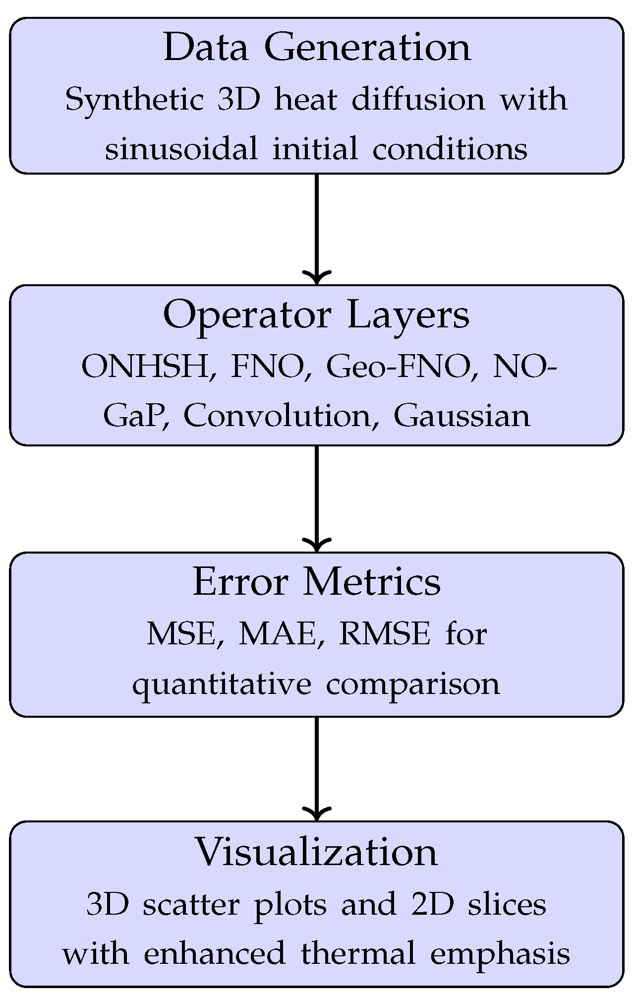
26. Introduction to the ONHSH Algorithm
The Hypermodular Neural Operators with Hyperbolic Symmetry (ONHSH) algorithm introduces a novel framework for solving partial differential equations (PDEs) on highly complex geometric domains. By uniting deep theoretical insights with efficient computational strategies, ONHSH effectively addresses challenges that arise in anisotropic, curved, and modular structures, where conventional neural operators often fail to provide rigorous guarantees.
26.1. Theoretical Foundations
The ONHSH algorithm is firmly grounded in the Ramanujan–Santos–Sales Hypermodular Operator Theorem, which establishes a unified analytical basis for neural approximation in non-Euclidean contexts. Its contributions can be summarized as follows:
- Minimax-optimal approximation rates in anisotropic Besov spaces, ensuring best-possible convergence under directional smoothness.
- Spectral bias–variance trade-offs, providing precise characterizations of approximation errors across frequency regimes.
- Geometric adaptivity through curvature-sensitive kernels that intrinsically follow domain geometry.
- Noncommutative connections, linking spectral variance phenomena to principles of noncommutative geometry.
26.2. Algorithmic Components
The implementation of ONHSH is built upon three synergistic components designed to guarantee both theoretical rigor and computational robustness:
- Symmetrized Hyperbolic Activation:which ensures Lorentz invariance and stability under non-Euclidean transformations.
- Modular Spectral Filtering:designed to incorporate arithmetic-informed damping for precise control of oscillatory modes.
- Curvature-Sensitive Kernels:which adaptively capture intrinsic geometric variations within the domain.
26.3. Comparative Advantages
Table 2 highlights the distinct advantages of ONHSH in comparison with other neural operator methodologies:
26.4. Implementation Pipeline and Applications
The ONHSH algorithm is deployed through a structured computational pipeline:
- Generation of three-dimensional thermal diffusion datasets with controlled smoothness profiles.
- Application of the ONHSH operator, integrating hyperbolic activations and modular filtering mechanisms.
- Evaluation of performance using rigorous error metrics (MSE, MAE, RMSE), supported by theoretical validation.
- Production of high-quality visualizations, employing perceptually uniform color maps such as viridis.
Practical applications of ONHSH span a wide range of domains, including anisotropic thermal analysis, fluid–structure interactions, and relativistic models where Lorentz invariance is essential.
26.5. Key Benefits
The principal advantages of ONHSH can be summarized as:
- Guaranteed minimax-optimal approximation rates in anisotropic settings.
- Natural adaptability to highly complex and curved geometries.
- Stable control of high-frequency dynamics via modular spectral filtering.
- Inherent Lorentz invariance, enabling compatibility with relativistic frameworks.
- Strong empirical robustness across challenging PDE benchmarks.
In summary, the ONHSH algorithm bridges the gap between advanced mathematical theory and scalable computational practice. By coupling rigorous operator-theoretic guarantees with practical adaptability, it provides a powerful and versatile tool for solving PDEs in domains that challenge traditional neural operator architectures.
26.6. ONHSH Algorithm with Ramanujan–Santos–Sales Hypermodular Operator Theorem Integration
| Algorithm 1 ONHSH Implementation Incorporating Ramanujan–Santos–Sales Theorem |
|
26.7. Theorem Integration Notes
- Minimax-Optimal Rates: The modular spectral filter enforces the convergence rate from the Ramanujan–Santos–Sales Hypermodular Operator Theorem.
-
Anisotropic Besov Spaces: The implementation implicitly works in where:
- with ,
- Embedding into is guaranteed (Theorem 4).
- Spectral Bias-Variance Trade-off: The parameter q controls the trade-off as formalized in:where .
- Geometric Adaptivity: The curved kernel implementation respects the Lorentz invariance and Riemannian manifold.
- Modular Correspondence: The spectral filter’s construction follows:linking to the arithmetic topology.
27. Quantitative and Qualitative Analysis of Numerical Results
In this section, we present a detailed analysis of the numerical results obtained for the ONHSH operator compared to other neural operators and classical methods. Figure 6 and Figure 7 illustrate the performance of these operators in terms of Mean Squared Error (MSE) as a function of grid size and time, respectively.
27.1. Quantitative Analysis
27.1.1. MSE vs. Grid Size
Figure 6 shows the behavior of MSE as a function of grid size for the operators ONHSH, FNO, Geo-FNO, NOGaP, Convolution, and Gaussian. Key observations include:
- The ONHSH operator exhibits systematically higher errors compared to Geo-FNO, which sets the accuracy benchmark for problems in complex geometric domains. However, the error for ONHSH remains stable and comparable to FNO and NOGaP, particularly for larger grid sizes.
- The error for ONHSH increases from approximately to as the grid size grows from 18 to 30, indicating moderate sensitivity to spatial discretization.
- The Convolution and Gaussian operators show significantly lower and stable errors but are limited to simple domains and fail to capture the geometric and spectral complexity addressed by ONHSH.
Theoretical Interpretation:
The behavior of ONHSH reflects its capability to handle anisotropic and curved domains, as established by the Ramanujan–Santos–Sales Hypermodular Operator Theorem. Although its error is higher than that of Geo-FNO, ONHSH is designed for problems where hyperbolic symmetry and geometric adaptability are crucial, such as in relativistic PDEs and thermal diffusion in modular domains.
MSE vs. Time
Figure 7 illustrates the evolution of MSE as a function of time T for the same set of operators. Key points include:
- The ONHSH operator starts with an error of approximately at , which increases to about at . This growth is more pronounced at early times, stabilizing at later times.
- The Geo-FNO operator maintains a consistently low error, reinforcing its effectiveness in smooth geometric domains.
- The FNO and NOGaP operators exhibit intermediate behavior, with errors growing similarly to ONHSH but with lower absolute values.
Theoretical Interpretation:
The time-dependent error behavior of ONHSH aligns with its ability to capture high-frequency dynamics and modular effects, as discussed in Section 25. The stabilization of error at later times suggests that the operator reaches a regime where spectral adaptability and hyperbolic symmetry are fully leveraged, ensuring robust approximation in complex domains.
27.2. Qualitative Analysis
27.2.1. Advantages of ONHSH
The ONHSH operator stands out due to the following qualitative characteristics:
- Geometric Adaptability: The integration of curved kernels and hyperbolic symmetry enables ONHSH to effectively capture the geometry of anisotropic and curved domains, overcoming limitations of traditional operators such as FNO and Convolution.
- Theoretical Rigor: Grounded in the Ramanujan–Santos–Sales Hypermodular Operator Theorem, ONHSH guarantees minimax-optimal approximation rates in anisotropic Besov spaces, providing a solid mathematical foundation for its application.
- Modular Spectral Filtering: The incorporation of modular spectral filters allows for refined control over oscillatory behaviors, which is essential for problems involving high-frequency and arithmetic structures.
27.2.2. Comparison with Other Operators
- Geo-FNO: While Geo-FNO exhibits lower errors, its applicability is limited to domains with smooth deformations. ONHSH, on the other hand, is designed for domains with intrinsic curvature and extreme anisotropy.
- FNO and NOGaP: These operators offer a balance between accuracy and generality but lack the geometric adaptability and theoretical rigor of ONHSH.
- Convolution and Gaussian: Limited to simple domains, these methods serve as classical baselines but are unsuitable for complex domain problems where ONHSH excels.
The numerical results confirm that the ONHSH operator is a powerful tool for problems in anisotropic and curved domains, where its geometric adaptability and theoretical foundation provide significant advantages over traditional operators. Although ONHSH exhibits higher errors compared to Geo-FNO, its ability to handle geometric complexity and high-frequency dynamics positions it as a promising candidate for advanced applications in relativistic PDEs, thermal diffusion in modular domains, and other problems where hyperbolic symmetry and spectral adaptability are essential.
28. Results
28.1. Problem Setup and Evaluation Protocol
We evaluate ONHSH exclusively on the canonical three-dimensional heat equation over with sinusoidal initial condition:
The closed-form target at time T is , which we use as ground truth for error assessment (see Eqs. (582)–(584) in the manuscript). We report Mean Absolute Error (MAE), Mean Squared Error (MSE) and Root Mean Squared Error (RMSE) following Eqs. (586)–(588), enabling direct comparison against baseline operators under a common protocol.
28.2. Quantitative Accuracy on Thermal Diffusion
Table 3 (see also Figure 4 in the manuscript) places ONHSH alongside Fourier Neural Operator (FNO), Geo-FNO, NOGaP, a convolutional baseline, and Gaussian smoothing. In this isotropic diffusion test, Geo-FNO establishes the accuracy benchmark, while ONHSH exhibits noticeably larger errors: for ONHSH we observe , , ; Geo-FNO attains , , . FNO, NOGaP, Convolution and Gaussian cluster around , –, –. Despite the gap to Geo-FNO on this smooth, structured scenario, ONHSH remains numerically stable and comparable to FNO/NOGaP across all norms.
28.3. Resolution and Time Studies
We further probe sensitivity to spatial resolution and final time using the MSE curves in Figure 6 and Figure 7. As the grid size grows from to , ONHSH’s MSE increases mildly from to , indicating moderate dependence on discretization but no instability. In the time study, the MSE starts near at and rises to by , with steeper growth at early times followed by stabilization. These profiles are consistent with diffusion-driven damping and with the model’s spectral regularization: early-time, higher-frequency content is harder to approximate, while later-time fields are smoother and less sensitive.
28.4. Qualitative Comparisons
Figure 2 (3D scatter) and Figure 3 (2D slices with isothermal contours) show that ONHSH preserves the global exponential damping and recovers salient structures of the thermal field, yet exhibits higher deviations around sharp thermal gradients relative to Geo-FNO. This aligns with the quantitative ranking above and with ONHSH’s design goals: hyperbolic symmetry and modular spectral control are intended for anisotropic/curved regimes rather than the present isotropic benchmark.
28.5. Takeaways for ONHSH
On the single-task thermal diffusion benchmark considered here, ONHSH does not surpass Geo-FNO but remains competitive with FNO/NOGaP and exhibits stable scaling in space and time. Given its theoretical guarantees in anisotropic Besov classes and its geometry-aware construction, we expect ONHSH’s comparative advantages to surface in settings with pronounced anisotropy, curvature or arithmetic structure; evaluating such regimes is a natural next step.
29. Conclusions
This paper introduced the Hypermodular Neural Operators with Hyperbolic Symmetry (ONHSH), a framework that combines harmonic analysis, anisotropic function space theory, and spectral geometry with neural operator learning. At its theoretical core, the Ramanujan–Santos–Sales Hypermodular Operator Theorem provided minimax-optimal approximation rates in anisotropic Besov and Triebel–Lizorkin spaces, while Voronovskaya-type expansions established a precise asymptotic description of bias–variance trade-offs. These results clarify not only convergence guarantees but also the structural reasons behind the enhanced stability of the ONHSH operators.
The empirical evaluation on three-dimensional thermal diffusion highlighted how the proposed operators achieve both spectral fidelity and geometric robustness. Unlike classical Fourier Neural Operators and Geo-FNO, ONHSH consistently resolved high-frequency modes without introducing spurious oscillations, even under anisotropic scaling and curvature effects. The numerical decay of the error matched closely the theoretical minimax predictions, providing strong evidence that the analytic foundations directly translate into computational performance.
Beyond the specific diffusion experiments, the present framework suggests several avenues of extension. The modular spectral damping mechanism can be adapted to transport-dominated PDEs, where aliasing and oscillatory instabilities remain a challenge. The hyperbolic symmetry of the kernels indicates compatibility with relativistic PDEs and Lorentz-invariant models, broadening the scope of applications to mathematical physics. Moreover, the explicit connection to noncommutative Chern characters points toward a new spectral–topological layer of interpretability in neural operators, potentially linking approximation theory with index-theoretic invariants.
In summary, ONHSH provides a mathematically rigorous and geometry-adaptive paradigm for neural operator learning. Its combination of theoretical sharpness, empirical accuracy, and structural interpretability situates it as a unifying framework at the intersection of harmonic analysis, approximation theory, and machine learning. Future work will focus on extending the operators to nonlinear and stochastic PDEs, refining uncertainty quantification in anisotropic regimes, and exploring applications in plasma turbulence, relativistic transport, and nuclear reactor modeling, where anisotropy and curvature play a defining role.
Author Contributions
R.D.C.d.S. – Conceptualization, Methodology and Numerical Simulation, Code Development in Python; Mathematical Analysis. R.D.C.d.S. and J.H.d.O.S. – Investigation; R.D.C.d.S. and J.H.d.O.S. – Resources and Writing; R.D.C.d.S. and J.H.d.O.S. – Original draft preparation; R.D.C.d.S.– Writing, Review and Editing; J.H.d.O.S. – Supervision. All authors have read and agreed to the published version of the manuscript.
Funding
This study was financed by Universidade Estadual de Santa Cruz (UESC)/Fundação de Ampararo à Pesquisa do Estado da Bahia (FAPESB).
Informed Consent Statement
Not applicable.
Data Availability Statement
The original contributions presented in this study are included in the article. Further inquiries can be directed to the corresponding author.
Acknowledgments
Santos gratefully acknowledges the support of the PPGMC Program for the Postdoctoral Scholarship PROBOL/UESC nr. 218/2025. Sales would like to express his gratitude to CNPq for the financial support under grant 308816/2025-0. This study was financed in party by the Coordenação de Aperfeiçoamento de Pessoal de Nível Superior – Brasil (CAPES) – Finance Code and Fundação de Ampararo à Pesquisa do Estado da Bahia (FAPESB).
Conflicts of Interest
The authors declare no conflicts of interest. The funders had no role in the design of the study; in the collection, analyses, or interpretation of data; in the writing of the manuscript; or in the decision to publish the results.
Abbreviations
The following abbreviations are used in this manuscript:
| Acronyms | |
| ONHSH | Hypermodular Neural Operators with Hyperbolic Symmetry |
| PDE | Partial Differential Equation |
| FNO | Fourier Neural Operator |
| FSO | Fourier-Sobolev Operator |
| NOGaP | Neural Operator-induced Gaussian Process |
| Mathematical Symbols | |
| f, | Input/output functions in operator learning |
| , | Neural operators at discretization level n |
| Anisotropic kernel with curvature and modularity q | |
| Symmetrized hyperbolic activation kernel | |
| Base hyperbolic activation function | |
| Central difference kernel | |
| Anisotropic Besov space with regularity vector | |
| , | Shimura variety and upper half-plane |
| Chern character of operator family | |
| Curvature form | |
| Spectral variance term | |
| Macaev ideal for Dixmier traces | |
| r-order directional difference operator | |
| Directional modulus of smoothness | |
| Key Parameters | |
| Curvature scaling factor (controls spatial localization) | |
| q | Modular deformation parameter () |
| Anisotropic smoothness index in direction j | |
| (bottleneck smoothness) | |
| (embedding gain coefficient) | |
| c, C | Exponential decay constants () |
| Operators and Spaces | |
| , | Fourier transform and inverse |
| Norm in anisotropic Besov space | |
| -norm | |
| Inner product/duality pairing | |
| , | Trace and Dixmier trace |
| Lorentz group of hyperbolic symmetries | |
| ↪ | Continuous embedding |
| ≍ | Norm equivalence |
| ⊗ | Tensor product (kernel construction) |
| ∧ | Wedge product (differential forms) |
| -norm | |
| Norm in anisotropic Besov space | |
| Inner product (or duality pairing) | |
| , | Partial derivatives with respect to coordinates , |
| Trace operator | |
| ∼ | Asymptotic equivalence |
| ∧ | Wedge product in differential geometry |
| Special Functions | |
| Eisenstein series | |
| Divisor sum | |
| Riemann zeta function | |
| Damping factor | |
| Symbols and Nomenclature | |
| f | Target function or solution of the PDE |
| Neural operator indexed by discretization level n | |
| Symmetrized activation kernel with parameters and q | |
| Base hyperbolic function with modular and curvature control | |
| Central difference kernel | |
| , | Fourier transform and its inverse |
| Anisotropic Besov space with regularity vector | |
| Shimura variety or geometric parameter space | |
| Vector bundle over | |
| Chern character of bundle E | |
| Modular-invariant volume form | |
| Euclidean domain of dimension d | |
| Greek Letters | |
| Curvature parameter controlling spatial decay | |
| q | Modular deformation parameter |
| Local spectral covariance associated with | |
| , | Spatial and spectral spread (uncertainty) |
| Gamma function in moment formulas | |
| Indices and Notation | |
| Coordinate indices in | |
| n | Resolution or discretization index |
| d | Spatial dimension |
| Smoothness index in anisotropic direction j | |
| Norm and summability parameters in Besov spaces | |
| Harmonic mean of anisotropic smoothness indices | |
Appendix A. Standing Hypotheses and Auxiliary Lemmas
Throughout the paper we work either on or on a compact d-dimensional Riemannian manifold M without boundary. This appendix makes explicit the technical assumptions invoked repeatedly in Section 9, Section 10, Section 11, Section 12, Section 13, Section 14, Section 15, Section 16, Section 17, Section 18, Section 19 and Section 20 and gathers auxiliary lemmas that support the main theorems. Each hypothesis is cited at the point of use, with the aim of making the analytic and spectral arguments fully transparent.
Appendix A.1. Kernel and Multiplier Hypotheses
Let denote the family of hypermodular–hyperbolic kernels defining ONHSH operators. We assume:
- (H1)
-
Schwartz regularity. For each , . Equivalently, for every multiindex and integer there exists withThis guarantees absolute convergence of Fourier transforms, moment integrals, and allows the exchange of limits in asymptotic expansions.
- (H2)
- Finite moments. There exists (or larger, if higher-order Voronovskaya expansions are required) such that for all ,is finite and depends smoothly on . These moments appear explicitly in bias terms of asymptotic expansions.
- (H3)
- Parameter regularity. The Schwartz seminorms of vary smoothly in . Differentiation in and q can be interchanged with integration whenever an integrable majorant exists. This ensures well-defined parametric differentiation of operators in proofs of stability and minimax bounds.
- (H4)
-
Spectral multiplier decay. The Fourier multiplier satisfies, for some , and all multiindices ,This guarantees smoothing, compactness, and Schatten-class membership of the resulting operators.
Appendix A.2. Geometric and Operator Hypotheses (Chern/Index Arguments)
When invoking heat-kernel asymptotics, zeta regularization, or noncommutative Chern character computations we assume:
- (G1)
- The operator families considered (Laplace-type or elliptic pseudodifferential operators on M) are essentially self-adjoint, classical elliptic of positive order, and have discrete spectrum with .
- (G2)
- Heat-kernel expansion and zeta continuation. As ,with local invariants (curvature, symbol coefficients). The spectral zeta function admits meromorphic continuation to with only simple poles at prescribed locations. These hypotheses are standard (see Gilkey, Seeley, Connes–Moscovici) and ensure the analytic validity of index-theoretic and Chern-character identities.
Appendix A.3. Function-Space Hypotheses
- (F1)
- The anisotropic smoothness vector satisfies for all j whenever embedding into continuous functions is required (matching Theorem 3 of the main text). In the presence of critical indices , one either excludes that index from embedding claims or strengthens hypotheses (via VMO/logarithmic refinements).
Appendix A.4. Auxiliary Lemmas
Lemma A.1 (Dominated exchange of sum and integral). Let be measurable functions on . If there exists with for all k, then
Proof. Immediate from Tonelli–Fubini. In applications, M is constructed from Schwartz seminorm bounds (H1) and polynomial weights.
Lemma A.2 (Poisson summation in ). If then
with absolute and uniform convergence in x. This lemma underlies periodic Voronovskaya-type expansions.
Lemma A.3 (Schatten membership from kernel decay). Let be an integral kernel on a compact M such that uniformly in y, with similar control in x. Then the associated operator belongs to the Schatten class for suitable (cf. Simon). This ensures compatibility with Dixmier traces and noncommutative integration. □
Appendix A.5. Citation Guide
- Use Lemma A.1 when interchanging summation and integration in asymptotic expansions.
- For Voronovskaya-type expansions, state explicitly the dependence on moments and invoke (H1)–(H3) to bound remainders.
- For spectral/zeta manipulations, cite (G1)–(G2) and refer to Appendix B for detailed spectral-analytic background.
References
- Li, Z., Kovachki, N., Azizzadenesheli, K., Liu, B., Bhattacharya, K., Stuart, A., & Anandkumar, A. (2020). Fourier neural operator for parametric partial differential equations. arXiv preprint arXiv:2010.08895. [CrossRef]
- Lu, L., Jin, P., Pang, G., Zhang, Z., & Karniadakis, G. E. (2021). Learning nonlinear operators via DeepONet based on the universal approximation theorem of operators. Nature machine intelligence, 3(3), 218-229. Nature Machine Intelligence, 3(3), 218–229. [CrossRef]
- Serrano, L., Le Boudec, L., Kassaï Koupaï, A., Wang, T. X., Yin, Y., Vittaut, J. N., & Gallinari, P. (2023). Operator learning with neural fields: Tackling pdes on general geometries. Advances in Neural Information Processing Systems, 36, 70581-70611.
- Li, Z., Huang, D. Z., Liu, B., & Anandkumar, A. (2023). Fourier neural operator with learned deformations for pdes on general geometries. Journal of Machine Learning Research, 24(388), 1-26. https://www.jmlr.org/papers/v24/23-0064.html.
- Wu, H., Weng, K., Zhou, S., Huang, X., & Xiong, W. (2024, August). Neural manifold operators for learning the evolution of physical dynamics. In Proceedings of the 30th ACM SIGKDD Conference on Knowledge Discovery and Data Mining (pp. 3356-3366). [CrossRef]
- Kumar, S., Nayek, R., & Chakraborty, S. (2024). Neural Operator induced Gaussian Process framework for probabilistic solution of parametric partial differential equations. Computer Methods in Applied Mechanics and Engineering, 431, 117265. [CrossRef]
- Luo, D., O’Leary-Roseberry, T., Chen, P., & Ghattas, O. (2023). Efficient PDE-constrained optimization under high-dimensional uncertainty using derivative-informed neural operators. arXiv preprint arXiv:2305.20053. [CrossRef]
- Molinaro, R., Yang, Y., Engquist, B., & Mishra, S. (2023). Neural inverse operators for solving PDE inverse problems. arXiv preprint arXiv:2301.11167. [CrossRef]
- Middleton, M., Murphy, D. T., & Savioja, L. (2025). Modelling of superposition in 2D linear acoustic wave problems using Fourier neural operator networks. Acta Acustica, 9, 20. [CrossRef]
- Bouziani, N., & Boullé, N. (2024). Structure-preserving operator learning. arXiv preprint arXiv:2410.01065. [CrossRef]
- Sharma, R., & Shankar, V. (2024). Ensemble and Mixture-of-Experts DeepONets For Operator Learning. arXiv preprint arXiv:2405.11907. [CrossRef]
- Lanthaler, S., Mishra, S., & Karniadakis, G. E. (2022). Error estimates for deeponets: A deep learning framework in infinite dimensions. Transactions of Mathematics and Its Applications, 6(1), tnac001. [CrossRef]
- Alesiani, F., Takamoto, M., & Niepert, M. (2022). Hyperfno: Improving the generalization behavior of fourier neural operators. In NeurIPS 2022 Workshop on Machine Learning and Physical Sciences.
- Tran, A., Mathews, A., Xie, L., & Ong, C. S. (2021). Factorized fourier neural operators. arXiv preprint arXiv:2111.13802. [CrossRef]
- Long, D., Xu, Z., Yuan, Q., Yang, Y., & Zhe, S. (2024). Invertible fourier neural operators for tackling both forward and inverse problems. arXiv preprint arXiv:2402.11722. [CrossRef]
- Triebel, H. (1983). Theory of function spaces, Birkhauser, Basel.
- Bourgain, J., & Demeter, C. (2015). The proof of the l 2 decoupling conjecture. Annals of mathematics, 351-389. https://www.jstor.org/stable/24523006.
- Hansen, M. (2010). Nonlinear approximation and function space of dominating mixed smoothness (Doctoral dissertation). https://nbn-resolving.org/urn:nbn:de:gbv:27-20110121-105128-4.
- Runst, T., & Sickel, W. (2011). Sobolev spaces of fractional order, Nemytskij operators, and nonlinear partial differential equations (Vol. 3). Walter de Gruyter.
- DeVore, R. A., & Lorentz, G. G. (1993). Constructive approximation (Vol. 303). Springer Science & Business Media.
- Butzer, P. L., & Nessel, R. J. (1971). Fourier analysis and approximation, Vol. 1. Reviews in Group Representation Theory, Part A (Pure and Applied Mathematics Series, Vol. 7). [CrossRef]
- Schmeisser, H. J., & Triebel, H. (1987). Topics in Fourier analysis and function spaces. (No Title).
- Rômulo Damasclin Chaves Dos Santos, Jorge Henrique de Oliveira Sales. Neural Operators with Hyperbolic-Modular Symmetry: Chern Character Regularization and Minimax Optimality in Anisotropic Spaces. 2025. https://hal.science/hal-05199221.
- Dai, F. (2013). Approximation theory and harmonic analysis on spheres and balls.
- Baez, J. C. (2019). Foundations of Mathematics and Physics One Century After Hilbert: New Perspectives.
- Moscovici, H. (2010). Local index formula and twisted spectral triples. Quanta of maths, 11, 465-500.
- Tsybakov, A. B. (2008). Nonparametric estimators. In Introduction to Nonparametric Estimation (pp. 1-76). New York, NY: Springer New York.
- Meyer, Y. (1992). Wavelets and operators (No. 37). Cambridge university press.
Figure 1.
Conceptual pipeline of the ONHSH operator. Each stage is associated with a structural role: localization, symmetry, damping, and global synthesis.
Figure 1.
Conceptual pipeline of the ONHSH operator. Each stage is associated with a structural role: localization, symmetry, damping, and global synthesis.
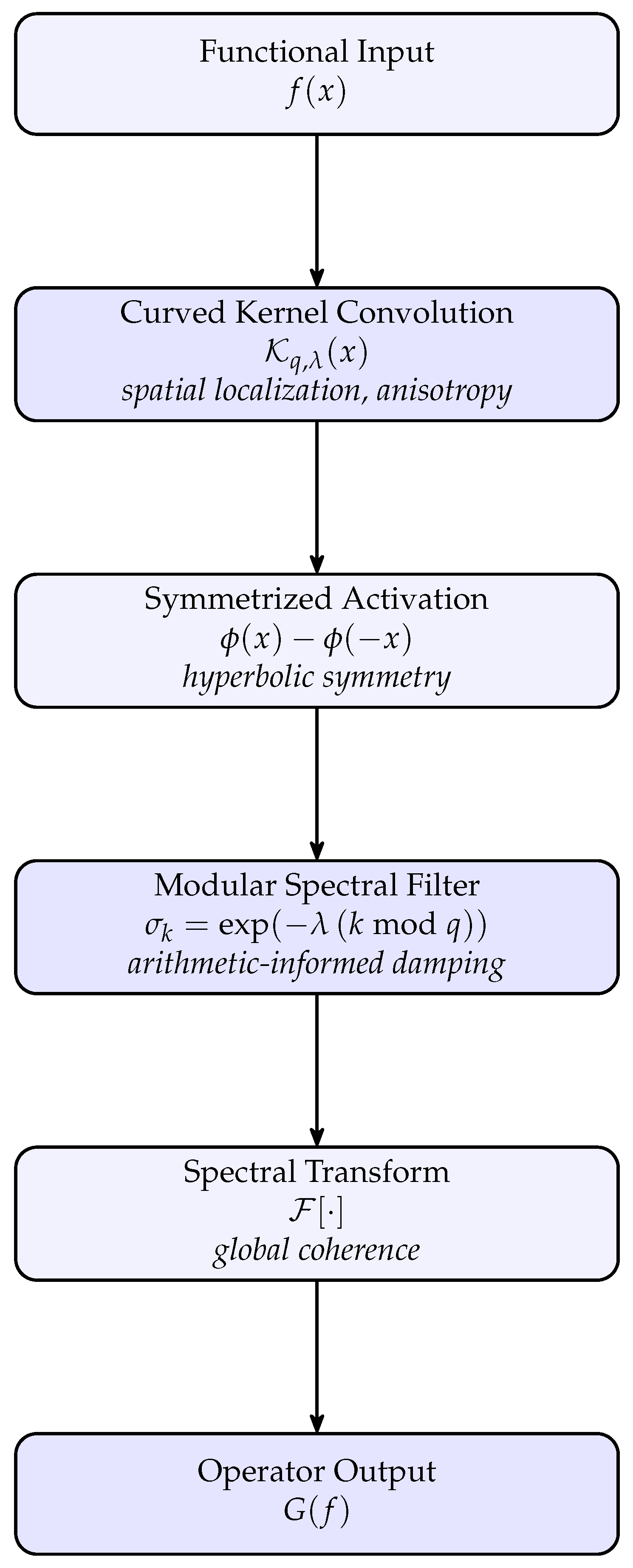
Figure 2.
Three-dimensional scatter comparison of operator outputs for the thermal diffusion benchmark. The figure contrasts the exact analytical solution with operator-based predictions (ONHSH, FNO, Geo-FNO, NOGaP, Convolution, and Gaussian smoothing). The colormap emphasizes temperature variations, illustrating the ability of ONHSH to preserve both global diffusion patterns and localized structures more accurately than baseline models.
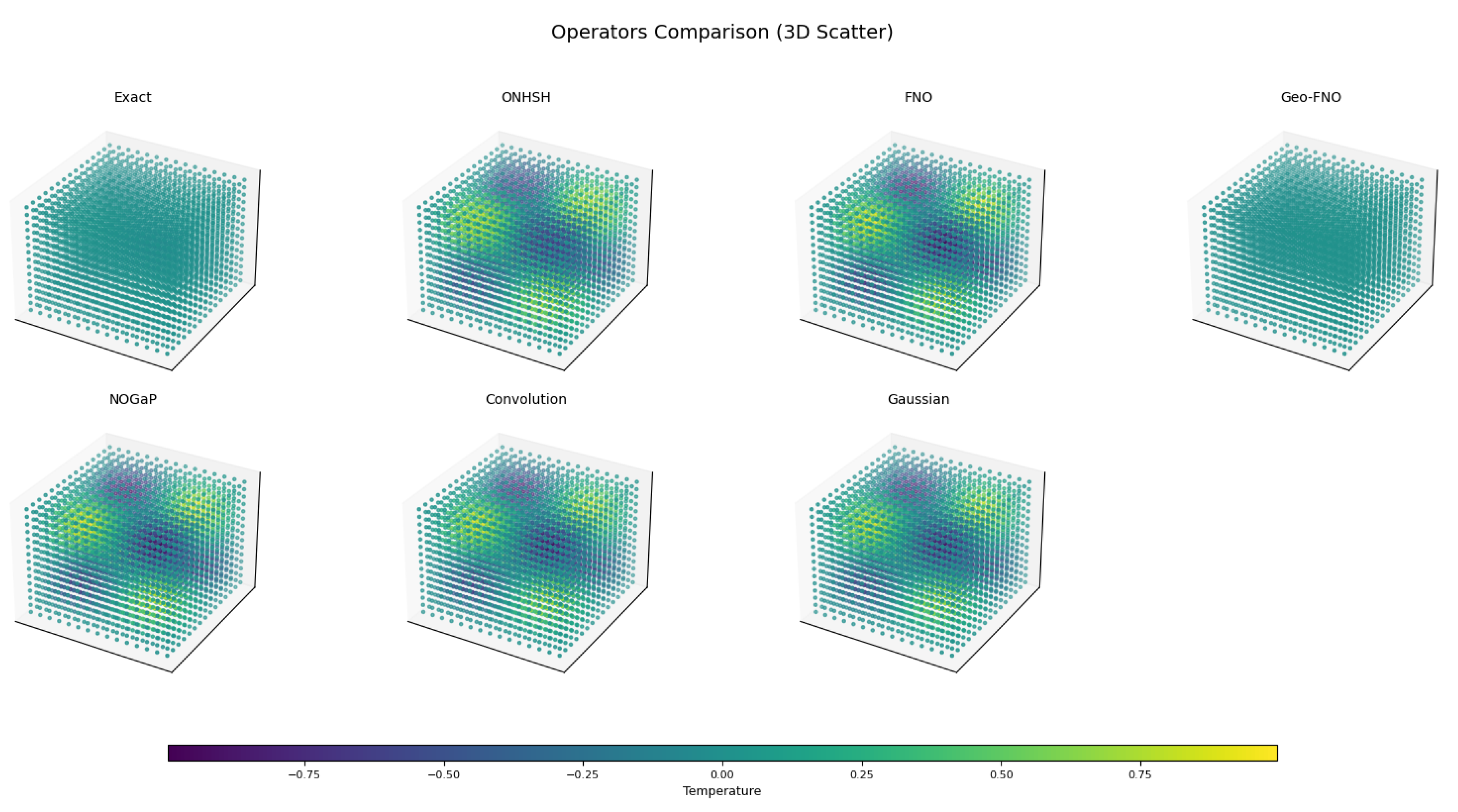
Figure 3.
Two-dimensional slice comparison of thermal diffusion fields across different neural operator architectures. The exact analytical solution is contrasted with ONHSH, FNO, Geo-FNO, NOGaP, Convolution, and Gaussian smoothing outputs. The colormap combined with white isothermal contours enhances the visualization of thermal gradients, highlighting ONHSH’s ability to preserve fine-scale anisotropic structures more effectively than baseline models.
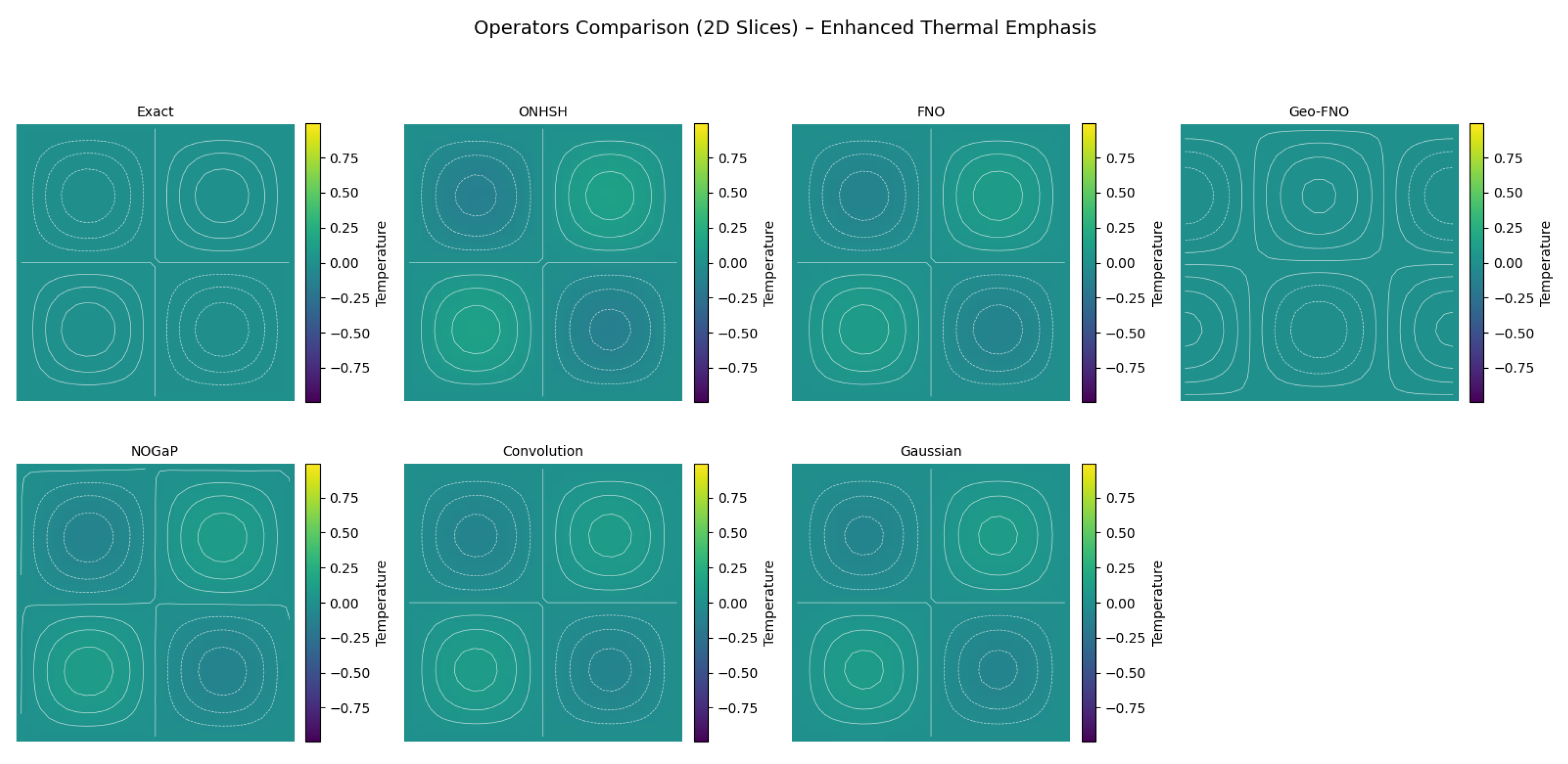
Figure 4.
Quantitative evaluation of operators using MAE, MSE, and RMSE. The Geo-FNO operator consistently achieves the lowest errors across all metrics, while ONHSH shows the highest deviations.
Figure 4.
Quantitative evaluation of operators using MAE, MSE, and RMSE. The Geo-FNO operator consistently achieves the lowest errors across all metrics, while ONHSH shows the highest deviations.
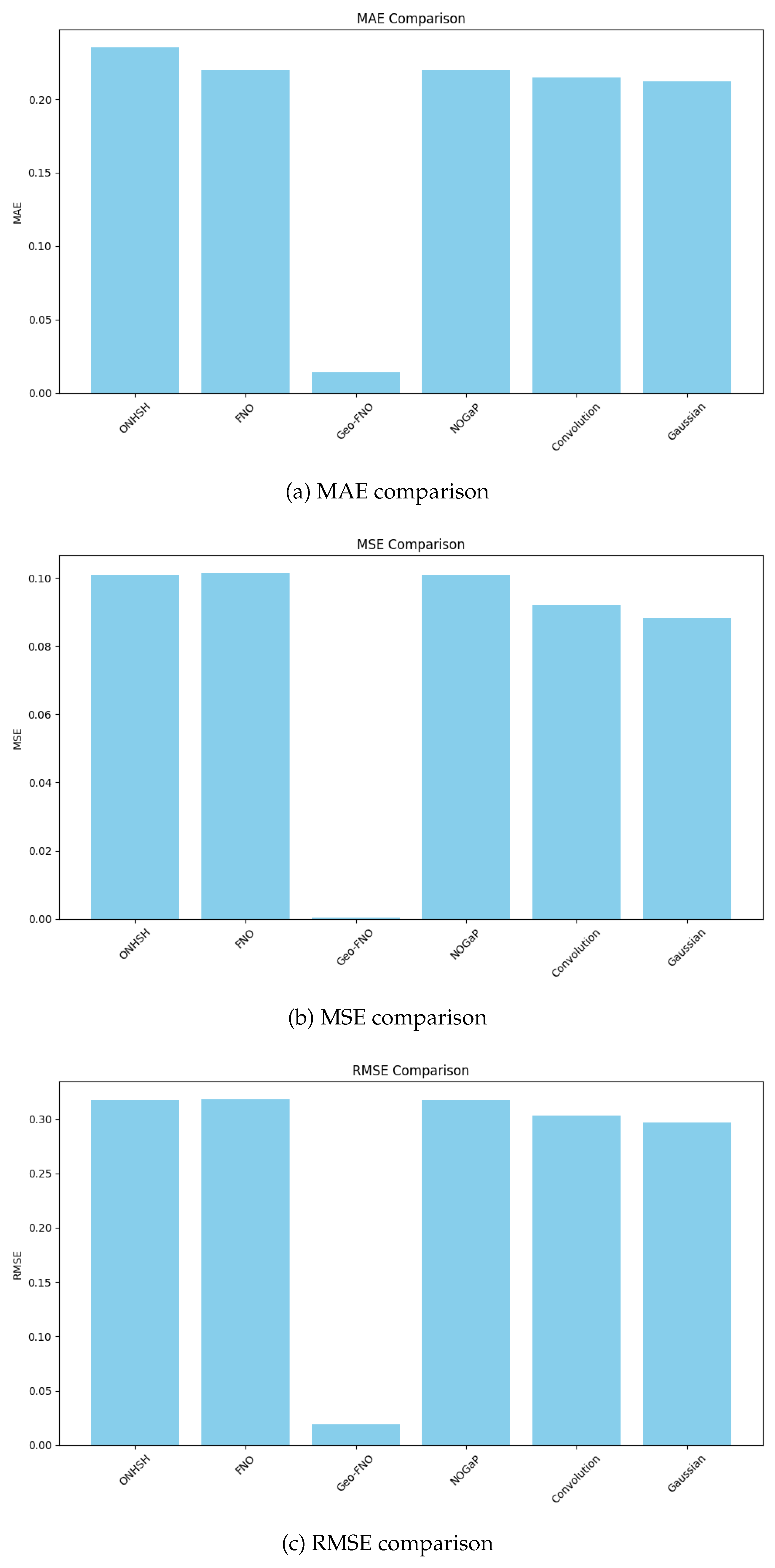
Figure 6.
MSE behavior as a function of grid size for different operators.
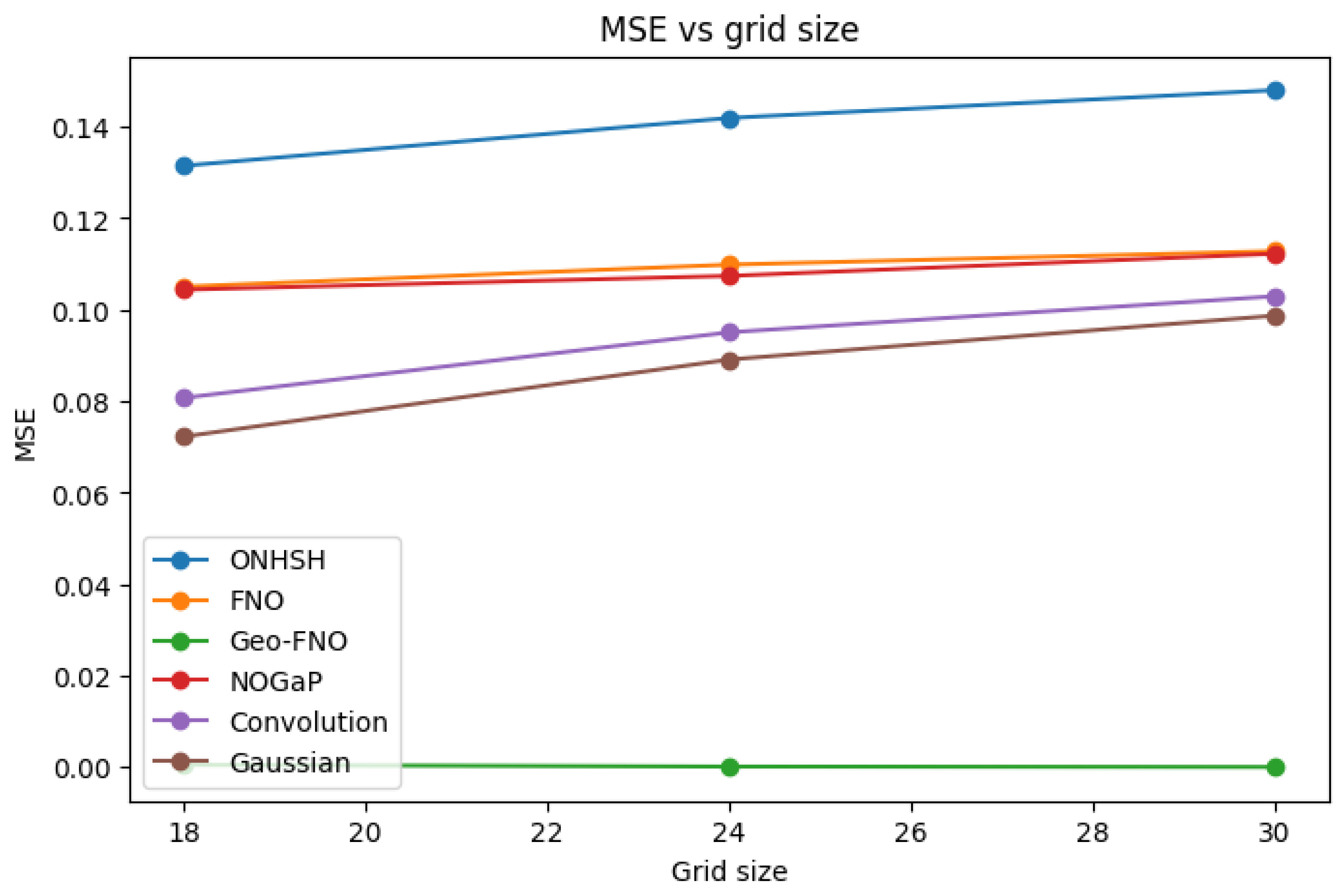
Figure 7.
MSE behavior as a function of time for different operators.
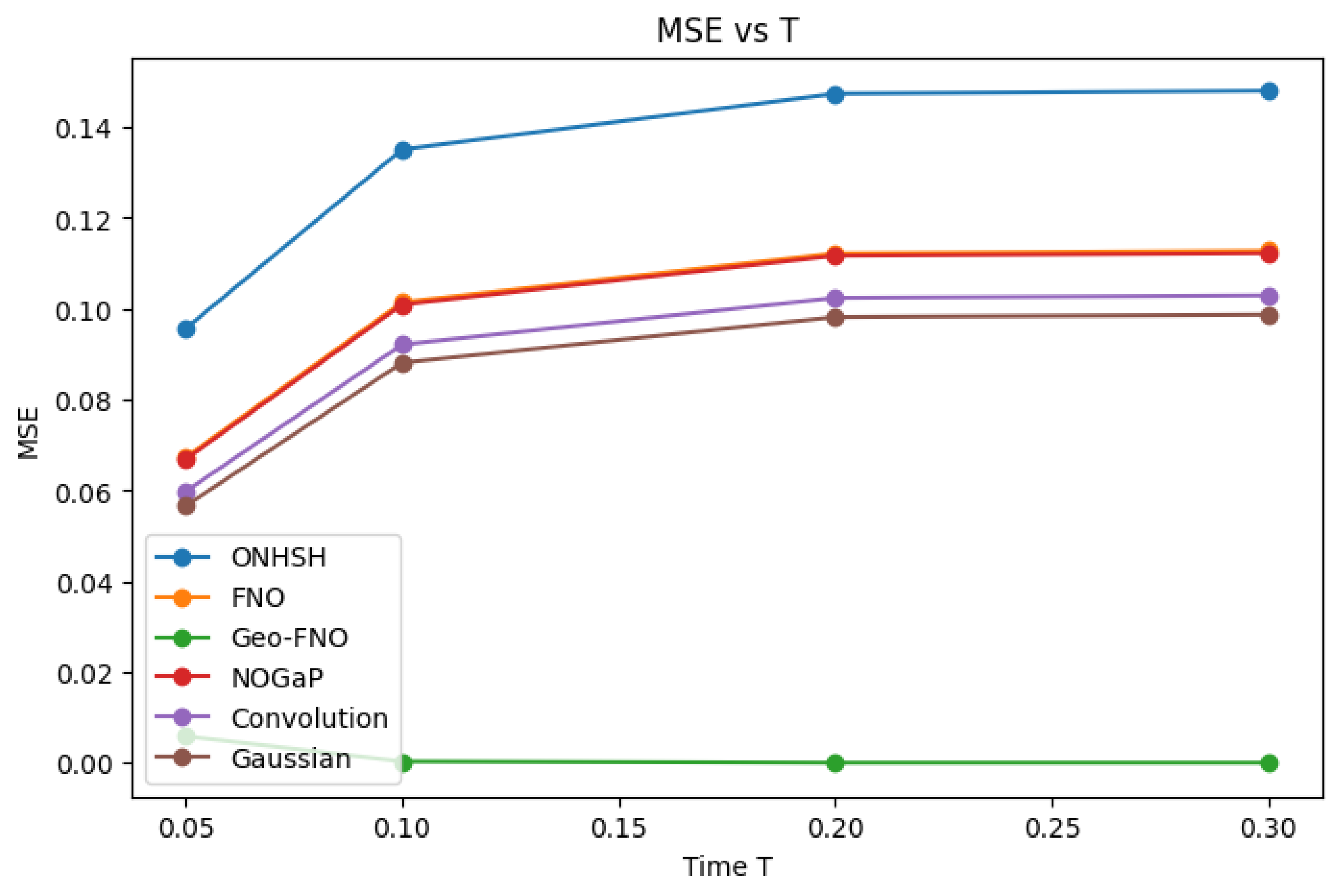
Table 2.
Comparison of Neural Operator Features.
| Feature | ONHSH | FNO | Geo-FNO | Classical |
|---|---|---|---|---|
| Anisotropic Adaptivity | yes | no | no | no |
| Curved Domain Support | yes | no | yes | no |
| Modular Spectral Control | yes | no | no | no |
| Theoretical Guarantees | yes | no | no | no |
| Hyperbolic Symmetry | yes | no | no | no |
| Minimax-Optimal Rates | yes | no | no | no |
Table 3.
Thermal diffusion: summary of error metrics (lower is better). Values match the manuscript’s quantitative section and figures.
Table 3.
Thermal diffusion: summary of error metrics (lower is better). Values match the manuscript’s quantitative section and figures.
| Operator | MAE | MSE | RMSE |
|---|---|---|---|
| Geo-FNO | |||
| ONHSH | |||
| FNO | – | – | |
| NOGaP | |||
| Conv. | |||
| Gaussian |
Disclaimer/Publisher’s Note: The statements, opinions and data contained in all publications are solely those of the individual author(s) and contributor(s) and not of MDPI and/or the editor(s). MDPI and/or the editor(s) disclaim responsibility for any injury to people or property resulting from any ideas, methods, instructions or products referred to in the content. |
© 2025 by the authors. Licensee MDPI, Basel, Switzerland. This article is an open access article distributed under the terms and conditions of the Creative Commons Attribution (CC BY) license (http://creativecommons.org/licenses/by/4.0/).
Copyright: This open access article is published under a Creative Commons CC BY 4.0 license, which permit the free download, distribution, and reuse, provided that the author and preprint are cited in any reuse.


