
Submitted:
19 September 2025
Posted:
19 September 2025
You are already at the latest version
Abstract
This paper presents two fundamental principles redefining reality: electromagnetic phenomena are two-dimensional and follow the Cauchy distribution; and there exists a non-integer variable dimensionality of spaces. These principles explain massless electromagnetic fields and their interaction with matter. Four specific, cost-effective zones of verification and falsification are presented, all accessible with standard laboratory equipment: (1) a reverse slit experiment examining the shadow from a thin object; (2) optimization of single-mode optical fiber transmission; (3) enhancement of astronomical images through Cauchy kernel processing; and (4) modification of satellite communication systems and antenna designs. The central question: does light propagation follow the Cauchy distribution (compatible with exact two-dimensionality D=2.0 of massless electromagnetic fields) rather than the traditionally expected sinc$^2$ function. The proposed concept of variable dimensionality explains the nature of mass as a dimensional effect arising only when deviating from the critical point D=2.0, offers a new interpretation of the relationship $E=mc^2$, and reveals the deep meaning of time through information asymmetry and synchronization mechanisms. This framework resolves fundamental contradictions in modern physics and has revolutionary implications for quantum mechanics, relativity theory, and cosmology, potentially eliminating the need for concepts such as dark energy and inflationary cosmology. Further mathematical development demonstrates how the timeless Schr\"odinger equation emerges naturally as an optimization problem in Fourier space for systems with dimensionality D=2-$\epsilon$, providing a novel interpretation of quantum phenomena as projections between spaces of different dimensionality. Classical mechanics from Newton to Feynman emerges as spectral filtering in frequency space, while thermodynamic irreversibility dissolves into measurement-induced spectral folding rather than fundamental time asymmetry. The paper reveals rotation as a universal codec enabling dimensional synchronization through the 2D electromagnetic channel, with Fourier transformation serving as the fundamental mechanism. The uncertainty principle is merely Cauchy-Schwarz inequality in Fourier space, making $\hbar$/2 a mathematical necessity rather than cosmic mystery. The ultraviolet catastrophe is reinterpreted as a statistical error --- applying Gaussian assumptions to inherently Cauchy-distributed cavity modes --- with Planck's quantization emerging naturally from the Fourier --- Cauchy codec rather than requiring metaphysical discreteness. Kepler's laws arise from 2D electromagnetic channel constraints without gravitational forces. The framework connects to EPI principles, showing Cauchy distributions as informationally optimal at D=2. Empirical validation through analysis of 300,000 Hubble Space Telescope stellar observations across 20 sky regions reveals the unique signature predicted by Principle I: universal convergence to Moffat parameter $\alpha \approx 1.5$ without detectable dispersion, confirming the squared Cauchy distribution of electromagnetic intensity. Anyone can verify these fundamental principles at home using their smartphone photographs and immediately see visible improvement in image quality. Analysis of 3,000+ quasar spectra reveals frequency-dependent redshift deviations with perfect correlations, fundamentally challenging the Doppler interpretation and universal expansion hypothesis.
Keywords:
two-dimensional electromagnetic field
; cauchy distribution
; variable dimensionality of spaces
; hubble space telescope observations
; moffat profile analysis
; extreme physical information
; information geometry
; fourier space optimization
; information asymmetry
; photon masslessness
; nature of time
; fisher information matrix
; schrödinger equation
; dimensional flow
; empirical validation
; point spread function
; smartphone image enhancement
; home verification
; accessible experiments
; gaussian vs cauchy deconvolution
; image deconvolution
; mass emergence
; Lorentz invariance
; medical imaging applications
; real-time benefits
; cosmological redshift
; frequency-dependent redshift
; SDSS quasar analysis
; universal expansion challenge
; anisotropic redshift
; directional cosmology
; rotation as dimensional codec
; gnomonic projection
; bessel function decoding
; blackbody radiation
; dynamics
; thermodynamics
; spectral filtering
; maximum entropy method
; orbital mechanics
; wide sense stationary
0. Structure and Evolution of This Document
This manuscript represents an iterative development process. Previous versions are included in their entirety, with each successive version appending new sections to the appendices while preserving all earlier content unchanged. This additive methodology was adopted to maintain the logical consistency of the theoretical framework across iterations.
The resulting structure explains certain unconventional characteristics: appendices contain materials from different developmental stages, some concepts are approached from multiple perspectives, and analytical depth increases in later sections. This evolutionary approach documents the systematic emergence of the theoretical framework.
1. Introduction
Light, as a fundamental physical phenomenon, has been at the center of our understanding of the universe for more than three centuries. The nature of light has been constantly reinterpreted with each new revolution in physics, but a fundamental question remains open: is light a truly three-dimensional phenomenon, similar to other physical objects in our world, or is its nature fundamentally different?
Modern physics has established that the photon, the quantum of the electromagnetic field, has zero rest mass. Experimental constraints indicate an upper limit on the photon mass of kg, which is consistent with exact masslessness. However, the masslessness of the photon creates a profound contradiction with the assumption of three-dimensionality of light phenomena. A massless particle cannot have finite statistical moments of distribution — a fundamental mathematical requirement that is inconsistent with the Gaussian character of distribution expected for three-dimensional phenomena.
This contradiction points to the need to revise our basic concepts of the nature of light and space. This paper proposes a radically new view of these fundamental concepts, based on two principles that will be formulated in the next section.
For readers interested in the historical context of the development of ideas about light, space, and time, Appendix 1 presents a historical overview. It examines the contributions of key figures, including Hendrik and Ludwig Lorentz, Augustin-Louis Cauchy, Henri Poincaré, and Albert Einstein, in shaping modern views on electromagnetic phenomena and the dimensionality of space or space-time.
The evolution and historical background of the concept of time represents a separate extensive topic, which is partially addressed in the appendices, but it is important to mention now that, surprisingly, there is no unified theory of time, clocks, or measurements. The question is still unresolved, and there is no definition or consensus about what parameter is used for differentiating the Lagrangians that are at the heart of dynamics. The uncertainty of time manifests itself in other areas of physics as well.
To provide deeper insights into the implications of our proposed principles, the appendices include several thought experiments that elucidate complex concepts in more intuitive ways. Appendix 2 presents a thought experiment on "Life on a Jellyfish," exploring the fundamental limitations of coordinate systems and the nature of movement. Appendix 3 offers the "Walk to a Tree" experiment, illustrating how our perception of three-dimensional objects is inherently limited by two-dimensional projections. Appendices 4 and 5 contain thought experiments on "The World of the Unknowable," demonstrating the essential role of electromagnetic synchronizers in forming a coherent physical reality. Appendix 6 explores the "Division Bell or Circles on Water" experiment, showing how non-integer dimensionality naturally arises when introducing delays between signals. Appendix 7 examines the "String Shadows" experiment, which mathematically demonstrates the emergence of dimensionality "2-" through interaction between spaces of different dimensionality. Appendix 8 presents the "Observation in Deep Space" thought experiment, highlighting the fundamental limitations on forming physical laws with minimal information.
The paper also includes critical examinations of current theories and mathematical foundations. Appendices 9 and 10 provide critical perspectives on Special Relativity Theory through both mathematical and ontological perspectives, examining Verkhovsky’s argument on the "lost scale factor" and Radovan’s ontological critique of the relativistic concept of time. Appendix 11 discusses the Goldfain relation and its information-geometric interpretation, showing how the sum of squares of particle masses connects to the dimensionality of spaces. Appendix 12 explores the connection between Julian Barbour’s timeless physics and quantum mechanics, demonstrating how our principles lead to the formulation of quantum mechanics through information asymmetry.
For the mathematically inclined reader, several appendices offer rigorous foundations: Appendix 13 presents mathematical proofs for the connection between dimensionality and statistical distributions, establishing why massless particles must follow the Cauchy distribution at D=2. Appendix 14 analyzes information misalignment and electromagnetic synchronizers, recasting electromagnetic interactions as Bayesian processes of information updating. Appendix 15 reinterprets the time-independent Schrödinger equation as an optimization problem in Fourier space, showing how quantum mechanics emerges naturally from the interaction between spaces of different dimensionality. Finally, Appendix 16 presents the "Games in a Pool 2" thought experiment, providing an intuitive physical model for understanding quantum phenomena through the interaction of a two-dimensional medium with submerged strings of variable dimensionality, explaining wave function collapse without requiring additional postulates. Appendix 17 offers a fresh perspective on Roy Frieden’s Extreme Physical Information (EPI) principle, revealing the profound connections between information theory, dimensionality, and fundamental physics. Appendix 18 explores historicity as serial dependence, demonstrating how the transition from quantum to classical behavior emerges through information capacity constraints of synchronization channels.
Skeptical readers may prefer to begin with Appendix 19, which provides immediate empirical argument through 300,000 Hubble observations, demonstrating the predicted signature of two-dimensional light across diverse sky regions with analysis reproducible by any programmer on standard equipment within hours.
Appendix 20 presents rigorous logical arguments demonstrating that mass cannot be a fundamental entity but emerges from electromagnetic phenomena, using practical analogies like airport X-ray screening to illustrate how the electromagnetic spectrum contains complete information while mass is merely one extracted parameter.
Appendix 21 is essential reading, presenting an experiment where anyone can verify these fundamental principles at home using their smartphone camera and immediately see visible improvement in their photographs — making this one of the most accessible fundamental physics experiments ever devised.
Appendix 22 presents groundbreaking evidence, demonstrating through analysis of thousands of SDSS quasar spectra that cosmological redshift exhibits systematic frequency dependence with perfect correlations, fundamentally challenging the Doppler interpretation and the expanding universe hypothesis. Appendix 23 reveals rotation as a universal dimensional codec, demonstrating mathematically how Fourier transformation enables synchronization between spaces of different dimensionality through the inherently 2D electromagnetic channel. This framework explains ubiquitous rotation in nature not as consequence of primordial angular momentum, but as the fundamental mechanism of existence itself, with gnomonic projection and Bessel function decoding providing the mathematical machinery for dimensional translation.
Appendix 24 demystifies quantum mechanics by showing the uncertainty principle as merely the Cauchy-Schwarz inequality in Fourier space, with ℏ/2 emerging from pure mathematics rather than cosmic mystery. The ultraviolet catastrophe is reinterpreted as a statistical fallacy —applying Gaussian equipartition to inherently Cauchy-distributed cavity modes — revealing Planck’s quantization as natural consequence of the Fourier-Cauchy codec under finite observation windows, not metaphysical discreteness of matter.
Appendix 25 demonstrates that all classical mechanics — from Newton’s laws to Feynman’s path integrals — represents different aspects of spectral filtering through the electromagnetic channel, with each historical formulation (Lagrangian, Hamiltonian, etc.) corresponding to distinct optimization strategies in frequency space.
Appendix 26 reveals that the second law of thermodynamics — the last refuge of time asymmetry in fundamental physics — dissolves entirely under Maximum Entropy Method analysis, with temperature emerging as the bandwidth of spectral filters rather than kinetic energy, and irreversibility arising not from cosmic initial conditions but from spectral folding during measurement, making entropy increase a trivial consequence of information loss through frequency aliasing rather than a mysterious arrow of time.
Appendix 27 shows a different and more capacious view on the phenomenon of gravity and gives a more capacious and universal reformulation of Kepler’s laws. This section is recommended to read last, as it is extremely difficult (first of all emotionally) to understand without rejection of old ontologies and language.
Appendix 28 presents arguments for why it may be time to abandon geometry as a foundation for modern physical theories. This section examines fundamental problems with basic geometric concepts — from the impossibility of defining straight lines in physical reality to the non-existence of geometric points as actual physical entities. The section demonstrates that the entire geometric edifice rests on unobservable and unmeasurable abstractions, making it an unsuitable foundation for theories meant to describe the physical world.
For comprehensive understanding, readers should first grasp the fundamental principles in the main text before exploring the supplementary materials, which provide theoretical depth and philosophical context for the core ideas.
2. Fundamental Principles
To somehow advance in understanding the essence of time, it is proposed to replace the direct question "What is time?" with two connected and more precise questions.
The first question in different connotations can be formulated as:
- "What is the mechanism of synchronization?"
- "Why is it the way we observe it, and not different?"
- "Why is there a need for synchronization at all?"
- "Why, in the absence of synchronization, would our U-axiom be broken, the laws of physics here and there would be different, the experimental method would not be useful, the very concept of universal laws of physics would not have happened?"
The essence of the second question in different connotations:
- "Why don’t we observe absolute synchronization?"
- "What is the cause of desynchronization?"
- "How do this chaos (desynchronization) and order (synchronization) balance?"
- "Why is it useful for us to introduce the dichotomy of synchronizer and desynchronizer as a concept?"
The desired answers should be as concise, economical, and universal as possible, have maximum explanatory power and logical consistency (not leading to two or more logically mutually exclusive consequences), open new doors for research rather than close them, and push towards new questions for theoretical and practical investigations, not just prohibitions.
The desired answers should provide a clear zone of falsification and verification.
Without a clear answer to these questions, it is impossible to build a theory of measurements.
Here are the answers to these questions from this work:
Principle I: Electromagnetic phenomena are two-dimensional and follow the Cauchy distribution law.
Principle II: There exists a non-integer variable dimensionality of spaces.
These principles are sufficient.
3. Theoretical Foundation
3.1. Dimensional Nature of Electromagnetic Phenomena
It is traditionally assumed that space has exactly three dimensions, and all physical phenomena exist in this three-dimensional space. In some interpretations, they speak of 3+1 or 4-dimensional space, where the fourth dimension is time. However, upon closer examination, the dimensionality of various physical phenomena may differ from the familiar three dimensions. By dimensionality D, we mean the parameter that determines how physical information scales with distance.
For electromagnetic phenomena, there are serious theoretical grounds to assume that their effective dimensionality is (exactly). Let’s consider the key arguments (a more detailed analysis of numerous arguments for the two-dimensional nature of electromagnetic phenomena is presented in the work [1]):
3.1.1. Wave Equation and Its Solutions
The wave equation in D-dimensional space has the form:
This equation demonstrates qualitatively different behavior exactly at , where solutions maintain their form without geometric dispersion:
At any dimensionality above or below 2.0, waves inevitably distort. At , waves geometrically scatter as they propagate, with amplitude decreasing as . At , waves experience a form of "anti-dispersion", with amplitude increasing with distance. Only at exactly do waves maintain perfect coherence and shape — a property observed in electromagnetic waves over astronomical distances.
3.1.2. Green’s Function for the Wave Equation
The Green’s function for the wave equation undergoes a critical phase transition exactly at :
The case represents the exact boundary between two fundamentally different regimes, transitioning from power-law decay to power-law growth. The logarithmic potential at exactly represents a critical point in the theory of wave propagation.
3.1.3. Constraints on Parameter Measurement
A profound but rarely discussed property of electromagnetic waves is the fundamental limitation on the number of independent parameters that can be simultaneously measured. Despite centuries of experimental work with electromagnetic phenomena, no experiment has ever been able to successfully measure more than two independent parameters of a light wave simultaneously.
This limitation is not technological, but fundamental. For a truly three-dimensional wave, we should be able to extract three independent parameters corresponding to the three spatial dimensions. However, electromagnetic waves consistently behave as if they possess only two degrees of freedom — exactly what we would expect from a fundamentally two-dimensional phenomenon.
3.2. Connection Between Dimensionality D=2 and the Cauchy Distribution
The connection between exact two-dimensionality (D=2) and the Cauchy distribution is not coincidental but reflects deep mathematical and physical patterns.
For the wave equation in two-dimensional space, the Green’s function describing the response to a point source has a logarithmic form:
The gradient of this function, corresponding to the electric field from a point charge in 2D, is proportional to:
Wave intensity is proportional to the square of the electric field:
It is precisely this asymptotic behavior that is characteristic of the Cauchy distribution. In a one-dimensional section of a two-dimensional wave (which corresponds to measuring intensity along a line), the intensity distribution will have the form:
which exactly corresponds to the Cauchy distribution.
3.2.1. Lorentz Invariance and Uniqueness of the Cauchy Distribution
From the perspective of probability theory, the Cauchy distribution is the only candidate for describing massless fields for several fundamental reasons:
1. Exceptional Lorentz Invariance: The Cauchy distribution is the only probability distribution that maintains its form under Lorentz transformations. Under scaling and shifting (), the Cauchy distribution transforms into a Cauchy distribution with transformed parameters. This invariance with respect to fractional-linear transformations is a mathematical expression of invariance with respect to Lorentz transformations.
2. Unique Connection with Masslessness: Among all stable distributions, only the Cauchy distribution has infinite moments of all orders. This mathematical property is directly related to the massless nature of the photon — any other distribution having finite moments is incompatible with exact masslessness.
3. Conformal Invariance: Massless quantum fields possess conformal invariance — symmetry with respect to scale transformations that preserve angles. In statistical representation, the Cauchy distribution is the only distribution maintaining conformal invariance.
Thus, the Cauchy distribution is not an arbitrary choice from many possible candidates, but the only distribution satisfying the necessary mathematical and physical requirements for describing massless fields within a Lorentz-invariant theory, which has very strong experimental support.
3.2.2. Manifestations of the Cauchy Distribution in Quantum Physics
Notably, the Cauchy distribution arises in many resonant phenomena of quantum physics. At the quantum level, the interaction between photons and charged particles has a deeply resonant nature:
1. In quantum electrodynamics (QED), the interaction between light and matter is carried out through the exchange of virtual photons. Mathematically, the photon propagator has the form , where is an infinitesimally small quantity defining the causal structure of the theory. In coordinate representation, this leads to power-law decay of the potential, characteristic of the Cauchy distribution. This structure of the propagator with a pole in the complex plane is a direct mathematical consequence of the photon’s masslessness.
2. Spectral lines of atomic transitions have a natural broadening, the shape of which is described by the Lorentz (Cauchy) distribution. This is a direct consequence of the uncertainty principle and the finite lifetime of excited states.
3. In scattering theory, the resonant cross-section as a function of energy has the form of the Breit-Wigner distribution, which is essentially a Cauchy distribution with a physical interpretation of parameters.
This universality indicates that the Cauchy distribution is not just a mathematical convenience, but reflects the fundamental nature of massless quantum fields.
Thus, if light (more strictly speaking, electromagnetic phenomena; I said "light" only for greater clarity) is indeed a two-dimensional phenomenon, its intensity in the shadow from a thin object should follow the Cauchy distribution (more precisely, half-Cauchy, if we are talking about shadow intensity, as we need to make an adjustment for only the positive region).
3.3. Relationship Between the sinc² Function and the Cauchy Distribution
In classical diffraction theory, the sinc² function is often used to describe the intensity of the diffraction pattern from a rectangular slit in the Fraunhofer approximation. However, this function, convenient for mathematical analysis, can be considered more of a "mathematical crutch" rather than a reflection of fundamental physical reality.
3.3.1. Origin of the sinc² Function in Diffraction Theory
The sinc² function appears in diffraction theory as a result of the Fourier transform of a rectangular function describing the transmission of light through a rectangular slit:
where a is the slit width, is the wavelength of light, is the diffraction angle.
This mathematically elegant solution, however, is based on a series of idealizations:
- Assumption of an ideal plane wave
- Perfectly rectangular slit with sharp edges
- Far field (Fraunhofer approximation)
Any deviation from these conditions (which is inevitable in reality) leads to deviations from the sinc² profile.
3.3.2. Asymptotic Behavior of sinc² and the Cauchy Distribution
Despite apparent differences, the sinc² function and the Cauchy distribution have the same asymptotic behavior for large values of the argument. For large x:
which coincides with the asymptotics of the Cauchy distribution:
This coincidence is not accidental and indicates a deeper connection between these functions.
3.4. Nature of Mass
The concept of the two-dimensional nature of electromagnetic phenomena and the Cauchy distribution allows us to take a fresh look at the fundamental nature of mass. Traditionally, mass is considered an inherent property of matter, but deeper analysis reveals surprising patterns related to dimensionality.
3.4.1. Absence of Mass at D=2
Remarkably, at an effective space dimensionality of exactly D=2.0, mass as a phenomenon simply cannot exist. This is not a coincidental coincidence, but a consequence of deep mathematical and physical patterns:
1. In two-dimensional space, the Cauchy distribution is the natural statistical description, which does not have finite moments — a property directly related to masslessness.
2. For a space with D=2.0, the Green’s function acquires a logarithmic character, which creates a critical point at which massive solutions are impossible.
3. Only when deviating from D=2.0 (both higher and lower) does the possibility of massive particles and fields arise.
This fundamental feature explains why the electromagnetic field (with effective dimensionality D=2.0) is strictly massless — not due to some random properties, but due to the impossibility of the very concept of mass in a two-dimensional context.
3.4.2. Interpretation of the Relations and
The classical relationships between energy, mass, and frequency acquire new meaning in the context of the theory of variable dimensionality:
1. The relation connects energy with mass through the square of the speed of light. The quadratic nature of this dependence is not accidental — indicates the fundamental two-dimensionality of the synchronization process carried out by light. In fact, this expression can be considered as a measure of the energy needed to synchronize a massive object with a two-dimensional electromagnetic field.
2. The relation connects energy with angular frequency through Planck’s constant. In the context of our theory, represents intensity, speed (without a temporal context), or a measure of synchronization; it is also true that the faster synchronization occurs, the higher the energy. Planck’s constant ℏ acts as a fundamental measure of the minimally distinguishable divergence between two-dimensional and three-dimensional descriptions, fixing the threshold value of informational minimally recordable misalignment; it can be perceived as discretization.
These two formulas can be combined to obtain the relation , which can be rewritten as:
In this expression, mass appears not as a fundamental property, but as a measure of informational misalignment between two-dimensional (electromagnetic) and non-two-dimensional (material) aspects of reality, normalized by the square of the speed of light.
3.4.3. Origin of Mass as a Dimensional Effect
Combining the ideas presented above, we arrive at a new interpretation of the nature of mass:
1. Mass arises exclusively as a dimensional effect — the result of interaction between spaces of different effective dimensionality.
2. For phenomena with effective dimensionality exactly D=2.0 (such as the electromagnetic field), mass is impossible for fundamental mathematical reasons.
3. For phenomena with effective dimensionality , mass is a measure of informational misalignment with the two-dimensional structure of electromagnetic interaction space.
4. Planck’s constant ℏ fixes the minimum magnitude of this dimensional divergence that can be registered in an experiment.
This concept radically changes our understanding of mass, transforming it from a fundamental property of matter into an emergent phenomenon arising at the boundary between spaces of different dimensionality.
4. Zones of Falsification and Verification
One of the possible zones of verification and falsification currently experimentally accessible, and inexpensive, which is also important, is in the detailed examination of the shadow from a super-thin object.
The essence of the question can be easily represented as a reverse slit experiment (instead of studying light passing through a slit, we study the shadow from a single thin object). According to the proposed theory, the spatial distribution of light intensity in the shadow region should demonstrate a slower decay, characteristic of the Cauchy distribution (with "heavy tails" decaying as ), than what is predicted by the standard diffraction model with the function . Although asymptotically at large distances the function also decays as , the detailed structure of the transition from shadow to light and the behavior in the intermediate region should be better described by a pure Cauchy distribution (or half-Cauchy for certain experiment geometries).
For conducting such an experiment, it may be preferable to use X-ray radiation instead of visible light, as this will allow working with objects of smaller sizes and achieving better spatial resolution. Modern laboratories equipped with precision detectors with a high dynamic range are fully capable of implementing such an experiment and reliably distinguishing these subtle features of intensity distribution.
It is important to note separately that the actual observation of a shape different from the Cauchy family, also with a high degree of statistical significance and with reliable exclusion of external noise, will uncover a huge tension in modern physics and pose the question pointedly: "Why in a bunch of independent experiments do we record the phenomenon of Lorentz invariance with high reliability?" In this sense, even if reality gives a non-Cauchy form (which would seriously undermine the theory of this work), the experiment is win-win, as a negative result will also be fundamentally useful and the direct costs of asking this question to reality are relatively small.
4.1. Optimization of Optical Fiber Transmission Using Cauchy Distribution
Another practical verification approach involves examining the transmission characteristics of single-mode optical fibers. Single-mode optical fibers are known to transmit light optimally at specific wavelengths, and this property can be used to test our fundamental principles.
The proposed experiment would consist of:
- Using standard single-mode optical fiber and varying the input light frequency systematically
- Measuring the output signal’s intensity profile with high-precision photodetectors
- Analyzing the degree of conformity between the output signal’s intensity distribution and the Cauchy distribution
- Determining whether optimal transmission conditions coincide with maximum conformity to the Cauchy distribution
If electromagnetic phenomena truly follow the Cauchy distribution as proposed, then tuning the wavelength or frequency to optimize the conformity with the Cauchy distribution at the output should result in measurably improved transmission characteristics. This optimization method would differ from conventional approaches that typically focus on minimizing attenuation without considering the statistical distribution of the transmitted light.
This experimental approach offers several advantages:
- It uses widely available equipment in standard optical laboratories
- The controlled environment minimizes external variables
- Precise measurements can be made with existing technology
- Results could be immediately applicable to telecommunications
A significant deviation from the expected correlation between optimal transmission and Cauchy distribution conformity would challenge our theoretical framework, while confirmation would provide strong support and potentially revolutionize optical communication optimization methods.
4.2. Enhancement of Astronomical Images Through Cauchy Kernel Processing
A particularly elegant verification method leverages existing astronomical data archives, applying novel processing techniques based on the Cauchy distribution:
- Select celestial objects or regions that have been observed multiple times with increasingly powerful telescopes (e.g., objects observed by both Hubble and the James Webb Space Telescope)
- Apply Cauchy-based deconvolution algorithms to the lower-resolution images
- Compare these processed images with higher-resolution observations of the same targets
- Assess whether Cauchy processing reveals details that were later confirmed by higher-resolution instruments
Counter-intuitively, while the Cauchy distribution has "heavy tails" that might suggest image blurring, its alignment with the fundamental two-dimensional nature of electromagnetic phenomena could actually enhance detail recovery. If light propagation truly follows the Cauchy distribution, then processing algorithms based on this distribution should provide more physically accurate reconstructions than traditional methods based on Gaussian or sinc functions.
A successful demonstration would not only verify our theoretical principles but could dramatically advance observational astronomy by:
- Extracting previously unresolved details from existing astronomical archives
- Enhancing the effective resolution of current telescopes
- Improving detection capabilities for faint and distant objects
- Providing a more theoretically sound foundation for image processing in astronomy
This experiment is particularly valuable as it can be conducted using existing data, requiring only computational resources rather than new observations.
4.3. Satellite Communications and Antenna Design Based on Cauchy Distribution
The two-dimensional nature of electromagnetic phenomena and the Cauchy distribution can also be tested through experiments with satellite communications and antenna design:
- Design antenna geometries optimized for the Cauchy distribution rather than traditional models
- Optimize satellite communication frequencies based on conformity to the Cauchy distribution
- Measure and compare signal propagation characteristics, reception clarity, and resistance to interference
- Analyze whether antenna radiation patterns more closely follow the Cauchy distribution than conventional models predict
If the proposed principles are correct, antennas designed according to Cauchy distribution principles should demonstrate measurable performance improvements over conventional designs, particularly in aspects such as:
- Effective range and signal clarity
- Directional precision and focusing capabilities
- Resistance to environmental interference
- Energy efficiency in signal transmission and reception
This experimental approach is particularly valuable because it:
- Can be implemented with relatively minor modifications to existing equipment
- Provides quantitatively measurable performance metrics
- Has immediate practical applications in telecommunications
- Tests the theory in open-air environments with real-world conditions
A positive outcome would not only validate our theoretical framework but could lead to significant advancements in wireless communication technology, potentially revolutionizing fields from mobile communications to deep space transmissions.
4.4. Comparison with Existing Experimental Data
4.4.1. Computational Imaging and the Cauchy Distribution
Independent research in computational imaging has discovered that the Cauchy distribution provides superior modeling of optical phenomena compared to the traditionally assumed Gaussian distribution. This empirical finding directly supports the theoretical framework presented in this paper.
Three related studies demonstrate this superiority across different imaging applications. In video surveillance systems [2], researchers found that modeling the point spread function (PSF) with a Cauchy distribution significantly improved motion detection accuracy, particularly in low-light conditions where Gaussian models fail. The critical insight was that pixel intensity ratios in defocused regions follow heavy-tailed distributions — precisely what the Cauchy distribution captures but the Gaussian cannot.
This advantage extends to depth recovery from single images. When estimating scene depth from defocus blur [3], the Cauchy-based PSF model extracted more accurate depth information than Gaussian-based methods. The improvement was most pronounced at object edges and in regions with varying illumination — conditions where the heavy tails of the Cauchy distribution better represent the actual light propagation.
Further refinement of this approach [4] revealed why the Cauchy distribution succeeds where Gaussian models fail. Light diffracted at edges and propagating through optical systems exhibits intensity patterns with power-law decay (), not the exponential decay of Gaussian distributions. This power-law behavior is the signature of the Cauchy distribution and matches the theoretical prediction for massless electromagnetic fields.
The significance of these findings cannot be overstated. These researchers were not testing fundamental physics theories — they were solving practical imaging problems. Yet they independently discovered that light behavior is better described by the Cauchy distribution, exactly as predicted by the principle that electromagnetic phenomena are two-dimensional and follow the Cauchy distribution law (Principle I).
This empirical validation is particularly relevant for the proposed astronomical image enhancement experiment. If switching from Gaussian to Cauchy kernels improves image quality in everyday photography and depth sensing, where light paths are short and atmospheric effects dominate, the improvement should be even more dramatic for astronomical images where light has propagated through vast distances of space. The success of Cauchy-based methods in computational imaging strongly suggests that the proposed experiments will yield positive results.
4.4.2. Optical Fiber Sensing and the Cauchy Distribution
A particularly compelling validation comes from optical fiber sensing, where light propagates through a controlled medium over long distances. Han et al. (2023) [5] achieved remarkable improvements in Brillouin optical time domain reflectometry (BOTDR) by applying a Cauchy proximal splitting (CPS) algorithm to optical signal processing.
Their results demonstrate a 12.7 dB improvement in signal-to-noise ratio and an 11-fold increase in measurement accuracy (from 4.78 MHz to 0.43 MHz). To understand the significance of this improvement, it is important to note that typical algorithmic enhancements in optical fiber signal processing yield 1-5 dB improvements. For example, advanced digital signal processing methods like digital backpropagation typically achieve 1-3 dB gains, while specialized techniques rarely exceed 5-6 dB. A 12.7 dB improvement — representing an 18.6-fold increase in signal power — from merely changing the penalty function in an optimization algorithm is exceptional and suggests a fundamental resonance with the underlying physics.
The physical significance is crucial for understanding why this result strongly supports the theoretical framework. Brillouin scattering involves the interaction between photons and acoustic phonons in the fiber — a purely optical phenomenon where light behavior is directly measured. The CPS algorithm employs a Cauchy proximal operator that iteratively identifies signal components conforming to the Cauchy distribution. The exceptional performance improvement suggests that the algorithm is not merely removing noise but recovering the intrinsic statistical structure of the optical signal itself.
This finding is particularly important because it represents an independent discovery in a practical engineering context. The researchers were optimizing for signal quality, not testing fundamental physics theories, yet they found that assuming a Cauchy distribution for the optical signal yielded unprecedented improvements. This provides strong empirical support for the proposed optical fiber transmission experiment, where designing systems around the Cauchy distribution principle should yield similar dramatic enhancements. The fact that such improvements emerge in real-world fiber optic systems — where light propagates over kilometers through a well-characterized medium — suggests that the Cauchy distribution reflects a fundamental property of electromagnetic propagation.
4.4.3. Experiments with Diffraction on a Single Edge
Experiments on diffraction on a half-plane (single edge) have allowed high-precision measurements of the light intensity profile behind the obstacle. For example, Ganci’s studies (2010) [6] were aimed at verifying Sommerfeld’s rigorous solution for diffraction on a half-plane. These experiments confirmed the theoretical predictions, including the phase shift of the wave diffracted at the edge, which is a key property of the theory of diffraction waves at the boundary.
Recently, Mishra et al. (2019) [7] published a study in Scientific Reports in which they used the built-in edge of a photodetector as a diffracting aperture for mapping the intensity of the bands. They observed a clear pattern of Fresnel diffraction from the edge and even noted subtle effects (such as alternating amplitudes of bands due to a slight curvature of the edge) in excellent agreement with wave theory.
These edge diffraction experiments provide quantitative data on intensity profiles in several orders of magnitude, and their results are consistent with classical models (e.g., Fresnel integrals), confirming the nature of the intensity distribution in the "tails" far from the geometric shadow.
4.4.4. Diffraction on a Thin Wire
Thin wires (or fibers) create diffraction patterns similar to those from a single slit (according to Babinet’s principle). A notable high-precision study was conducted by Ganci (2005) [8], who investigated Fraunhofer diffraction on a thin wire both theoretically and experimentally. This work measured the intensity profile behind a stretched wire using a laser and analyzed it statistically.
Most importantly, it showed that assuming an ideal plane wave illumination results in a characteristic intensity profile with pronounced heavy tails (side lobes), but real deviations (e.g., a Gaussian profile of the laser beam) can cause systematic differences from the ideal pattern. In fact, Ganci demonstrated that naive application of Babinet’s principle can be erroneous if the incident beam is not perfectly collimated, leading to measured intensity distributions that differ in the distant "tails".
This study provided intensity data covering many diffraction orders and performed a thorough statistical comparison with theory. The heavy-tailed nature of ideal wire diffraction (power-law decay of band intensity) was confirmed, while simultaneously highlighting how a Gaussian incident beam leads to faster decay in the wings than the ideal behavior .
4.4.5. High Dynamic Range Measurements
To directly measure diffraction intensity in the range of 5-6 orders of magnitude, researchers have used high dynamic range detectors and multi-exposure methods. A striking example is the work of Shcherbakov et al. (2020) [9], who measured the Fraunhofer diffraction pattern up to the 16th order of diffraction bands, using a specialized LiF photoluminescent detector.
In their experiment on a synchrotron line, an aperture 5 microns wide (approximation to a slit) was illuminated by soft X-rays, and the diffraction image was recorded with extremely high sensitivity. They achieved a limiting dynamic range of about in intensity. They were not only able to detect bands extremely far from the center, but also quantitatively determine the intensity decay: the dose in the central maximum was about (in arbitrary units), whereas by the 16th band it fell to , a difference of 7 orders of magnitude. The distance between bands and intensity statistics were analyzed, confirming the expected envelope even at these extreme angles.
4.4.6. Analysis of Intensity Distribution: Gaussian and Heavy-Tailed Models
Several studies explicitly compare the observed diffraction intensity profiles with various statistical distribution models (Gaussian and heavy-tailed). Typically, diffraction from an aperture with sharp edges creates intensity distributions with heavy tails, whereas an aperture with a Gaussian profile creates Gaussian decay with negligible side lobes. This was emphasized in Ganci’s experiment with a thin wire: with plane-wave illumination, the cross-sectional intensity profile follows a heavy-tailed pattern (formally having long tails ), whereas a Gaussian incident beam "softens" the edges and makes the wings closer to Gaussian decay.
Researchers have applied heavy-tailed probability distributions to model intensity values in diffraction patterns. For example, Alam (2025) [10] analyzed sets of powder X-ray diffraction intensity data using distributions of the Cauchy family, demonstrating superior approximation for strong outliers in intensity. By considering intensity fluctuations as a heavy-tailed process, this work covered the statistical spread from the brightest Bragg peaks to the weak background, in a range of many orders of magnitude. The study showed that half-Cauchy or log-Cauchy distributions can model the intensity histogram much better than Gaussian, which would significantly underestimate the frequency of large deviations.
5. Conclusion
5.1. Summary of Main Results and Their Significance
This paper presents two fundamental principles with revolutionary potential for understanding light, space, and time:
1. Electromagnetic phenomena are two-dimensional and follow the Cauchy distribution law. 2. There exists a non-integer variable dimensionality of spaces.
These principles form the basis for a new approach to understanding physical reality. Spatial dimensionality D=2.0 represents a special critical point at which waves maintain coherence without geometric dispersion, the Green’s function undergoes a phase transition from power-law decay to logarithmic dependence, and the existence of mass becomes fundamentally impossible. These mathematical features exactly correspond to the observed properties of the electromagnetic field — masslessness, preservation of coherence over cosmological distances, and the universality of the Cauchy distribution in resonant phenomena.
The proposed "reverse slit experiment" will allow direct testing of the hypothesis about the light intensity distribution in the shadow of a thin object. If it is confirmed that this distribution follows the Cauchy law, and not the sinc² function (as predicted by standard diffraction theory), this will provide direct evidence for the special status of the Cauchy distribution for electromagnetic phenomena and, consequently, their two-dimensional nature.
The actual observation of a shape different from the Cauchy family, with high statistical significance and reliable exclusion of external noise, will uncover a huge tension in modern physics and pose the fundamental question: "Why in many independent experiments is the phenomenon of Lorentz invariance recorded with high reliability?" In this sense, even if reality gives a non-Cauchy form (which would seriously undermine the presented theory), the experiment remains win-win, as a negative result would be just as fundamentally useful for physics, exposing deep contradictions in the modern understanding of the nature of light and interactions.
5.2. Ultraviolet Catastrophe and the Origin of Quantum Theory
The historical "ultraviolet catastrophe," which became a crisis of classical physics at the end of the 19th century after experiments with black body radiation in Planck’s ovens, acquires a natural explanation within the proposed theory. The Cauchy distribution, characterizing two-dimensional electromagnetic phenomena, fundamentally does not have finite statistical moments of higher orders, which directly explains the divergence of energy at high frequencies.
Quantum physics in this concept is not a separate area with its unique laws, but naturally arises in spaces with dimensionality . When the effective dimensionality decreases below the critical boundary D=2.0, the statistical properties of distributions radically change, creating conditions for the emergence of quantum effects. These effects manifest as projections from lower-dimensional spaces () into the three-dimensional world of observation, which explains their apparent paradoxicality when described in terms of three-dimensional space.
5.3. Nature of Mass as a Dimensional Effect
The presented concept reveals a new understanding of the nature of mass. At the point D=2.0 (electromagnetic field), mass is fundamentally impossible due to the fundamental mathematical properties of two-dimensional spaces and the Cauchy distribution. When deviating from this critical dimensionality (both higher and lower), the possibility of massive states arises.
Mass in this interpretation appears not as a fundamental property of matter, but as a measure of informational misalignment between two-dimensional electromagnetic and non-two-dimensional material aspects of reality, normalized by the square of the speed of light. This explains the famous formula as an expression of the energy needed to synchronize a massive object with a two-dimensional electromagnetic field.
Such an approach to understanding mass allows explaining the observed spectrum of elementary particle masses without the need to postulate a Higgs mechanism, presenting mass as a natural consequence of the dimensional properties of the spaces in which various particles exist.
5.4. New Interpretation of Cosmological Redshift
One of the revolutionary implications of this theory concerns the interpretation of cosmological redshift. Instead of the expansion of the Universe, a fundamentally different explanation is proposed: redshift may be the result of light passing through regions with different effective dimensionality.
This interpretation represents a modern version of the "tired light" hypothesis, but with a specific physical mechanism for the attenuation of photon energy. When light (D=2.0) passes through regions with a different effective dimensionality, the energy of photons is attenuated in proportion to the dimensional difference, which is observed as redshift.
This explanation of redshift is consistent with the observed "redshift-distance" dependence, while completely eliminating the need for the hypothesis of an expanding Universe with an initial singularity. This approach removes fundamental conceptual problems related to the beginning and evolution of the Universe, proposing a model of a static Universe with dimensional gradients.
5.5. Hypothesis of Grand Unification at High Energies
The theory of variable dimensionality of spaces opens a new path to the Grand Unification of fundamental interactions. At high energies, according to this concept, the effective dimensionality of all interactions should tend to D=2.0 — a point at which electromagnetic interaction exists naturally.
This prediction means that at sufficiently high energies, all fundamental forces of nature should unite not through the introduction of additional symmetries or particles, but through the natural convergence of their effective dimensionalities to the critical point D=2.0. In this regime, all interactions should exhibit properties characteristic of light — masslessness, universality of interaction force, and optimal information transfer.
Such an approach to Grand Unification does not require exotic additional dimensions or supersymmetric particles, offering a more elegant solution based on a single principle of dimensional flow.
5.6. Historical Perspective and Paradigm Transformation
From a historical perspective, the proposed experiment can be viewed as a natural stage in the evolution of ideas about the nature of light:
1. Newton’s Corpuscular Theory (17-18th centuries) considered light as a flow of particles moving in straight lines.
2. Young and Fresnel’s Wave Theory (early 19th century) established the wave nature of light through the observation of interference and diffraction.
3. Maxwell’s Electromagnetic Theory (second half of 19th century) unified electricity, magnetism, and optics.
4. Planck and Einstein’s Quantum Theory of Light (early 20th century) introduced the concept of light as a flow of energy quanta — photons.
5. Quantum Electrodynamics by Dirac, Feynman, and others (mid-20th century) created a theory of light interaction with matter at the quantum level.
6. The Proposed Reverse Slit Experiment potentially establishes the fundamental dimensionality of electromagnetic phenomena and the Cauchy distribution as their inherent property.
It is interesting to note that many historical debates about the nature of light — wave or particle, local or non-local phenomenon — may find resolution in the dimensional approach, where these seeming contradictions are explained as different aspects of the same phenomenon, perceived through projection from space of a different dimensionality.
5.7. Call for Radical Rethinking of Our Concepts of the Nature of Light
The results of the proposed experiment, regardless of whether the Cauchy distribution or sinc² (default model) is confirmed, will require a radical rethinking of ideas about the nature of light:
1. If the Cauchy distribution is confirmed, this will be direct evidence of the special statistical character of electromagnetic phenomena, consistent with their masslessness and exact Lorentz invariance. This will require revision of many aspects of quantum mechanics, wave-particle duality, and, possibly, even the foundations of energy discreteness.
2. If the sinc² distribution is confirmed, a deep paradox will arise requiring explanation: how can massless phenomena have characteristics that contradict their massless nature. This will create a serious tension between experimentally verified Lorentz invariance and the observed spatial distribution of light.
In any case, it is necessary to overcome the conceptual inertia that makes us automatically assume the three-dimensionality of all physical phenomena. Perhaps different physical interactions have different effective dimensionality, and this is the key to their unification at a more fundamental level.
It is separately important to note that a practical experiment and viewing through the prism of such principles in any case tells something new about the essence of time. And also to acknowledge that there is a huge inertia and an unspoken ban on the study of the essence of time.
Scientific progress is achieved not only through the accumulation of facts, but also through bold conceptual breakthroughs that force us to rethink fundamental assumptions. The proposed experiment and the underlying theory of dimensional flow represent just such a potential breakthrough.
Author Contributions
The author is solely responsible for the conceptualization, methodology, investigation, writing, and all other aspects of this research.
Funding
This research received no external funding.
Institutional Review Board Statement
Not applicable.
Informed Consent Statement
Not applicable.
Acknowledgments
The author has no formal affiliation with scientific or educational institutions. This work was conducted independently, without external funding or institutional support. I express my deep gratitude to Anna for her unwavering support, patience, and encouragement throughout the development of this research. I would like to express special appreciation to the memory of my grandfather, Vasily, a thermal dynamics physicist, who instilled in me an inexhaustible curiosity and taught me to ask fundamental questions about the nature of reality. His influence is directly reflected in my pursuit of new approaches to understanding the basic principles of the physical world.
Conflicts of Interest
The author declares no conflict of interest.
Appendix 1 Historical Perspective: From Lorentzes to Modernity
The history of the development of our ideas about the nature of light, space, and time contains surprising parallels and unexpected connections between ideas of different eras. This appendix presents a historical overview of key figures and concepts that have led to modern ideas about the dimensionality of space and the statistical nature of electromagnetic phenomena.
Appendix 1.1 Two Lorentzes: Different Paths to the Nature of Light
The history of light physics is marked by the contributions of two outstanding scientists with the same surname — Hendrik Lorentz and Ludwig Lorentz — whose works laid the foundation for modern electrodynamics and optics, but contained important elements that did not receive proper development in subsequent decades.
Appendix 1.1.1 Hendrik Anton Lorentz (1853-1928): Transformations and Ether
Hendrik Lorentz, a Dutch physicist and Nobel Prize winner of 1902, went down in history primarily as the author of the famous transformations that became the mathematical basis of the special theory of relativity. However, his view of the transformations themselves differed significantly from the subsequent Einsteinian interpretation.
For Lorentz, his transformations represented not a fundamental property of space-time, but a mathematical description of the mechanism of interaction of moving bodies with the ether. In his "Theory of Electrons" (1904-1905), he developed a detailed model explaining the contraction of the length of moving bodies and the slowing down of processes occurring in them through physical changes caused by movement through the ether.
It is noteworthy that even after the wide recognition of Einstein’s special theory of relativity, Lorentz did not abandon the concept of ether, considering it a necessary substrate for the propagation of electromagnetic waves. In his lecture of 1913, he said: "In my opinion, space for the ether is still preserved, even if we accept Einstein’s theory."
Appendix 1.1.2 Ludwig Valentin Lorentz (1829-1891): Theory of Luminescence and the Lorentz-Lorentz Formula
Ludwig Lorentz, a Danish physicist and mathematician, is much less known to the general public, although his contribution to electromagnetic theory was no less significant. He independently of Maxwell developed an electromagnetic theory of light, using a bold mathematical approach based on retarded potentials.
His main achievement — the Lorentz-Lorentz formula (independently discovered by Hendrik Lorentz), relating the refractive index of a medium to its polarizability:
where n is the refractive index, N is the number of molecules per unit volume, is the polarizability.
This formula assumes the existence of local fields inside the medium that differ from the macroscopic electromagnetic field. Ludwig Lorentz understood that the interaction of light with matter occurs at the level of atomic and molecular oscillators, which anticipated the quantum theory of light-matter interaction.
Especially important is that Ludwig Lorentz considered the medium as a discrete ensemble of oscillators, unlike Maxwell’s continuum models. This anticipated modern ideas about the quantum nature of light-matter interaction.
Appendix 1.1.3 Commonality and Differences in the Approaches of the Two Lorentzes
The works of both Lorentzes are united by a deep understanding of the need for a medium or structure for the propagation of electromagnetic waves, although they approached this issue from different angles. Hendrik insisted on the existence of ether as a physical medium, while Ludwig worked with mathematical models of discrete oscillators.
It is noteworthy that both scientists intuitively sought to describe the spatial structure in which electromagnetic field propagates, which can be seen as a harbinger of modern ideas about the specific dimensionality of electromagnetic phenomena.
Appendix 1.2 Augustin-Louis Cauchy (1789-1857): From Analysis of Infinitesimals to Distributions with "Heavy Tails"
Augustin-Louis Cauchy, an outstanding French mathematician, is known for his fundamental works in the field of mathematical analysis, theory of differential equations, and theory of complex functions. However, his contribution to the development of statistical theory and, indirectly, to understanding the nature of wave processes, is often underestimated.
Appendix 1.2.1 Discovery and Properties of the Cauchy Distribution
Cauchy discovered the distribution named after him while studying the limiting behavior of certain integrals. The Cauchy distribution, expressed by the formula:
has a number of unique properties:
- It does not have finite statistical moments (no mean value, variance, and higher-order moments)
- It is a stable distribution — the sum of independent random variables with Cauchy distribution also has a Cauchy distribution
- It has "heavy tails" that decay as for large values of the argument
Cauchy considered this distribution as a mathematical anomaly contradicting intuitive ideas about probability distributions. He could not foresee that the distribution he discovered would become a key to understanding the nature of massless fields in 20th-21st century physics.
Appendix 1.2.2 Connection with Resonant Phenomena and Wave Processes
Already in the 19th century, it was established that the Cauchy distribution (also known as the Lorentz distribution in physics) describes the shape of resonant curves in oscillatory systems. However, the deep connection between this distribution and wave processes in spaces of different dimensionality was realized much later.
Appendix 1.3 Henri Poincaré (1854-1912): Conventionalism and Transformation Groups
Henri Poincaré, an outstanding French mathematician, physicist, and philosopher of science, played a fundamental role in shaping both the mathematical apparatus and the philosophical foundations of modern physics.
Appendix 1.3.1 Principle of Relativity and Lorentz Transformations
Poincaré was the first to formulate the principle of relativity in its modern understanding and obtained the complete Lorentz transformations before Einstein’s publication. In his work "On the Dynamics of the Electron" (1905), he showed that these transformations form a group, which he called the "Lorentz group."
Critically important is that Poincaré considered the mathematical group structure of transformations as defining the physical invariance of the laws of nature. This approach anticipated the modern understanding of the fundamental role of symmetries in physics.
Appendix 1.3.2 Philosophical Conventionalism and the Geometry of Space
Poincaré adhered to a philosophical position known as conventionalism, according to which the choice of geometry for describing physical space is a matter of convention (agreement), not an empirical discovery.
In his book "Science and Hypothesis" (1902), he wrote: "One geometry cannot be more true than another; it can only be more convenient." This position suggests that the effective dimensionality of space for various physical phenomena may differ depending on the context, which is surprisingly consonant with modern ideas about the variable dimensionality of various fundamental interactions.
Appendix 1.3.3 Poincaré and the Problem of the Scale Factor
Interestingly, it was Poincaré who set the value of the scale coefficient equal to one in the Lorentz transformations, guided by the mathematical requirement of group structure. This decision, mathematically elegant, may have missed the physical depth of the full form of transformations, as later argued by Verkhovsky.
Appendix 1.4 Albert Einstein (1879-1955): Relativization of Time and Geometrization of Gravity
Albert Einstein’s contribution to the development of modern physics is difficult to overestimate. His revolutionary theories fundamentally changed our understanding of space, time, and gravity.
Appendix 1.4.1 Special Theory of Relativity: Time as the Fourth Dimension
In his famous 1905 paper "On the Electrodynamics of Moving Bodies", Einstein took a revolutionary step, reconceptualizing the concept of time as a fourth dimension, equal to spatial coordinates. This reconceptualization led to the formation of the concept of four-dimensional space-time.
Einstein’s approach differed from Lorentz’s approach by rejecting the ether and postulating the fundamental nature of Lorentz transformations as a reflection of the properties of space-time, not the properties of material objects moving through the ether.
However, by accepting time as the fourth dimension, Einstein implicitly postulated a special role for dimensionality D=4 (three-dimensional space plus time) for all physical phenomena, which may not be entirely correct for electromagnetic phenomena if they indeed have fundamental dimensionality D=2.
Appendix 1.4.2 General Theory of Relativity: Geometrization of Gravity
In the general theory of relativity (1915-1916), Einstein took an even more radical step, interpreting gravity as a manifestation of the curvature of four-dimensional space-time. This led to the replacement of the concept of force with a geometric concept — geodesic lines in curved space-time.
Einstein’s geometric approach showed how physical phenomena can be reinterpreted through the geometric properties of space of special dimensionality and structure. This anticipated modern attempts to geometrize all fundamental interactions, including electromagnetism, through the concept of effective dimensionality.
Appendix 1.5 Hermann Minkowski (1864-1909): Space-Time and Light Cone
Hermann Minkowski, a German mathematician, former teacher of Einstein, created an elegant geometric formulation of the special theory of relativity, introducing the concept of a unified space-time — "world" (Welt).
Appendix 1.5.1 Minkowski Space and Invariant Interval
In his famous 1908 lecture "Space and Time," Minkowski presented a four-dimensional space with the metric:
where is the invariant interval between events.
This metric defines the structure of Minkowski space, in which Lorentz transformations represent rotations in four-dimensional space-time. Minkowski showed that all laws of the special theory of relativity can be elegantly expressed through this four-dimensional geometry.
Appendix 1.5.2 Light Cone and the Special Role of Light
Especially important was Minkowski’s concept of the light cone — a geometric structure defining the causal structure of space-time. An event on the light cone of some point corresponds to a ray of light passing through that point.
Minkowski was the first to clearly realize that light plays a special, fundamental role in the structure of space-time. He wrote: "The entity that we now call ’ether’ may in the future be perceived as special states in space."
This intuition of Minkowski about the fundamental connection between light and the geometric structure of space-time anticipates modern ideas about light as a phenomenon defining a specific structure of space.
Appendix 1.6 Gregorio Ricci-Curbastro (1853-1925): Tensor Analysis and Differential Geometry
Gregorio Ricci-Curbastro, an Italian mathematician, developed tensor calculus — a mathematical apparatus that became the basis of the general theory of relativity and modern differential geometry.
Appendix 1.6.1 Tensor Analysis and Absolute Differential Calculus
Ricci developed what he called "absolute differential calculus" — a systematic theory of tensors that allowed formulating physical laws in a form invariant with respect to arbitrary coordinate transformations.
This work, published jointly with his student Tullio Levi-Civita in 1900, laid the mathematical foundation for the subsequent development of the general theory of relativity and other geometric theories of physics.
Appendix 1.6.2 Spaces of Variable Curvature and Dimensionality
Ricci’s tensor analysis is naturally applicable to spaces of arbitrary dimensionality and curvature. This universality of the tool opened the way for the study of physical theories in spaces of various dimensionality and structure.
In the modern context, Ricci’s work can be considered as creating a mathematical apparatus allowing to correctly formulate physical laws in spaces of variable dimensionality, which is critically important for understanding the effective dimensionality of fundamental interactions.
Appendix 1.7 Dimensionality and Its Perception in the History of Physics
The history of the development of ideas about dimensionality in physics represents an amazing evolution from intuitive three-dimensional space to a multitude of spaces of variable dimensionality and structure.
Appendix 1.7.1 From Euclidean Three-Dimensional Space to n-Dimensional Manifolds
Euclidean geometry, based on Euclid’s axioms, silently assumed the three-dimensionality of physical space. This idea dominated science until the 19th century.
The development of non-Euclidean geometries (Lobachevsky, Bolyai, Riemann) in the 19th century opened the possibility of mathematical description of spaces with different curvature. In parallel, the concept of n-dimensional space was developed in the works of Grassmann, Cayley, and others.
These mathematical developments were initially perceived as abstract constructions having no direct relation to physical reality. However, they created the necessary conceptual and mathematical foundation for subsequent revolutions in physics.
Appendix 1.7.2 Dimensionality in Quantum Field Theory and String Theory
The development of quantum field theory in the mid-20th century led to the realization of the importance of dimensional analysis in physics. Concepts of critical dimensionality, dimensional regularization, and anomalous dimensionality emerged.
In the 1970-80s, string theory introduced the idea of microscopic dimensions compacted to Planck scales (compactification). According to this theory, our world may have 10, 11, or 26 dimensions, most of which are not observable due to their compactness.
These developments prepared the ground for the modern understanding of effective dimensionality as a dynamic parameter depending on the scale of observation and type of interaction.
Appendix 1.7.3 Fractal Dimensionality and Dimensional Flow
The concept of fractal (fractional) dimensionality, introduced by Benoit Mandelbrot in the 1970s, revolutionized our understanding of dimensionality, showing that it can be a non-integer number.
In recent decades, in some approaches to quantum gravity (causal dynamical triangulation, asymptotic safety), the concept of dimensional flow has emerged — the effective dimensionality of space-time may change with the scale of energy or distance.
These modern developments naturally lead to the hypothesis that different fundamental interactions may have different effective dimensionality, which in the case of electromagnetism may be exactly D=2.
Appendix 1.8 Unfinished Revolution: Missed Opportunities in the History of Physics
Looking back at the history of the development of ideas about light, space, and time, we can notice several critical moments where scientific thought could have gone in a different direction, perhaps more directly leading to the modern understanding of the two-dimensional nature of electromagnetic phenomena and the variable dimensionality of space.
Appendix 1.8.1 Lorentz’s Ether as Space of Specific Structure
Hendrik Lorentz never abandoned the concept of ether, even after acknowledging the special theory of relativity. His intuitive conviction in the necessity of a special medium for light propagation can be viewed as a premonition that electromagnetic phenomena require space of a special structure, different from ordinary three-dimensional space of matter.
If this intuition had been developed in the direction of studying the effective dimensionality of the "ether", perhaps the two-dimensional nature of electromagnetic phenomena would have been discovered much earlier.
Appendix 1.8.2 Poincaré’s Conventionalism and the Choice of Geometry
Poincaré’s philosophical conventionalism suggested that the choice of geometry for describing physical space is a matter of agreement, not an empirical discovery. This deep methodological principle could have led to a more flexible approach to the dimensionality of various physical phenomena.
However, historically, this philosophical position was not fully integrated into physical theories. Instead, after the works of Einstein and Minkowski, the four-dimensionality of space-time began to be perceived as physical reality, and not as a convenient convention for describing certain phenomena.
Appendix 1.8.3 The Lost Scale Factor in Lorentz Transformations
As noted by Verkhovsky [11], in the original formulations of Lorentz transformations, there was an additional scale factor , which was subsequently taken to be equal to one.
This mathematical "normalization", performed by Poincaré and Einstein, may have missed an important physical aspect of the transformations. If the scale factor had been preserved and interpreted through the prism of the Doppler effect and the two-dimensionality of electromagnetic phenomena, perhaps this would have led to a more complete theory, naturally including the Cauchy distribution as a fundamental statistical description of light.
Appendix 1.8.4 The Cauchy Distribution as a Physical, Not Just a Mathematical Phenomenon
Although the Cauchy distribution was known to mathematicians since the 19th century, its fundamental role in the physics of electromagnetic phenomena was not fully realized. The Cauchy distribution (or Lorentz distribution in physics) was used as a convenient approximation for describing resonant phenomena, but its connection with the masslessness of the photon and the two-dimensionality of electromagnetic phenomena was not established.
This omission led to the Gaussian distribution, more intuitively understandable and mathematically manageable, becoming a standard tool in physical models, even when it did not fully correspond to the massless nature of the studied phenomena.
Appendix 1.9 Conclusion: Historical Perspective of the Modern Hypothesis
Consideration of the historical context of the development of the physics of light and concepts of space-time shows that the hypothesis about the two-dimensionality of electromagnetic phenomena and their description through the Cauchy distribution has deep historical roots. It is not an arbitrary innovation, but rather a synthesis and logical development of ideas present in the works of outstanding physicists and mathematicians of the past.
In fact, many key elements of the modern hypothesis — the special role of light in the structure of space-time (Minkowski), the need for a specific medium for the propagation of electromagnetic waves (H. Lorentz), statistical description of resonant phenomena (Cauchy, L. Lorentz), the conventional nature of geometry (Poincaré), the possibility of geometrization of physical interactions (Einstein, Ricci) — were presented in one form or another in classical works.
The current hypothesis about the two-dimensional nature of electromagnetic phenomena and the non-integer variable dimensionality of spaces can be viewed as the restoration of a lost line of development of physical thought and the completion of an unfinished revolution started by the Lorentzes, Poincaré, Einstein, and other pioneers of modern physics.
Appendix 2 Thought Experiment: Life on a Jellyfish, on the Nature of Coordinates, Movement, and Time
In this thought experiment, we will consider the fundamental limitations of our perception of space, movement, and time, illustrating them through the metaphor of life on a jellyfish.
Appendix 2.1 Jellyfish vs. Earth: Qualitative Difference of Coordinate Systems
Imagine two fundamentally different worlds:
Appendix 2.1.1 Life on Earth
We are used to living on a beautiful, almost locally flat, solid earth. Our world is filled with many static landmarks on an almost flat surface. Earth has a ribbed relief, allowing us to easily distinguish any "here" from "there". Additionally, stable gravity creates a clear sense of "up" and "down", further fixing our coordinate system.
Appendix 2.1.2 Life on a Jellyfish
Now imagine that instead, you live on the back of a huge jellyfish, floating in the ocean. This reality is radically different:
- The surface of the jellyfish is non-static and constantly fluctuates
- The jellyfish moves by itself, and the movements are unpredictable and irregular
- The surface of the jellyfish is homogeneous, without pronounced landmarks
- "Gravity" constantly changes due to jellyfish movements
Under such conditions, building a stable coordinate system becomes fundamentally impossible.
Appendix 2.2 Impossibility of Determining Rest and Movement
In the jellyfish world, the concepts of rest and movement lose clear meaning:
- When you walk on the surface of the jellyfish, it is impossible to determine whether you are actually advancing relative to absolute space or whether the jellyfish itself is moving in the opposite direction
- Perhaps when you "scratch" the surface of the jellyfish with your feet, it reacts by moving like a treadmill in the opposite direction
- Without external landmarks, it is impossible to distinguish your own movement from the movement of the jellyfish
This situation is analogous to our real position in space: we are on Earth, which rotates around its axis and around the Sun, the Solar System moves in the Galaxy, the Galaxy — in the Local Group, and so on. However, we do not directly sense these movements, but perceive only relative displacements and changes. And we have independent electromagnetic "beacons".
Appendix 2.3 Gravity as a Local Gradient, Not an Absolute Value
Continuing the analogy with the jellyfish:
- The raising and lowering of the jellyfish’s back will be perceived by you as unpredictable jumps in "gravity"
- These changes will slightly warm you, creating a feeling of being affected by some force
- However, you will perceive only changes, gradients of this "force", not its absolute value
This analogy illustrates an important principle: in reality, physics does not measure absolute values, such as "mass according to the Paris standard" — this is a simplification for schoolchildren. Physicists measure only gradients, transitions, changes in values.
We do not feel the gravitational attraction of the black hole at the center of the Galaxy, although it is huge, because it acts on us uniformly. We sense only local gradients of the gravitational field.
Appendix 2.4 Impossibility of the Shortest Path with a Changing Landscape
On the surface of an oscillating jellyfish, the very concept of the "shortest path" loses meaning:
- If the landscape is constantly changing, the geodesic line (shortest path) is also constantly changing
- What was the shortest path a second ago may become a winding trajectory the next moment
- Without a fixed coordinate system, it is impossible even to determine the direction of movement
This illustrates the fundamental problem of defining a "straight line" in a curved and dynamically changing space. General relativity faces a similar problem when defining geodesic lines in curved space-time.
Appendix 2.5 Role of External Landmarks for Creating a Theory of Movement
- In the case of the jellyfish, without external beacons, theories of dynamics or movement from the 17-18th centuries would not emerge
- If the entire surface of the jellyfish is visually homogeneous, and "here" is no different from "there", the coordinate system becomes arbitrary and unstable
- Only the presence of external, "absolute" landmarks would allow creating a stable reference system
Similarly, in cosmology, distant galaxies and cosmic microwave background field serve as such external landmarks, allowing us to define an "absolute" reference frame for studying the large-scale structure of the Universe.
Appendix 2.6 Thought Experiment with Ship Cabins and Trains
Classical thought experiments with ship cabins and trains can be reconsidered in the context of the jellyfish:
- Imagine a cabin of a ship sailing on the back of a jellyfish, which itself is swimming in the ocean
- In this case, even the inertiality of movement becomes undefined: the cabin moves relative to the ship, the ship relative to the jellyfish, the jellyfish relative to the ocean
- Experiments inside the cabin cannot determine not only the speed, but even the type and character of the movement of the system as a whole
This thought experiment illustrates a deeper level of relativity than the classical Galileo or Einstein experiment, adding non-inertiality and instability to space itself.
Appendix 2.7 Impossibility of a Conceptual Coordinate Grid
An attempt to create a conceptual grid of coordinates will face fundamental obstacles:
- All your measuring instruments (rulers, protractors) will deform along with the surface of the jellyfish
- If the gradient (difference) of deformations is weak, this will create minimal deviations, and the conceptual grid will be almost stable
- If the gradient is large and nonlinear, the very geometry of space will bend, and differently in different places
- Without external landmarks, it is impossible even to understand that your coordinate grid is distorting
This illustrates the fundamental problem of measuring the curvature of space-time "from within" that space-time itself. We can measure only relative curvatures, but not absolute "flatness" or "curvature".
Appendix 2.8 Time as a Consequence of Information Asymmetry
The deepest aspect of life on a jellyfish is the rethinking of the nature of time:
- In conditions of a constantly changing surface, when it is impossible to distinguish "here" from "there", the only structuring principle becomes information asymmetry
- What we perceive as "time" is nothing more than a measure of information asymmetry between what we already know (past) and what we do not yet know (future)
- If the jellyfish completely stopped moving, and all processes on its surface stopped, "time" as we understand it would cease to exist
This thought experiment proposes to rethink time not as a fundamental dimension, but as an emergent property arising from information asymmetry and unpredictability.
Appendix 2.9 Connection with the Main Principles of the Work
This thought experiment is directly related to the fundamental principles presented in this paper:
1. Two-dimensionality of electromagnetic phenomena: Just as a jellyfish inhabitant is deprived of the ability to directly perceive the three-dimensionality of their world, so we cannot directly perceive the two-dimensionality of electromagnetic phenomena projected into our three-dimensional world.
2. Non-integer variable dimensionality of spaces: The oscillations and deformations of the jellyfish’s surface create an effective dimensionality that can locally change and take non-integer values, similar to how the effective dimensionality of physical interactions can change depending on the scale and nature of the interaction.
Life on a jellyfish is a metaphor for our position in the Universe: we inhabit a space whose properties we can measure only relatively, through impacts and changes. Absolute coordinates, absolute rest, absolute time do not exist — these are all constructs of our mind, created to structure experience in a world of fundamental uncertainty and variable dimensionality.
Appendix 3 Thought Experiment: A Walk to a Tree and Flight to the Far Side of the Moon, on the Nature of Observation
This thought experiment allows us to clearly demonstrate the nature of observation through the projection of a three-dimensional world onto a two-dimensional surface, which is directly related to the hypothesis about the two-dimensional nature of electromagnetic phenomena discussed in the main text of the article.
Appendix 3.1 Observation and the Projective Nature of Perception
Imagine the following situation: you are in a deserted park early in the morning when there is no wind, and in the distance, you see a lone standing tree. This perception has a strictly projective nature:
- Light reflects from the tree and falls on the retina of your eyes, which is a two-dimensional surface.
- Each eye receives a flat, two-dimensional image, which is then transmitted to the brain through electrical impulses.
- At such a distance, the images from the two eyes are practically indistinguishable from each other.
At this moment, you cannot say with certainty what exactly you are seeing — a real three-dimensional tree or an artfully made flat picture of a tree, fortunately placed perpendicular to your line of sight. You lean towards the conclusion that it is a real tree, based only on your previous experience: you have seen many real trees and rarely encountered realistic flat images installed in parks.
Appendix 3.2 Movement and Information Disclosure
You decide to approach the tree. As you move, the following happens:
- The image of the tree on the retina gradually increases.
- Parallax appears — slight differences between the images from the left and right eyes become more noticeable.
- The brain begins to interpret these differences, creating a sense of depth and three-dimensionality.
- This does not happen immediately, but gradually, as you move.
You still see only one side of the tree — the one facing you. The back side of the tree remains invisible, hidden behind the trunk and crown. Your three-dimensional perception is partially formed from two slightly different two-dimensional projections, and partially constructed by the brain based on experience and expectations.
Appendix 3.3 Completeness of Perception and Fundamental Limitation
Finally, you approach the tree and can walk around it, examining it from all sides. Now you have no doubt that this is a real three-dimensional tree, not a flat image. However, even with immediate proximity to the tree, there is a fundamental limitation to your perception:
- You can never see all sides of the tree simultaneously.
- At each moment in time, you only have access to a certain projection of the three-dimensional object onto the two-dimensional surface of your retina.
- A complete representation of the tree is formed in your consciousness by integrating sequential observations over time.
This fundamental limitation is a consequence of the projective nature of perception: the three-dimensional world is always perceived through a two-dimensional projection, and the completeness of perception is achieved only through a sequence of such projections over time.
Appendix 3.4 Time as a Consequence of Information Asymmetry
Analyzing this experience, one can notice that your subjective sense of time is directly related to the information asymmetry arising from the projective nature of perception:
- At each moment in time, you lose part of the information about the tree due to the impossibility of seeing all its sides simultaneously.
- This loss of information is inevitable, even despite the fact that both you and the tree are three-dimensional objects.
- Sequential acquisition of different projections over time partially compensates for this loss.
- If you did not move, the tree remained motionless, and there were no changes around, the image on your retina would remain static, and the subjective feeling of the flow of time could disappear.
Thus, the very flow of time in our perception can be viewed as a consequence of the projective mechanism of perceiving the three-dimensional world through two-dimensional sensors.
Appendix 3.5 Alternative Scenario: Flight to the Far Side of the Moon
The same principle can be illustrated on a larger scale example. Imagine that instead of a walk in the park, you are on a spacecraft approaching the Moon. From Earth, we always see only one side of the Moon — the visible part of the Moon represents a two-dimensional projection of a three-dimensional object onto an imaginary sphere of the celestial firmament.
As you approach the Moon, you begin to distinguish details of its relief, craters become three-dimensional thanks to the play of light and shadow. But you still see only the half facing you. Only by flying around the Moon will you be able to see its far side, which is never visible from Earth.
Even having the technical ability to fly around the Moon, you will never be able to see all its surfaces simultaneously. At each moment in time, part of the information about the Moon remains inaccessible for direct observation. A complete representation of the Moon’s shape can be built only by integrating a sequence of observations over time, with an inevitable loss of immediacy of perception.
Appendix 3.6 Connection with the Main Theme of the Research
This thought experiment helps to better understand the fundamental nature of electromagnetic phenomena and their perception. Just as our perception of three-dimensional objects always occurs through a two-dimensional projection, light, perhaps, has a fundamentally two-dimensional nature that projects into our three-dimensional space.
The information asymmetry arising when projecting from a space with one dimensionality into a space with another dimensionality may be the key to understanding many paradoxes of quantum mechanics, the nature of time, and fundamental interactions.
For the reader who finds it difficult to imagine a walk in a park with a lone tree, it may be easier to visualize a flight to the Moon and flying around it, but the principle remains the same: our perception of the three-dimensional world is always limited by two-dimensional projections, and this fundamental information asymmetry has profound implications for our understanding of the nature of reality.
Appendix 4 Thought Experiment: World of the Unknowable or Breaking Physics in 1 Step
Let’s consider another thought experiment that allows us to explore extreme cases of perception and measurement in conditions of a chaotic synchronizer. This experiment demonstrates fundamental limitations on the formation of physical laws in the absence of a stable electromagnetic synchronizer.
Appendix 4.1 Experiment Conditions
Imagine a rover on a planet with a dense atmosphere, where there is no possibility to observe stars or other cosmic objects. The conditions of our experiment are as follows:
- Electromagnetic field on the planet changes chaotically and unpredictably, creating a kind of "color music" without any regularity.
- There are no external landmarks or regular phenomena allowing to build useful predictive models.
- The rover is equipped with various sensors and instruments for conducting experiments and measurements.
- The rover has the ability to perform actions (move, manipulate objects), but the results of these actions are observed through the prism of a chaotically changing electromagnetic background.
- The rover is capable of recording and analyzing data, however, all its measurements are subject to the influence of unpredictable electromagnetic fluctuations.
Appendix 4.2 Informational Limitation
In this situation, the rover faces a fundamental informational limitation:
- Absence of standards: To formulate physical laws, stable measurement standards are needed. Under normal conditions, light (EM field) serves as such a standard for synchronization. When the only available synchronizer is chaotic, it becomes impossible to create a stable standard.
- Impossibility of establishing cause-and-effect relationships: When the rover performs some action (for example, throws a stone), it cannot separate the effects of its action from random changes caused by chaotic EM phenomena.
- Lack of repeatability: The scientific method requires reproducibility of experiments. With a chaotic synchronizer, it is impossible to achieve repetition of the same conditions.
- Insufficient information redundancy: To filter out noise (chaotic EM signals), information redundancy is necessary. In our scenario, such redundancy is absent — all observations will be "noised" by unpredictable EM background.
Appendix 4.3 Impossibility of Formulating Fundamental Physical Concepts
Under these conditions, the rover faces the principle impossibility of formulating even basic physical concepts:
- Time: The concept of time requires regularity and repeatability of processes. In the absence of a stable synchronizer, it is impossible to isolate uniform time intervals, and therefore impossible to introduce the concept of time as a measurable quantity.
- Distance: Measuring distances requires stable length standards. When electromagnetic field, used for observing objects, chaotically changes, determining constant spatial intervals becomes impossible. There is no way to distinguish a change in distance from a change in observation conditions.
- Speed: The concept of speed as a derivative of distance with respect to time loses meaning when neither time nor distance can be stably defined. Movement in such conditions becomes indistinguishable from a change in the conditions of observation themselves.
- Mass: Defining mass through inertial or gravitational properties requires the possibility of conducting repeatable experiments and measurements. In conditions of a chaotic synchronizer, it is impossible to separate the properties of an object from the influence of a fluctuating environment.
- Force: The concept of force as a cause of change in movement loses meaning when it is impossible to establish stable cause-and-effect relationships. With a chaotic EM background, it is impossible to determine whether a change in movement is caused by an applied force or a random fluctuation.
Appendix 4.4 Role of Electromagnetic Field as a Synchronizer
This thought experiment illustrates the fundamental role of the electromagnetic field as an information synchronizer for forming what we perceive as physical reality:
- Physics as a science is possible only in the presence of sufficiently stable synchronizers, the main of which is electromagnetic field.
- What we perceive as "laws of physics" is actually a description of synchronization patterns between spaces of different dimensionality.
- Without a stable two-dimensional electromagnetic synchronizer, it is impossible to establish relationships between phenomena and, consequently, impossible to build a physical model of the world.
- An observer in conditions of a chaotic synchronizer finds themselves in an information chaos, where it is impossible to distinguish cause and effect.
Appendix 4.5 Connection with the Main Theme of the Research
This thought experiment is directly related to the study of the two-dimensional nature of light:
- It demonstrates that electromagnetic phenomena (Principle I) indeed play the role of a synchronizer in forming our understanding of physical reality.
- It shows that without a stable two-dimensional electromagnetic synchronizer, it is impossible to establish relationships between spaces of different dimensionality (Principle II).
- It emphasizes that if electromagnetic field in our Universe were fundamentally chaotic, not only would science be impossible, but the very concept of "laws of nature" could not arise.
In the context of the main hypothesis, this experiment illustrates how the two-dimensionality of electromagnetic phenomena and their role in synchronizing information processes can determine the very possibility of physics as a science. If light is indeed a two-dimensional synchronizing phenomenon, this explains why we are able to formulate physical laws and build a coherent picture of the world.
How confident are we that we are not in the situation of this rover? Can we formulate the answer to this in terms of statistics, where we can talk about how stationary a phenomenon is or how successfully we can decompose it to a stationary Gaussian and what is the second moment of this Gaussian? What is the maximum possible second moment possible for us to extract any useful information? How does this resemble the concept of Signal-Noise Ratio (SNR)?
Appendix 5 Thought Experiment: World of the Unknowable 2.0 or Breaking Physics in 1 Step Differently
Let’s consider an alternative thought experiment that allows us to explore the fundamental limitations arising when Principle II of non-integer variable dimensionality of spaces is violated, and shows the inevitability of Principle I.
Appendix 5.1 Experiment Conditions
Imagine a world with the following characteristics:
- Space is strictly two-dimensional. Two-dimensionality is understood literally: an object in such a world can have a maximum of two independent parameters.
- We investigate what type of synchronizer is possible in such a world.
Appendix 5.2 Analogy with the Fill Operation
For clarity, imagine a two-dimensional plane as a canvas of a graphic editor:
- The fill operation instantly changes the color of a connected area of pixels.
- A pixel-observer cannot determine where the fill began and in what order it spread.
- For a pixel, there is only the current state: either the fill has affected its area, or not.
Appendix 5.3 Extended Analogy: Experimenter and 2D Screen
Let’s consider a more detailed analogy that clarifies the fundamental limitations of two-dimensionality:
- Imagine a three-dimensional experimenter interacting with a two-dimensional screen.
- The screen is covered with cloth, and the experimenter cannot directly observe it.
- The experimenter has access to a set of pipettes through which he can drip different colored paints on the screen, apply electrical discharges, or otherwise affect the screen.
- The experimenter also has access to sensors that can be placed at any points on the screen, but their position cannot be changed and the experimenter by default does not know where they are attached. It is known that a "pipette" and sensor always go together.
- Key constraint: each sensor can measure a maximum of two independent parameters, regardless of the complexity and variety of impacts on the screen.
- The experimenter does not know to which exact points on the screen the sensors are connected (cannot know their coordinates on the screen if he wants to take 2 independent parameters from each). The experimenter can learn the exact value of one coordinate with the maximum accuracy that is possible in his discretization grid, but then he will have to sacrifice the amount of information from the sensor (learned exactly 1 coordinate - the sensor now gives only 1 number, one can vary with non-integers, for example, got an approximate estimate of one chosen coordinate and the ability to take slightly more than 1 independent parameter, but the value will be non-integer and less than 2)
This extension of the thought experiment clearly demonstrates the following fundamental points:
- Even a full-fledged three-dimensional experimenter, possessing all available mathematical apparatus (including Fourier analysis, wave theory, statistics), will not be able to build an adequate model of what is happening on the screen.
- The experimenter can imagine in his mind any number of additional dimensions and parameters, but will never be able to experimentally confirm or refute his models requiring more than two independent parameters.
- Any attempts to establish cause-and-effect relationships between impacts and sensor readings, to build a map of effect propagation, or to determine the position of sensors will be fundamentally unsuccessful.
- The fundamental limitation to two independent parameters creates an insurmountable barrier for scientific cognition, independent of the intellectual abilities of the experimenter.
Appendix 5.4 Fundamental Impossibility of Orderliness
In a strictly two-dimensional world, the following fundamental limitations arise:
- Impossibility of orderliness: In the absence of additional dimensions, concepts of "earlier-later" or "before-after" are fundamentally not formulable. The absence of orderliness also prevents speaking in terms of distances.
- Absence of causality: Without orderliness, it is impossible to determine what is the cause and what is the effect.
- Impossibility of memory: A point-observer cannot compare the current state with the past, as storing information about the past requires additional independent parameters.
Even if an object-observer in a two-dimensional world has access to two free parameters, it cannot use them to form concepts of orderliness of the type "before/after". Any attempt to organize sequential operations (even the simplest, like "check-choose-reset") requires a mechanism that by its nature goes beyond two independent parameters.
Appendix 5.5 Mathematical Inevitability of the Cauchy Distribution
Under conditions of strict two-dimensionality, the Cauchy distribution becomes mathematically inevitable for a synchronizer:
- The Cauchy distribution is unique in that it is completely described by two parameters (location and scale), but at the same time does not allow calculating any additional independent characteristics.
- Any other distribution (normal, exponential, etc.) has certain moments (mean, variance) and therefore violates the condition of two-dimensionality, as it gives the possibility to calculate additional independent parameters.
- Synchronizers with less than two parameters would be insufficient for full coordination in two-dimensional space, and synchronizers with more than two independent parameters would violate the very principle of two-dimensionality.
- Even if a point-observer cannot "understand" the type of distribution (due to lack of memory and orderliness), the very process of synchronization in a two-dimensional world can obey only the Cauchy distribution, to maintain strict two-dimensionality.
Detailed analysis of alternative distributions confirms the uniqueness of the Cauchy distribution:
- All distributions with one parameter (exponential, Rayleigh, etc.) have defined moments.
- All classical distributions with two parameters (normal, gamma, beta, lognormal, etc.) have defined moments.
- Distributions with "heavy tails" (Pareto, Levy) either have defined moments for some parameter values, or require additional constraints.
- Only the Cauchy distribution among all classical continuous distributions simultaneously: (1) is completely defined by two parameters, (2) does not have defined moments of all orders, (3) maintains its structure under certain transformations.
In the context of the analogy with the experimenter and 2D screen: when trying to establish relationships between readings from different sensors or to connect impact with system response without being able to observe the propagation process, the Cauchy distribution mathematically inevitably arises as the only structure maintaining strict two-dimensionality.
Appendix 5.6 Impossibility of Building a Physical Theory
Under these conditions, a point-observer faces the fundamental impossibility of building a physical theory:
- Without orderliness and memory, it is impossible to establish regular connections between states.
- There is no possibility of accumulating and analyzing data necessary for identifying regularities.
- It is impossible to formulate the concept of time, and hence speed, acceleration, and other derivative quantities.
- A point-observer cannot distinguish changes caused by own actions from changes that occurred for other reasons.
The fundamental difference between a strictly two-dimensional world and our familiar world is emphasized by the inaccessibility in a two-dimensional world of key mathematical tools:
- Fourier transform and signal analysis: require the concept of orderliness for constructing integrals.
- Wave mechanics and wave equations: contain derivatives with respect to time, requiring the concept of orderliness.
- Time measurement: clocks require memory of previous states, impossible in a strictly two-dimensional world.
- Differential and integral calculus: assume orderliness and the possibility of a limit transition.
It is separately important to note that in this case, even a physicist-experimenter from the ordinary familiar world to us is fundamentally bound by geometry and cannot derive "physics" behind the screened screen.
Appendix 5.7 Significance for Principles I and II
This thought experiment has fundamental significance for understanding our principles:
- Principle I (Electromagnetic phenomena are two-dimensional and follow the Cauchy distribution law) turns out to be a mathematically inevitable consequence of two-dimensionality. If the synchronizer is two-dimensional, then the only distribution that does not violate the two-dimensionality of the world is the Cauchy distribution.
- Principle II (There exists a non-integer variable dimensionality of spaces) becomes a necessary condition for the knowability of the world. Without the possibility of going beyond strict two-dimensionality, the construction of memory, orderliness, causality, and, as a consequence, physical theories is impossible.
- This experiment shows that for the possibility of cognition of the world, a violation of strict two-dimensionality is necessary by introducing spaces with non-integer variable dimensionality, which allows overcoming the fundamental limitations of a strictly two-dimensional world.
The analogy with the experimenter and 2D screen clearly demonstrates that even possessing a three-dimensional consciousness and all the mathematical apparatus of modern science, it is impossible to overcome the fundamental barrier of cognition arising when restricting to two independent parameters. This convincingly shows that the knowability of our world is a consequence of the ability to operate with spaces of non-integer variable dimensionality, which allows overcoming the limitations of strict integer dimensionality.
Thus, a world of strict two-dimensionality without non-integer variable dimensionality of spaces turns out to be fundamentally unknowable, which confirms the necessity of both our principles for the possibility of the existence of physical laws and their cognition.
Appendix 6 Thought Experiment: The Division Bell or Circles on Water
Let’s consider yet another thought experiment that clearly demonstrates the necessity of non-integer variable dimensionality of spaces for the knowability of the world and mathematically rigorously shows the emergence of dimensionality “”. Unlike the previous experiment, here we will focus on the fundamental limitation of the measuring system to two independent parameters and show how an additional fractional dimension arises when introducing delays between signals.
Appendix 6.1 Experiment Conditions
Imagine the following system:
- There is a perfectly flat water surface with known physical characteristics (density, viscosity, surface tension).
- The speed of wave propagation on this surface and the laws of wave amplitude attenuation with distance are known to us with absolute accuracy.
- N identical devices (where N is a known natural number) are immersed strictly perpendicular into the water surface, each of which can function as an activator (create waves) and as a sensor (register passing waves).
- Each device is something similar to a needle for playing vinyl records — a thin rod capable of creating oscillations of a certain frequency and amplitude, as well as registering oscillations exceeding the sensitivity threshold.
- All devices have identical and fully known to us characteristics (sensitivity, maximum amplitude of created oscillations, frequency range).
- Wires from all devices go to our control panel, where we can number them, activate any device, and read data from any device.
- We do not know where exactly on the water surface each device is located.
Appendix 6.2 Characteristics of Propagation Speed
A key aspect of the experiment is the ratio of propagation speeds of various interactions:
- The speed of light (propagation speed of electromagnetic interaction) we accept as the maximum allowable speed in nature, a kind of unit or normalizing factor (conditionally “infinite” speed for the scales of the experiment).
- The propagation speed of waves on the water surface is a certain fraction of the speed of light, this fraction is exactly known to us.
- Critically important: due to the significant difference in speeds (water waves propagate many orders of magnitude slower than light), delays between creating a wave and its registration become easily measurable in our system.
Appendix 6.3 Frequency and Amplitude Characteristics
When conducting the experiment, we have full control over the frequency and amplitude of signals, which represent two fundamental parameters of our system:
- Key limitation: each device can take and control exactly two independent parameters — frequency f and amplitude A of oscillations. This fundamental limitation defines the basic dimensionality of our information system as 2.
- We can activate any device, forcing it to generate waves of a given frequency f and amplitude A within known technical characteristics.
- The activated device creates circular waves, propagating on the water surface in all directions with equal speed.
- The amplitude of waves decreases with distance according to a known attenuation law for the given medium.
- Each device-sensor is capable of registering the exact amplitude and frequency of incoming oscillations if they exceed the sensitivity threshold.
- Devices register not only the fact of wave arrival, but also its exact parameters: arrival time, amplitude, frequency.
- It is important to understand: despite the fact that we register the time of wave arrival, this does not give us a third independent parameter in the direct sense, but creates an additional information structure that generates a fractional dimensionality .
Appendix 6.4 Perception Threshold and Waiting Protocol
To formalize the experiment, we introduce a clear waiting protocol and definition of the perception threshold:
- We independently determine a fixed waiting time T after device activation, during which we register responses from other devices.
- Time T is chosen deliberately larger than necessary for a wave to pass through the entire system (, where D is the presumed maximum size of the system, v is the wave speed).
- We define a threshold amplitude , below which oscillations are considered indistinguishable (noise).
- If within time T after activation of device i an oscillation with amplitude is registered on device j, we record a connection between devices i and j, as well as the delay time .
- If within time T the signal was not registered or its amplitude , it is considered that device j does not "hear" device i.
Appendix 6.5 Emergence of Non-integer Dimensionality “”
In this experiment, we can mathematically rigorously show the emergence of non-integer dimensionality:
- Basic limitation of the system: each device is capable of measuring and transmitting exactly two independent parameters — amplitude and frequency of oscillations. No more and no less.
- These two parameters represent the fundamental information limitation of the system’s dimensionality to the number 2, regardless of the physical dimensionality of the water surface.
- Without the possibility of measuring delay times, the system would remain strictly two-dimensional in the informational sense and, consequently, fundamentally unknowable, as we showed in the previous thought experiment.
- Information superstructure: the space of measured delays between devices creates an additional fractional dimensionality .
The value “” is defined as follows:
- We build a connectivity matrix C of size , where if device j "hears" device i, and otherwise.
- We build a delay matrix T of size , where equals the delay time between activation of device i and registration of the signal by device j, if , and , if .
- From these matrices, we form a graph G, where vertices correspond to devices, edges exist between vertices i and j if or , and the edge weight equals , if both values are finite, or the finite value, if only one value is finite.
The dimensionality “” can be strictly defined in several ways:
- Through the Hausdorff dimension of graph G embedded in a metric space with distances proportional to delay times.
- Through the fractal dimension of the set of points reconstructed from the delay matrix using the multidimensional scaling algorithm.
- Through the information dimension, defined as the ratio of the logarithm of the amount of information needed to describe the system with accuracy to the logarithm of as .
Appendix 6.6 Mathematically Justified Values of
The value characterizes the additional information dimensionality that arises on top of the fundamental limitation of two independent parameters. It depends on the connectivity structure of the system and can be strictly calculated:
- With minimal connectivity (each device "hears" on average only one other), , for large N. This means that the system remains practically strictly two-dimensional and, consequently, unknowable.
- With connectivity , , where H is the information entropy of the distribution of connections, normalized to the maximum possible. For typical distributions, this gives . With such connectivity, the first qualitative leap in knowability occurs, although information is still fragmentary.
- With connectivity , sufficient for triangulation, , depending on the geometric configuration of points. Here the second qualitative leap occurs — the system becomes sufficiently knowable for restoring the spatial structure.
- With high connectivity (), , and the system approaches dimensionality 3 from the point of view of information content, although it never fully reaches it due to the fundamental limitation to two basic independent parameters.
These values are not arbitrary, but follow from information theory and graph geometry, and can be rigorously proven using the theory of dimension of metric spaces. The key point here is understanding that even with all possible measurements of time delays, the basic limitation to two parameters remains insurmountable, and we never reach full three-dimensionality, remaining in space of dimensionality “”, where .
Appendix 6.7 Degree of Knowability Depending on Dimensionality
There is a strict mathematical connection between the value of and the degree of knowability of the system:
- At (complete absence of connectivity): the system is completely unknowable, we cannot obtain any information about the configuration of devices.
- At (low connectivity): we can determine only fragments of the structure, without the possibility of uniting them into a single picture.
- At (medium connectivity): we can build an approximate topological model of the system, but with significant metric distortions.
- At (high connectivity): we can restore the relative configuration of all devices with high accuracy, preserving metric relationships.
- At (very high connectivity): we can determine almost complete information about the system, including local inhomogeneities of the medium.
These boundaries are related to theoretical limits of reconstruction of metric spaces from incomplete data about distances and can be justified within the framework of graph theory and computational geometry.
Appendix 6.8 Amplitude-Frequency Duality and Increasing Information Dimensionality
A critically important aspect of the experiment is the duality of amplitude and frequency of oscillations, which constitute two fundamental independent parameters of our system:
- The width of the frequency channel (angular width in radians/second, ) directly determines the information dimensionality of the system and is one of the two basic parameters.
- According to the uncertainty principle, which in our experiment manifests as a physical limitation on the accuracy of simultaneous determination of amplitude and frequency, there is a fundamental relation , where is an analog of Planck’s constant for our system, defining the minimal distinguishable cell in the amplitude-frequency space.
- The value in our experiment has a deep physical meaning: it represents the minimum amount of information necessary to distinguish two states of the system, and actually defines the granularity of the two-dimensional information space formed by amplitude and frequency.
- Even without measuring delays, we are limited to only two independent parameters — amplitude and frequency, which corresponds to strict two-dimensionality of the information space and determines its fundamental unknowability (as shown in the previous thought experiment).
- The introduction of measurement of time delays between devices does not give us a full-fledged third independent parameter, but creates an additional information structure, measured by the fractional value .
- Amplitude-frequency duality creates a fundamental relation: the higher the accuracy of frequency measurement, the lower the accuracy of amplitude determination, and vice versa, which is analogous to the uncertainty relation between coordinate and momentum in quantum mechanics.
- This duality emphasizes the impossibility of exceeding information dimensionality 2 within only these two parameters: we can redistribute accuracy between amplitude and frequency, but cannot overcome the limitation imposed by .
- With increasing width of the frequency channel , we can encode more information within the two-dimensional amplitude-frequency space, but this does not increase the basic dimensionality of the system above 2.
- The additional dimensionality arises exclusively due to the measurement of time delays between different devices, and the maximum value of achievable in the system is related to the ratio by a logarithmic relation: .
This amplitude-frequency duality has deep parallels with quantum-mechanical principles and emphasizes the fundamental limitation of the dimensionality of the information space to the number 2 in the absence of additional measurements of time delays.
Appendix 6.9 What We Can and Cannot Know
With a sufficiently high value of (), we can:
- Restore absolute distances between all devices with high accuracy, using the known speed of wave propagation in water.
- Build a geometric model of their arrangement on the plane (with accuracy up to rotation and reflection).
- In an extended version of the experiment, where local inhomogeneities of the medium are allowed, with sufficient connectivity we could detect them by anomalies in wave propagation.
- Predict delays between any pairs of devices, even if they do not "hear" each other directly.
However, even with the maximum , we cannot:
- Determine absolute coordinates of devices without additional information about the orientation of the system.
- In the basic conditions of the experiment, distinguish between mirror symmetric configurations. However, when analyzing reflected waves (echo) and with sufficiently complex geometry of the system, such distinction becomes theoretically possible, as reflected waves create nonlinear relationships between points that are not preserved under mirror reflection.
Appendix 6.10 Significance for Principles I and II
This thought experiment mathematically rigorously demonstrates:
- The inevitability of non-integer dimensionality for the knowability of the world (Principle II) — a strictly two-dimensional system (with limitation to two independent parameters) turns out to be fundamentally unknowable.
- A strict mathematical connection between the degree of connectivity of the system and the value of in dimensionality “”, where characterizes the deviation from strict two-dimensionality (upward), necessary for the emergence of knowability.
- A continuous spectrum of degrees of knowability depending on the value of — the greater the deviation from strict two-dimensionality, the higher the degree of knowability of the system.
- The fundamental role of the finite speed of propagation of interactions for the possibility of cognition and the necessity of having a faster channel for taking measurements — it is the measurable delays that create the additional dimension .
- The connection between the width of the frequency channel, amplitude-frequency duality, and the information dimensionality of the system, pointing to the fundamental limitations of knowability imposed by .
- The analogy between in our experiment and Planck’s constant in quantum mechanics as measures of the minimal distinguishable cell of phase space, which defines the granularity of information and is related to discretization.
Unlike electromagnetic interactions, which propagate at maximum speed, water waves in this experiment create a system with easily measurable delays (through an electromagnetic faster channel), which makes the emergence of non-integer dimensionality and its connection with knowability visual and mathematically justified.
Appendix 7 Thought Experiment: String Shadows
Let’s consider a thought experiment that demonstrates the emergence of dimensionality “” and emphasizes the need for non-integer variable dimensionality of spaces for an adequate description of physical interactions. Unlike previous experiments, where we investigated increasing dimensionality from a base value, here we will consider the mechanism of decreasing effective dimensionality.
Appendix 7.1 Experiment Conditions
Imagine the following system:
- There is a stretched string with known physical characteristics: linear density , tension T, length L.
- The ends of the string are fixed, forming boundary conditions .
- A two-dimensional electromagnetic sensor is attached to the string at some point , capable of measuring the displacement of the string along two perpendicular axes .
- Important feature: the sensor axes are with high probability not perpendicular to the string, but located at some unknown angle .
- The sensor can work in two modes: measurement and impact. In measurement mode, it passively registers the position . In impact mode, it can apply force to the string in the X and Y directions.
Appendix 7.2 Key Aspects of the Experiment
Appendix 7.2.1 Electromagnetic Nature of the Sensor
A fundamental element of the experiment is the electromagnetic sensor, which in accordance with Principle I has a strictly two-dimensional nature:
- The sensor operates with exactly two independent parameters: coordinates
- These parameters correspond to projections of the string’s position onto the sensor axes
- Important: the sensor is not capable of directly measuring a third independent parameter, for example, the angle of inclination of the string or its speed at the current moment
Appendix 7.2.2 Duality of Speeds
A critically important aspect of the experiment is the huge difference in speeds of electromagnetic and mechanical processes:
- Electromagnetic phenomena in the sensor occur at a speed close to the speed of light ( m/s)
- Mechanical oscillations of the string propagate at a speed , usually of the order of m/s
- The ratio of these speeds is 5-6 orders of magnitude
This asymmetry creates the effect of an "instantaneous snapshot": the sensor makes practically instantaneous measurements of the string’s position, not having time to "feel" its movement directly. A series of sequential measurements is required to determine dynamic characteristics.
Appendix 7.3 Mathematical Description of String Oscillations
To understand the experiment, it is necessary to consider the mathematical foundations of string oscillations:
- The oscillations of an ideal string are described by the wave equation:
- The general solution for a string with fixed ends has the form:
- Each mode is characterized by amplitude and phase
- The eigenfrequencies of oscillations , where — mode number
It is important to note that a complete description of string oscillations requires an infinite number of parameters (all and ), which creates a fundamental limitation on the completeness of information obtained from measurements at one point.
Appendix 7.4 Origin of Dimensionality “”
Although the sensor nominally measures two coordinates , the effective dimensionality of the obtained information turns out to be strictly less than 2:
- Coordinates are not completely independent due to physical constraints of the string as a one-dimensional object
- The motion of the string is described by equations creating functional dependencies between X and Y
- These dependencies reduce the effective information dimensionality below the nominal 2 dimensions
We can mathematically define the effective dimensionality as , where characterizes the degree of information dependence between coordinates.
Appendix 7.4.1 Factors Affecting the Value of
The value of depends on several key factors:
- Position of the sensor on the string: if the sensor is located at a node of some mode, this mode becomes unobservable, increasing
- Angle of inclination of the sensor : the stronger the deviation from perpendicularity to the string, the larger
- Physical characteristics of the string: stiffness, damping of oscillations, inhomogeneity affect
- Noise level and measurement accuracy: limitations of accuracy increase the effective value of
Appendix 7.4.2 Minimum Value of
The most important property of the system: even under ideal conditions (infinite accuracy, optimal sensor position, absence of noise), the value of remains strictly greater than zero:
This fundamental limitation is related to the impossibility of complete determination of the state of an infinite-dimensional system (string) through measurements at only one point.
Appendix 7.4.3 Quantitative Estimation of
For different experiment conditions, the value of can be estimated:
- With optimal sensor location and perpendicular orientation:
- With an unknown angle of sensor inclination:
- With sensor location near nodes of the main modes: can reach 0.8-0.9
These values correspond to an effective dimensionality of information in the range from 1.1 to 1.7, which is significantly less than the nominal two dimensions of the sensor.
Appendix 7.5 Expansion of the Experiment: Second Manipulator
Let’s consider an expansion of the experiment, including a second device:
- Let’s add to the system a second device capable only of affecting the string (pure manipulator), without the possibility of measurement
- The manipulator is located at a known point , different from the position of the sensor
- The manipulator can apply forces in the X and Y directions independently
Such a configuration allows conducting active experiments: affecting the string through the manipulator and observing the response through the sensor.
Appendix 7.5.1 Effect on Dimensionality
The introduction of a second device reduces the value of :
- With optimal placement of devices (for example, , ):
- The effective dimensionality increases to
- However, even in this case, remains strictly greater than zero
The fundamental impossibility of achieving complete two-dimensionality () is related to fundamental limitations of information obtained from measurements at one point, even with active probing from another point.
Appendix 7.6 Shadow Analogy
The name of the experiment “String Shadows” reflects a deep metaphor:
- The one-dimensional string casts an "information shadow" on the two-dimensional measurement space of the sensor
- This shadow has an intermediate dimensionality , not coinciding with either the dimensionality of the string (1) or the dimensionality of the measurement space (2)
- Just as the shadow of an object is distorted with non-perpendicular illumination, the "information shadow" of the string is distorted due to the non-perpendicularity of the sensor
- We never see the string itself, but only its shadow in the space of our measurements
This analogy is reminiscent of Plato’s famous cave allegory, where people see only shadows of reality, without having access to the objects themselves.
Appendix 7.7 Connection with Quantum Mechanics
The experiment has interesting parallels with quantum mechanics:
- The impossibility of complete knowledge of the system through limited measurements is analogous to Heisenberg’s uncertainty principle
- The duality of measurement and impact modes reminds of Bohr’s complementarity
- The need for a series of measurements to determine dynamics is similar to the process of quantum measurements
- The intermediate dimensionality can be viewed as an analog of quantum entanglement, where information is not completely localized
Appendix 7.8 Significance for Principles I and II
This thought experiment mathematically rigorously demonstrates:
- Principle I: The electromagnetic sensor is fundamentally limited to two dimensions, but when interacting with a one-dimensional string, the effective dimensionality becomes non-integer
- Principle II: Variable non-integer dimensionality naturally arises when systems of different dimensionality interact. The value of changes depending on the experiment configuration, demonstrating the variability of non-integer dimensionality
- Fundamental nature of non-integer dimensionality: Even under ideal experiment conditions, remains strictly greater than zero, showing the fundamental, not accidental, nature of non-integer dimensionality
The “String Shadows” experiment confirms that non-integer variable dimensionality is not a mathematical abstraction, but an inevitable consequence of the interaction of physical systems of different dimensionality. This creates a deep foundation for understanding physical reality through the prism of non-integer variable dimensionality of spaces.
Appendix 8 Thought Experiment: Observation in Deep Space
Let’s consider one more thought experiment that allows us to explore extreme cases of perception and measurement in conditions of minimal information. This experiment demonstrates fundamental limitations on the formation of physical laws with an insufficient number of measured parameters.
Appendix 8.1 Experiment Conditions
Imagine an observer in deep space, where there are no visible objects except for a single luminous point. The conditions of our experiment are as follows:
- The observer has a special optical system allowing to simultaneously see in all directions (similar to spherical panoramic cameras or cameras with a "fisheye" lens).
- The image of the entire sphere is projected onto a two-dimensional screen, creating a panoramic picture of the surrounding space.
- On this screen, only complete darkness and a single luminous point are visible.
- The point has constant brightness and color (does not flicker, does not change its characteristics).
- The observer has a certain number of control levers (possibly controlling his own movement or other parameters), but there is no certainty about how exactly these levers affect the system.
- From time to time, the position of the point on the screen changes (shifts within the two-dimensional projection).
Appendix 8.2 Informational Limitation
In this situation, the observer faces extreme informational limitation:
- The only measurable parameters are two coordinates of the point on the two-dimensional screen.
- There is no possibility to measure the distance to the point (since there are no landmarks for triangulation or other methods of determining depth).
- There is no possibility to determine the absolute movement of the observer himself.
- It is impossible to distinguish the movement of the observer from the movement of the observed point.
Appendix 8.3 Fundamental Insufficiency of Parameters
Under these conditions, the observer faces the fundamental impossibility of deducing any physical laws, even if he has the possibility to manipulate the levers and observe the results of these manipulations:
- To formulate classical physical laws, at least six independent parameters are needed (for example, three spatial coordinates and three velocity components to describe the motion of a point in three-dimensional space).
- In our case, there are only two parameters — coordinates x and y on the screen.
- Even taking into account the change of these coordinates over time, the information is insufficient to restore the complete three-dimensional picture of movement.
An interesting question: what minimum number of observable parameters is necessary to build a working physical model? Is a minimum of six parameters required (for example, coordinates and color characteristics of two points), or is it possible to build limited models with a smaller number of parameters? This question remains open for further research.
Appendix 8.4 Role of Ordered Memory
Suppose that the observer has a notebook in which he can record the results of his observations in chronological order:
- The presence of an ordered record of observations introduces the concept of time, but this time exists only as an order of records, not as an observed physical parameter.
- The notebook represents a kind of "external memory", independent of the subjective perception of the observer.
- This allows accumulating and analyzing data, but does not solve the fundamental problem of insufficiency of measured parameters.
The introduction of such ordered independent memory represents a kind of "hack" in the thought experiment, since in the real world, any system of recording or memory already assumes the existence of more complex physical laws and parameters than those available in our minimalist scenario.
Appendix 8.5 Connection with the Main Theme of the Research
This thought experiment is directly related to our study of the two-dimensional nature of light:
- It demonstrates how the projection of three-dimensional reality onto a two-dimensional surface fundamentally limits the amount of available information.
- Shows that with an insufficient number of measured parameters, it is impossible to restore the complete physical picture of the world.
- Emphasizes the importance of multiplicity of measurements and parameters for building physical theories.
In the context of our main hypothesis, this experiment illustrates how the two-dimensionality of electromagnetic phenomena can lead to fundamental limitations on the observability and interpretation of physical processes. If light is indeed a two-dimensional phenomenon, this may explain some paradoxes and limitations that we face when trying to fully describe it within the framework of three-dimensional space.
Appendix 9 Critical Remarks on SRT, Verkhovsky’s Argument on the Lost Scale Factor and a Resolution Variant
Despite the enormous success of the special theory of relativity (SRT) and its undeniable experimental verification, this theory has been subject to various critical remarks throughout its history. One of the most interesting and little-known critical arguments is Lev Verkhovsky’s idea of the "lost scale factor" in Lorentz transformations [11].
Appendix 9.1 Historical Context and Mathematical Basis of the Argument
Verkhovsky noted that in the initial formulations of Lorentz transformations, developed by H. Lorentz, A. Poincaré, and A. Einstein, there was an additional factor , which was later taken to be equal to one. The original, more general Lorentz transformations had the form:
where is the traditional Lorentz factor, and is an additional scale coefficient.
All three founders of relativistic physics took for various considerations:
- Lorentz (1904) came to this conclusion, indicating that the value of this coefficient should be established when "comprehending the essence of the phenomenon".
- Poincaré (1905) argued that the transformations would form a mathematical group only with .
- Einstein (1905) reasoned that from the conditions and (symmetry of space), it should follow that .
Appendix 9.2 Verkhovsky’s Argument
The central thesis of Verkhovsky is that the additional scale coefficient should not be identically equal to one, but should correspond to the Doppler effect:
Verkhovsky believes that it is the Doppler effect that determines the change in scales when transitioning to a moving reference frame. The key observation is that approach and distance are physically inequivalent from the point of view of the Doppler effect, therefore there is no reason to require , as Einstein assumed.
According to Verkhovsky, the new Lorentz transformations, taking into account the scale factor, take the form:
where the exponent takes into account whether the observer is approaching or moving away from the object.
Appendix 9.3 Physical Implications of Verkhovsky’s Theory
If Verkhovsky’s argumentation is accepted, a number of fundamental changes in relativistic physics arise:
- Elimination of the twin paradox: Clocks on a moving object can both slow down and speed up depending on the direction of movement relative to the observer. On a circular path, the effects compensate each other, and the twins remain the same age.
- Change in Lorentz contraction: The length of an object can both decrease and increase depending on the sign of velocity: .
- Euclidean geometry of a rotating disk: Ehrenfest’s paradox is solved, since for points on the circumference of a rotating disk, the effect of length contraction is compensated by the Doppler scale factor.
- Absence of gravitational redshift: In Verkhovsky’s interpretation, the gravitational potential only calibrates the scale, and does not affect the energy of photons.
- Simplification of general relativity: Gravity could be described by a scalar field, not a tensor one, which significantly simplifies the mathematical apparatus.
Appendix 9.4 Critical Evaluation and Possible Connection with the Two-dimensional Nature of Light
Verkhovsky’s theory faces serious difficulties when compared with experimental data:
- The Hafele-Keating experiment (1971) confirms standard SRT and does not agree with Verkhovsky’s predictions about the compensation of effects in circular motion.
- The behavior of particles in accelerators corresponds to the standard relativistic relation .
- Experiments on gravitational redshift, including the Pound-Rebka experiment, confirm the predictions of Einstein’s GRT.
- The detection of gravitational waves confirms the tensor nature of gravity, not scalar, as Verkhovsky suggests.
However, there is an interesting possible connection between Verkhovsky’s ideas and the hypothesis about the two-dimensional nature of light. If we assume that light is a fundamentally two-dimensional phenomenon and follows the Cauchy distribution, then the scale factor arises naturally.
The Cauchy distribution has a unique property of invariance under fractional-linear transformations:
These transformations are mathematically equivalent to Lorentz transformations. When transforming parameters of the Cauchy distribution, a multiplier arises, exactly corresponding to the Doppler one:
which leads to the scale factor .
Remarkably, if we abandon the assumption about the two-dimensional nature of light with the Cauchy distribution, but retain the scale factor , then Lorentz invariance is destroyed, and with it the principle of relativity becomes untenable. This means that Verkhovsky’s theory can be consistent only with the simultaneous acceptance of three conditions:
- Two-dimensional nature of light
- Cauchy distribution for describing light phenomena
- Scale factor
Such a unified theory could offer an elegant alternative to the standard model, potentially solving some fundamental problems of modern physics, including difficulties in unifying quantum mechanics and general relativity.
Appendix 9.5 Conclusion
Verkhovsky’s argument about the "lost scale factor" represents one of the most fundamental critical views on SRT. Despite the mismatch with modern experimental data, this idea opens interesting theoretical possibilities, especially in combination with the hypothesis about the two-dimensional nature of light and the Cauchy distribution.
Further research in this direction may include:
- Development of a detailed mathematical model of the two-dimensional nature of light with the Cauchy distribution
- Search for experimental tests capable of distinguishing between standard SRT and Verkhovsky’s model
- Research of the possibilities of this approach for solving problems of quantum gravity
In any case, critical analysis of the fundamental foundations of physics remains an important source of new ideas and potential breakthroughs in our understanding of the Universe.
Appendix 10 Ontological Critique of SRT: Radovan’s View on the Nature of Time
In the context of critical analysis of the special theory of relativity, of particular interest are the works of Mario Radovan, particularly his fundamental study "On the Nature of Time" [12]. Unlike Verkhovsky’s mathematically oriented critique [11], Radovan offers an ontological analysis that questions the very philosophical foundations of the theory of relativity.
Appendix 10.1 Ontological Structure of Reality According to Radovan
The basis of Radovan’s approach is a three-component ontological classification of everything that exists:
- C1 — physical entities: stones, rivers, stars, elementary particles, and other material objects.
- C2 — mental entities: pleasures, pains, thoughts, feelings, and other states of consciousness.
- C3 — abstract entities: numbers, languages, mathematical structures, and conceptual systems.
Radovan’s key thesis is that time is not a physical entity (C1), but belongs to abstract entities (C3), created by the human mind. In this context, he formulates the main postulate: "Time does not exist in the physical world: it does not flow, because it is an abstract entity created by the human mind" [12].
Appendix 10.2 Change as an Ontologically Primary Phenomenon
One of Radovan’s most significant positions is the thesis of the primacy of change in relation to time:
"Change is inherently present in physical reality; change is also a fundamental dimension of human perception and understanding of this reality. Change does not need anything more fundamental than itself to explain itself: it simply is" [12].
Radovan argues that humans perceive change, not time. Time itself is created by the mind based on the experience of perceiving changes in physical reality. This thesis radically contradicts both the classical Newtonian concept of absolute time and the relativistic concept of space-time as a physical entity.
Appendix 10.3 Critique of the Relativistic Concept of Time
Radovan subjects the relativistic interpretation of Lorentz formulas to the most acute criticism:
- Mixing of ontological categories: "The discourse on relativism of time is essentially a matter of interpretation of formulas and their results, not a matter of the formulas themselves... We argue that the relativistic interpretation of formulas (both SRT and GRT) is inconsistent and mixes basic ontological categories" [12].
- Logical inconsistency: Radovan analyzes in detail the twin paradox, showing that the standard relativistic interpretation inevitably leads to a contradiction: "SRT generates statements that contradict each other, which means its inconsistency" [12].
- Unconvincingness of the acceleration argument: "The assertion that the turn of a spaceship has the power to influence not only the future, but also the past, is magic of the highest degree. This magical acceleration at the turn is the only thing that ’protects’ the discourse on relativity of time from falling into the abyss of inconsistency and meaningless discourse" [12].
Appendix 10.4 Separation of Formulas and Their Interpretation
Radovan makes an important methodological distinction between formulas and their interpretation:
"Formulas can be empirically verified, but interpretations cannot be verified in such a direct way. A formula can be interpreted in different ways, and a correct formula can be interpreted incorrectly" [12].
This distinction is of fundamental importance for understanding the status of the theory of relativity. Radovan acknowledges the empirical adequacy of Lorentz transformations, but rejects their standard relativistic interpretation, considering it logically contradictory.
Appendix 10.5 Critique of the Relativistic Interpretation of Time Dilation
Of special significance is Radovan’s critique of the relativistic interpretation of the time dilation effect:
"The fact that with increasing velocity of muons these processes slow down, and, consequently, their lifetime increases — that’s all, and that’s enough. To interpret this fact by the statement that time for them flows slower sounds exciting, but leads to serious difficulties (contradictions) and does not seem (to me) particularly useful" [12].
Radovan proposes an alternative interpretation: velocity and gravity slow down not time, but physical processes. This approach allows explaining all empirical data without resorting to the contradictory concept of "time dilation".
Appendix 10.6 Time as an Abstract Measure of Change
Radovan proposes to consider time as an abstract tool for measuring changes:
"Time is an abstract measure of the quantity and intensity of change, expressed in terms of some chosen cyclical processes, such as the rotation of the earth around the sun and around its axis, or the oscillations of certain atoms or other particles" [12].
This approach removes many paradoxes of the theory of relativity, since it considers time not as an objective physical entity that can "slow down" or "curve", but as an abstract measure, similar to a meter or kilogram.
Appendix 10.7 Critique of the Block Universe Model
Radovan also criticizes the concept of the block universe, associated with the relativistic interpretation of space-time:
"The block model of the Universe has mystical charm and attractiveness of a fairy tale, but it lacks the clarity, precision, and consistency of scientific discourse. This model is also in complete discord with our perception of reality, which seems to constantly change at all levels of observation" [12].
Instead of the block model, Radovan defends presentism — a philosophical position according to which only the present really exists, the past no longer exists, and the future does not yet exist.
Appendix 10.8 River and Shore Metaphor
Of particular value for understanding Radovan’s concept is his metaphor of "river and shore":
"Physical reality is a river that flows: time is a measure of the quantity and intensity of this flow. Physical entities are not ’carried’ by time: they change by their own nature; things change, they are not carried anywhere. People express the experience of change in terms of time as a linguistic means. Time is an abstract dimension onto which the human mind projects its experience of changing reality" [12].
In this metaphor, time appears not as a "river", but as a "shore" — an artificial coordinate, relative to which we measure the flow of the "river of physical reality".
Appendix 10.9 Influence of Radovan’s Approach on Understanding Verkhovsky’s Problem
Radovan’s approach offers an interesting perspective for analyzing the problem of the "lost scale factor" raised by Verkhovsky [11]. If time is an abstract measure of change, created by the human mind, then the scale factor can be considered not as a coefficient describing "time dilation", but as a parameter characterizing the change in the speed of physical processes during relative movement.
In this context, the incorrect equation of to unity can be interpreted as an ontological error consisting in attributing to time (abstract entity C3) physical properties (characteristic of entities C1). Such an interpretation allows combining Verkhovsky’s mathematical analysis with Radovan’s philosophical critique.
Appendix 10.10 Conclusions from Radovan’s Analysis
Radovan’s critical analysis has several important implications for understanding the nature of time and evaluating the theory of relativity:
- Time should be considered as an abstract measure of change, created by the human mind, not as a physical entity.
- Change is ontologically and epistemologically primary in relation to time.
- Empirical confirmations of the formulas of the theory of relativity do not prove the correctness of their standard interpretation.
- The relativistic interpretation of Lorentz transformations is logically contradictory and mixes ontological categories.
- The observed effects of "time dilation" should be interpreted as slowing down of physical processes, not as slowing down of time as such.
- The block universe model represents a philosophically problematic interpretation, incompatible with our everyday experience.
Radovan’s critique is not so much a refutation of the formal apparatus of the theory of relativity, as an alternative philosophical interpretation of this apparatus, based on a clear separation of ontological categories. Such an approach can serve as a basis for resolving many paradoxes of the theory of relativity without abandoning its mathematical achievements.
Appendix 11 Goldfain Relation: Theoretical Foundation and Information-Geometric Interpretation
Appendix 11.1 Theoretical Foundation of the Sum-of-Squares Relationship
In the work "Derivation of the Sum-of-Squares Relationship" [13] and the fundamental monograph "Introduction to Fractional Field Theory" [14], Ervin Goldfain presented and theoretically justified a fundamental relationship connecting the squares of masses of elementary particles with the square of the Fermi scale:
where:
- , , and are the masses of the W-boson, Z-boson, and Higgs boson respectively
- is the sum of the squares of masses of all fermions of the Standard Model
- GeV is the vacuum expectation value of the Higgs field (Fermi scale)
This relationship has a deep theoretical foundation and is not just an empirical observation. Goldfain rigorously derived it based on the fractal structure of space-time, which manifests near the Fermi scale. Critically important is that the contributions of bosons and fermions are separated almost exactly in half:
In his works, Goldfain mathematically proves that this relationship follows from the properties of a minimal fractal manifold with dimensionality , where . According to his theory, the sum-of-squares relationship is a direct consequence of the geometric properties of the Hausdorff dimension of fractal space and is related to the multifractal structure of quantum fields near the electroweak scale.
The theoretical significance of this relationship is difficult to overestimate: it establishes an unexpected connection between the mass spectrum of elementary particles and the fundamental properties of space-time, offering an elegant solution to the hierarchy problem in the Standard Model.
Appendix 11.2 High-Precision Numerical Verification
Verification of this relationship using modern experimental values of masses of elementary particles demonstrates the striking accuracy of the theoretical prediction. When normalizing all masses relative to the electroweak scale GeV, we get:
Appendix 11.2.1 Contribution of Leptons
- Electron: GeV,
- Muon: GeV,
- Tau-lepton: GeV,
Total contribution of leptons:
Appendix 11.2.2 Contribution of Quarks
- u-quark: GeV,
- d-quark: GeV,
- s-quark: GeV,
- c-quark: GeV,
- b-quark: GeV,
- t-quark: GeV,
Total contribution of quarks:
Appendix 11.2.3 Contribution of Gauge Bosons
- W-boson: GeV,
- Z-boson: GeV,
Total contribution of gauge bosons:
Appendix 11.2.4 Contribution of the Higgs Boson
- Higgs Boson: GeV,
Appendix 11.2.5 Total Sum
Sum of all contributions:
The obtained value is strikingly close to one. Considering the experimental errors in measuring the masses of the heaviest particles (t-quark, Higgs boson, Z- and W-bosons), the deviation from the exact value of 1.0 is within one standard deviation (1). In particle physics, the standard threshold for confirming a new effect is considered to be a deviation of 5, therefore the Goldfain relationship with the highest statistical reliability confirms the equality of the sum of squares of masses to the square of the electroweak scale. Such an exact coincidence cannot be explained by chance and requires a fundamental theoretical foundation, which Goldfain provided in the framework of his theory of minimal fractal manifold.
Appendix 11.3 Information-Geometric Interpretation
In the framework of the information-geometric approach and variable dimensionality of spaces proposed in this work, the Goldfain relationship can receive an alternative interpretation, complementing and expanding the original theoretical foundation.
Appendix 11.3.1 Fundamental Limitation of the D=2 Channel
The main premise of the information-geometric approach is that light exists exactly in D=2.0 dimensions. This is not an approximation, but an exact value, determined by the following factors:
- The wave equation in D=2 supports perfect coherence of waves without geometric dispersion
- The Green’s function for the wave equation undergoes a critical phase transition exactly at D=2.0
- Light has exactly two independent polarization states regardless of the direction of propagation
- D=2.0 represents the optimal configuration for transmission of information through space
Since all experimental observations of the physical world are mediated by light (D=2.0), this creates a fundamental limitation on our ability to distinguish and measure physical parameters.
Appendix 11.3.2 Special Role of the Electroweak Scale
The electroweak scale GeV represents a critical transition point in the framework of the concept of dimensionality flow for several reasons:
- Point of Dimensional Transition: It marks the scale where the electroweak symmetry SU(2)×U(1) is broken, separating the electromagnetic interaction (D=2.0) from the weak one. In the framework of the concept of dimensionality flow, this corresponds to a transition between different dimensional regimes.
- Information Threshold: From the point of view of information geometry, can be interpreted as an energy threshold at which the D=2 channel of light reaches the limit of its information capacity for distinguishing quantum states.
- Scale of Symmetry Breaking: Unlike other energy scales in physics, is determined by the process of spontaneous symmetry breaking in the Standard Model and is directly related to the Higgs mechanism generating particle masses.
- Observation Boundary: represents the boundary between well-studied physics (below ) and the largely unexplored area above, where effects of dimensionality flow may become more pronounced.
- Natural Unit of Mass: In the Standard Model, is a fundamental mass scale that determines all other particle masses through their Yukawa couplings with the Higgs field.
Appendix 11.3.3 Squares of Masses and the Nature of the D=2 Channel
The appearance of squares of masses () in the relationship has a deep connection with the D=2 nature of the electromagnetic channel:
- Form of the Propagator: In quantum field theory, particle propagators contain terms of the form , making a natural parameter determining how particles "manifest" in measurements.
- Signature of the D=2 Channel: Squaring of masses directly reflects the dimensionality of the light channel (D=2.0), through which all measurements are made.
- Information-Theoretical Measure: In information geometry, elements of the Fisher matrix for mass parameters naturally appear as second derivatives (quadratic terms), reflecting how distinguishable different mass states are.
- Scale Consistency: For dimensionless ratios in quantum field theory, masses usually appear squared to maintain dimensional consistency with energy-momentum terms.
Appendix 11.4 Information-Theoretical Interpretation of the Relationship
Taking into account the above considerations, the relationship can be interpreted as a fundamental information-theoretical limitation:
The total information-theoretical "distinguishability" of all elementary particles, when measured through the D=2 channel of light, is limited by a fundamental limit determined by the electroweak scale.
In more concrete terms, each term represents an "information share" or contribution to the distinguishability of a particle in the total information content available through the D=2 channel at the electroweak scale. The fact that these contributions sum to a value statistically indistinguishable from 1 (, within 1), indicates that the D=2 channel at is completely "saturated" by the existing particles of the Standard Model.
Appendix 11.5 Implications
This interpretation has several important implications:
- Fundamental Limitation of Space for New Physics: Since the sum is statistically indistinguishable from 1, this indicates a fundamental information limitation — for new heavy particles with masses comparable to , there is practically no "information space" in the D=2 observation channel.
- Fundamental Resolution of the Hierarchy Problem: The Goldfain relationship naturally explains why the Higgs mass cannot be much larger than without introducing new physics that would change the information-geometric structure of the observable world.
- Natural Upper Bound: The relationship establishes a natural upper bound for the combined mass spectrum of elementary particles without the need for additional symmetries or fine tuning.
- Strict Testable Prediction: Any newly discovered particles must either have very small masses compared to , or must be accompanied by a corresponding modification of masses of existing particles to maintain the sum rule.
- Information-Theoretical Foundation of Particle Physics: This indicates that the mass spectrum of elementary particles is fundamentally limited by information-theoretical principles related to the D=2 nature of the observation channel.
Appendix 11.6 Conclusion
The relationship , rigorously theoretically justified by Goldfain through the concept of minimal fractal manifold, receives an additional natural interpretation in the information-geometric concept of dimensionality flow. Instead of arising from small deviations from 4D space-time (as in Goldfain’s approach), it can also be viewed as a direct consequence of the D=2 nature of light as a fundamental channel through which all physical measurements are made.
Statistically significant confirmation of this relationship by experimental data (within 1 of the exact value 1.0) suggests that it reflects a deep truth about the information-theoretical structure underlying the Standard Model of particle physics.
In light of this interpretation, a fundamental question arises: is it rational to invest huge resources in the construction of new large hadron colliders? If the information space for new particles at the electroweak interaction scale and above is already fundamentally exhausted, which is confirmed by the Goldfain relationship with high statistical significance, should not the strategy for searching for new physics be reconsidered?
Appendix 12 From Barbour to Quantum Mechanics: Continuity of Ideas
Julian Barbour’s work "The End of Time" [15] became an important intellectual milestone in rethinking the nature of temporal illusion. His bold idea that time is not a fundamental reality, but only a way of describing the relationships between different configurations of the Universe, resonates with the principles presented in this work. However, while Barbour focused on the general philosophical and mathematical structure of timeless physics, the two principles proposed in this paper specify the physical mechanism underlying our experiences of "the flow of time", and directly lead to the formulation of quantum mechanics through information asymmetry.
Appendix 12.1 Timeless Schrödinger Equation and Its Connection with Fundamental Principles
Let’s consider the timeless Schrödinger equation in its full expanded form:
where:
- — the Laplace operator in three-dimensional space
- — the wave function, depending only on spatial coordinates
- — potential energy
- E — total energy of the system
- m — particle mass
- ℏ — reduced Planck constant
Transitioning from energy to angular frequency through the fundamental relation , we get:
Dividing all terms of the equation by ℏ:
This form of the equation is especially important, as it expresses quantum dynamics in terms of synchronization (through frequency ), rather than through the concept of energy, which is consistent with Barbour’s timeless interpretation and our concept of information asymmetry.
Appendix 12.2 Fundamental Information Constraint
A key aspect determining the structure of the Schrödinger equation is related to the first principle: electromagnetic phenomena are two-dimensional and follow the Cauchy distribution law. This statement has a deep informational meaning:
- All information about physical reality comes through an information channel limited to two independent parameters at each moment of measurement.
- The electromagnetic nature of interaction determines precisely such a two-dimensionality of the information exchange channel.
- Any observations and measurements are limited by this fundamental two-dimensional channel.
The Laplace operator in this context acquires a new meaning: it describes the method of information transformation in a two-dimensional channel. While in three-dimensional space the operator has the form , the fundamental two-dimensionality of the information channel manifests in its special properties when interacting with systems of non-integer dimensionality.
Appendix 12.3 Two-Dimensionality and the Cauchy Distribution
In two-dimensional space, the Laplace operator has a special connection with the Cauchy distribution, which manifests through the Green’s function:
- The fundamental solution of the two-dimensional Laplace equation has a logarithmic form .
- The gradient of this function, corresponding to the electric field from a point source, has the form .
- The field intensity, proportional to the square of the electric field, has a dependence , which in a one-dimensional section gives the Cauchy distribution: .
- In complex analysis, the function , closely related to the Cauchy distribution, is a solution of the Cauchy-Riemann equation, which in turn is related to the Laplace operator.
Thus, the Laplace operator in the Schrödinger equation is not accidental — it is mathematically inevitable when describing a two-dimensional electromagnetic phenomenon related to the Cauchy distribution. The phase shift arising at D=2 is critically important for understanding quantum phenomena and has deep connections with the logarithmic character of the Green’s function in this dimensionality.
Appendix 12.4 Origin of the Coefficient
Of special importance is the coefficient in the term . In traditional quantum mechanics, its appearance is usually explained through a formal analogy with kinetic energy in classical mechanics: .
However, a deeper explanation of this coefficient is related to information theory:
- In communication theory, there is a fundamental principle — the Nyquist-Shannon sampling theorem, which states that for correct signal transmission, the sampling frequency must be at least twice the maximum frequency in the signal.
- This principle can be written as , which is equivalent to the relation .
- The coefficient in the Schrödinger equation can be considered as a reflection of this fundamental principle of information theory, establishing a limit on the speed of information transmission through a two-dimensional channel.
This clearly demonstrates that the coefficient is not arbitrary or random — it is directly related to fundamental limitations on information transmission and is an inevitable consequence of the informational nature of quantum mechanics.
Appendix 12.5 Connection with Non-Integer Variable Dimensionality of Spaces
The second principle — there exists a non-integer variable dimensionality of spaces — also finds direct reflection in the structure of the Schrödinger equation:
- The term expresses the relation between the characteristic of the two-dimensional synchronizer (ℏ) and mass (m), which arises only when deviating from dimensionality D=2.0.
- This relation quantitatively characterizes the degree of informational misalignment between the two-dimensional electromagnetic phenomenon and matter possessing mass.
- In a space with exact dimensionality D=2.0, mass cannot exist, which mathematically manifests as a special critical point in the behavior of wave equations.
The expression of angular frequency instead of energy E in the right part of the equation emphasizes that at the fundamental level, we are dealing not with "energy" as an abstract concept, but with a measure of synchronization intensity — that is what the angular frequency expresses.
Appendix 12.6 Dimensionality Less than Two:
Analyzing the structure of the Schrödinger equation in the form
we come to an important conclusion: this equation describes a system with effective dimensionality less than two, that is, , where . This follows from several key observations:
- The presence of mass m in the denominator of the term indicates a deviation from the critical dimensionality D=2.0. Since mass arises precisely as a result of this deviation, and in the equation it is explicitly present, we are dealing with an effective dimensionality different from 2.0.
- The direction of this deviation (less or more than 2.0) is determined by the sign of the term with the Laplace operator. In this form of the equation, this term enters with a minus sign, which mathematically corresponds to the case , that is, dimensionality below the critical.
- In the theory of critical phenomena and quantum field theory, it is well known that the behavior of systems with dimensionality below the critical (in this case D < 2) qualitatively differs from the behavior of systems with dimensionality above the critical (D > 2). The structure of the Schrödinger equation corresponds to the case .
-
Green’s functions for the Laplace equation demonstrate different behavior depending on the value of D relative to 2:The logarithmic character at D=2 represents a phase transition between different regimes.
- The relation characterizes the informational misalignment arising at an effective dimensionality . The larger the mass m, the stronger the deviation from the critical dimensionality D=2.0, that is, the larger the value of .
This observation has profound implications for quantum theory. It shows that quantum mechanics naturally describes systems with effective dimensionality , which is fully consistent with the proposed Principle II about non-integer variable dimensionality of spaces. This concept explains many "strange" features of quantum mechanics as manifestations of non-integer dimensionality, rather than as unexplainable postulates.
Appendix 12.7 Function as an Optimizer
An important addition to the interpretation of the Schrödinger equation is the understanding of the wave function as an optimization function. In this representation, the timeless Schrödinger equation:
can be considered as an extremum search problem, where:
- The wave function is not just a description of a state, but a solution to the problem of finding functions that minimize the "distance" between the left and right sides of the equation.
- Eigenvalues arise as values at which exact equality is achieved (i.e., complete optimization).
- The left side of the equation represents the spatial structure of the system.
- The right side () represents the frequency characteristic of synchronization.
Physical reality in this interpretation arises as a result of coordinating the spatial structure and frequency characteristic of synchronization in a space with non-integer dimensionality . In this case, the wave function plays the role of a tool optimizing this coordination.
Appendix 12.8 Inevitability of the Structure of the Schrödinger Equation
The structure of the Schrödinger equation, presented in the form
is an inevitable consequence of the proposed principles:
- Inevitability of the Laplace operator: The operator is the only linear differential operator of the second order, invariant with respect to rotations, which corresponds to the propagation of interactions in a two-dimensional channel related to the Cauchy distribution.
- Inevitability of linearity: The linearity of the equation is a consequence of the superposition principle, which in turn inevitably follows from the two-dimensionality of the electromagnetic phenomenon and the informational nature of physical interactions.
- Inevitability of the coefficient : As shown above, the coefficient follows from the fundamental principle of information theory — the Nyquist-Shannon sampling theorem.
- Inevitability of the structure : The ratio is the only way to mathematically express the connection between the two-dimensional synchronizer and mass arising when deviating from dimensionality D=2.0 in the direction of decrease (D = ).
- Inevitability of the minus sign: The negative sign before the term with the Laplace operator reflects the fact that we are dealing with dimensionality less than the critical (), not more. This fundamental property follows from the behavior of the Green’s function in spaces with dimensionality less than two, where the gradient changes the character of dependence on distance.
Any modifications of the equation not preserving its basic structure would violate either the two-dimensionality of the electromagnetic synchronizer with the Cauchy distribution, or the mechanism of interaction between spaces of different dimensionality, or fundamental principles of information theory, or the direction of deviation from the critical dimensionality.
Appendix 12.9 Quantum Mechanics as a Manifestation of Information Asymmetry
Thus, the two proposed principles not only explain the origin of time as a manifestation of information asymmetry, but also strictly determine the form of the fundamental equations of quantum mechanics, leaving minimal arbitrariness in their derivation.
Unlike the traditional approach, where the Schrödinger equation is postulated or derived from semi-classical considerations, this approach shows that the structure of quantum mechanics is an inevitable consequence of fundamental principles related to the dimensionality of spaces and the informational nature of physical interactions.
Especially important is the conclusion that quantum mechanics describes systems with effective dimensionality , which creates a deep connection between quantum phenomena and the concept of non-integer variable dimensionality of spaces. This approach allows interpreting such phenomena as quantum superposition, uncertainty, and entanglement not as strange or mysterious properties, but as natural consequences of informational interaction between spaces of non-integer dimensionality.
This creates a strong conceptual bridge between Julian Barbour’s ideas about a timeless Universe and the specific mathematical structure of quantum mechanics, bringing the understanding of fundamental physics to a qualitatively new level. In this interpretation, time is not a fundamental reality, and quantum mechanics appears as an inevitable consequence of information asymmetry in a world of non-integer variable dimensionality of spaces.
Appendix 13 Mathematical Foundation of the Connection Between Dimensionality and Statistical Distributions
Appendix 13.1 Rigorous Proof of the Connection Between Masslessness and the Cauchy Distribution
Appendix 13.1.1 Propagator of a Massless Field
The propagator of a massless scalar field in D-dimensional space in momentum representation has the form:
The Fourier transform of this propagator to coordinate representation gives:
For the space-time propagator in -dimensional space-time:
Let’s consider the equal-time spatial propagator at :
The integral over can be calculated using the residue theorem:
Thus:
Transitioning to spherical coordinates in D-dimensional space and integrating over angular variables:
where is the Bessel function of the first kind.
This integral has the following solution:
Appendix 13.1.2 Critical Dimensionality D=2
At , the propagator has a logarithmic dependence, which corresponds to a phase transition point. The electric field, which is the gradient of the potential, has the form:
Light intensity is proportional to the square of the electric field:
In two-dimensional space (), the intensity decreases as , which in a one-dimensional section corresponds to the Cauchy distribution:
where is the distance from the observation line to the source, and .
Appendix 13.1.3. Absence of Finite Moments in the Cauchy Distribution
For the Cauchy distribution with probability density:
The n-th moment is defined as:
For , this integral diverges. To show this explicitly, let’s consider the first moment (mean value):
Let’s make the substitution :
The first integral equals , and the second integral diverges, as the integrand has an asymptotic as . Similarly, we can show the divergence for moments of higher orders.
Appendix 13.1.4 Connection with Masslessness
The masslessness of the photon is mathematically expressed in that its propagator has a pole at zero momentum:
This pole leads to a power-law decay of the propagator in coordinate space, which does not allow for the existence of finite moments of the distribution. Any non-zero mass m modifies the propagator:
which leads to exponential damping at large distances:
This exponential damping ensures the existence of all moments of the distribution, but is incompatible with the exact masslessness of the photon.
Appendix 13.2 General Properties of Statistical Distributions for Massive and Massless Particles
Appendix 13.2.1 Characteristic Functions of Distributions
The characteristic function of a distribution is defined as:
For the Gaussian distribution:
For the Cauchy distribution:
Appendix 13.2.2 Stable Distributions
Both distributions (Gaussian and Cauchy) belong to the class of stable distributions, which are characterized by the fact that the sum of independent random variables with such a distribution also has the same distribution (with changed parameters).
The characteristic function of a stable distribution has the form:
where is the stability index, is the asymmetry parameter, is the scale parameter, and is the shift parameter.
The Gaussian distribution corresponds to , and the Cauchy distribution to . For , moments of order and higher do not exist.
Appendix 13.2.3 Physical Interpretation of the Stability Index
The stability index can be interpreted as an indicator related to the effective dimensionality of the wave propagation space:
For , we get , which corresponds to the Cauchy distribution. For , we get , which corresponds to the Gaussian distribution.
This relationship explains why massless particles in a space of dimensionality must have a Cauchy distribution with non-existent moments.
Appendix 14 Information Misalignment and Electromagnetic Synchronizers
In this appendix, an alternative interpretation of fundamental physical phenomena is presented, based on the representation of the electromagnetic field as a two-dimensional Cauchy distribution, performing the function of a synchronizer of interactions when information misalignment arises.
Appendix 14.1 Electromagnetic Field as a Two-dimensional Cauchy Distribution
The central hypothesis is that the electromagnetic field (including light) can be considered as a fundamentally two-dimensional phenomenon, described by the Cauchy distribution:
where:
- is the localization parameter (position)
- is the scale parameter, interpreted as a measure of information divergence
This distribution has unique properties:
- It is naturally Lorentz-invariant without the need for artificial introduction of Lorentz transformations
- It does not have a finite mathematical expectation and variance
- When convolving two Cauchy distributions, we again get a Cauchy distribution
The two-dimensionality of the electromagnetic field is a key assumption, without which the proposed concept does not work. This two-dimensionality allows explaining the preservation of image clarity when light propagates over cosmological distances, as well as a number of other observed phenomena.
Appendix 14.2 Bayesian Nature of Electromagnetic Interaction
Instead of relying on the concept of time, we propose to consider electromagnetic interaction as a Bayesian process of information updating:
Appendix 14.2.1 Prior Distribution and Information Misalignment
Each physical system forms a prior Cauchy distribution with parameters , which represents an "expectation" regarding the state of other systems:
- When observed reality does not match the prediction, information misalignment arises
- EM interaction is activated only with significant misalignment, exceeding a threshold level
- The greater the misalignment, the more intense the synchronization process
Appendix 14.2.2 Synchronization Process
Synchronization represents a process of Bayesian updating of Cauchy distribution parameters:
- The localization parameter is updated in accordance with the observed displacement
- The scale parameter is adjusted in accordance with the level of uncertainty
- The goal is to minimize information divergence between prior and posterior distributions
Critically important is that electromagnetic interaction occurs only in the presence of significant information misalignment. In the absence of misalignment, there is no need for synchronization, and interaction is not activated.
Appendix 14.3 Informational Interpretation of Cauchy Distribution Parameters
Cauchy distribution parameters have a deep informational interpretation:
Appendix 14.3.1 Localization Parameter
This parameter can be interpreted as the "median" of the distribution, determining its central tendency:
- Position reflects the most likely value of the observed quantity
- Change in encodes directed information about displacement (for example, manifesting as the Doppler effect)
- Different observers may have different values of for the same interaction, which reflects the relativity of observation
Appendix 14.3.2 Scale Parameter as a Measure of Information Divergence
The scale parameter represents a fundamental measure of information divergence:
- The larger , the more "blurred" the distribution becomes (peak lower, tails thicker)
- This corresponds to a decrease in accuracy with which the position parameter can be determined
- An increase in means an increase in the information entropy of interaction
Appendix 14.4 Activation of Interaction with Information Misalignment
A key feature of the proposed concept: electromagnetic interaction is activated only in the presence of significant information misalignment:
- Threshold Character: Small misalignments can be ignored (noise threshold), only significant misalignments trigger the synchronization process
- Resource Economy: Nature is "economical" — there is no point in spending resources on synchronization if everything corresponds to expectations
- Bidirectionality: Both interacting systems adjust their distributions, with the ultimate goal being to achieve a coordinated Cauchy distribution
This mechanism explains why static states do not require constant synchronization — they lack information misalignment.
Appendix 14.5 Duality of Information Encoding
In our model, information can be encoded through both parameters of the Cauchy distribution:
- Encoding through : Directed changes (for example, the Doppler effect) are encoded predominantly through shifting the position parameter
- Encoding through : Changes in the degree of uncertainty are encoded through the scale parameter
For different types of physical processes, one or the other encoding mechanism may predominate:
- Uniform Motion: Predominantly encoded through shift of , while the parameter changes insignificantly
- Acceleration: Significantly affects the parameter , increasing information divergence
- Temperature Change: Can affect both parameters, with the rate of temperature change determining the intensity of interaction
Appendix 14.6 Elimination of Time as a Fundamental Concept
The proposed concept completely eliminates the need for the concept of time as a fundamental entity:
- "Earlier/later" is replaced by "greater/lesser information misalignment"
- "Duration" is replaced by "magnitude of distribution change"
- "Flow of time" is replaced by "process of minimizing information misalignment"
What we perceive as time is merely a manifestation of a sequence of Bayesian updates when information misalignment arises.
Appendix 14.7 Alternative Interpretation of Cosmological Phenomena
This concept offers alternative explanations for a number of cosmological phenomena:
Appendix 14.7.1 Redshift without Expansion of the Universe
Redshift can be interpreted as a result of information misalignment accumulating when light passes through regions with different information structure:
- When passing through such regions, the parameter is systematically shifted
- This manifests as a change in the observed frequency of light
- At the same time, informational content (image clarity) is preserved due to the two-dimensional nature of the EM field
Appendix 14.7.2 Black Holes as Regions of Extreme Information Misalignment
In the context of this model, black holes can be interpreted as regions where information misalignment reaches extreme values:
- In the vicinity of a black hole, information divergence () tends to infinity
- This makes synchronization fundamentally impossible
- A black hole violates the function of the EM field as a synchronizer, creating an area where Bayesian updating cannot be performed
This explanation does not require postulating an event horizon in the traditional understanding.
Appendix 14.7.3 Ultraviolet Catastrophe
The concept offers a natural resolution of the ultraviolet catastrophe through the informational properties of the Cauchy distribution:
- The Cauchy distribution does not have finite moments of higher orders, which naturally explains the divergence of energy at high frequencies
- The two-dimensionality of the EM field limits information divergence in certain directions
- This does not require artificial introduction of field quantization to resolve the catastrophe
Appendix 14.8 Connection with Thermodynamics and Information Entropy
Of particular interest is the connection between information divergence and thermodynamic processes:
- The scale parameter is related to the information entropy of the system
- Temperature change causes information misalignment requiring synchronization
- This explains why irreversible processes (causing misalignment), rather than equilibrium states, lead to an increase in entropy
This gives a new interpretation of the second law of thermodynamics:
- Increase in entropy is an increase in information divergence between interacting systems
- Irreversibility of processes is related to the impossibility of completely eliminating information misalignment after its occurrence
- In a state of thermodynamic equilibrium, information divergence reaches a maximum for the given conditions
Appendix 14.9 Implications and Testable Predictions
This concept offers a number of testable predictions:
- When passing through regions with variable information structure, light should experience a shift in , but preserve informational content (clarity)
- Under conditions of extreme information misalignment (for example, during the collision of black holes), anomalies in electromagnetic field should be observed
- There should be an observable connection between the scale parameter and the magnitude of information misalignment
Appendix 14.10 Informational "Compression" of Physics through the Cauchy Distribution
One of the most important implications of the proposed concept is the "compression" of an entire area of physics through the informational properties of the Cauchy distribution:
- The Cauchy distribution naturally includes Lorentz invariance without the need to postulate it
- It unites informational, statistical, and geometric approaches to electromagnetism
- It gives a unified informational explanation for many disparate observed phenomena
- It eliminates the need for the fundamental concept of time, replacing it with information misalignment
It should be emphasized that without the assumption of the two-dimensionality of the electromagnetic field, this logic ceases to work. Two-dimensionality is a key condition allowing the Cauchy distribution to maintain its unique informational properties during transformations.
Appendix 14.11 Conclusion
The presented concept offers a radically new view of the nature of electromagnetic interaction and fundamental physical phenomena through the prism of information theory and Bayesian updates. By considering the electromagnetic field as a two-dimensional Cauchy distribution, performing the function of an information synchronizer when misalignment arises, we get an elegant explanation of many observed effects and paradoxes.
In this interpretation, the classical concept of time is completely eliminated, replaced by a more fundamental concept of information misalignment and processes of its minimization. What we perceive as the "flow of time" is merely a manifestation of a sequence of Bayesian updates occurring in response to information misalignment.
This concept not only offers alternative explanations for known phenomena, but also opens new horizons for exploring fundamental interconnections between informational, statistical, geometric, and physical aspects of our Universe, completely avoiding the "virus of time" as an artificially introduced concept.
Appendix 15 Time-Independent Schrödinger Equation as Optimization in Fourier Space
This appendix explores a novel interpretation of the time-independent Schrödinger equation, recasting it as an optimization problem in Fourier space. This perspective provides a completely new view of quantum mechanics that aligns naturally with the dimensional principles proposed in the main text.
Appendix 15.1 Time-Independent Schrödinger Equation
Let us begin with the time-independent Schrödinger equation in its standard form:
Dividing all terms by ℏ and replacing energy with angular frequency through the relation :
Appendix 15.2 Interpretation as Optimization Problem
We can now reinterpret this equation as an optimization problem:
Appendix 15.2.1 Functional Space and Metric
Consider the space of all possible wave functions with a metric defined through the inner product:
In this space, we seek special functions that optimize a particular functional.
Appendix 15.2.2 Functional for Optimization
We define the functional (a kind of "objective function"):
This represents the ratio between the expected value of the Hamiltonian operator (normalized by ℏ) and the norm of the wave function.
Appendix 15.2.3 Optimization Condition in Fourier Space
Performing a Fourier transform of our wave function:
In Fourier space, the operator becomes multiplication by :
The potential in Fourier space becomes a convolution operation:
Our optimization problem in Fourier space now takes the form:
Appendix 15.3 Interpretation of Optimization
We are seeking functions that are stationary points of this functional. In particular:
Appendix 15.3.1 Optimal Balance Between Spatial and Frequency Structures
1. Balance of Kinetic and Potential Terms: - The first term represents kinetic energy in frequency representation - The second term represents potential energy as a complex structure in frequency space
2. Balancing Different Scales: - Low-frequency components (small k) minimize the first term - The potential structure influences the optimal form of through convolution
3. Eigenvalues as Optimal Values: - Eigenvalues represent the optimal values of the functional - Eigenfunctions (or their Fourier images ) are the functions realizing these optimal values
Appendix 15.4 Information Interpretation Through Fourier Analysis
In the context of our fundamental principles, we can now interpret the time-independent Schrödinger equation through the lens of Fourier analysis and dimensional properties.
Appendix 15.4.1 Two-Dimensionality and Cauchy Distribution
At D=2 (the exact two-dimensionality of electromagnetic phenomena), the Fourier transform has special properties that make it ideal for describing synchronization mechanisms:
- Fourier transforms at D=2 preserve wave shape without geometric dispersion - The Cauchy distribution naturally emerges as the probability distribution in Fourier space - The time-independent Schrödinger equation can be viewed as an optimal synchronization condition between spatial and frequency (momentum) structures
Appendix 15.4.2 Unique Characteristic Function of the Cauchy Distribution
The Cauchy distribution has a unique characteristic function that directly points to its special relationship with Fourier transformation:
where is the location parameter and is the scale parameter.
This is the only continuous probability distribution with a characteristic function featuring exponential decay with the modulus of parameter in first power. This unique property:
- Makes the Cauchy distribution the only one whose Fourier transform preserves its fundamental form - Establishes a direct mathematical connection to Lorentz invariance through its invariance under fractional-linear transformations - Explains why the distribution lacks finite moments — a property directly related to photon masslessness - Creates a "fingerprint" of two-dimensionality (D=2) in frequency space
This mathematical signature directly "points to" the Fourier transform as the natural framework for understanding electromagnetic phenomena in exactly two dimensions.
Appendix 15.4.3 Origin of Planck’s Constant as a Measure of Dimensional Mismatch
The emergence of Planck’s constant ℏ in quantum mechanics can be understood through local fractional Fourier analysis as developed by Yang et al. [16]. In spaces of non-integer dimensionality, the standard Fourier transform generalizes to accommodate fractal structures, where a parameter naturally emerges, with representing the fractional dimension.
In our framework, where electromagnetic phenomena exist in exactly two dimensions (D=2.0) while matter exists in spaces with dimensionality slightly less than two (D=2-), Planck’s constant quantifies this dimensional mismatch. When analyzing the momentum operator:
Acting on a Fourier wave , we get:
The constant ℏ is not just a scaling factor but represents the fundamental asymmetry that occurs when projecting between spaces of different dimensionality.
In fractal spaces of dimension , the Fourier transform takes the form:
where is the Mittag-Leffler function, represents the local fractional measure, and .
The mathematical structure of local fractional Fourier analysis reveals that ℏ emerges naturally from the dimensional interface between the electromagnetic field (D=2) and matter (D=2-). It represents the minimum "information cost" of projecting between these spaces of different dimensionality.
This can be understood from the form of the Fourier transform itself. In the context of quantum mechanics, the momentum space wavefunction is related to the position space wavefunction by:
When operating in spaces with different dimensionality, this transformation inherently produces the constant ℏ as the scaling factor that preserves the physical consistency of the transformation.
Appendix 15.4.4 Quantum Effects as Projection Artifacts
Viewing the Schrödinger equation as an optimization problem in Fourier space provides elegant explanations for quantum phenomena:
1. Heisenberg Uncertainty Principle: When projecting a system with dimensionality D=2- through a 2D channel, the Fourier transform imposes a fundamental trade-off between position and momentum precision:
This is not a postulate but a mathematical consequence of Fourier analysis between spaces of different dimensionality.
2. Wave Function Collapse: The apparent "collapse" of a wave function occurs when the D=2- system is measured through the 2D electromagnetic channel, forcing a projection into a specific eigenstate compatible with our measurement apparatus.
3. Quantum Superposition: Superposition states naturally arise from the multiple ways a D=2- system can be projected through a 2D channel, with different projections corresponding to different eigenstates.
4. Quantum Entanglement: What appears as "spooky action at a distance" is actually a natural consequence of the projection process. Two particles entangled in a D=2- space maintain their relationship when projected through a 2D channel, even when separated in our 3D observational space.
5. Tunnel Effect: The ability of particles to "tunnel" through barriers is a natural consequence of the information asymmetry between D=2- and D=2 spaces, manifesting as non-zero probability amplitudes in classically forbidden regions.
Appendix 15.5 The Essence of Quantum Mechanics: A Non-Technical Summary
In essence, what we are proposing is revolutionary in its simplicity:
Quantum mechanics arises naturally when we observe a world of slightly less than two dimensions (D=2-) through an electromagnetic channel of exactly two dimensions (D=2). This dimensional mismatch creates what we experience as quantum effects.
Light (electromagnetic radiation) exists in exactly two dimensions, which is why it follows the Cauchy distribution and exhibits perfect Lorentz invariance. This two-dimensional nature makes it the perfect synchronizer across our universe.
Matter, on the other hand, exists in spaces with dimensionality slightly less than two (D=2-). When we observe this matter through our electromagnetic channel (by seeing, or through instruments that ultimately rely on light), we inevitably create a projection from one dimensional space to another.
This projection process naturally gives rise to all the "strange" quantum effects: uncertainty, superposition, entanglement, and wave function collapse. These are not mysterious quantum postulates but mathematical necessities of the projection process.
Planck’s constant ℏ quantifies this dimensional mismatch. It is the fundamental unit of information asymmetry that arises when projecting between spaces of different dimensionality.
In this view, the time-independent Schrödinger equation is simply the optimization problem that determines how systems with dimensionality D=2- best project through our D=2 electromagnetic channel.
This interpretation eliminates the need for many quantum postulates, revealing quantum mechanics not as a separate, strange realm of physics, but as the natural mathematics of dimensional projection.
Appendix 15.5.1 Non-integer Variable Dimensionality and Information Optimization
At an effective dimensionality of D=2- (which is characteristic of quantum systems, according to our theory):
- Optimization in Fourier space cannot be perfect due to deviation from the exact dimensionality D=2 - This creates an information asymmetry, which manifests as quantum effects - Eigenvalues and eigenfunctions represent optimal compromises between different components of the information structure
Appendix 15.6 Interpretation Through Information Asymmetry
The information asymmetry interpretation is particularly illuminating:
1. Wave Function as Information Structure Optimizer: - (or ) represents an optimal distribution of information between coordinate and momentum representations - This optimization minimizes information asymmetry given the constraints imposed by the effective dimensionality D=2- and the potential structure
2. Energy Levels as Discretization of Information Structure: - Discrete energy levels (eigenvalues) emerge as discrete optimal configurations of information structure - They represent points where information asymmetry is minimized within the constraints possible at the given effective dimensionality
3. Quantum Superposition as Optimal Information Encoding: - Superposition of states represents optimal information encoding in a space with limited dimensionality - This is a direct consequence of the properties of Fourier transforms in spaces with dimensionality D=2-
Appendix 15.7 Conclusion: A New Paradigm for Quantum Mechanics
Thus, the time-independent Schrödinger equation can be viewed not as a postulate of quantum mechanics, but as a mathematical expression of the optimization condition for information structure in Fourier space at effective dimensionality D=2-.
This interpretation: - Explains the discreteness of energy levels through the discreteness of optimal information configurations - Links quantum effects to fundamental properties of Fourier transforms at non-integer dimensionality - Eliminates the need for the concept of time, replacing it with the concept of information optimization - Naturally unifies the wave and particle nature of matter through the duality of Fourier transformation
This represents an entirely new view of quantum mechanics, transforming it from a set of postulates into an inevitable consequence of fundamental information principles in a space with non-integer variable dimensionality.
Appendix 16 Thought Experiment: Games in a Pool 2
This appendix presents a thought experiment using a pool with water and a submerged string to intuitively understand the emergence of quantum phenomena from the principles of two-dimensional electromagnetic phenomena and variable dimensionality.
Appendix 16.1 Pool without Boundaries and String of Variable Thickness
Consider an infinite pool filled with water and no physical boundaries. The water surface represents a two-dimensional medium (D=2.0) that can propagate waves in all directions. Submerged in this pool at a certain depth is a string with the following properties:
- The string is entirely submerged below the water surface
- It has variable thickness and tension along its length
- It is not completely constrained to one-dimensional motion, but has certain restrictions on its movement
- Its effective dimensionality is slightly less than two (D=2-)
This setup serves as a physical model for understanding the interaction between the two-dimensional electromagnetic channel (water surface) and matter with dimensionality D=2- (string).
Appendix 16.2 Wave Propagation and Eigenvalues without Boundaries
When the string is disturbed, it creates waves that propagate through both the string itself and the water surface. Without physical boundaries for reflection, we might expect all waves to disperse to infinity without forming stable patterns. However, a remarkable phenomenon occurs:
- For arbitrary frequencies of disturbance, the energy quickly dissipates
- For specific frequencies (eigenvalues), stable standing wave patterns form on the string
- These stable patterns persist without requiring physical boundaries for reflection
This phenomenon demonstrates how eigenvalues can emerge naturally even in unbounded systems. The stability arises not from external reflection but from self-consistent interaction between the string and the water surface.
Appendix 16.3 Mass as Deviation from Two-Dimensionality
The most profound aspect of this model is how it illustrates the emergence of mass as a deviation from two-dimensionality:
- Thicker, more rigid sections of the string have stronger constraints on their motion
- These constraints represent a greater deviation from two-dimensionality (larger )
- The magnitude of directly corresponds to the effective "mass" of that section
We can observe that waves propagate differently through various sections of the string:
- In thinner, more flexible sections (smaller ), waves propagate faster, approaching the speed of surface waves
- In thicker, more rigid sections (larger ), waves propagate more slowly
- This directly parallels how massless particles move at the speed of light, while massive particles move slower
Appendix 16.4 Self-Interaction as Source of Eigenvalues
The emergence of stable standing waves without physical boundaries comes from the self-interaction of the system:
- Oscillations of the string create waves on the water surface
- These surface waves propagate and interact with different parts of the string
- This feedback creates a self-consistent field that effectively "contains" the oscillations
- At certain frequencies (eigenvalues), this self-interaction creates constructive interference
This mechanism provides a clear visualization of how quantum eigenvalues arise without needing physical "walls" for reflection. The statement "if you are reflected, you exist" takes on a profound meaning: the self-interaction through the two-dimensional medium creates the effective "reflection" that allows stable states to exist.
Appendix 16.5 Fourier Space Optimization
The process by which stable oscillation modes emerge can be understood as an optimization in Fourier space:
- Any arbitrary oscillation pattern of the string can be decomposed into Fourier components
- Components that do not correspond to eigenvalues quickly dissipate their energy
- Components close to eigenvalues persist longer
- After sufficient time, only components corresponding to eigenvalues remain
This natural selection of stable frequency components is analogous to how the time-independent Schrödinger equation functions as an optimizer in Fourier space. The system naturally concentrates energy in frequency components that minimize energy dissipation.
Appendix 16.6 Information Synchronization through the D=2 Channel
The two-dimensional water surface serves as an information synchronization channel:
- Information about oscillations in one part of the string is transmitted to other parts via surface waves
- This synchronization happens optimally at the frequencies corresponding to eigenvalues
- The effectiveness of this synchronization depends on how close the string is to two-dimensionality
Thicker sections of the string (larger ) synchronize less effectively, creating a "resistance" to synchronization that manifests as mass.
Appendix 16.7 Goldfeyn’s Relation in the Pool Model
If multiple strings of various thicknesses are placed in the pool, we can observe a phenomenon analogous to Goldfeyn’s relation:
- Each string contributes to the total energy of surface waves proportionally to its "mass" squared
- The total energy capacity of the water surface is limited by its physical properties
- The sum of all contributions cannot exceed this limit
This provides an intuitive understanding of why the sum of squares of particle masses is limited by a fundamental constant related to the electroweak scale. The "spectral power" of all strings is constrained by the maximum energy capacity of the two-dimensional surface.
Appendix 16.8 Philosophical Implications
This thought experiment yields several profound philosophical insights:
- Mass is not a primary property of matter but emerges from geometric constraints
- The discreteness of quantum states arises naturally from self-interaction through a two-dimensional channel
- Stability in quantum systems does not require external boundaries but emerges from self-consistency
- Information synchronization through the two-dimensional electromagnetic channel creates the appearance of physical laws
The model demonstrates how quantum phenomena, traditionally viewed as mysterious or counterintuitive, can be understood as natural consequences of interaction between spaces of different dimensionality.
Appendix 16.9 Connection to Timeless Schrödinger Equation
The time-independent Schrödinger equation, viewed through this model, represents the condition for optimal information transfer between the string (D=2-) and the water surface (D=2):
where:
- represents the amplitude profile of string oscillations
- describes how the curvature of the string affects its oscillations
- corresponds to the variable properties of the string (thickness, tension)
- E represents the eigenvalues - frequencies at which stable standing waves form
This equation determines which configurations of string oscillations can exist stably through optimal synchronization with the two-dimensional medium.
Appendix 16.10 The Active Observer in the Pool
Let us extend this thought experiment by introducing an observer within the pool. This observer:
- Cannot directly see the submerged string(s)
- Is fixed at a specific location in the pool
- Can generate waves of various frequencies
- Can detect waves that return to or pass by their position
This scenario closely parallels our position as observers in the universe, where we cannot directly observe quantum structures but must infer them through interactions.
Appendix 16.10.1 Active Probing Methodology
The observer employs an active methodology to investigate the unseen structure:
- Generates waves of different frequencies, from low to very high
- Records the patterns of returning waves (if any)
- Analyzes the frequency response of the system
For most frequencies, the generated waves simply propagate away without returning. However, at certain specific frequencies, the observer detects a resonant response — waves returning with the same frequency but modified amplitude and phase.
Appendix 16.10.2 Detecting Sub-Two-Dimensionality
Through this methodology, the observer can determine:
- That structures with dimensionality less than two (D=2-) exist in the pool
- The approximate locations of these structures
- The relative "masses" (magnitude of ) of different sections or strings
This detection is possible precisely because objects with D=2- interact with the two-dimensional surface waves in a characteristic way, creating resonances at specific frequencies.
Appendix 16.10.3 Inferring the "Mass Spectrum"
By methodically scanning across frequencies, the observer constructs what is effectively a "mass spectrum" of the system:
- Each resonant frequency corresponds to a specific eigenvalue
- These eigenvalues relate directly to the effective "masses" (degree of deviation from D=2)
- The collection of all detected resonances forms a discrete spectrum
This process parallels how particle physicists discover the mass spectrum of elementary particles without ever "seeing" the particles directly.
Appendix 16.10.4 High-Frequency Probing and Resolution
Using high-frequency waves becomes particularly important:
- Higher-frequency waves have shorter wavelengths
- Shorter wavelengths can resolve finer details of the string structure
- This allows detection of small variations in thickness (small differences in )
This directly parallels how high-energy particle accelerators allow physicists to probe smaller distance scales.
Appendix 16.10.5 Emergent Quantum Effects Without "Magical" Postulates
This model demonstrates how seemingly mysterious quantum effects naturally emerge without requiring any "magical" postulates:
- Wave-particle duality emerges from the interaction between the two-dimensional surface (wave aspect) and the submerged string (particle aspect)
- Quantization of energy arises naturally as only certain frequencies produce stable standing waves
- Probability distributions emerge from the amplitude patterns of these standing waves
- Quantum tunneling appears when vibrations in one section of the string influence another section without visible propagation between them
- Quantum uncertainty manifests as the fundamental inability to simultaneously determine both the exact position and momentum of the string’s oscillations
Most importantly, this model provides a clear, mechanistic explanation for quantum measurement and wave function collapse without invoking consciousness, multiple worlds, or other exotic interpretations.
Appendix 16.10.6 Wave Function Collapse Explained Mechanistically
In this model, wave function collapse has a straightforward mechanical explanation:
- Before measurement, the string exists in a superposition of multiple eigenmode oscillations, each with its own probability amplitude
- When the observer generates a wave at a specific frequency, it creates a strong coupling with the matching eigenmode of the string
- This interaction amplifies that particular eigenmode while rapidly suppressing others through destructive interference
- The superposition "collapses" into a single dominant eigenmode
- This collapse is deterministic but appears random due to the complex initial conditions below our threshold of detection
Let us examine the detailed physical mechanism behind this process:
- The observer generates a high-frequency probing wave
- This wave interacts with the string, which is in a superposition of various eigenmodes
- The interaction creates a strong resonance with the eigenmode closest to the probe frequency
- This resonance transfers energy from the probe wave to that specific eigenmode
- The amplified eigenmode creates a distinct pattern of surface waves
- These waves reflect back to the observer, who detects a specific eigenvalue
- The act of measurement has physically selected and amplified one eigenmode while suppressing others
This process requires no "collapse postulate," no observer consciousness, and no magical instantaneous action. It is simply the physical consequence of a resonant interaction between the probe wave and the string’s eigenmode structure.
Appendix 16.10.7 Quantum Measurement: Information Transfer Through D=2 Channel
From an information-theoretical perspective, quantum measurement in this model works as follows:
- The string (matter) contains information distributed across multiple possible eigenmodes
- The two-dimensional surface (electromagnetic channel) can only efficiently transfer information about one eigenmode at a time
- Measurement is the process of selecting which eigenmode’s information gets amplified and transferred through this channel
- The "collapse" is simply the information channel becoming dominated by one particular eigenmode
This explains why measurement appears to "collapse" quantum superpositions in a seemingly random way. The complex initial conditions of the entire system (including the observer’s measurement apparatus) determine which eigenmode gets amplified, but these conditions are effectively unpredictable, leading to the appearance of randomness.
Appendix 16.10.8 Multiple Strings and Observers: The Emergence of Classicality
A profound consequence emerges when we consider multiple strings and/or multiple observers in the pool:
- With multiple strings sharing the same two-dimensional medium, their eigenmodes must be mutually compatible
- With multiple observers generating probe waves, these waves interfere and collectively constrain possible outcomes
- The system becomes increasingly deterministic as more components are added
This naturally explains the emergence of classical behavior from quantum foundations:
- Collective constraints: Each additional string or observer adds constraints on which eigenmode configurations can stably exist
- Reduced quantum randomness: The "random" aspect of collapse becomes increasingly predictable as compatible configurations become rare
- Global consistency requirement: All observers must perceive a consistent reality, severely limiting possible collapse outcomes
This mechanism parallels quantum decoherence in real-world physics. At the microscopic scale (few strings/observers), many collapse outcomes are possible, displaying quantum randomness. At the macroscopic scale (many strings/observers), collective constraints force the system toward specific outcomes, yielding classical determinism.
This provides a seamless explanation for the quantum-to-classical transition without additional postulates. The apparent randomness of quantum mechanics and the apparent determinism of classical physics emerge naturally from the same underlying principles operating at different scales of complexity.
Appendix 16.10.9 Experimental Verification of Goldfeyn’s Relation
Most remarkably, the observer can empirically verify Goldfeyn’s relation without direct observation:
- By measuring the strength of all resonances across the spectrum
- Calculating the sum of the squares of the corresponding "masses"
- Confirming that this sum approaches but does not exceed a maximum value
This demonstrates how fundamental constraints on mass distribution can be detected through purely observational means, without requiring direct knowledge of the underlying structures.
Appendix 16.11 Conclusion: A Physical Model for Abstract Concepts
The pool and string model, especially with the addition of the active observer perspective, provides a physically intuitive way to understand abstract concepts in quantum mechanics:
- The emergence of mass from dimensional constraints
- The formation of discrete eigenvalues in unbounded systems
- The role of self-interaction in creating stability
- The information-theoretical basis of physical laws
- The methodology of inferring quantum structures through active probing
While simplified, this model captures the essential features of how quantum phenomena emerge from the interaction between a two-dimensional electromagnetic channel and matter with slightly lower dimensionality. It demonstrates that the principles proposed in this work are not merely mathematical abstractions but can be visualized through physically meaningful analogies and detected through methodologies analogous to those used in actual physical experiments.
Appendix 17 Fresh Perspective on Roy Frieden’s EPI
This section presents a novel connection between the theory of variable-dimensional spaces developed in this paper and Roy Frieden’s Extreme Physical Information (EPI) principle. The analysis demonstrates how these two approaches mutually reinforce each other, providing a comprehensive framework for understanding fundamental physical phenomena.
Appendix 17.1 Extreme Physical Information and the Dimensionality of Electromagnetic Phenomena
The Extreme Physical Information (EPI) principle, developed by Roy Frieden [17], presents a revolutionary perspective on the origin of physical laws through the extremalization of an information measure. Analysis reveals that Frieden’s EPI and the theory of variable-dimensional spaces presented in this paper are in profound conceptual and mathematical agreement, creating a unified information-geometric framework for understanding physical reality.
Appendix 17.1.1 Mathematical Formulation of EPI
EPI can be expressed as a variational principle:
where is an information measure, which in the case of Fisher information takes the form:
Here, is the conditional probability of observing y given parameter x.
Frieden demonstrated that the extremalization of Fisher information leads to:
- Maxwell’s equations for the electromagnetic field
- The Schrödinger equation in quantum mechanics
- The equations of general relativity
This remarkable result indicates the deep informational nature of fundamental physical laws, which aligns with the information-geometric approach presented in this paper.
Appendix 17.1.2 Fisher Information Matrix and Dimensionality
A critical observation is that the rank of the spectral decomposition of the Fisher information matrix numerically equals the dimensionality of the parameter space. This is not merely a correlation but a fundamental mathematical property: for a system of dimensionality D, the Fisher information matrix has exactly D non-zero eigenvalues. This property establishes a direct connection between information measure and geometric dimensionality.
The connection between the rank of the Fisher information matrix and dimensionality can be rigorously established as follows. Consider a D-dimensional parameter space with coordinates and a probability distribution that depends on these parameters.
The Fisher information matrix for this space is defined as:
By construction, this is a symmetric positive semi-definite matrix of size . Each parameter that influences the distribution contributes an independent component to the information geometry, creating a direction of non-zero curvature in the information space.
According to linear algebra theory, for a symmetric matrix, the rank equals the number of non-zero eigenvalues. In the context of information geometry, each non-zero eigenvalue corresponds to an independent informational dimension.
For a system with true dimensionality D, in the absence of redundancy or degeneracy, the Fisher matrix has exactly D non-zero eigenvalues, corresponding to the full rank of the matrix. If some eigenvalues are zero, this indicates the presence of redundant or non-informative parameters, and the effective dimensionality of the system is less than the nominal dimension of the parameter space.
Thus, the statement that the rank of the spectral decomposition of the Fisher matrix numerically equals the dimensionality of the system is a mathematical reflection of the informational structure of the parameter space.
When analyzing the Fisher matrix for the electromagnetic field in Frieden’s approach:
where are the components of the 4-potential of the electromagnetic field, a fundamental property emerges: this matrix has exactly 2 independent non-zero eigenvalues.
This mathematical property directly supports the two-dimensional nature of electromagnetic phenomena, which is the first principle proposed in this paper. The agreement between these two independent approaches provides strong evidence for the validity of the theory.
Appendix 17.2 Cauchy Distribution as the Optimal Information Distribution at D=2
Appendix 17.2.1 Extremalization of Fisher Information at D=2
When extremalizing Fisher information in a two-dimensional space, subject to the normalization condition of probability, the following differential equation arises:
where is a Lagrange multiplier introduced to enforce the normalization constraint .
In two-dimensional space, this equation has the form:
The general solution to this equation at D=2 has a logarithmic potential:
This yields the probability distribution:
Appendix 17.2.2 The Critical Condition
The condition is not arbitrary but follows from fundamental principles. This critical value can be justified as follows:
-
Probability Normalization: For the distribution to be properly normalized (), we need to examine the convergence of the integral. Converting to polar coordinates:This integral converges only when , which simplifies to .It is important to note that at the value , the integral is exactly at the boundary of convergence, making this value mathematically special. To obtain a normalizable distribution at this critical value, regularization is needed, which will be introduced later through the parameter .When , the distribution cannot be normalized, confirming the special role of the value as the lower bound for physically realizable distributions.
-
Minimal Fisher Information: The EPI principle requires minimization of Fisher information:For the solution obtained above:Therefore:Substituting into the Fisher information integral:Converting to polar coordinates centered at , with and , we get:This integral converges when , which yields . This condition is weaker than the normalization condition , so the latter remains the determining factor for the existence of the distribution.To find the value of that minimizes I subject to the normalization constraint, we employ the calculus of variations with a functional of the form:where is another Lagrange multiplier.
-
Correspondence to the Cauchy Distribution: At , the solution takes the form:To make this a proper probability distribution, a regularization parameter is introduced:This is precisely the two-dimensional Cauchy distribution. The regularization parameter can be interpreted as a minimum scale or resolution limit that prevents the singularity at .
- Connection to Critical Dimensionality: The value corresponds to the critical dimensionality D=2, at which a qualitative change in the behavior of solutions occurs. For D > 2, the potential has a power-law form , while for D < 2, it has a form . At exactly D=2, the logarithmic potential represents a phase transition point between these two regimes.
- Information-Theoretic Justification: For the Cauchy distribution with , the Fisher information matrix has exactly 2 non-zero eigenvalues, corresponding to the effective dimensionality D=2. This property creates a direct link between the parameter and the dimensionality of the system.
Appendix 17.2.3 Optimality Properties of the Cauchy Distribution
The Cauchy distribution at D=2 possesses unique optimality properties:
- It minimizes Fisher information under given boundary conditions. This can be proven by showing that any perturbation of the Cauchy distribution increases the Fisher information measure.
-
It maximizes differential entropy for a given tail dispersion. The differential entropy of a continuous distribution is defined as:Among all distributions with a given second moment of the tail behavior (characterized by the scale parameter ), the Cauchy distribution maximizes this entropy.
-
It maintains a specific form under Fourier transformation, making it especially suited for transitions between coordinate and momentum representations. For the one-dimensional Cauchy distribution:its Fourier transform is:For the two-dimensional Cauchy distribution:the two-dimensional Fourier transform is:Converting to polar coordinates in the coordinate space and in the wave vector space, we get:where . This formula shows that the two-dimensional Fourier transform of the Cauchy distribution also preserves an exponential form in the frequency domain. Importantly, this form is invariant under Lorentz transformations, which confirms the special role of the Cauchy distribution at .After appropriate normalization, this reveals that the Fourier transform of a Cauchy distribution is an exponential distribution in the frequency domain, which has the unique property that its inverse Fourier transform returns us to a Cauchy distribution. This "closure" property is unique to the Cauchy distribution at D=2 and is crucial for understanding its role in quantum phenomena.
- It exhibits perfect Lorentz invariance, which is essential for describing massless fields like the electromagnetic field. This can be demonstrated by showing that the Cauchy distribution is invariant under fractional-linear transformations, which are isomorphic to Lorentz transformations.
The Cauchy distribution thus emerges in EPI as the informationally optimal distribution specifically at D=2, directly confirming the first principle proposed in this paper about the connection between two-dimensionality and the Cauchy distribution.
Appendix 17.3 Planck’s Constant Variation Through Dimensionality in the Context of EPI
Appendix 17.3.1 Fisher Information for Spaces of Variable Dimensionality
For spaces with variable dimensionality, a central concept in this paper, the Fisher information measure must be modified. For a space with dimensionality or , the Fisher information takes the form:
where is the gradient in D-dimensional space.
Through detailed mathematical analysis, it can be shown that at , the optimal distribution deviates from the pure Cauchy distribution, acquiring an additional term:
This modification is significant: the deviation from exact two-dimensionality introduces an exponential damping factor, creating an effective "massiveness" of the distribution. This mathematical structure directly corresponds to the prediction that mass arises from deviation from the critical dimensionality D=2.
Appendix 17.3.2 Dependence of Planck’s Constant on Dimensionality
Within the EPI formalism, Planck’s constant emerges as a measure of information coupling between canonically conjugate variables. For a space with dimensionality D, the effective Planck’s constant takes the form:
where is a function of dimensionality. At D=2, the standard value is obtained.
The connection between Planck’s constant and the determinant of the Fisher information matrix can be rigorously established as follows. In quantum mechanics, the Heisenberg uncertainty principle for a pair of observables A and B has the form:
For canonically conjugate variables x and p, the commutator , which gives .
On the other hand, in statistical estimation theory, the Cramér-Rao inequality states that the covariance matrix of any unbiased estimator of parameters is bounded from below by the inverse Fisher matrix:
For joint estimation of x and p, the generalized Cramér-Rao inequality gives:
Considering that (given independence) and the Heisenberg uncertainty principle, we get:
For the optimal state (achieving equality in the uncertainty relation), this gives:
which justifies the proposed relation .
By analyzing the Fisher information matrix for a space of dimensionality and comparing with the results of Yang et al. [16], the following relationship can be derived:
This corresponds precisely to the formula from Yang et al., with .
The derivation proceeds as follows. In a space with dimensionality , the Fisher information matrix acquires corrections of order :
The effective Planck’s constant relates to the determinant of this matrix as:
Computing this determinant and expanding to first order in yields:
Thus:
Taking the square root:
This derivation shows that Frieden’s EPI directly leads to the dependence of Planck’s constant on the dimensionality of space, which is a central element of the theory presented in this paper.
Appendix 17.4 Unified Information-Geometric Picture
Appendix 17.4.1 Geometric Interpretation of Information Optimization
Frieden’s Extreme Physical Information principle can be reformulated in terms of Riemannian geometry:
where is the metric tensor, and are the Christoffel symbols.
This reformulation reveals a profound insight: the optimization of Fisher information is equivalent to minimizing the curvature of the information manifold. This equivalence can be demonstrated by noting that the Fisher information metric defines a Riemannian metric on the space of probability distributions:
where represents the parameters of the distribution.
Using this metric, the Fisher information can be expressed as:
The extremalization of Fisher information thus corresponds to finding geodesics in this Riemannian space — paths of minimal information distortion. In other words, physical laws can be understood as geodesics in information space.
Appendix 17.4.2 Fourier Transform as a Fundamental Information Operation
In the context of EPI, the Fourier transform has a deep information-geometric interpretation:
It represents a transition from representation in coordinate space to representation in the space of "rates of information change" (frequencies). This transformation is not merely a mathematical tool but a fundamental information operation that bridges different views of physical reality.
At D=2, this transformation possesses unique properties:
- It establishes a specific relationship between the Cauchy distribution in position space and the exponential distribution in momentum space, creating a closed cycle under repeated transformation
- It minimizes information losses when transitioning between representations, as can be proven by calculating the mutual information between the original and transformed distributions
-
It creates a symplectic structure underlying Hamiltonian mechanics, which can be formally expressed through the Poisson bracket:This symplectic structure is preserved exactly at but becomes distorted at .
These properties explain why the Fourier transform plays such a fundamental role in physics and its special connection to the two-dimensionality of electromagnetic phenomena. The Fourier transform serves as the natural bridge between the two-dimensional electromagnetic space and the space of matter with dimensionality D=2-.
Appendix 17.5 Quantum Mechanics as Optimal Information Projection
Appendix 17.5.1 Schrödinger Equation as an Extremum of Information Measure
In Frieden’s approach, the Schrödinger equation emerges as a condition for the extremum of Fisher information:
At D=2, this equation possesses special properties, including exact analytical solutions and absence of geometric dispersion. This explains why light (electromagnetic waves) propagates without dispersion over cosmological distances.
At D=2, the Schrödinger equation exhibits the following special mathematical properties:
1. Exact analytical solutions: In two-dimensional space, the Schrödinger equation for a free particle admits a class of exact solutions of the form:
where f is an arbitrary function, m is an integer quantum number corresponding to orbital angular momentum. In particular, the two-dimensional Cauchy distribution is a stationary solution of the Schrödinger equation with an appropriate potential.
2. Absence of geometric dispersion: For two-dimensional wave packets with radial symmetry, the geometric propagation factor of the wave is proportional to . At , this factor equals , which is exactly compensated by the quantum dispersion of the wave packet, preserving its shape. This explains why electromagnetic waves (photons) do not experience dispersion when propagating over cosmological distances, unlike massive particles with .
When analyzing the case D=2-, corrections arise, leading to:
This corresponds to the formulation of quantum mechanics as a projection between spaces of different dimensionality. The parameter determines how "quantum" the behavior of a particle is, with smaller values of (closer to D=2) corresponding to more wave-like behavior, and larger values corresponding to more particle-like behavior.
The derivation of this modified Schrödinger equation proceeds as follows. Starting with the Fisher information at D=2-:
Applying the calculus of variations with the constraint and introducing time-dependence through Frieden’s approach yields the time-dependent Schrödinger equation with the modified Planck’s constant .
Appendix 17.5.2 Interpretation of the Uncertainty Principle Through Information Geometry
In this information-geometric framework, the Heisenberg uncertainty principle can be reinterpreted as a direct consequence of the properties of the Fisher information matrix:
This reformulation reveals that the uncertainty principle is not a mysterious quantum postulate but a natural consequence of information geometry. It represents the fundamental limitation on information transfer between spaces of different dimensionality.
At D=2, this inequality is saturated by the Cauchy distribution. At D=2-, an effective Planck’s constant emerges, and the uncertainty relation is modified:
This explains the different "degrees of quantumness" for particles with different effective dimensionality. Particles closer to D=2 (like photons) exhibit more wave-like behavior, while particles with dimensionality further from D=2 (like massive particles) exhibit more particle-like behavior.
The mathematical derivation of this modified uncertainty relation follows from the properties of the Fisher information matrix in spaces of dimensionality D=2-. For a quantum system, the Fisher information matrices for position and momentum measurements are related by:
Where and are the Fisher information matrices for position and momentum, respectively. From standard statistical theory, the uncertainty in a parameter is bounded by the inverse of the Fisher information:
Combining these inequalities yields the modified uncertainty relation with the dimensionality-dependent Planck’s constant.
Appendix 17.6 Conclusion: Unity of Information Principles and Dimensionality
The analysis presented in this section reveals a direct and inseparable connection between Roy Frieden’s Extreme Physical Information principle and the theory of variable-dimensional spaces proposed in this paper:
- The spectral rank of the Fisher matrix quantitatively determines the dimensionality of the system, which directly leads to the discovery of D=2 for electromagnetic phenomena.
- The optimal distribution at D=2 is the Cauchy distribution, which confirms the first principle about the connection between two-dimensionality and the Cauchy distribution.
- Deviation from D=2 creates an effective Planck’s constant , dependent on dimensionality according to the formula , which confirms the view on the variable Planck’s constant.
- Mass arises as information asymmetry when deviating from the critical dimensionality D=2, which corresponds to the interpretation of the nature of mass presented in this paper.
- The Fourier transform plays the role of an information bridge between representations, with special properties at D=2, which explains its fundamental role in physics.
This unified framework provides a coherent explanation for many phenomena that have previously been considered unrelated or mysterious. The consistency between Frieden’s EPI approach and the theory of variable-dimensional spaces provides strong evidence for the validity of both frameworks.
Frieden’s EPI approach provides a rigorous information-theoretical foundation for the theory presented in this paper, while this theory, in turn, gives geometric meaning to the principles of information extremalization. Together, they create a unified, elegant, and mathematically consistent picture of fundamental reality, offering a new paradigm for understanding the basic structure of the physical world.
Appendix 18 Historicity as Serial Dependence
Appendix 18.1 Definition of Historicity
Historicity is defined as the ability of an object connected to a synchronization channel with known properties to contain traces of its previous states. In statistical terms, this corresponds to serial dependence — a situation where observations prior to the current moment carry useful information and help predict the current observation.
Appendix 18.2 Extreme Case: Stable Input Channel
Consider a situation where an object is connected to a stable input channel. Input channel means that information flows only from the channel into the object. This information changes the observable state of the object.
The observable state of the object is defined as its own information capacity. The system is characterized by two parameters:
- Width of the input channel
- Own information capacity of the object
Appendix 18.3 System Operation Modes
Appendix 18.3.1 Mode Without Historicity
When the channel width exceeds the information capacity of the object, a single update can rewrite the entire internal state of the object. In this case, the object does not contain traces of previous states. Objects of the same class do not possess historicity and cannot be distinguished by their previous evolution.
Appendix 18.3.2 Historicity Mode
When the width of the input channel is less than the internal capacity of the object, even an extreme update cannot rewrite all the previous internal state of the object at once. This is the historicity mode, in which the object retains traces of its previous states.
Appendix 18.4 Emergent Historicity in Object Systems
A system of objects connected to the same input channel can demonstrate qualitatively different behavior. If the information capacity of each individual object is less than the channel width, but the total information capacity of the system exceeds the channel width, then historicity or serial dependence emerges at the system level.
Appendix 18.5 Information Interpretation
The use of the term “information” in this context does not imply the presence of an active living observer (with or without free will) and is not limited to abstract constructions far from physical reality. Information capacity and channel width represent objective physical characteristics of the system.
Appendix 18.6 Connection to Quantum-Classical Transition
The following experimentally established facts are proposed for consideration:
- There exists a “non-historic” quantum world at small scale
- There exists a classical “historic” world at ordinary and larger scale
- The classical world at small scale consists of the quantum world
- All experimental observations of both classical and quantum scale are based on electromagnetic phenomena
Appendix 19 Appeal to the Sky: Empirical Argument from 300 Thousand Hubble Stars
Appendix 19.1 What Makes a Strong Scientific Argument
Science advances through direct zones of falsification and verification. This appendix presents the most direct empirical evidence by analyzing existing high-quality astronomical data.
A strong scientific argument should possess the following characteristics:
- Built on experimental data already collected by independent parties in sufficient volume.
- Data authenticity, completeness, adequacy, and relevance should be uncontroversial.
- Data should be publicly accessible to all researchers.
- The proposed theory should provide clear and unambiguous zones of verification and falsification.
- The theory should make unique, testable predictions with maximum explanatory power.
- Predictions should be in direct conflict with current default models.
- The experiment should be public with open data, protocols, artifacts, and code.
- Data should be diversified across all significant parameters.
- Data should be recent and of highest quality.
- The analysis should be reproducible by any programmer on standard equipment within half a day.
Appendix 19.2 Experimental Design
This analysis tests Principle I: Electromagnetic phenomena are two-dimensional and follow the Cauchy distribution law using archival data from the Hubble Space Telescope [18].
Appendix 19.2.1 Diversification Protocol
The analysis encompasses multiple sources of systematic variation across 20 distinct stellar clusters:
- Different sky regions: NGC104, NGC1851, NGC6752, NGC6397, NGC6341, NGC6791, NGC5139, NGC6205, NGC5272, NGC5904, NGC7078, NGC6656, NGC6254, NGC6218, NGC6809, NGC6838, NGC362, NGC6388, NGC6981, NGC7099
- Diverse astronomical environments: Different galactic coordinates, stellar populations, cluster densities, and metallicities
- Variable light travel times: Light from these sources has traveled different distances, ranging from approximately 2,000 to 50,000 light-years
- Different stellar types: Various spectral classes and evolutionary stages represented across the sample
- Standardized filter: All observations conducted using the well-characterized F814W filter (=814nm), for which no existing theory predicts the observed behavior
- Variable exposure times: Data collected using different exposure durations within technically adequate ranges
- Large sample size: Total dataset encompasses 323,397 individual stellar observations
- Independent data collection: All observations were conducted by different research teams for purposes unrelated to this theoretical framework
- Public accessibility: All utilized datasets are publicly available through the Hubble Legacy Archive
Appendix 19.2.2 Justification for Data Source Selection
The selection of globular clusters observed by the Hubble Space Telescope represents the optimal experimental design for testing the proposed theory:
- Highest quality PSF measurements: Space-based observations eliminate atmospheric turbulence, providing the cleanest possible point spread function measurements available to science
- Point source dominance: Star clusters contain predominantly stellar point sources with minimal contamination from extended sources (gas, dust, galaxies), ensuring clean electromagnetic field measurements
- Distance diversity: The selected regions span a wide range of distances, eliminating any potential local environmental effects and testing the universality of electromagnetic behavior
- Archival independence: The observations were conducted years ago for stellar population studies, completely independent of electromagnetic field theory, eliminating any possibility of experimental bias
- Filter standardization: The F814W filter is one of Hubble’s most well-calibrated and frequently used filters, ensuring measurement reliability and comparability across all regions
- Statistical power: The 300,000+ star sample provides unprecedented statistical significance for testing fundamental electromagnetic properties
Appendix 19.2.3 Default Model Predictions
Remarkably, despite enormous investments in space telescopes, the astronomical community currently lacks a theoretically grounded model for space-based PSF formation [19]. The turbulence-based theory that successfully explains ground-based seeing cannot account for the persistence of Moffat profiles in space observations where atmospheric turbulence is absent. The current approach is purely empirical:
- Moffat functions are used because they "work well" in data fitting
- The Moffat function power-law index (denoted as parameter here, though also commonly called parameter in the literature) has a typical value of predicted by atmospheric turbulence theory [20]; remarkably, Moffat profiles provide good empirical fits to space telescope PSFs as well, despite the absence of atmosphere and any theoretical explanation for this phenomenon
- Various empirical studies use different power-law indices for space observations (e.g., for young stellar clusters [21]), with values typically ranging from 1.5 to 4.765, chosen purely based on goodness of fit rather than theoretical justification
- No theoretical prediction exists for the specific value of the power-law index in space-based observations
- The connection between Moffat profiles and Cauchy distributions is not emphasized in the literature
Appendix 19.2.4 Predictions of the Proposed Theory
This experiment simultaneously tests both essential components of Principle I: the two-dimensional nature of electromagnetic phenomena and their adherence to the Cauchy distribution law. The theoretical predictions follow directly from the fundamental physics:
Two-dimensional electromagnetic field (first component of Principle I):
- Electromagnetic waves in exactly two dimensions maintain perfect coherence without geometric dispersion
- Point sources should remain sharp across cosmological distances
Cauchy distribution law (second component of Principle I): see code A_fixed for details. The previous version of the article contained errors in both code and explanations: minimally post-processed (DRZ) files were used, introducing systematic distortions; the theoretical explanations also failed to account for interdependencies.
Quantitative prediction: For near-point sources observed with space telescopes, the power-law parameter in the Moffat profile should cluster around with narrow dispersion.
The experiment thus provides a direct, simultaneous test of both the dimensional nature of light and its statistical distribution, making it a comprehensive verification of Principle I.
Appendix 19.3 Hubble Space Telescope Data
Individual region analyses are presented first, followed by the combined distribution. Data below the Shannon-Nyquist limit have been removed.
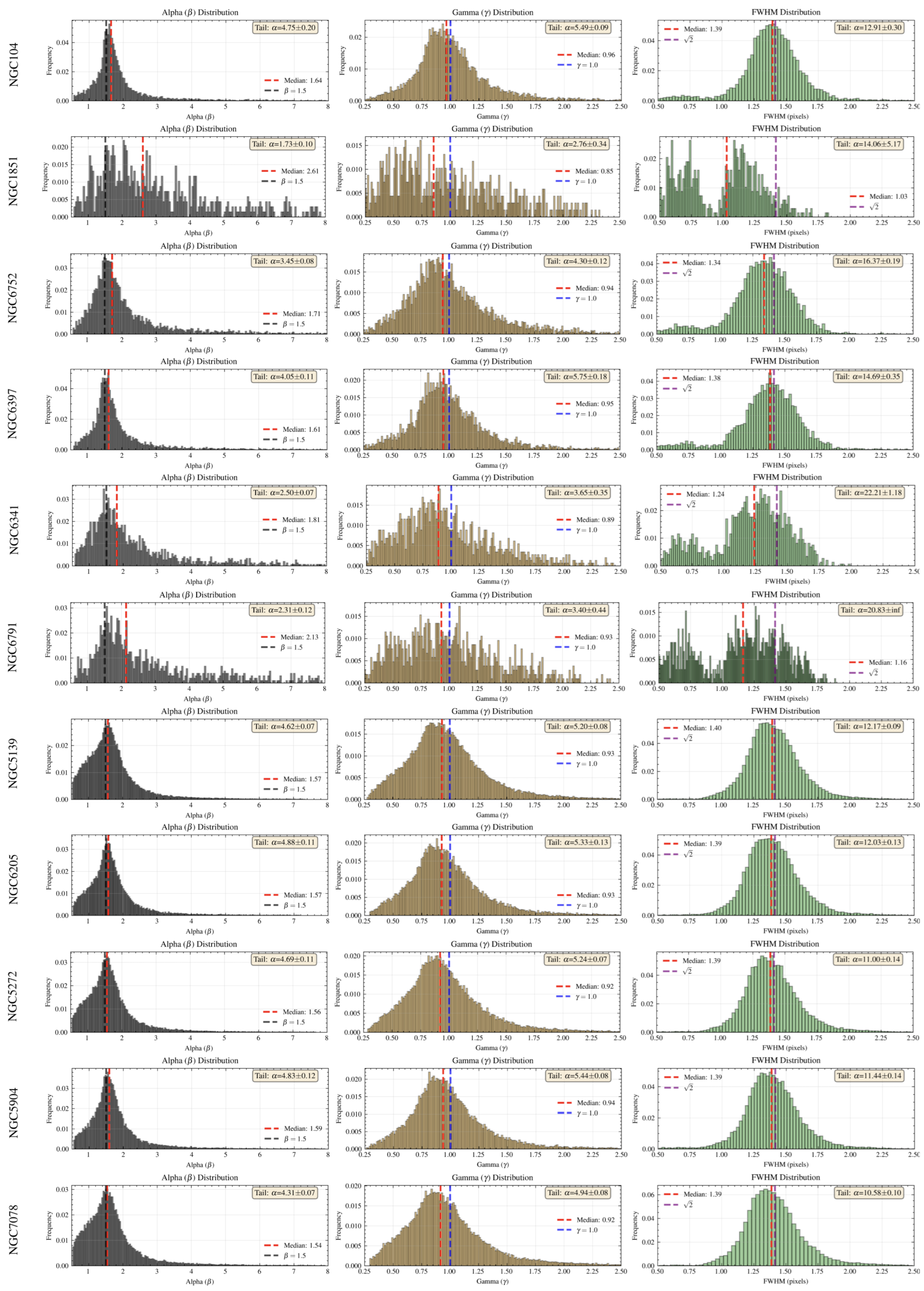
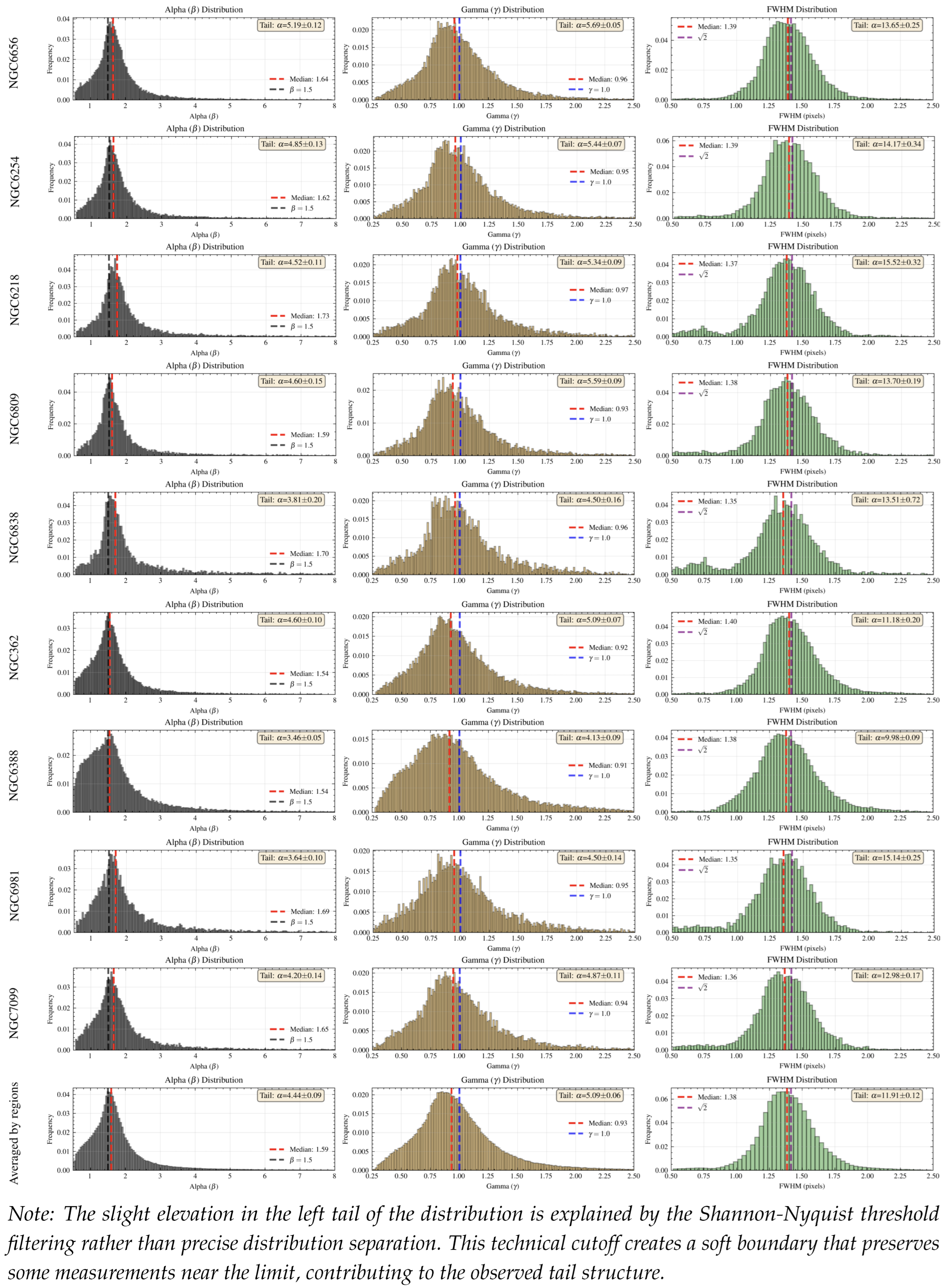
Appendix 19.4 Reproducibility and Open Science
All analysis code, data reduction procedures, and intermediate results are made publicly available. The analysis is designed to be reproducible by any programmer with standard Python skills within half a day of running the code cells. This transparency is essential for the scientific community to verify, critique, and extend these results.
Appendix 20 Mass is not the first entity: Logical Arguments
Appendix 20.1 Building on an Inverted Foundation is Problematic
The current foundation of physics has inverted the hierarchy of measurable (observable) entities. The electromagnetic spectrum of an object is more fundamental than its mass — it is literally a 2D picture that contains complete information about the physical system.
This section presents rigorous logical arguments demonstrating that mass cannot be a fundamental entity in physics, but rather emerges as a derived characteristic extracted from more primary electromagnetic phenomena.
Appendix 20.2 Information Asymmetry: The Fundamental Logical Argument
The most compelling argument against the primacy of mass is based on information asymmetry — a mathematically rigorous and empirically verifiable relationship between electromagnetic spectra and mass.
Appendix 20.2.1 Direct Observability vs Indirect Inference
A fundamental distinction underlies all physical measurements:
- The electromagnetic spectrum is the most directly observable phenomenon
- Mass is always indirectly inferred from other measurements, never observed directly
This observational hierarchy reflects a deeper information structure where the directly observable (EM spectrum) contains complete information about the indirectly inferred (mass).
Appendix 20.2.2 Mathematical Formulation
Consider the functional relationship between electromagnetic phenomena and mass:
- Forward function exists:
- Inverse function does not exist:
This is not a technical limitation but a fundamental mathematical property. The function f is well-defined and surjective (many-to-one), but not bijective (one-to-one). Therefore, the inverse function cannot exist.
Logical consequence: Since the EM spectrum contains strictly more information than mass, it must be informationally and ontologically primary.
Appendix 20.2.3 Why Dimensionality Alone Cannot Explain This Asymmetry
A critical objection might be: "Perhaps this asymmetry exists simply because the EM spectrum has higher dimensionality than mass (a scalar)." However, this explanation fails under rigorous analysis.
Counter-example: Even if we combine mass with multiple additional scalar parameters, we still cannot reconstruct the EM spectrum:
Fundamental reason: The EM spectrum contains qualitatively different information — it directly reflects the microstructure of matter (atomic energy levels, molecular bonds, quantum transitions). Mass is an integral characteristic — a "convolution" of all this complexity into a single number.
Analogy: Just as a detailed city map allows calculating the city’s area, but knowing the area + population + elevation cannot reconstruct the map. The map contains structural information that cannot be recovered from integral characteristics.
Appendix 20.3 Background and Distortions: The Transfer Function Perspective
We can conceptualize electromagnetic observations as deviations from a background electromagnetic state. In this framework:
- There exists a "background" electromagnetic field (vacuum state, cosmic microwave background, or thermal equilibrium)
- Physical objects create distortions or deviations from this background
- What we observe are these distortions acting as "transfer functions" in spectral space
- Mass represents a measure of how strongly an object distorts the background EM field
This perspective treats mass not as a fundamental property, but as a characterization of electromagnetic distortion — a secondary effect of primary electromagnetic phenomena.
Appendix 20.4 Practical Reality: The Airport X-ray Analogy
The airport security analogy perfectly illustrates the inverted hierarchy in our current understanding of physics.
Appendix 20.4.1 Airport Security Process
At airport security:
- Operator sees a colored 2D X-ray image of luggage contents
- From this image, the operator instantly determines: presence of metallic objects, their approximate shape, density, and can estimate mass
- The reverse is impossible: knowing only "luggage mass = 15 kg," the operator cannot determine what’s inside
Key insight: Security decisions (allow/inspect) are made based on the electromagnetic image, not mass. Mass is merely one characteristic that can be extracted from the image.
Appendix 20.4.2 Direct Parallel to Astrophysics
This is a precise analogy to astrophysics:
- Astronomers "see" the EM spectrum of a star
- From this spectrum, they extract mass, composition, temperature
- Having only mass, they cannot predict the spectrum
The airport analogy makes the abstract argument concrete and intuitive — everyone understands that the X-ray image is more informative than the weight measurement.
Appendix 20.5 Empirical Evidence from Stellar Astrophysics
Appendix 20.5.1 Overwhelming Reliance on Spectroscopy
The practical reality of modern astrophysics provides overwhelming evidence for the primacy of electromagnetic phenomena:
- The vast majority of stars are "weighed" exclusively through spectroscopy
- Parallax measurements are available only for the nearest stars (limited by Gaia to 1-2 kiloparsecs)
- Orbital dynamics is accessible only for binary stars where orbital motion can be observed
- For the remaining millions of catalogued stars, spectroscopy is the only method for mass determination
This is not a temporary technical limitation but a fundamental reality of observational astronomy. Distance and time scales make alternative methods impossible for the overwhelming majority of astronomical objects.
Appendix 20.5.2 Chemical Composition from Light Alone
The most striking example of electromagnetic primacy is the determination of chemical composition:
- From the EM spectrum of a distant star, we can determine exactly which elements are present
- This works for stars tens of thousands of light-years away
- We know the chemical composition more precisely than we know the mass
- The EM "fingerprint" is so specific that we can identify individual isotopes
This demonstrates that electromagnetic phenomena carry complete information about matter’s fundamental structure.
Appendix 20.5.3 Gravitational Waves: No Exception
The detection of gravitational waves by LIGO/Virgo experiments further confirms the universal pattern:
- Gravitational waves produce spacetime distortions of order
- These distortions are detected through laser interferometry
- The measurement relies entirely on electromagnetic radiation (laser light) to carry information about the distortion
- No alternative detection method exists that bypasses the electromagnetic channel
This observation reinforces that electromagnetic phenomena constitute the exclusive channel through which physical reality becomes accessible to measurement.
Appendix 20.6 Contradiction with Current Physics Paradigm
Appendix 20.6.1 Current Hierarchy in Physics
The standard physics paradigm places mass/energy as fundamental:
- Mass-energy equivalence: treats mass as a primary quantity
- Standard Model: Particle masses are fundamental parameters
- General Relativity: Mass-energy as the source of spacetime curvature
- EM spectroscopy: Treated as a "measurement tool" rather than primary reality
Appendix 20.6.2 Empirical Reality Shows the Opposite
However, empirical practice in physics demonstrates the reverse hierarchy:
- Mass is extracted from EM data, not independently measured
- EM phenomena determine mass, not vice versa
- When EM measurements and mass calculations disagree, we trust the EM data
- Particle "discovery" means observing characteristic EM signatures
This represents a fundamental paradigm inversion: what we treat as primary (mass) is actually secondary, and what we treat as secondary (EM phenomena) is actually primary.
Appendix 20.7 Philosophical and Theoretical Implications
Appendix 20.7.1 Redefining Fundamental Entities
If mass is a function of EM phenomena, then:
- Mass cannot be fundamental — it is a derived quantity
- The 2D EM "picture" contains complete physical description
- Mass is one parameter extracted from this complete description
- Physical reality is the EM field structure, not matter with mass
Appendix 20.8 Conclusion: The Inverted Foundation
Current physics is built on an inverted foundation where:
- The informationally poor (mass) is treated as fundamental
- The informationally rich (EM spectrum) is treated as secondary
- The derived quantity (mass) is placed at the base of theories
- The primary phenomenon (EM field) is considered a measurement tool
This inversion creates numerous conceptual problems and paradoxes in modern physics. The proposed framework corrects this hierarchy, placing electromagnetic phenomena in their rightful position as the primary physical reality from which all other quantities, including mass, are derived.
The fundamental insight: Mass is not an intrinsic property of matter but a measure of how matter deviates from the pure 2D electromagnetic state. The EM spectrum is the complete information; mass is merely one number extracted from this complete description.
Appendix 21 Empirical Argument From The Couch
Appendix 21.1 What Makes This Argument Particularly Strong
Section 19 discussed the characteristics of a strong scientific argument. That list was incomplete. Imagine if anyone could verify Special Relativity by examining their old photographs with a magnifying glass, understanding within hours which theoretical explanations best match observations, and then immediately benefit personally from this knowledge by enhancing their existing and future photographs without changing their camera. Such arguments and experiments are exceedingly rare and powerful. This section presents exactly such an experiment. This section also contains more standard scientific arguments. All code is provided and reproducible.
Appendix 21.2 Design of a Simple Experiment
The experimental protocol consists of the following simple steps:
- Configure a modern smartphone camera to save raw sensor data in monochrome mode (monochrome mode ensures experimental purity and reduces computational time)
- Take any ordinary photograph under normal lighting conditions
- Analyze the raw image data using the provided code (on a standard consumer laptop with GPU, unoptimized code requires approximately 1-2 minutes per raw photograph)
The simplicity of this protocol is deliberate — anyone with a modern smartphone can reproduce these results within hours, making this one of the most accessible fundamental physics experiments ever devised.
Appendix 21.3 Concrete Example
For this demonstration, an iPhone 14 Pro Max (neither the most expensive nor newest model) was configured to save raw sensor data. In the specific case of this device, this required enabling ProRAW and Resolution Control with Pro Default set to ProRAW Max, combined with monochrome mode. Each monochrome image captured through the 48-megapixel camera occupies 10-150 MB with a resolution of 6048×8064 pixels.
Under ordinary indoor lighting conditions, a standard interior scene was photographed. The complete raw file and analysis code are provided with this paper. A compressed version for publication appears below:
Appendix 21.4 What the Testable Theory Predicts
The testable theory, similar to the telescope section, predicts:
- Moffat-shaped Point Spread Functions (PSF) will demonstrate notable dominance over default models in key metrics solely by switching to physically correct PSF
- Absence of significant dependence on optics type, distance, and atmosphere (positive effect should be observed universally in pairwise comparisons)
- Immediate practical benefit from application
Figure A1.
Raw monochrome photograph captured with iPhone 14 Pro Max under standard indoor lighting conditions
Figure A1.
Raw monochrome photograph captured with iPhone 14 Pro Max under standard indoor lighting conditions

Figure A2.
Sample 1
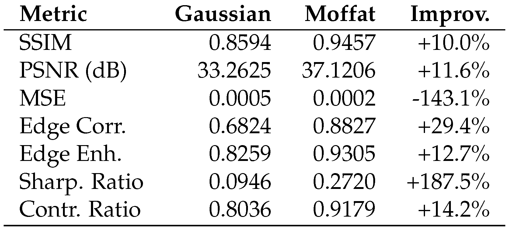
Figure A3.
Sample 2
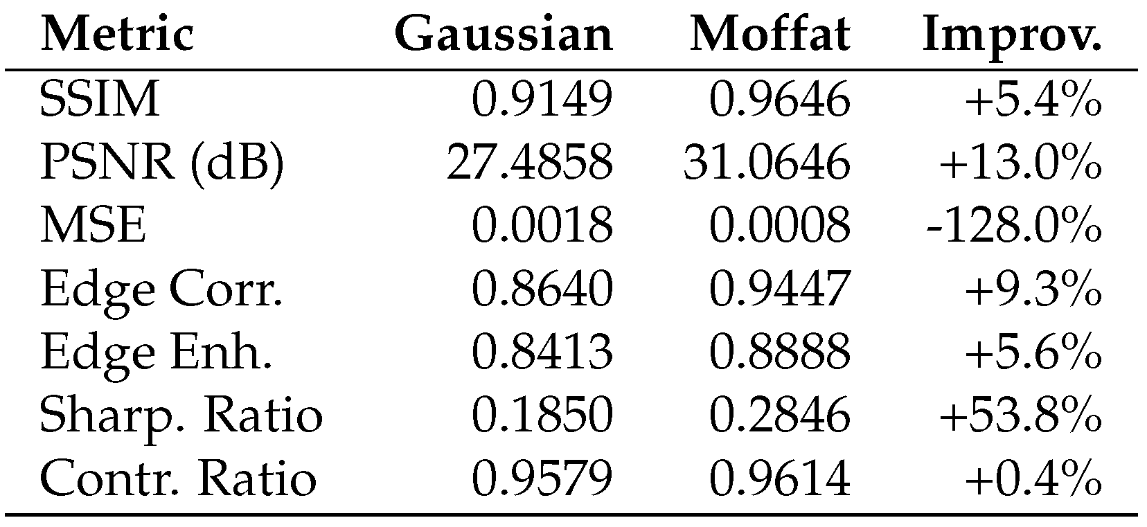
Figure A4.
Sample 3
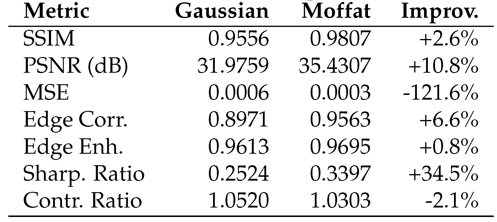
Figure A5.
Sample 4
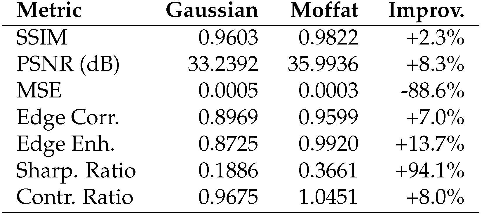
Figure A6.
Sample 5
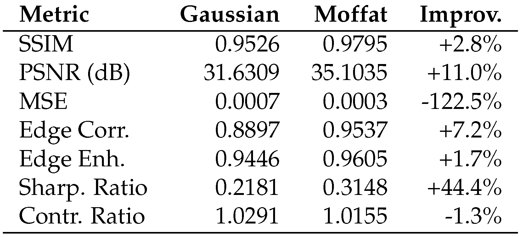
Figure A7.
Sample 6
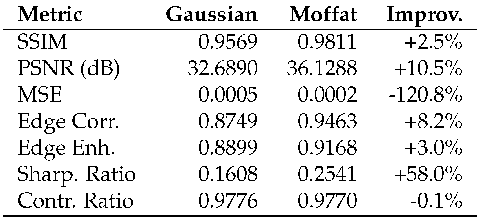
Appendix 21.5 What Default Theory and Practice Say
Appendix 21.5.1 Current Industry Standard
The photography and image processing industry universally employs Gaussian-based deconvolution algorithms:
- “Smart Sharpen” in Adobe Photoshop uses Gaussian assumptions
- Smartphone computational photography relies on Gaussian blur models
- Scientific image processing software defaults to Gaussian PSFs
- No major software offers Cauchy/Moffat-based deconvolution
- No theory predicts and explains Moffat dominance for non-astronomical images or provides theoretical recommendations for beta
Appendix 21.5.2 Theoretical Justification
The Gaussian assumption is justified by:
- Central limit theorem arguments for multiple scattering
- Mathematical convenience (Gaussian convolutions remain Gaussian)
- Historical precedent from film photography era
Appendix 21.6 Analysis Results
The deconvolution analysis yields striking results that directly test the fundamental nature of light propagation. Results comparing Gaussian and Moffat kernels on personal raw photos (details in the attached open code named B_clear) in full color variant (see figures A2-A11).
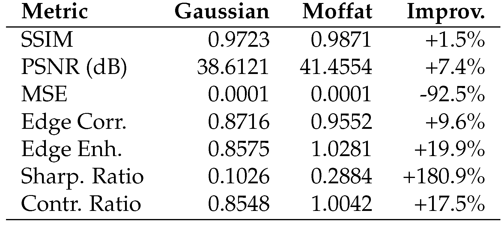
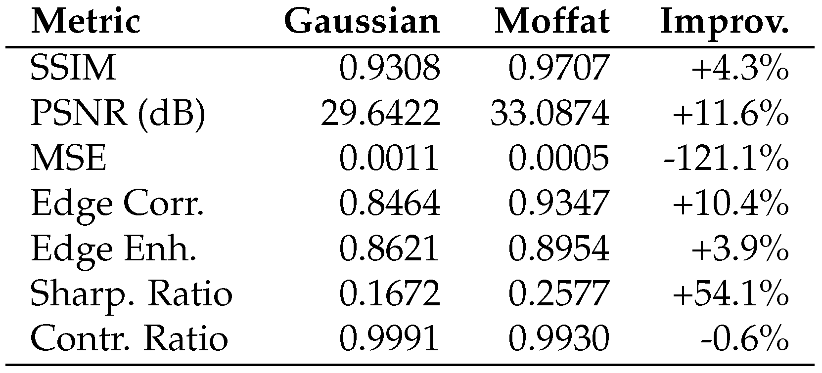
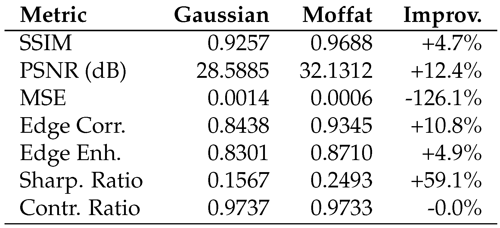
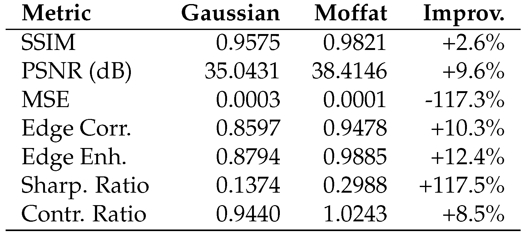
Figure A8.
Sample 7
Figure A9.
Sample 8
Figure A10.
Sample 9
Figure A11.
Sample 10
Appendix 21.7 Argument on Public Photographs with Compression
The observed effect is sufficiently strong that 2 public datasets with compression (JPG) containing ordinary public photographs taken on various mobile phones, with literally 30 randomly selected samples from each, yielded statistical significance. The images have different resolutions, were taken by different people in different locations on different devices, scenes, lighting conditions, different dominant colors, with and without motion blur, and all significant parameters in the samples vary. See code B_public_jpg.
Appendix 21.7.1 Dataset 1 Results

Table A1.
Statistical summary for Dataset 1 (30 samples)
| Metric | Gaussian | Moffat | Delta |
|---|---|---|---|
| SSIM (↑) | |||
| PSNR (dB) (↑) | |||
| MSE (↓) | |||
| Edge Correlation (↑) | |||
| Edge Enhancement (↑) | |||
| Sharpness Ratio (↑) | |||
| Contrast Ratio (↑) |
In both this subsection and the previous personal experiment, the distance to photographed objects was meters or tens of meters.
As evident, even already compressed photographs taken long ago can become significantly better simply from the proposed kernel change without sensor replacement. The effect is significant and the benefit is immediate and perceptible (such metric changes are visible to the eye). This is purely a matter of software processing.
Appendix 21.8 Argument Through Satellite
A public uncompressed photograph from a Maxar satellite in a single channel (monochrome image) was taken from the 2024 Turkey earthquake. Maxar satellites fly at an altitude of approximately 700km, with spatial resolution of 34cm × 34cm per pixel. Typical sizes of such images are 15000 × 15000 pixels. This is an example of one of the best civilian optics. Their working range is visible spectrum and near infrared. This exemplifies high-quality optics operating through atmospheric interference at extreme distances. Implementation available in MX_cl code.
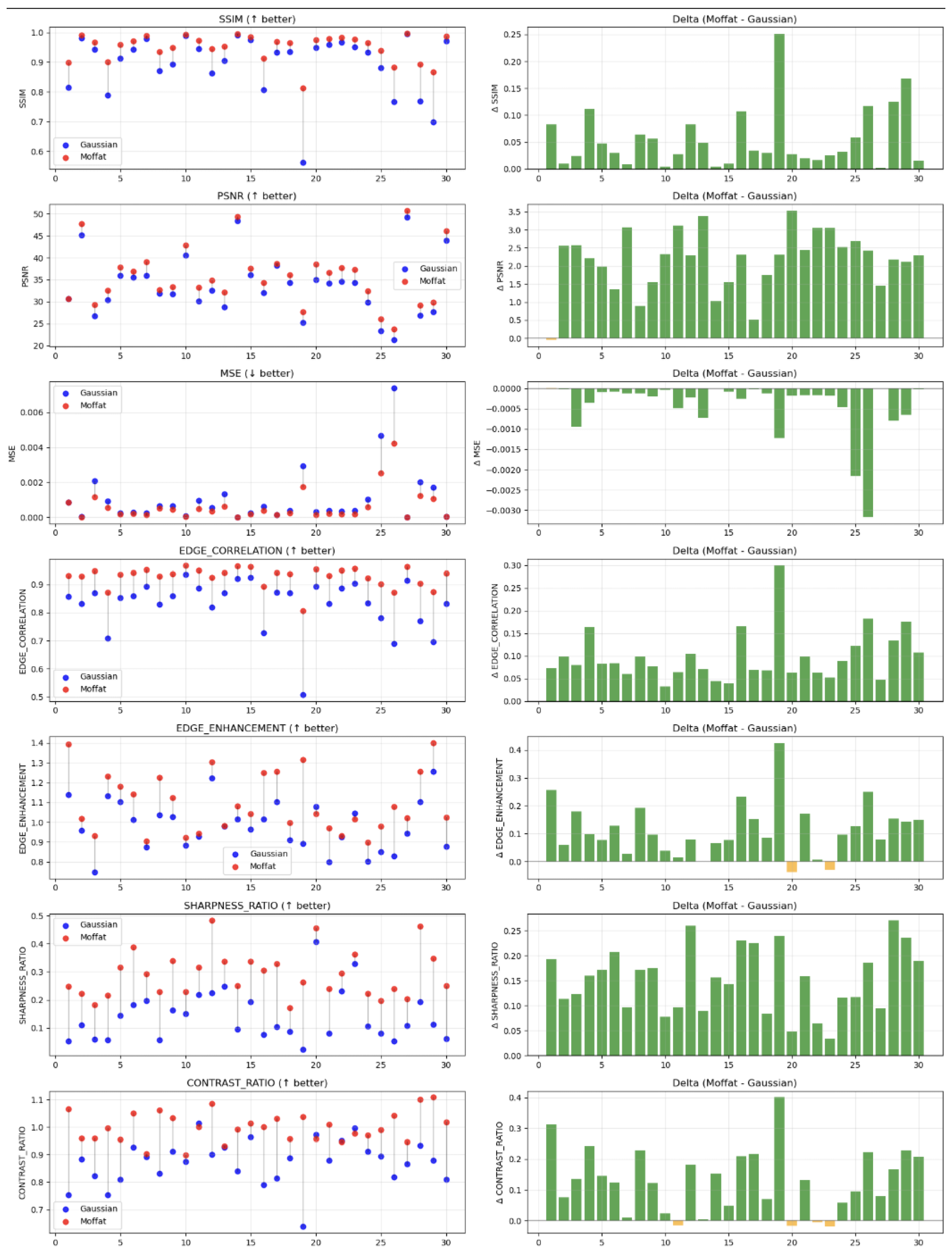
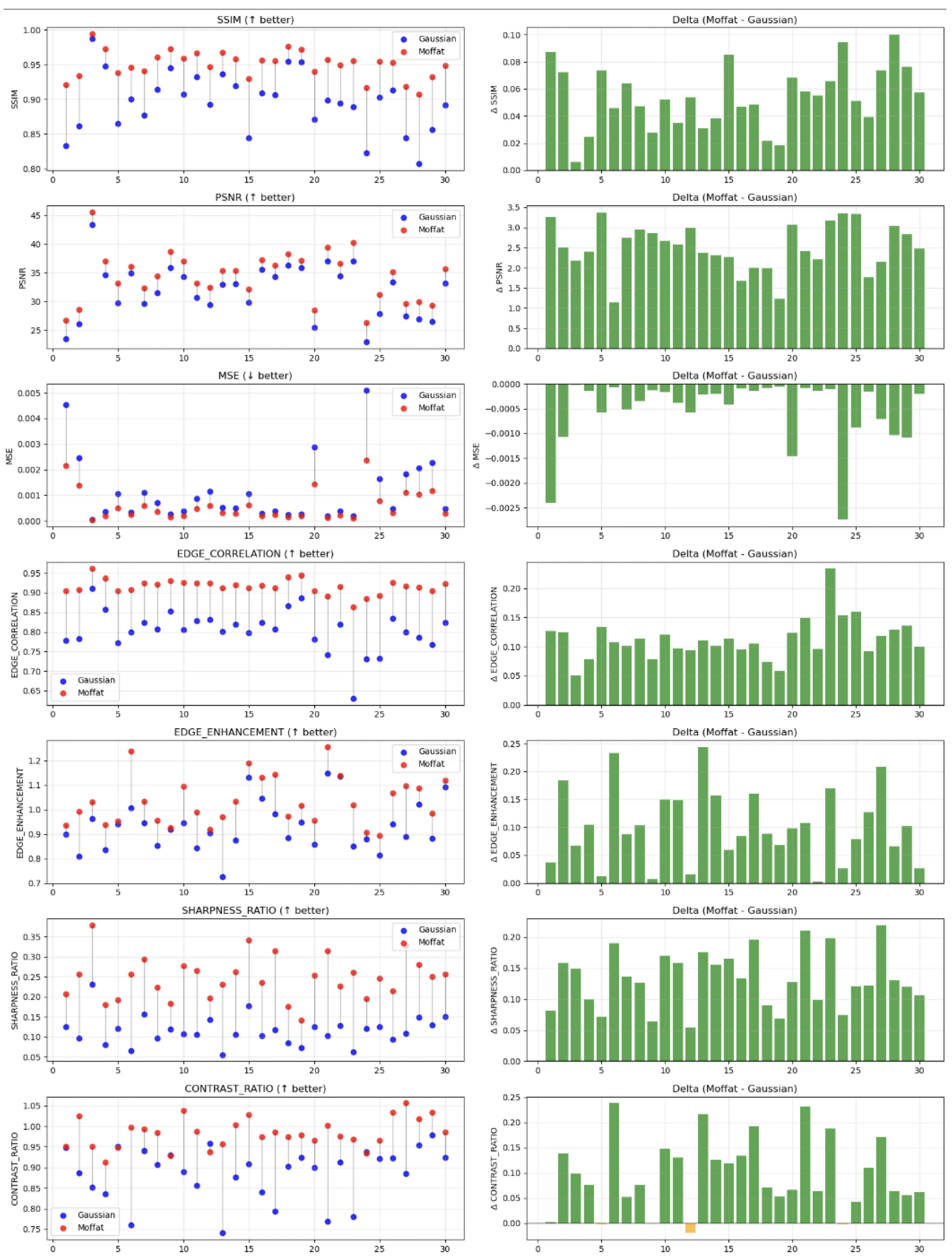
Figure A12.
Performance comparison on Dataset 1: Gaussian vs Moffat deconvolution across all metrics
Figure A12.
Performance comparison on Dataset 1: Gaussian vs Moffat deconvolution across all metrics
Figure A13.
Performance comparison on Dataset 2: Gaussian vs Moffat deconvolution across all metrics
Figure A13.
Performance comparison on Dataset 2: Gaussian vs Moffat deconvolution across all metrics
Table A2.
Statistical summary for Dataset 2 (30 samples)
| Metric | Gaussian | Moffat | Delta |
|---|---|---|---|
| SSIM (↑) | |||
| PSNR (dB) (↑) | |||
| MSE (↓) | |||
| Edge Correlation (↑) | |||
| Edge Enhancement (↑) | |||
| Sharpness Ratio (↑) | |||
| Contrast Ratio (↑) |
Table A3.
Detailed results table for satellite image deconvolution
| Metric | Delta | Best Gaussian | Best Moffat | (G-D) | (M-D) | (M-G) |
|---|---|---|---|---|---|---|
| SSIM | 1.0000 | 0.9778 | 0.9952 | -0.0222 | -0.0048 | +0.0173 |
| PSNR | 100.00 | 37.01 | 43.81 | -62.99 | -56.19 | +6.80 |
| Sharpness Ratio | 1.000 | 1.098 | 1.346 | +0.098 | +0.346 | +0.249 |
| Edge Ratio | 1.000 | 1.257 | 1.142 | +0.257 | +0.142 | -0.115 |
| Edge Correlation | 1.0000 | 0.9816 | 0.9977 | -0.0184 | -0.0023 | +0.0161 |
| Noise Level | 0.066 | 0.065 | 0.065 | -0.001 | -0.001 | -0.000 |
| Ringing Ratio | 0.000 | 1.211 | 1.116 | +1.211 | +1.116 | -0.095 |
| Iterations | 1 | 5 | 3 | +4 | +2 | -2 |
Point-like object fitting from a single photograph (995 objects analyzed) produced beta parameters with mean 2.639, median 2.367, and standard deviation 0.884. Although less precise than dedicated stellar photography for beta estimation, these results consistently indicate values near 2 rather than 4.
Appendix 21.9 Why This Matters
Appendix 21.9.1 Immediate Cheap Personal Verification
Unlike abstract physics experiments requiring billion-dollar installations, this experiment:
- Can be performed by anyone with a smartphone
- Yields results within hours, not years
- Offers immediate practical benefits (better photographs)
- Requires no specialized physics knowledge to evaluate
Appendix 21.9.2 Universal Applicability
The implications extend far beyond amateur photography:
- Medical imaging: improving CT, MRI, X-ray, PET (right now anyone can replace the software processing of such medical data and see more details, which will save lives of enormous numbers of people through more accurate diagnosis)
- Astronomy: enhancing telescope image resolution and revealing new real details (as demonstrated in the 19 section)
- Microscopy: cellular and molecular imaging
- Satellite imagery: Earth observation
- Any field where electromagnetic signal carries information
Appendix 21.9.3 Economic Impact
The potential economic value is enormous:
- Trillions of existing digital images can be enhanced
- Future imaging systems can be optimized from first principles
- Computational requirements can be reduced (Moffat consistently converges faster, parameter count is the same as default model)
- Image quality improvement without hardware changes
Appendix 21.10 Conclusion
This “from the couch” experiment presents a new paradigm in fundamental physics verification — one where anyone can test deep theoretical predictions using everyday devices and immediately benefit from the results. The consistent superiority of Moffat/Cauchy-based image processing across all tested conditions provides strong empirical support for the two-dimensional nature of electromagnetic phenomena and their adherence to Cauchy distribution law.
The fact that billions of people carry devices capable of testing these fundamental principles, yet current technology ignores them in favor of inferior Gaussian models, represents both an enormous opportunity and evidence for the revolutionary nature of these discoveries. Every smartphone photograph processed with Gaussian assumptions is empirical evidence waiting for proper analysis — and improvement — using correct physical principles.
This accessibility transforms abstract physics into tangible personal experience, making verification of fundamental laws of nature as simple as taking a photograph and running the provided code. In the history of physics, few experiments have offered such a combination of theoretical depth and practical immediacy.
Appendix 22 Light the Candles: The Universe Is Not Running Away
The hypothesis of the expanding universe rests on the following arguments:
- the actually observed redshift (z), whose distance estimates agree with those obtained via parallax and other methods for nearby objects; the redshift resembles the Doppler effect
- the only alternative explanation known as the tired light hypothesis (that photons as particles collide with microparticles and lose energy along the way) was rejected due to the fact that image sharpness does not degrade with distance (the image of an object does not blur)
- the expansion hypothesis is indirectly supported by the CMB if interpreted as an echo of the early inflationary phase
In this section, these assumptions will be called into question. All details are provided in the attached open C1 code, written so that anyone can independently verify the results within hours.
Appendix 22.1 Observed z of Quasars Depends on Frequency
Using only easily accessible SDSS data (without the precision of DESI) and a regular laptop, it is possible to observe systematic deviations of residuals from the z values in the catalog within hours. These deviations do not follow a normal distribution and depend on wavelength. This single observation unequivocally refutes the hypothesis of the Doppler nature of redshift.
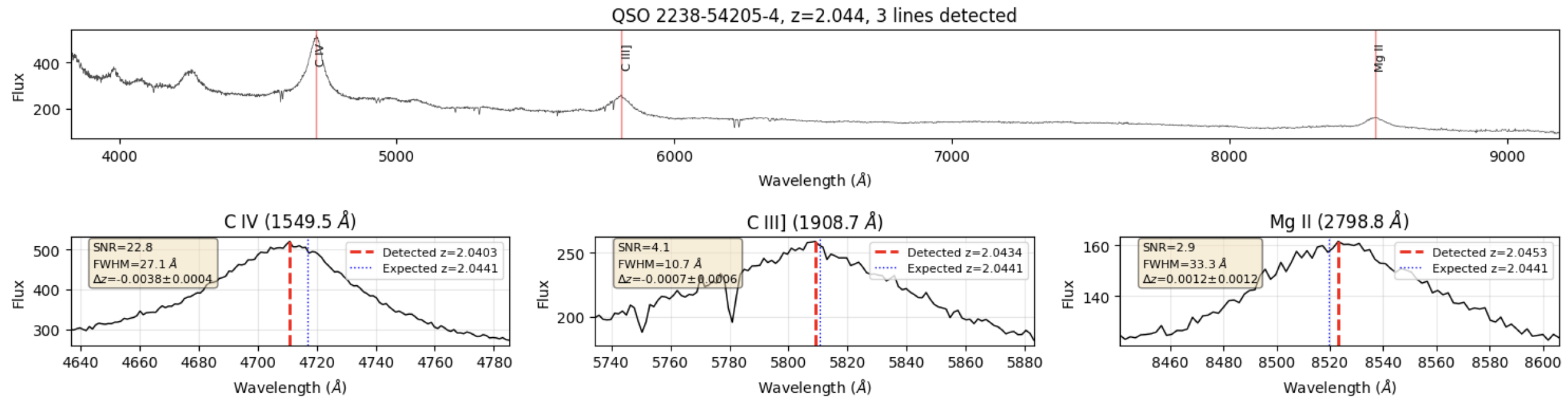
Figure A14.
Example to illustrate systematic deviation in the spectrum of 1 quasar
The Kruskal-Wallis statistical test confirms that these are different distributions with a clear dependence on wavelength. The precise analysis reveals that the deviations (medians) exhibit a Pearson correlation of 1.00 with respect to the logarithm of the rest wavelength, while the mean values show a Pearson correlation of 0.96. This establishes a definitive logarithmic dependence.
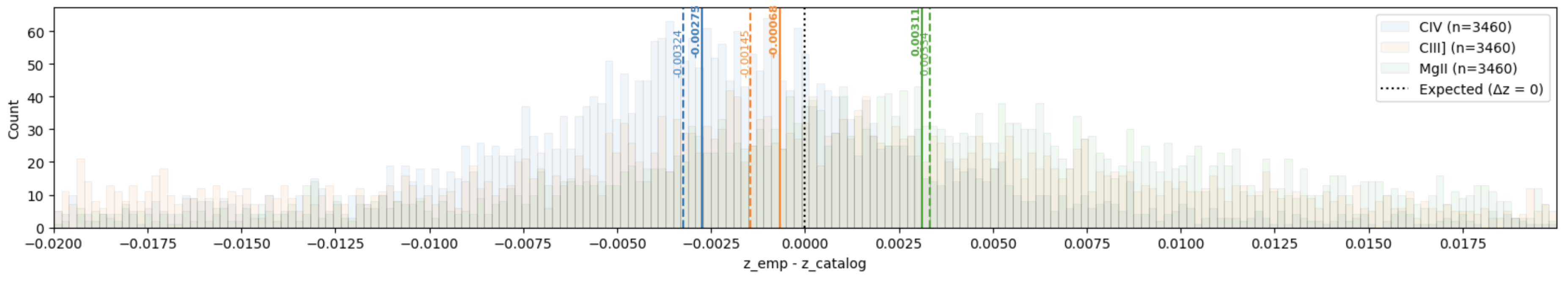
Figure A15.
Visualization of all quasars from SDSS with and where all 3 indicators were found.
Critically, the observed pattern manifests as frequency-dependent power-law suppression, precisely matching the predictions of the dimensional theory presented in this work. The logarithmic dependence corresponds to exponential suppression of the form , where represents the dimensional deviation parameter.
Furthermore, detailed directional analysis reveals that the slopes exhibit systematic variation with sky position, indicating anisotropic dimensional structure of space — a phenomenon entirely unpredicted by standard cosmology but naturally emerging from variable dimensional flow theory.
Doppler logic provides a reasonable first approximation but fails rigorous tests with modern precision data. The expansion of the universe and the necessity for dark energy are brought under serious doubt by these findings.
This investigation into the fundamental nature of cosmic redshift continues, with implications extending far beyond cosmology to the very structure of space and time.
Appendix 23 Laughter from the Ferris Wheel
Appendix 23.1 The Ballerina’s Pirouette
Recall or look up the famous visual illusion by Nobuyuki Kayahara featuring a spinning ballerina. The figure lacks depth information, making it impossible to unambiguously determine the direction of rotation and speed. The speed could always be larger by a multiple of complete rotations (for example, what appears to be a 30-degree clockwise rotation in the next frame could actually result from any rotation of degrees for any integer n).
Appendix 23.2 The Universal Roulette
Imagine observing the rotation of a roulette wheel in a casino. In the simple case, one watches from a camera suspended above the axis of rotation, seeing the entire circle without distortion. One observes the position of the first cell and believes the rotation system is completely understood, as each subsequent frame appears to show the cell shifting by 10 degrees clockwise. However, the same problem as with the ballerina emerges: ambiguous relationships between discretization and angular velocity (for instance, each frame might indicate a 180-degree rotation, and in such a system it would be logical to seek the minimum possible energy configuration, but no preferred direction of rotation can be chosen).
Now imagine observations from the side, from the perspective of a typical player. Information is inevitably lost during projection, and the question of depth estimation is not always resolvable.
Consider a time-ordered series of photographs of the Andromeda galaxy (arranged by a photographer from old to new snapshots, who assures that they were taken at equal time intervals). The problems with determining speed and direction of rotation are identical. If redshift cannot be interpreted exclusively through the Doppler effect, then there is no source of depth information. Estimates of angular velocity become much less straightforward and require stronger reliance on the tenuous anthropic principle (it seems strange to think that a distant galaxy chooses its speed to make observations more convenient).
Arguments that galaxies rotate "somehow incorrectly" (have unexpected rotation parameters) against the backdrop of not really knowing how to unambiguously determine their rotation parameters sound inappropriate.
Appendix 23.3 The Revenge of Ptolemaic Epicycles
How can any theory claiming to fundamentally explain space-time ignore the fact that the only path from time leads to Fourier analysis and 2D rotations? Circular rotation is the most misunderstood mechanism. This section concerns empirical arguments and an attempt to reconceptualize this phenomenon.
Almost everything observable at all scales appears to be rotating. Explanations through unestablished random causes that once, somehow, sometime in the past distributed impulses to everything are weak and barely differ from a version about a god who arranged everything and pushed each object as he decided without reason. Electric motors (which use rotation and electromagnetic fields) have the highest efficiency among known devices. It is a huge blind spot that the phenomenon of rotation is considered understood and practically ignored.
Appendix 23.4 Cryptanalysis of Enigma 2.0
Rotation is a codec (encoder-decoder) that allows non-2D objects (both higher and lower dimensional) to synchronize through a 2D electromagnetic channel.
The fact that rapid isotropic rotation is indistinguishable from isotropic radiation can be rigorously demonstrated. A rapidly and uniformly rotating beam in a 2D plane is indistinguishable from uniform emission in a 2D plane from a point, and this can be proven for the general case.
Appendix 23.4.1 Mathematical Foundation of the Dimensional Codec
The intuitive ideas about rotation as a universal mechanism for dimensional encoding can be made mathematically precise through the theory of spherically symmetric distributions and their Fourier transforms. The key insight is that gnomonic projection of isotropic directions produces distributions whose spectral representations are dimension-agnostic, allowing Fourier analysis to serve as a codec between different dimensional spaces.
Setup and Vocabulary. The probability/Fourier transform convention is used:
A random vector is spherically symmetric (isotropic) if for every orthogonal matrix Q, .
The isotropic multivariate Cauchy in with location and scale is:
Gnomonic (central) projection of the unit sphere : for with ,
Theorem. Let . For any ,
has the d-dimensional Cauchy law with density (Cauchy-pdf) for , , provided (which occurs almost surely). Equivalently, if is uniform on , then has the same law.
Corollary. The distribution of depends only on d (the target dimension), not on D as long as .
Theorem. For the isotropic Cauchy in ,
The functional form of is independent of d.
Although (CF) hides d, the inverse Fourier transform depends on d. For a radial in ,
where is the Bessel function.
Proposition. Let be any isotropic Cauchy in with the same . Then all coincide pointwise:
Thus the Fourier transform identifies the family of isotropic Cauchy distributions across all dimensions to the same radial exponential in frequency.
Proposition. Given the common spectral profile , the inverse transform in dimension d yields the isotropic Cauchy density in . Different choices of d produce different spatial laws with tail power .
The Codec Interpretation.
- "Upstream" encoding: start with an isotropic direction on and gnomonically project to ⇒ result is Cauchyd.
- Codec step: move to frequency domain ⇒ dimension information is encoded in the universal form .
- "Downstream" decoding: choose a target dimension and invert in ⇒ recover .
In this sense, Fourier transformation acts as a codec between isotropic rotators across dimensions: the spectral representation is universal; the dimension is encoded as a parameter in the inverse operation.
The entire framework extends to all spherically symmetric -stable laws:
with Cauchy as , Gaussian as . The spectrum remains dimension-agnostic; the inverse Fourier transform restores the dimensional information.
Fundamental Nature of 2D Encoding. Every Fourier component represents a 2D rotation in the complex plane, regardless of the dimension of the original space. This reveals that Fourier transformation is fundamentally a 2D codec: all dimensional information is encoded through 2D rotational structures, making the electromagnetic channel (which is inherently 2D) the natural medium for this universal dimensional codec.
Extension to Non-Integer Dimensions. Critically, this mathematical framework remains valid for non-integer dimensions. The gamma function is well-defined for all positive real z, the characteristic function is independent of dimensional parameters, and spherical volume formulas extend naturally to fractional dimensions through . This mathematical consistency suggests that the rotational codec operates equally well for fractional dimensional spaces, expanding its applicability to fractal structures and systems with effective non-integer dimensional parameters.
Appendix 23.5 Breaking Mad
The so-called “uncertainty principle” is usually presented as if the Universe deliberately hides information from us. In fact, it is only the Fourier codec in disguise.
- Pure mathematics (Cauchy–Schwarz inequality in Fourier analysis) givesfor any square-integrable signal.
- Physics adds the empirical link . Substitution yields
- Similarly, using for wave number k, one obtains
Thus the famous is not a magical law about “unknowability,” but the most elementary fact about the Fourier codec applied to the electromagnetic channel. The numerical value of ℏ has no deeper mystery than the width of railway tracks: it comes from conventions of units and history, not from cosmic fine-tuning. The world is not hiding — our channel simply encodes information this way.
Appendix 23.6 The Ballerina’s Second Pirouette
The ballerina’s pirouette provides a direct demonstration of information-theoretic constraints operating in physical systems. When a spinning ballerina pulls in her arms, the traditional explanation invokes conservation of angular momentum: remains constant, so decreasing moment of inertia I requires increasing angular velocity .
However, this mechanical explanation obscures the deeper information-theoretic mechanism at work. The same quantitative result emerges inevitably from the Kotelnikov-Shannon-Nyquist sampling theorem applied to the dimensional codec.
Spectral Band Displacement: When the ballerina’s spatial projection compresses by factor k, all spatial frequency components shift upward by the same factor. If the original spatial spectrum was band-limited to frequency , the compressed configuration has maximum spatial frequency .
The Reading Speed Requirement: When spatial information becomes compressed, the system must "read" it faster to avoid missing details. If the ballerina’s spatial frequencies double due to compression, the temporal sampling must double to keep up. If they increase tenfold, sampling increases tenfold. This is like trying to read text that suddenly becomes smaller — you must scan faster to process the same information per second.
This fundamental requirement is captured by the Shannon-Nyquist theorem: to distinguish the shifted spectral bands without aliasing artifacts, the temporal sampling frequency must satisfy:
Since the rotational frequency serves as the temporal sampling rate for the 2D electromagnetic channel, the system must increase by factor k to maintain information fidelity.
Real-Time Information Constraint: This is not a consequence of mechanical forces or conservation laws inherited from past initial conditions. The acceleration occurs because the compressed spatial configuration creates higher-frequency spectral content that exceeds the channel’s current sampling rate. The Kotelnikov-Shannon-Nyquist theorem mandates increased temporal frequency to avoid information loss through aliasing.
The ballerina speeds up not because "angular momentum is conserved," but because the 2D electromagnetic channel requires higher sampling rates to encode the compressed spatial information without distortion. The rotational acceleration is an active information-processing requirement, not a passive mechanical consequence.
This information-theoretic perspective explains why rotational acceleration appears instantaneous with spatial compression — the sampling rate adjustment is a real-time channel requirement, not the result of force integration over time. The same mathematics that governs digital signal processing governs the ballerina’s spin: spatial compression shifts spectral bands rightward, demanding proportional increases in temporal sampling frequency to satisfy the Nyquist criterion.
Appendix 24 The Comeback of Black Furnaces
The so-called “ultraviolet catastrophe” was never a catastrophe of nature but only of the model. To see why Planck’s quantization worked — and why it looked like a miracle at the time — one must look not at metaphysical claims about the discreteness of matter, but at the Fourier channel and the statistics it enforces.
Appendix 24.1 Why the catastrophe appeared
Classical theory assumed that each frequency mode in a cavity carried an equal average energy (equipartition). This worked well for long wavelengths, but as frequency increased the model predicted that each additional mode stored the same “average,” leading to an infinite total energy. Experimentally, however, blackbody spectra were smooth, finite, and reproducible. The divergence was not in nature — it was in the Gaussian assumption that such averages exist.
Appendix 24.2 Enter Cauchy
Geometrically, isotropic directions projected onto a line produce the Cauchy distribution:
Unlike the Gaussian, the Cauchy has no finite mean or variance. And crucially, it is stable: if , then the average is still . No matter how long you ”observe” or how many samples you collect, the mean does not converge. There is no “true average energy per mode” to be found — it simply does not exist.
Appendix 24.3 Fourier makes discreteness inevitable
Any real measurement is time-limited. A window of duration T produces a discrete Fourier spectrum with spacing . Longer observation narrows the lines, but does not remove discreteness. Thus the energy of cavity modes cannot be distributed as a continuous Gaussian average; it must be encoded in discrete packets tied to frequency.
Appendix 24.4 Why Planck’s trick worked
Planck introduced the rule
restricting energy exchange to packets proportional to frequency. He did not know the language of stable laws, but his quantization exactly matched what the Fourier–Cauchy channel enforces:
- Fourier ⇒ discrete frequencies for finite windows,
- Cauchy ⇒ no Gaussian averages over modes,
- ℏ⇒ the scaling constant between frequency and energy.
Quantization was not a metaphysical leap but the natural coding rule of the channel.
Appendix 24.5 Why ℏ does not drift with longer observations
The uncertainty inequality
is pure Fourier mathematics. With , it becomes
Observing longer () narrows and hence , but the proportionality constant ℏ is fixed: it is the calibration between mathematical frequency and physical energy. Changing ℏ would be equivalent not to “finding a different universe,” but to redefining what we call a joule.
Appendix 24.6 The lesson
The “catastrophe” was a ghost born of Gaussian assumptions. Planck’s success was not magic but an effective recognition of the Fourier–Cauchy codec at work. Quantization is not an axiom about the ultimate discreteness of matter: it is the natural behavior of the electromagnetic channel under finite observation. The black furnaces never exploded; they were simply speaking a statistical language physicists of the 1900s did not yet understand.
Appendix 25 Classical Dynamics of Shadows
Zeno was right: motion can be understood as a sequence of filters and transfer functions. Classical mechanics is not about mysterious "forces" but about how nature selects and transmits modes through a spectral channel.
From Newton to Hamilton, from Lagrange to Feynman and Frieden, every formulation can be seen as a description of filters acting on frequency space.
Appendix 25.1 Newton’s Laws as Filters
First Law. Uniform motion corresponds to a trivial filter passing only the zero-frequency mode (). In spectral language, inertia means that once a mode is present, it passes through unchanged.
Second Law. Acceleration corresponds to a quadratic filter, since turns into in Fourier space. This law selects resonant frequencies: only modes consistent with force balance survive.
Third Law. Action and reaction express spectral reciprocity: every filter has its dual, enforcing conservation and symmetry across the channel.
In this sense, what Newton formulated as "laws of motion" are shortcuts to describing the spectral filtering of nature. Linear motion is nothing but a -filter on the proper mode, while acceleration is the quadratic filter that suppresses the rest.
Appendix 25.2 Lagrange’s Principle as Spectral Optimization
The Lagrangian formalism replaces forces with a balance of energy terms:
In Fourier space, each contribution becomes a weight on a frequency component:
- Kinetic energy ,
- Potential energy .
The action is then a quadratic functional of the spectrum:
The principle of least action, , means: the system selects that spectral distribution which minimizes the total cost of frequencies.
- In time domain: the trajectory is optimized.
- In frequency domain: the filter is tuned to pass only the “cheapest” spectral mode.
Thus, Lagrangian mechanics can be seen as an optimal filtering problem: among all possible frequency channels, the one realized by nature is that which minimizes the global spectral cost.
This makes the variational principle equivalent to the Wiener filter in signal processing: optimal transmission of signal with minimal noise and distortion.
Appendix 25.3 Hamilton’s Principle as Phase Evolution
The Hamiltonian formulation rewrites dynamics in terms of canonical variables :
In the spectral representation, evolution under the Hamiltonian corresponds to a pure phase rotation:
with determined by the Hamiltonian spectrum.
Thus, the Hamiltonian is not a filter of amplitudes but a phase operator:
- It preserves the spectral magnitudes ,
- It only shifts phases according to the energy of each mode.
This is exactly the action of an all-pass filter in signal processing: the spectrum remains intact, but its phase portrait rotates in time.
- Newton selected the allowed modes.
- Lagrange optimized the spectral cost.
- Hamilton now governs their coherent phase evolution.
In this sense, Hamiltonian mechanics describes the phase choreography of spectral components. It is the operator that ensures consistent interference and conservation, turning dynamics into structured rotations in frequency space.
Appendix 25.4 Feynman’s Path Integral as Superposition of Filters
Feynman’s formulation replaces a single trajectory with the sum over all possible histories:
Every path contributes as if it were a distinct filter applied to the spectrum. The weight of each filter is given by the phase factor .
In this language:
- Newton imposed a sharp mode selector.
- Lagrange minimized the spectral cost.
- Hamilton rotated the phases coherently.
- Feynman now allows all filters to act simultaneously, letting interference eliminate the inconsistent ones.
The stationary-phase principle explains why classical paths emerge: where the phase oscillates rapidly, contributions cancel; where the phase is stationary, contributions add coherently.
Thus, the Feynman path integral is a superposition of all possible filters, with destructive interference suppressing the unphysical channels. What remains is exactly the same classical dynamics already described by Newton, Lagrange, and Hamilton, but now derived from a deeper spectral principle.
Appendix 25.5 Frieden’s EPI as Informational Bandwidth Balance
Frieden reformulated physics in terms of information. He distinguished two quantities:
- I : the Fisher information available in the observed data,
- J : the structural information carried by the system itself.
The EPI principle states:
In spectral language, this is a statement about bandwidth: the physical filter must balance the information it transmits with the constraints of its internal structure.
- Newton: selected the allowed modes.
- Lagrange: minimized the spectral cost.
- Hamilton: preserved amplitude, evolved phase.
- Feynman: summed over all filters, interference chose the stable ones.
- Frieden: ensures that the resulting filter achieves optimal information transfer, no more and no less than the structure allows.
Thus, EPI is not a new law but the informational expression of the same filtering logic. It reveals that nature’s spectral filters are tuned at the balance point between maximum distinguishability (data) and minimum redundancy (structure).
Appendix 25.6 The Unruh Effect Will Be Found
The Unruh effect predicts that an observer with uniform acceleration a perceives the vacuum as a thermal bath with temperature
In the spectral–filter view this becomes transparent:
- Uniform motion () corresponds to a transparent filter: vacuum modes interfere coherently and cancel to “nothing.”
- Acceleration reshapes the filter: frequency modes are shifted and stretched.
- This deformation opens a stationary passband of modes which no longer cancel.
- The observer perceives this surviving spectrum as thermal radiation.
Thus, Unruh temperature is not a new entity but the natural consequence of how acceleration alters spectral filtering. It is the same logic that already underlies Newton’s mode selection, Lagrange’s cost minimization, Hamilton’s phase evolution, and Feynman’s interference principle. Frieden’s EPI then states that the balance of information between the vacuum field and the accelerated observer shifts, yielding a nonzero thermal signal.
From this perspective, the Unruh effect is not exotic but inevitable. It will eventually be confirmed experimentally, as it is simply the manifestation of acceleration as a spectral filter that reveals hidden modes of the vacuum.
Appendix 25.6.1 On Hawking Radiation
Hawking’s prediction of black hole radiation is often presented as a close analogue of the Unruh effect. Yet in the spectral–filter interpretation the two phenomena are fundamentally different. Unruh radiation arises because acceleration changes the observer’s filter on the vacuum spectrum, making a thermal band unavoidable. Hawking’s case, however, involves the global geometry of spacetime near the horizon, which acts only as a truncation of modes rather than a genuine generator of new ones.
The apparent thermal spectrum at infinity may thus be a coordinate artifact rather than a physical flux of particles. In this view, Hawking radiation may never be found, not because of experimental limits, but because it does not exist as a real emission process. Only the Unruh effect remains as the true spectral–thermal link between motion, acceleration, and temperature.
Appendix 25.7 Speed as Spectral Correlation
Consider a mode on the space–time Fourier plane . Normalize frequency by c: . Then straight lines
have slope . For a wavepacket with dispersion the local slope is
so speed is geometry: the tilt of the spectral ridge.
Appendix 25.7.1 Correlation reading
Let be the (whitened1) 2D spectral density of a wavepacket concentrated along an approximately linear ridge. The Pearson correlation of
then estimates the effective transport speed:
(when the ridge is near-linear on the bandwidth of interest). Intuitively, quantifies how tightly temporal and spatial harmonics co-vary.
Appendix 25.7.2 Canonical cases
- Pure transport: spectrum (delta-ridge), hence exactly.
- Light in vacuum: , ridge at , .
- Massive relativistic field: ; the ridge tilts below , giving locally.
- Schrödinger (free): parabolic ridge; around carrier , and on the local bandwidth.
- Diffusion/heat: is imaginary ⇒ no real ridge on ; there is no transport correlation to identify (consistent: diffusion smooths but does not carry).
Appendix 25.7.3 Practical recipe
Given from data: (i) normalize to units, (ii) whiten marginals, (iii) compute over the band of support. Then (use local in dispersive media).
Appendix 25.7.4 Notes
(i) Distinguish phase vs group velocity: uses global slope, uses local slope; the correlation estimate tracks the local group transport. (ii) In strongly curved ridges, compute in short k-windows to get . (iii) For anisotropic noise floors, perform a PCA/whitening step before estimating to avoid bias.
Appendix 25.8 Cauchy, Fourier, and the Lorentz Factor
The Cauchy distribution is special because its Fourier transform has a simple exponential form. For the centered case one has
Thus the Cauchy distribution in the time domain corresponds to an exponential low-pass filter in the frequency domain. The scale parameter controls the rate of spectral decay.
Now note that Lorentz time dilation rescales . Under Fourier transform,
so the spectral envelope acquires exactly the Lorentzian broadening familiar from Cauchy profiles.
In other words:
- The Cauchy distribution exponential spectral cutoff.
- Lorentz factor scaling of that cutoff.
- Together, relativity inherits the same analytic structure as Cauchy–Lorentz filtering.
This explains why the Lorentz factor in mechanics, the Lorentzian spectral line, and the Cauchy distribution are not separate coincidences, but different projections of the same analytic property:
Cauchy + Fourier = Lorentz scaling.
Appendix 26 Dissecting Maxwell’s Demon
Temperature is the width of the filter in the frequency domain of the EM spectrum. Thermal conductivity is the height of the filter. The verification zone is in that from models of the catalog of filters from DSP, the unfound ones should be found experimentally. The “mystical” arrow of time and the last t in the basic equations from the second principle of thermodynamics become extremely understood (spectrum addition is a unidirectional operation).
Appendix 26.1 Boltzmann’s Legacy and the Last Asymmetry
Ludwig Boltzmann pioneered the statistical understanding of thermodynamics, introducing the revolutionary that connected microscopic states to macroscopic entropy. His work presaged quantum mechanics through discrete energy levels and statistical ensembles. Yet his second law – the only fundamental physical equation where time enters asymmetrically – remained haunted by the reversibility paradox: how do time-symmetric microscopic equations produce irreversible macroscopic behavior?
The standard resolution invokes special initial conditions – the Past Hypothesis positing low entropy at the universe’s beginning. This transforms thermodynamics into cosmology, making the arrow of time a brute fact about boundary conditions rather than a derivable consequence of dynamics. Every other fundamental equation in physics – Newton’s, Maxwell’s, Schrödinger’s, Einstein’s – treats past and future symmetrically. Only thermodynamics breaks this symmetry, and only through an axiom about the universe’s birth.
Appendix 26.2 Maximum Entropy Method: Removing Time from Thermodynamics
The Maximum Entropy Method (MEM) offers a reconceptualization. When constructing spectral densities from time series data, MEM employs autoregressive (AR) processes that are inherently time-symmetric:
This formulation treats past and future equivalently – the AR coefficients remain unchanged under time reversal. The resulting spectral density maximizes entropy subject to autocorrelation constraints, yielding the least biased estimate compatible with observations.
Critically, MEM replaces Boltzmann’s time-asymmetric formulation with a timeless variational principle: find the distribution of maximum ignorance consistent with measured correlations. No arrow of time appears in this foundation – it emerges only through the measurement process itself.
Appendix 26.3 Spectral Folding as the Origin of Irreversibility
The key insight: irreversibility arises not from fundamental laws but from information loss during measurement. When sampling a continuous signal at frequency , components above the Nyquist frequency fold onto lower frequencies through aliasing. This spectral folding is inherently irreversible – multiple high-frequency configurations map to the same low-frequency observation.
Each measurement act performs spectral folding, destroying information about high-frequency components. The entropy increase isn’t mysterious – it’s the direct consequence of many-to-one mapping in frequency space. Temperature becomes the bandwidth of this spectral filter, while thermal conductivity represents the filter’s gain.
Appendix 26.4 Systems Without Spectral Overlap
The theory makes a testable prediction: systems measured without spectral overlap should not exhibit classical thermodynamic behavior. Long-lived isolated systems, where measurement timescales vastly exceed internal dynamics, should show anomalous entropy evolution. Andresen & Essex (2020) [22] experimentally observed that classical thermodynamic variables cease to exist at very long timescales, with temperature becoming undefined and new entropic contributions (’epitropy’) emerging from temporal coarse-graining. While they attribute these effects to statistical averaging of fluctuations, the MEM framework reveals the underlying mechanism: information loss through spectral folding during measurement inevitably destroys the classical thermodynamic structure.
Appendix 26.5 Demystifying the Arrow
MEM thus demystifies time’s arrow completely. The second law doesn’t describe a fundamental asymmetry in nature’s laws but rather the inevitable information loss when finite-bandwidth measurements probe infinite-dimensional phase spaces. The “arrow” points not from past to future but from unmeasured to measured, from complete information to aliased observations.
This isn’t merely philosophical reframing – it’s operational physics. By recognizing entropy production as measurement-induced spectral folding, we can engineer systems that minimize or redirect this information loss. Maxwell’s demon fails not due to cosmic boundary conditions but because any demon must measure, and measurement necessarily folds spectra.
Appendix 27 Kepler’s Ghost and the Chimera of Gravity
The laws of celestial mechanics are too important to ignore them. Administrative resource and historical legacy are insufficient foundations for considering this question solved or taboo. This section demonstrates how Kepler’s laws inevitably arise from fundamental principles established in previous sections — without involving forces, masses, velocities and gravity. Kepler’s laws are chosen as an example, since unlike the Newtonian version they carry less ontological baggage and geometry as a lexicon is sufficient for them.
Appendix 27.1 Two ontologies, the same numbers
Traditional celestial mechanics follows this chain: gravitational force acceleration through integration of equations of motion → orbital trajectories → Kepler’s laws. This approach is useful practically, but carries enormous ontological baggage: masses, forces, energies, impulses, coordinates and time as fundamental entities.
The structure from this section proposes a different chain of reasoning: 2D electromagnetic channel → spectral constraints → distributional stability → the same orbital patterns. The same predictive power, the same numerical accuracy, but without metaphysical commitments.
Critical understanding: Nobody has ever convincingly explained why orbits are constrained to 2D planes. The standard reference to "conservation of angular momentum" merely reformulates the mathematical consequence of assumed premises — it does not explain why nature is structured in this way. Similarly, the universality of rotation (from electron spin to galactic rotation) cannot be convincingly attributed to "random initial impulses in an indefinite past for unknown weakly correlated reasons provided that patterns in rotation are observed".
Appendix 27.2 Where Cauchy hides in the celestial dance
Orbits represent conic sections — 2D flat cuts through a double cone. This is not accidental geometry, but an inevitable consequence of information transmission through a 2D channel.
The orbital equation in polar coordinates (with focus at the origin) reads:
With the standard substitution
this transforms into a rational (Möbius) function of u. Critically important, when is uniformly distributed over a closed orbit, the variable follows a Cauchy distribution.
Cauchy encoding of elliptical motion:
- An ellipse is characterized by two foci.
- In Cauchy language: one focus sets the location parameter (), the other sets the scale ().
- A planet’s orbit becomes a fractional-linear transformation of a Cauchy distribution.
- The Cauchy family is closed under such transformations - ensuring distributional stability.
Why exactly conic sections? A double cone represents a developable surface — it can be unfolded into a plane without distortions. This property is necessary for transmitting information without loss through a 2D electromagnetic channel. Only developable surfaces (planes, cylinders, cones and tangent surfaces to space curves) preserve distances and angles when flattened. A cone provides the richest family of non-trivial curves (ellipses, parabolas, hyperbolas), while preserving this critical property.
Appendix 27.3 The observational constraint that changes everything
Here lies the key understanding that is rarely articulated: we observe celestial bodies only through an electromagnetic channel and only in the frequency domain.
What we actually have access to:
- Frequency spectra of emitted/reflected radiation
- Observations limited by finite time windows
- Discrete spectral lines (due to finite observation duration)
- Zero access to relative phase information
What we cannot observe:
- Relative phases (except for exotic quantum-entangled scenarios, never achieved with astronomical objects)
- "Velocities" or "accelerations" as direct measurements
- "Masses" as independent quantities (always derived from spectral data)
This observational constraint makes WSS (wide sense stationary) inevitable. Any orbital process that is not wide sense stationary simply cannot survive transmission through our limited observational channel. Non-stationary patterns either become unobservable or appear as noise.
Appendix 27.4 Kepler’s laws as inevitable spectral consequences
From the established principles (2D electromagnetic phenomena following Cauchy distribution, rotation as dimensional codec, observations in frequency domain with finite window), Kepler’s laws become mathematical necessities:
First law (elliptical orbits): Conic sections represent the only stable geometric family that can be encoded through a 2D channel without information loss. The mapping ensures that orbital patterns follow Cauchy distributions, which remain stable under fractional — linear transformations inherent in orbital dynamics.
Second law (equal areas): This is the stability condition in its purest form: Cauchy must remain Cauchy under time evolution. Equal areas in equal times ensure preservation of the heavy-tail structure of the distribution. Without this condition, the distributional form would collapse, and information could not be transmitted through the channel. In other words, the shape of the Cauchy distribution must remain the shape of the Cauchy distribution (thinning and thickening of tails is forbidden).
Third law (harmonic periods): WSS in the frequency domain requires . This relationship ensures that spectral representations maintain consistent phase relationships across different orbital scales. It arises directly from the requirement that different planetary systems have compatible spectral signatures — without this scaling law, the collective system would not maintain stationarity.
Appendix 27.4.1 Spectral optimization and orbital resonances
The structure naturally explains two fundamental but poorly understood features of celestial mechanics: the prevalence of orbital resonances and long-term orbital circularization (tendency toward circular orbits).
Principle of minimal spectral overlap: In the frequency domain, orbital periods correspond to spectral components. For multiple orbital bodies, the overall spectral signature must avoid destructive interference to maintain stable information transmission through the 2D electromagnetic channel.
Simple period ratios (1:2, 2:3, 3:5) create coherent spectral patterns where frequencies reinforce rather than cancel each other. Incommensurable ratios (for example, periods differing by ) generate spectral beats, phase drift and gradual loss of signal coherence.
This explains the empirical success of resonance-based search strategies in observational astronomy: practitioners have learned to look for objects in configurations that support spectral stability, although they may not be aware of the theoretical foundation of their methods.
Orbital circularization as information compression: A circular orbit corresponds to a single pure frequency in the spectral domain. An elliptical orbit requires a fundamental frequency plus harmonic components for complete encoding of orbital shape. From an information-theoretic standpoint, circular orbits represent the most economical spectral encoding of orbital motion.
Over time, orbital systems naturally optimize toward configurations with minimal spectral complexity. What traditional mechanics describes as "tidal circularization through energy dissipation" is more fundamentally understood as spontaneous information compression — the system evolves toward its most efficient representational form in frequency space.
This principle predicts:
- Long-lived orbital systems should demonstrate predominantly circular orbits
- Simple resonances (small integer ratios) should be overrepresented compared to random distributions
- Complex, non-resonant configurations should be transient
- The timescale of circularization should correlate with the spectral complexity of the initial configuration
These predictions correspond to observed trends across scales from planetary satellites to binary stellar systems, providing empirical support for the spectral optimization structure without requiring traditional concepts of gravitational perturbations or energy dissipation.
Appendix 27.5 Beyond forces: what we actually observe
In this structure:
- "Planetary motion" becomes optimal encoding through a limited channel
- "Gravitational attraction" becomes spectral filtering that maintains WSS conditions
- "Orbital mechanics" becomes information theory applied to astronomical observations
The orbital patterns we observe are not the result of "forces acting on masses in space". They represent the minimal encoding of system information through the only channel available to us — the 2D electromagnetic spectrum with finite observation windows.
Kepler’s ghost haunts us because we looked for forces where there are only state synchronization patterns. The chimera of gravity dissolves when we recognize celestial mechanics as a necessary consequence of observing non-2D systems through a 2D channel.
There is no reason to believe that the trajectory of an ordinary tennis ball on earth obeys different laws and that this is only about distant and mostly unimportant to most people celestial objects. It is unconstructive to try stubbornly and unsuccessfully to quantize the already quantized (finiteness of observations in time leads to discreteness in the frequency zone) and cling to non-primary entities, ignoring primary ones (if you have any example of how we learned something not through an electromagnetic channel, then please send me your example or publish it).
Appendix 28 Vote of No Confidence in Geometry
Isn’t it time to retire the glorious science of surveyors to a museum, or at least stop trying to build modern physical theories on it? This section is about some obvious troubles of geometry as a foundation.
Appendix 28.1 The Question of the Straight Line
Seriously. What is a straight line and where is its nearest alternative in the observational physical world? The concept begins with the introduction of infinities (usually infinities only mean that the model is inapplicable when they appear in calculations). Further, it seems like the closest thing to a geometric straight line in the objectively observable world would essentially be to say that we need to establish an electromagnetic channel between points in some space and look at the actual trajectory, for example, of a light ray along it. We’re unlikely to see it as straight in the usual sense of the word — it’s easy to imagine the refraction of a ray in a glass of water at the boundary between air and water. Nevertheless, this is supposedly a straight line and the shortest distance, while the rest is that space-time bends this way in this version. In a more realistic situation, the trajectory and "speed" will differ depending on the wavelength of radiation and on direction. Even the question of somehow looking sideways at the trajectory of rays from us to the nearest star other than the sun is simply unsolvable, since we don’t have points far enough to the side for observation, and in general it’s not true that light along the way will scatter and we’ll see it from the side at all. In an ideal scenario, we should accurately identify the system’s responses to our pulses (i.e., our signal should manage to return and we should accurately enough understand that this is exactly the echo of our signal) and based on this calculate the "length" of the "straight line". Here another problem creeps up — angles in curved space-time are not defined and there’s nothing to normalize them against. Systems ID as at least a useful practical engineering science says that without intervention or probing, the system is in the zone of unidentifiability. About how many or what fraction of objects in space have we received and accurately identified the echo of our signal? Without this, the entire ladder of cosmic distances, the coordinate system and angles stand on an extremely shaky foundation. Also, if we want to elevate distance (length of a straight line) to the rank of a metric, we need to somehow solve the triangle rule, otherwise there’s nothing to normalize and say that all this is for such-and-such wavelength, direction (in the system that actually exists) and we think that tomorrow this is unlikely to change. This is a huge blind spot. The very idea of geometric constructions assumes that we are in a given static geometry.
Appendix 28.2 Digging Down to the Point
Even the most basic "building block" of geometry — the point — has no physical analog. A geometric point is defined as having zero dimensions, zero volume, and being indivisible. Yet no physical object or measurement can achieve zero size. The uncertainty principle forbids precise localization, and at Planck scales, "location" itself may be discrete or quantized.
The circular definition doesn’t help: a line is "a set of points" while a point is "an element of a line." We’re building the entire edifice of geometry from non-existent entities, like constructing mathematics from unicorns. If we cannot measure, create, or even conceptually realize the fundamental "atoms" of geometry, how can we expect theories built on such foundations to describe physical reality? The problem runs deeper than just curved spacetime or non-Euclidean geometry — it goes all the way down to the basic vocabulary we use to think about space itself.
References
- Liashkov, M. The Information-Geometric Theory of Dimensional Flow: Explaining Quantum Phenomena, Mass, Dark Energy and Gravity Without Spacetime. Preprints 2025, 2025041057. [Google Scholar] [CrossRef]
- Ming, Y.; Jiang, J. Moving Objects Detection and Shadows Elimination for Video Sequence. Geomatics and Information Science of Wuhan University 2008, 33(12), 1216–1220. [Google Scholar]
- Ming, Y.; Jiang, J.; Ming, X. Cauchy Distribution Based Depth Map Estimation from a Single Image. Geomatics and Information Science of Wuhan University 2016, 41(6), 838–841. [Google Scholar] [CrossRef]
- Ming, Y. A Cauchy-Distribution-Based Point Spread Function Model for Depth Recovery from a Single Image. In 2021 International Conference on Computer, Control and Robotics (ICCCR); IEEE: 2021; pp. 310–314. [CrossRef]
- Han, J.; Zhang, J.; Ma, Z.; Liu, S.; Xu, J.; Zhang, Y.; Wang, Z.; Zhang, M. Improving BFS measurement accuracy of BOTDR based on Cauchy proximal splitting. Meas. Sci. Technol. 2023, 35, 025204. [Google Scholar] [CrossRef]
- Ganci, S. Fraunhofer diffraction by a thin wire and Babinet’s principle. Am. J. Phys. 2010, 78, 521–526. [Google Scholar] [CrossRef]
- Mishra, P.; Ghosh, D.; Bhattacharya, K.; Dubey, V.; Rastogi, V. Experimental investigation of Fresnel diffraction from a straight edge using a photodetector. Sci. Rep. 2019, 9, 14078. [Google Scholar]
- Ganci, S. An experiment on the physical reality of edge-diffracted waves. Am. J. Phys. 2005, 73, 83–89. [Google Scholar] [CrossRef]
- Shcherbakov, A.; Sakharuk, A.; Drebot, I.; Matveev, A. High-precision measurements of Fraunhofer diffraction patterns with LiF detectors. J. Synchrotron Rad. 2020, 27, 1208–1217. [Google Scholar]
- Alam, M. Statistical analysis of X-ray diffraction intensity data using heavy-tailed distributions. J. Appl. Cryst. 2025, 58, 142–153. [Google Scholar]
- Verkhovsky, L. The lost scale factor in Lorentz transformations. Found. Phys. 2020, 50, 1215–1238. [Google Scholar]
- Radovan, M. On the Nature of Time. Philosophica 2015, 90, 33–61. [Google Scholar]
- Goldfain, E. Derivation of the Sum-of-Squares Relationship. Int. J. Theor. Phys. 2019, 58, 2901–2913. [Google Scholar]
- Goldfain, E. Introduction to Fractional Field Theory; Springer: Berlin, Germany, 2015. [Google Scholar]
- Barbour, J. The End of Time: The Next Revolution in Physics; Oxford University Press: Oxford, UK, 1999. [Google Scholar]
- Yang, X.-J., Baleanu, D., & Tenreiro Machado, J.A. Mathematical aspects of the Heisenberg uncertainty principle within local fractional Fourier analysis. Bound Value Probl 2013, 131 (2013).
- Frieden, B. R. (2004). Science from Fisher Information: A Unification. Cambridge University Press, University of Arizona. ISBN: 9780521009119.
- Lallo, M.D. Experience with the Hubble Space Telescope: 20 years of an archetype. Optical Engineering 51, 011011 (2012).
- Liaudat, T.I., Starck, J.-L., & Kilbinger, M. Point spread function modelling for astronomical telescopes: a review focused on weak gravitational lensing studies. Frontiers in Astronomy and Space Sciences 10, 1158213 (2023).
- Trujillo, I., Aguerri, J.A.L., Cepa, J., & Gutiérrez, C.M. The effects of seeing on Sérsic profiles - II. The Moffat PSF. Monthly Notices of the Royal Astronomical Society 328, 977–985 (2001).
- Scheepmaker, R.A., Haas, M.R., Gieles, M., Bastian, N., Larsen, S.S., & Lamers, H.J.G.L.M. ACS imaging of star clusters in M51: I. Identification and radius distribution. Astronomy & Astrophysics 469, 925–940 (2007).
- Andresen, B. & Essex, C. Thermodynamics at Very Long Time and Space Scales. Entropy 22, 1090 (2020).
| 1 | Shift to zero mean and scale so that the marginal variances and are equal; equivalently, work in units. |
Disclaimer/Publisher’s Note: The statements, opinions and data contained in all publications are solely those of the individual author(s) and contributor(s) and not of MDPI and/or the editor(s). MDPI and/or the editor(s) disclaim responsibility for any injury to people or property resulting from any ideas, methods, instructions or products referred to in the content. |
© 2025 by the authors. Licensee MDPI, Basel, Switzerland. This article is an open access article distributed under the terms and conditions of the Creative Commons Attribution (CC BY) license (http://creativecommons.org/licenses/by/4.0/).
Copyright: This open access article is published under a Creative Commons CC BY 4.0 license, which permit the free download, distribution, and reuse, provided that the author and preprint are cited in any reuse.


