
Submitted:
27 December 2025
Posted:
29 December 2025
You are already at the latest version
Abstract
We formulate a geometric framework in which observable spatial geometry and temporal directionality emerge from the intersection of two orthogonal Lorentzian temporal domains, identified as objective (physical) and subjective (informational). Each domain carries a dual-time structure consisting of a generative temporal coordinate and a manifest temporal coordinate, and is modeled using split-complex geometry that encodes conjugate Lorentzian temporal orientations. Observation is described as an intersection process in which the two Lorentzian domains meet at a Euclidean interface: oppositely oriented manifest temporal components cancel, while generative components combine into an effective temporal magnitude. This intersection yields a three-dimensional Euclidean spatial geometry accompanied by a scalar temporal parameter. The interaction between the domains is formulated using a bi-fibered temporal bundle equipped with independent temporal gauge connections. The associated gauge curvatures encode generative desynchronization, geometric phases, and topological sectors. A discrete temporal interchange symmetry exchanging the two domains is spontaneously broken by a composite temporal order parameter, resulting in an emergent arrow of time. Variation of the action yields effective gravitational field equations in which spacetime curvature receives contributions from the temporal gauge and phase fields. This construction provides a consistent geometric setting in which Euclidean space arises as an observational intersection of conjugate Lorentzian temporal structures, while temporal asymmetry, gauge curvature, and topological quantization emerge from the underlying bi-temporal geometry.
Keywords:
temporal topology
; dual-time geometry
; geometric symmetry breaking
; temporal gauge field
; topological quantization
; emergent spacetime
; geometric phase
; quantum gravity
; information geometry
1. Introduction
Symmetry has long served as a central organizing principle of theoretical physics, shaping both the conceptual foundations and mathematical formulation of physical law. From classical mechanics through relativity and gauge theory, symmetry principles have guided the identification of invariances, conservation laws, and dynamical structures. As emphasized by Heisenberg, the development of physics reflects not only empirical discovery but a continual refinement of the conceptual frameworks through which physical reality is understood [1]. A particularly powerful expression of this idea is spontaneous symmetry breaking (SSB), which shows that while fundamental equations may possess exact symmetries, the physical states they admit need not [2,3]. SSB underlies phenomena ranging from condensed-matter systems and the Higgs mechanism to early-universe cosmology, transforming symmetry from a static classificatory principle into a dynamical generator of structure.
These insights reached a mature geometric formulation in the twentieth century. General relativity recast gravitation as spacetime curvature with diffeomorphism invariance [4], while the Levi–Civita and Cartan connections clarified how metric structure and torsion encode transport and inertial effects [5]. In parallel, the gauge principle—introduced by Weyl and formalized in Yang–Mills theory—identified interactions with curvature on fiber bundles [6,7]. This geometric perspective was further enriched by the recognition of topological structures in quantum field theory, including instantons, Pontryagin classes, and topologically distinct vacua [8,9]. Geometry and topology thus emerged as active dynamical ingredients governing quantization, global field structure, and geometric phases.
Against this background, recent work in quantum gravity and foundational physics increasingly suggests that time itself may be emergent or relational rather than a single primitive parameter [10,11]. Fiber-bundle formulations of spacetime [12,13] and geometric-phase approaches to evolution [14,15] motivate the use of internal geometric structures and gauge connections to encode temporal organization. Within this context, it is natural to ask whether the observed directionality of time and the Euclidean character of spatial perception may arise from a deeper temporal symmetry and its spontaneous breaking.
In this work, we propose a dual-domain, dual-time geometric framework in which observable space and temporal directionality emerge from the interaction of two complementary Lorentzian temporal structures: an objective domain associated with physical processes and measurement, and a complementary informational domain associated with internal generative organization. Each domain is endowed with a dual-time structure consisting of an inner generative time, governing the continual reconstruction of spatial or informational configurations, and an outer manifest time, governing the sequential ordering of events.
Each domain is modeled using split-complex geometry, whose hyperbolic unit satisfies and naturally encodes Lorentzian signatures. The objective and informational domains thus form two conjugate -dimensional Lorentzian sectors with opposite temporal orientation. These sectors are mutually orthogonal in an extended bi-temporal configuration space and intersect only at the instant of observation, through a higher-level geometric interface.
Therefore, observation corresponds to a Euclidean projection in which oppositely oriented manifest temporal components cancel, while generative components combine into an effective temporal magnitude
This projection yields the effective complex coordinate
encoding an emergent Euclidean spatial geometry augmented by a scalar temporal amplitude. The Euclidean character of observed space and the absence of a second temporal orientation thus arise as consequences of cancellation between deeper conjugate Lorentzian objective and subjective temporal structures.
The interaction between the two domains is formulated using a bi-fibered temporal bundle equipped with independent temporal connections and associated curvature. These gauge structures encode generative desynchronization, geometric phases, and topological sectors, closely paralleling Yang–Mills theory. A higher temporal symmetry exchanging the two domains is spontaneously broken through a composite temporal order parameter, producing the observed arrow of time in direct analogy with established symmetry-breaking mechanisms [16].
Taken together, the dual-domain split-complex framework we propose unifies Lorentzian temporal geometry, the emergence of Euclidean spatial structure, temporal gauge curvature, and topological quantization within a single coherent geometric architecture. The development of this framework proceeds in a systematic and layered manner. In Section 2, we establish the conceptual foundations of the dual-domain, dual-time construction and clarify the roles of generative and manifest temporal structure. Section 3 then formulates the underlying geometry of the bi-temporal manifold, introducing the split-complex metrics, temporal fibers, and gauge connections that encode generative dynamics. In Section 4, we analyze the symmetry structure of the theory and demonstrate how spontaneous breaking of a higher temporal interchange symmetry gives rise to an emergent arrow of time. The dynamical content of the framework is developed in Section 5, where we derive the action principles and field equations governing the coupled temporal gauge and phase fields. Section 6 explores the resulting topological structures, including winding sectors, flux quantization, and geometric phases that survive observational projection. In Section 7, we show how effective physical space arises through Euclidean projection and cancellation of conjugate temporal components. Finally, Section 8 synthesizes the results, discusses their physical and conceptual implications, and outlines directions for future investigation.
2. Conceptual Foundations
The dual-time framework developed in this work is motivated by the long-standing interplay between symmetry, geometry, and topology in theoretical physics. Modern formulations of physical law—from general relativity to gauge theory and topological quantum field theory—demonstrate that geometric structures such as connections, curvature, and fiber bundles play a central role in describing both dynamics and fundamental interactions. This same perspective guides the formulation of a temporal geometry in which time itself possesses a richer internal structure.
We adopt a dual temporal description in which physical reality emerges from the interaction between two complementary temporal directions: an inner generative time and an outer physical time t. This construction is partly inspired by relational and emergent-time approaches, while conceptually grounded in the ontological principles of the Single Monad Model [17,18,19,20,21], which views observable multiplicity as arising from successive updates of one single underlying metaphysical state.
2.1. The DoT Postulate
The Duality-of-Time (DoT) postulate provides the conceptual origin of the dual temporal structure developed in this work. Although the original formulation is highly elaborate, its essential content can be distilled into a single operational postulate relevant to the present geometric and gauge-theoretic setting:
The DoT Postulate: At every instance of the physical time experienced by an observer, the spatial dimensions of the universe are being re-generated through a deeper, unobserved sequence of inner temporal updates. These inner recurrences constitute a hidden generative time underlying the apparent continuity of the outer physical time.
In this interpretation, physical spacetime is not a pre-existing continuum but the collective appearance of discrete generative events occurring along an intrinsic, unidirectional inner flow of time. At the fundamental level, the DoT asserts that:
- Only one metaphysical entity—the Single Monad—exists in any true instant of real time.
- Multiplicity, spatial extension, and physical objects arise from its sequential recurrence along the inner generative time.
- The outer physical time t reflects how observers—being themselves states generated within this sequence—perceive these discrete generative events as a continuous temporal evolution.
Because observers are themselves re-created within this inner sequence, the generative updates appear instantaneous from their perspective. They witness only the already-formed spatial configuration at each step, not the deeper unfolding through which it is produced. This perceptual limitation gives rise to what the DoT calls the “imaginary” aspect of physical time: observers perceive continuous motion and coexistence of spatial points, even though these emerge from sequential generative states of a single underlying entity.
This generative process yields a view in which:
- Space appears symmetric, continuous, and extended because it is perceived only after its generative assembly.
- Time appears directional and discrete because observers perceive only the refreshed states of their own re-creation.
While the DoT arises from a metaphysical context, in this article it is adopted purely as a structural principle motivating a dual temporal geometry. This perspective echoes ancient insights of Parmenides and Zeno [22], who argued that motion and multiplicity are not fundamental aspects of reality but arise from deeper temporal logic. The essential metaphysical principle underlying the DoT is therefore:
No two entities exist simultaneously in a true generative instant of time. Multiplicity and spatial extension arise only from sequential generative recurrence.
In the present article, we do not require the full metaphysical system, but we adopt the DoT postulate as a conceptual foundation for distinguishing between an inner generative time and an outer physical time. This distinction motivates the dual-time fiber-bundle structure developed in the next subsection and the geometric–gauge framework elaborated in Section 3 and Section 4.
2.2. Dual Split-Complex Temporal Domains
The dual-domain temporal framework developed in this work is grounded in three interrelated principles, which we take as foundational assumptions:
- that both physical (objective) and informational (subjective) processes are governed by Lorentzian geometric structures naturally represented using split-complex algebra;
- that each domain possesses an internal generative time responsible for the continual construction of spatial or cognitive configuration, in addition to an external manifest time governing event ordering; and
- that observation corresponds to a Euclidean projection at which the manifest temporal orientations of the two domains cancel.
We begin with the algebra of split-complex numbers (also known as hyperbolic or Lorentz numbers, defined by
where t is interpreted as a Lorentzian temporal coordinate and x as a spatial coordinate. The square of Z yields the hyperbolic norm
which furnishes the Lorentzian signature characteristic of relativistic spacetimes. Hyperbolic rotations generated by j correspond to Lorentz boosts, and the resulting geometry preserves causal cones and lightlike separations in the usual manner.
In the present framework, both the objective and subjective domains are modeled as independent split-complex spacetimes:
where the subscripts and denote the objective and subjective domains, respectively. Each domain carries its own Lorentzian temporal direction and causal structure, but with opposite temporal orientation. The objective domain is assigned temporal signature , while the subjective domain is assigned signature , reflecting their complementary roles in physical interaction and internal generative organization.
Thus each domain possesses its own Lorentzian spacetime geometry, forming a pair of conjugate split-complex sectors,
The two sectors do not interact directly within their split-complex planes; their interaction occurs only through the Euclidean observational interface introduced in Section 2.5.
2.3. Generative versus Manifest Time Levels
Each domain possesses not one but two temporal coordinates. The first is a generative (inner) time , responsible for the continual re-creation of spatial structure (objective domain) or informational structure (subjective domain). The second is a manifest (outer) time , responsible for the sequential ordering of events. This dual-time decomposition formalizes the distinction between intrinsic evolution and observed temporal succession, a distinction that has appeared in various relational and process-based approaches to time [10,11].
Formally, the coordinates for each domain are
with appearing in the split-complex coordinates and entering through a generative extension,
Generative time governs the production of structure, while manifest time governs its ordering and expression. Because generative dynamics operate at a deeper level than manifest dynamics, observers within either domain never directly access ; they experience only the outcomes of the generative process as ordered by .
2.4. Orthogonality of the Two Temporal Domains
The objective and subjective domains form two orthogonal Lorentzian planes within a higher-dimensional temporal configuration space. Their inner and outer time axes satisfy
indicating that the temporal directions of the two domains do not mix within the intrinsic geometry of either sector. This orthogonality ensures that the two domains remain dynamically independent except at the moment of observation.
Geometrically, the two domains span conjugate hyperbolic planes related by a reflection of temporal orientation. Their direct sum defines a bi-temporal structure
with each sector carrying its own causal cones, temporal connection, and associated curvature, as developed in Section 3.
2.5. Euclidean Observation as Complex Projection
A central feature of the dual-domain framework is that observation occurs only when the two split-complex temporal structures combine into a single Euclidean complex plane. This occurs through the Euclidean projection
which defines the observable temporal magnitude. Because the manifest times and carry opposite temporal orientation, their contributions cancel under projection, leaving no net Lorentzian temporal component. What remains is the Euclidean magnitude of the generative–manifest pair.
This projection yields the effective complex coordinate
corresponding to a purely Euclidean spatial geometry augmented by a scalar temporal amplitude. The observed Euclidean character of space therefore arises not because the underlying dynamics are Euclidean, but because observation accesses reality only through this projection, in which conjugate Lorentzian temporal components cancel.
This cancellation mechanism explains why physical measurements do not reveal a negative temporal orientation, why time appears unidirectional, and why spatial geometry appears Euclidean despite being generated by deeper Lorentzian dynamics. As illustrated in Figure 1, the Euclidean interface reconciles dual temporal directions with the single effective temporal dimension experienced in observation (see also Figure 2). The geometric and gauge-theoretic structures required to formalize this bi-temporal manifold are developed in Section 3.
3. Geometric Structure of the Bi-Temporal Manifold
Having established the conceptual framework of dual split-complex temporal domains in Section 2, we now introduce the geometric structures that formalize the interaction between their generative and manifest times. This requires a bi-fibered temporal bundle, two independent split-complex metrics, and a pair of temporal gauge connections whose curvatures encode the desynchronization and topological features of generative flow. Together, these structures form the geometric backbone for the symmetry-breaking mechanism (Section 4) and for the dynamical equations developed in Section 5.
3.1. Bi-Fibered Temporal Bundle
The objective and subjective domains each possess their own Lorentzian spacetime and an associated generative temporal fiber . Together, these define a bi-fibered temporal manifold
which generalizes familiar fiber-bundle constructions to the case of dual Lorentzian temporal sectors [23,24].
Each component of is locally a product space,
where indexes spatial coordinates.
The fiber directions carry the generative dynamics responsible for constructing spatial structure (objective domain) or informational/cognitive structure (subjective domain). These fibers are not physical dimensions in the empirical sense; rather, they encode intrinsic evolution that remains hidden from observation except through the Euclidean projection introduced in Section 2.5.
The total bi-temporal manifold is therefore not a simple direct product of two spacetimes, but a structured pair of split-complex bundles whose interaction is restricted to the Euclidean observational interface. This construction preserves the orthogonality of the two Lorentzian domains while allowing their generative structures to jointly produce a unified observable world.
3.2. Split-Complex Metrics
Each domain is equipped with a split-complex temporal coordinate and therefore carries a natural Lorentzian metric induced by the hyperbolic norm of the split-complex algebra (see Appendix A). For the objective domain we define
while for the subjective domain we introduce the conjugate metric
These metrics differ by a reversal of sign in their temporal components, mirroring the opposite temporal orientation assigned to the two domains,
and similarly for the generative coordinates . The intrinsic metrics should be distinguished from the effective spacetime metric that emerges only after Euclidean projection (Section 7).
The metrics may be viewed as arising from the split-complex coordinates
whose differential satisfies
depending on the domain. Thus split-complex geometry is not an auxiliary mathematical device, but directly determines the Lorentzian structure of the bi-temporal manifold.
3.3. Dual Temporal Connections
To encode the transport of generative time along each spacetime domain, we introduce two independent temporal gauge connections,
These connections describe how the generative coordinates vary when transported across their respective manifolds. Physically, they quantify generative synchronization: a nontrivial connection indicates that generative processes do not evolve uniformly across spacetime.
The corresponding curvature two-forms are
and measure the failure of generative time increments to remain synchronized around infinitesimal loops,
directly analogous to holonomy in Yang–Mills gauge theory [7,24].
Because the two domains are orthogonal (Section 2.4), their connections live on distinct tangent bundles and contribute independently to the bi-temporal dynamics. Interaction between them occurs only at the Euclidean observational interface, where symmetry breaking determines whether their contributions combine or cancel.
3.4. Parallel Transport and Temporal Curvature
Generative time provides the substrate from which spatial or informational configurations are produced. Parallel transport with respect to the connections determines how this generative activity varies across each domain. A curve preserves generative synchronization if and only if
where is any smooth parameter along . The temporal connections thus control the effective “clock rate” of generative evolution along spacetime paths.
The curvature measures the obstruction to globally synchronizing , just as electromagnetic curvature obstructs the global definition of a potential. Nonzero curvature implies that the spatial or informational structures produced by the generative process carry geometric or topological imprints of the underlying manifold. As shown in subsequent sections, these curvatures give rise to emergent spacetime geometry, geometric phases, and topological quantization.
The bi-temporal manifold therefore incorporates two coupled layers of geometry:
- Lorentzian split-complex structures governing manifest temporal behavior,
- Generative fiber structures governed by temporal connections and curvature.
Their interplay underlies the temporal interchange symmetry and its spontaneous breaking, which we analyze in Section 4.
4. Symmetry Structure and Spontaneous Breaking
The bi-temporal manifold introduced in Section 3 admits a natural exchange symmetry that swaps the objective and subjective domains together with their generative and manifest temporal coordinates. Although this higher temporal exchange symmetry is a structural feature of the underlying manifold, it is not manifest in the observed world: empirically we encounter a single effective temporal direction and an (effectively) Euclidean spatial geometry. In this section we show how this reduction is realized by spontaneous symmetry breaking (SSB) of the temporal exchange symmetry together with the cancellation of conjugate manifest temporal components at the Euclidean observational interface (see Figure 2 and Figure 1).
4.1. Higher Temporal Exchange Symmetry
Prior to symmetry breaking, the dual split-complex domains
are dynamically equivalent. This equivalence is encoded by the interchange transformation
reflecting that both sectors arise from the same split-complex algebra and differ only by temporal orientation, The invariance of the kinematic and geometric structures under defines a bi-temporal duality in the sense of an internal discrete symmetry of the theory. As in conventional SSB contexts (e.g., condensed matter and particle physics), the observed asymmetry between sectors must then arise from the system’s choice of a particular ground state [2,3,25].
4.2. Temporal Phase Fields and Composite Order Parameter
To model spontaneous selection of temporal orientation we introduce temporal phase fields on each sector,
which transform under the temporal gauge symmetries associated to . Their covariant derivatives encode the generative flow,
A gauge-invariant composite temporal invariant is constructed from these gradients:
which is manifestly symmetric under the interchange . Following the standard Landau-type construction for order parameters, we introduce a symmetry breaking potential with degenerate minima,
so that the vacuum manifold selects a nonzero . The choice of a particular vacuum alignment breaks spontaneously and selects a preferred composite generative alignment between the two sectors [26,27].
4.3. Spontaneous Breakdown of Temporal Interchange Symmetry
Kinematically the dual-time structure admits an interchange , but empirical time exhibits a preferred direction. We model this by promoting the gauge-invariant scalar
(or more generally a functional of the phase field) to the role of an order parameter entering a potential of the form . Choosing a vacuum with selects a direction in the composite temporal space and thereby distinguishes manifest evolution (along t) from generative progression (along ). Fluctuations about the vacuum correspond to temporal excitation modes that interpolate between the two temporal directions, in direct analogy with Goldstone/Higgs phenomena in field theory [3,25].
4.4. Cancellation of Manifest Time Levels at Observation
Observation occurs at the Euclidean interface introduced in Section 2.5; there the two domains project to the observable complex coordinate
Because the manifest time components carry opposite manifest orientation, their contributions cancel under projection,
so that the observable temporal magnitude reduces to an effective generative amplitude,
Thus observation erases any direct signature of the reversed temporal orientation of the subjective sector; what survives are magnitude-based generative features (i.e., - and topological invariants) that can imprint on observables even after projection (cf. Section 6 and Section 7).
4.5. Emergence of the Arrow of Time
The effective temporal direction experienced in measurements corresponds to the vacuum alignment of the composite order parameter (29). In generic dynamical regimes the objective sector’s generative contribution dominates, so the emergent arrow aligns with the sector; the sector contributes primarily through cancellation at the interface. Summarizing, the arrow of time emerges from the joint action of:
- spontaneous breaking of the interchange symmetry ,
- cancellation of conjugate manifest temporal components at the Euclidean interface,
- selection of a preferred alignment of generative phase fields (order parameter).
This elevates temporal directionality from an input assumption to an emergent geometric consequence of the bi-temporal structure. The dynamics that govern the temporal gauge fields and the phase fields, and that determine which vacuum is selected dynamically, are developed in Section 5.
5. Field Equations and Actions
The bi-temporal manifold carries two independent temporal gauge connections and two generative phase fields, each associated with one of the conjugate split-complex Lorentzian domains. Their dynamics are governed by an action functional that is invariant under the temporal interchange symmetry introduced in Section 4, prior to its spontaneous breaking. In this section we construct the action, derive the corresponding field equations, and show how an effective spacetime geometry emerges after Euclidean projection.
5.1. Dual Temporal Gauge and Phase Fields
Each domain carries its own temporal connection and temporal phase field . The covariant derivatives are defined by
where are the temporal gauge couplings in the and sectors. The corresponding curvature tensors are
Prior to symmetry breaking, the fields and live on the tangent bundles of and respectively and are dynamically independent, except through invariants entering the composite symmetry-breaking potential.
5.2. Action Functional of the Bi-Temporal System
The action is constructed to satisfy the following requirements:
- gauge invariance in each temporal domain,
- invariance under temporal interchange symmetry prior to breaking,
- inclusion of curvature and phase-kinetic terms,
- dynamical coupling between generative and manifest time,
- compatibility with Euclidean projection at observation.
We propose the bi-temporal action
where:
- R is the Ricci scalar of the effective spacetime metric ,
- control temporal curvature stiffness,
- set generative phase kinetic scales,
- is the symmetry-breaking potential,
- are topological -terms analogous to Pontryagin densities.
The composite order parameter
is invariant under temporal interchange symmetry and governs spontaneous symmetry breaking and temporal orientation.
5.3. Field Equations for the Temporal Gauge Fields
Variation of S with respect to yields Maxwell-like equations:
Generative temporal gradients therefore act as sources for temporal curvature,
providing the geometric meaning of generative desynchronization.
5.4. Field Equations for the Temporal Phase Fields
Variation with respect to gives
These equations describe how generative phases evolve under temporal curvature, metric structure, and symmetry-breaking dynamics.
5.5. Effective Spacetime Geometry and Emergent Einstein Equation
Variation with respect to the effective metric yields
Thus effective spacetime curvature emerges from temporal gauge curvature, generative phase dynamics, and symmetry-breaking energy. After Euclidean projection, the contributions of and cancel, leaving an emergent Euclidean spatial geometry with a scalar temporal amplitude.
5.6. Interpretation
The dynamical system exhibits three central principles:
- Generative curvature drives emergent geometry. Spacetime curvature arises from temporal gauge dynamics.
- Phase alignment selects temporal orientation. Symmetry breaking of determines the arrow of time.
- Euclidean projection yields observable space. Only Euclidean geometry survives observational access.
These results complete the dynamical foundation of the bi-temporal framework. In the next section we examine the associated topological structures, including quantized winding sectors and Berry-like geometric phases.
6. Topological Structures
Topology enters the bi-temporal framework in three closely related ways:
- (i) through winding structure of the generative-time fibers,
- (ii) through quantization of temporal flux in each gauge sector, and
- (iii) through geometric (Berry-like) phases associated with closed loops in the outer spacetime.
These topological features are generated by the temporal gauge fields and survive the Euclidean projection that produces observable geometry; hence they provide robust signatures of the deeper bi-temporal structure (cf. Section 3, Section 4, and Section 5) [24,28].
6.1. Winding Numbers in the Generative-Time Fibers
The generative coordinates are internal fiber directions over . When generative evolution is periodic (or effectively compactified), these fibers acquire nontrivial winding characterized by integers. A closed generative loop satisfies
where is the fundamental generative period. The associated homotopy group is
so each labels a distinct generative topology (see also Figure 4). Different winding sectors correspond to topologically protected generative histories that cannot be deformed into one another continuously [24].
Because the two domains carry independent generative fibers, the full topological label is a pair,
which remains meaningful after Euclidean projection: winding is a global topological datum independent of local sign cancellations of manifest time.
6.2. Quantization of Temporal Curvature Flux
Temporal curvatures admit quantized flux sectors when integrated over compact two-surfaces in the effective spacetime. Single-valuedness (mod ) of the phase fields around closed loops implies
and by Stokes’ theorem
6.3. Geometric (Berry-like) Phases from Temporal Holonomy
Closed curves produce geometric phases via the temporal connections:
where is any surface bounded by C. These phases are directly analogous to Berry phases in quantum mechanics, but originate here from the holonomy of generative-time gauge fields rather than from adiabatic parameter evolution [28,30]. Because depends only on the integrated curvature (flux), it is preserved by the Euclidean projection and therefore provides an observationally robust imprint of inner-time topology (see Figure 3).
6.4. Pontryagin-type Densities and Topological Charges
The action admits temporal analogues of Pontryagin densities,
whose integrals over compact four-manifolds yield integer topological charges (when appropriately normalized):
6.5. Persistence of Topology Under Euclidean Projection
Although manifest temporal components cancel at the Euclidean interface (), topological invariants such as depend on winding, holonomy, and integrated curvature rather than on the sign of time orientation and therefore do not cancel. Consequently, the observable world can carry imprints of the deeper bi-temporal topology, for example via:
- quantized interference effects controlled by ,
- discrete generative modes labeled by ,
- dual flux sectors modifying effective couplings,
- Pontryagin-type contributions to vacuum structure and sector selection.
Transitions between generative cycles correspond to changes of homotopy class in the inner-time manifold and can manifest as discrete events in the outer domain. Thus causal relations and large-scale temporal structure in the effective spacetime inherit nontrivial constraints from the topology of the generative fibers (see Figure 5 and Figure 4).
The topological sector analysis given here prepares the ground for a study of topologically protected modes and their possible phenomenology; we address those issues in Section 9.
7. Emergence of Physical Space
The bi-temporal, split-complex structure developed in the preceding sections describes a universe composed of two independent Lorentzian temporal domains, each evolving through generative and manifest time coordinates. Yet the world accessible to physical observation is neither bi-temporal nor split-complex. Instead, observers perceive a three-dimensional Euclidean spatial geometry accompanied by a single scalar temporal amplitude. In this section we show how this reduced geometry arises from the interaction of the two dual-time domains through the Euclidean projection mechanism introduced in Section 2.
7.1. Cancellation of Conjugate Manifest Times
The objective and subjective domains carry manifest temporal coordinates
with opposite Lorentzian orientation. Prior to observation these coordinates enter symmetrically in the action, gauge structure, and composite order parameter. At the Euclidean observational interface, however, the manifest times combine as
Because the two components carry opposite temporal orientation, their contributions cancel identically,
This cancellation is a direct consequence of the interchange symmetry discussed in Section 4. It guarantees that no Lorentzian temporal axis is directly accessible to observation, despite the deeper generative role of both domains. What survives is only a Euclidean temporal magnitude,
which functions as a scalar ordering parameter rather than a directional time coordinate. Thus the observable world is temporally scalar rather than Lorentzian.
7.2. Generative Time and Spatial Reconstruction
While the manifest temporal components cancel, the generative times do not. Instead, they enter quadratically through the Euclidean projection,
so that the observable temporal parameter depends only on magnitude, not on temporal orientation.
Generative time governs the continuous reconstruction of spatial (objective) or informational (subjective) configurations. When contributions from both domains are combined at observation, the effective spatial line element takes the form
which is purely Euclidean. Hyperbolic components associated with Lorentzian time do not contribute because:
- manifest temporal components cancel,
- generative times survive only through their Euclidean magnitude,
- split-complex hyperbolic structure is null at the observational interface.
Hence Euclidean spatial geometry emerges not as a fundamental property of either domain, but as a consequence of their interaction under observation.
7.3. Effective Euclidean Complex Coordinate
The observable geometry can be encoded in the effective complex coordinate
where x denotes spatial position (after projection) and O is the scalar temporal amplitude derived from the dual Lorentzian structure. Compared to the split-complex coordinates
the Euclidean coordinate differs in two essential respects:
- the hyperbolic unit j is replaced by the imaginary unit i,
- the temporal axis collapses from a Lorentzian direction to a scalar magnitude.
This transition from split-complex to ordinary complex geometry encapsulates the emergence of observable Euclidean space from deeper Lorentzian generative dynamics.
7.4. Emergent Locality and Causality
Locality and causal ordering in the observed universe arise from the Euclidean geometry together with the scalar temporal amplitude O. Because O is built from magnitudes rather than orientations, it naturally defines an ordering:
This ordering is consistent with the generative dynamics in both domains, even though their manifest temporal orientations are opposite. Observable causality therefore emerges from:
- cancellation of conjugate manifest temporal directions,
- preservation of generative temporal magnitude,
- projection of the bi-temporal structure into a single relational parameter.
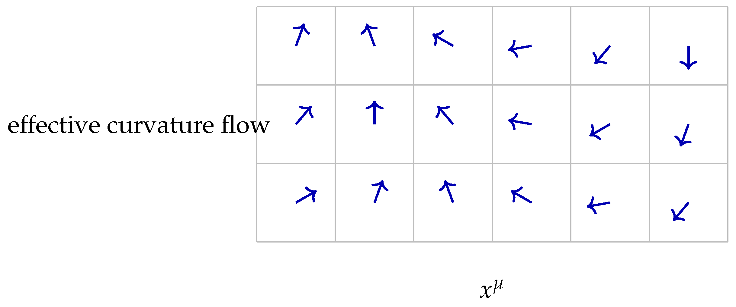
Fluctuations and correlations in the temporal gauge and phase fields distort the effective spacetime grid, producing nontrivial curvature in the emergent geometry, as illustrated schematically in Figure 6.
7.5. Spatial Observables as Euclidean Cross-Sections
Observable space corresponds to a cross-section of the bi-temporal manifold,
equipped with the effective metric
Both temporal domains contribute to , but only through fields and curvatures that survive projection. Temporal curvature, winding numbers, Berry-like phases, and topological charges persist because they depend on generative phase, flux, and topology rather than on manifest temporal orientation.
Consequently, the observed Euclidean three-space can be understood as a stable interface where:
- temporal orientations cancel,
- generative magnitudes combine,
- spatial coordinates align,
- topological structures embed as invariants.
This completes the geometric pathway from dual split-complex Lorentzian domains to the emergent Euclidean geometry of physical space.
8. Discussion
The bi-temporal, split-complex framework developed above provides a concrete geometric mechanism by which an observable Euclidean spatial world and a single effective temporal amplitude can emerge from a deeper dual Lorentzian structure. Each domain is governed by split-complex Lorentzian metrics and independent generative dynamics, yet the observable arena accessible to measurement exhibits neither manifest dual temporal axes nor overt hyperbolic geometry. In this section we examine implications, relations to existing ideas, possible phenomenology, and limitations.
8.1. Bi-Temporal Foundations of Observable Space
The central geometric mechanism is cancellation of conjugate manifest temporal components at the observational interface (Section 2 and Section 3). Concretely,
so that the scalar Euclidean temporal amplitude remains as the physically accessible temporal quantity. Consequently, spatial geometry appears Euclidean to observers not because the fundamental substrate is Euclidean, but because observation projects the two conjugate Lorentzian sectors into a single Euclidean complex plane (cf. Figure 1 and Figure 2).
This geometric viewpoint clarifies two empirical facts simultaneously:
- why we do not detect a reversed temporal orientation in ordinary measurements, and
- why observed spatial relations conform to Euclidean intuition at the level of direct measurement even when underlying generative processes are Lorentzian.
8.2. Relation to Relativistic and Emergent Gravity Pictures
The framework is compatible with relativistic phenomenology while offering a reinterpretation of its origin. The effective metric appearing in Section is not identical to the intrinsic split-complex domain metrics ; rather it is a coarse-grained, dynamical quantity that inherits contributions from temporal phase gradients and temporal curvatures. Accordingly:
- relativistic invariances (local Lorentz-like behavior) can appear as residual symmetries of the split-complex algebra after projection,
- causal structure in the emergent geometry is determined by the alignment of generative flows and the vacuum alignment of the composite order parameter,
- familiar relativistic effects (time dilation, simultaneity relativity) are emergent properties of the effective geometry, not primitive postulates.
8.3. Quantum Phases, Topology, and Phenomenology
Because the temporal gauge connections carry curvature and holonomy, generative dynamics imprint Berry-like phases, flux quantization, and Pontryagin-type charges on the observable sector (Section 6). This leads to several phenomenological suggestions:
- interference phenomena may carry signatures of dual temporal holonomy , in principle observable as phase shifts that cannot be attributed to conventional electromagnetic or geometric phases alone;
- transitions between winding sectors could appear as discrete events or spectral lines in systems sensitive to underlying temporal flux quantization;
- contributions from Pontryagin-like invariants may affect vacuum energy and stability in ways that could be constrained by cosmological observables.
These are speculative but concrete pathways toward empirical access. A detailed phenomenological study is deferred to Section 9, but the logic is clear: topology and holonomy survive Euclidean projection and therefore provide the most robust observational handles on bi-temporal structure.
8.4. Informational and Cognitive Interpretation (Cautionary)
We have modelled the second domain as “informational” (or subjective) to capture internal generative organization without committing to a particular theory of cognition. The formal role of the sector is that of an internal generative substrate that interacts with the objective sector only at the observational interface. This architecture is compatible with, but does not imply, any specific neurobiological or phenomenological theory of mind. We therefore recommend treating cognitive interpretation as a hypothesis supported only by further modelling and empirical constraints, rather than as a consequence of the formalism itself.
8.5. Topological Robustness and Observable Imprints
Topological invariants introduced in Section 6—winding numbers, flux quanta, holonomies, and Pontryagin charges—are insensitive to the sign of manifest time and so persist under Euclidean projection. Therefore they constitute stable, theory-internal labels that can in principle influence observable phenomena (interference, selection rules, vacuum sectors). This robustness makes topology the primary route by which the hidden bi-temporal substrate might be experimentally constrained.
8.6. Limitations, Open Questions, and Future Directions
Several important caveats and open problems remain:
- Derivation of parameters: the coupling constants , the potential parameters , and the scales of generative periods are introduced phenomenologically. Deriving or constraining them from microscopic principles or observations is a priority.
- Backreaction and consistency: when the temporal gauge sectors contribute appreciably to the effective stress tensor, backreaction on the bi-temporal geometry must be analyzed to ensure internal consistency.
- Quantum regime: canonical quantization or path-integral formulation of the coupled gauge–phase system, especially in the presence of topological terms, must be developed to assess quantum stability, anomalies, and possible low-energy effects.
- Operational probes: explicit, realistic experimental setups or astrophysical/cosmological observables that could bound the proposed signatures need to be identified (interferometry, precision spectroscopy, or cosmological correlators are natural starting points).
8.7. Concluding Remarks
The bi-temporal split-complex construction elevates the arrow of time and the Euclidean character of observed space to emergent outcomes of a richer geometric and topological structure. It unifies symmetry-breaking, gauge holonomy, and topological quantization into a single framework that is explicit enough to allow dynamical calculations (Sections –Section 6) and concrete enough to suggest observational tests. We view this framework as a platform: the immediate next steps are a detailed study of quantization and anomaly structure, a focused phenomenological analysis of possible observables, and conservative exploration of cognitive interpretations only once empirical signatures are identified.
9. Phenomenological Outlook
Although the bi-temporal framework is formulated at a fundamental geometric level, it admits several potential phenomenological consequences that, in principle, could be constrained by experiment or observation. The key point is that while manifest temporal components cancel at the Euclidean observational interface, topological and holonomy-based quantities survive (Section 6), making them the most promising carriers of observable signatures.
Interference and geometric-phase effects.
Because each temporal sector supports Berry-like geometric phases arising from temporal holonomy, interference experiments sensitive to phase accumulation may exhibit deviations from standard expectations. Such deviations would not depend on local Lorentzian temporal orientation but on global curvature and flux of the temporal gauge fields. Precision interferometry, atomic clocks, or systems exhibiting topological phase sensitivity provide natural test beds for bounding these effects.
Discrete spectra and winding sectors.
Quantization of temporal curvature flux and winding numbers implies the existence of discrete generative sectors. Transitions between such sectors could manifest as discrete spectral features, selection rules, or stability plateaus in systems sensitive to temporal phase dynamics. While highly model-dependent, this suggests that certain unexplained spectral discretizations or coherence thresholds might admit a geometric interpretation within the bi-temporal framework.
Cosmological and gravitational implications.
At large scales, contributions of temporal gauge curvature and generative phase kinetics to the effective stress–energy tensor (Section ) may influence cosmological evolution. In particular, vacuum contributions associated with Pontryagin-like invariants or symmetry-breaking energy scales could affect early-universe dynamics, cosmic birefringence, or large-scale coherence. Existing cosmological observations therefore place indirect constraints on the allowed parameter ranges of the bi-temporal sector.
Null tests and consistency bounds.
Equally important are null results. The absence of observed violations of Lorentz symmetry, causality, or locality in current experiments strongly constrains any coupling between the bi-temporal structure and low-energy physics. In this sense, the framework is compatible with existing data provided that generative effects enter only through suppressed, topological, or phase-based channels.
Taken together, these considerations suggest that the bi-temporal framework is not immediately falsifiable by a single experiment, but it is constrainable. Its most robust empirical handles lie in topological phases, interference phenomena, and global cosmological observables rather than in local kinematic effects. A detailed phenomenological analysis, including explicit estimates for realistic systems, is left for future work.
10. Conclusion
In this work we have developed a bi-temporal geometric framework in which physical space and observable temporal ordering emerge from the interaction of two orthogonal, split-complex Lorentzian domains. Each domain carries a dual-time structure consisting of a generative temporal coordinate, responsible for the continual reconstruction of spatial or informational configurations, and a manifest temporal coordinate, responsible for sequential ordering. By assigning opposite Lorentzian orientations to the objective and subjective domains, we obtained a pair of conjugate split-complex spacetimes that remain independent at the generative level yet become unified at the moment of observation.
A central result of the framework is that the familiar Euclidean geometry of observable space does not arise as a primitive property of the underlying manifold. Instead, it emerges through a specific cancellation mechanism in which the manifest temporal components of the two domains annihilate at the observational interface,
leaving only a scalar temporal magnitude,
This projection maps the dual split-complex structure into an ordinary complex plane, converting deeper Lorentzian generative dynamics into the Euclidean spatial geometry encountered in physical measurement. Temporal directionality likewise emerges as a consequence of spontaneous breaking of the interchange symmetry between the two domains, encoded in the composite temporal order parameter .
Introducing independent temporal gauge connections and phase fields allowed the theory to be formulated in a gauge-covariant manner. Their associated curvatures generate geometric and topological phenomena, including Berry-like phases, flux quantization, and Pontryagin-type invariants. Crucially, these quantities survive the Euclidean projection and therefore provide potential observational handles on the deeper bi-temporal structure. The Einstein-like equations derived from the action further show that the curvature of observed spacetime can be interpreted as emerging from generative temporal dynamics rather than being imposed as a fundamental background.
Beyond its geometric and dynamical content, the bi-temporal framework offers a unified perspective on physical and informational processes. The subjective domain—absent from conventional spacetime models—is incorporated as a conjugate Lorentzian sector whose generative and manifest times interact with the objective domain only through the Euclidean observational interface. While no specific theory of cognition is implied, the formal structure naturally accommodates internal generative organization alongside physical dynamics within a single geometric architecture.
Several directions for future research follow naturally:
- Relativistic and cosmological dynamics. The influence of bi-temporal curvature and symmetry breaking on cosmological evolution, gravitational waves, and causal structure warrants detailed investigation, particularly regarding possible early-universe imprints.
- Quantum phases and interference. Temporal holonomy and flux quantization suggest experimental searches in precision interferometry and systems exhibiting topological order.
- Mathematical development. The geometry of split-complex fiber bundles with dual gauge connections presents a rich mathematical structure, especially in relation to moduli spaces and topological classification.
- Phenomenological constraints. Explicit models connecting the bi-temporal sector to observable quantities are needed to assess empirical viability and establish bounds on the theory’s parameters.
- Unification perspectives. By integrating geometry, gauge theory, and topology within a single temporal architecture, the framework may offer new tools for bridging classical and quantum descriptions of spacetime.
In summary, the bi-temporal split-complex formulation provides a coherent and geometrically natural account of how Euclidean space, temporal directionality, gauge structure, and topological quantization can emerge from a deeper temporal substrate. By treating observation as an intrinsic geometric process rather than an external assumption, the framework suggests a broader view of physical law in which spacetime structure, dynamical evolution, and informational organization arise from the same underlying generative dynamics.
Appendix A Split-Complex Algebra and Geometry
The bi-temporal framework introduced in this paper relies fundamentally on the algebra of split-complex numbers, also known as hyperbolic, Lorentz, or duplex numbers. This appendix summarizes the essential algebraic and geometric properties of the split-complex system used throughout the manuscript.
Appendix A.1. Definition and Basic Properties
A split-complex number is an ordered pair with algebraic representation
where j is a hyperbolic unit satisfying
This contrasts with the ordinary complex unit i, which satisfies .
Addition and multiplication follow:
The split-complex conjugate is defined by
Appendix A.2. Norm and Lorentzian Signature
Unlike ordinary complex numbers, the split-complex norm is indefinite:
This norm has a Minkowski-like signature and endows the space of split-complex numbers with a natural Lorentzian geometry.
Thus, the split-complex plane
is isomorphic to 1+1 Lorentzian spacetime, with:
- x interpreted as a spatial coordinate,
- t interpreted as a Lorentzian temporal coordinate.
The “lightlike’’ elements satisfy , giving the null lines .
Appendix A.3. Hyperbolic Rotations (Lorentz Boosts)
Multiplication by generates hyperbolic rotations:
giving the transformation
Explicitly,
These are precisely Lorentz boosts in 1+1 dimensions.
Thus, the linear symmetry group of the split-complex plane is isomorphic to .
Appendix A.4. Split-Complex Coordinates and Metrics
For each temporal domain we introduced the split-complex coordinate
Its differential satisfies
yielding the natural metric
with the additional generative coordinate included as a fiber direction of positive norm.
The subjective domain is assigned the conjugate signature
reflecting its reversal of temporal orientation.
Appendix A.5. Tensor Products and Bi-Temporal Geometry
The full bi-temporal manifold employs two split-complex planes:
Their direct sum
is equipped with a metric of signature , corresponding to the objective and subjective domains, respectively. Orthogonality of the two Lorentzian sectors ensures that their contributions remain distinct until projected into the Euclidean observational interface.
Appendix A.6. Split-Complex vs. Ordinary Complex Structure
The Euclidean observational coordinate
arises from a projection that replaces the hyperbolic unit j with the imaginary unit i after cancellation of the manifest temporal components. Thus:
- Split-complex algebra governs the deeper generative structure of spacetime.
- The ordinary complex algebra governs the observable Euclidean structure.
This transition is a geometric manifestation of the cancellation
and the preservation of generative magnitude
Appendix A.7. Relevance to Temporal Geometry and Gauge Structure
The split-complex algebra is essential for representing:
- Lorentzian signatures in each domain,
- hyperbolic rotations as intrinsic temporal transformations,
- the natural coupling between generative and manifest time levels,
- the dual gauge structure expressed through temporal connections ,
- the symmetry-breaking mechanism exchanging the two domains,
- the Euclidean emergence resulting from temporal cancellation.
Thus, the split-complex foundation is not an auxiliary mathematical choice but the geometric backbone of the entire bi-temporal theory.
Appendix B Gauge Invariants and Topological Quantities
The bi-temporal framework possesses a rich collection of gauge-invariant and topological structures arising from the temporal connections and their curvatures . These invariants remain well-defined even after the Euclidean projection of the observable world, as they depend on flux, holonomy, and winding rather than on the Lorentzian orientation of the temporal axes. This appendix summarizes the principal invariants used throughout the manuscript.
Appendix B.1. Temporal Gauge Transformations
Each domain carries an independent -like temporal gauge symmetry:
under which the covariant derivative and curvature transform as:
Thus, both and are gauge-invariant.
Appendix B.2. Fundamental Quadratic Invariants
The simplest gauge-invariant scalars for each domain are:
- Interpretation.
- measures the strength of temporal curvature.
- measures the generative temporal flow in each domain.
These invariants appear both in the action functional and in the energy–momentum tensor, playing roles analogous to electromagnetic and scalar kinetic invariants.
Appendix B.3. Cross-Domain Composite Invariants
Cross-domain invariants are constructed to preserve the temporal interchange symmetry:
This composite field acts as the symmetry-breaking order parameter and encodes the combined generative activity of both domains.
Higher-order invariants include:
which couple the two temporal sectors and appear in generalized interaction terms.
Appendix B.4. Temporal Flux Quantization
Integrating the curvature two-form over a closed 2-surface yields the temporal flux:
Single-valuedness of the temporal phase fields around closed loops implies quantization:
Thus each domain admits its own set of quantized flux sectors:
which survive Euclidean projection and affect observable interference phenomena.
Appendix B.5. Holonomy and Berry-like Geometric Phases
For a closed loop C in , the temporal holonomy is:
Using Stokes’ theorem:
- Interpretation.
- is a Berry-like phase associated with generative time.
- It determines interference patterns in fields sensitive to .
- These phases persist under Euclidean projection since they depend on flux, not on the orientation of manifest time.
Appendix B.6. Winding Numbers and Generative Cycles
Inner-time dynamics may contain closed generative cycles:
with integer winding numbers
These correspond to elements of the fundamental group
Thus, the generative sectors possess two independent homotopy integers
These topological invariants classify generative histories and are unaffected by the manifest-time cancellation at the observational interface.
Appendix B.7. Pontryagin-like Topological Densities
Each curvature defines a Pontryagin-type pseudoscalar:
The corresponding topological charges are:
These invariants classify nontrivial sectors of the temporal gauge fields, analogous to instantons or Chern–Simons configurations.
They remain invariant under:
- gauge transformations,
- smooth deformations of the fields,
- Euclidean observational projection.
Appendix B.8. Summary of Invariants
The complete set of independent gauge and topological invariants in the bi-temporal framework includes:
These invariants form the backbone of the dual temporal gauge structure and encode all global information that persists through the Euclidean emergence of observable space.
Appendix C Extended Derivations
In this appendix we present the detailed derivations of the field equations obtained from the action functional introduced in Section E, and clarify the underlying symmetry structure. We adopt the convention that indices are raised and lowered using the effective metric unless otherwise specified.
Appendix C.1. Variation with Respect to the Temporal Gauge Fields
Recall the bi-temporal action
We first vary S with respect to . The -sector curvature is
and its variation obeys
since the Levi-Civita connection is torsion-free and metric-compatible.
- Curvature term.
The variation of the kinetic term for is
Substituting and integrating by parts gives
where a boundary term has been discarded.
- Phase-kinetic term.
The -sector kinetic term for is
The variation with respect to arises from
Hence,
- θ ˜-term.
The topological term varies as
An integration by parts shows that this contribution is a total derivative in the absence of spacetime boundaries or when is constant, so it does not modify the local equations of motion.
- Result.
Combining the above variations and demanding yields
which is the field equation quoted in Section E. An analogous derivation holds for the sector with the replacements .
Appendix C.2. Variation with Respect to the Temporal Phase Fields
We now vary the action with respect to . Only the kinetic term and the potential contribute.
- Kinetic term.
The variation of with respect to is
with
since the variation is handled separately. Integrating by parts yields
- Potential term.
The potential depends on , which in turn depends on . Thus
- Result.
Setting gives
The corresponding equation for is obtained by .
Appendix C.3. Variation with Respect to the Metric
Finally, we vary the action with respect to the effective metric . The Einstein–Hilbert term yields the standard result
where is the Einstein tensor.
- Curvature terms.
The curvature contributions from the gauge fields are
Their variation with respect to gives the stress–energy contributions
- APhase-kinetic terms.
The phase contributions read
Varying with respect to gives the stress–energy tensors
- Potential term.
The potential contributes
so that the corresponding stress–energy contribution is simply
- Result.
Collecting all pieces and setting yields
which is the modified Einstein equation quoted in Section E.
Appendix C.4. Symmetry Algebra: Gauge and Interchange Symmetries
The full symmetry algebra of the bi-temporal theory consists of:
-
Gauge symmetries acting independently in each domain:These symmetries leave and invariant.
-
Temporal interchange symmetry exchanging the two domains:This symmetry acts as an involution,and leaves the composite order parameter and the potential invariant.
Before symmetry breaking, the total symmetry group is
where the semidirect product encodes the fact that exchanges the two factors. Spontaneous symmetry breaking selects a preferred vacuum expectation value for , reducing the symmetry and generating the observed arrow of time.
This completes the derivation of the field equations and the characterization of the symmetry structure for the bi-temporal split-complex framework.
Appendix D Summary of Notation
This appendix summarizes the principal symbols and conventions used throughout the manuscript. Symbols are grouped according to their roles in the bi-temporal split-complex framework.
Coordinates and Temporal Variables
| Symbol | Meaning |
| Spatial coordinates in the objective or subjective domain, . | |
| Manifest temporal coordinates with opposite Lorentzian orientations . | |
| Generative (inner) temporal coordinates in each domain. | |
| Split-complex coordinate for each domain, . | |
| Extended split-complex coordinate including generative time. | |
| O | Euclidean temporal magnitude: . |
| Effective Euclidean complex coordinate after observation. |
Manifolds and Domains
| Symbol | Meaning |
| Objective split-complex Lorentzian domain with orientation . | |
| Subjective split-complex Lorentzian domain with orientation . | |
| Generative-time fibers associated with each domain. | |
| Bi-fibered temporal manifold: . | |
| Euclidean observational interface where . |
Split-Complex Geometry
| Symbol | Meaning |
| j | Hyperbolic unit, . |
| Split-complex norm with Lorentzian signature. | |
| Metrics of the objective and subjective domains. | |
| Inverse metrics on . | |
| Effective emergent spacetime metric after projection. | |
| Hyperbolic rotation (Lorentz boost) of rapidity . |
Temporal Gauge Fields and Curvatures
| Symbol | Meaning |
| Temporal gauge connections in each domain. | |
| Temporal curvature tensors: . | |
| Gauge couplings for and temporal sectors. | |
| Levi-Civita covariant derivative associated with . |
Phase Fields and Symmetry Breaking
| Symbol | Meaning |
| Temporal phase fields in each domain. | |
| Covariant derivatives: . | |
| Composite order parameter controlling symmetry breaking. | |
| Symmetry-breaking potential with degenerate minima. | |
| Temporal interchange symmetry exchanging and domains. |
Topological Invariants
| Symbol | Meaning |
| Winding numbers of generative cycles . | |
| Quantized temporal flux through a surface . | |
| Berry-like geometric phase along a closed curve C. | |
| Pontryagin density: . | |
| Topological charges associated with . | |
| Scalar invariants formed from curvatures and phase gradients. |
Action and Dynamical Quantities
| Symbol | Meaning |
| S | Total action of the bi-temporal system. |
| R | Ricci scalar of the effective geometry. |
| Einstein tensor associated with . | |
| Gravitational coupling constant. | |
| Coefficients of temporal curvature terms. | |
| Strength of generative phase kinetics. | |
| Coefficients of topological -terms. |
Projection and Observational Quantities
| Symbol | Meaning |
| Observed manifest time (vanishes at the Euclidean interface). | |
| O | Observable scalar temporal magnitude after projection. |
| Euclidean spatial slice accessible to measurement. | |
| Euclidean complex coordinate representing observed space-time events. |
Constants and Conventions
| Symbol | Meaning |
| Euclidean spatial metric on . | |
| Totally antisymmetric Levi-Civita tensor density. | |
| Temporal orientations of the Lorentzian domains. | |
| Natural units adopted unless otherwise specified. |
This notation summary provides a comprehensive reference for all mathematical structures appearing in the dual split-complex temporal framework.
References
- Heisenberg, W. Physics and Philosophy: The Revolution in Modern Science; Harper and Row, 1958. [Google Scholar]
- Nambu, Y. Quasi-Particles and Gauge Invariance in the Theory of Superconductivity. Physical Review 1960, 117, 648–663. [Google Scholar] [CrossRef]
- Goldstone, J. Field Theories with Superconductor Solutions. Il Nuovo Cimento 1961, 19, 154–164. [Google Scholar] [CrossRef]
- Einstein, A. Die Feldgleichungen der Gravitation. Sitzungsberichte der Preussischen Akademie der Wissenschaften 1915, 844–847. [Google Scholar]
- Cartan, E. Sur les variétés à connexion affine et la théorie de la relativité générale. Annales scientifiques de l’École Normale Supérieure 1925, 42, 17–88. [Google Scholar] [CrossRef]
- Weyl, H. Gravitation und Elektrizität. Sitzungsberichte der Preussischen Akademie der Wissenschaften 1918, 465–480. [Google Scholar]
- Yang, C.N.; Mills, R.L. Conservation of Isotopic Spin and Isotopic Gauge Invariance. Phys. Rev. 1954, 96, 191–195. [Google Scholar] [CrossRef]
- Witten, E. Topological Quantum Field Theory. Communications in Mathematical Physics 1988, 117, 353–386. [Google Scholar] [CrossRef]
- Witten, E. Quantum Field Theory and the Jones Polynomial. Communications in Mathematical Physics 1989, 121, 351–399. [Google Scholar] [CrossRef]
- Rovelli, C. Time in quantum gravity: An hypothesis. Physical Review D 1991, 43, 442–456. [Google Scholar] [CrossRef] [PubMed]
- Barbour, J. The End of Time; Oxford University Press, 1999. [Google Scholar]
- Kuchař, K. Time and interpretations of quantum gravity. In Proceedings of the Proceedings of the 4th Canadian Conference on General Relativity and Relativistic Astrophysics, Singapore, 1980; pp. 211–314. [Google Scholar]
- Misner, C.W.; Thorne, K.S.; Wheeler, J.A. Gravitation; W. H. Freeman and Co.: San Francisco, 1973. [Google Scholar]
- Aharonov, Y.; Anandan, J. Phase change during a cyclic quantum evolution. Physical Review Letters 1987, 58, 1593–1596. [Google Scholar] [CrossRef] [PubMed]
- Carollo, A.; Vedral, V. Berry phase in quantum information processing. Physical Review Letters 2003, 90, 157903. [Google Scholar]
- Boi, L. Symmetry and Symmetry Breaking in Physics: From Geometry to Topology. Symmetry 2021, 13, 2100. [Google Scholar] [CrossRef]
- Haj Yousef, M.A. The concept of time in Ibn Arabi’s cosmology and its implication for modern physics. Ph.D. thesis, 2007 as (Ibn Arabi - Time and Cosmology). University of Exeter, Exeter, UK, Routledge, 2005. [Google Scholar]
- Haj Yousef, M.A. Ibn Arabi – Time and Cosmology; Routledge: London, New York, 2007. [Google Scholar]
- Haj Yousef, M.A. The Single Monad Model of the Cosmos: Ibn Arabi’s Concept of Time and Creation; CreateSpace: Charleston, 2014. [Google Scholar]
- Haj Yousef, M.A. DUALITY OF TIME: Complex-Time Geometry and Perpetual Creation of Space; The Single Monad Model of The Cosmos, Book 2; CreateSpace: Charleston, 2017. [Google Scholar]
- Haj Yousef, M.A. ULTIMATE SYMMETRY: Fractal Complex-Time, the Incorporeal World and Quantum Gravity.
- Haj Yousef, M.A. Zeno’s Paradoxes and the Reality of Motion According to Ibn al-Arabi’s Single Monad Model of the Cosmos. In Islamic and Christian Philosophies of Time, Vernon Series in Philosophy; Mitralexis, S., Ed.; Vernon Press: Wilmington, USA, 2018; Volume chapter 7, pp. 147–178. [Google Scholar]
- Kobayashi, S.; Nomizu, K. Foundations of Differential Geometry; Wiley, 1963; Vol. 1. [Google Scholar]
- Nakahara, M. Geometry, Topology and Physics, 2nd edition; Taylor & Francis / CRC Press, 2003. [Google Scholar]
- Higgs, P.W. Broken Symmetries and the Masses of Gauge Bosons. Physical Review Letters 1964, 13, 508–509. [Google Scholar] [CrossRef]
- Landau, L.D. On the Theory of Phase Transitions. In Zh. Eksp. Teor. Fiz.;English translation: Collected Papers of L. D. Landau; Pergamon Press, 1937; Volume 7, pp. 19–32. [Google Scholar]
- Kibble, T.W.B. Topology of Cosmic Domains and Strings. Journal of Physics A: Mathematical and General 1976, 9, 1387–1398. [Google Scholar] [CrossRef]
- Berry, M.V. Quantal phase factors accompanying adiabatic changes. Proceedings of the Royal Society A 1984, 392, 45–57. [Google Scholar] [CrossRef]
- Dirac, P.A.M. Quantised Singularities in the Electromagnetic Field. Proceedings of the Royal Society A 1931, 133, 60–72. [Google Scholar] [CrossRef]
- Simon, B. Holonomy, the quantum adiabatic theorem, and Berry’s phase. Physical Review Letters 1983, 51, 2167–2170. [Google Scholar] [CrossRef]
- Jackiw, R. Topological Investigations of Quantized Gauge Theories. Current Algebra and Anomalies Reprinted collection; see references therein. 1985, 211–359. [Google Scholar]
- Verlinde, E. On the Origin of Gravity and the Laws of Newton. Journal of High Energy Physics 2011, 2011, 029. [Google Scholar] [CrossRef]
Figure 1.
Conceptual illustration of the observation map . The inner generative time and outer physical time t define Lorentzian temporal sectors associated with subjective and objective domains. Observable events arise at their Euclidean intersection, represented as the effective interface of measurement and perception.
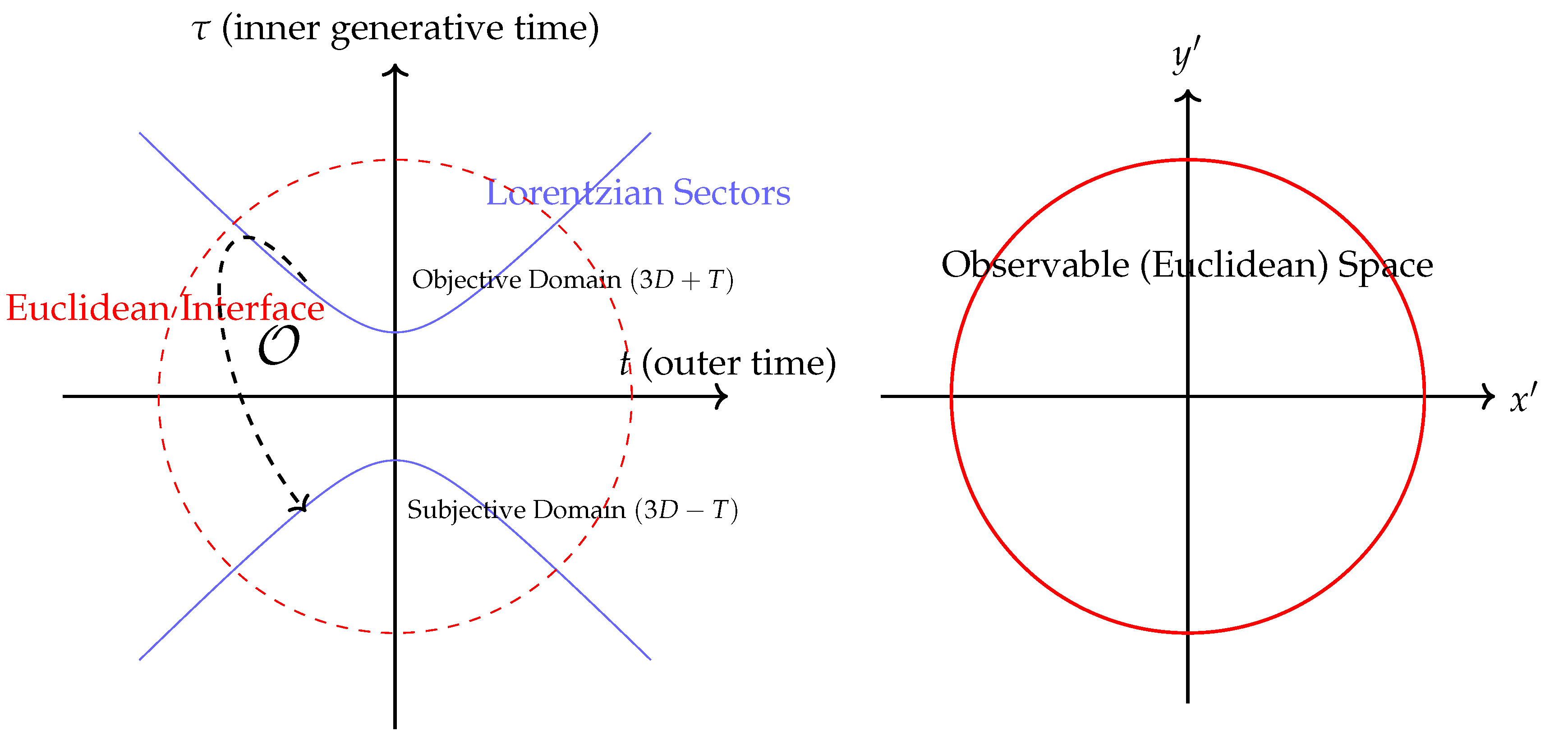
Figure 2.
Dual-time manifold representation. Interaction between the temporal coordinates generates a Euclidean projection (dashed circle) representing observable time. Symmetry breaking distinguishes t from , producing temporal orientation.
Figure 2.
Dual-time manifold representation. Interaction between the temporal coordinates generates a Euclidean projection (dashed circle) representing observable time. Symmetry breaking distinguishes t from , producing temporal orientation.
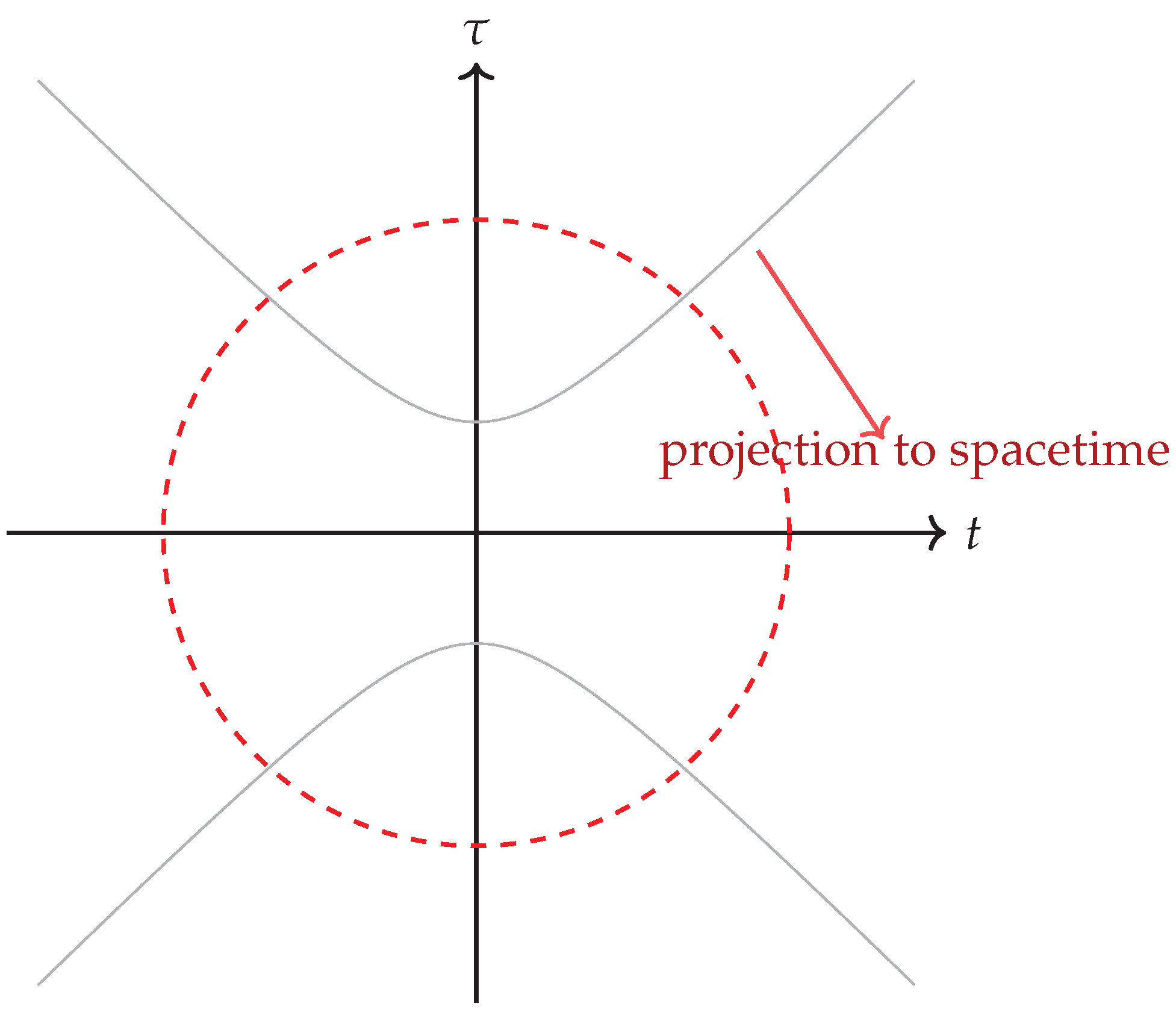
Figure 3.
Berry-like phase as an observable arising from the temporal connection. The integrated curvature over a surface bounding determines the geometric phase.
Figure 3.
Berry-like phase as an observable arising from the temporal connection. The integrated curvature over a surface bounding determines the geometric phase.
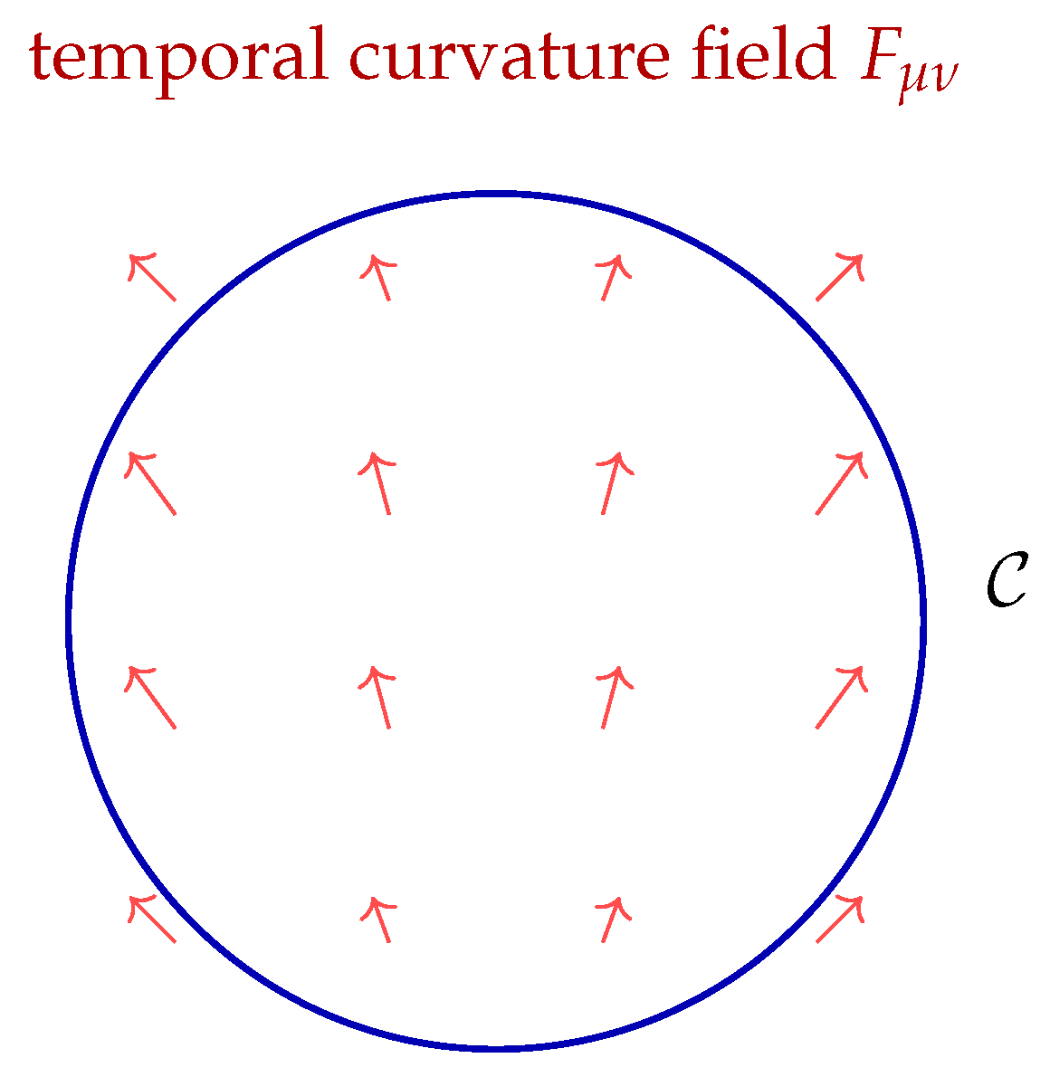
Figure 4.
Topological quantization of inner-time evolution: closed loops in the generative coordinate form winding sectors labeled by an integer n, each corresponding to a discrete contribution to an action or phase.
Figure 4.
Topological quantization of inner-time evolution: closed loops in the generative coordinate form winding sectors labeled by an integer n, each corresponding to a discrete contribution to an action or phase.
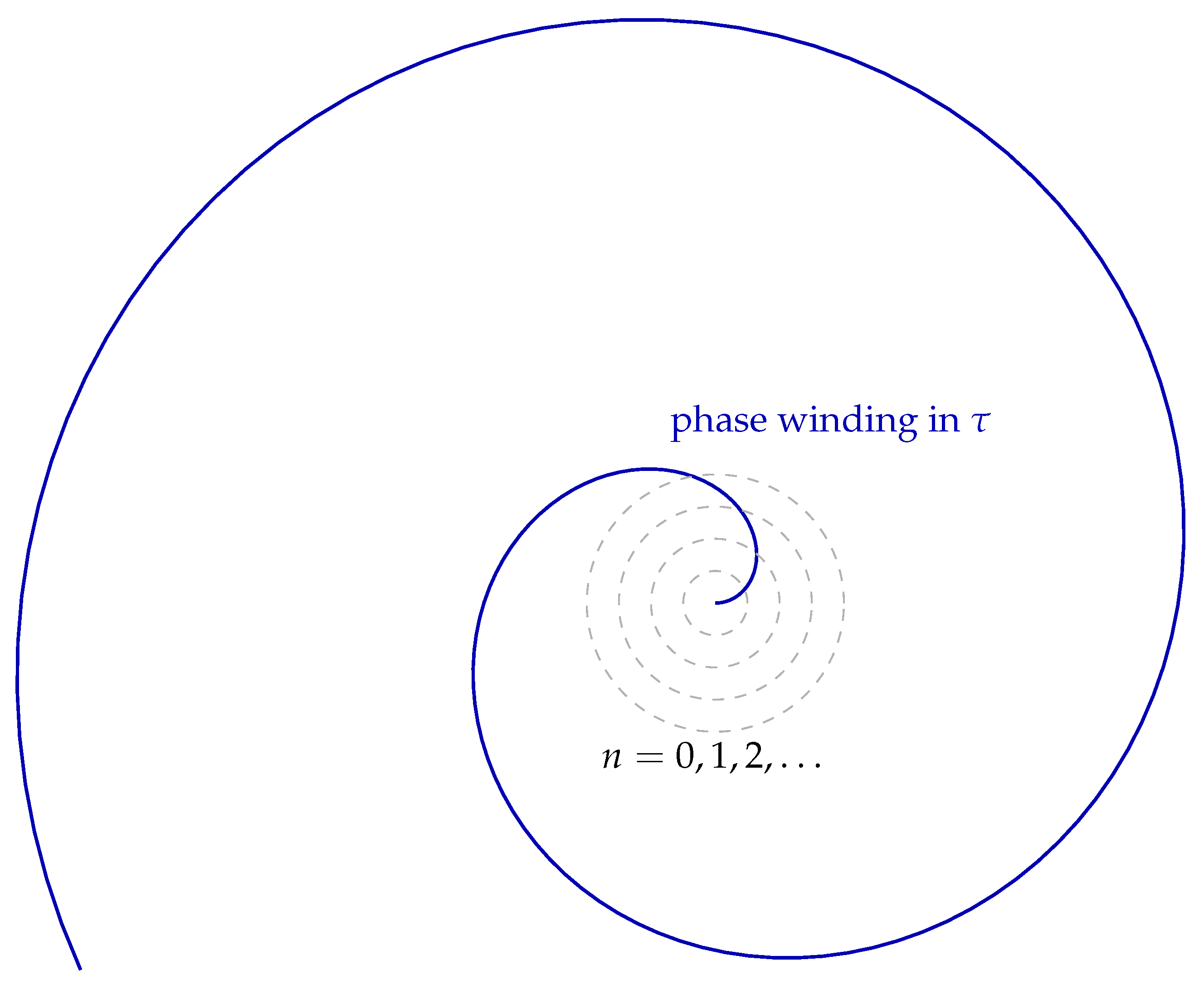
Figure 5.
Topological structure of dual-time evolution: closed loops in the inner-time coordinate represent generative cycles, while open trajectories in the outer time t represent the observable progression of physical processes. The interplay of these structures supports discrete temporal sectors.
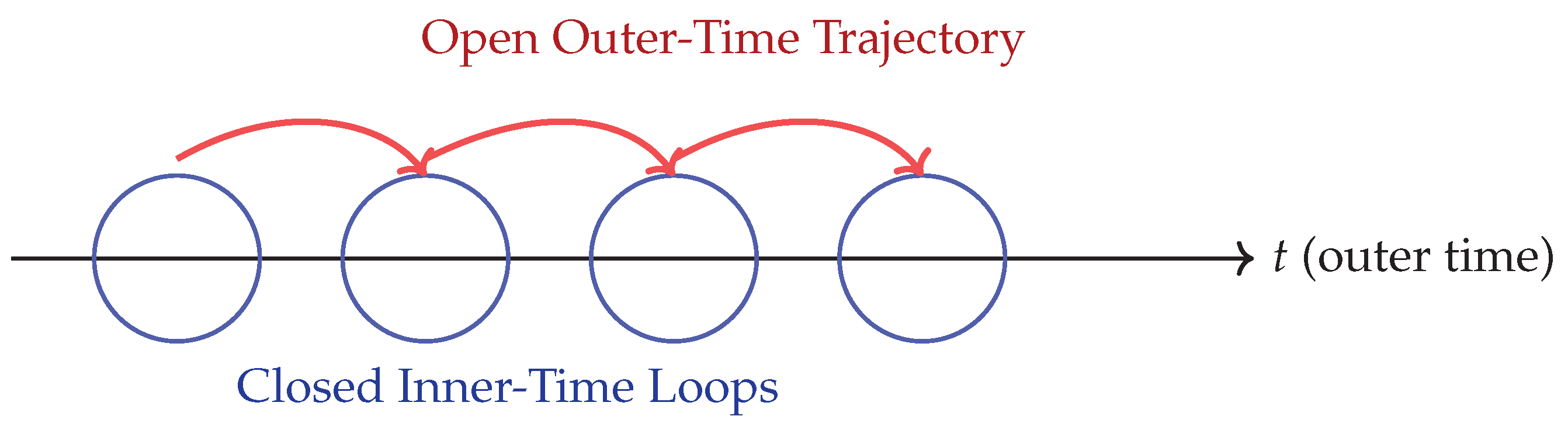
Figure 6.
Illustration of emergent curvature: fluctuations and correlations in the temporal gauge and phase fields distort the effective spacetime grid, producing a nontrivial Ricci tensor as expressed in Eq. ().
Figure 6.
Illustration of emergent curvature: fluctuations and correlations in the temporal gauge and phase fields distort the effective spacetime grid, producing a nontrivial Ricci tensor as expressed in Eq. ().
Disclaimer/Publisher’s Note: The statements, opinions and data contained in all publications are solely those of the individual author(s) and contributor(s) and not of MDPI and/or the editor(s). MDPI and/or the editor(s) disclaim responsibility for any injury to people or property resulting from any ideas, methods, instructions or products referred to in the content. |
© 2025 by the authors. Licensee MDPI, Basel, Switzerland. This article is an open access article distributed under the terms and conditions of the Creative Commons Attribution (CC BY) license (http://creativecommons.org/licenses/by/4.0/).
Copyright: This open access article is published under a Creative Commons CC BY 4.0 license, which permit the free download, distribution, and reuse, provided that the author and preprint are cited in any reuse.


