
Submitted:
15 November 2025
Posted:
17 November 2025
You are already at the latest version
Abstract
The concept of Geometric Phase in Quantum Mechanics is generally formulated en- tirely in terms of geometric structure of complex Hilbert Space. This tutorial article gives a general mathematical overview of the Geometric phase introduced by Berry with the conditions over the system’s evolution embedded through adiabaticity and cyclicity, which were subsequently relaxed sequentially by Aharonov-Anandan, Samuel-Bhandari, and later by Mukunda and Simon by using the idea of Bargmann Invariants. The arti- cle presents a thorough and illustrative overview regarding the mathematical derivation behind the upliftment of the conditions, which results in the generalized definition of the Geometric phase for quantum systems. In addition to that, the article also gives an overall idea about the general analytical aspects of finding the Geometric phase for three level open quantum systems undergoing decoherence and dephasing due to interaction with the surroundings in the weak system reservoir coupling limit described by quantum master equations.
Keywords:
berry phase
; Aharonov Anandan phase
; Bargmann invariants
; Lindblad master equation
; mixed states
1. Introduction
A Pure Quantum State retains a memory of its evolution in terms of Geometric Phase when it undergoes an evolution in the Parameter Space.The phase factor has its origin which is purely geometric in nature and it can arise even under the most general conditions where the system is undergoing an non-unitary evolution corresponding to the Hamiltonian which does not satisfy the criterion of adiabaticity and cyclicity. Although when geometric phase comes into the picture we talk about Berry’s framework [4] where he assumed the evolution to be cyclic in the parameter space and the Hamiltonian’s obeys the adiabeticity and cyclicity condition but Pancharatnam’s experimental work [9] on interference in 1956 gives us the idea about the existence of such phase factor which is known as pancharatnam connection which states that if we consider any three mutually nonorthogonal vectors in a certain hilbert space say so that, then if is in phase with and is in phase with then may not be in phase with .The relative phase difference between any two non-orthogonal vectors is defined as follows.
Let us consider two vectors and such that they have a non zero value of inner product which is in general complex i.e. and any complex number can be represented in the polar coordinate so with and here denotes the relative phase difference between the vectors. Now in Pancharatnams[5]framework the three vectors were the three different electric fields E1,E2,E3 say so that chosen for the interferrometry experiment and experimentally the Pancharatnams[14] connection was found with the fact that when the two electric fields are in phase with each other it will correspond to the interference maximum and when the relative phase difference between them be it will correspond to the minimum in the interference pattern i.e. the intensities will be maximum and minimum when they are in phase or out of phase. Apparently there is no quantum mechanics or Schrodinger equation [24] is involved in the Pancharatnams [11,12] framework as it comes form the result of experimental classical optics but it has a connection in the Three dimensional Poincare sphere representation of the manifold.
But after Berry’s discovery of the geometric phase enormous amount of work has been done to generalize the idea of the geometric phase and Aharonov and Anandan [1] showed that if we lift up the condition of adiabaticity still one can define the geometric phase and the total phase can be written as a sum of the geometric phase and dynamical phase keeping the condition of cyclical evolution [18] of the quantum system and the geometric phase in their framework is called Aharonov-Anandan Phase.
After Aharonov Anandan’s discovery Samuel and Bhandari [23] further relaxed the condition of the cyclicity as the condition of adiabaticity has already been lifted in Aharonov-Anandans framework and gives the definition of the geometric phase for the non cyclic and non adiabatic evolution of the quantum system.All the approaches of the generalization of the Geometric phase requires the time dependent Schrodinger equation so these are known as the dynamic approach but Mukunda and simon [19] defined the geometric phase from the kinematic point of view which does not require the schrodinger equation hence the evolution of the quantum system can be non-unitary, thereby proving that the geometric phase is a Ray space quantity and showed that for three arbitrary non-orthogonal state vectors the non-vanishing geometric phase is given by the Bargmann Invariant of order 3 abbreviated by BI(3) [22]. Hence, with are the pure state density matrices corresponding to the states and by definition of the density or projection operators we have and .So far all the calculations on the geometric phase has been done for the pure states now it can be generalized for the mixed states too. In the present context we try to find out an expression of the Geometric phase for a three level open quantum system by the SU(3) representations [13] using the fact that the mixed states lie on the interior of the eight dimensional Bloch sphere.
In the first part of this tutorial we present the idea of the Geometric phase introduced by Michael Berry imposing the conditions of adiabaticity and cyclicity to describe the evolution of the system in the parameter space and how the conditions of the adiabaticity and cyclicity was eventually uplifted by Aharonov-Anandan and later by Samuel-Bhandarai and Mukunda-Simon. In the later part of this article we present a brief overview for the calculation of geometric phase for three level open quantum system undergoing a non-unitary evolution with its dynamics described by the Lindblad master equation[16] along with the insights of master equations. In the last section we gave the mathematical derivation for the calculation of geometric phase for mixed states undergoing non unitary evolution.
Previously progress has been made on the calculation of the geometric phases for two level open quantum systems and there are works on geometric phases for mixed states using the Schmidt’s purification method which lifts the mixed states to pure states. Geometric phase for the three level quantum system of the mixed states can be defined by establishing in connecting the density matrix with the non-unit vector ray in a three dimensional complex Hilbert space. Because the Geometric Phase depends only on the smooth curve on this space,it is formulated entirely in terms of geometric structures.Under the limiting of pure state,the approach is in agreement with the Berry’s phase, Pancharatnam phase and Aharonov and Anandan Phase.We observe that Berry phase of mixed state correlated to population inversions of three level open quantum system devised by Jiang et al [13].
2. Review of Previous works related to Geometric Phases
2.1. Berry’ Discovery of Geometric Phase
A Pure Quantum State retains a memory of its evolution in terms of Geometric Phase when it undergoes a closed evolution in the Parameter Space, where the Geometric Phase essentially arises as an effect of Parallel Transport in the Poincare Representation of the manifold.Berry first pointed out the existence of such phase under the condition of adiabaticity,cyclicity and the unitary evolution of the quantum system i.e. if the System is characterized by some time dependent Hamiltonian having a non-degenerate energy eigenvalue spectrum (assuming no level crossing between two energy levels) and it undergoes a cyclic and unitary evolution then the time dependent Energy eigenvalues will also obey the cyclic condition. If the system is characterized by the Hamiltonian which is cyclic i.e for some , then the energy eigenvalues which forms a non-degenerate spectrum will also obey the cyclicity condition i.e. for some .Naturally one can ask whether the eigenfunctions of the Hamiltonian denoted by so that, will satisfy the similar condition of cyclicity? The answer is no, now comes the idea of the Geometric phase.The most general solution of the Time Dependent Schrodinger equation satisfies the following condition as a result of the Adiabatic Approximation Theorem given by, and the time evolution of the state vector is governed by the time dependent Schrodinger’s equation given by,
they get connected by the total phase factor along with the eigenstates of the Hamiltonian will obey the following condition:
where, the total phase factor can be written as the sum of the dynamical phase and the geometric phase and using the adiabatic approximation theorem one can show that if the Hamiltonian of the quantum system is slowly varying with time then if the system starts initially in the nth eigenstate of the Hamiltonian then it will remain in the nth eigenstate of it just by picking a couple of phase factor the former being the usual dynamical phase and the later being the Geometric phase. We can write,
where, and .
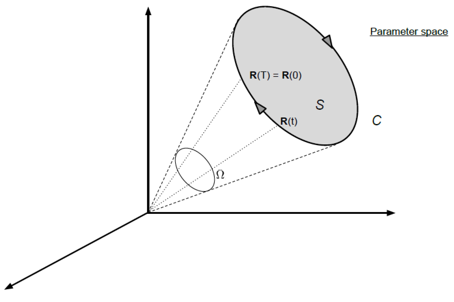
In Berry’s framework the Hamiltonian is a function of some parameters defined in the parameter space and the dimensionality of the Parameter space being equal to the number of parameters and the Hamiltonian obeys the cyclicity condition which is incorporated in the original derivation by considering a closed curve in the parameter space.We define the closed curve in the parameter space such that for some and the geometric phase in berry’s framework can be expressed as a closed integral over the multidimensional parameter space and it is given by,. Now exploiting the completeness relation of the normalized eigenstates of the Hamiltonian we can write,
Where, and now if we consider a 3 dimensional parameter space then the above line integral in equation(4) can be converted into a surface integral using the stokes theorem of curl and it leads to,
here the completeness relation of the eigenstates of the Hamiltonian i.e. has been used in the second step.Simplification of equation(5) leads to the final expression of the Geometric Phase and it turns out to be where be the solid angle subs tended by the closed curve in the parameter space at origin and it is apparent that the geometric phase only depends on the nature of the closed curve in the parameter space and hence independent of the nature of the quantum system and the general feature of the geometric phase has been reflected in Berry’s framework.
Figure 1.
Closed curve C in the parameter space R.
2.2. Aharonov’s Aharonov Phase and a Generalization
The next work is Aharonov-Anandan’s Generalisation which shows that the total phase can be written as the sum of the dynamical phase and the geometric phase if we lift up the condition of adiabaticity and allow the system to have a cyclic evolution but here the condition of the cyclicity has been imposed through the notion of the ray space or projective Hilbert Space denoted by where the pure state density operator or the projection operator obeys the condition of cyclicity in the projective Hilbert space described by a closed path or trajectory in . Let the Hamiltonian of the system be and any arbitrary state vector whose evolution is governed by the time dependent schrodinger equation given by,
The solution of the above equation requires the initial condition i.e. and the solution of the time dependent Schrodinger equation defines a smooth curve in ,the idea is to associate a each point of the state space for different and it will define a smooth parametrized curve in the state space such that for every there is a at each point of the curve. Now if we considering a mapping between the State space and the projective Hilbert space i.e. so that every single point on the curve C is being mapped to their corresponding density operators i.e. ; those points defines an image curve in the projective Hilbert space.The time evolution of the density operator is governed by the Von-Neumann Louiville equation in the Projective Hilbert space given by,
there is no assumption regarding the adiabaticity of the hamiltoinian but here we will consider cyclic evolution of the quantum system described by the closed trajectory or a closed parametrized curve The above condition will held if and differ from each other up-to a phase factor so that we can write, the phase factor by which the state vectors at time and differs is called the total phase in Aharonov Anandans framework[15].Later Aharonov and Anandan showed that the total phase can be written as the sum of the dynamical phase and the Geometric phase or Aharonov-Anandan phase.The expressions for the phases are as follows,
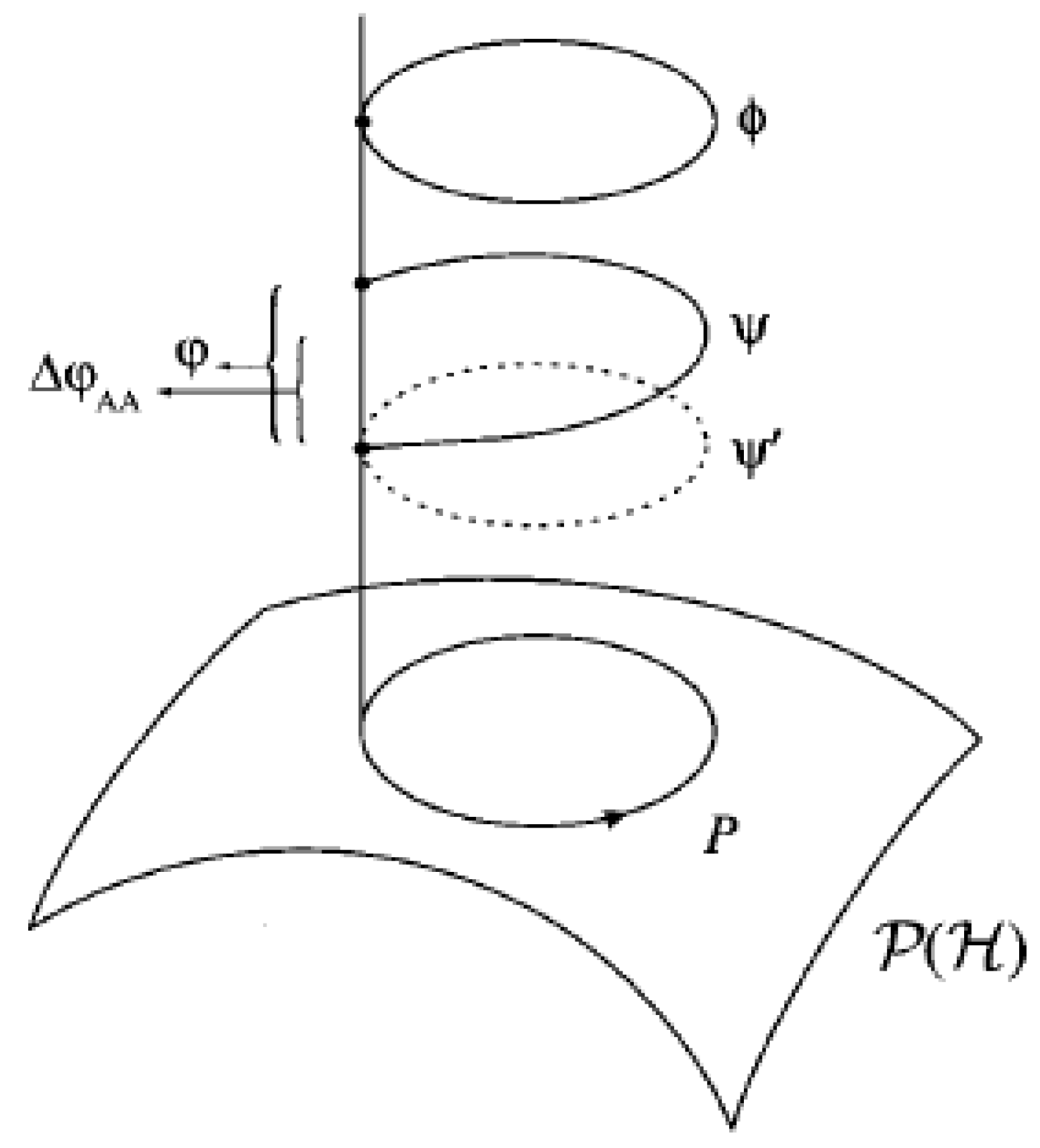
Let, be an arbitrary closed curve in projecting onto so that (as shown in the figure below) and differs by a phase factor i.e. along with because of cyclicity and after a little bit of simplification we get;
Figure 2.
Three different lifts of the curve P in :-solution of original schrodinger equation; the solution of the schrodinger equation corresponding to the transformed hamiltonian and -an arbitrary closed curve.
Figure 2.
Three different lifts of the curve P in :-solution of original schrodinger equation; the solution of the schrodinger equation corresponding to the transformed hamiltonian and -an arbitrary closed curve.
This proves that is a characteristic geometric feature of the closed curve in , it is called the :
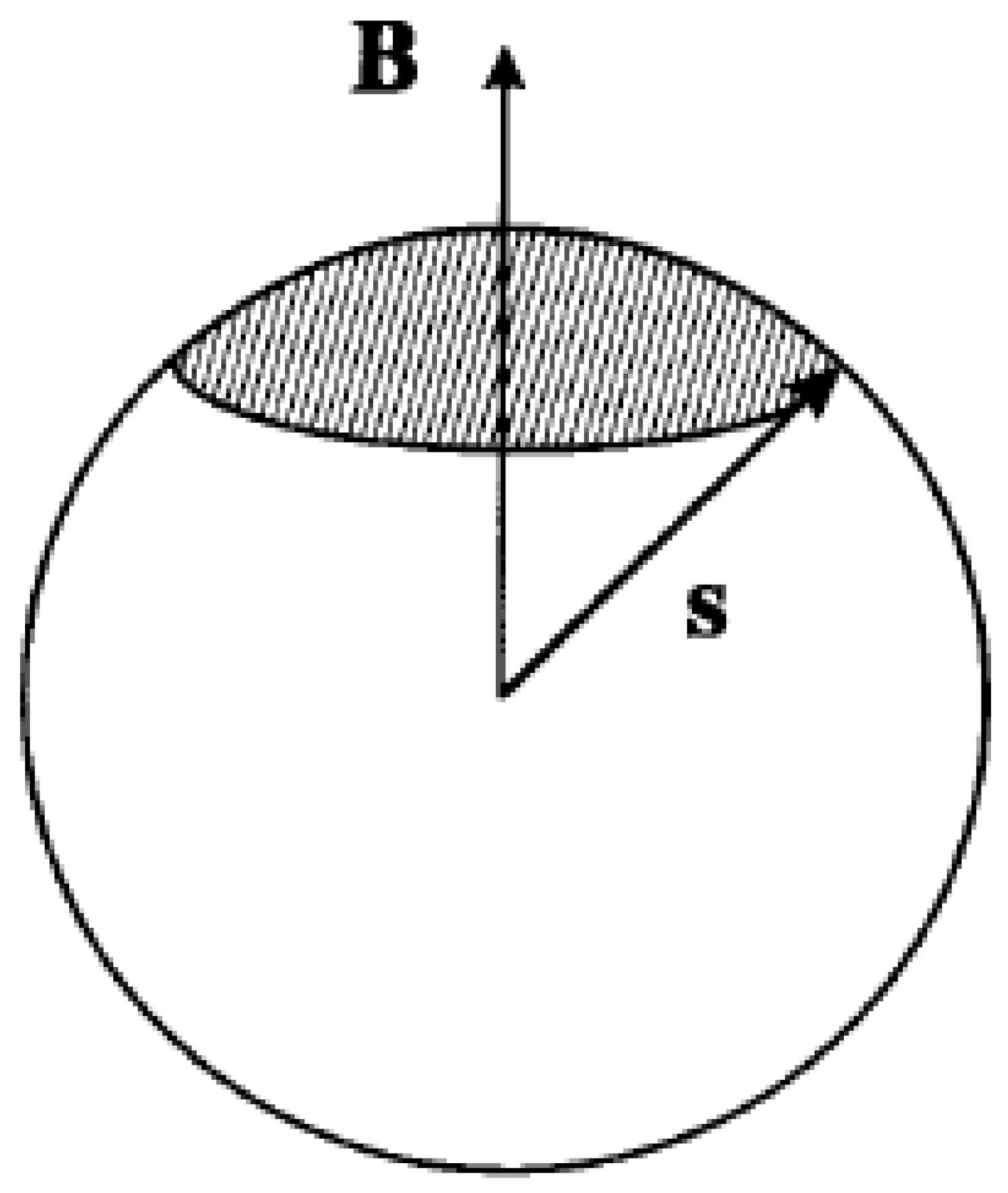
Hence, the total phase shift corresponding to a cyclic evolution is given by,. A simple analysis by Aharaonov and Anandan for a spin half particle at rest in a constant homogeneous magnetic filed leads to the well known result found in Berry’s framework for the geometric phase i.e. with C being a closed curve traced by the spin polarization vector on and being the solid angle subs tended by the closed curve on the Poincare sphere at the origin. Hence, is defined entirely in terms of the geometric structures living on a quantum phase space or the projective Hilbert space .
Figure 3.
Cyclic evolution of the spin polaraisation vector .
2.2.1. Fibre-Bundle approach for the Geometric Phase in Aharonov-Anandan’s Framework
There is an alternative approach by which we can derive the expressions for the Aharonov Anandan phase and it is more convenient for the next discussions related to the Samuel Bhandari generalization and Mukunda Simon’s kinematic approach to the geometric phase.In the context of fibre bundle approach we define the Hilbert Space, State Space and the Ray Space popularly known as framework.The Hilbert Space consists of all the vectors, where as the state space is defined in such a way that it consists a subset of unit vector rays lying in the Hilbert space .We can define a smooth open curve in the state space parametrized by some parameter s, so that at each point of the curve in the state space we can associate a vector which belongs to the State space.The smooth parametrized open curve in the state space is defined as follows,
Now we consider a mapping from the state space to the Ray space so that for every point on the smooth curve in the state space there is the corresponding projection or, density operator in the Ray space and we get an image of the state space curve in the Ray Space and we define the curve as follows:
. Now,the tangent to the state space curve is defined by, but under the gauge transformation does not transforms covariantly i.e.if we consider a local U(1) gauge transformation so that , So, we define the gauge invariant covariant derivative of and that will be the gauge invariant tangent vector to the state space curve.Let us define, and immediately we can see that under the gauge transformation we get,.Now we can define the gauge invariant arc length of the curve C in the ray space as follows,
Figure 4.
The image curve C in the Ray Space and the two different lifts in the state space respectively, and connected by the Gauge transformation.
Figure 4.
The image curve C in the Ray Space and the two different lifts in the state space respectively, and connected by the Gauge transformation.
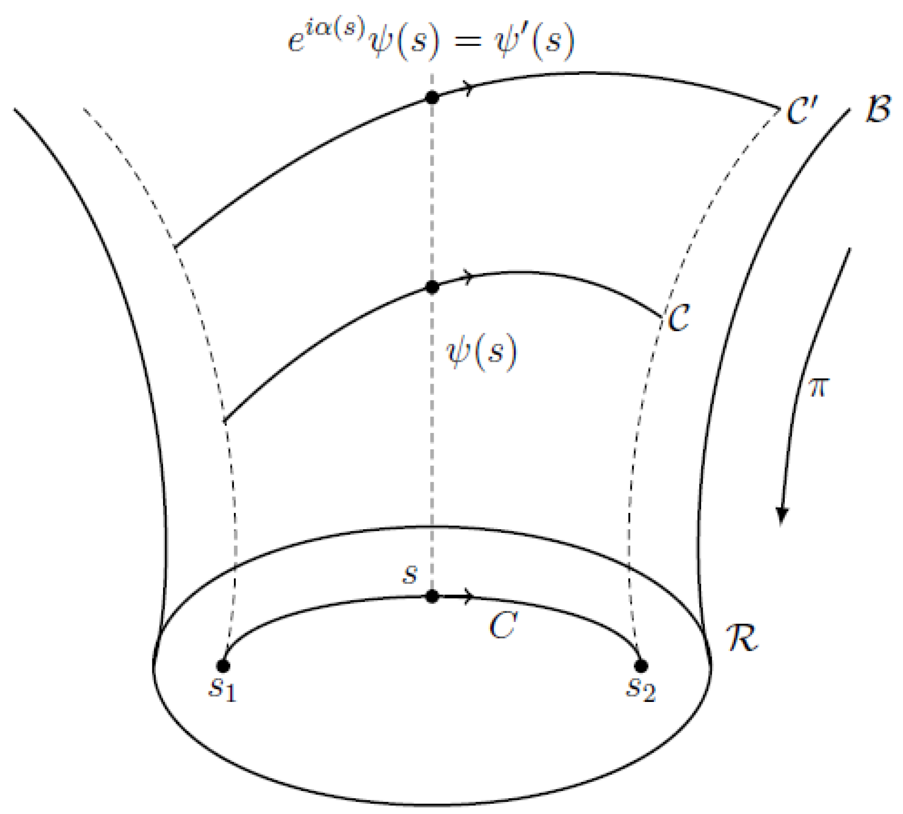
It is evident from the above integral that it is a ray space quantity and the curve C for which the functional is stationery is called the Ray space geodesics.In general we can define different lifts of such curves in the state space or the inverse mapped image of the ray space geodesics in the state space and along the Ray space geodesics the geometric phase vanishes.The curve length is invariant under the gauge transformation and smooth reparametraisation.Finally, the geometric phase can be written as, along with,
Here we can define an Gauge invariant one form such that the dynamical phase factor can be written as an integral of the one form defined in the state space.The one form is given by The framework and the concept of the geodesics in the ray space and the state space is very important as the later will lead to the definition of the Fubini-Study Metric defined in the Ray space and it is defined in terms of the elementary curve length in the state space written as, and the Fubini study metric or the Quantum Geometric Tensor is , some simple examples of the fubini study metric on the Ray space are given below.
- *
- 1. dim;;=Poincare Sphere,geodesics are great circlular arcs of length. Here.
- *
- 2. dim;;. and here is of real dimension 4, has been immensely studied by Simon et.al.
2.3. Samuel Bhandari Generalization
The next generalization is due to Joseph Samuel and Rjendra Bhandari. It is shown that Berry’s phase appears in a more general context than realized so far. The evolution of the quantum system need be neither unitary nor cyclic and may be interrupted by quantum measurements. A key ingredient in this generalization is the use of some ideas introduced by Pancharatnam in his study about the interference of the polarized light, which, when carried over to quantum mechanics, allow a meaningful comparison of the phase between two non-orthogonal vectors in the Hilbert space. Simon first gave a simnple geometrical interpretation of Berry’s phase. If one regards the space of normalized state vectors as a fiber [10,21] bundle over the space of the corresponding Rays where a ray is defined as an equivalence class of states differing only in phase. Then this bundle has a natural connection. This connection permits a comparison of the phases of states on two neighboring rays. Simon observed that when the dynamical phase factor is removed, the evolution of the system as determined by the Schrodinger equation is a parallel transport of the phase of the system according to the natural connection. Berry’s phase is then a consequence of the curvature of this connection. After Aharonov-Anandan generalized the berry phase by relaxing the condition of adiabaticity. The key step was to find the integral of the expectation value of the Hamiltonian as the Dynamical Phase factor and once this dynamical phase factor is removed the phase of the system is again determined by the natural connection and one recovers Berry’s phase for any cyclic evolution of the Quantum System. In the framework of Samuel and Bhandari the central idea was to show the appearance of the berry’s phase in a more general context. The evolution of the system needed be neither unitary (norm preserving) nor cyclic (returning to the original ray).This generalization is based on the work of Pancharatnams work on the interference of polarised light. Carrying Pancharatnam’s ideas over to quantum mechanics yields a fairly general setting for a discussion of Berry’s phase.In summary, Berry’s phase appears to be more general than the context in which it was discovered by Berry, i.e. for an adiabatic,cyclic and unitary evolution. In the context of the fiber bundle approach the expression for the Geometric phase is given by, For a general lift of the Ray space Geodesic
where, be one possible lift of the ray space geodesics with =[ and with ,,,, and the angle between the unit vectors . so, we can say that =arg[] so this is a property of the geodesics in ,derived by them. Using it the geometric phase for the non cyclic evolution of the quantum system can be defined as follows. Let, be any solution of the Schrodinger equation for any stretch of time. Then we adjoin any geodesic (in the generic case) in , the state space in order to take us back from to and combining them we will obtain a closed curve ,say: =(Schrodinger evolution from to ) ∪ (any geodesic from to ) and define, [non cyclic Schrodinger evolution]=. Interestingly the discussion regarding the Samuel and Bhandari’s generalization uses a new ingredient which is the pancharatnams connection.
2.4. The Kinematic Approach and The Bargmann Invariants (Mukunda and Simon)
The third step in the continuing generalization of the Berry Framework after the generalization made by Aharaonov-Anandan and Samuel-Bhandari is due to Raja Simon and Mukunda. The key point was to find construct invariant expressions with respect to two groups of continuous transformations on parametrized curves in Hilbert space local phase changes and reparameterization. The Bargmann invariants (BI) were then brought into the discussion in an important manner, and their connection to GP’s was systematically explored. This latter connection was mentioned by Samuel and Bhandari in a preliminary way. The idea of the framework has already been discussed. The parametrized curves , the action of the local phase changes on them and their images in the ray space have also been introduced before. In addition to the phase changes i.e. a local abelian U(1) gauge transformation i.e. we will introduce the reparameterization invariance. A smooth monotonic reparameterization of is defined as folows:
This then leads to the reparametraisation of the image , giving . Therefore the traces of and C, as set of points in are maintained. The simplest functional of C that remains invariant under the both type of transformation i.e. Gauge and reparametraisation the geometric phase can be defined as follows:
The above equations will hold if we assume the end points of the curve are nonorthogonal i.e.The points to note are : this phase is immediately defined for any open curve as the difference of two terms,any lift of C being used to compute them; the construction is purely kinematic,not using any Hamiltonian or Schrodinger equation. The invariances under phase changes and under reparametrisations lead respectively to being a ray space quantity, and a geometric object. From this definition, the earlier results are all recovered as special cases with the immediate consequence that [any geodesic in ]=0 The content of this is essentially the same but the status is very different.In the work of Samuel and Bhandari,the similar looking formulae was used to set up the definition of the GP for a non-cyclic evolution. Here that is done kinematically in, and the property of geodesics is derived as a consequence.. In the context of the Mukunda Simon’s generalisation the concept of the gauge invariant Bargmann invariant plays a significant role.These were introduced by V. Bargmann in 1964 while giving a new proof of Wigner’s 1931 theorem on representation of symmetry operations in QM. The simplest non-trivial Bargmann Invariant(BI) is of order three. For any three mutually non-orthogonal vectors , it is defined as,
Clearly this is a ray space quantity, and for dim,it is in general complex.Now let to , to and to by the ray space geodesics respectively ; let be any three lifts of the ray space geodesics which connects to , to and to respectively.Then and are closed loops in and respectively.Repeted use of the geodesic property leads to the expression of the geometric phase given by,
Thus the phase of a third order Bargmann Invariant is the negetive of the Geometric phase of the Geodesic Triangle in with the sides being the Ray space Geodesic.Now we are at a position to generalise it for the Bargmann Invariant of order n BI(n) as follows,. So that, [C= n-sided polygon with vertices connected by successive Geodesics]
Now we will review the present work related to the geometric phase of mixed states for the three level open quantum system.The calculation of the geometric phase for the three level sytem of mixed states can be defined by establishing in connecting the density matrix along with the nonunit vector ray in a three dimensional complex hilbert space , here the density matrix for the system being a matrix with the matrix elements being which is hermitain i.e. and conventionally . The density opeartor and the corresponding matrix realisation can be done in the eigenbasis of the hamiltonain.By definition the mixed state density operator is written as follows,
where gives the probability to find the system in the nth energy microstate with energy given by the Gibbs distribution of the cannonical distribution (without any interaction) given by, upon generalising it for the open systems in presence of interaction for a grand cannonical ensemble we have the density operator given by, where, be the grand cannonical partition function. Any hermitian matrix can be written as a linear combination of eight Gell-Mann matrices;the generators of Group and one unit or, Identity matrix.In the case of two level quantum systems the normalized pure states can be mapped to the surface of the 3 dimensional poincare sphere of radius unity, conventionally the Bloch sphere of radius unity is historically known as the poinacare sphere as the hermitian density matrix can be written as a linear combination of 3 pauli matrices (generators of the SU(2) Group) and one Identity matrix and the bloch vector having 3 components;reqires a three dimensional poincare sphere of radius unity and the mixed states lies in the interior of the sphere and in case of the three level system the bloch vector will have eight components along with the pure states lies on the surface of the eight dimensional Bloch Sphere of radius unity and the mixed states of the three level quantum system lies in the interior of the sphere.We can further generalize the scenario for the quantum system with n levels then the density matrix will be a matrix which can be written as a linear combination of number of generators of the Gauge Group and one unit or identity matrix and as a result for the description of the pure quantum states for a n level quantum system we need a Bloch sphere of dimension . The Geometric phase for such a system will depend on variables which we need in order to parametrize the eight dimensional Bloch sphere. The Bloch parameters depends upon the matrix elements of the density operator.The matrix elements can be found by solving the Lindblad Type of Master equation. Once the parameters are determined from the knowledge of the matrix elements of the density operator we will be able to find out the expression for the geometric phase for three level Quantum system. The expression of the Geometric phase is readily obtained by Pnacharatnam formulae. If we begin with the smooth curve (open or closed curve) where, and subdivide the curve into N segments so that the points of subdivision are ,,....., and , with being the density operator corresponding to the pure state are the values at different points.Each trajectory then can be represented by a discrete sequence of quantum states . Thus the geometric phase for the three level quantum system can be expressed in terms of the vectors in , is given by the Pancharatnams formulae.
where we can identify the total phase as and the expression for the geometric phase is gauge and reparametraization invariant. It is interesting to note that, furthermore, under the U(1) gauge transformation defined as , the expression of the geometric phase reduces to,
The above equation is a generalization of the Aharonov and Anandan phase for a pure state with the condition of . Therefore, is called the Aharonov-Anandan Phase for the mixed states.Now if we consider the interaction between the system and the environment, the system will no longer undergo a cyclic evolution, the matrix elements will be a decaying function of time and also the bloch vectors and the nonunit state vectors. But when the system is isolated from the environment, however, the system may be regarded as a quasicyclic process so that the total phase becomes , which is not important and the total phase can be dropped in the expression of geometric phaase given in equation(13) so that the geometric phase under the quasicyclic process can be expressed as follows; alongwith , here the set of eight parameters are required for the parametraisation of the Bloch sphere out of which one is the radius of the bloch sphere i.e.r and the other seven are the angular coordinates.
The above formulae can be used to calculate the geometric state for mixed state for a quasicyclic evolution this is called the Berry phase for the mixed state, while is a closed circle arc on the the generalized eight dimensional Bloch sphere for the three level system where the parametraisation variables depends on the matrix elements of the density matrix i.e. .It is noted that the Berry phase for the mixed state is an integral of something called the Mead-Berry connection one form around the closed curve C in .
3. Insights of Lindblad’s Master Equation in the Context of Open Quantum Systems
The Lindblad equation is the most general form for a Markovian master equation [7,10], and it is very important for the treatment of irreversible and non-unitary processes, from dissipation and decoherence to the quantum measurement process. For the latter, in recent applications, the Lindblad equation was used in the introduction of time in the interaction between the measured system and the measurement apparatus. Then, the measurement process is no longer treated as instantaneous, but finite, with the duration of that interaction changing the probabilities - diagonal elements of the density operator - associated to the possible final results. On the other hand, in quantum optics, the analysis of spontaneous emission on a two-level system[8]leads to the Lindblad equation. At last, in the case of quantum Brownian movement, it is possible to transform the Caldeira-Leggett[3]quation into Lindblad with the addition of a term that becomes small in the high-temperature limit. These are a couple of many applications of the Lindblad equation, justifying its understanding by students in the early levels. Contrasting against its importance and wide range of applications, its original deduction involves the formalism of quantum dynamical semigroups, which is quite unfamiliar to most of the students and researchers.
As mentioned earlier in order to find out the geometric phase we require the time dependent bloch sphere parameters which depends on the matrix elements of the density operator which are time dependent, when interaction comes into the picture in case of the open system between the system and the surroundings the time evolution of the density operator is governed by the Lindblad type of Mater Equation[17]. As an example, let us consider a three-level system interacting with environment. When a relevant dynamical time scale of the open quantum system is long compared to the time for the environment to forget quantum information, the evolution of system is effectively local in time (the Markovian approximation) and may be described by the Lindblad’s master equation [16] given by,
The first term of the master equation is a usual schrdinger term which generates an unitary evolution which appear in the well known Von-Neumann Liouville equation of quantum statistical mechanics and the remaining part of the equation describe all possible transitions that the open system may undergo due to the interaction with the reservior.The operators (i=1,2,3,...,8) are called the Lindblad Operators or the quantum jump operators. It can be readily checked that is hermitian and , which implies that that he Lindblad Master equation preserves the positivity of the density operator for the open system. In the present work the Lindblad operators are choosen as which represents the coupling to the environement.Where the matrices are called the Gell-Mann Matrices given by,
The noise can be controlled by switching on and off .Now suppose the dephasing noise is represented by a single type of Lindblad operator given as is applied to our three level system with hamiltonian being = then upon solving the master equation along with the given initial condition we will get the matrix elements.
Required to note that,If we consider only the first term on the right hand side of Lindblad Master equation we obtain the Liouville-von Neumann equation. This term is the Liouvillian and describes the unitary evolution of the density operator. The second term on the right hand side of the equation is the Lindbladian and it emerges when we take the partial trace - a non-unitary operation - of the degrees of freedom of reservior.The Lindbladian describes the non-unitary evolution of the density operator. By the interaction form adopted here the physical meaning of the Lindblad operators can be understood: they represent the system S contribution to the System-Bath interaction remembering once more that the Lindblad equation was derived from the Liouville-von Neumann one by tracing the bath degrees of freedom. If the Lindblad operators are Hermitian (observables), the Lindblad equation can be used to treat the measurement process. A simple application for a two level quantum system in this sense is the system Hamiltonian where be the z component of the pauli matrices, when we want to measure one specific component of the spin ( without any summation).If the Lindblad operators are non-hermitain then the master equation can be used to treat dissipation [2], decay and decoherence[6]. For this type of scenario let us choose the system Hamiltonian same as in the previous case i.e. where be the z component of the Pauli matrices with the Lindblad operators are taken as , where be the spontaneous emission rate [20].
4. Kinematic Approach to the Mixed State Geometric Phase in Nonunitary Evolution
In 2004,A kinematic approach to the geometric phase for mixed quantum states [25] in nonunitary evolution is proposed.This phase is manifestly gauge invariant and can be experimentally tested in interferometry. It leads to well-known results when the evolution is unitary. The kinematic approach for the mixed quantum states in the case of the nonunitary evolution deals with the upliftment of the mixed states to a pure states using the approach of purification the approach is sometimes very useful when we deal with the decoherence in quantum computation,Geometric phases are useful in the context of quantum computing as a tool to achieve fault tolerance. However, practical implementations of quantum computing are always done in the presence of decoherence.Thus,a proper generalization of the geometric phase for unitary evolution to that for nonunitary evolution is central in the evaluation of the robustness of geometric quantum computation.Here,the proposition of the quantum kinematic approach to the geometric phase for mixed states in nonunitary evolution along with the scheme to realize nonunitary paths in the space of density operators in the sense of purification, which could be of use in experimental tests of the mixed state geometric phase. Let us consider a quantum system s and the underlying Hilbert space being N dimensional.An evolution of the state of the system may be described by the path,
in the above equation and are the eigenvalues and the eigenvectors of the density operaor.All the nonzero are assumed to be nondegenerate function of . Now to introduce the notion of the ,mixed state geometric phase we begin with the purification of the mixed state to a pure state of a larger system also called the supersystem and we will choose the ancillary bath as the reservior in order to take into account the interaction of the system with the surrounding. we start with a combined system which consist of the original system s and the ancillary bath a with dimensional Hilbert Space if without loss of generality we assume that then the Schmidt purification theorem can be used to lift up the mixed state to a pure state where,
where be the states of the ancillary bath and is a purification of the density operator of the system s in the sense that the original density operator of the system will be obtained upon calculating the partial trace of the pure state density operator with respect to the ancillary bath states.The pancharatnam relative phase between and is given by,
since, both and are the orthonormal bases in the hilbert space there exist, for each an unitary operator such that, along with and , can be taken as,. Then, the pancharatnam relative phase can be recasted as,
In order to arrive at the expression of the geometric phase associated with the path the removal of dependence upon purification of the type depicted in the equation. But the thing to notice is that is the standard geometric phase of the pure entangled state for when the evolution satisfies the parallel transport condition i.e..However, this single condition is insufficient for mixed states as it specifies only one of the N undetermined phases of ,and the resulting pure state geometric phase remains strongly dependent upon the purification. Instead, the essential point to arrive at the geometric phase associated with is to realize that there is an equivalence set of unitarities that for all realize , namely those of the form,
where, fulfills , but is otherwise arbitrary. are real time dependent parameters such that . We may particularly identify , to satisfy the parallel transport conditions given by,
in terms of which the relative phase in equation(22) coincides with the geometric phase associated with the path . Simple calculation leads to the expression of given by,
putting the expression of for in Equation (22) we get the expression of geometric phase for the mixed states as follows,
The above equation gives the explicit form of the geometric phase for the path .
Now, a reasonable notion of mixed state geometric phase in the nonunitary case should satisfy the following conditions: (a) it must be gauge invariant, i.e.,be dependent only upon the path traced out by the system’s density operator ; (b) it should reduce to well-known results in the limit of unitary evolution; (c) it should be experimentally testable.
firstly,First, the phase is manifestly gauge invariant in that it takes the same value for all .One may check this point by directly that . Now in particular if we let we immediately get,
which verifies that the relative phase gives the geometric phase for Thus, the geometric phase defined by Eq.(26) depends only upon the path traced out by .
Second, when the evolution is unitary, corresponding to the case where the eigenvalues !k are time independent and is identified with the time evolution operator of the state, the geometric phase defined by Eq.(26) leads to well-known results [24,25].
In the above context we have dealt with the nondegenerate case but it can be generalised for the degenerate case as well which is briefly delineated below. In the case of degeneracy the density opeartor of the system can be described as folows,
where , are the degenerate eigenvectors corresponding to the eigenvalues of the density opearator i.e. at the kth level along with a fold of degeneracy . The modified expression of the geometric phase for the degenerate case of the path will be defined as,
where, is defined by with the unknown coefficients are determined by the parallel transport condition obeyed by given below,
with , which leads to,
Where P denotes the path ordering operator similar to the time ordering operator. The above equation can be generalised to the situation where the non-negative eigenvalues of the density operator are non-degenerate only in the interval by denoting the eigenvectors in the corresponding subspace are, due to continuity,uniquely given at the end points and .
In summary, the proposal of a kinematic approach to the mixed state geometric phase in nonunitary evolution. The proposed geometric phase is gauge invariant in that it depends only upon the path in state space of the considered system and also demonstrated that the proposed geometric phase for non-unitarily evolving mixed states is experimentally testable in interferometry. Moreover, it leads to the well-known results when the evolution is unitary. As an example, we have used the present approach to calculate the geometric phase for non-unitarily evolving mixed states in the case of a qubit undergoing free precession around a fixed axis and affected by dephasing.
Appendix A
For, the convenience of the reader we will give some insights related to the purification of the quantum states i.e. Schmidt’s Purification theorem.
Appendix A.1. The Schmidt’s Purification
There are many ways to deal with the mixed states in the context of determining the geometric phase of mixed states for a certain quantum system. And one such idea of the calculation of the geometric phase for the mixed states for a certain quantum system is to lift up the mixed states to a pure state and then doing the calculation of the geometric phase for that pure states which is already known to us. In order to lift up the mixed states of the quantum system to the pure state belonging to a higher dimensional Hilbert space generally the tensor product hilbert space or, simply a composite hilbert space constituted by the system and the ancillary bath allowing interaction between them. But the starting point towards the process of purification is due to the Schmidt Decomposition Theorem discussed below.
The Schmidt Decomposition Theorem:
Let us consider two sets of orthonormal basis vectors and belonging to two different hilbert spaces and respectively i.e. and . The two sets of orthonormal Basis vectors and are spanned over the hilbert spaces denoted by and respectively. Now, let be an arbitrary ket such that which is the composite Hilbert space of higher dimensionality. Required to mention that the dimensionality of the two different Hilbert spaces respectively, and may or, may not be the same. Let, us consider the general situation here i.e. dim().Then according to the Schmidt’s purification theorem if there exist a set of positive values then,
where, r is known as the "Schmidt Number" (or, "rank") of and are called the "Schmidt coefficients". Let us point out some of the interesting properties of the Schmidt’s Decomposition which is basically a singular value Decomposition mentioned below:
- We can take any bases of and and we can write,
- We can use the singular value decomposition: where,
- Formation of the orthonormal Basis and using and V as change of Basis.
The we obtained using the Schmidt’s Decomposition theorem will be a pure state using this in our case we have obtained the following equation discussed in the context [13].
Where, the two sets of orthonormal basis has been chosen to describe the system and the ancillary bath and the two different associated hilbert spaces with the system and the ancillary bath and for simplicity we have taken the dimensionality of the associated Hilbert spaces to be equal.
References
- Aharonov, Y.; Anandan, J. Phase change during a cyclic quantum evolution. Physical Review Letters 1987, 58, 1593. [Google Scholar] [CrossRef] [PubMed]
- Alexandre Brasil, C.; Fernandes Fanchini, F.; Napolitano, R.d.J. A simple derivation of the Lindblad equation. arXiv e-prints 2011, pp. arXiv–1110.
- Benderskii, V.; Kotkin, A.; Kats, E. Revivals in Caldeira–Leggett Hamiltonian dynamics. Physics Letters A 2013, 377, 737–740. [Google Scholar] [CrossRef]
- Berry, M.V. Quantal phase factors accompanying adiabatic changes. Proceedings of the Royal Society of London. A. Mathematical and Physical Sciences 1984, 392, 45–57. [Google Scholar]
- Born, M.; Wolf, E. Principles of optics: electromagnetic theory of propagation, interference and diffraction of light; Elsevier, 2013.
- Brasil, C.A.; Fanchini, F.F.; Napolitano, R.d.J. A simple derivation of the Lindblad equation. Revista Brasileira de Ensino de Física 2013, 35, 01–09. [Google Scholar] [CrossRef]
- Breuer, H.; Petruccione, F. The Theory of Open Quantum Systems; Oxford University Press, 2002.
- Carmichael, H. Statistical Methods in Quantum Optics 1: Master Equations and Fokker-Planck Equations; Physics and astronomy online library, Springer, 1998.
- Fowles, G.R. Introduction to modern optics; Courier Corporation, 1989.
- Gardiner, C.W.; Zoller, P. Quantum noise, Vol. 56 of Springer series in synergetics. Springer–Verlag, Berlin 2000, 97, 98. [Google Scholar]
- Howell, J.C.; Lamas-Linares, A.; Bouwmeester, D. Experimental violation of a spin-1 Bell inequality using maximally entangled four-photon states. Physical Review Letters 2002, 88, 030401. [Google Scholar] [CrossRef] [PubMed]
- Hulst, H.C.; van de Hulst, H.C. Light scattering by small particles; Courier Corporation, 1981.
- Jiang, Y.; Ji, Y.; Xu, H.; Hu, L.y.; Wang, Z.; Chen, Z.; Guo, L. Geometric phase of mixed states for three-level open systems. Physical Review A 2010, 82, 062108. [Google Scholar] [CrossRef]
- Karlsson, M. Polarization mode dispersion–induced pulse broadening in optical fibers. Optics letters 1998, 23, 688–690. [Google Scholar] [CrossRef] [PubMed]
- Layton, E.; Huang, Y.; Chu, S.I. Cyclic quantum evolution and Aharonov-Anandan geometric phases in SU(2) spin-coherent states. Phys. Rev. A 1990, 41, 42–48. [Google Scholar] [CrossRef] [PubMed]
- Lindblad, G. On the generators of quantum dynamical semigroups. Communications in Mathematical Physics 1976, 48, 119–130. [Google Scholar] [CrossRef]
- Manzano, D. A short introduction to the Lindblad master equation. AIP Advances 2020, 10, 025106. [Google Scholar] [CrossRef]
- Milburn, G.J.; Laflamme, R.; Sanders, B.; Knill, E. Quantum dynamics of two coupled qubits. Physical Review A 2002, 65, 032316. [Google Scholar] [CrossRef]
- Mukunda, N.; Simon, R. Quantum kinematic approach to the geometric phase. I. General formalism. Annals of Physics 1993, 228, 205–268. [Google Scholar] [CrossRef]
- Nielsen, M.A.; Chuang, I.L. Computação quântica e informação quântica; Bookman, 2003.
- Niu, C.; Xu, G.; Liu, L.; Kang, L.; Tong, D.; Kwek, L. Separable states and geometric phases of an interacting two-spin system. Physical Review A 2010, 81, 012116. [Google Scholar] [CrossRef]
- Pratapsi, S.S.; Gouveia, J.a.; Novo, L.; Galvão, E.F. Elementary characterization of Bargmann invariants. Phys. Rev. A 2025, 112, 042421. [Google Scholar] [CrossRef]
- Samuel, J.; Bhandari, R. General setting for Berry’s phase. Physical Review Letters 1988, 60, 2339. [Google Scholar] [CrossRef] [PubMed]
- Schrödinger, E. An Undulatory Theory of the Mechanics of Atoms and Molecules. Phys. Rev. 1926, 28, 1049–1070. [Google Scholar] [CrossRef]
- Tong, D.; Sjöqvist, E.; Kwek, L.C.; Oh, C.H. Kinematic approach to the mixed state geometric phase in nonunitary evolution. Physical review letters 2004, 93, 080405. [Google Scholar] [CrossRef] [PubMed]
Disclaimer/Publisher’s Note: The statements, opinions and data contained in all publications are solely those of the individual author(s) and contributor(s) and not of MDPI and/or the editor(s). MDPI and/or the editor(s) disclaim responsibility for any injury to people or property resulting from any ideas, methods, instructions or products referred to in the content. |
© 2025 by the authors. Licensee MDPI, Basel, Switzerland. This article is an open access article distributed under the terms and conditions of the Creative Commons Attribution (CC BY) license (http://creativecommons.org/licenses/by/4.0/).
Copyright: This open access article is published under a Creative Commons CC BY 4.0 license, which permit the free download, distribution, and reuse, provided that the author and preprint are cited in any reuse.


