
Submitted:
08 July 2025
Posted:
11 July 2025
You are already at the latest version
Abstract
This paper investigates the properties of the Gorini–Kossakowski–Sudarshan–Lindblad (GKSL) equation within the camel-like framework, with a focus on quantum correlations in the context of open quantum systems. Here, we compute quantum correlations such as quantum discord and quantum steering, analyzing their behavior under decoherence and environmental interaction for three sets of quantum states. Our results indicate that the sign of the entanglement entropy's derivative serves as an indicator of the system's drift toward classical or quantum information exchange—an insight with important implications for quantum error correction and dissipation processes in quantum thermal machines. \\ Moreover, we parametrize quantum states using both single-parameter and Bloch-sphere representations. The Bloch-sphere analysis is particularly developed by examining the topology of the quantum states as elements on the \(\mathbb{S}^2\) sphere, yielding a gradient map and a topological basin map which illustrate how quantum states evolve under the camel-like framework and how this can be partitioned into basins on the Bloch sphere, by stability/instability against decoherence. The decoherence-unstable regions form a Braiding ring around the Bloch sphere at the circle defined by $\theta=\frac{3\pi}{4}$. Notably, these unstable states on the Braiding ring form attraction points for the evolution of states by a constructed Lyapunov function, which gives an illustration of the complex interplay between geometry and dynamics and which shapes the topological geometry on the Bloch sphere. This deeper analysis underscores that quantum dynamics are governed not only by local energetics but also by the global structure of the state space. Moreover, we also derive a testable rudimentary experimental setup from the camel-like entropy, which describes the unitary evolution of pure states on the Bloch surface and add the analytical solutions of selected quantum states.
Keywords:
Gorini–Kossakowski–Sudarshan–Lindblad (GKSL) equation
; open quantum systems
; camel-like entropy
; quantum correlations
; Bloch sphere
; quantum dynamics
; quantum state topology
1. Introduction
In order to analyze the interactions between two or more elements in a quantum information system, one can represent these elements or events as states of information, termed infons. These infons might describe, for example, the interaction between two bosons [1], the exchange of cognitive signals between neurons in the brain [2], or the quantum tunneling of electron pairs across a potential barrier [3]. The dynamics of these interacting elements can be effectively modeled within the framework of open quantum systems [1,4]. This formalism provides a fully quantum-mechanical description of a system as it evolves under the influence of a local environment [5,6,7]. The environment accounts for effects such as decoherence and dephasing, which impact the state of the system .
The system-environment relationship can be represented hierarchically as:
where represents the highest containing state (e.g., an isolated entangled system subjected to an electromagnetic field).
The evolution of the system under the influence of can be described using the density matrix formalism. Let denote the initial state of . Under the action of a Hamiltonian (representing a local perturbation within ), the system evolves to a final state :
The environment can be an electromagnetic field for particles [8,9,10,11] or even a cognitive environment for neuronal cells, including electric currents, neurotransmitters, and other stimuli [7,12,13].
1.1. Quantum-like Formalism for the GKSL Equation
The foundational framework of open quantum systems can be extended beyond traditional physical scenarios to model quantum-like processes in biological and cognitive systems. Such models have been increasingly applied to represent quantum phenomena across natural sciences [7,14,15].
For instance, neuronal signals (treated as infons) can be described by quantum observables and probabilities, where information processing is governed by specific dynamics between decoherence and non-unitary evolution of quantum states. The transition of a neuronal state under environmental perturbations can be represented as a superposition of wavefunctions [7], where the wavefunction of the neuron exposed to some perturbation undergoes the following transition:
where denotes the wavefunction at steady state with the environment, the excited state, and the quiescent state. Here, and are complex coefficients satisfying the normalization condition . is a locally acting perturbation within , and represents the totality of electrochemical signals in the environment of the neuron, including electric currents, EMF, and neurotransmitters generated by other neurons [12].
In line with quantum theory, the transition induced by in (3) can be represented within the density matrix formalism:
where transitions to , describing the probabilistic nature of superposition. Now, in order to construct the density matrix from a state vector we define as a complex Hilbert space, where a pure quantum state is represented by a unit vector , and its dual vector by:
Then, the fhe final density matrix corresponds to the pure state described by the outer product:
with the pure state given by:
and
where and are complex coefficients, and and are their complex conjugates, respectively.
By examining equation (3), we can see that and are represented by in (6), with arbitrary coefficients in both real and complex form. Thus, we have demonstrated how the biological state transition in (3) can be represented by a superposition of quantum states in an open quantum system via (6). This formulation automatically satisfies the Born rule, which gives the probability of measuring the system:
1.2. GKSL Operator Structure and Dynamics
Let us first introduce the space of states, which we devise using the finite-dimensional Hilbert space endowed with the scalar product . Let the space of density operators (which represent the states of the system) be denoted by , and the space of all linear operators be given by . Furthermore, is a complex Hilbert space with the scalar product , with A and B being operators. We have furthermore that the environment (i.e. dephasing/decoherence) is represented by superoperators in that act on the density matrix . The GKSL equation is the time-dependent master equation for open quantum systems, developed in [17,19] from the Schrödinger equation. It is described by
Here, is the unknown probability density matrix, which evolves with time and is used to resolve properties of an open quantum system, such as entropy, entanglement, and decoherence [17,19]. The first term on the RHS in (11), the Hamiltonian, is the unitary and deterministic part of the evolution, while the second term on the RHS in (11), the dissipation operator, represents the non-unitary effects on the density matrix that ultimately represent non-deterministic evolution of the system. The Hamiltonian represents the internal dynamics of the system at hand, and are often given by the Pauli matrices, however in some cases it can also include component related to the interaction with the environment [20]. The dissipation operator, , is the GKSL superoperator given by:
where is the adjoint of the jump operator L, defined by the relation:
This relation holds for any linear operator L, Hermitian or not, and defines with respect to the inner product. In general, the jump operators L in the Lindblad formalism are non-Hermitian, representing dissipative processes such as decoherence or decay. We have hence the GKSL equation given by
where is the relaxation factor for decoherence processes to the dissipation operator. Each jump operator represents the special type of interaction of the system by the density matrix in (10), with the environment (described by , and vary according to the decoherence and dissipation resulting by the formalism of H and . This forms the main difference between the original Schrödingers equation and the GKSL equation: the GKSL equation produces stabilization of its solution to the steady-state (10).
1.3. Camel-Like Framework in Entropy Evolution of Open Quantum Systems
In the study of complex systems, entropy serves as a fundamental measure of disorder and information content. We introduce the concepts of N-hump camel-like entropy to describe distinct temporal profiles of entropy evolution in light of the studies by Khrennikov [7,12,13,15,21]. A 1-hump camel-like entropy is characterized by a single local maximum and minimum, followed by damped oscillations, while a 2-hump camel-like entropy exhibits two such maxima and minima before stabilizing. These definitions are inspired by the analogy of a camel’s humps, providing an intuitive visualization of entropy dynamics. In quantum information research, these profiles could prove invaluable for analyzing the behavior of quantum systems undergoing decoherence, entanglement dynamics, or information scrambling. For instance, a 2-hump entropy profile might indicate the presence of intermediate metastable states in a quantum process, while a 1-hump profile could describe simpler, single-phase transitions. Furthermore, we can also obtain N-humps and obtain Rabi-like oscillations [22] in the entropy evolution which have similarities to the study of spin-state fractions in single atom system [23]. By categorizing entropy evolution in this way, we may gain a deeper understanding of the underlying mechanisms governing quantum systems, paving the way for improved control and optimization in quantum computing and communication protocols using the hereafter defined camel-like framework presented by Khrennikov [2,7,12,13,15,21].
Definition 1.
(Camel-like behaviour of entropy)
One-Hump Camel-Like behaviour of the Entropy
Consider the following time intervals:
We characterize these intervals using the derivative of entropy as follows:
- on , and
- on , and
- On , exhibits damped oscillations in amplitude.
This behavior corresponds to a one-hump camel analogy, where the entropy profile has a single local maximum at and a single local minimum at .
Two-Hump Camel-Like behaviour of the Entropy
Consider the following time intervals:
We characterize these intervals using the derivative of entropy as follows:
- on , and
- on , and
- on , and
- on , and
- On , exhibits damped oscillations in amplitude.
This behavior corresponds to a two-hump camel analogy, where the entropy profile has two local maxima at and , and two local minima at and .
N-hump camel-like behaviour of the Entropy
Let be the entropy of a quantum system evolving under the GKSL equation. We define as having Nhumps (local maxima) if there exists a sequence of critical points such that the time domain is partitioned into intervals:
where , and the entropy derivative satisfies:
- Growth Phases: on for all k, with (local maxima).
- Decay Phases: on for all k, with (local minima).
- Asymptotic Damping: On , exhibits underdamped oscillations converging to a steady-state value .
From this definition, we see that the defined camel-like entropy profiles, characterized by transient maxima and minima in disorder, evoke parallels to barrier-crossing phenomena across diverse systems, based on their number of humps. For instance, in enzyme catalysis [24], the one-hump entropy profile mirrors the transient disordered transition state (hump) that precedes product stabilization—akin to overcoming a single entropic barrier during catalysis. In contrast, two-hump entropy aligns with multi-phase processes like protein folding [25], where disordered intermediates and misfolded states generate sequential entropy peaks, or quantum tunneling [26] with successive decoherence events. Moreover, spin-fraction measurement for single atom systems [23] show Rabi-oscillations, which are in a damped form here described as N-hump camel like behaviour.
1.4. Operators
Now that we have formalized the definition of the camel-like entropy, we can define the Hamiltonian H and the dissipation operator that governs the dynamics of the system following the camel-like formalism proposed by Khrennikov [2,7,12,13,15,21]. By he GKSL equation:
we have, which is the relaxation rate representing the strength of interaction between a quantum system and its environment. We present the model example of the order-stable dynamics that matches the biological order-preserving behavior and select the Hamiltonian H and the interaction operator C as follows [2]:
We calculate these operators into their four-dimensional form:
The dissipation operator redimensioned to gives the collapse operator C, which we extend to act on the two-qubit system. By choosing an operator that acts locally on one qubit, specifically , where is the raising operator for the first qubit and I is the identity matrix for the second qubit, we obtain:
Based on analysis done in [27] we set the relaxation factor .
Having set the premises for the study of the camel-like framework of the GKSL equation applied on a set of quantum states, we now define our aims. The first aim is to study the evolution of the the von Neumann entropy for the set of selected quantum states, and the quantum correlations of quantum discord, entanglement entropy, mutual information and the Bell-CHSH parameter, so that we show the performance of the camel-like framework on pure states, product states and mixed states. Second, we wish to analyse the properties of the camel-like framework by using a gradient field and topological basin analysis, so that we can study the evolution of solutions on the Bloch sphere and their stability. At last, we provide analytical solutions which satisfy the definition of the 1. Using this combination of analytical tools, we thus aim to present how the camel-like framework works and to which physical experiment it has strong similarities to.
2. Methods of Analysis
2.1. State Representation
We can form the given (normalized) states for the three classes of quantum states, pure states, product states and mixed states: The states of interest are represented thus by the three categories:
Bell-states.
We include two Bell states in our calculations, namely and .
Product states.
In tensor product form:
in tensor product form:
Mixed states.
The mixed states are defined with probabilities using the pure states:
where:
2.2. Numerical Calculations
We employ numerical methods to solve the Lindblad equation, specifically utilizing matrix exponential techniques where we use the forward-Euler method [28] for solving the Lindblad equation to calculate purity, entropy, quantum discord and mutual information. The calculation of von Neumann entropy uses logarithm base 2 to align with information theory, where entropy measures uncertainty in bits. When we calculate the entanglement entropy, we use the mesolve method as part of the qutip package [29]. Finally, for the calculations of the CHSH parameter,, we use the Runge-Kurra method of 4th order. These approaches allows us to study the evolution of the density matrix through the matrix exponential. We analyze the numerical solutions for the density matrices over time to observe the evolution of the mentioned quantum relations as a result of the Lindblad dynamics. All simulations are carried out with Python.
2.3. Quantum Correlations Computational Code
We form Python codes for the study of the time evolution of the von Neumann entropy for the considered pair of states (Bell states, product states and mixed states). All states are represented as density matrices, computed as the outer products of the states with their conjugates. The Hamiltonian governing the system is defined as , where is the Pauli-X matrix. The collapse operator is defined as , with being the raising operator for a single qubit and I the identity matrix. The evolution of the system is modeled using the Lindblad equation, which accounts for both the Hamiltonian and dissipative processes. The Lindblad evolution step is implemented by iterating over small time steps , updating the density matrix at each step, and normalizing the result to ensure it remains a valid density matrix. The von Neumann entropy is computed at each time step using the eigenvalues of the density matrix. To avoid numerical issues, eigenvalues are clipped to a small value before taking their logarithm. The time evolution is simulated for 1000 steps, with a time step of .
2.3.1. von Neumann and Entanglement Entropy
The entanglement entropy is computed using the von Neumann entropy, which quantifies the amount of quantum entanglement in a system. In the code, we compute this as:
where the logarithm is taken in base 2, and the trace operation sums over the eigenvalues of the matrix. To calculate the entanglement entropy for the two-qubit systems, the following procedure is applied in the Python code:
1. Partial Trace: The first step is to compute the partial trace over one of the qubits (in this case, the second qubit) to obtain the reduced density matrix for the first qubit. The partial trace operation effectively “traces out” the second qubit, leaving a reduced matrix that describes the subsystem of interest. For a two-qubit system described by the density matrix , the partial trace over the second qubit is computed as:
For the two-qubit Bell states, this results in a 2x2 matrix representing the reduced density matrix of the first qubit.
2. Eigenvalue Calculation: After obtaining the reduced density matrix, its eigenvalues are computed. These eigenvalues represent the probabilities associated with the possible states of the reduced system.
3. Von Neumann Entropy: Once the eigenvalues of the reduced density matrix are obtained, the von Neumann entropy is computed by applying the formula:
where are the eigenvalues of the reduced density matrix . To prevent numerical issues, the eigenvalues are clipped to a small value before taking the logarithm (e.g., ) to avoid computing . This process is repeated for each time step during the evolution, allowing us to track how the entanglement entropy changes over time due to the effects of the dissipative dynamics introduced by the Lindblad evolution.
2.3.2. Mutual Information
The mutual information is computed in the Python script as:
where , , and are the von Neumann entropies of the reduced density matrices , , and the total density matrix , respectively. The mutual information is calculated at each time step for both states by tracing out subsystems and computing the von Neumann entropies. The results are stored and plotted as a function of time. This process tracks how the mutual information between the subsystems evolves over time, showing the dynamics of quantum correlations in the Bell states.
2.3.3. Derivative of the Entanglement Entropy
The first derivative of the entanglement entropy with respect to time is computed numerically using the ‘np.gradient’ function on the entanglement entropy values, which are computed as in the entropy-code.
2.3.4. Quantum Discord
Quantum discord is computed as the difference between mutual information and classical correlation. The quantum discord is computed at each time step for both states. The function function calculates this using the defined mutual information and classical correlation functions. The quantum discord at is computed and printed for both states, providing insight into the initial correlations. The eigenvalues of the initial density matrices are computed to analyze the purity and state properties of the system at the start.
2.3.5. CHSH Parameter
In the Python code used to calculate the time evolution of the Clauser-Horne-Shimony-Holt (CHSH) parameter for both states, we calculate it by evaluating the expectation values of four measurement settings, , , , and , for the two qubit system at each timestep. The code then computes the CHSH parameter over time and plots its evolution, comparing it to the classical bound of 2 and the quantum maximum of . This allows for the analysis of quantum correlations and the violation of local realism as a function of time for both states. All calculations are carried out using the following Python packages:
- numpy: A fundamental package for numerical computing in Python, used for array manipulation and linear algebra operations such as matrix products and Kronecker products.
- scipy.linalg: Specifically, the expm function from this module is used for matrix exponentiation.
- matplotlib.pyplot: A plotting library used for generating visualizations, such as graphs for quantum discord and CHSH parameters.
-
qutip: A quantum toolbox used for simulating quantum systems. Key functions from qutip include:
- −
- sigmax(), sigmay(), sigmaz(): Pauli matrices for qubits.
- −
- qeye(): Identity matrix for qubits.
- −
- basis(): Creates the computational basis states.
- −
- tensor(): Computes tensor products of quantum states and operators.
- −
- mesolve(): Solves the Schrödinger equation with dissipation (Lindblad evolution).
- −
- entropy_vn(): Computes the von Neumann entropy.
2.4. Analytical Solutions
The analytical solutions to the GKSL equation under the camel-like framework were found using a Python script that uses SymPy to model and solve the time evolution of a two-level quantum system described by a density matrix. The time variable t is defined as a real-valued symbol, and the matrix components , , and are declared as time-dependent functions. These represent, respectively, the population of the first state and the coherences of the system. The system of differential equations encodes the dynamics of the density matrix, possibly derived from a Lindblad-type master equation or an effective non-Hermitian Hamiltonian. Specifically, evolves according to a population exchange term and a term involving the imaginary part of the coherences, while and evolve under damping and driving terms that couple to the population difference. Initial conditions are provided in the form of a dictionary, specifying the values of the components of at time ; for example, setting , , and corresponds to the system being initially in the excited state, that is, . The script then attempts to solve the system symbolically using dsolve, and generates the solution in the command prompt. The program also checks the hermiticity of the resulting matrix by verifying whether , whether remains real-valued, and whether the trace is preserved. Finally, the steady-state limit is computed and formatted in the command prompt.
2.5. Gradient Map Analysis on the Manifold Represented by the Bloch Sphere
The gradient flow analysis was implemented in MATLAB through a custom script that visualizes critical dynamics on the Bloch sphere representation of quantum states. The script defines the mathematical components and from (70), along with the squared magnitude function whose gradient drives the flow analysis. Using numerical differentiation with a delta of , the gradient is computed and incorporated into a differential equation system modeling the negative gradient flow, solved via MATLAB’s ode45 Runge-Kutta solver with high precision tolerances (). The Bloch sphere is rendered as a surface mesh colored by the z-coordinate, with the southern quarter-circle at explicitly highlighted in red as the critical manifold. Six unstable initial states are marked with distinct colors and enlarged markers, representing the singularities in (53) where the map is undefined (two of the six states overlap on the South Pole - hence yielding 5 visible states as points on the Bloch sphere). White gradient flow vectors are superimposed on the sphere using normalized arrows, and cyan trajectories from the unstable points visualize convergence behavior toward stable attractors. The analysis includes seven viewing angles, including a dedicated south pole view, along with temporal evolution plots of the h-function to demonstrate the system’s dynamical stability and convergence properties around the critical southern ring where states share a common instability towards decoherence.
2.6. Topological Basin Analysis on the Manifold Represented by the Bloch Sphere
The MATLAB script for analyzing the topological dynamics of the GKSL equation simulates gradient flows on a spherical coordinate grid across the Bloch sphere, with the singularities in the set (53) corresponding to the zeros of the functions and . The system evolves according to the negative gradient of the scalar function , where and . The singularities occur where both and : at the north pole (), the south pole (), and along the critical latitude (where ). The gradient flow equations incorporate regularization to handle the coordinate singularity at the poles. Trajectories are integrated via MATLAB’s ode45 solver from initial conditions sampled on a grid, and classified into three basins: (1) the northern hemisphere (), (2) the south pole region (), and (0) elsewhere. The critical boundary at acts as a separatrix between basins. Visualizations in both 2D spherical coordinates and 3D Cartesian projections explicitly mark these singularities and basin boundaries, with multiple viewing angles emphasizing the southern hemisphere structure to reveal the system’s global topological landscape.
3. Results and Discussion
3.1. Entropy for Bell-States, Product States and Mixed States
The numerical calculations allow us to calculate the most fundamental property of the system, defined by the von Neumann entropy . The von Neumann entropy (also defined as quantum entropy) quantifies the uncertainty of a quantum state represented by the density operator , defined as:
Following Figure 1, both Bell states and display initially an entropy of approximately zero, indicating that the system starts in a pure state. Over time, the entropy increases to about 1.85 bits, suggesting a process of mixing, likely due to decoherence. Notably, the identical evolution of these states implies that the dynamics are phase-insensitive, meaning that the system’s evolution does not depend on the specific phase relationship between the states. For the product states and , the initial entropy of the full system is also zero, but the reduced entropies are approximately 0.72 bits and 0.97 bits, respectively. As the system evolves, the entropy increases, reaching values of 1.3 bit and 0.8 bits. This growth in entropy suggests that entanglement is generated over time, transforming the initially separable states into partially entangled states. The differences in the entropy values indicate that the two product states undergo different degrees of entanglement formation, possibly due to variations in their initial superposition coefficients.
For the mixed states and , the initial reduced entropies are 1 bit and approximately 0.65 bits. The entropy of fluctuates between 0.75 and 1.75 bits before stabilizing at 1.6 bits, while reaches a peak of 1.9 bits and settling there. This suggests more complex dynamical behavior compared to the Bell and product states, possibly due to the probabilistic mixture of pure states in their initial configurations. The long-term stabilization of entropy values indicates that the system reaches a steady state, reflecting a balance between entanglement generation and dissipation effects. In overall, all simulations generate steady states with a maximal value of , it is however noteworthy that the interval represents a transition phase with decoherence and coherence which generate one-hump camel-like entropy behaviour, particularly of the product and mixed states. The Bell states display a lesser undulation in this interval, which however, is more pronounced in the entanglement entropy seen in next section.
Regarding the entropy plots (see Figure 1), we observe a striking similarity to the spin-up electron fraction measured for a single phosphorus donor atom in silicon subjected to microwave radiation, as reported by Pla et al. [23], however, with a considerable damping effect. Specifically, their results show Rabi oscillations of the spin-up fraction, which we find mirrored in the non-monotonic time evolution of the von Neumann entropy in our system for both product states (, ) and mixed states (, ). For the product states in Figure 1, particularly and , we observe the entropy behavior as “camel-like” due to the characteristic rise, dip, and subsequent increase, resembling a double-humped structure in the entropy curves. Indeed, for the mixed states in Figure 1, both and exhibit a rise-dip pattern, with (blue curve) showing a more pronounced ‘camel-like” shape, 1.75 bits, while (red curve) reaches a higher entropy of 1.85 (as the Bell states) bits with a subtler dip. This non-monotonic pattern in both cases can be attributed to coherent dynamics driven by noncommuting terms in the Hamiltonian which induce damped Rabi oscillations [10,22]. These oscillations cause the qubit’s state to evolve coherently, leading to a transient oscillatory profile in the entropy when traced over a subsystem; however, weak dissipation, as introduced by the dissipation term , damps these oscillations after a single cycle, resulting in the observed “camel-like” shape before the entropy stabilizes at a steady value.
We add here an additional analysis of the evolution of the entropy for the Bell states using a parameterized coefficient of . We parameterize on the domain . By this we obtain a map of the effect of the relaxation factor on the unit interval, providing a smooth variation for the entropy evolution analysis, which is shown in Figure 2.
We find an interesting result in the plot of the parameterized under the framework given in [2] with relaxation factor (Figure 2), where the maximal number of undulations in the entropy (between 1 and 2 bits) occurs for values approximately between radians and radians. The special behavior of the entropy observed in Figure 2 is aligned with the damped Rabi oscillations detected for spin-fractions of single silicon atoms studied by Pla et al. [23]. In this study, several different spin oscillations were observed after various input powers were applied to a single silicon atom device. The plots of these different spin-oscillations result as highly similar to the various plots represented in Figure 2, indicating that the Khrennikov set-up of the GKSL equation may be suitable for the calculation of properties of such spin-fractions from single atom systems and entropy properties therein.
The Rabi-oscillations we observe in Figure 2 signify intermittent entanglement degradation and revival, arising from the competition between the Hamiltonian’s coherent dynamics and the dissipative action of the operator. Furthemore, the undulations in the entropy evolution for under are signatures of non-Markovian dynamics [30], violating the Markovian monotonicity condition where these oscillations lead to an increasing number of metastable entanglement revival via Liouvillian exceptional points [31]. These points are degeneracies in quantum open systems (and classical systems as well) and have significant relevance to physics and optics [31]. Such exceptional points define an entropy evolution where two or more eigenvalues coalesce [32] and thus revoke that -type Bell states could be optimally protected against external influence (i.e. decoherence channels) when , making them promising for quantum devices to reduce noise and error.
3.2. Entanglement Entropy
The entanglement entropy is defined by the von Neumann entropy of the reduced density matrix and is employed by being computed for one of the states, working as a key metric for understanding the coherence and mixedness of quantum states over time. Following the top plot in Figure 3, we focus on the Bell states and , both initially maximally entangled with (due to normalization, scaling to a maximum value of 1 for clarity). As time progresses, the entropy (represented by a single red curve, as both states evolve identically) dips slightly around , reflecting the dissipative influence of the raising operator, which nudges the system toward the ground state . However, the entropy stabilizes near 1, significantly above zero, indicating robust residual entanglement. This persistence suggests that the Hamiltonian H, by facilitating transitions between and , effectively counteracts the disentangling effects of dissipation, preserving quantum correlations in the long-time limit.
For the product states and , the entanglement entropy dynamics reveal three distinct phases. Initially, both states show zero entanglement entropy (as expected for separable states), followed by a sharp increase to approximately 0.8-0.9 bits, indicating significant entanglement generation under the system’s dynamics. The subsequent plateau around 1 bits demonstrates stable entanglement preservation, with the states remaining highly (though not maximally) entangled. The close similarity between both curves suggests the dynamics affect different product states in qualitatively similar ways, while the slight difference in their steady-state values may reflect varying degrees of correlation in their initial configurations. The mixed states and (Figure 3) exhibit more complex behavior, following a damped Rabi-oscillation mode, beginning with zero entanglement despite their mixed nature, which highlights their preparation using mixtures of product states. Both states rapidly develop entanglement, with both reaching maximal entanglement (1 bit) and also dipping like the Bell states in the interval . This non-monotonic evolution suggests competing dynamics with initial entanglement generation through unitary evolution followed by partial disentanglement, due to decoherence or specific Hamiltonian terms. We pay particular attention to the interval , which aligns with the definition of one-hump in 1 and study it further by the mutual information with regards to all states.
3.3. Mutual Information
We study the physical implications that the camel like framework [2] has for the Bell-states, the product states and the mixed states with emphasis to definition 1. For this, we calculate the mutual information, which is a measure of the amount of information exchanged between the states during the Lindbladian evolution of the density matrices. In Figure 4 we see in the top plot the mutual information evolution of the Bell states (red) and (blue). Initially, both state. Over time, decreases monotonically to 0.15 bits by , driven by decoherence from the Lindblad term with collapse operator . Despite this, the entanglement entropy bit (see Figure 4) indicates persistent quantum entanglement, maintained by the Hamiltonian . The dissipation drives the first qubit toward , increasing to 1.75 bits by (data not shown due to graphical limitations), while the second qubit’s entropy decreases to bits due to asymmetric dissipation. This yields , though the plot shows a residual 0.1 bits, possibly due to incomplete decoherence. The decline in mutual information suggests that the GKSL framework induces classical-like information exchange, despite persistent quantum entanglement.
The middle plot in Figure 4 compares product states where we have an initially entangled state (blue) and a separable state (red dashed). For , the mutual information starts at 0 bits, peaks at 0.35 bits around , and stabilizes at 0.08 bits, reflecting a decay of bits. This behavior arises from the competition between entanglement generation by and correlation loss to the environment at a rate . In contrast, remains at 0 bits, confirming the absence of quantum correlations throughout the evolution.
The bottom plot in Figure 4 examines mixed states (red) and (blue). For , starts at 0 bits, peaks at 0.75 bits around , and stabilizes at 0.1 bits. For , it begins at 0.8 bits, dips to 0.2 bits, before increasing to 0.35 bits, and also stabilizes at 0.1 bits. Both mixed states exhibit a transition around , with showing a higher initial mutual information, suggesting stronger initial dependence between subsystems.
3.4. Rate of Information Exchange
The low steady-state mutual information across all states (0.1–0.25 bits) which we observed in Figure 4 indicates that the Lindblad framework described in Section 1.3 generally drives systems toward classical-like information exchange. However, comparing the transition period in Figure 4 with the entanglement entropy plots in Figure 3, we identify a key transition state for , , , and , where the rate of change of entanglement entropy is maximized. This rate is given by
where A represents the reduced state of , , , or . The maximal rate of information exchange is thus defined as
This period of maximal rate corresponds to the largest increase in entanglement entropy, contrasting with the overall decrease driven by dissipation. The plot of is shown in Figure 5 and highlights this transition, aligning with the mutual information peaks around , which is a period contained in the one-hump interval defined in 1, and defined in definition 1. Thus, we observe that the transition state () from 1 corresponds to the maximum of the first derivative of the entanglement entropy for all states. This is particularly evident in the rate of change of the information exchange for the Bell states (Figure 5), which exhibit only a minor “hump” in the entanglement entropy within the time interval (see Figure 3). This feature is reflected in Figure 5 as an immediate maximum followed by a minimum in the rate of change of the entanglement entropy.
The maximum in the derivative highlights the period as the interval of the most rapid rate of information exchange across all simulated systems. This observation suggests that the maximum of the rate of change of the entanglement entropy may serve as a key indicator for identifying whether the information exchange is transitioning toward classical or quantum-like behavior. Specifically, if the information exchange is developing towards classical, we expect the rate of change to decrease, while if it develops towards quantum-like, we anticipate a maximum in the rate of change of the entanglement entropy. This behavior is further contextualized by the mutual information, which decreases more slowly for the Bell states during this period, as shown in Figure 5. A more pronounced effect is observed for the product states and mixed states in Figure 5 (compare the y-axis values between the three plots), where the maxima in the rate of information exchange align with those in Figure 4. Thus, calculating the rate of information exchange emerges as a critical method for predicting whether a system is transitioning from classical to quantum information exchange, or vice versa.
Notably, quantum correlations, such as those measured by quantum discord or CHSH parameters (discussed in the next sections), are often insufficient to determine whether a system is evolving toward classical or quantum information exchange. Instead, these correlations primarily indicate whether the system currently exhibits quantum-like or classical information exchange. In contrast, when the entanglement entropy can be resolved, its rate of change provides a robust prediction of the system’s evolution toward either quantum-like or classical information exchange.
In Figure 5, we observe that the transition state () from definition 1 corresponds to the maximum of the first derivative of the entanglement entropy for all states. This is particularly evident in the Bell states, which exhibit a minor “hump” in the entanglement entropy within the time interval (see Figure 3). This feature is reflected in Figure 5 as an immediate maximum followed by a minimum in the rate of change of the entanglement entropy. The maximum in the derivative highlights the period as the interval of the most rapid rate of information exchange across all simulated systems. This observation suggests that the maximum of the rate of change of the entanglement entropy may serve as a key indicator for identifying whether the information exchange is transitioning toward classical or quantum-like behavior. Specifically, if the information exchange is classical, we expect the rate of change to decrease, whereas if it is quantum-like, we anticipate a maximum in the rate of change of the entanglement entropy. This behavior is further contextualized by mutual information, which decreases more slowly for the Bell states during this period, as shown in Figure 4. A more pronounced effect is observed for the product states and mixed states in Figure 4, where the maxima in the rate of information exchange align with those in Figure 5. Thus, calculating the rate of information exchange emerges as a critical method to predict whether a system is transitioning from classical to quantum information exchange. Interestingly, these results are supported by recent studies [33], which show that quantum-to-classical transitions are not derived from operator non-commutativity but from the dynamical properties of the systems in Hilbert space, as we consider here in our calculations.
Notably, quantum correlations, such as those measured by quantum discord or CHSH parameters (discussed in the next sections), are often insufficient to determine whether a system is evolving toward classical or quantum information exchange. Instead, these correlations primarily indicate whether the system currently exhibits quantum-like or classical information exchange. In contrast, when the entanglement entropy can be resolved, its rate of change provides a robust prediction of the system’s evolution toward either quantum-like or classical information exchange. The former is associated with phenomena such as superdense coding or quantum teleportation, while the latter corresponds to classical phenomena, such as electromagnetic effects on electrons or the Compton effect [34].
3.5. Quantum Discord
Quantum discord gives a measure on the level of “quantumness” of a system, hence to which degree the behaviour of the qubits is classical or quantistic. This is important to be determined, since the relationship between “quantumness” and quantum relations is not always as expected. For instance, a system can behave classically, but still be entangled, which indicates that quantum discord is an important property of systems, and can give better classifications of their behaviour in an open quantum system simulation. We calculate and plot the quantum discord of our model states, the Bell states, the product states in (19), (21) and the mixed states in (23), (24) by the Khrennikov-picture, using the Hamiltonians and dissipation operators given by (16) (Figure 6). In this figure, we see that we obtain a stabilization of the quantum discord of the Bell-states to a stable steady state after experiencing a small “hump” at the beginning of the simulation. This is in agreement with the evolution of the mutual information (Figure 4). The fact that the Bell-states start from quantum discord of D=1 is correct as quantum discord measure non-classical correlations in mixed states, which Bell states initially are not. Clearly, the Bell-states lose coherence and their correlation turns into a classical correlation, to a higher extent, by attaining a steady state with a discord of D=0.1. It is noteworthy that the decrease in discord is showing a “hump” during the transition state period of , as for the previous correlations and as defined by definition 1.
The quantum discord evolution in Figure 6 reveals distinct dynamics for the entangled () and separable () states. The entangled state displays initial discord bits, confirming non-classical correlations, which suddenly increases to bits in the interval and by it stabilizes to 0.05 bits. In contrast, the separable state maintains throughout, as expected for a classically correlated system. Notably, the non-zero steady-state discord for implies persistent quantum correlations despite environmental interaction.
The mixed states, and behave similarly to the product states, however with a stronger synchronicity during the evolution. Their synchronous behaviour rests in their higher purity than the product states, however, their complete loss of quantum discord into the classical realm indicate that however pure, their combination generates classical relations for their substates (Figure 6).
From Figure 6 we see a further confirmation that the period is the critical transition which delineates that the system is moving towards quantum-like information exchange by increasing the quantum discord for the product states and inducing a slower rate of negative change of the discord for the Bell state and the the mixed state . Indeed, this is equally well-confirmed by the rate of change of the entanglement entropy of all the states, as an indicator of whether a system moves towards quantum-like information exchange or classical information exchange.
From Figure 6 we see a further confirmation that the period is the critical transition which delineates that the system is moving towards quantum-like information exchange (by increasing discord for the product states and experiencing a slower rate of negative change of the discord for the Bell state and the the mixed state (Figure 6). Indeed, this is equally well-confirmed by the rate of change of the entanglement entropy of all the states, as an indicator of whether a system moves towards quantum-like information exchange or classical information exchange.
3.6. Bell-CHSH Parameter
For a proper quantum steering assessment, we evaluate the evolution of the CHSH parameter. Here we study the evolution of the parameter that allows for identifying the level of steering that occurs for the Bell states , , the product states in (19) and the mixed states in (23). We solve the Lindblad equation by the Runge-Kutta method of 4th order, under Lindblad dynamics governed by a Hamiltonian and the collapse operator and plot the evolution in Figure 7.
The calculations show that the entangled Bell states and exhibit distinct behaviors in their CHSH parameter (Figure 7). The CHSH parameter for both pure states starts at the quantum upper bound which correctly reflects property of pure states by the CHSH parameter, which however decays rapidly within a few time steps, reflecting the loss of quantum coherence due to dissipation by the model dissipation operator and Hamiltonian. This describes that the presence of locally hidden variables, rapidly increases during the evolution of the GKSL equation with the given framework by [2]. The critical transition state, referred to as the “camel-hump” in definition 1, demonstrates that surpassing the maximum leads to decoherence for the pure states and specifically within the interval . This interval corresponds to the period in Figure 3, where the entanglement entropy rate, , is significantly negative. Clearly, by the case of in this interval leads to classical evolution and hence, as we see here for the CHSH parameter, a loss of coherence for pure states.
The evolution of the CHSH parameter under Lindblad dynamics for the product states and highlights the distinct behavior of these states under dissipation. For , given by the initial CHSH parameter is , indicating classical correlations with . However, dissipation causes a rapid decrease in the CHSH parameter to approximately 0, reflecting a significant loss of coherence. This final value indicates that both product state retain weak correlations. When we consider the mixed states we find interesting results. For , the mixed state defined as
with which starts with a CHSH value of , reflecting classical correlations between the subsystems under interaction with . The CHSH parameter decreases to a minimum of 0.22 by time step 2, suggesting dissipation suppresses these correlations. It then increases and stabilizes at 0.4 in the steady state, indicating the state retains weak classical correlations, but the value remains below the quantum threshold of 2. For , defined as
with , the CHSH parameter starts at -0.5, which is unusual. This negative value suggests that classical correlations or interference between the components and dominate initially. Over time, the CHSH value increases to -0.34, then asymptotically settles at -0.6, indicating that remains in a classical regime with no significant quantum steering potential in the steady state. The negative CHSH value for suggests interference or classical correlations, rather than quantum coherence. As is a mixture of and , the state lacks the necessary alignment for generating positive quantum correlations, leading to a negative value. Indeed, the CHSH components of were calculated by the Python script as:
where X and Z are the respective Pauli matrices.
These values confirm that the simulation proceeded correctly. We can therefore affirm the negative values of , and add that the negative CHSH parameter indicates that the correlations in the state are anti-aligned with the measurement settings used in the CHSH inequality. This does not mean the state is unphysical or lacks entanglement; it simply means that the specific measurement settings used are not optimal for detecting the nonlocality of the state.
In overall, we can see that the Lindbladian evolution by the camel-like behaviour in [2] gives no quantum steering between any steady states of the considered states, as their respective CHSH parameter fall below the classical threshold. A final word for the CHSH parameter is worth mentioning. The CHSH parameter cannot be used to predict whether the system evolves towards quantum-like or classical information exchange, as its evolution must violate the upper bound of 2 before the system has a direct quantum steering relationship between two states. The increase of a systems’ CHSH parameter over time does not warrant violation of the the upper classical bound, therefore, we cannot conclude whether the system is evolving towards a classical or quantum like information exchange by relying on the CHSH parameter. Such an evolution can only be predicted using the rate of the change of the entanglement entropy and assessed additionally by calculating the quantum discord. This is so, since the former highlights an evolution towards classicality (if ), and an evolution towards quantumness (if ), over a particular period of time , where J is the entire period of the evolution of the quantum system.
3.7. Entropy and Entanglement Entropy by Parametrized Coefficients of Mixed States
The goal of this final part of the analysis is to study the camel-hump-landscape defined by definition 1 for the entropy and entanglement entropy for mixed quantum states parameterized by under Lindblad evolution. As shown in the method section, mixed states are constructed as convex combinations of pure states, where the coefficients and are defined by trigonometric functions of (see Method section). The mixed state that is considered for this final calculation is defined as:
where the pure states and are given by:
So the convex combination of these two pure states forms the mixed state as:
These states evolve according to the Lindblad master equation, governed by the camel-like evolution Hamiltonian as given by [2]. The von Neumann entropy, , is calculated at each time step to quantify the uncertainty or mixedness of the state. By varying , the dependence of steady-state entropy on the parameterization is analyzed, providing insight into how the structure of the coefficients influences the quantum system’s dynamics.
By Figure 8 (left), we see that the entropy entropy dynamics observed in the simulations reveal a periodic behavior with a period of determined by the trigonometric parametrization of the coefficients and using and . This periodicity, inherent to the symmetry of the parameterization, is reflected in the steady-state entropy values, which exhibit maxima at and , and minima at and , accordingly with the nature of and by the normalization condition . These points correspond to configurations where the quantum system achieves the highest and lowest levels of mixedness, respectively (Figure 8).
Figure 8 (left) shows that the periodic high-entropy states yield an increased uncertainty in the system, while the low-entropy states imply closer alignment to pure states (compare with Figure 2). However, a key-insight is that the camel-like landscape gradually vanishes as the entropy grows by the periodic change of the value of (Figure 8, left). By considering definition 1, we see in Figure 8 (left) that as the value of the coefficients evolves towards and as the transition state. This implies that the transition state is no longer a transition state followed by a relaxed steady-state, but a step towards a steady state of higher entropy than the transition state itself. By this we can conclude that the camel-like behaviour of the entropy given by [2] given in Figure 2 is sensitive to the parametrization of the coefficients of the quantum states.
Nevertheless, we find an equally interesting result in the evolution of the entanglement entropy (Figure 8, left). The parametrization of the quantum state coefficients by has no effect on the entropy of the reduced density matrices. This is expected, as entanglement entropy depends only on the structure of the total state and not on any direct interaction between and . As a result, the entanglement entropy for the mixed states follows the same transition-state-based landscape as when the coefficients are fixed (Figure 3).
We can now construct the following theorem, relating the behaviour of the entropy in the entropy, entanglement entropy, mutual information, rate of entanglement entropy, the mutual information and the quantum discord in Figure 2, Figure 3, Figure 4, Figure 6, Figure 8.
Theorem 1.
(Classical versus non-classical evolution)
Let be the density matrix of a quantum system at time t, and let denote the entanglement entropy of a bipartite subsystem of the system, where and is the reduced density matrix of subsystem A. Let furthermore J be the entire period of the evolution of the states under a completely positive trace-preserving (CPTP) map, and let .
- Assume:
- The system evolves under a completely positive trace-preserving (CPTP) map (i.e. the GKSL equation), which ensures the physicality of the evolution.
- The entanglement entropy is differentiable with respect to time t.
- Then:
- If for all t in some interval I, the system’s information exchange evolves towards classical-like behavior in I. This implies a reduction in quantum correlations, such as entanglement, and a shift towards classical correlations, where the system behaves more classically.
- If for all t in some interval I, the system’s information exchange evolves towards quantum-like behavior in I. This implies an increase in quantum correlations, such as entanglement, which enables non-classical phenomena like quantum teleportation.
- The measured substate shifts the quantum discord toward 0 by adding classical contributions, while the unmeasured substate shifts it toward 1 if , and conversely if .
Proof.
Since the system evolves under a CPTP map (completely positive trace-preserving map), the density matrix evolves as , where is a CPTP map. This guarantees that remains a valid density matrix. Furthermore, we base our proof on the universal relation:
The entanglement entropy is defined as the von Neumann entropy of the reduced density matrix :
By assumption, is differentiable, and we analyze the implications of and prove point 1. and 2.
Case 1: If for all t in some interval I, this implies that the entanglement entropy is decreasing over time. Since entanglement entropy measures quantum correlations, its decrease suggests that quantum information is being lost, likely due to decoherence. This results in a reduction of quantum correlations, leaving only classical correlations dominant, signifying classical-like behavior.
Case 2: If for all t in some interval I, then entanglement entropy is increasing. Since increasing entropy indicates an increase in quantum correlations, the system is evolving towards more non-classical correlations, including entanglement and quantum discord. This suggests that the system’s information exchange is dominated by quantum effects, signifying quantum-like behavior.
In order to prove point 3., we analyze explicitly the implications that the theorem has when we apply a measurement to either of the substates of the system, A or B, under the evolving CPTP-map.
We start with the definition of the quantum discord:
where
and (using an equivalent formulation)
Thus,
Taking the time derivative (and assuming that the optimal measurement varies smoothly so that the derivative passes through the maximization) yields
We now consider two cases,
Variation in : In the definitions above, appears in both and and cancels exactly. Thus, variations in do not contribute to .
Variation in : In Eq. (40), if we assume that the contributions from and
are constant or negligible, then
Consequently,
- If , then .
- If , then .
Therefore, when performing a measurement on a bipartite system, the sign of directly contributes to the sign of the change of the quantum discord. We can interchange the roles of the substates A and B, such that A does not vanish but B does instead in the initial equation of the quantum discord. This would change the substate that is subjected to a measurement. Hence, the substate that is measured contributes to the change of the sign of the quantum discord towards 0 (by addition classical contributions to the system), while the substate that is not measured contributes to the change of the sign of the quantum discord towards 1, if , and conversely if . Hence, we have completed the proof which holds for a bipartite system in the absence and presence of a measurement.
□
Remarks:
- The theorem assumes that entanglement entropy is a valid measure of quantum entanglement, which holds for pure and product states, by considering the results from this study. The theorem holds also for mixed states since the parametrization by of the coefficients of the subsystems does not affect the entanglement entropy landscape.
- The theorem applies to bipartite systems. For multipartite systems, the behavior of entanglement entropy can be more complex, and additional considerations may be necessary.
- The theorem assumes differentiable entanglement entropy, which may not hold in all cases (e.g., during quantum phase transitions or in open quantum systems with non-Markovian dynamics or under discrete Markovian quantum dynamics).
3.8. Analytical Approach to the GKSL Equation
As we have now introduced a set of methods for solving the GKSL equation analytically, and provided an example, we shall enter into the calculations for solving the GKSL equation under a specific framework, namely the Khrennikov framework. Analytical solutions of this open quantum system are important as these functions can provide crucial insights into how entropy scales in different dissipation regimes and as we obtain closed-form expressions for the entropy as a function of time, they enable us to study the entropy growth or decay [17]. The solutions can thus reveal how the entropy behaves near or at equilibrium, particularly identifying the steady-state entropy and revealing its dependence on the system’s constraints [35]. We can also derive the exact description of how entropy scales with time, by using the derived analytical solutions which can evolve according to exponential decay or power-law growth, depending on the nature of the dissipation [30]. Furthermore, the analytical solutions can aid to facilitate the study of quantum-to-classical information exchange transitions, and one can identify how this can be caused by change in decoherence or quantum coherence affecting the system’s entropy [36]. Indeed, the dissipation operators govern this role on the transition from classical-to-quantum or vice versa, and hence, the analytical solutions will prove valuable in concert with the structure of the dissipation operators to reveal this mechanism. This is essential in understanding the role of quantum effects, where entropy might increase at a different rate compared to classical systems, and has also with strong relevance to theorem 1.
3.8.1. Formulation of the Problem
We consider the evolution of a two-level quantum system (qubit) under the Gorini-Kossakowski-Sudarshan-Lindblad (GKSL) equation:
where: is the density matrix of the system, H is the Hamiltonian governing unitary evolution, C is the Lindblad operator representing system-environment interaction, and is a coupling constant controlling the strength of dissipation, which we calculated to in the Spectral analysis section.
Following [2], we apply:
in the spirit of the transition-entropy regime by Khrennikov [2,7,12,13,15,21], which we studied numerically in the first part of this thesis.
Structure of the Density Matrix
We assume a general initial density matrix of the form:
where all diagonal entries are real functions, while off-diagonal entries are complex conjugates of one another.
3.8.2. Derivation of the Evolution Equations
Then we get the anti-commutator term:
combining all terms and we get:
3.8.3. Basis States and Initial Conditions
We now investigate the determination of optimal initial conditions for the analytical solution of the GKSL equation for . Guided by Definition 1, we seek initial conditions yielding 3-, 4-, or N-hump solutions in the entropy plots. Considering Definition 1, we first perform numerical calculations for a parametrized superposition of pure states, using one and then two parameters (corresponding to a single point and a curve on the Bloch sphere, respectively). These numerical results are then used to identify which parametrized states best reflect Definition 1 and to determine the relevant intervals for constructing appropriate models of N-hump camel-like entropy. Essentially, camel-like entropy represents a damped Rabi oscillation due to decoherence, eventually reaching a steady state. Based on this, we begin by identifying the initial conditions for the single-parameter states.
3.8.4. Initial Conditions from Parametrization on the Bloch Sphere
We now parametrize the pure states using two parameters, representing a curve on the Bloch sphere. To achieve this, we parametrize into the representation of the pure state superposition on the Bloch sphere.
which has the corresponding density matrix:
explicitly this gives the initial density matrix for the numerical calculation by:
We proceed to calculate numerical solutions of the GKSL equation (41) with and the operators defined in (16). Using the Bloch sphere density matrix from (52) we vary and and identify the suitable initial conditions by the resulting spectrum of numerical entropy solutions is shown in Figure 9 as overlaid plots.
From Figure 9, we can see that six unstable states immediately decohere forming an important class of quantum states with importance for quantum coding purposes. We identify these on the left-most part of the plot and find that these states on the Bloch sphere form the set:
which gives the specific states:
which are states that are highly unstable towards decoherence and dephasing. We have a total of six of such states, where the last two in (54) overlap on the South Pole. In order to find how these states appear on the Bloch sphere, we plot the Bloch sphere with these six states arranged as spherical coordinates (Figure 10).
From the plot in Figure 10, we find that the unstable states arise around the South pole of the Bloch sphere, in the well-defined third quarter-circle for , at each quadrant intersection for the value of . Notably, the four states on this quarter circle correspond to equal superpositions with distinct relative phases, aligned with the principal axes of the Bloch sphere. These geometrically significant points delineate a partition of the Bloch sphere where entropic instability becomes prominent, particularly through the emergence of rapid decoherence with no oscillatory components, which then decays oscillatory towards the steady state (see Figure 9).
3.8.5. Behaviour of Decoherence-Sensitive States on the Bloch Sphere
The specific distribution of points in in (53) consists of four points at the three-quarter circle () and two that overlap completely at the South pole (), and this set forms a -symmetry around the z-axis when viewed purely geometrically (Figure 10). These points represent distinct quantum states: (the second point at the South pole in (53) is omitted for simplicity) at the South pole, and four states on the third quarter circle with amplitudes shown in (54). The four states around the third quarter circle have the same superposition amplitudes but differ in their relative phases, aligned with the principal axes in the x-y plane of the Bloch sphere. The behaviour for each point is evaluated for the GKSL operators under the camel-like framework which we analyse one by one:
For the states on the three-quarter circle at , we have superposition states with amplitudes and :
Notably, these states are characterized by the special property that produces a state proportional to with amplitude , while yields the component of the original state. This creates a specific balance between the unitary and dissipative dynamics that leads to maximal decoherence rates.
The states at follow the same pattern but with different relative phases:
In each case, the action of the collapse operator C produces the same output , while preserves the relative phase. The specific angle appears to maximize the interplay between coherent evolution under H and decoherence under C, creating instability points where the quantum state cannot maintain coherence.
For the South pole state:
This state experiences maximal dissipation with , while the collapse operator C annihilates it. The dissipative term dominates completely, making this a strong decoherence point where the state is “trapped” by the dissipation, unable to evolve coherently under the combined dynamics.
A common feature of all five unstable states (or six, if including the final state in (54), which we omit here for simplicity) is that they represent critical configurations where the delicate balance between unitary evolution and dissipation gives rise to either maximal decoherence rates or degenerate dynamics. These properties render them unsuitable as stable quantum states under this particular dissipative channel. A similar scenario arises in the spectral analysis of the governing operator, where the parameter modulates the system’s oscillatory and exponential components. However, in the current context, the imbalance between unitary evolution and decoherence is especially pronounced for the rapidly decohering states in the set .
This issue motivates a deeper investigation, specifically, an analysis of the evolution of quantum states on the Bloch sphere. We aim to study the transition from the unstable states in to the remaining states on the sphere. This evolution can be rigorously analyzed by constructing a Lyapunov function, derived from an analytic function whose zero set corresponds to the unstable quantum states on the Bloch sphere, with all other points lying in its complement. In the following section, we derive this analytic function, which characterizes the relevant sets of quantum states on the Bloch sphere.
3.9. Topological Analysis on the Bloch Sphere
The set in (53) can be classified topologically on the Bloch sphere . We establish coordinates on this manifold using the standard spherical parameterization:
This allows us to combine topologically all stable solutions (which decohere slowly under the camel-like framework) as the complement , forming a non-compact topological space homeomorphic to a 2-sphere with 5 punctures, where each puncture corresponds to one of the highly unstable states in in (53) (recall two of the six states are the same on the Bloch spheres’ South pole). The set of unstable states in (53) can be interpreted as the zero-set of a map
where f vanishes precisely at these six specific points. We can express this map as:
where captures the pole structure (with zeros at ), and represents the angular dependence (with zeros at specific values depending on ). Here we can form the function:
This function vanishes precisely at the eight points of set in (53). The component captures the latitude dependence, vanishing at , while encodes the longitude constraints, vanishing at the south pole and at four specific longitudes when . The factor in ensures it vanishes at the south pole regardless of . The reason we construct this function which vanishes for the unstable points selected from Figure 9 is based on forming a topological analysis of where the stable states arise, which are states that satisfy a gradual decoherence and dephasing under the camel-like framework. These decoherence- instable states in the set (53) are indeed still valid as solutions to the GKSL equation, however, as they decohere immediately, they form a special case of states that pose specific consequences for quantum computation purposes,a s we briefly mentioned above. Therefore, isolating these states on the sphere can give us a topologically intuitive view of how states develop stability and instability to decoherence effects by the dissipation operator in the GKSL equation.
Thus, the function (70) characterizes the set of the unstable states as the zero set where , while (more) stable states correspond to points where . We can use this framework on the Bloch sphere to start by performing a gradient flow analysis to study the evolution of states as they approach the highly unstable states in on the Bloch sphere.
3.9.1. Gradient Flow Analysis on the Bloch Sphere
The function
where are defined in (70) is constructed as a scalar potential function (or a Lyapunov-like function) on the Bloch sphere, , whose global minima are precisely the five unstable points in the set in (53). These minima occur at the four points on the three-quarter circle () with , and at the south pole (). By computing the negative gradient, , we define a gradient dynamical system The integral curves (trajectories or flow lines) of this vector field represent paths of steepest descent on the potential surface h . Plotting these trajectories visualizes the basins of attraction for each of the five special points under this gradient flow. This analysis provides topological insights into the phase portrait of the original system by partitioning the Bloch sphere according to the influence of these unstable points and their effect on solving the system using the ODE45 method. By visualizing the trajectories that follow on the Bloch sphere, we can identify the resulting in a gradient field structure where the set of unstable points form a symmetry in the direction is preserved by the gradient flow due to the periodic structure of . This partitioning reveals how the Bloch sphere is divided into the two distinct regions, Northern and Southern hemisphere, where quantum states in each region are attracted to their corresponding decoherence hotspot, either the South pole, or the four concentric points on the Braiding ring (see Figure 11).
The flow lines in Figure 11 indicate that unstable points near act as attractors for certain states descending from the North Pole. As shown in the figure, the gradient structure around the South Pole reveals a complex flow pattern towards the attractor at the South Pole. The deep red region near the North Pole, corresponding to the highest gradient values, shows that decoherence and dephasing drive states as a source toward the South Pole, while the gradient flow (white arrows) reveals this as the dominant evolution pathway. The gradient lines evolve globally away from the third quarter circle (), exhibiting bidirectional flow, toward the South Pole (dominant pathway), and back toward the North-West and North-East near four specific points on the third quarter circle. This behavior, clearly visible in Figure 11 (South pole image), reveals that the third quarter circle acts as a topological transition region, by the specific Lyapunov function. The gradients around both the South Pole and this quarter circle show bifurcating flows, creating what may be described as an open barrier that introduces disorder in the evolution of states.
These observations demonstrate a topological tendency of the solutions of the GKSL equation where the third quarter-circle at acts as a transition region and the states can evolve both slightly Northward and due Southward. The system thus exhibits a topological transition containing unstable states and trajectories, with gradient-driven evolution creating complex flow patterns around these selected unstable points in (53).
It is worth noting that these critical points simply emerge from the global shape of h and do not affect the form of the gradient field itself. The ‘camel-like” geometry of the entropy thus arises solely from the interplay of the Hamiltonian and dissipative terms encoded in h, rather than from any special, localized influence of the unstable points. This implies that the gradient flow trajectories around the unstable point is real also in a physical experiment, as long as we consider the points in in (53) as “special” or “different”, and hence are evaluated in h by being outside the desired stability against decoherence of states under the camel-like framework.
Finally, we note that the trajectories on the Bloch sphere represent a multitude of different transitions between pure states under an entirely unitary evolution, as they remain on the surface of the Bloch sphere. In a physical case, this would be represented by a series of diffractometers for beamed photons which preserves the purity while changing their polarization. Conclusively, in this section, we have thus constructed a Lyapunov function based on five highly unstable quantum states under the camel-like framework by their entropy plot in Figure 9, in order to design an trajectory path for the evolution of states under a completely unitary and real experiment in quantum information, so that we can predict the evolution of quantum states under the camel-like framework. It is also worth noting, that the North Pole represents the most stable point in terms of decoherence-resistance, and the South, represents the most unstable. By the gradient field we have designed here, the instability of states is thus not related to instability/stability towards decoherence, but stability and instability based on the gradient flow values that attains on the Bloch sphere, which are useful for the mapping we have presented in Figure 11.
3.9.2. Topological Constraints on the Bloch Sphere
With the notion that the North pole acts as a source and the South pole’s as an attractor by considering the gradient field dynamics, we can form a basic basin map and analyze the evolution of the stability of the quantum states subdivided into topological basins. We develop this analysis from the quantum system’s fundamental functions given in (70). The gradient flow dynamics are derived from the potential function , with the evolution equations
which we derive from the Riemann flow on the sphere [37]. Following these dynamics, we classify the quantum state space into distinct basins:
The boundaries of each basin are defined as a manifold with boundary and can thus be viewed as compact topological sets on the Bloch sphere, which can be assigned well-defined closures and where any calculation will converge within the established boundaries. We can thus define these basins topologically as:
where and . Here, represents the -neighborhood around the point , and are distinct basins. The unstable points (in terms of decoherence) of the system given in (53) are characterized by:
We plot the subdivision of basins on the Bloch sphere in Figure 12 based on this Riemannian flow geometry, where the topological ridge sinks toward the third quarter circle on periodic longitudes where we have the Braiding ring, composed of unstable states. This gives two basins, displayed in red and blue, where field lines move towards the South Pole from the North pole, north of .
In Section 3.9.4 we shall discuss the physical implications of this topological manifold. Meanwhile, we form a theorem summarizing the results from topological analysis of the solutions of the GKSL equation under the camel-like framework.
Theorem 2
(Global Convergence on the Bloch Sphere).
Consider the gradient flow of the function on , where
Then:
- The unstable points in terms of rapid decoherence consist of the critical points by the south pole , and four saddle points at . Also, the North pole is a critical point, however stable in terms of decoherence.
- The south pole is a global attractor: for all initial conditions , the flow converges to .
Proof.
(1) Critical points satisfy . Since , we have . At : but , and , giving isolated critical points. At : both due to the factor . At : and when or , yielding four saddle points.
(2) Since and for all , the south pole is the unique global minimum. Furthermore, along any trajectory of the gradient flow , the function h decreases:
This means that h always decreases (or stays constant) along trajectories, which can be seen in the gradient plot. Since the sphere is bounded and everywhere, h must approach some limiting value. The only points where trajectories can stop are where (the critical points). At the north pole and saddle points on the third quarter circle, small perturbations cause trajectories to move away (since h decreases from these points). However, at the south pole where (the minimum), trajectories cannot decrease h further, so they must stop. Therefore, all trajectories eventually reach the south pole, making it the global attractor. □
Remark 1.
It is important to note that the notion of instability described by the gradient flow differs from the instability observed in the von Neumann entropy plots in Figure 9. The gradient flow instability arises from the rate at which the Lyapunov-like function changes over the Bloch sphere, whereas the decoherence-related instability of the states in the set is due to their susceptibility to the dissipation operator in the GKSL equation under the camel-like entropy framework, which we precisely observe in Figure 9. The gradient field of the Lyapunov function thus illustrates a descent from decoherence-stable states (North Pole) toward decoherence-sensitive ones (South Pole).
3.9.3. Evolution by Purity in the Bloch Ball
In this section, we investigate the evolution of pure states on the Bloch ball (where the entire space inside is considered as a vector space of solutions), following the properties of the GKSL equation under the camel-like framework. The evolution starts from pure states (on the Bloch sphere - ) to mixed states in the center of the Bloch ball (a dense globular manifold). The evolution on the Bloch ball is tracked to simulate a pair of entangled particles that are passed through a series of diffractometers and electromagnetic fields, rearranging their polarity and reducing their state of purity into mixed state. Naturally, this process is entirely irreversible due to the uncertainty principle, and evolves from the Bloch surface to the center, following the paths allowed by the GKSL equation under a camel-like framework. These paths should not be confused with the gradient paths in the manifold from Figure 11, where the gradient field lines determine the evolution paths from pure metastable states to stable pure states (stability in the sense of being an admissible solution to the GKSL equation).
The results are shown in Figure 13 below.
The universal steady state, the great attractor of all states under the GKSL equation in the camel-like framework, is computed in Python and presented as the density matrix shown in Figure 13.
3.9.4. Relevance for Physics
The Lyapunov function with four singularities on an unstable equilibrium circle represents a geometric quantum control framework that actively avoids the most decoherence-prone states on the Bloch sphere. These four points at are fully admissible pure quantum states, but they exhibit the fastest decoherence rates in the system, making them the most fragile states to maintain coherence by the notion of stability of states in quantum information experiments [38,39]. By strategically placing singularities of at these four maximally-decohering points, the gradient flow creates a control landscape that steers quantum trajectories away from these vulnerable regions, effectively implementing a decoherence-avoiding quantum control protocol [40]. This approach differs from traditional geometric phase schemes by explicitly incorporating decoherence information into the Lyapunov function design, where the unstable manifold at represents the locus of states with maximal environmental coupling [41]. The resulting flow pattern, with its characteristic basin structure, ensures that quantum states rapidly escape the high-decoherence region and converge to the more stable states, thereby minimizing exposure to decoherence throughout the evolution [38,40]. This framework can be experimentally realized using polarization qubits passing through engineered diffractometers, where polarization-dependent diffraction losses implement the Lyapunov function . Specifically, using a first diffractometer we create the dependence through selective polarization, while a second holographic diffractometer implements by creating null diffraction points (the unstable states we call “singularities”) at the four decoherence-prone states [42,43]. The measurement backaction from photons lost to higher diffraction orders drives the remaining zero-order photons along the gradient flow trajectories, effectively steering them away from the fragile states at toward the decoherence-protected south pole [44].
4. Conclusions
This study provided novel results of simulating the GKSL-equation in modeling open quantum systems, emphasizing an analysis of entropy, entanglement entropy and its rate of change, quantum discord, mutual information, and quantum steering for Bell, product, and mixed states. The results revealed the evolution under environmental decoherence, with entropy exhibiting a characteristic “camel-like” behavior, a barrier-landscape framework for the GKSL equation developed by Khrennikov and Basileva [2]. Most importantly, these results were based on a thorough analysis of the spectrum of the GKSL operator, where the optimal value of the relaxation factor was found, and implemented in the calculations for the open quantum system. We have used topology and differential geometry to study the properties of the GKSL equation under the camel-like framework, on the Bloch sphere. Beyond its theoretical significance, the findings of this study may have practical implications in fields such as quantum computing and quantum thermodynamics. The ability to identify transitions towards a classical or a quantum-like information exchange during a systems’ evolution could be useful for error correction in quantum computers or understanding dissipation in quantum heat engines. Future work could explore how the camel-like entropy behavior influences quantum circuits’ stability or thermodynamic efficiency in quantum systems.
Appendix A.
Appendix A.1. Analytical Expressions with Initial Condition from Single Parameterization Procedure at ϕ=π
We turn now our attention to extracting valid initial conditions following the rationale in [27]. We therefore insert for and obtain the initial conditions for the analytical solutions of the GKSL equation as:
which is the pure state .
We form the derivative of the density matrix:
and form the GKSL equation using the GKSL operator in (49):
which encompasses the system of ODEs :
which we solve computationally with the SymbPy method.
Analytical Solutions
The system was solved symbolically yielding:
Appendix A.1.1. Properties of the Single-Parameter Analytical Solution
The density matrix components , , and in (A5) constitutes a physically valid description of the quantum system’s evolution. The solution exhibits three key features that ensure its physical consistency. The Hermitian nature of the density matrix is preserved exactly through the conjugate relationship , which was verified computationally with zero residual difference. Furthermore, the reality condition for diagonal elements holds strictly, as at all times. This is directly verified from the analytical expression in (A5) where the diagonal element is guaranteed to be real-valued for all . This reality condition can be verified by analyzing the complex conjugate symmetry of the exponentials. Using Euler’s identity, the imaginary terms cancel exactly:
Substituting into yields:
The final form contains only real-valued trigonometric functions, confirming . Moreover, the time dependence of (A5) exhibits underdamped oscillations of the form , with decay rate and oscillation frequency . In the long-time limit, these terms vanish, leaving a calculated steady-state solution:
This steady state is the exact form of the formula given in (10), respective for the analytic solution considered by (A5). This steady state density matrix is Hermitian, has unit trace, and is positive semi-definite, preserving all quantum mechanical consistency conditions.
We now plot the von Neumann entropy of the solution in (A5).
Figure A1.
von Neumann entropy evolution of the analytical solution in (A5) and numerical solutions to the GKSL equation in (41) under the camel-like framework, with initial conditions in (A1).
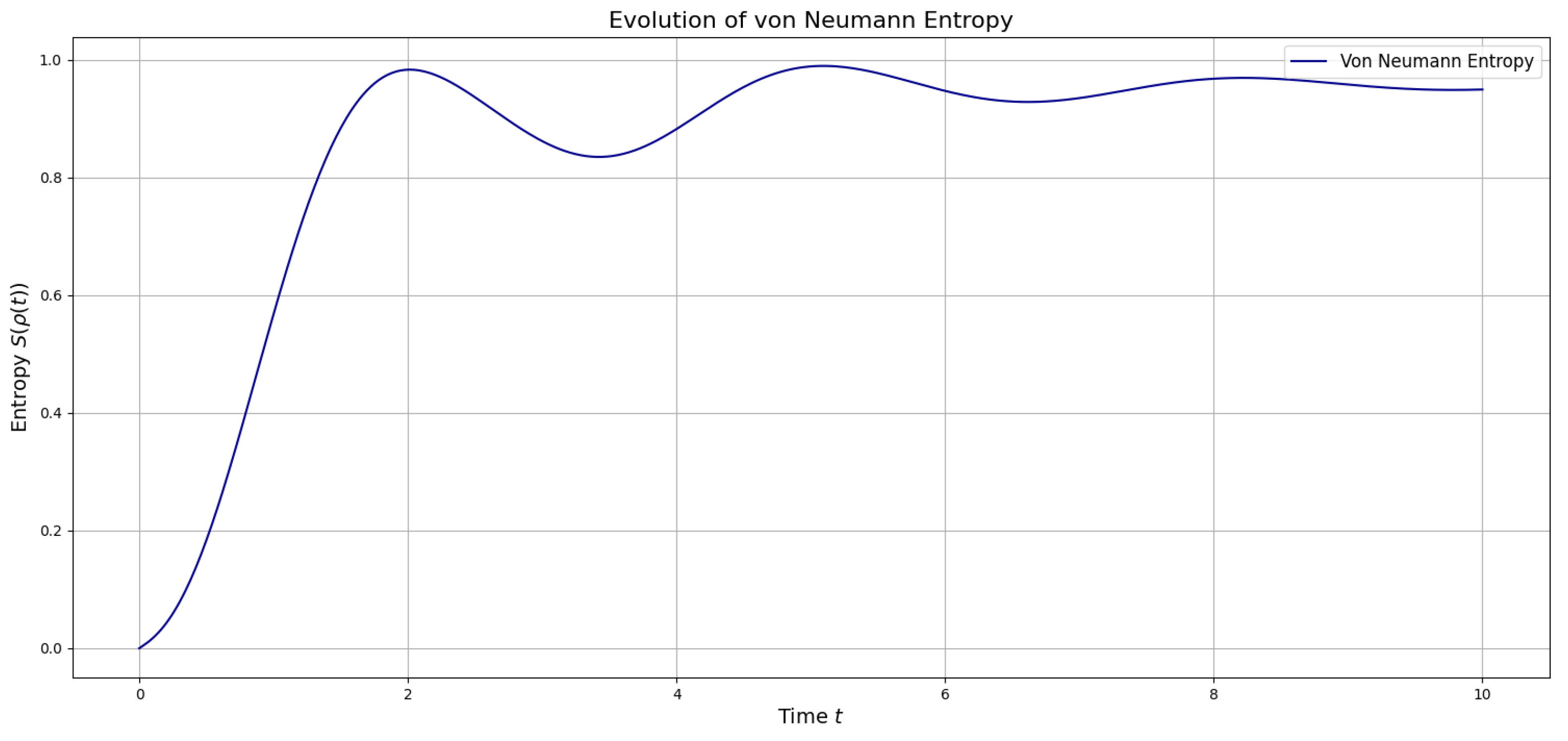
The damped oscillations in the von Neumann entropy (Figure A1) show a qualitative resemblance to both the three-hump analytical solutions of the GKSL equation derived from single-parameter approach (see equation (A5)). The plot in Figure A1 shows familiarities with the Rabi oscillations reported by Pla et al. [23]. However, the dissipative nature of our GKSL model implies that a direct comparison to the purely coherent Rabi oscillations in [23] requires careful consideration and is better termed as “damped Rabi oscillations”. This model may thus provide insights into spin-fraction evolution under damped electromagnetic perturbation in single atoms, but further analysis is warranted experimentally.
Appendix A.2. Analytical Expressions of a Pure and Stable Point on the Bloch Sphere: as Initial Condition
We now seek to obtain an analytical solution using an admissible point, , which lies on the quarter circle on the Northern hemisphere of the Bloch sphere, between singularities (see Section 3.9). This gives the following state:
which is in density matrix form:
We have system of ODEs from above which we solve with MATLAB, using as initial condition:
The final analytical expression results as:
Appendix A.2.1. Properties of the Analytical Solution on the Bloch Sphere
The analytical solution given above maintains exact Hermiticity through the conjugate relationship , with all imaginary components in the transient terms canceling exactly (data not shown for limitation purposes). Trace preservation emerges naturally via , where the diagonal elements’ time dependence guarantees unit trace for all . Moreover, the solution approaches the non-equilibrium steady state
which yields a preservation of quantum coherence through non-vanishing off-diagonal elements. This reflects the balance between the unitary evolution frequency and the dissipative decay rate (the same as for the solution in (A5)). The transient dynamics is governed by oscillatory terms and , exponentially damped by , while the initial coherence determines both the transient behavior and the properties of the steady state. We note that the steady state density matrix given in (A13) is Hermitian and has unit trace and it is positive semi-definite, hence satisfying the necessary requirements for a solution in open quantum systems.
The steady state in (A13) is now visualized on the Bloch sphere (Figure A2). The plot shows that this is a mixed state of very low purity, being close to the center of the Bloch sphere (pure states are on the surface of the sphere).
Figure A2.
Steady state in (A13) of the analytical solution on the Bloch sphere (A12), derived by solving the system of equations (49) with the initial conditions from the Bloch parametrization in (A10). Final steady-state bloch state-vector: .
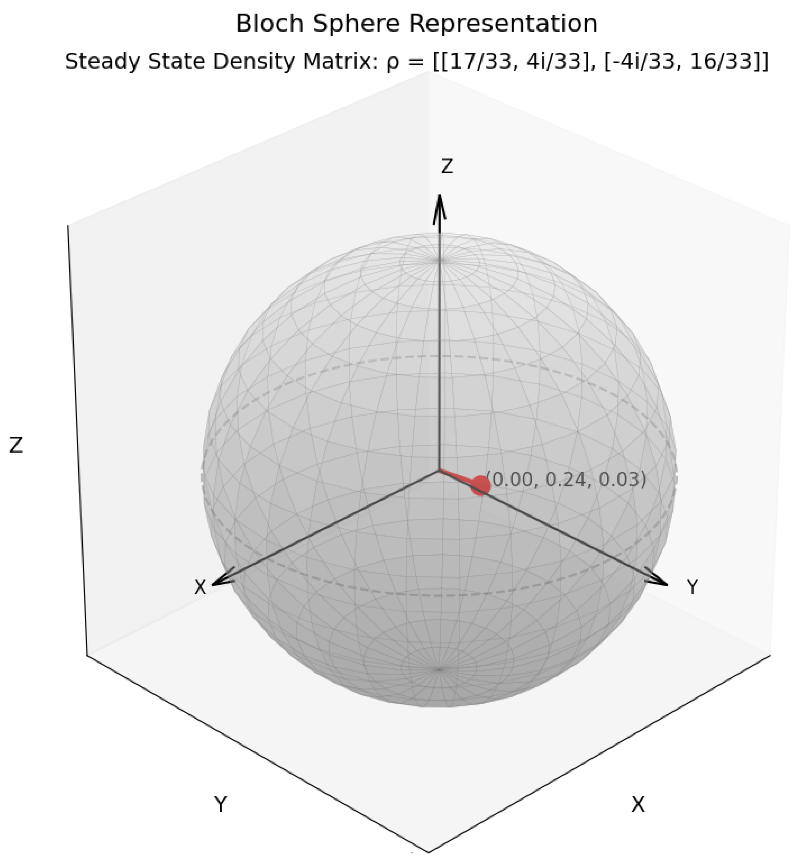
The Bloch vector (Figure A2) represents a quantum state with purity , exhibiting partial coherence, displaying slightly unequal populations in computational basis states ( and ). The non-zero y-component with magnitude indicates moderate quantum superposition, while its location well inside the Bloch sphere (Bloch vector length ) confirms it cannot be represented by a pure-state vector. This state exhibits significant mixedness with modest coherence, making it relevant for quantum information theory as it represents a typical steady state that might arise in open quantum systems subject to decoherence and dissipation processes. The density matrix for this steady state displays a similar von Neumann entropy of the analytical solution in (A12) as the previous state in (A5).
Figure A3.
von Neumann entropy evolution of the analytical solution in (A12) to the GKSL equation in (41) under the camel-like framework, with the initial conditions in (A10).
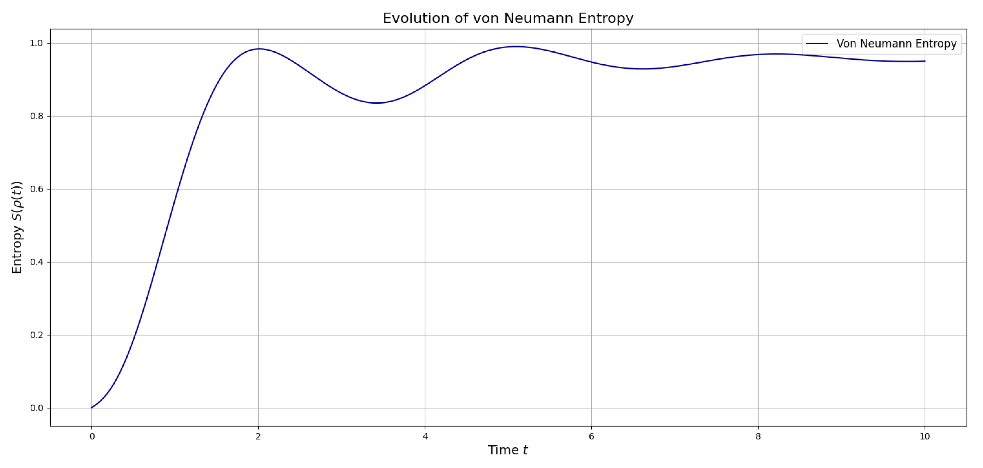
The entropy evolution in Figure A3 shows oscillations similar to those found in the single-parametrization approach (Section A.1). While these oscillations resemble Rabi oscillations, they differ crucially in their decay to a steady state, a hallmark of open quantum systems, unlike the undamped Rabi oscillations reported by Pla et al. [23]. This damped oscillatory behavior finds parallels in other physical systems, such as neutrino oscillations (exhibiting decaying sinusoidal patterns due to interactions and detection limitations) and neutral kaon () oscillations (where damping arises from kaon decay) [45].
Appendix A.3. Analytical Expressions of a Metastable Point by Bloch Parameter (θ,ϕ)=(0.05,0) as Initial Condition
In this final section, we shall derive the analytic expression of a metastable point belonging to the basin in the Bloch sphere, reported in the topological analysis section. The quantum state corresponding to is
which we calculate in density matrix form to:
We then use the same system of ODEs as for the other initial states,
which we solve using MATLAB code with (A15) as initial conditions.
We obtain:
We analyse the entropy evolution of this analytical solution in Figure A4.
The von Neumann entropy plot reveals the evolution of our quantum state under the specified dynamics, starting from a nearly pure state () in basin , reaching maximum mixedness () at , and eventually returning to purity. This behavior reflects the specific trajectory determined by our differential equations, showing substantial mixing before eventual purification. States initialized in exhibit prolonged dwelling times before eventually finding escape channels toward their final attractors, making them physically significant for quantum information processing. This topological obstruction creates effective barriers in the quantum state space, allowing for the existence of these metastable states that remain coherent for extended periods despite being energetically unfavorable, a property that emerges naturally from the gradient flow structure we analyzed.
The model of the metastable state has a entropy behavior that is experiencing something akin to quantum recurrences or resonances, but with very precise returns to pure states in between periods of mixing. Such behavior would be extremely difficult to realize in natural physical systems, as it requires highly controlled and isolated quantum dynamics that resist the typical irreversible decoherence processes, therefore we can conclude that metastable state in the respective topological basin do not reflect sound physical phenomena.
Figure A4.
Evolution of the von Neumann entropy for a quantum state initialized in the stable basin . The system begins in a nearly pure state (entropy ), reaches maximum mixedness (entropy ) at , and eventually returns to purity. This behavior demonstrates the characteristic dynamics of states in the basin, showing temporary confinement followed by escape to the final attractor. The non-monotonic entropy evolution reflects the topological structure of the gradient flow defined by the GKSL master equation.
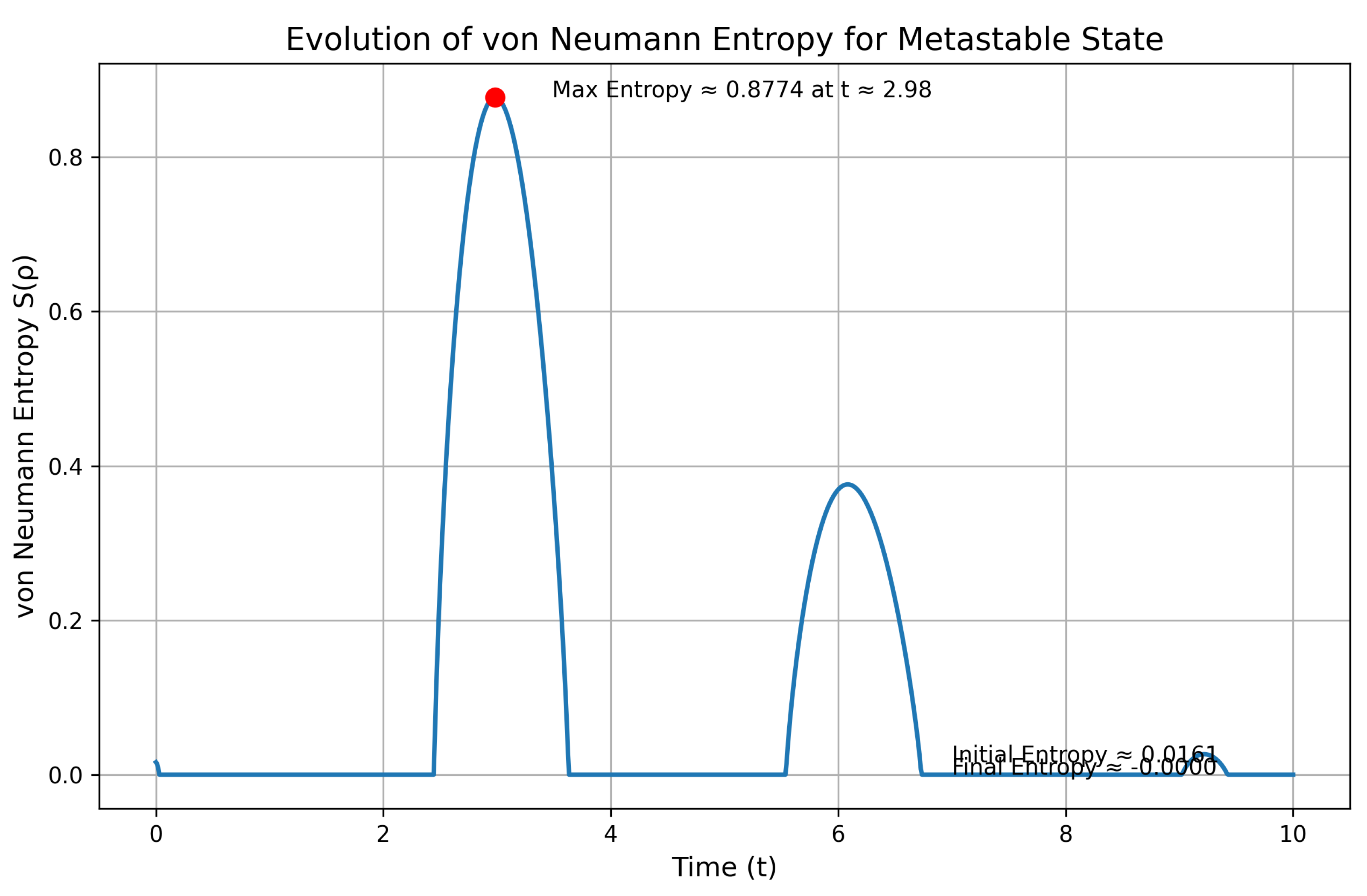
References
- Breuer, H.P.; Petruccione, F. The Theory of Open Quantum Systems; Oxford University Press: Oxford, 2002. [Google Scholar]
- Basieva, I.; Khrennikov, A. “What is life?”: Open quantum systems approach. Open Systems & Information Dynamics 2022, 29, 2250016. [Google Scholar] [CrossRef]
- Sun, H.B.; Milburn, G.J. Quantum open-systems approach to current noise in resonant tunneling junctions. Physical Review B 1999, 59, 10748. [Google Scholar] [CrossRef]
- Breuer, H.P.; Petruccione, F. The Theory of Open Quantum Systems; Oxford University Press: Oxford, 2002. [Google Scholar]
- Isar, A.; Sandulescu, A.; Scutaru, H.; Stefanescu, E.; Scheid, W. Open quantum systems. International Journal of Modern Physics E 1994, 3, 635–714. [Google Scholar] [CrossRef]
- Rivas, A.; Huelga, S.F. Open quantum systems; Vol. 10, Springer, 2012.
- Khrennikov, A. Open Systems, Quantum Probability, and Logic for Quantum-like Modeling in Biology, Cognition, and Decision-Making. Entropy 2023, 25, 886. [Google Scholar] [CrossRef] [PubMed]
- Wineland, D.J.; Monroe, C. Quantum decoherence and collapse of the wavefunction in a two-ion quantum system. Nature 1998, 392, 153–156. [Google Scholar] [CrossRef]
- Wineland, D.J. Experimental quantum optics. Proceedings of the National Academy of Sciences 2002, 99, 8225–8232. [Google Scholar]
- Haroche, S.; Raimond, J.M. Decoherence and the quantum-to-classical transition in cavity QED. Nature 2008, 452, 340–343. [Google Scholar] [CrossRef]
- Haroche, S.; Wineland, D.J. Nobel Prize in Physics 2012: Quantum control of atoms and photons. Science 2012, 337, 1055–1058. [Google Scholar]
- Khrennikov, A.; Basieva, I.; Pothos, E.M.; Yamato, I. Quantum probability in decision making from quantum information representation of neuronal states. Scientific reports 2018, 8, 16225. [Google Scholar] [CrossRef]
- Khrennikov, A.; Iryama, S.; Basieva, I.; Sato, K. Quantum-like environment adaptive model for creation of phenotype. BioSystems 2024, 242, 105261. [Google Scholar] [CrossRef]
- Plotnitsky, A.; Haven, E. The quantum-like revolution: A festschrift for andrei Khrennikov; Springer Nature, 2023.
- Khrennikov, A. Quantum-like modeling: From economics to social laser; Springer, 2020.
- Ingarden, R.; Kossakowski, A.; Ohya, M.; Ingarden, R.; Kossakowski, A.; Ohya, M. Information Dynamics. Information Dynamics and Open Systems: Classical and Quantum Approach.
- Lindblad, G. On the generators of quantum dynamical semigroups. Communications in Mathematical Physics 1976, 48, 119–130. [Google Scholar] [CrossRef]
- Lindblad, G. Cloning the quantum oscillator. Journal of Physics A: Mathematical and General 2000, 33, 5059. [Google Scholar] [CrossRef]
- Gorini, V.; Kossakowski, A.; Sudarshan, E.C.G. Completely positive dynamical semigroups of N-level systems. Journal of Mathematical Physics 1976, 17, 821–825. [Google Scholar] [CrossRef]
- Zur, H.; Garrison, J.C. Quantum open system dynamics. Journal of Mathematical Physics 2001, 42, 4711–4733. [Google Scholar]
- Khrennikov, A.Y. What is Life? Open Quantum Systems Approach. In Open Quantum Systems in Biology, Cognitive and Social Sciences; Springer, 2023; pp. 31–51.
- Rabi, I.I. Space Quantization in a Gyrating Magnetic Field. Phys. Rev. 1937, 51, 652–654. [Google Scholar] [CrossRef]
- Pla, J.J.; Tan, K.Y.; Dehollain, J.P.; Lim, W.H.; Morton, J.J.; Jamieson, D.N.; Dzurak, A.S.; Morello, A. A single-atom electron spin qubit in silicon. Nature 2012, 489, 541–545. [Google Scholar] [CrossRef]
- Warshel, A.; Kamerlin, S.C. Free-Energy Landscape of Enzyme Catalysis. Biochemistry 2008. [Google Scholar]
- Dobson, C.M. Protein folding and misfolding. Nature 2003, 426, 884–890. [Google Scholar] [CrossRef]
- Landau, L.D.; Lifshitz, E.M. Quantum Mechanics: Non-Relativistic Theory, 3rd ed.; Pergamon Press: Oxford, 1981. [Google Scholar]
- Manzetti, S. Spectral and Topological Dynamics of the GKSL Equation in the Camel-Like Framework: Non-Hermitian Effects and Entropy Oscillations on the Bloch Sphere., 2025.
- Press, W.H.; Teukolsky, S.A.; Vetterling, W.T.; Flannery, B.P. Numerical Recipes 3rd Edition: The Art of Scientific Computing; Cambridge University Press, 2007; pp. 899–905. Discussion of Forward Euler and other numerical integration methods.
- Johansson, J.R.; Nation, P.D.; Nori, F. QuTiP 2: A Python framework for the dynamics of open quantum systems. Computer Physics Communications 2013, 184, 1234–1240. [Google Scholar] [CrossRef]
- Breuer, H.P.; Laine, E.M.; Piilo, J.; Vacchini, B. Colloquium: Non-Markovian dynamics in open quantum systems. Reviews of Modern Physics 2016, 88, 021002. [Google Scholar] [CrossRef]
- Minganti, F.; Miranowicz, A.; Chhajlany, R.W.; Nori, F. Quantum exceptional points of non-Hermitian Hamiltonians and Liouvillians. Phys. Rev. A 2019, arXiv:quant-ph/1905.09448]100, 062131. [Google Scholar] [CrossRef]
- Abo, S.; Tulewicz, P.; Bartkiewicz, K.; Özdemir, Ş.K.; Miranowicz, A. Experimental Liouvillian exceptional points in a quantum system without Hamiltonian singularities. New Journal of Physics 2024, 26, 123032. [Google Scholar] [CrossRef]
- Kurian, P. Computational capacity of life in relation to the universe. Science Advances 2025, 11, eadt4623. [Google Scholar] [CrossRef] [PubMed]
- Nielsen, M.A.; Chuang, I.L. Quantum Computation and Quantum Information, 1st ed.; Cambridge University Press: Cambridge, 2000. [Google Scholar]
- Breuer, H.P.; Petruccione, F. The Theory of Open Quantum Systems; Oxford University Press, 2002.
- Zurek, W.H. Decoherence, einselection, and the quantum origins of the classical. Physics Today 2003, 44, 36–44. [Google Scholar] [CrossRef]
- Bengtsson, I.; Życzkowski, K. Geometry of quantum states: an introduction to quantum entanglement; Cambridge University Press, 2017.
- Zanardi, P.; Rasetti, M. Holonomic quantum computation. Physics Letters A 1999, 264, 94–99. [Google Scholar] [CrossRef]
- Sjöqvist, E.; Tong, D.M.; Nguyen, B.A.; Johansson, M.; Sjöqvist, E.; Andersson, L.M. Non-adiabatic holonomic quantum computation. New Journal of Physics 2012, 14, 103035. [Google Scholar] [CrossRef]
- Xu, G.F.; Zhang, J.; Tong, D.M.; Sjöqvist, E.; Kwek, L.C. Nonadiabatic Holonomic Quantum Computation in Decoherence-Free Subspaces. Physical Review Letters 2012, 109, 170501. [Google Scholar] [CrossRef]
- Schirmer, S.G.; Solomon, A.I. Quantum control landscapes and optimally robust control. Physical Review A 2010, 82, 022305. [Google Scholar]
- Berry, M. Optical vortices evolving from helicoidal integer and fractional phase steps. Journal of Optics A: Pure and Applied Optics 2004, 6, 259. [Google Scholar] [CrossRef]
- Bomzon, Z.; Kleiner, V.; Hasman, E. Space-variant Pancharatnam–Berry phase optical elements with computer-generated subwavelength gratings. Optics Letters 2002, 27, 1141–1143. [Google Scholar] [CrossRef]
- Wiseman, H.M.; Milburn, G.J. Quantum measurement and control; Cambridge University Press, 2010.
- Ashie, Y.; et al. . Evidence for an oscillatory signature in atmospheric neutrino oscillation. Physical Review Letters 2004, 93, 101801. [Google Scholar] [CrossRef] [PubMed]
Figure 1.
Entropy of the Bell states (top - overlappinng to one plot), the product states in (19) and (21) (middle), and the mixed states in (23) (with and ), calculated by the Lindbladian evolution in the GKSL framework given in [2] with . The simulation was initiated with all pairs of states entangled (not separated) at .
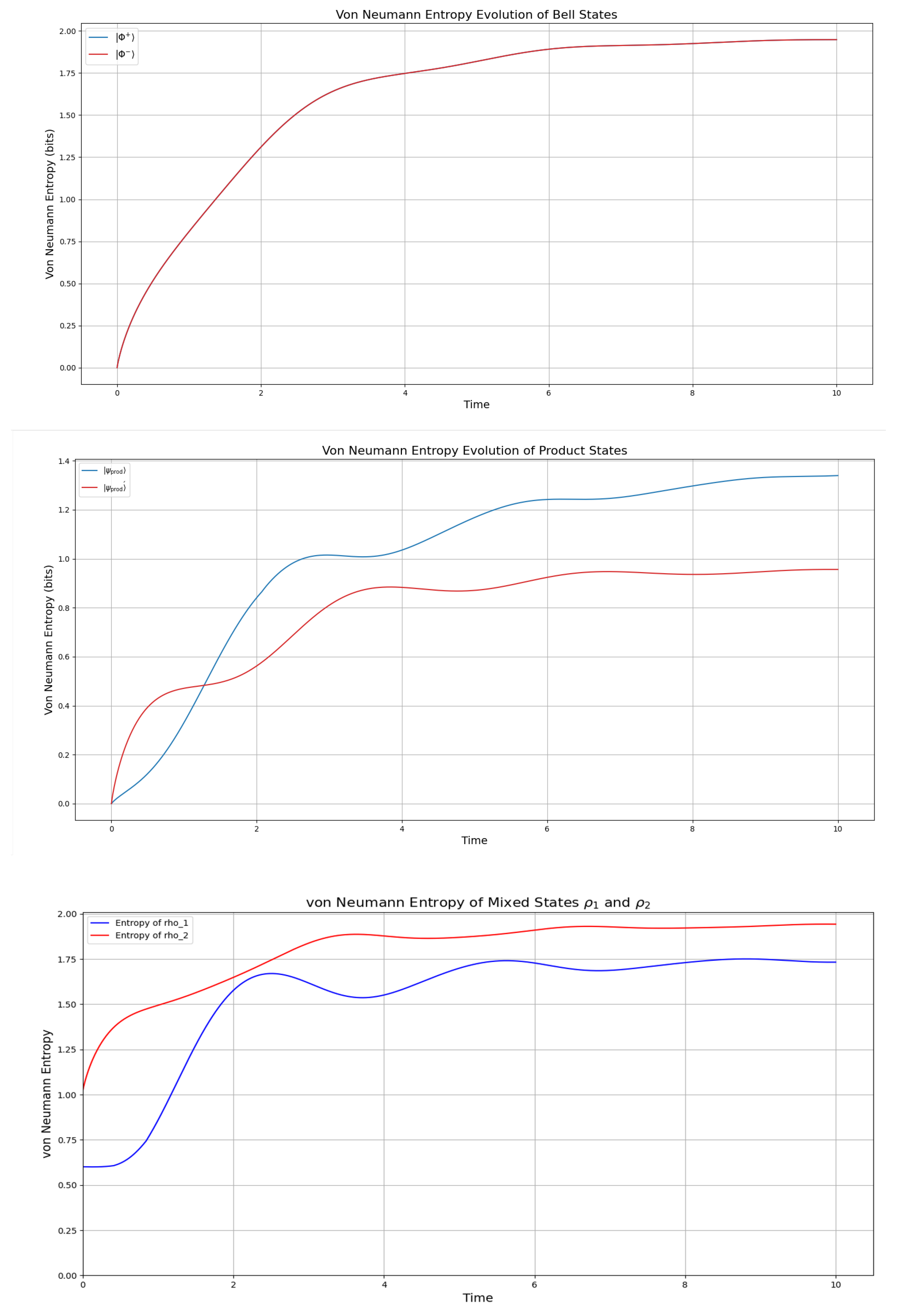
Figure 2.
Entropy evolution of the Bell-state calculated by the GKSL equation under the framework given in [2] with . x-axis: , y-axis: Time, z-axis: Entropy plot in red: Entropy of the system by the inflection point value of derived from the analysis by [27], corresponding to the equivalent plot in Figure 1 (Generated in Octave/Python) for optimal graphics. We plot only since is equal.
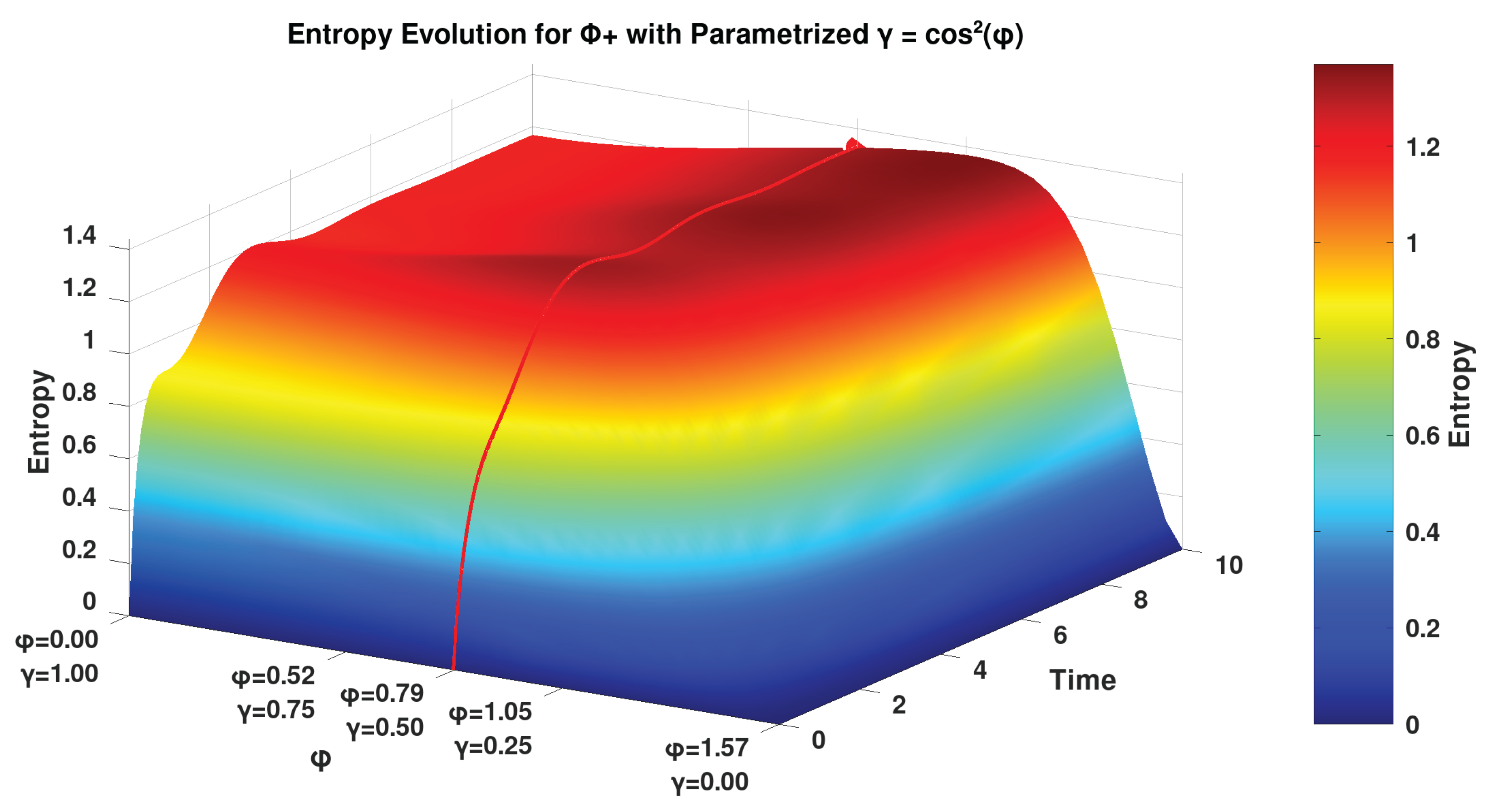
Figure 3.
Entanglement entropy of the Bell-states (which overlap to one plot) (top), the product states in (19) (middle), and the mixed states in (23) (with and ) (bottom), calculated by the Lindbladian evolution in the GKSL framework given in [2] with . The plots of the Bell-states overlap, while for the other states, it shows each individual reduced density matrix entropy under the GKSL evolution. The simulation was initiated with all pairs of states entangled (not separated) at .
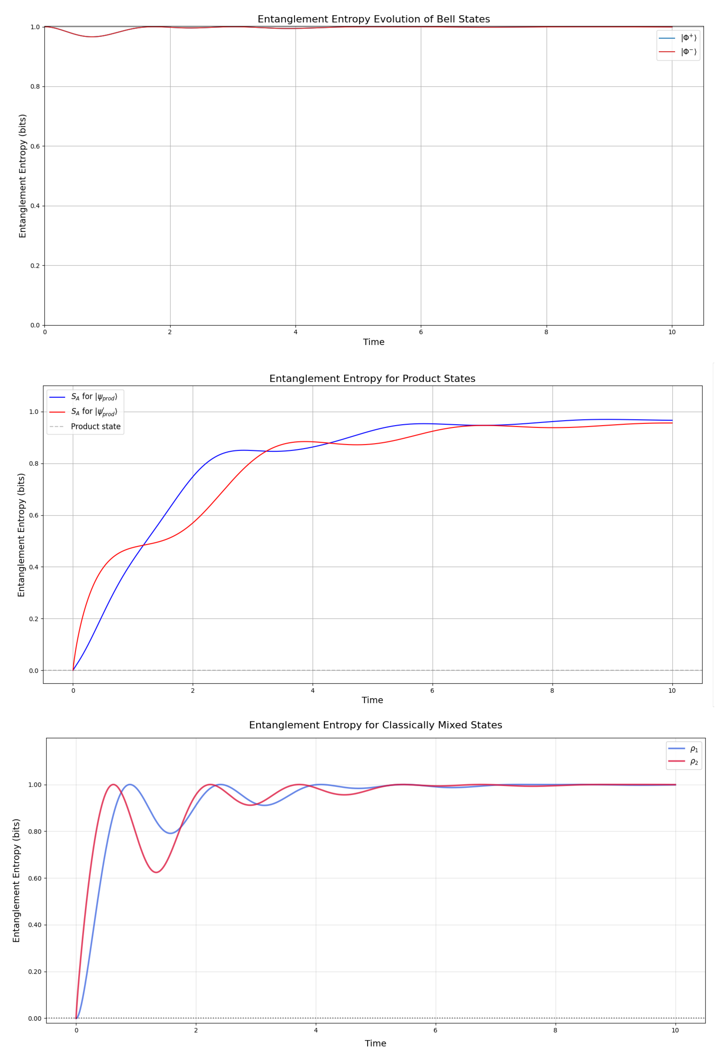
Figure 4.
Mutual information of the Bell-states (top - overlapping to one plot), the product states in (19) (middle), and the mixed states in (23) (with and ) (bottom), calculated by the Lindbladian evolution in the camel-like framework given in [2] with . The simulation was initiated with all pairs of states entangled (not separated) at . The mutual information is calculated by generating the entropy function using log2, as the mutual information is computed in bits (base-2 units), so it starts at 2 for maximally entangled states, as we see for the Bell-states. The mixed state starts at 0.8, since it is not entirely pure.
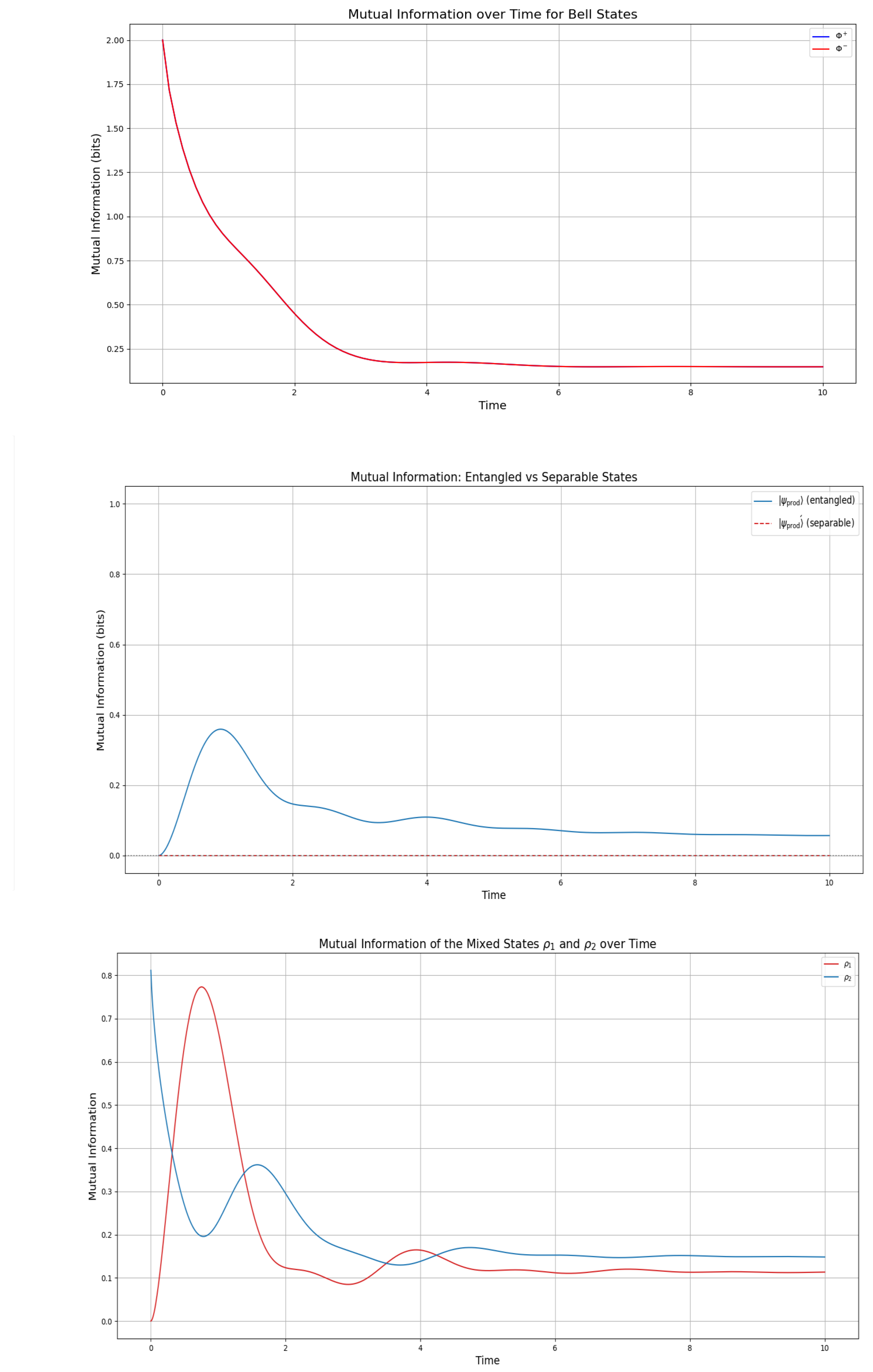
Figure 5.
Rate of information exchange for the Bell-states (top - overlapping to one plot) by the first derivative of the entanglement entropy, the product states in (19) (middle), and the mixed states (bottom) in (23) (with and ), calculated by the first derivative of the entanglement entropy, under the Lindbladian evolution with the camel-like behavior given in [2], with . The simulation was initiated with all pairs of states entangled (not separated) at .
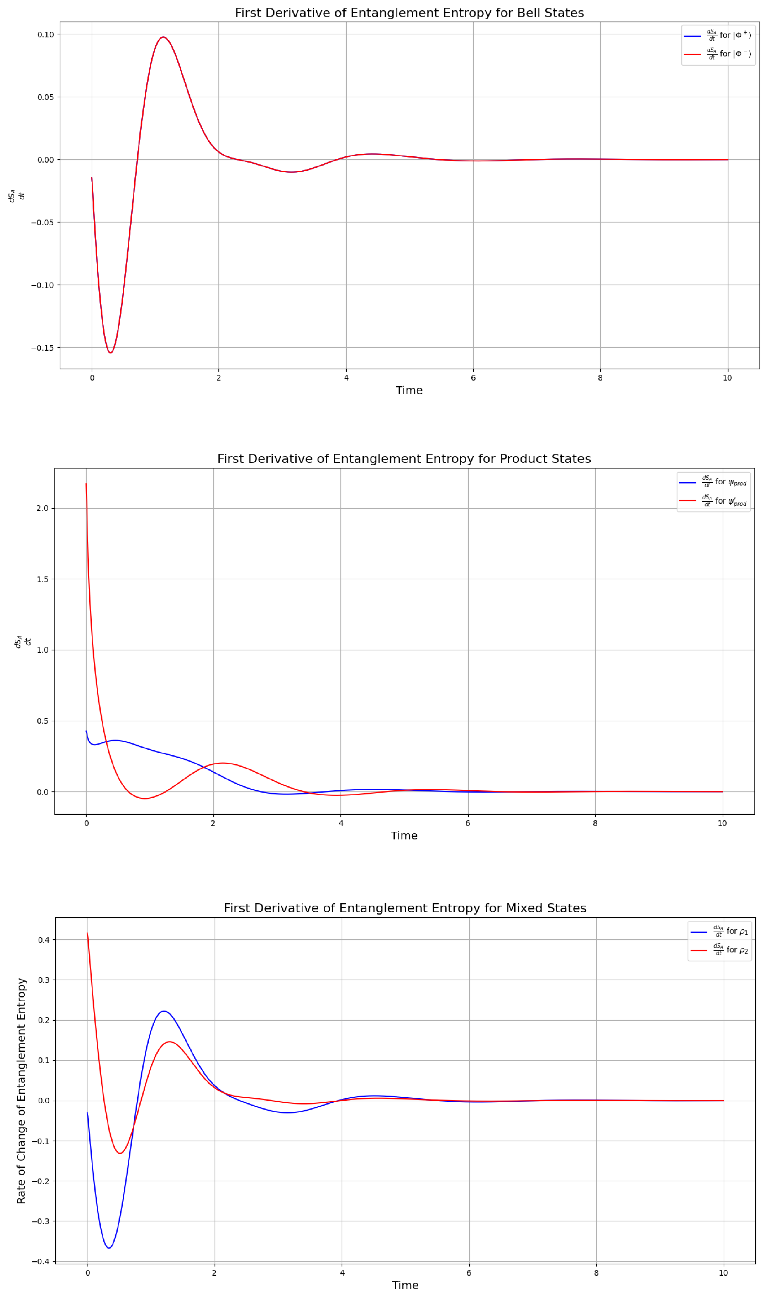
Figure 6.
Quantum discord of the states modeled by the Lindbladian evolution in the KB-picture [2], for the Bell states (top - overlapping to one plot), the product states in (19) (middle), and the mixed states in (23) (bottom) with and assigned as probabilities, with . The simulation was initiated with all pairs of states entangled (not separated) at .
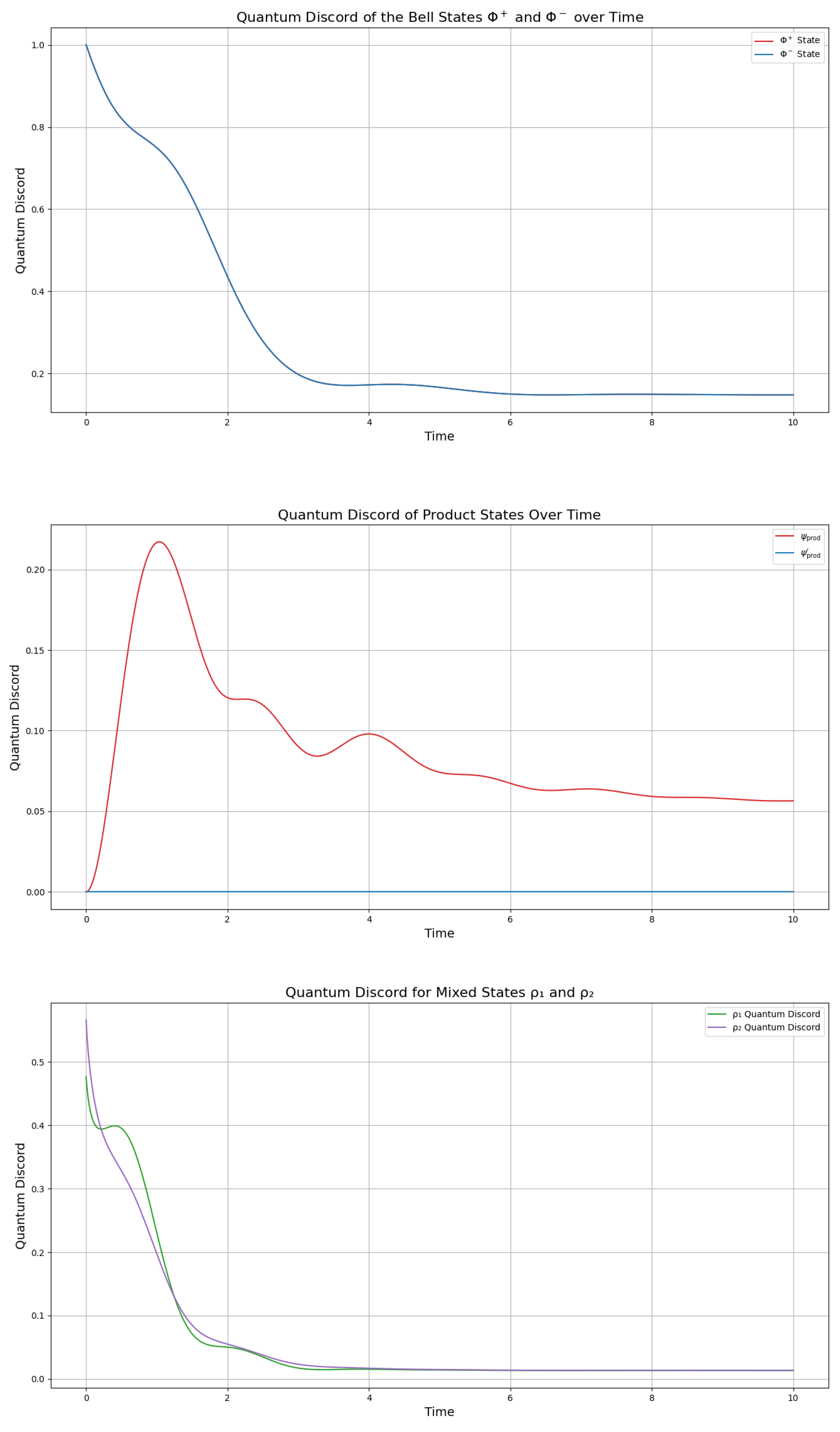
Figure 7.
Evolution of quantum steering by the CHSH parameter for the Bell states (top left), the product states in (19) (top right), and the mixed states in (23) (bottom) with and assigned as convexity coefficients. under the KB-picture [2]. The simulation was initiated with all pairs of states entangled (not separated) at .
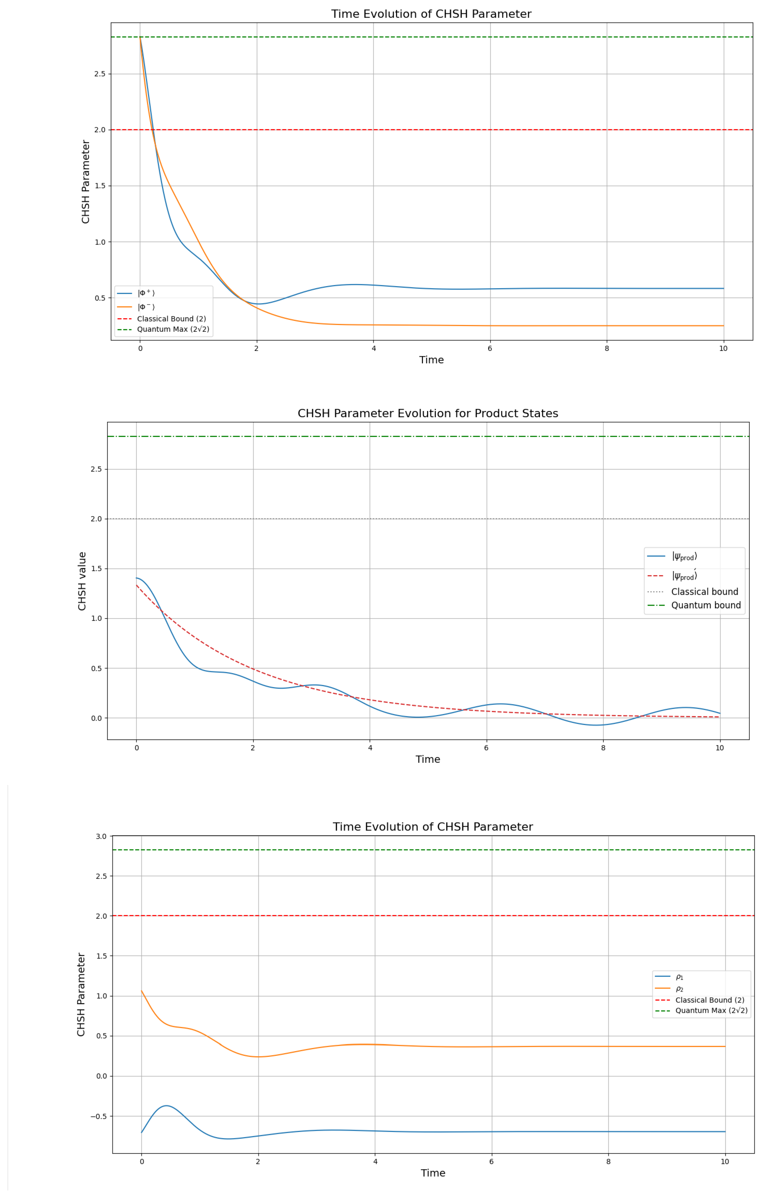
Figure 8.
Left: Entropy evolution; Right: Entanglement entropy evolution. System simulated by the parametrization of the convexity coefficients, for the mixed state , with . under the Khrennikov-picture [2]. Here we plot the entropy evolution for from equation (34). The case of is identical to , so it is omitted for graphical purposes. The simulation was initiated with all pairs of states entangled (not separated) at .
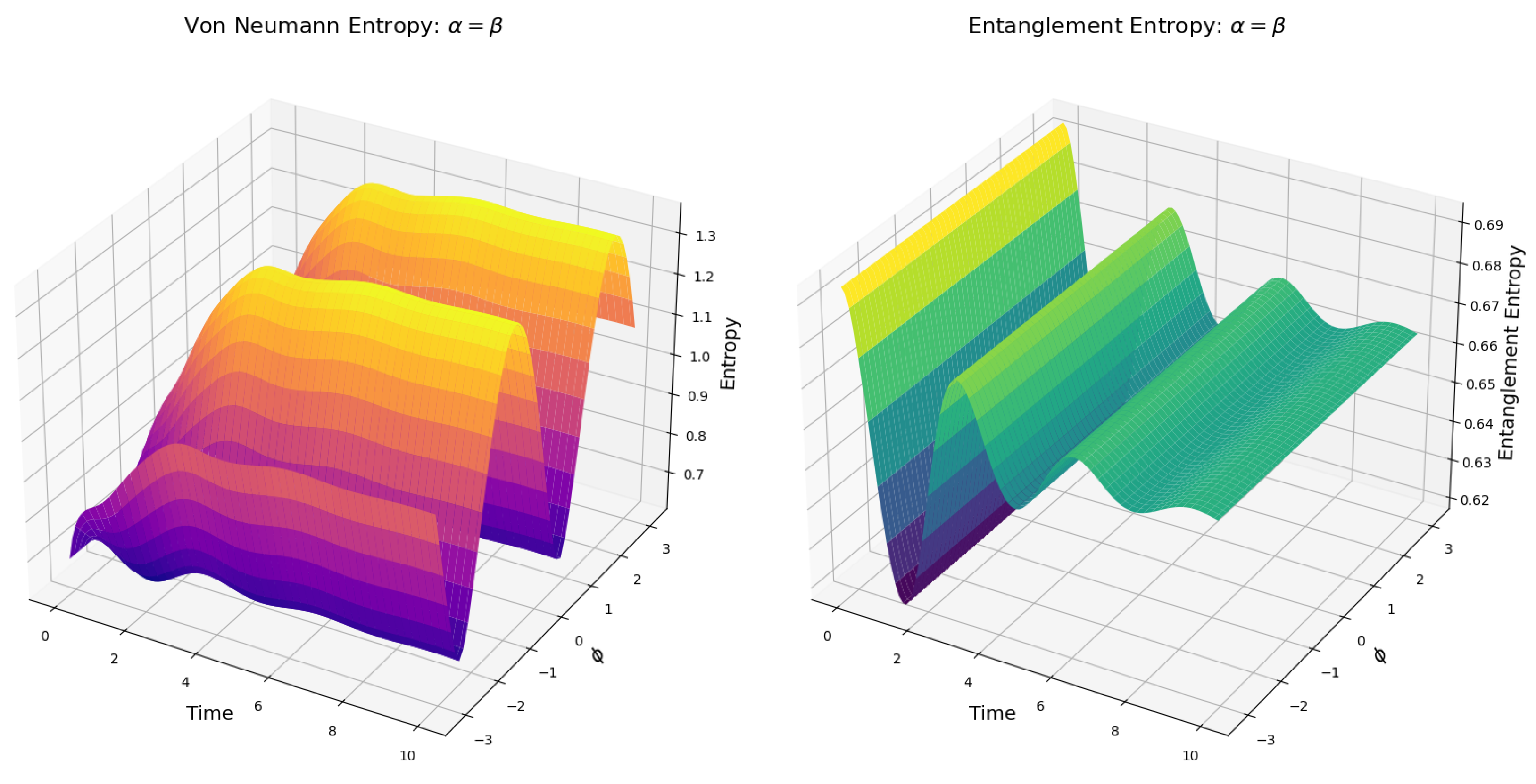
Figure 9.
Evolution of the von Neumann entropy of a superposition of pure states with respect to the parameter on the Bloch sphere in (52), under the GKSL equation in (49) within the camel-like framework.
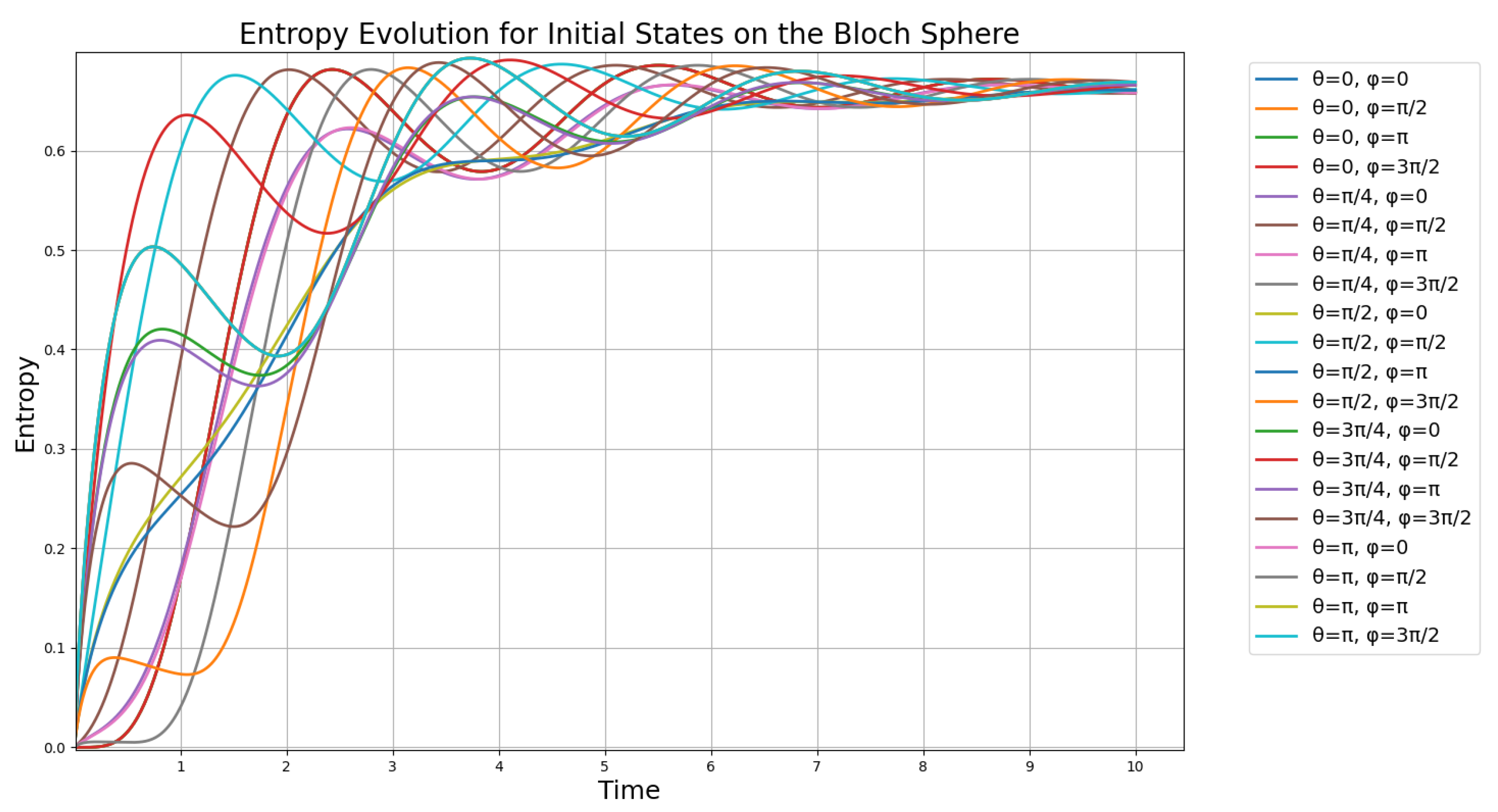
Figure 10.
Unstable states by the parameters and from the set in (53) represented on the Bloch sphere. The four unstable points at each quadrant intersection on the lower quarter circle are shown across the red circle belt. The South Pole state has multiplicity of 2 and is shown in azure, where both ) occur, forming six states visible as five decoherence-sensitive states.
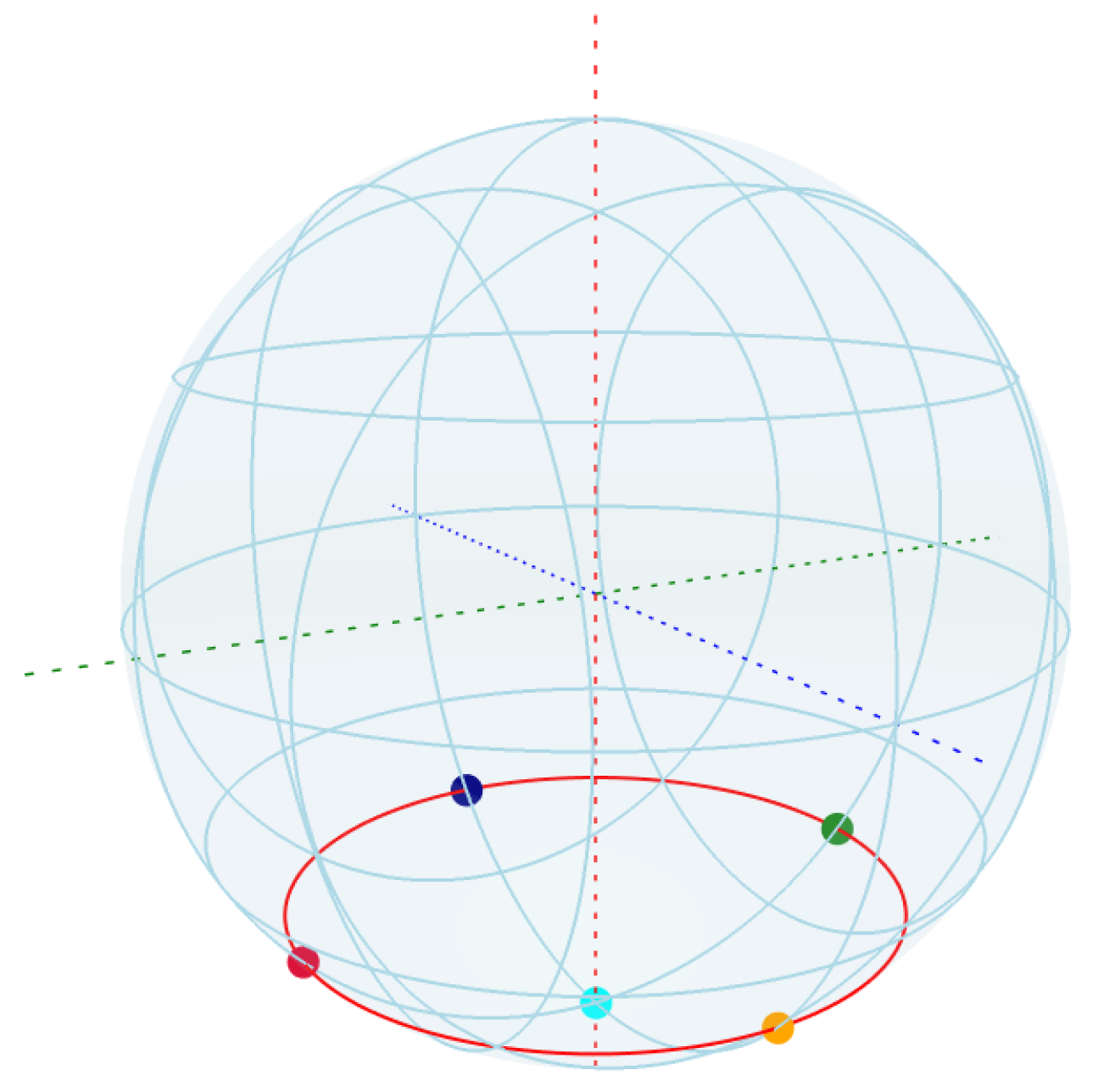
Figure 11.
The gradient flow of the Lyapunov function where and are defined in (70). Red points: Highly unstable points from the set defined in (53). The circle highlights the third quarter circle where states are highly unstable. White arrows indicate the gradient flow direction, while cyan lines show specific flow trajectories. Blue regions represent areas where is close to zero and where the states are unstable and decohere rapidly. Red regions represent areas where h has large values and where the inherent states are stable and do not decohere rapidly. All states on the surface have maximal purity, being on on the Bloch sphere.
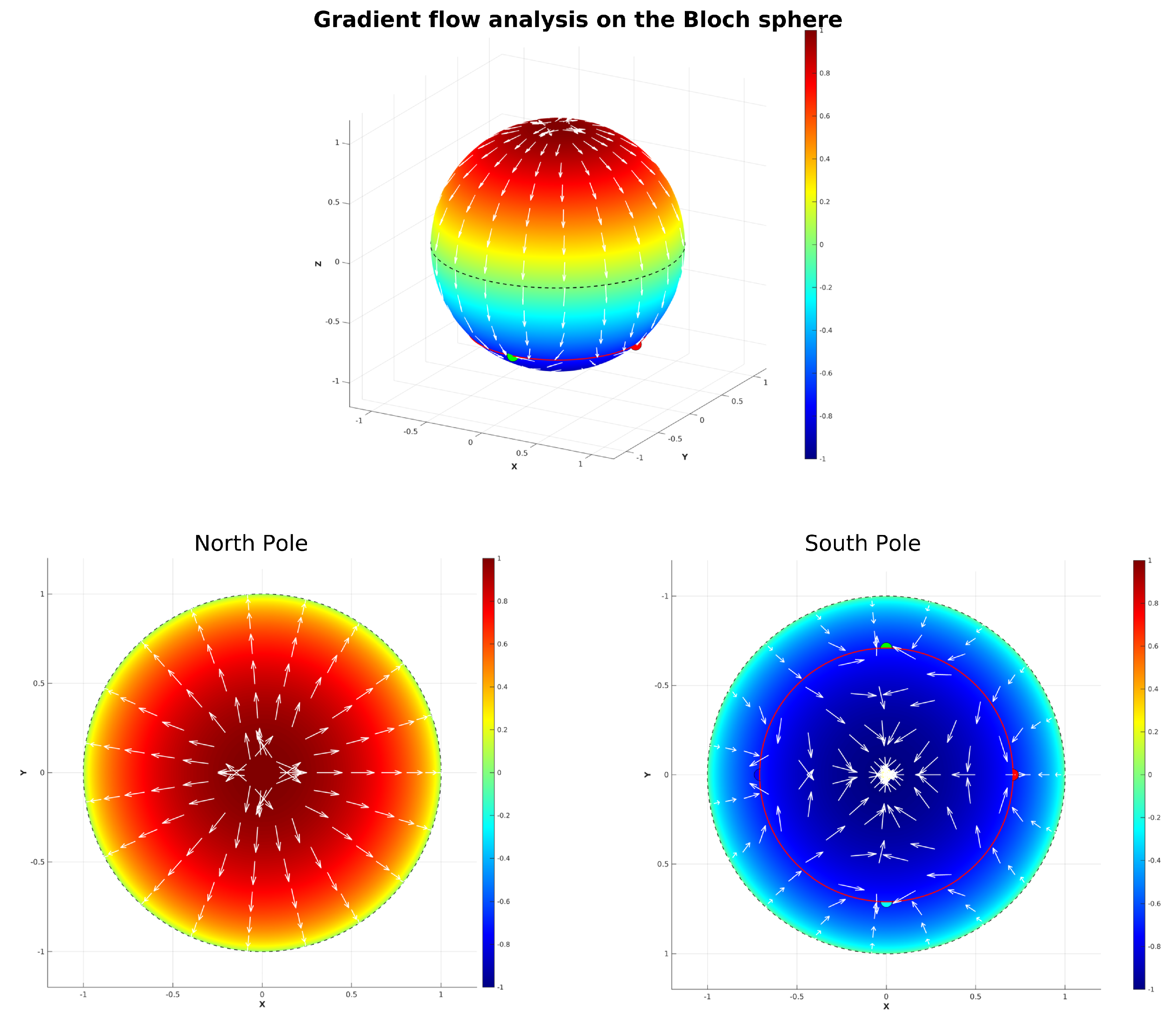
Figure 12.
The Bloch sphere colored by basin classification from the gradient flow analysis. The blue regions contains stable states that evolve towards meta-states, in the southward direction. The red region contains stable and metastable states that evolve towards the South Pole, crossing the third quarter circle.
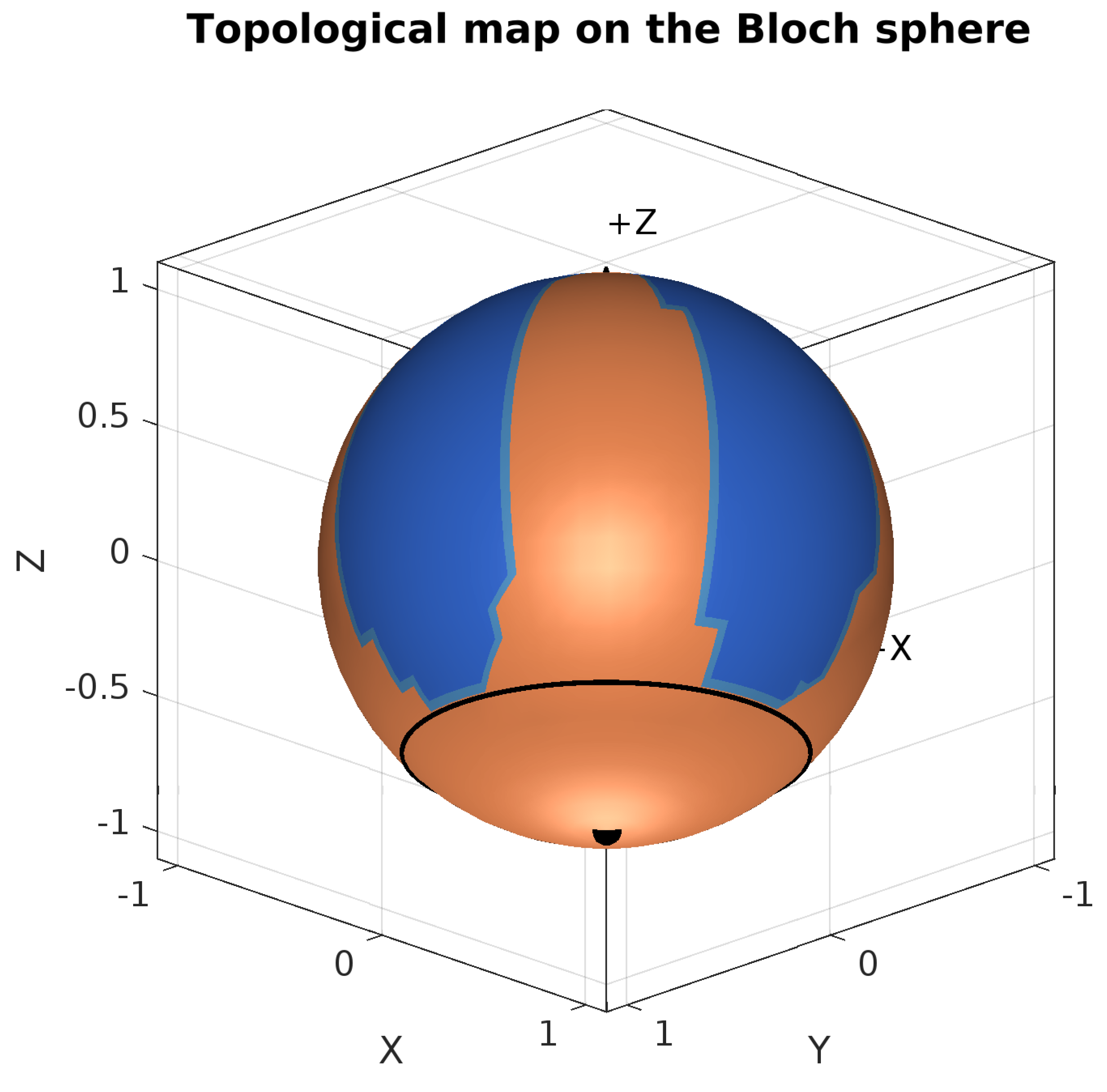
Figure 13.
Evolution of quantum states on the Bloch ball by purity. Upper half shows the paths on the Bloch ball from the surface (maximal purity) to the core (mixed states) of six different pure states evolving by the GKSL equation under the camel-like framework into a universal final mixed state. The final mixed state is the convergence steady state for all states on the Bloch sphere under the GKSL equation with the camel-like formalism.
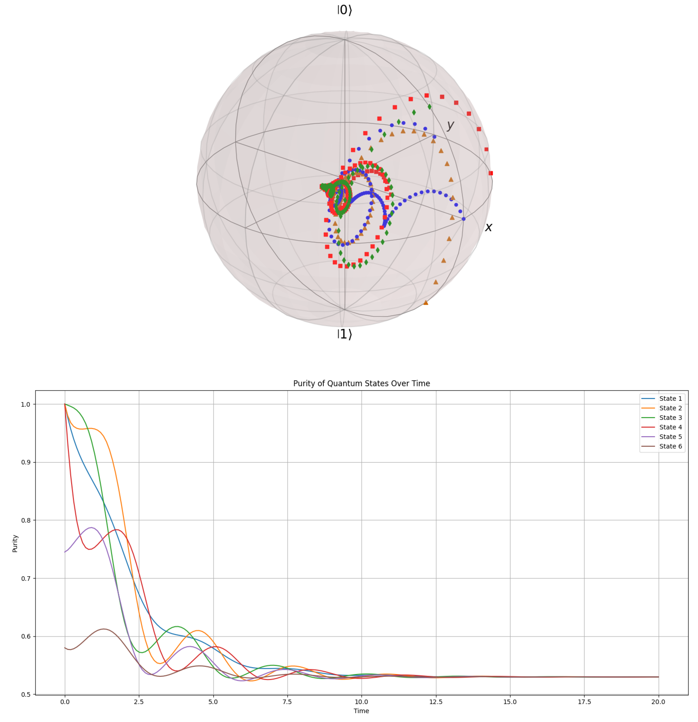
Disclaimer/Publisher’s Note: The statements, opinions and data contained in all publications are solely those of the individual author(s) and contributor(s) and not of MDPI and/or the editor(s). MDPI and/or the editor(s) disclaim responsibility for any injury to people or property resulting from any ideas, methods, instructions or products referred to in the content. |
© 2025 by the authors. Licensee MDPI, Basel, Switzerland. This article is an open access article distributed under the terms and conditions of the Creative Commons Attribution (CC BY) license (http://creativecommons.org/licenses/by/4.0/).
Copyright: This open access article is published under a Creative Commons CC BY 4.0 license, which permit the free download, distribution, and reuse, provided that the author and preprint are cited in any reuse.


