Submitted:
27 January 2025
Posted:
28 January 2025
You are already at the latest version
Abstract
Quantum computing, leveraging the principles of superposition and entanglement, speeds up the computational process in dynamical systems. Quantum Phase Estimation (QPE) which is a core of many quantum algorithms is an oracle to determine a significant invariant of systems, namely the eigenvalues of the state transition matrix. In addition to showing the scalability of QPE, this paper illustrates the time evolution of phase in the Schrödinger’s equation through Python Code executed in the Qiskit/Aer simulator. In addition, this paper proposes an efficient method for phase estimation of a non-self-adjoint Hamiltonian, which offers great potential in solving complex quantum systems.
Keywords:
Quantum Phase Estimation (QPE)
; Non-self-adjoint Hamiltonian
; Schrödinger’s equation
; Quantum computing
1. Introduction
This paper demonstrates the potential of the scalable QPE algorithm to capture time evolution of the phase derived by Schrödinger’s equation. Notably, this paper introduces a novel method for phase estimation when we are dealing with a non-self-adjoint Hamiltonian. This innovation holds the dimension of the original Hamiltonian unchanged and brings significant promises for tackling intricated quantum systems. We begin by reviewing essential concepts such as modal decomposition in quantum computations, Quantum Fourier Transform (QFT) required to implement QPE, and the inherent probabilistic nature of quantum measurement described by von Neumann measurement.
Quantum computers have the potential to revolutionize and solve longstanding computational problems in cryptography, search, optimization, communication, and simulation of quantum systems [1,2,3]. Shor's algorithm for prime factorization [4,5], Grover’s algorithm for unstructured search [6], and the HHL algorithm [3], which is highly relevant to finite element method (FEM) in engineering, are a few notable quantum algorithms. However, unlike classical computing machines, quantum computer hardware is still nascent, and suffers for performing accurate computation of elementary arithmetic operations. Gehlot et al. [7] presented the quantum-classical architecture for solving linear differential equation using a proper encoding of an arbitrary state vector. Solving linear differential equations enables the simulation of the linear state observer discussed in [8] using Positive Operator Valued Measure (POVM) of a closed quantum system. The authors in [1] presented a table comparing the runtime of classical algorithms for Linear System Problem (LSP) against their quantum counterparts. They indicated that the number of operations required by the best classical algorithm, the Conjugate Gradient (CG) method, is higher than HHL, the slowest quantum algorithm.
The quantum Fourier transform is an efficient quantum algorithm for computing the Fourier transform and it is pivotal in the quantum phase estimation algorithm to estimate eigenvalues of a unitary operator. The development of QFT has been explained in detail in many studies such as [6,9,10]. These studies note that QFT generally does not accelerate the computation of the Fourier transform over classical methods. QFT is the basis for another quantum subroutine algorithm called quantum phase estimation. Briefly, in QPE, a word describing a binary fraction is encoded as the phase of the unitary operator. It is important to note that the length of the binary fraction adjusts to the desired accuracy of the estimated phase.
The role of phase estimation shows up when discussing the eigenvalues of a linear system. By reformulating a dynamical computational model into an eigenvalue problem, QPE has the potential to solve widespread and multi-domain problems. A quantum computational problem exploits QPE to extract eigenvalues of the observer associated with a physical system. References [9,11] discuss the detailed derivation of QFT for phase estimation. Moreover, they provided a detailed illustration of the steps to recover the phase of a unitary matrix using a single ancilla qubit circuit.
1.1. Eigenvalue
The mathematical framework of a huge number of physical problems ends up with either Ordinary Differential Equations (ODE) or linear system problems. For instance, the governing equations of mechanical systems typically result in an ODE or a Partial Differential Equations (PDE) model that live in the field of reals. On the other hand, Schrödinger’s equations, that describe the dynamics and quantum probability for a closed system, result in linear ODE equations that reside in complex field. Besides, Finite Element Models (FEM), that form the basis of today’s engineering problems, ultimately result in solving large scale systems of linear equations. Diagonalization is a practical approach to solve these problems. In the quantum paradigm, the state sits in the separable Hibert space , meaning that any arbitrary vector state can be written in orthonormal bases [12,13,14].
Let’s consider a self-adjoint matrix . There exist orthonormal eigenvectors associated with eigenvalues such that where is reserved for the dimension of matrix . Suppose linear systems can be written as , after writing matrix and vector in orthonormal bases, this problem can be rearranged as [3]. For example, consider the first order time-invariant (LTI) system like . The solution would be , where matrix is an self-adjoint matrix and is the initial states at time . It can be written as using quantum computing notation. This shows that diagonalization (modal decomposition), a typical method to solve challenging computational problems, is an approach used extensively in quantum computing.
1.2. Measurement and Simulation
According to the postulates of quantum mechanics, the time evolution of a closed quantum system is described by a unitary operator (here, is the phase), which preserves the norm of the state vector and ensures that quantum processes are reversible in principle [9,13,14,15].
Measurement in quantum mechanics, specifically the von Neumann measurement (also known as projective measurement), describes the process by which observing a quantum system causes its state to collapse onto one of the eigenvalues of the measured observable. Quantum measurement presents a unique challenge. There exists an ensemble of the realizations of the system under the identical set of conditions leading to the preparation of a single quantum mechanical system. Therefore, what is measured is the expected value of the observable [15]:
where is a state and and are the eigenvector of the observable and the quantum probability at which the system collapses, respectively. addresses that if system sits at state , measurement leads to one of the eigenvalues of the matrix .
1.3. Dynamics of Quantum Particles
The Schrödinger’s equation for a closed system (i.e., a system that does not exchange energy with the environment) is described by
where is a self-adjoint Hamiltonian of the system indicating the total energy of the system. The self-adjoint operator ensures that the energy eigenvalues are real, is Plank’s constant, and represents the quantum state vector belonging to Hilbert space . Schrödinger’s equation describes how a quantum state evolves over time in a closed system. Given an initial state and the Hamiltonian, the equation determines the future states of the system. The solution of this linear Schrödinger’s equation is
where is the initial state of the system at time .
If the system is not closed, it will interact with the surrounding thermal bath, and additional terms will be present in the equation describing the evolution of the state over time. One representation is the Lindblad master equation [14], which contains additional perturbation terms with a Hamiltonian representing the environment and plays an important role in diverse fields such as quantum optics and quantum information. However, in this paper, we only deal with closed systems.
Time Discretization
Digital quantum computers operate as discrete, digital computation machines. Consequently, to implement qubit dynamics in a quantum circuit, we must discretize the qubit's Ordinary Differential Equation (ODE). Sample time is defined as . Under these conditions, we can derive the discrete time model of the qubit dynamics as
where indicates time at step . This model allows us to represent the continuous evolution of the qubit state in discrete time steps, which is essential for digital quantum computation. The resulting discrete time model provides a framework for simulating and controlling qubit behavior in quantum circuits, bridging the gap between the continuous nature of quantum mechanics and the discrete operations of quantum computers (We assume = for simplicity and this does not impact any results presented in this paper).
1.4. Paper Organization
In section 2, we discuss quantum phase estimation and how to implement the phase kick-back algorithm for QPE in subsection 2.1. Subsection 2.2 addresses the post-processing needed to convert the output of the QPE quantum circuit into a phase in the decimal system, incorporating classical computations. Section 3 is dedicated to an illustrative example and simulation results. Before presenting the examples, subsection 3.1 defines the conventions for quantum computing operations in Qiskit. Subsection 3.2 contains a numerical example of QPE, demonstrating how to obtain the phase of a given matrix, besides demonstrating the scalability of the QPE algorithm, and perform post-processing for all phases of the given matrix. Additionally, we present a histogram related to all estimated phases of the example. Section 4 focuses on validating and verifying the results obtained by QPE, including the derivation of phases implementable through classical computation. The next section covers the time evolution of the Schrödinger equation with a self-adjoint Hamiltonian, explaining the phase at different time steps of the given Hamiltonian in the Schrödinger equation. So far, all discussions have been about self-adjoint Hamiltonians. In section 6, we propose an efficient method to handle QPE for a non-self-adjoint Hamiltonian. In contrast to the HHL algorithm, which doubles the dimensionality, this method operates with the original dimension of the Hamiltonian matrix. The final section is the conclusion and future work.
2. Quantum Phase Estimation Algorithm with a Self-Adjoint Hamiltonian
Phase estimation is widely applied to address a range of problems, including hidden subgroup identification, graph isomorphism, quantum walk analysis, quantum sampling, adiabatic computing, order finding, and large number factorization. The implementation of QPE has been described in numerous studies [11,16,17]. This widespread adoption and continuous refinement underscore QPE's status as a cornerstone technique in the field of quantum computation. Following section is dedicated to extract the phase of the unitary operator:
Here, is a unitary operator with complex eigenvalues of magnitude . The parameter is known as the phase which is supposed to be extracted by the phase kick-back algorithm below. Since this exponential function is periodic, its magnitude is .
2.1. Phase Kick-Back Algorithm for QPE for Self-Adjoint Hamiltonian
Figure 1 shows quantum circuit behind the QPE algorithm. Here, quantum registers initiate with state with vector representation as . The number of these ancilla qubits determines the accuracy of the estimated phase. To represent in binary fraction, the phase would be , where is the binary digit that can be either or . In other words, determines the number of the binary digits in estimated phase, . Last qubits, represented by , carry the eigenvector associated with the unitary operator . If and the dimension of the unitary operator is , then qubits are required to represent the state in the circuit. A Hadamard unitary gate takes each state of ancilla qubit to its superposition state, which can be interpreted as a representation in the frequency basis. Then, there is a controlled unitary gate, shown as , , and so on, on the way of each qubit which generates the associated binary digit. The Inverse Quantum Fourier Transform (IQFT) then processes this kicked-back phase to produce the final estimation. The term 'phase kick-back' is often associated with this QPE algorithm because the controlled-U operations 'kick back' the phase information onto the ancilla qubits. It should be mentioned that represents the controlled rotation matrix
where is inverse of the controlled rotation matrix.
It is important to note that the qubits representing the phase are ordered from least to most significant, with being the least significant qubit and being the most significant qubit. In other words, is the first digit number after the decimal point in binary representation of and is the farthest digit from decimal point.
2.2. Post Processing
The result of executing the QPE circuit, for the of runs, produces a histogram plot which illustrates the probability distribution of all possible measured states. The next step is to convert the highest probable state from binary representation to decimal system to interpret the results. The binary representation converts to a decimal value as follows:
The decimal value representation of the phase falls within the range .
3. Example and Simulation Results
QASM, the quantum simulator provided by Qiskit (an opensource software), paves the way to run a quantum algorithm on the local computer. Simulator at the level of circuit governed by quantum computation rules lets us verify the correctness of quantum code and quantum circuit behavior without needing to access the actual quantum hardware. In simulation each shot, which collapse at the state indicating eigenvalue of the observer, represents a single realization of the quantum system [18,19].
When working with quantum circuit notation, it is important to carefully consider Qiskit’s operational sequence against the standard matrix multiplication order. In quantum computing, operations on qubits are represented by unitary matrices, and the order in which these matrices are multiplied can significantly affect the final state of the qubits. Therefore, understanding the convention Qiskit uses for this multiplication is essential for constructing and simulating quantum circuits correctly. This ensures that our theoretical calculations and the actual implementation in Qiskit are consistent. The following subsection delves into the specifics of this order convention. It explains how Qiskit sequences operations and how this affects the resulting state of the quantum system.
3.1. Convention in Qiskit to Find Significant Qubits
We use two circuits, as shown in Figure 2, to illustrate the order of operations for both sequential application and tensor products of logic gates in Qiskit.
Figure 2a shows a quantum circuit containing two unitary logic gates: a Hadamard gate and an X (NOT) gate. Knowing the matrix representations of both gates, we will implement the circuit in Qiskit to obtain the final state and simultaneously compute the product of the gate matrices manually. By comparing these two approaches, we can gain Qiskit insight into how Qiskit orders gate operation.
This analysis reveals that Qiskit implementation of sequential gate operations aligns with a right-to-left order of matrix multiplication. It means that the rightmost gate in the circuit is applied first.
The same procedure is applied to analyze the tensor product of quantum gates. We then compare Qiskit’s implementation with manual calculations for tensor products:
Here, we see that Qiskit’s implementation of the tensor product coincides with a down-to-up order of matrix multiplication. And therefore, when calculating the effect of tensor products of multiple gates, Qiskit applies the bottom-most gate first, followed by the gates above it in sequence.
3.2. Phase Estimation for Unitary Matrix
In this section, we present an example of quantum phase estimation for a unitary operator. Our implementation demonstrates the scalability of the QPE algorithm.
Since the given matrix is diagonal, we can show that the true values of the phases associated with a given unitary operator are and . Figure 3 depicts the execution of the QPE algorithm in Qiskit for a unitary operator, using ancilla qubits and total shots (or runs). The histogram in Figure 3a shows the probability distribution of the estimated first phase, . The most probable state is , with a probability of 1 (or shots out of total shots). Figure 3b illustrates the histogram plot of the second phase. The most probable state is state , with shots out of shots. The two histogram plots left, Figure 3c,d are estimating third and fourth phase with most probable state and , in order. It should be noted that the first two digits in the states labels on x-axis refer to the two qubits of the unitary operator’s eigenvector.
The next step in the QPE process is to interpret the obtained states and extract the corresponding phases. This requires post-processing using classical computing techniques. The results of the post-processing step are as follows:
In this step, the quantum circuit computed phases are compared to the previously provided true values to evaluate the accuracy of the QPE algorithm.
For completeness, the next section provides the expressions for obtaining the true values of phase using classical computing.
4. Classical Approach to Obtain Phase
Let's consider a unitary operator and its corresponding eigenvector . We can represent them as follows:
where is an matrix, and each represents an element of the matrix . indicates row of . The eigenvalue problem can be expressed as
Then, pick out any arbitrary row . Now, we can express the eigenvalue equation as:
This expression allows us to calculate the phase θ using any row of the unitary operator and the corresponding components of its eigenvector . Further, it provides a method to verify the results obtained from the quantum phase estimation algorithm using classical computation.
5. Time Evolution of Schrödinger’s Equation with Self-Adjoint Hamiltonian
For a closed system, we can derive a discrete-time version of the Schrödinger’s equation, which is particularly useful for numerical simulations. For a closed system, discrete version of Schrödinger’s equation (considering ℏ=1) can be expressed as
where an integer number is reserved for time step counter, representing the number of time steps that have passed since the initial state. As long as, Hamiltonian is Self-Adjoint, the time evolution operator is guaranteed to remain unitary . In the following, we provide a numerical example of time evolution of Schrödinger’s equation.
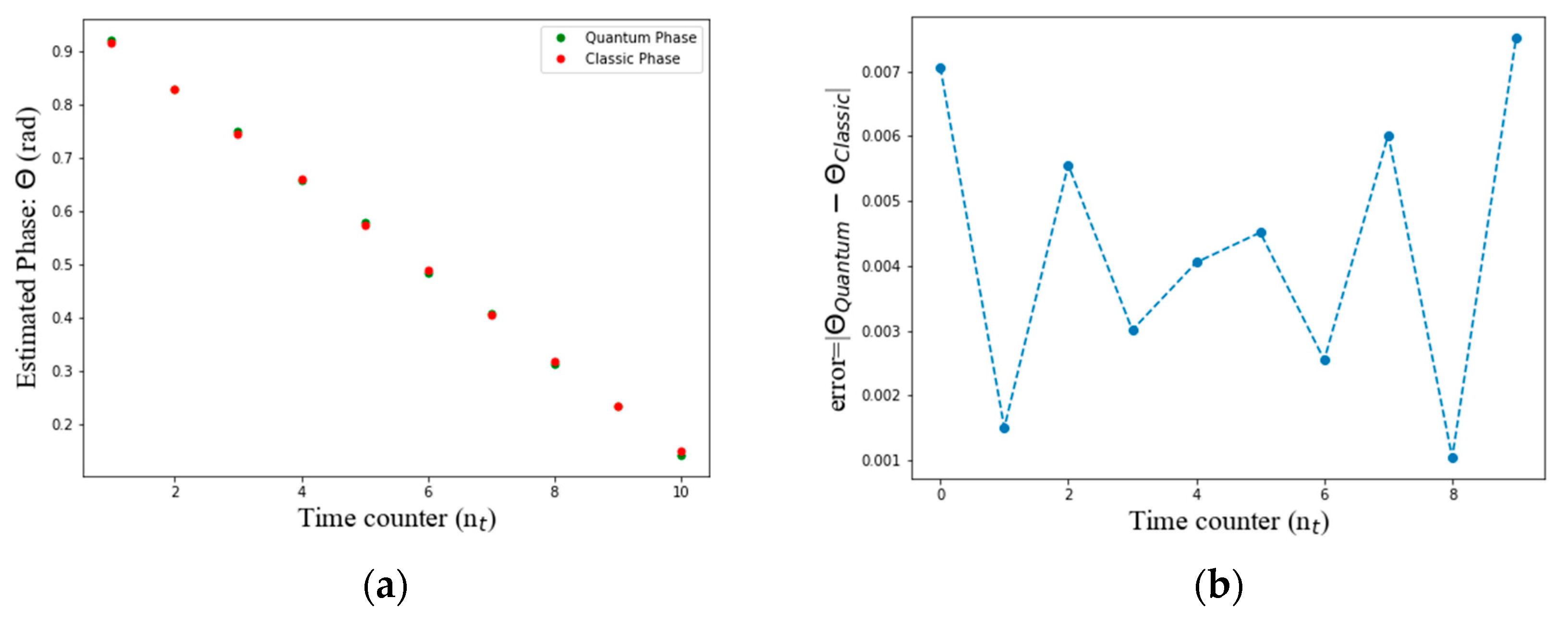
Consider a self-adjoint Hamiltonian , and a time step . By generating the unitary operator as at different time steps, first phases of the operator would be figure below.
Figure 4a illustrates the estimated phase of the Schrödinger operator over a series of time steps. It compares the phase evolution as calculated using both quantum and classical approaches. The x-axis represents the time steps, while the y-axis shows the phase values. This visualization helps in understanding how the phase evolves over time under different computational methods. Figure 4b depicts the difference between the phase estimates obtained through the quantum approach and those obtained through the classical approach. The x-axis represents the time steps, and the y-axis shows the difference in phase values. This plot is helpful in assessing the accuracy and reliability of the quantum method in comparison to the classical method and in highlighting any significant deviations between the two approaches.
6. Schrödinger’s Equation with Non-Self-Adjoint Hamiltonian
What if Hamiltonian is not self-adjoint? Can we still obtain its eigenvalue using quantum computation? In this section, we want to propose an efficient method to overcome this challenge. The decomposition of a non-self-adjoint matrix into the sum of two self-adjoint matrices can be expressed as
Consequently, the exponential of the matrix can be written as:
Horn et al. [20] demonstrated that for small time steps , we can approximate:
Since is self-adjoint, is a unitary operator and can be implemented into Quantum circuit for phase estimation. The problematic part of this decomposition lies in . This term is not unitary and therefore complicates its direct implementation in quantum circuit. Small tricks are key to overcome this challenge. Since diagonalization of both and yields similar structure, exponential of eigenvalue of multiply versus . Given this similarity, we can implement in another quantum circuit separately to eventually obtain the phase of matrix .
The last step is to correlate eigenvalues of the original non-self-adjoint matrix with decomposed matrices when the original matrix is normal (). If is normal, it is diagonalizable with a set of orthonormal eigenvectors [20]. We can substitute matrix with matrices and (Eq. (19.1)). It implies that and are both diagonal as expressed in Eq. Since and are self-adjoint, their eigenvalues would be real and we name them as and , eigenvalues of and respectively. Comparing Eq. and Eq results in Eq.
is reserved to a set of orthonormal eigenvectors of matrix . indicates a diagonal matrix filled with eigenvalues of matrix .
In contrast to the HHL algorithm, which requires converting a non-self-adjoint matrix into a self-adjoint matrix through stacking matrix and its conjugate transpose leading to doubling the dimension, this method doesn’t need any changes in dimension.
7. Conclusions and Future Work
In this study, we demonstrated the scalability of the QPE algorithm through the phase estimation of a 4×4 unitary operator. We also illustrated the time evolution of Schrödinger’s equation and proposed an efficient method for phase estimation of non-self-adjoint Hamiltonians without altering the dimension of the original matrix. Our future work will focus on exploring open systems and their environmental interactions as described by the Lindblad equation [14].
Author Contributions
Conceptualization, Mehrzad Soltani and Dr. Mark J. Balas; methodology, Mehrzad Soltani and Dr. Mark J. Balas; software, Mehrzad Soltani; validation, Mehrzad Soltani and Dr. Mark J. Balas; formal analysis, Mehrzad Soltani and Dr. Mark J. Balas; investigation, Mehrzad Soltani and Dr. Mark J. Balas; resources, Mehrzad Soltani and Dr. Mark J. Balas; data curation, Mehrzad Soltani and Dr. Mark J. Balas; writing—original draft preparation, Mehrzad Soltani; writing—review and editing, all authors; visualization, Mehrzad Soltani and Dr. Mark J. Balas; supervision, Dr. Mark J. Balas, Dr. Vinod Gehlot, Dr. Marco Quadrelli; project administration, Dr. Mark J. Balas; funding acquisition, Dr. Marco Quadrelli. All authors have read and agreed to the published version of the manuscript.
Funding
This research was funded by a contract with NASA Jet Propulsion Laboratory in 2024, maestro ID: M2300938.
Acknowledgements
Dr. Quadrelli and Dr. Gehlot’s contribution was carried out at the Jet Propulsion Laboratory, California Institute of Technology, under a contract with the National Aeronautics and Space Administration (80NM0018D0004), and Prof. Balas and Ms. Soltani’s contribution was carried out under a contract of Texas A&M University with JPL.
Conflicts of Interest
The authors declare no conflicts of interest.
Abbreviations
The following abbreviations are used in this manuscript:
| An arbitrary complex self-adjoint matrix (observer) | |
| A complex column vector | |
| ℂ | The set of complex numbers |
| Hamiltonian operator | |
| Hadamard quantum gate | |
| Hibert space | |
| The number of ancilla qubits to adjust the desired accuracy of the phase | |
| Dimension of the Hibert space | |
| ℕ | The set of positive integers |
| The number of qubits required to represent an eigenvector in binary system | |
| Time step counter in discrete-time simulation | |
| P,Q | Self-adjoint matrices derived from the decomposition of a non-self-adjoint matrix into the sum of two self-adjoint matrices can be expressed as |
| R | Controlled rotation quantum gate |
| t | Time |
| U | Unitary operator |
| v | Orthonormal eigenvectors |
| X | Pauli-X gate (Not gate) |
| x | Solution of linear systems of equations |
| |0⟩ | Ket 0, represented as the column vector |
| ⟨1| | Bra 1, represented as the row vector |
References
- Dervovic, D.; Herbste, M.; Mountney, P.; Severini, S.; Usher, N.; Wossnig, L. Quantum Linear Systems Algorithms: a Primer. Feb. 2018, [Online]. Available: http://arxiv.org/abs/1802.08227. 0822. [Google Scholar]
- Montanaro, A. Quantum algorithms: an overview. npj Quantum Inf. 2016, 2, 15023. [Google Scholar] [CrossRef]
- Harrow, A.W.; Hassidim, A.; Lloyd, S. Quantum Algorithm for Linear Systems of Equations. Phys. Rev. Lett. 2009, 103, 150502. [Google Scholar] [CrossRef] [PubMed]
- Yanofsky, N.S.; Mannucci, M.A. Quantum Computing for Computer Scientists; Cambridge University Press (CUP): Cambridge, United Kingdom, 2008. [Google Scholar]
- Young, P. , “Shor’s Algorithm for Period Finding on a Quantum Computer.” [Online]. Available: https://young.physics.ucsc.edu/150/period.pdf.
- Nielsen, M. A. and Isaac Chuang, L., Quantum Computation and Quantum Information. Cambridge University Press, 2011.
- Gehlot, V.P.; Balas, M.J.; Quadrelli, M.B.; Bandyopadhyay, S.; Bayard, D.S.; Rahmani, A. A Path to Solving Robotic Differential Equations Using Quantum Computing. J. Auton. Veh. Syst. 2022, 2, 1–9. [Google Scholar] [CrossRef]
- Clouatre, M.; Balas, M.; Gehlot, V.; Valasek, J. Linear Quantum State Observers. IEEE Trans. Quantum Eng. 2022, 3, 1–10. [Google Scholar] [CrossRef]
- Hundt, R. Quantum Computing for Programmers; Cambridge University Press (CUP): Cambridge, United Kingdom, 2022. [Google Scholar]
- Dell'Antonio, G. Lectures on the Mathematics of Quantum Mechanics I; Atlantis Press SARL: Paris, France, 2015. [Google Scholar]
- Mohammadbagherpoor, H. Experimental Challenges of Implementing Quantum Phase Estimation Algorithms on IBM Quantum Computer. Mar. 2019, [Online]. Available: http://arxiv.org/abs/1903.07605.
- Datta, N. Quantum Entropy and Quantum Information. Mathematical Statistical Physics 2006, 83, 395–466. [Google Scholar] [CrossRef]
- Breuer, H.-P. and Petruccione, F., The Theory of Open Quantum Systems. New York: Oxford University Press, 2003.
- Manzano, D. A short introduction to the Lindblad master equation. AIP Adv. 2020, 10, 025106. [Google Scholar] [CrossRef]
- Sontz, S.B. An Introductory Path to Quantum Theory: Using Mathematics to Understand the Ideas of Physics; Springer Nature: Dordrecht, GX, Netherlands, 2020. [Google Scholar] [CrossRef]
- Moore, A.J.; Wang, Y.; Hu, Z.; Kais, S.; Weiner, A.M. Statistical approach to quantum phase estimation. New J. Phys. 2021, 23, 113027. [Google Scholar] [CrossRef]
- Chiang, C.-F. Quantum Phase Estimation with an Arbitrary Number of Qubits. Int. J. Quantum Inf. 2013, 11. [Google Scholar] [CrossRef]
- Norlen, H. , Quantum Computing in Practice with Qiskit and IBM Quantum Experience. Packt Publishing, 2020.
- Tolotti, E.; Zardini, E.; Blanzieri, E.; Pastorello, D. Ensembles of quantum classifiers. Quantum Inf. Comput. 2024, 24, 181–209. [Google Scholar] [CrossRef]
- Horn, R.A.; Johnson, C.R. Topics in Matrix Analysis; Cambridge University Press (CUP): Cambridge, United Kingdom, 1991. [Google Scholar] [CrossRef]
Figure 1.
Quantum circuit associated with phase estimation of unitary operator U using phase kickback algorithm.
Figure 1.
Quantum circuit associated with phase estimation of unitary operator U using phase kickback algorithm.
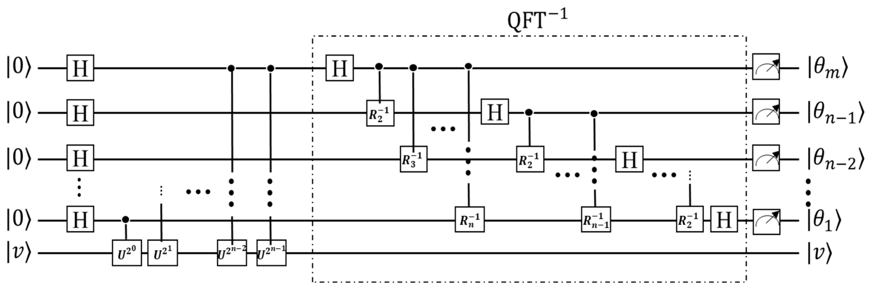
Figure 2.
The convention of operations in Qiskit; (a) Sequential product of two gates initiated with ; (b) Tensor product of two gates initiated with .
Figure 2.
The convention of operations in Qiskit; (a) Sequential product of two gates initiated with ; (b) Tensor product of two gates initiated with .
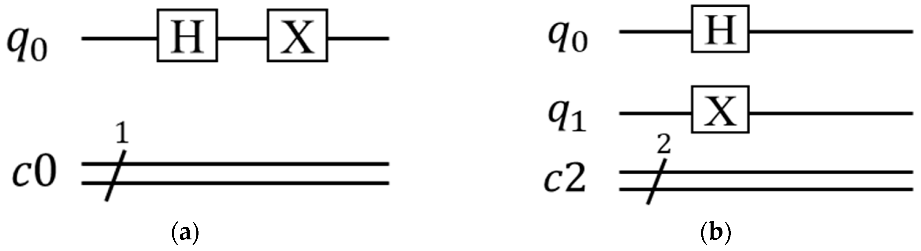
Figure 3.
Histogram of the estimated phases of the unitary operator introduced in Eq. (10) for 1024 shots; (a) First estimated phase ; (b) second estimated phase ; (c) Third estimated phase ; (d) Fourth estimated phase .
Figure 3.
Histogram of the estimated phases of the unitary operator introduced in Eq. (10) for 1024 shots; (a) First estimated phase ; (b) second estimated phase ; (c) Third estimated phase ; (d) Fourth estimated phase .
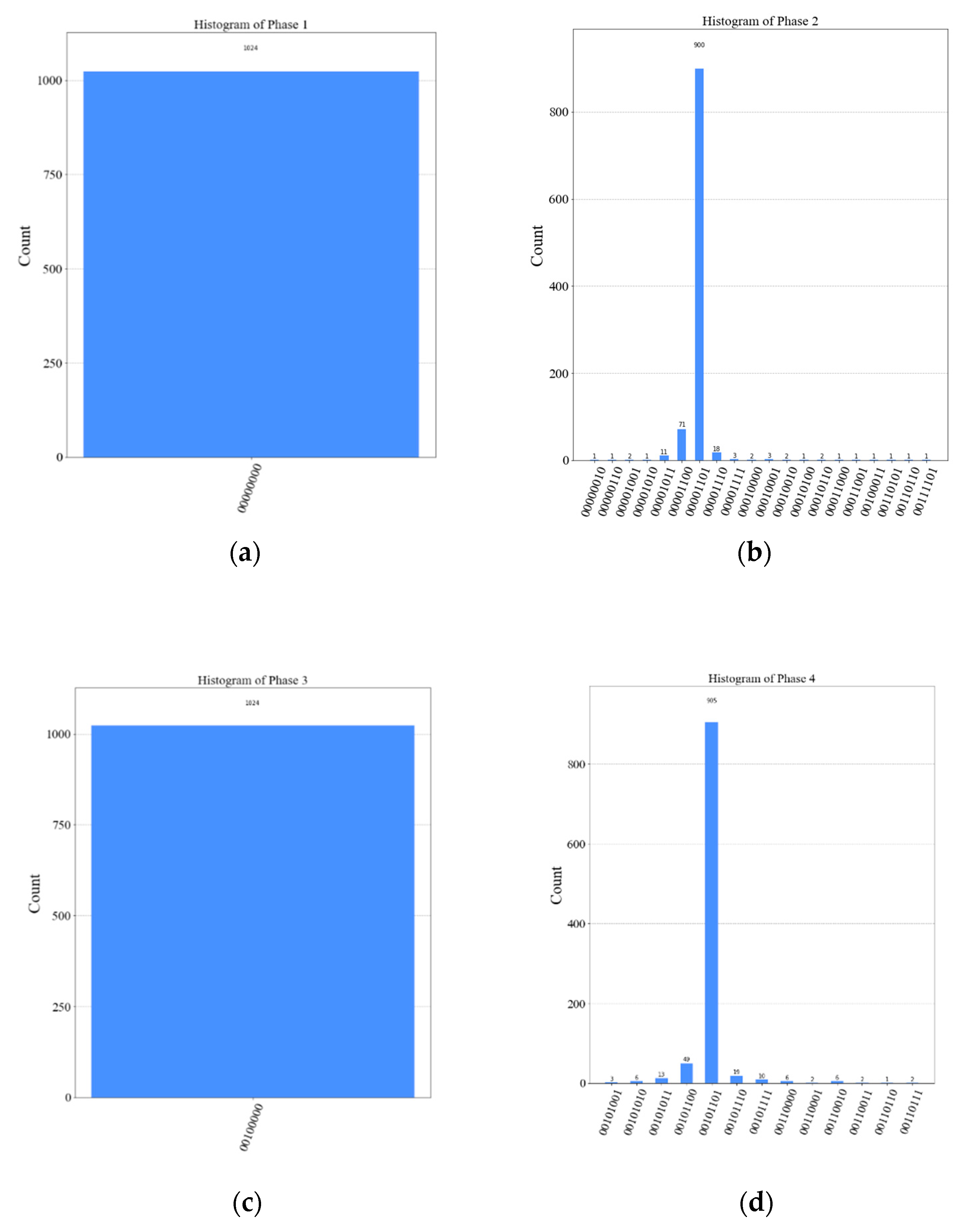
Figure 4.
Time evolution of the first phase of the Schrödinger Operator's phase; classical vs quantum approach; (a) Estimated phases at different time steps; (b) Difference between quantum and classical phase estimation methods.
Figure 4.
Time evolution of the first phase of the Schrödinger Operator's phase; classical vs quantum approach; (a) Estimated phases at different time steps; (b) Difference between quantum and classical phase estimation methods.
Disclaimer/Publisher’s Note: The statements, opinions and data contained in all publications are solely those of the individual author(s) and contributor(s) and not of MDPI and/or the editor(s). MDPI and/or the editor(s) disclaim responsibility for any injury to people or property resulting from any ideas, methods, instructions or products referred to in the content. |
© 2025 by the authors. Licensee MDPI, Basel, Switzerland. This article is an open access article distributed under the terms and conditions of the Creative Commons Attribution (CC BY) license (http://creativecommons.org/licenses/by/4.0/).
Copyright: This open access article is published under a Creative Commons CC BY 4.0 license, which permit the free download, distribution, and reuse, provided that the author and preprint are cited in any reuse.


