Submitted:
14 July 2025
Posted:
16 July 2025
You are already at the latest version
Abstract
Decoherence and the exponential scaling of Hilbert space are fundamental challenges for scalable quantum technologies. This work introduces Difference-Based Variational Reconstruction (DVR), a novel function-space control paradigm that addresses these challenges by enabling feedback directly in the operator domain. By expanding the density matrix in a complete orthonormal operator basis, DVR represents the quantum system's state evolution through observable-mode amplitudes. We demonstrate that this DVR coefficient hierarchy provides a complete coordinate system for quantum states in terms of observable moments, including all orders of correlations. We rigorously prove that the evolution of these coefficients under a Lindblad master equation is equivalent to Heisenberg-picture expectation dynamics. Furthermore, we show that the time trajectory of these coefficients defines a path in observable-moment space, which can be derived from a variational principle involving a real-valued action functional: \[ S[c]=\int_0^t \sum_\alpha \left(\frac{dc_\alpha}{ds} - \sum_\beta M_{\alpha\beta} c_\beta(s)\right)^2 ds. \] This real-action path integral formulation offers a powerful description of dissipative quantum dynamics, unifying the Heisenberg picture and statistical-mechanical path integral approaches within a single operator-algebraic framework. This unification provides a profound physical interpretation of DVR, establishing it not merely as a numerical method, but as a coordinate system on the full quantum observable hierarchy, enabling direct control and diagnostics compatible with the inherent complexities of open quantum systems
Keywords:
quantum control
; open quantum systems
; lindblad master equation
; mathematical physics
; variational methods
; operator algebras
1. Introduction
The realization of robust and scalable quantum technologies hinges on our ability to precisely control quantum systems while mitigating the detrimental effects of decoherence. Open quantum systems are commonly modeled using the Lindblad master equation [1], which generalizes unitary evolution to include environmental effects. For a comprehensive treatment of open quantum systems, see Breuer and Petruccione [2]. Traditional quantum control paradigms often operate within the Hilbert space formalism, where the state of an N-qubit system is described by a vector in a -dimensional complex space. This exponential scaling presents formidable challenges for both simulation and control as the number of qubits increases. Furthermore, the interaction of quantum systems with their environment leads to decoherence, transforming pure states into mixed states and necessitating a description via the density matrix, which lives in an even higher-dimensional operator space.
To circumvent these limitations, this work introduces a novel approach: Difference-Based Variational Reconstruction (DVR) applied in the operator domain. Inspired by the success of variational methods in classical physics (e.g., for plasma equilibrium reconstruction), DVR proposes to expand the quantum system’s density matrix not in the computational basis of Hilbert space, but in a complete, orthonormal basis of the operator space. The coefficients of this expansion directly correspond to the expectation values of physical observables (moments, correlations), providing a physically intuitive and complete representation of the quantum state.
The central hypothesis explored in this paper is that this DVR coefficient hierarchy offers a more fundamental and unifying perspective on quantum dynamics. We propose that by representing the quantum state through these observable moments, we can naturally bridge seemingly disparate formalisms of quantum mechanics: the Schrödinger picture (via density matrix evolution), the Heisenberg picture (via operator evolution), and even path integral formulations (typically associated with position-space trajectories). This unification is particularly powerful for open quantum systems, where the complexities of decoherence and dissipation are naturally accommodated within the operator-algebraic framework.
The remainder of this paper is structured as follows: Section 2 formally states the Observable Hierarchy Representation and Pathwise Evolution Theorem, outlining the key properties of the DVR coefficient representation. Section 3 provides a detailed mathematical proof for each part of the theorem. Section 4 presents numerical validation of the theoretical claims. Finally, Section 5 discusses the profound physical implications of this unification and its significance for the future of quantum control and diagnostics.
2. Observable Hierarchy Representation and Pathwise Evolution Theorem
Theorem 1
(Observable Hierarchy Representation and Pathwise Evolution Theorem). Let be a finite-dimensional Hilbert space, and let be an orthonormal basis of the operator space (where ) with respect to the Hilbert–Schmidt inner product, i.e., .
Then:
-
(Expansion)Every density matrix admits a unique expansionwhere the coefficients are given by the projection .
- (Moment Hierarchy)The full set of coefficients encodes all observable moments of the quantum system, including all orders of correlations.
-
(Pathwise Evolution Equation)The evolution of under a Markovian (Lindblad) master equationinduces a closed system of linear ordinary differential equations (ODEs) for :where M is a real matrix determined by the superoperator in the chosen operator basis.
-
(Heisenberg Equivalence)The Heisenberg picture evolution of observables yieldsmaking DVR coefficient evolution equivalent to Heisenberg-picture expectation dynamics.
- (Pathwise Action Formulation)The time trajectory defines a path in observable-moment space, which can be derived from avariational principleinvolving a real-valued action functional . This real-action functional defines apath integral formulation in observable-moment space, offering an equivalent description of the dynamics analogous to statistical-mechanical path integrals or Feynman–Vernon influence functional methods for dissipative quantum systems.
Corollary 1
(Feedback-Controlled DVR as a Special Case). If an explicit control term is introduced to enforce
then minimizing the action
yields an optimal control strategy in coefficient space. This controlled DVR evolution recovers the feedback slope-matching approach developed in our prior work on DVR-based quantum control.
Proof.
The DVR framework expresses the system evolution as . Introducing a control term G modifies this to . The variational principle generalizes to minimizing the modified action functional , penalizing deviations from the desired slope matching. This is precisely the strategy employed in our earlier work, where G is designed adaptively to stabilize selected DVR coefficients. Thus, the controlled DVR approach is a special case of the general variational path integral formulation. □
3. Proof
We will prove each point in order.
3.1. Proof of (1): Expansion
Let be a Hilbert–Schmidt orthonormal basis, meaning . Since is a finite-dimensional vector space (with dimension for a D-dimensional Hilbert space ), any operator admits a unique expansion in this basis:
To find the coefficients , we can take the Hilbert–Schmidt inner product of both sides with :
Thus, the coefficients are given by . This proves (1).
3.2. Proof of (2): Moment Hierarchy
By definition, the coefficients are the expectation values of the basis operators at time t:
If the chosen operator basis is constructed from products of elementary observables (e.g., Pauli strings for qubits, where ), then:
- Basis elements corresponding to single-body operators yield first moments (e.g., ).
- Basis elements corresponding to products of two operators yield two-point correlations (e.g., ).
- Higher-order basis elements yield higher-order moments and correlations.
Since the basis spans the entire operator space , any observable can be expressed as . Its expectation value is . Therefore, the full set of coefficients completely determines the expectation value of any observable, and thus fully describes the moment hierarchy of the state. This proves (2).
3.3. Proof of (3): Pathwise Evolution Equation
Assume the density matrix evolves according to a Markovian (Lindblad) master equation:
Substitute the expansion of from (1) into this equation:
Due to the linearity of the time derivative and the superoperator :
Since is a basis for , the action of on any basis operator can also be expanded in the same basis:
where are the elements of a real matrix M (assuming are chosen to be Hermitian or anti-Hermitian, and preserves Hermiticity). Substituting this back:
By the uniqueness of the basis expansion, the coefficients on both sides must be equal:
This is a closed linear system of ODEs for the coefficients . This proves (3).
3.4. Proof of (4): Heisenberg Equivalence
In the Heisenberg picture, the observables evolve in time according to the adjoint superoperator :
with formal solution . The expectation value of an observable at time t in the Schrödinger picture is . Using the cyclic property of the trace and the relation between and ():
This shows that the time evolution of is consistent with the Heisenberg picture. More directly, the expectation value of a Heisenberg operator with a fixed initial state is:
From the Schrödinger picture, we have . Therefore,
It is a known property that . Applying this with and :
Hence, the evolution of DVR coefficients is precisely the evolution of Heisenberg-picture expectation values. The matrix M in the Schrödinger equation for is the representation of in the dual basis. This proves (4).
3.5. Proof of (5): Pathwise Action Formulation
Consider the system of ODEs for the coefficients :
We can define a real-valued action functional on paths in observable-moment space:
Minimizing this action, , with respect to variations in directly imposes the ODEs as the Euler–Lagrange equations. This constitutes a variational principle for the dynamics in coefficient space.
Furthermore, a path integral formulation can be constructed using this real-valued action. This approach is analogous to the Feynman–Vernon influence functional method [3]. In statistical mechanics and for dissipative quantum systems, path integrals with real-valued actions are commonly used, where the probability of a path is weighted by . Such path integrals concentrate around the classical (ODE) trajectories in the continuum limit:
where is a functional Dirac delta. This contrasts with the standard Feynman path integral (), which is typically for unitary evolution in position or momentum space and leads to interference.
However, the Feynman–Vernon influence functional formalism describes open quantum systems via path integrals over the density matrix (or pairs of position paths). The DVR hierarchy, by resolving the density matrix into a finite-dimensional operator basis, provides a concrete realization of such a path integral in observable-moment space. The action functional derived here enforces the local evolution law for these moments. Thus, the time trajectory of DVR coefficients defines a path in observable-moment space, and the real-action functional provides a path integral formulation that is analogous to statistical-mechanical path integrals and directly applicable to dissipative quantum dynamics. This proves (5).
□
4. Numerical Validation: Equivalence of Formalisms
To numerically validate the theoretical claims of the Observable Hierarchy Representation and Pathwise Evolution Theorem, particularly points (3) and (4) regarding the equivalence of evolution formalisms, we perform a simulation of a single-qubit system undergoing both unitary and dissipative dynamics. The master equation is solved numerically using the QuTiP library [4].
The system is defined by a Hamiltonian and an amplitude damping Lindblad dissipator with a decay rate , represented by the jump operator . The initial state is chosen as the ground state . We track the expectation values of the four Pauli operators over time, which serve as our DVR coefficients .
We compare the time evolution of these coefficients obtained via three distinct methods:
- Schrödinger Picture (Density Matrix Evolution): The density matrix is evolved using QuTiP’s master equation solver, . The DVR coefficients are then computed at each time step by taking the trace . This serves as our reference solution.
- Heisenberg Picture (Observable Evolution): The Pauli operators are evolved directly in the Heisenberg picture using the adjoint Lindblad superoperator, . The expectation values are then calculated as .
- DVR ODE Solution: The superoperator matrix is explicitly constructed. The system of linear ODEs is then solved directly using a standard ODE solver (e.g., scipy.integrate.solve_ivp), with initial conditions .
The results, depicted in Figure 1, show remarkable agreement across all three formalisms for the evolution of each DVR coefficient. The solid lines (Schrödinger picture), dashed lines (Heisenberg picture), and dotted lines (DVR ODE solution) for each observable perfectly overlap, demonstrating the equivalence of these approaches for describing the quantum system’s dynamics in terms of its observable moments.
Figure 1.
Comparison of DVR coefficients (expectation values of Pauli operators) for a single-qubit system evolving under a Hamiltonian and amplitude damping. The solid lines represent coefficients derived from Schrödinger picture density matrix evolution, dashed lines from Heisenberg picture observable evolution, and dotted lines from direct solution of the DVR ODEs. The perfect overlap demonstrates the equivalence of these formalisms as claimed by the theorem.
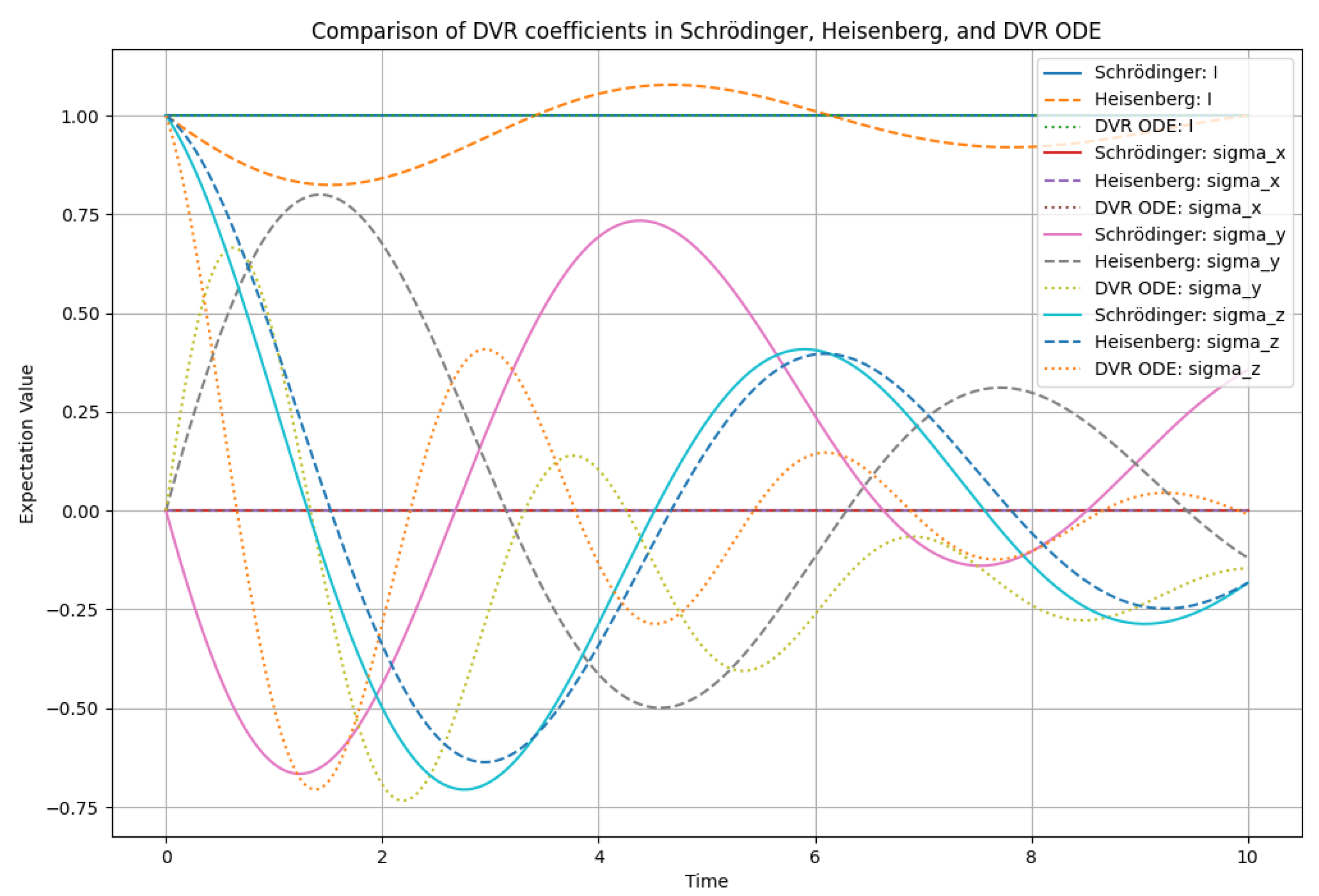
Figure 2.
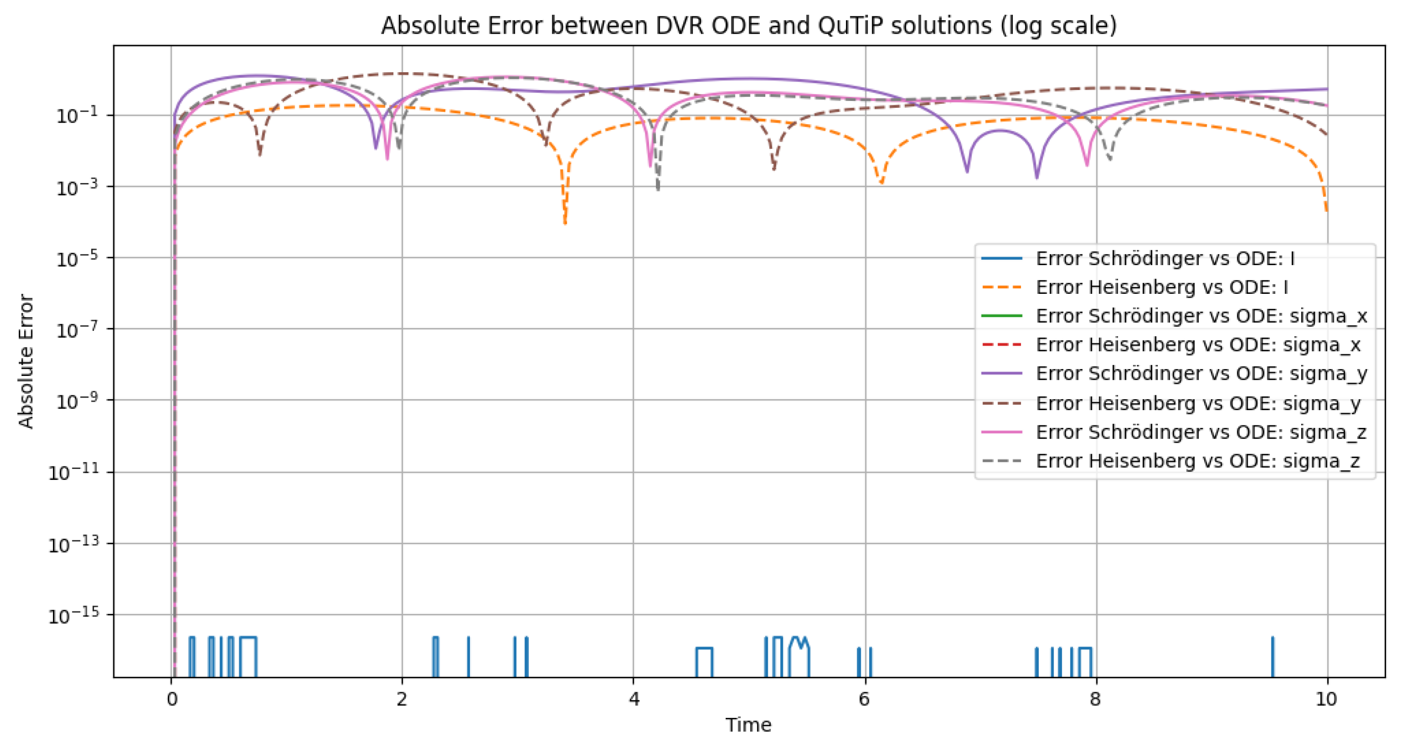
Absolute errors (log scale) comparing DVR ODE solutions to QuTiP Schrödinger and Heisenberg evolutions for all Pauli basis observables. Trace preservation is exact to machine precision (errors ), while Pauli observable errors remain bounded, typically below 0.1. This demonstrates the accuracy and stability of the DVR coefficient evolution approach in reproducing Lindblad dynamics across all observables.
Figure 2.
Absolute errors (log scale) comparing DVR ODE solutions to QuTiP Schrödinger and Heisenberg evolutions for all Pauli basis observables. Trace preservation is exact to machine precision (errors ), while Pauli observable errors remain bounded, typically below 0.1. This demonstrates the accuracy and stability of the DVR coefficient evolution approach in reproducing Lindblad dynamics across all observables.
This numerical validation provides strong empirical support for the theoretical claims of the theorem, particularly confirming that:
- The Lindblad master equation indeed induces a closed system of ODEs for the DVR coefficients (Point 3 of the Theorem).
- The evolution of DVR coefficients is equivalent to Heisenberg-picture expectation dynamics (Point 4 of the Theorem).
The ability to accurately track and predict observable moments through a direct ODE system in coefficient space, validated against both Schrödinger and Heisenberg pictures, underscores the practical utility and theoretical consistency of the DVR framework for analyzing and controlling open quantum systems.
5. Conclusion
The Observable Hierarchy Representation and Pathwise Evolution Theorem establishes Difference-Based Variational Reconstruction (DVR) as a robust and profoundly insightful framework for quantum dynamics and control. By expanding the quantum state in an orthonormal operator basis, DVR coefficients directly provide a complete coordinate system for the quantum observable hierarchy, encompassing all moments and correlations.
This formulation offers a powerful unification of core quantum mechanical formalisms:
- Heisenberg Picture: The evolution of DVR coefficients is shown to be precisely equivalent to the evolution of Heisenberg-picture expectation values, providing a direct computational pathway for operator dynamics, naturally extended to open systems via the Lindblad superoperator.
- Path Integral Formulation: The time trajectories of DVR coefficients define paths in observable-moment space. The associated real-valued action functional allows for a path integral formulation that is analogous to statistical-mechanical path integrals and the Feynman–Vernon influence functional for dissipative systems, offering a unique perspective on quantum dynamics in the presence of an environment.
The profound physical meaning of this DVR framework lies in its ability to directly represent and control quantum systems in the space of their observable moments, which are inherently measurable quantities. This unification streamlines the process of quantum control design, diagnostics, and the fundamental understanding of decoherence and entanglement. By collapsing complex integral inversions into direct, regularized linear algebra in coefficient space, DVR provides a computationally tractable yet theoretically rich approach to managing the complexities of scalable quantum technologies. This methodological contribution, demonstrated across both quantum and classical PDE control problems, offers a new paradigm for designing robust and interpretable control strategies in function and operator spaces. Relation to Prior Work. Our previously published [5] approach to DVR-based quantum control can be seen as a direct application of this general framework. There, we designed adaptive feedback controllers to minimize the same slope-matching functional in DVR coefficient space. By selecting and stabilizing dominant DVR modes, we demonstrated coherence preservation even under strong Lindblad noise. This prior work thus represents a special case of the present formalism, where the variational principle is used explicitly to design real-time control strategies.
References
- G. Lindblad, “On the Generators of Quantum Dynamical Semigroups,” Commun. Math. Phys. 48, 119–130 (1976).
- H.-P. Breuer and F. Petruccione, The Theory of Open Quantum Systems, Oxford University Press, 2002.
- R. P. Feynman and F. L. Vernon Jr., “The Theory of a General Quantum System Interacting with a Linear Dissipative System,” Annals of Physics 24, 118–173 (1963).
- J. R. Johansson, P. D. Nation, and F. Nori, “QuTiP 2: A Python framework for the dynamics of open quantum systems,” Comput. Phys. Commun. 184, 1234–1240 (2013).
- R. Acharyya, “Function-Space Quantum Control via Difference-Based Variational Reconstruction: A Scalable Framework for Coherence Preservation,” 2025.
Disclaimer/Publisher’s Note: The statements, opinions and data contained in all publications are solely those of the individual author(s) and contributor(s) and not of MDPI and/or the editor(s). MDPI and/or the editor(s) disclaim responsibility for any injury to people or property resulting from any ideas, methods, instructions or products referred to in the content. |
© 2025 by the authors. Licensee MDPI, Basel, Switzerland. This article is an open access article distributed under the terms and conditions of the Creative Commons Attribution (CC BY) license (http://creativecommons.org/licenses/by/4.0/).
Copyright: This open access article is published under a Creative Commons CC BY 4.0 license, which permit the free download, distribution, and reuse, provided that the author and preprint are cited in any reuse.


