
Submitted:
10 November 2025
Posted:
13 November 2025
You are already at the latest version
Abstract
Accurate estimation of the open-circuit voltage (OCV) as a function of state of charge (SOC) is fundamental for reliable battery management system (BMS) design in lithium-ion battery applications. However, at low temperatures, traditional low-rate OCV testing methods suffer from polarization-induced voltage drops that truncate the measured voltage range. This results in capacity underestimation and distorted OCV–SOC profiles, directly impacting SOC estimation accuracy. In this paper, we demonstrate how low-temperature conditions can severely distort the OCV-SOC models due to elevated polarization leading to premature voltage cutoffs. This paper presents a novel offsetting based correction method that extrapolates the charge/discharge curves beyond polarization-induced cutoff points to recover the full OCV span that otherwise would be lost at low temperatures. The approach is demonstrated using experimental low-rate OCV characterization data collected from Samsung EB575152 Li-ion cells from negative −25°C to 50°C. Results show that the proposed method significantly restores the usable OCV-SOC profile without requiring any modifications to the standard low-rate test protocol. By preserving complete voltage curves across a wide temperature range, this technique significantly improves the SOC estimation accuracy for battery management system.
Keywords:
battery modeling
; battery management systems
; lithium-ion batteries
; open-circuit voltage model
; low-temperature performance
; state-of-charge estimation
I. Introduction
Lithium-ion (Li-ion) batteries have become the cornerstone of energy storage for electric vehicles (EVs) and other high-performance applications due to their superior energy density, long cycle life, efficiency, reliability, and affordability [2,3,4]. Ensuring safe and efficient operation of these batteries requires continuous monitoring by a battery management system (BMS), with accurate state-of-charge (SOC) estimation being especially critical because SOC errors can compound into reduced lifespan or safety risks [5,6]. Among various SOC indicators, the open-circuit voltage (OCV) measured at (quasi-)equilibrium is widely used because OCV exhibits a near-monotonic relationship with SOC and the OCV–SOC map is relatively stable against ageing and temperature variations [2,7]. At the same time, TTE studies highlight chemistry- and condition-specific complications that can bias OCV-based estimation, including plateau regions and temperature-dependent deviations that introduce OCV–SOC curve errors (e.g., in LiFePO4 cells) [8], as well as ageing-induced shifts that must be anticipated over long service lifetimes, where physics-guided machine learning has shown promise in forecasting degradation trajectories and knee points [9]. Consequently, establishing an accurate, temperature- and ageing-aware OCV–SOC characterization remains fundamental for both offline calibration and real-time SOC estimation in modern EV BMS.
Over the years, numerous approaches have been developed to model the nonlinear OCV-SOC relationship for use in BMS algorithms. Among these, the Galvanostatic Intermittent Titration Technique (GITT) and the low-rate cycling method are important ones [10]. In the GITT approach, individual OCV-SOC points are measured intermittently and recorded in a way that the resulting OCV-SOC data spans the entire SOC range. Here, the SOC is changed by applying a constant current [11]. Existing standards stipulate discharging the cell in steps and applying a 10-second charge/discharge pulse at each step to estimate other battery parameters such as the resistance and RC components. The rest of 1 hour is standardized for allowing the battery to achieve cell equilibrium potential. Just before the next discharge step, the OCV is measured. In the low-rate cycling approach (see [12,13] for a review), a battery is discharged and then charged using the same low C-Rate while continuously collecting the voltage and current data. Owing to the low current rate, the low-rate cycling method is also called the Coulomb titration (CT) technique. The advantage of the low-rate OCV modeling approach over the GITT method is that the former enables high resolution OCV-SOC data in a relatively short time.
The focus of the present paper is on the low-rate OCV testing approach. It is shown in this paper that, this conventional method suffers from notable shortcomings when applied at low temperatures. Increased internal resistance at subzero conditions causes the battery voltage to prematurely reach cutoff thresholds, leading to early termination of charging and discharging steps. Consequently, the measured voltage profiles are truncated, resulting in underestimated usable capacity and a compressed SOC window. This ultimately distorts the OCV-SOC curve, which can bias SOC estimation and degrade BMS performance. While several studies have proposed strategies such as redefining SOC limits or adjusting for capacity loss [7], the specific issue of voltage truncation caused by polarization effects remains inadequately addressed. In practice, truly capturing the entire OCV-SOC curve at sub-freezing conditions would require either extremely long relaxation periods at many intermediate SOC points (as part of the GITT procedure) or accepting a truncated curve and then applying elaborate post hoc corrections. A clear gap remains for a simple yet effective procedure to retain the complete OCV-SOC profile under cold-temperature testing without resorting to impractical protocols.
In this paper, we introduce a novel offsetting-based correction method to address the low-temperature OCV truncation problem. The key idea is to extrapolate the OCV curve beyond the points where the standard test had to stop, by applying an appropriate voltage offset to the end-of-charge and end-of-discharge portions of the measured curve. In essence, the method projects what the terminal voltage would have been at 100% SOC (above the upper cutoff) and at 0% SOC (below the lower cutoff) if the cell were not limited by polarization. This can be implemented in a straightforward manner: for example, by linearly extrapolating the tail end of the discharge voltage vs. time curve to estimate the missing segment beyond the lower cutoff. While overcharging or overdischarging the battery is not feasible in live systems due to risks like thermal runaway [14,15], degradation [16], and uncertain safe margins, such extrapolation can be performed safely in an offline modeling context. Our method accounts for the voltage drop induced by internal resistance and effectively restores the full OCV range (e.g., 3.0 V to 4.2 V) without modifying the standard testing procedure.
The proposed offset methods can be informed by simple models (e.g. using the internal resistance to estimate the IR drop) to improve accuracy, but importantly, no modifications to the standard test procedure are required, i.e., the battery is not actually over-discharged or over-charged; all adjustments are done in post-processing. By applying these linear or model-based offsets at the SOC boundaries, the full OCV span (from true minimum voltage, , at 0% SOC to the true maximum voltage at 100% SOC) is reconstructed, effectively recovering the OCV range lost due to low-temperature polarization. The effectiveness of the proposed offsetting method is demonstrated using experimental data from lithium-ion cells (Samsung EB575152) tested across a broad temperature range from -25 to 50.
Under conventional low-rate testing, it is observed that the colder the temperature, the more severely the voltage curve is truncated and the actual capacity underreported — confirming the known limitation of the standard protocol. By contrast, applying the proposed voltage offsets at the cutoff points yields OCV-SOC curves that closely match the full 0–100% SOC behavior expected at each temperature. The corrected curves show that the intended voltage span is restored at all temperatures. To quantify the improvements, we introduce three performance metrics: (i) the voltage offset at SOC boundaries, which directly measures the recovered voltage gap at low/high SOC; (ii) the cell-to-cell (C2C) variation in OCV, indicating whether the correction increases measurement consistency across different cells; and (iii) the temperature-induced OCV variation, evaluating how much the OCV curve shifts with temperature before and after applying the offset. These metrics provide a rigorous basis to assess the accuracy and robustness of the corrected OCV profiles. The results show that the offsetting approach significantly reduces the apparent capacity loss at low temperatures and narrows the disparity between OCV curves at different temperatures, thereby enhancing the fidelity of OCV-SOC modeling for BMS applications.
The remainder of this paper is organized as follows. Section II describes the OCV measurement procedure and analyzes the effect of temperature on low-rate OCV testing, highlighting the problem of truncated curves at cold temperatures. Section III details the proposed offsetting methodology, including the extrapolation technique and implementation considerations. Section IV presents a theoretical analysis and justification of the proposed method. Section V presents and discusses the experimental results and Section VI concludes the paper with a summary of contributions and suggestions for future work.
II. Problem Description
Figure 1a shows the voltage of the battery during the low-rate OCV test, C/30 discharge followed by C/30 charge, at different temperatures. In low-rate OCV modeling, the battery is considered full when the voltage is at and it is considered empty when the voltage is at Using this fact, the SOC is scaled between 0 and 1 separately during discharging and charging. Figure 1b shows the measured voltage of the battery against the SOC for sixteen different temperatures.
The OCV-SOC curves obtained through the low-rate OCV modeling approach summarized in Section I is shown in Figure 3. Here, a significant variance in the OCV values can be noticed. Before investigating the effect of temperature on the OCV-SOC curve, the focus will be placed on removing errors due to the low-rate OCV modeling approach.
Figure 2.
Measure Voltage against SOC for different temperatures.
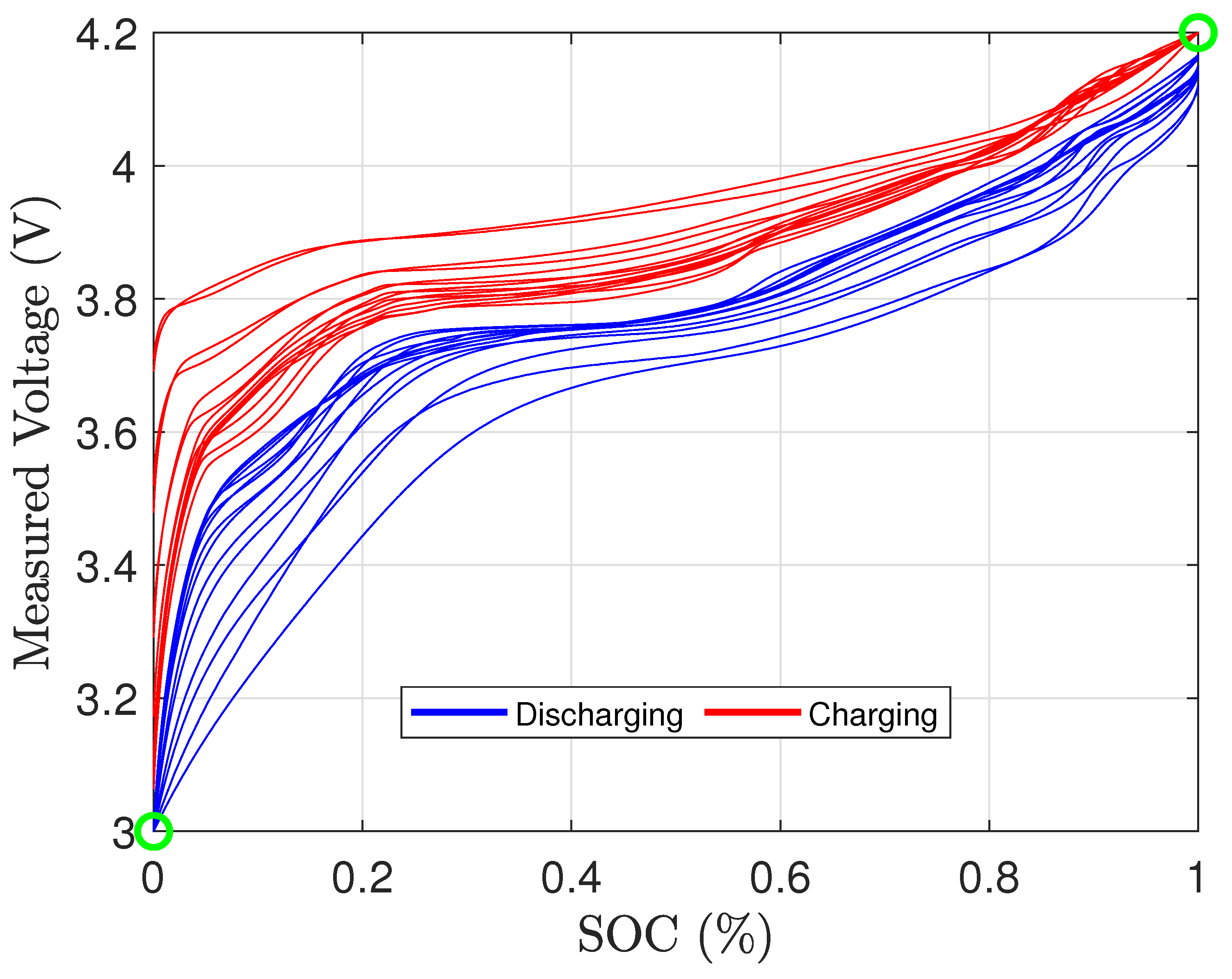
Figure 3.
OCV-SOC curves obtained through traditional low-rate OCV modeling approach.
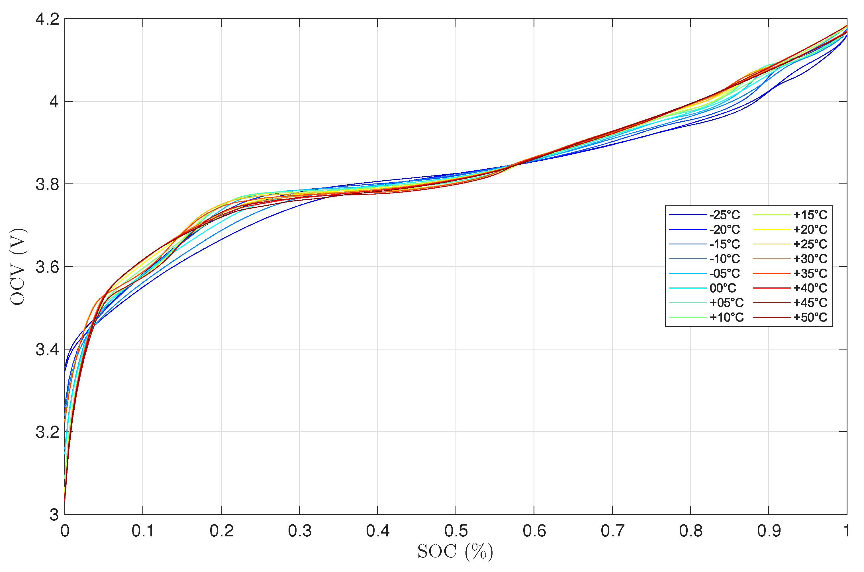
Figure 4a shows the total resistance of the battery. It can be noticed that the resistance significantly increases at cold temperatures. Due to the increase in resistance, the charging/discharging activity is prematurely terminated; this can be clearly seen in Figure 1. Due to premature termination of charging/discharging, the battery capacity is underestimated; this in turn affects the computed SOC that was always scaled between 0 and 1 in the low-rate OCV modeling approach [12]. It is possible that the computed OCV-SOC curve is affected as a result. Section III details an approach to ease the effect of the resistance in the computed OCV-SOC curve of the battery.
Figure 5.
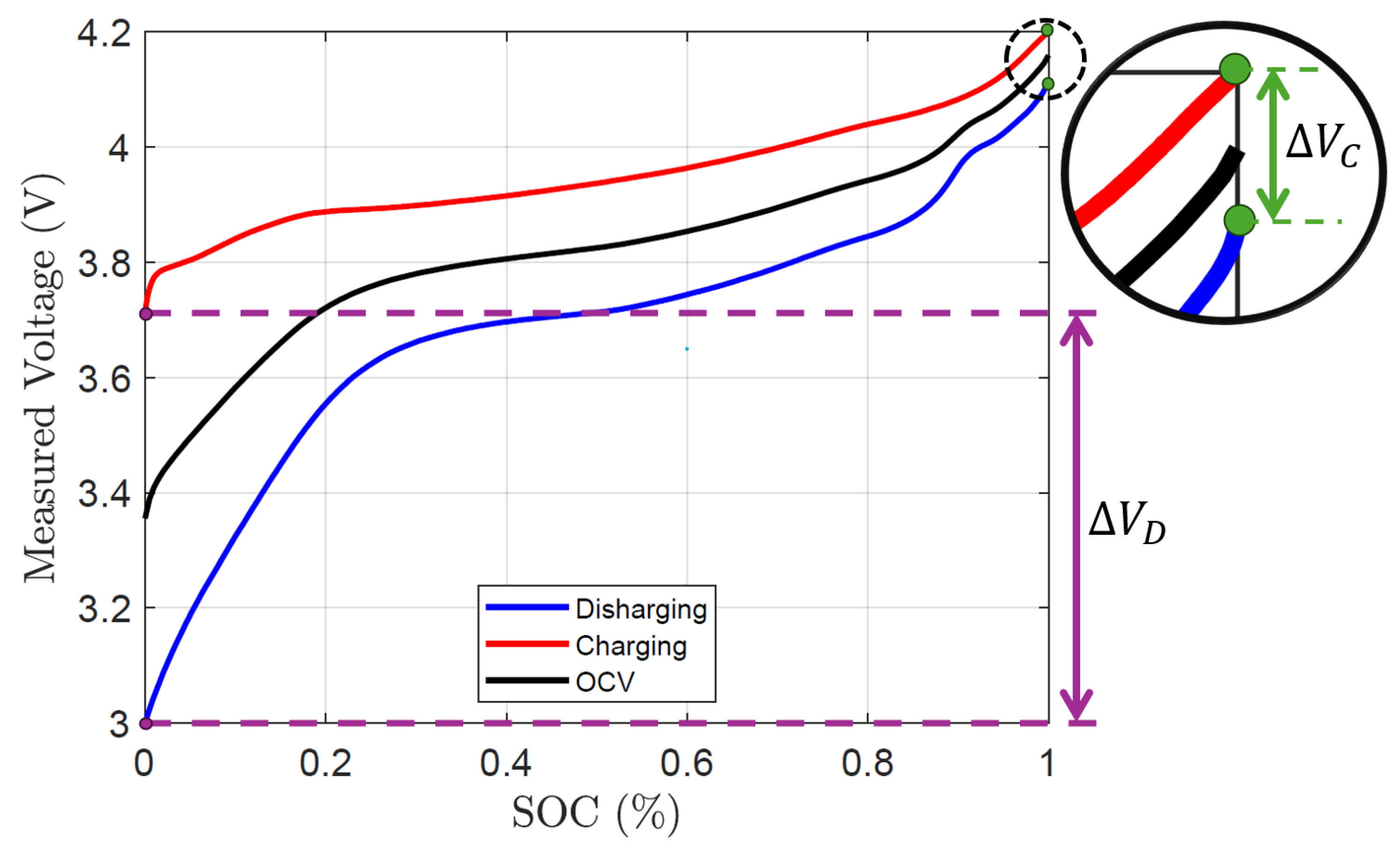
OCV-SOC curve of -25 ∘C obtained through averaging of discharge and charge curve.
III. Proposed Offsetting Approach
Figure 1b shows the measured terminal voltage at each temperature during both discharging and charging with respect to the SOC. Figure 2 is another representation of Figure 1b, where the terminal voltages at various temperatures are categorized into charging (indicated in red) and discharging (indicated in blue). It is noticed that for all the temperatures tested, the terminal voltage is lower than the OCV when discharging and higher when charging. Thus, the two terminal voltages for each respective temperature are averaged and is considered as the OCV for each SOC point. This is shown in Figure 3. From the resulting OCV-SOC curves, none of the temperatures tested ever reached the desired minimum OCV () when the battery was considered empty (s = 0) and maximum OCV () when the battery is considered full (s = 1). This is a direct consequence of the collected data stopping every test when the terminal voltages reach or when discharging and charging, respectively.
Figure 5 shows the most extreme case of this problem where the test temperature was -25 ∘C. At s = 0, the discharge and charge terminal voltages were 3V and 3.71V, respectively. Thus, the OCV value will be 3.3515V when they are averaged. Similarly, at s = 1, the resulting OCV value through averaging will be 4.1595V. This process is performed on the entire domain of the SOC, , and the resulting OCV-SOC curve is represented by the black line. It is clearly seen that the resulting curve does not have the desired and when averaged. It is also noticed that when we inspect Figure 3 again, when the temperature decreases, the OCV value when s = 0 and s = 1 is seen to be deviating further away from our desired and , respectively. This results in the OCV range becoming more skewed as the temperature decreases. In the remainder of this section, an approach is presented to fix this problem by extending the charge and discharge curve for each temperature by their respective voltage drop. With this approach, all of the OCV-SOC curves will span the same intended OCV range.
From Figure 5, the distance between the charge and discharge curve is calculated as:
where, , is the charge terminal voltage, , is the discharge terminal voltage, , is the voltage difference when the battery is empty, and , is the voltage difference when the battery is full.
These distances, and , are now used to extend the raw discharge and charge curves to offset the voltage differences. In Figure 6, it is seen that the discharge curve is extended further down by , represented by the magenta line and the charge curve is extended further up by represented by the green line. When , will remain the same and the new will be the end value of the extended magenta line. Similarly, when , will remain the same and the new will be the end value of the extended green line. Figure 7 shows how this approach achieves the desired and by extending the curves and accounting for the voltage drop. When the battery is empty, the charge and new discharge terminal voltage was 3.71V and 2.31V, respectively. Thus, the OCV value computed by averaging will be 3V. Similarly, when the battery is full, the resulting OCV value will be 4.2V when averaged.
For extending the charge and discharge curve, a linear extrapolation is used to find the extended data for this approach. In Figure 6, the final five data points (time and their corresponding terminal voltages) at the end of the raw discharge curve and the first five data points of the beginning of the raw charge curve are taken. Separately, the points from the discharge curve and the charge curve are then each linearly fitted using the least squares method to find the lines that best fit those selected points. The two slopes are then averaged together and the resulting slope, represented by the magenta line is used to extend the data by the offset voltage difference, . It is important to note that since the slope of the charge curve will be positive, the negative value will be taken to correctly average the two. Now, 650 data points are taken from the end of the charge curve and the slope, represented by the green line is found through the least squares method. With this, the slope is extended upward by . With these offsets, the curves are extrapolated until they reach the point where the voltage will offset the voltage differences. Figure 7 shows the corrected offset of the charge and discharge curve where now the OCV curve has the desired voltage range.
This offsetting approach is repeated on the remaining temperatures and the OCV-SOC curves for all of them are shown in Figure 8. In Figure 3, the and are all different for each temperature as a result of the varying voltage drop. This problem was fixed in the OCV-SOC curve obtained from the proposed offsetting approach.
It is important to note that a previous offsetting approach was presented in a conference version based on this method. These two proposed approaches were called Offsetting Approach I (OA-I) and Offsetting Approach II (OA-II). The difference between these two approaches is shown in Figure 9 where OA-II is considered to be our Proposed Offsetting Approach in this section.
IV. Theoretical Simulation Analysis
To further show the effect of the Proposed Offsetting Approach on the OCV-SOC curve, a theoretical simulation is conducted using a battery simulator to simulate the low-rate OCV test. The voltage and current measurements are generated using the R-int electrical equivalent circuit model (EECM). The R-int EECM is shown in Figure 10, where the terminal voltage can be written as:
where is the current measurement through the battery, is the OCV effect and is the resistance.
When considering measurement noise, the measured voltage and current are written as:
where the voltage and current measurement errors and are assumed to be zero-mean with standard deviations and , respectively.
Figure 11 shows the battery simulator representation showing how , and the SOC are generated as explained in the following:
- 1.
- Battery Capacity and SOC: To simulate the battery to be as close to that of the real test with Samsung EB575152, the same rated capacity is used by the simulator. Thus, the assumed true battery capacity is set to 1.5 Ah for this simulation. To replicate a C/30 discharge and charge, the current is found to be . The SOC is recursively computed using the Coulomb counting approach:where is the time difference between two measurements in seconds, is the current measurement through the battery in Amperes, and Q is the true battery capacity in Ampere hour (Ah).
- 2.
- OCV Model: Using the combined+3 model [12], the OCV, , of the battery is computed by applying the following parameters:
- 3.
- EECM Model Parameters: To simulate varying temperatures, the internal resistances will start from and sequentially decrease by until is reached. Since resistance increases as temperature decreases, Table 1 shows the temperature-dependent resistance used in this simulation.
- 4.
- Noise Statistics: The voltage and current measurement noise are assumed to be and , respectively.
Now, given a , the battery is simulated where it is assumed full at the start, . The battery is then discharged using a constant current of until it reaches . Next, the battery is charged using a constant current of until it reaches .
Figure 12 shows the terminal voltage for the varying internal resistances. Similar to the experimental data shown in Figure 1a, the simulation tests in Figure 12 are all stopped at when discharging and when charging, which underestimates the battery capacity, and consequently, affects the OCV-SOC curve.
Figure 13 shows the measured voltage of battery against the SOC when assuming the same capacity for every temperature test. It is noticed as a result of the low-rate OCV test procedure, the test is stopped prematurely as the resistance increases. For example in the figure, when the resistance is set to 3 , which represents a very low temperature, the terminal voltage when charging is seen to only reach about an SOC value of 0.85 since the test needs to be stopped when is reached. Now, since this traditional approach always scales each curve from 0 to 1 [12], this results in the charging and discharging curves to become truncated. This is seen in Figure 14 where the skewing due to the test procedure becomes evident. Figure 15 shows the resulting OCV-SOC curves at all resistances or the equivalent temperatures in Table 1. From this, it is seen that the OCV-SOC curve is affected by the unaccounted for voltage drops, resulting in variation at the high and low end of the SOC. Figure 16a,b show an enlarged image of the low and high end SOC, respectively.
Figure 17 shows the Proposed Offsetting Approach presented in Section III where instead of limiting all tests to the same and , each test is offset by its respective voltage drop. Figure 18 shows the terminal voltage of the battery when charging and discharging where it is noticed how now instead of all the temperatures being truncated, the voltages curves for each resistance will now correctly span the whole SOC range due to the Proposed Offsetting Approach extrapolating past the voltage cutoffs and accounting for the voltage drop. Now, the OCV-SOC curve is shown in Figure 19 where all the curves are found to be nearly identical with very little variance. This demonstrates that in theory, using the Proposed Offsetting Approach, should correctly fix the voltage drop issue allowing for similar OCV-SOC curves regardless of the internal resistance or temperature variations. However, this is clearly not what is happening when the approaches are applied to the real test data especially at lower SOC and very low temperatures. Thus, it is evident that simply representing the temperature by only changing the internal resistance is not entirely accurate.
V. Experimental Results
To assess the effectiveness of the Proposed Offsetting Approach mentioned in Section III against the traditional low-rate OCV approach, three metrics are introduced and explained in the remainder of this section.
The OCV curves of all tested temperatures and batteries are summarized by Table 2. Thus, the OCV curve can be represented by where q, is a particular battery, r, is a particular test temperature and , is the number of SOC points. For this paper, the total number of temperatures tested are, , the total number of cells are, , and the number of SOC points, were selected.
A. Performance Evaluation Metrics
1. Low-End and High-End Offset
For the low-end, , the for all temperatures is expected to be . Thus, for a particular temperature, r, the mean low-end offset, is calculated as:
where j in this case will be representing SOC = 0 and is the number of batteries tested.
Similarly, for the high-end, , the for all temperatures is expected to be . Thus, for a particular temperature, r, the mean high-end offset, is calculated as:
where j in this case will be representing SOC = 1 and is the number of batteries tested.
Thus, the computed and for each temperature is represented by Table 3.
2. Cell-to-Cell Variation
For a particular temperature, r, the OCV data is chosen from Table 2 for the number of battery cells, . For this, two cell-to-cell variation metrics are computed. These are the mean, and standard deviation, which are computed as:
where denotes the binomial coefficient of all possible number of combinations of pairs for cells (See Remark 1). So, the OCV data difference between every possible combination of cells is taken and then averaged. It is important to note that the calculated mean in (9) and standard deviation in () are vectors of length j which spans the SOC range.
Remark 1.
Let us consider the case where four battery cells ( = 4) are tested to evaluate cell-to-cell (C2C) variation. In this case, the total number of combinations of cells is six possible pairings ( = 6) that are unique. We can have cells (1,2), (1,3), (1,4), (2,3), (2,4), and (3,4). Thus, in equations 9 and 10, the C2C variations are computed by evaluating the difference in OCV values at each SOC point between every possible pair. This ensures that the variation is not biased toward any single cell and will reflect the overall spread in behavior across every tested battery instead. Thus, any cell can be chosen as a reference, as all variation of each cell is taken into account.
Thus, the computed and for each temperature is be represented by Table 4.
3. Temperature Variation
Again, the OCV data is chosen from Table 2. For a particular temperature, r and all battery cells, , the two temperature error metrics, mean, and standard deviation, are computed as:
where the test number is chosen to be the reference OCV in which the other OCV curves are to be compared against. It is important to note that the calculated mean in (11) and standard deviation in (10) are vectors of length j which spans the SOC-Grid.
Thus, the computed and for each temperature is be represented by Table 5.
B. Evaluation Results
In this section, the computation of three metrics: low-end and high-end offset, cell-to-cell variation and temperature variation explained in Section A.
1. Low-End and High-End Offset
For the traditional approach, the mean low-end offset, is calculated using equation (7). The offsets are tabulated and shown in Table 6. It is seen how the of each temperature is affected due to these offsets especially at very low temperatures such as C where the offset is off the expected of .
The mean high-end offset, is calculated using equation (8). The offsets are tabulated and shown in Table 7. Unlike for the low-end offset, all temperatures offset are not too far off of the expected of . The highest offset is around for the lowest temperature, C.
It is important to note that for the Proposed Offsetting Approach, the low-end and high-end offset will be zero for all temperatures since the whole goal of the Offsetting Approach is to remove the effects of low and high-end offset.
2. Cell-to-Cell Variation
From computing the mean, in (9) and standard deviation, in (10), the cell-to-cell (C2C) variation at every temperature are found for all three approaches and compared. The C2C variation will span the entire SOC range between SOC = 0 and SOC = 1. Figure 20a,b show the C2C variation at every temperature for the Traditional Approach and the Proposed Offsetting Approach, respectively. The filled in region for each temperature represents the window of uncertainty where the OCV value can fluctuate around and is between . Thus, the uncertainty width of a given j SOC point is . With this definition, the max value of for all temperatures spanning the whole SOC is around . Upon inspection, the uncertainty widths did show some observable patterns for the differences between temperatures. For both approaches, the C2C variation tend to increase at the lower SOC region with the largest being around an uncertainty width of around at SOC = 0.1. Another observation is that both approaches have peak C2C uncertainty width at the same SOC at the highest temperature range (C).
3. Temperature Variation
For the reference temperature, , the room temperature, 25 ∘C was chosen as the standard OCV-SOC curve. For the three approaches, the uncertainties in OCV values are calculated for all 16 temperatures for the entire span of the SOC range between SOC = 0 and SOC = 1. Figure 21a–c show the temperature variations of all three approaches for -25 ∘C, 10 ∘C and 50 ∘C, respectively. The defined window of uncertainty in which the OCV value can fluctuate around is between .
While comparing approaches at a very low temperature of C, it can be noticed how large of an uncertainty the traditional approach yields at with an uncertainty width, of around . For the Proposed Offsetting Approach, the uncertainty at will be almost zero as all OCV-SOC curves are made to have the same . However, it can seen that an increase in uncertainty between the low SOC range of 0.05 and 0.3 has happened as a result with peak of around . At higher SOC, the offsetting approach shows much lower uncertainty as compared to the traditional approach. Most notably, it is seen how even at the lowest temperature, the uncertainty window to have decreases compared to the traditional approach
For 10 ∘C, it can be seen that there is not much uncertainty with all approaches with the peak uncertainty width, being around of all approaches at an . This suggests that as the temperature increases to around the room temperature of 25 ∘C, the OCV-SOC curves become much more similar. It is also noticed that even for higher temperatures, the Proposed Offsetting Approach still results in lower uncertainty at higher SOC compared to the traditional approach.
Finally, for the highest temperature of 50 ∘C, the peak value of are larger than 10 ∘C, with the traditional having and Proposed Offsetting Approach having .
Figure 22a,b shows the uncertainties of the traditional approach and Proposed Offsetting Approach for all temperatures using the computed mean and standard deviation in (11) and (), respectively. Here we can now see the variations at all temperatures when compared to 25 ∘C. Comparing these two approaches, the offsetting approach shows a very large at lower SOC for low temperatures. This is in exchange for the large uncertainty window when SOC = 0 for the traditional approach. It is also noticed how at the high SOC region, the uncertainty window for the Proposed Offsetting Approach noticeably decreases when compared to the traditional approach.
VI. Conclusions
This study identified a critical limitation in the standard low-rate OCV testing method for lithium-ion batteries—its tendency to truncate voltage curves at low temperatures due to elevated polarization. This premature cutoff results in underestimated capacities and skewed OCV–SOC profiles, narrowing the effective SOC window and reducing the accuracy of BMS algorithms.
To mitigate this, we introduced a straightforward offsetting-based correction method. By extrapolating the voltage curves beyond their cutoff limits—based on the observed voltage gap at SOC boundaries—we recovered the full voltage span that would otherwise be lost to temperature-induced polarization. This approach avoids the safety and degradation risks of actual overcharging or overdischarging and is applicable during offline characterization.
Experimental validation was conducted using a Samsung EB575152 cell across a wide temperature range (C to C), supported by theoretical simulations using an internal resistance (R-int) model. Results showed that the proposed correction improves the voltage range consistency in the mid-to-high SOC region (SOC ≥ 0.4) and partially recovers lost capacity, particularly in cold-temperature tests. However, the lower SOC region (SOC < 0.4) still exhibits significant variability, suggesting that polarization and capacity loss at low temperatures are not solely governed by internal resistance.
Further, we evaluated both the traditional and proposed methods using three performance metrics: low/high-end offset, C2C variation, and temperature variation. These metrics confirmed that while the offsetting method effectively recovers OCV range and improves consistency in the upper SOC region, it introduces uncertainty in the lower SOC region, especially at low temperatures. The comparative analysis also revealed that cell-to-cell variation remains largely unaffected by the correction, indicating that inherent cell differences are not significantly altered.
In summary, the proposed correction method is a practical and low-risk enhancement to standard OCV testing. It restores lost capacity due to temperature effects, preserves the full usable OCV range, and improves SOC estimation accuracy without requiring additional tests or protocol changes. However, residual errors at low SOC and low temperature suggest that further modeling of non-ohmic behavior is needed for more accurate temperature-aware BMS design.
References
- J. Nguyen, P. Pillai, S. Sunil, and B. Balasingam, “An offsetting-based correction to improve the accuracy of low-rate ocv curves for lithium-ion batteries,” in IEEE International Symposium on Industrial Electronics. 2025. [CrossRef]
- F. Zheng, Y. Xing, J. Jiang, B. Sun, J. Kim, and M. Pecht, “Influence of different open circuit voltage tests on state of charge online estimation for lithium-ion batteries,” Applied Energy, vol. 183, pp. 513–525, 2016.
- L. H. Saw, Y. Ye, and A. A. Tay, “Integration issues of lithium-ion battery into electric vehicles battery pack,” Journal of Cleaner Production, vol. 113, pp. 1032–1045, 2016.
- P. H. Camargos, P. H. J. Santos, et al., “Perspectives on li-ion battery categories for electric vehicle applications: A review of state of the art,” International Journal of Energy Research, vol. 46, no. 12, pp. 17050–17074, 2022.
- C. Pan, Z. Peng, S. Yang, G. Wen, and T. Huang, “Battery state of charge estimation with event-triggered parameter identification,” IEEE Transactions on Transportation Electrification, vol. 10, no. 4, pp. 10401–10409, 2024.
- M. S. ElMenshawy, A. M. Massoud, and P. Guglielmi, “State-of-charge estimation using triple forgetting factor adaptive extended kalman filter for battery energy storage systems in electric bus applications,” IEEE Transactions on Transportation Electrification, vol. 11, no. 2, pp. 6664–6674, 2025.
- L. Ju, P. Long, G. Geng, and Q. Jiang, “Open circuit voltage - state of charge curve calibration by redefining max–min bounds for lithium-ion batteries,” Journal of Energy Storage, vol. 79, p. 110224, 2024.
- D. Paizulamu, L. Cheng, H. Xu, Y. Zhuang, N. Qi, and S. Ci, “LiFePO4 battery soc estimation under ocv–soc curve error based on adaptive multi-model kalman filter,” IEEE Transactions on Transportation Electrification, vol. 11, no. 4, pp. 8833–8846, 2025.
- X. Jia, C. Zhang, Y. Li, C. Zou, L. Y. Wang, and X. Cai, “Knee-point-conscious battery aging trajectory prediction based on physics-guided machine learning,” IEEE Transactions on Transportation Electrification, vol. 10, no. 1, pp. 1056–1069, 2024.
- A. Barai, K. Uddin, M. Dubarry, L. Somerville, A. McGordon, P. Jennings, and I. Bloom, “A comparison of methodologies for the non-invasive characterisation of commercial li-ion cells,” Progress in Energy and Combustion Science, vol. 72, pp. 1–31, 2019.
- J. P. Christophersen, “Battery test manual for electric vehicles, revision 3,” tech. rep., Idaho National Lab.(INL), Idaho Falls, ID (United States), 2015.
- P. Pillai, S. Sundaresan, P. Kumar, K. R. Pattipati, and B. Balasingam, “Open-circuit voltage models for battery management systems: A review,” Energies, vol. 15, no. 18, p. 6803, 2022.
- B. Balasingam, Robust Battery Management Systems With Matlab. Artech House, 2023.
- Y. Chen, Y. Kang, Y. Zhao, L. Wang, J. Liu, Y. Li, Z. Liang, X. He, X. Li, N. Tavajohi, and B. Li, “A review of lithium-ion battery safety concerns: The issues, strategies, and testing standards,” Journal of Energy Chemistry, vol. 59, pp. 83–99, 2021.
- J. D. Gotz, M. A. S. Teixeira, F. C. Corrêa, E. R. Viana, A. A. Badin, and M. Borsato, “The influence of overcharging and over-discharging on the capacity degradation of lithium-ion batteries,” in 2024 IEEE Vehicle Power and Propulsion Conference (VPPC), pp. 1–6, 2024.
- H. Maleki and J. N. Howard, “Effects of overdischarge on performance and thermal stability of a li-ion cell,” Journal of Power Sources, vol. 160, no. 2, pp. 1395–1402, 2006. Special issue including selected papers presented at the International Workshop on Molten Carbonate Fuel Cells and Related Science and Technology 2005 together with regular papers.
Figure 1.
Measured voltage during low-rate OCV test.
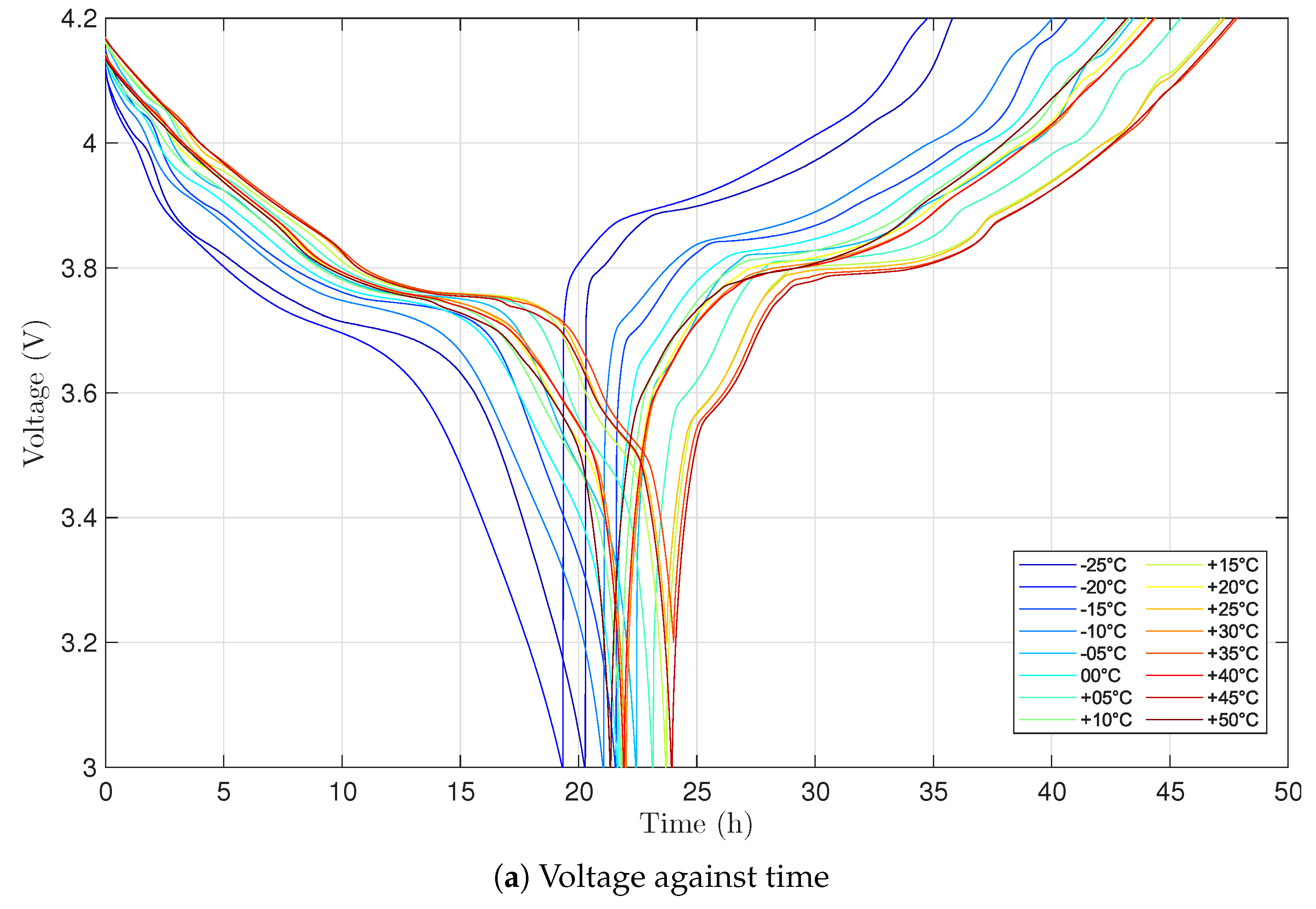
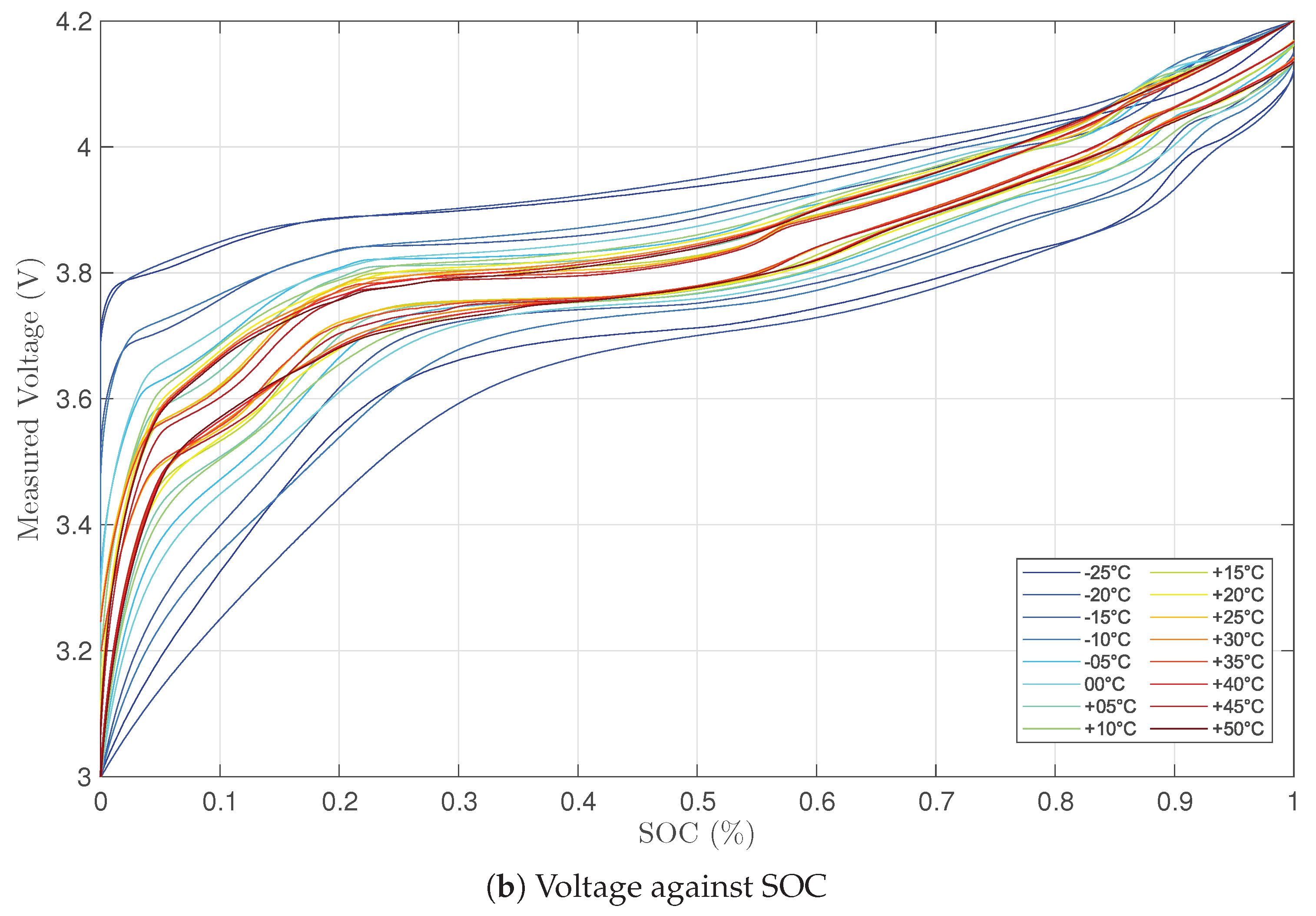
Figure 4.
Computed resistance and capacity of the battery.
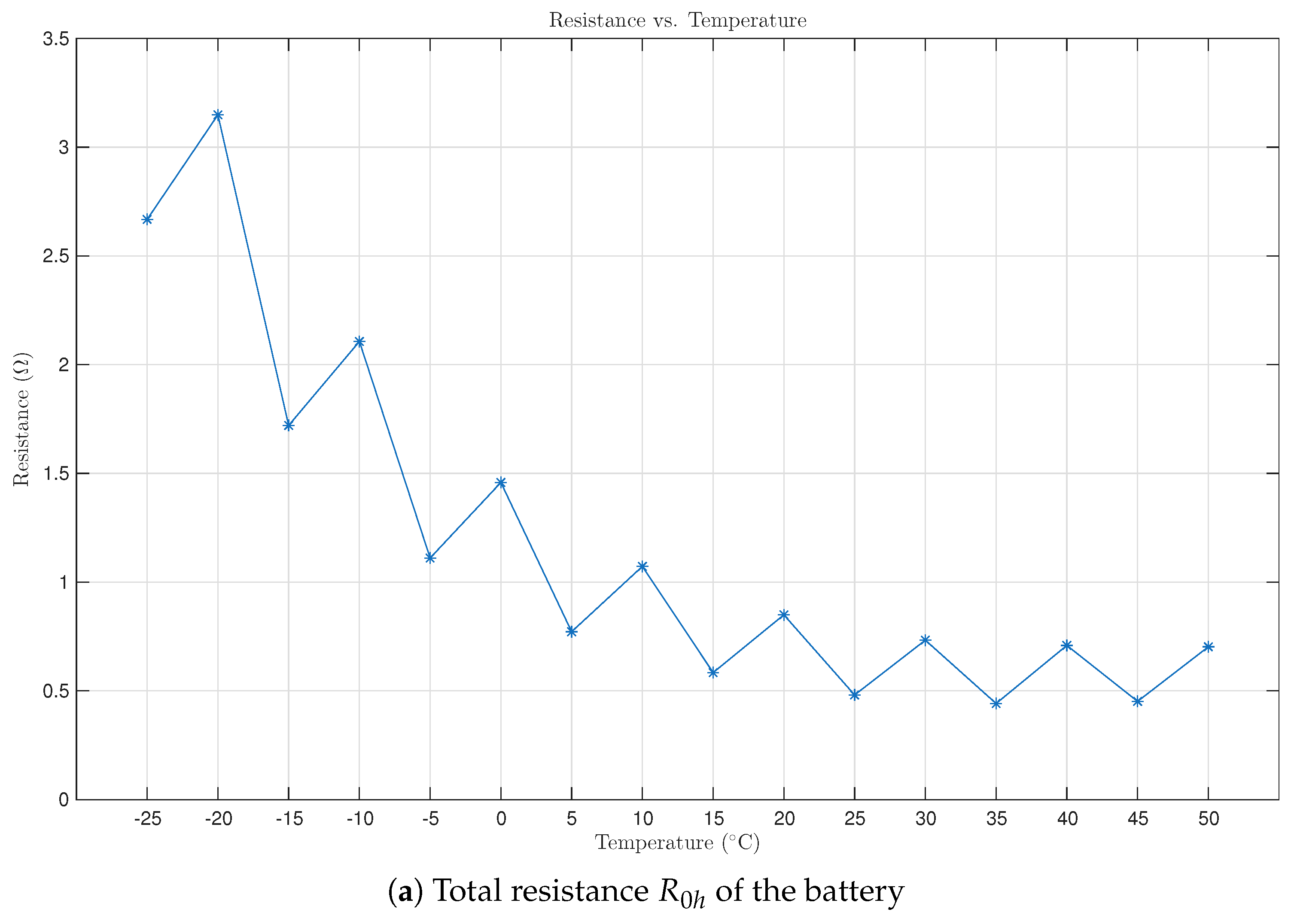
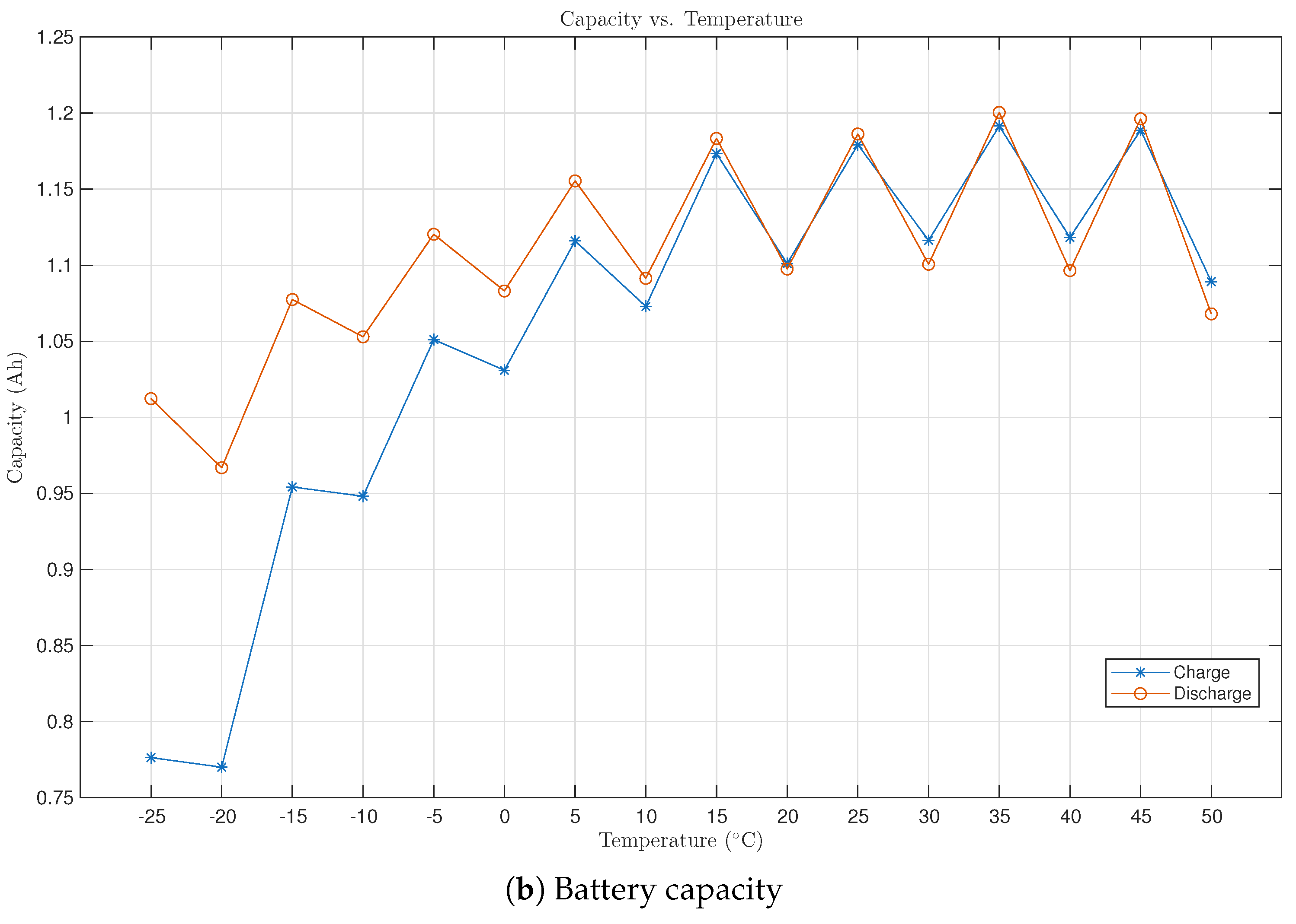
Figure 6.
Proposed Offsetting Approach for temperature: -25 ∘C
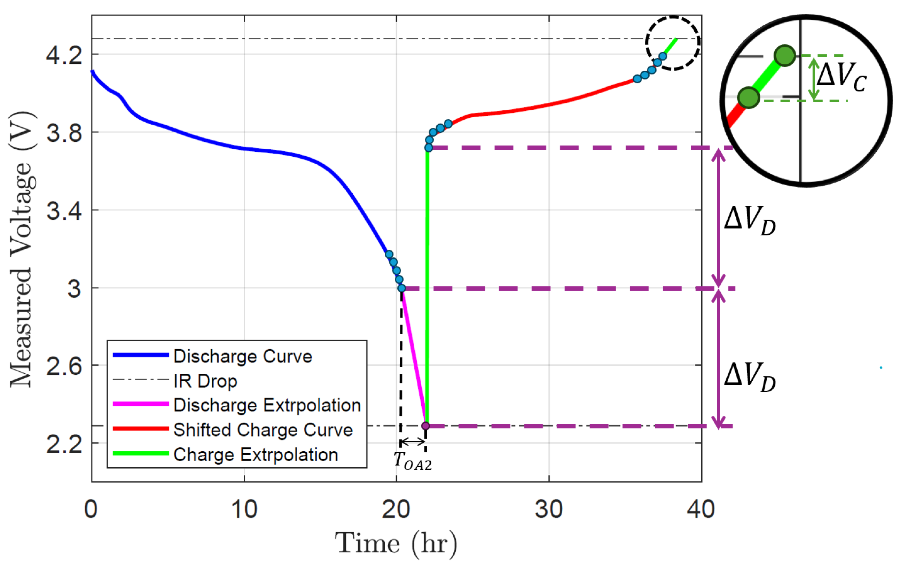
Figure 7.
Extrapolated Voltage against SOC - Proposed Offsetting Approach.
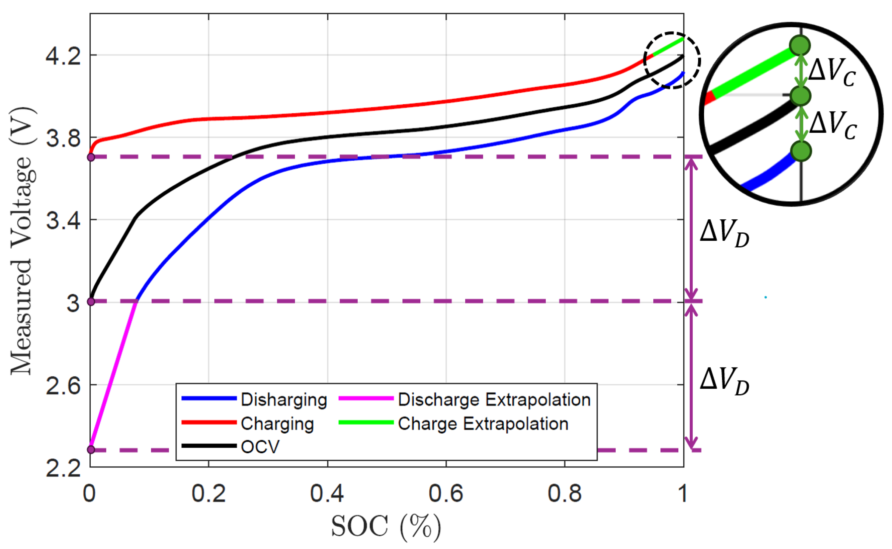
Figure 8.
Proposed Offsetting Approach - OCV-SOC Curve.
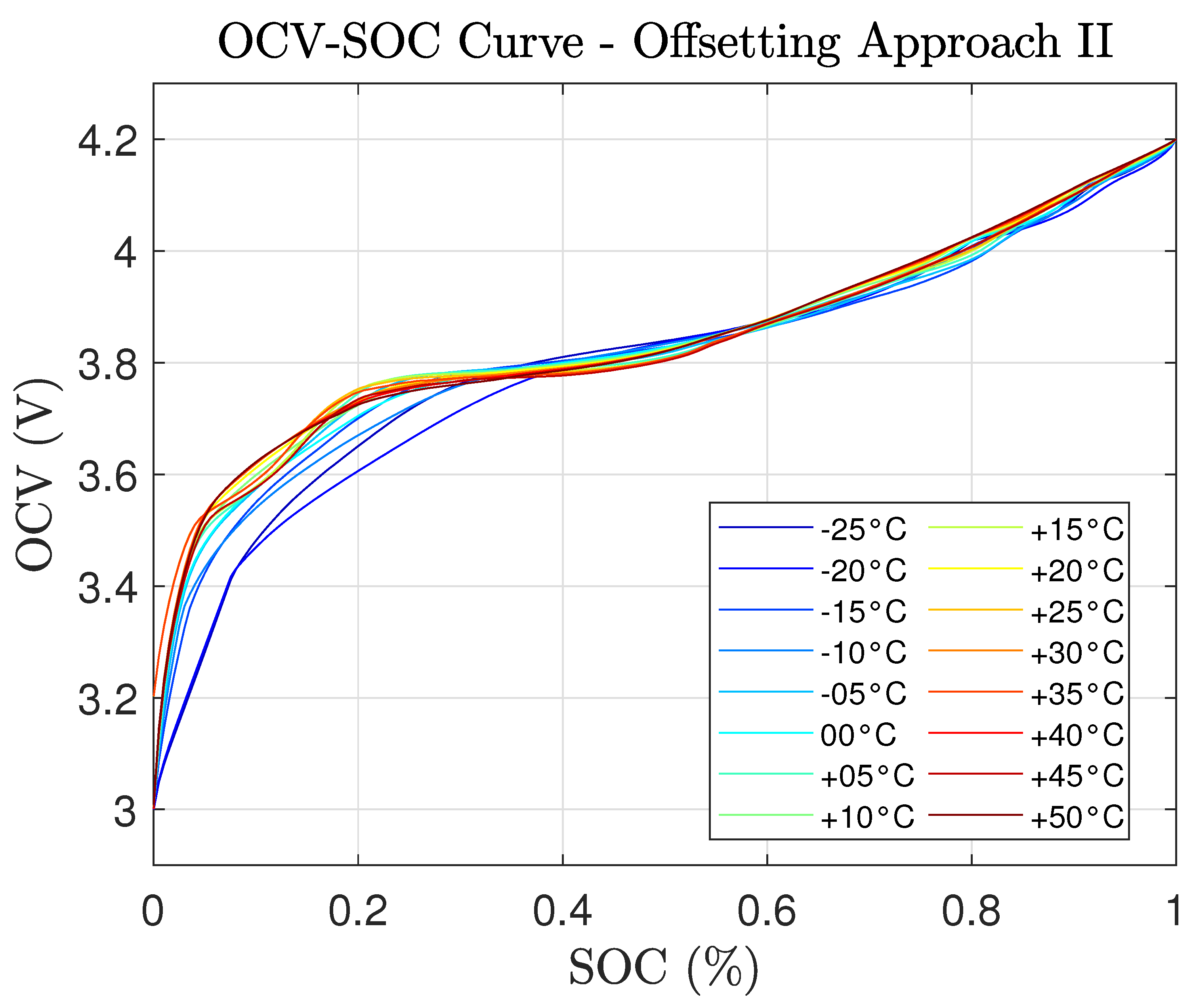
Figure 9.
Comparison between Offsetting Approach I and II.
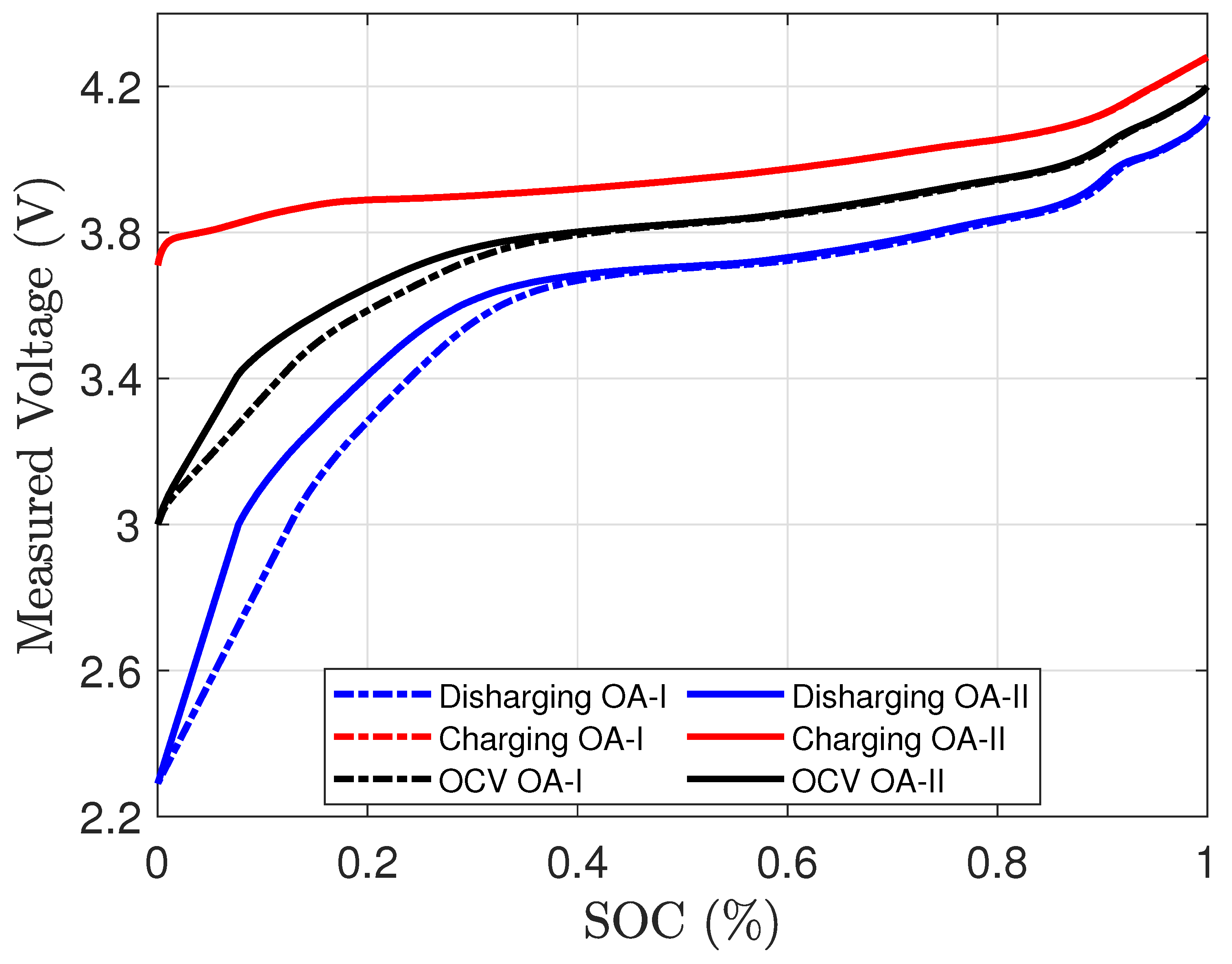
Figure 10.
R-int model
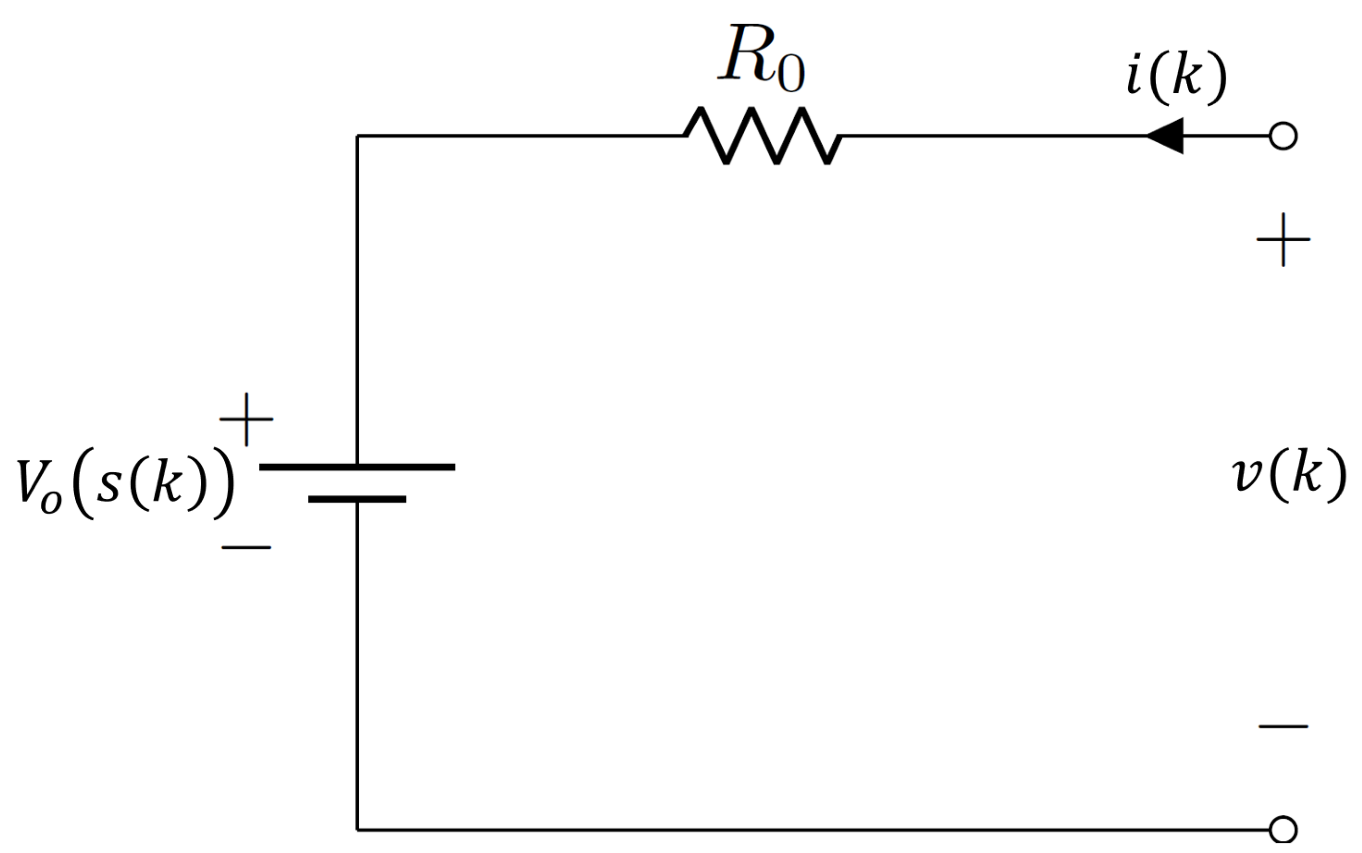
Figure 11.
Battery Simulator Flow Chart.
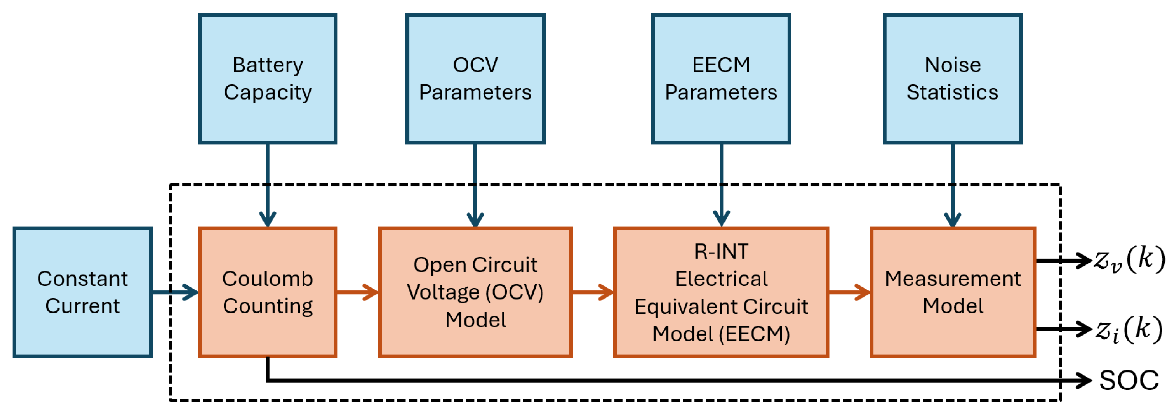
Figure 12.
Simulation of identical Li-on battery with varying resistances
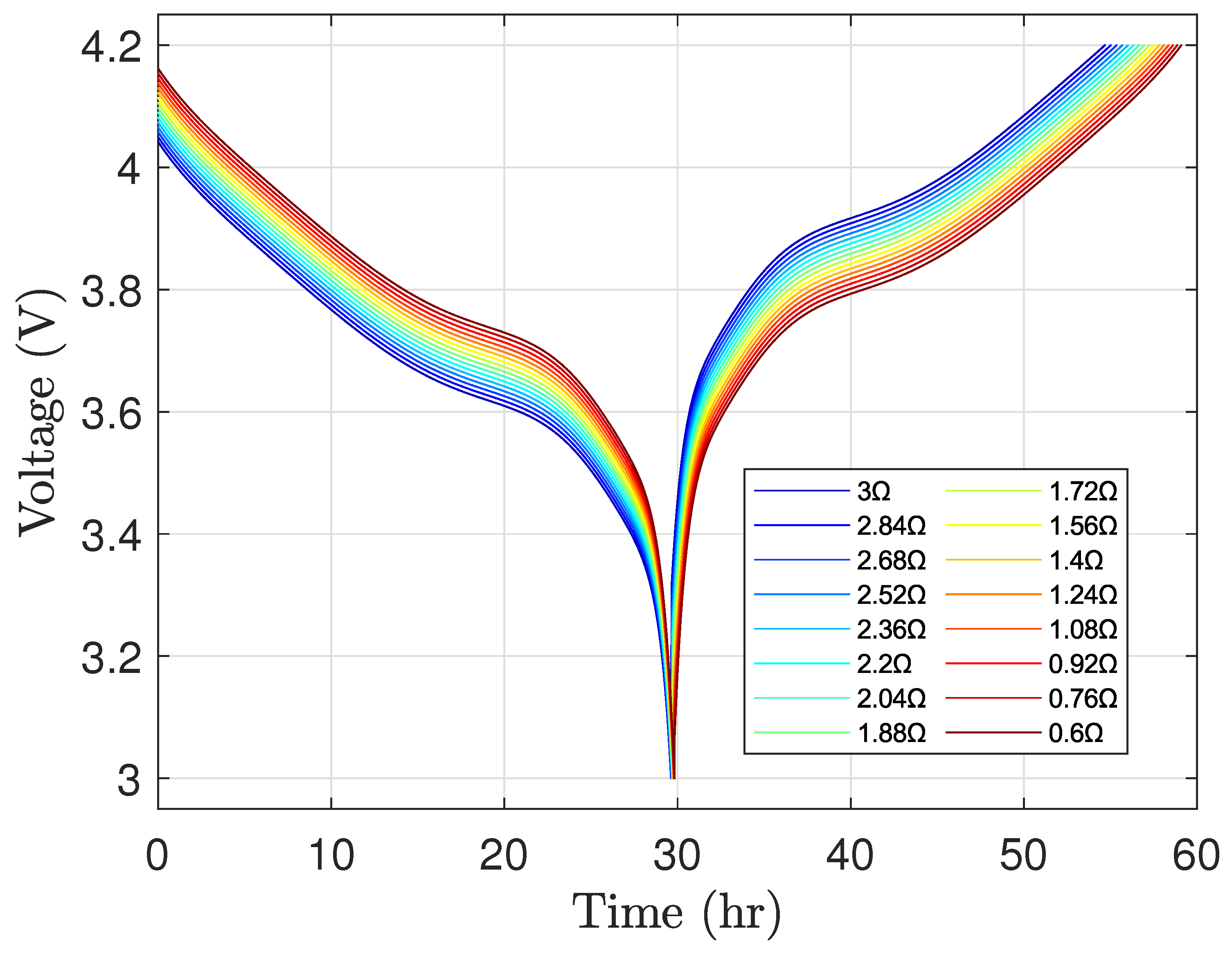
Figure 13.
Simulated Terminal Voltages during Low-rate OCV test.
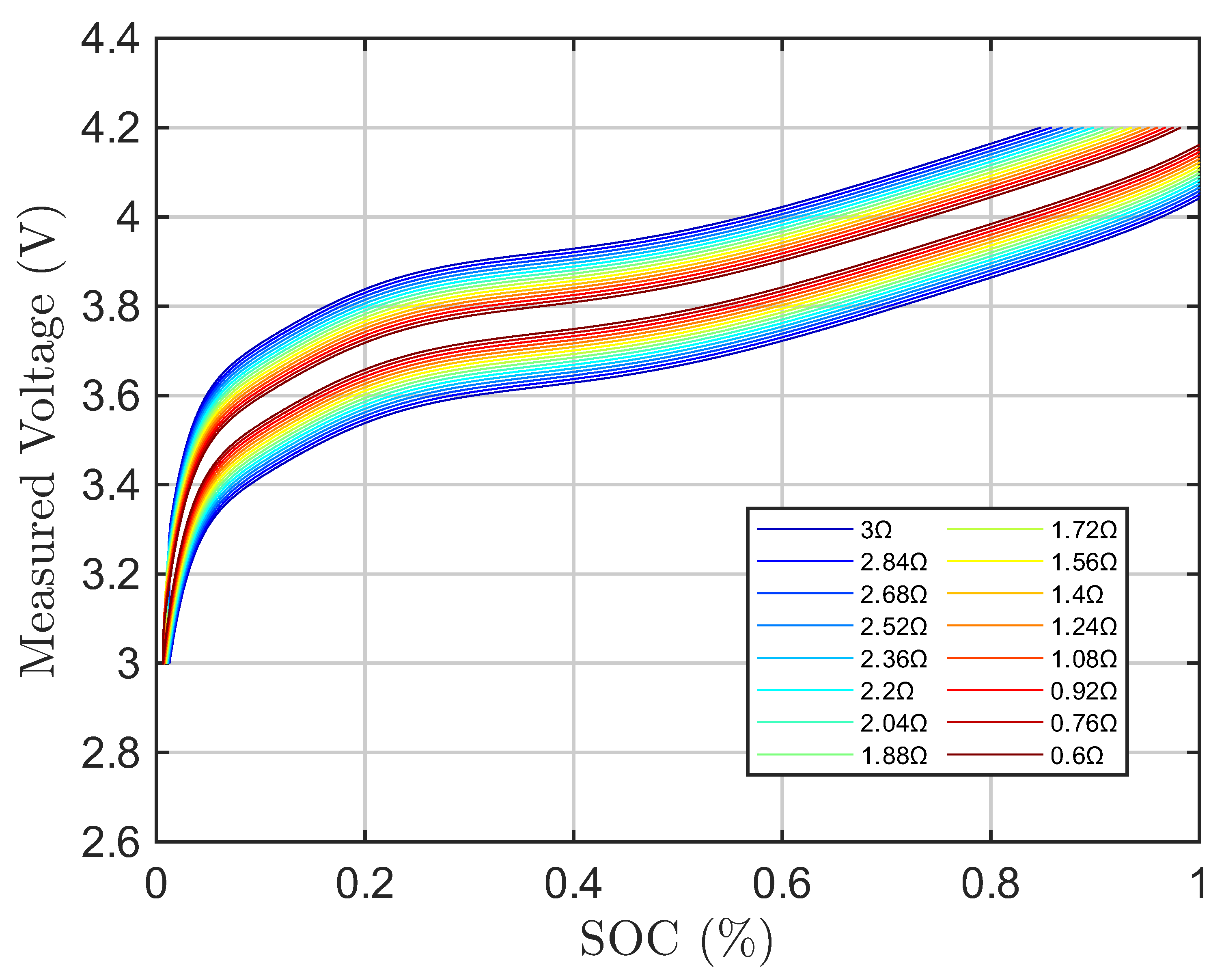
Figure 14.
Simulated Normalized Terminal Voltages during Low-rate OCV test.
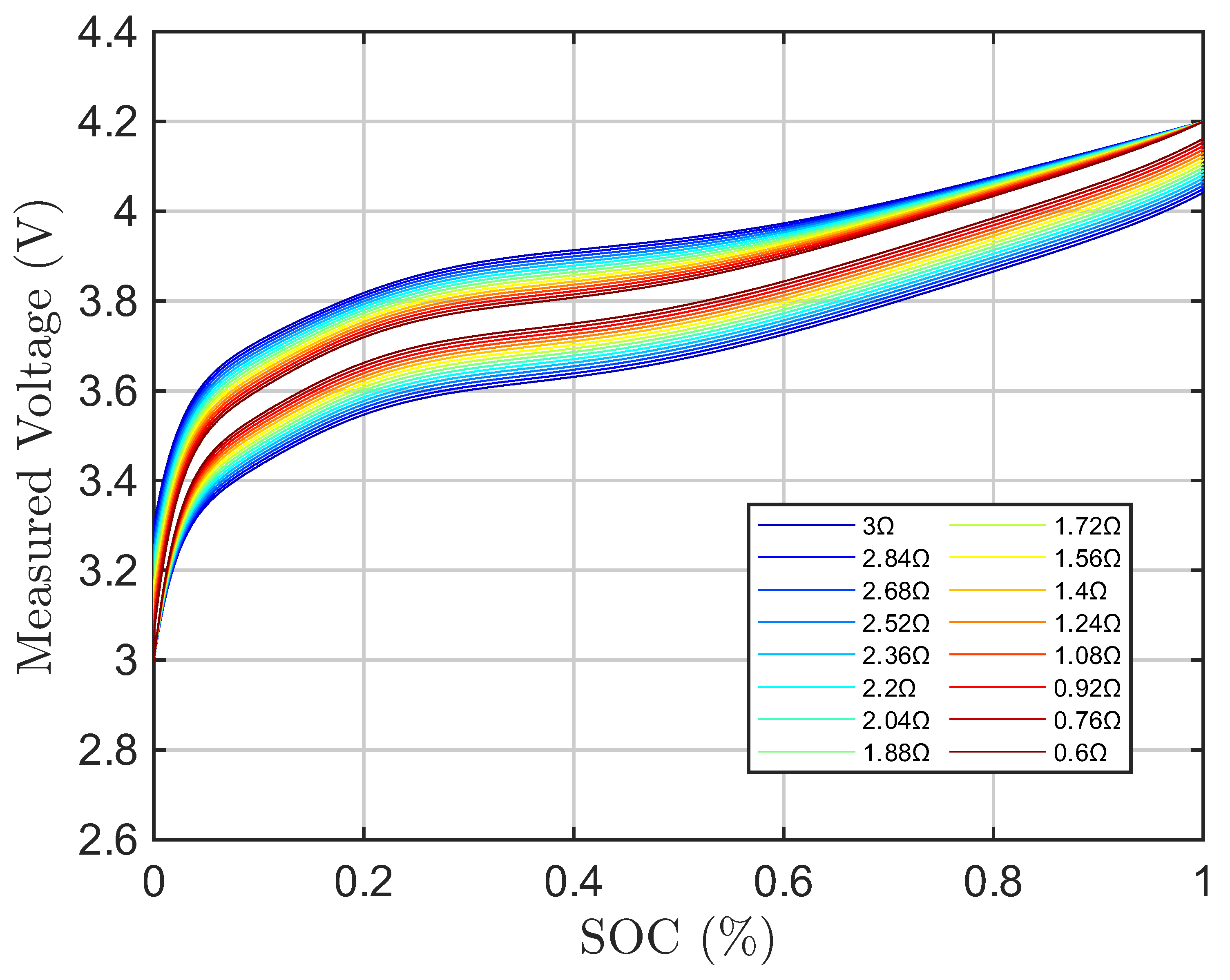
Figure 15.
OCV-SOC curve of simulated battery with varying resistances.
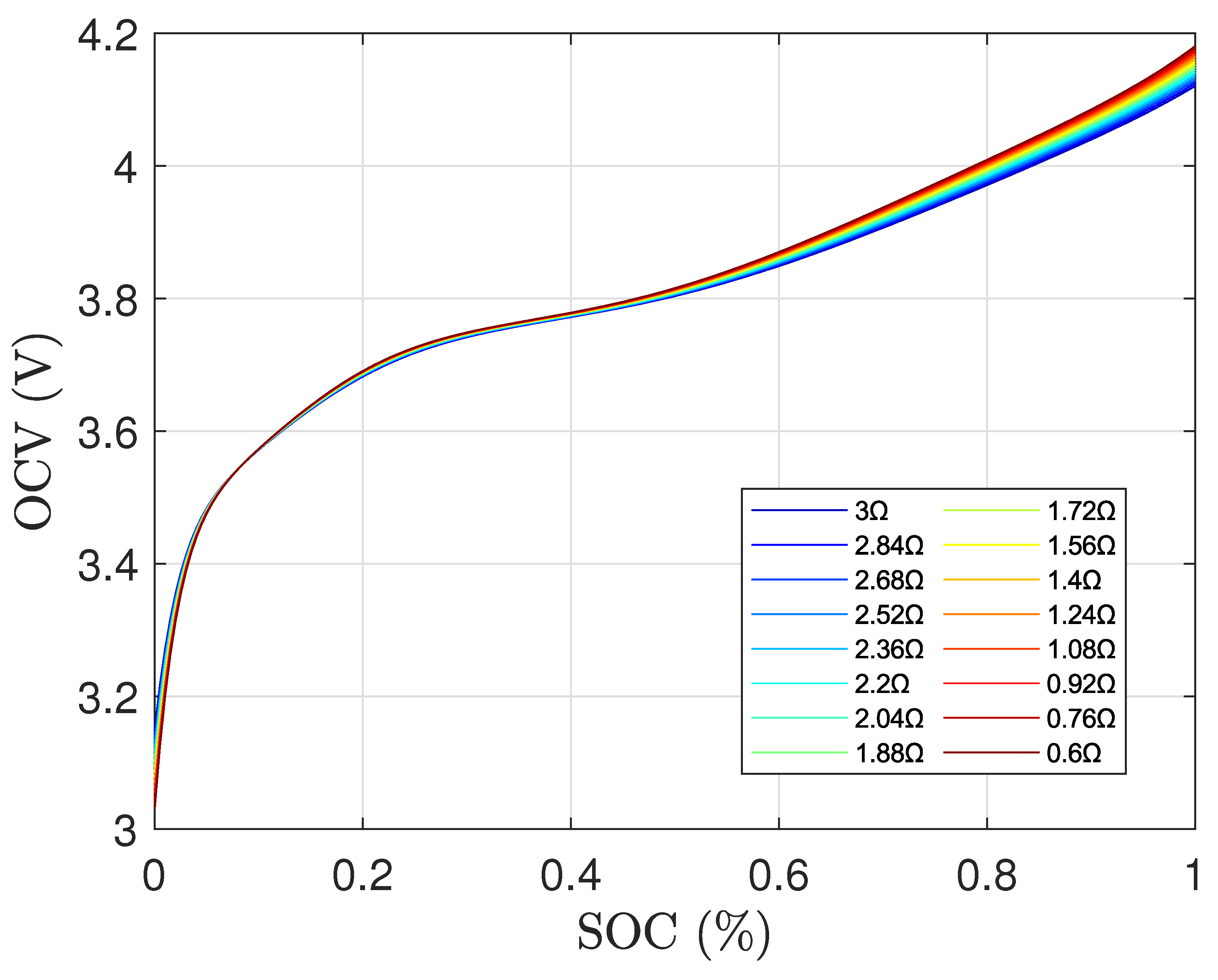
Figure 16.
OCV-SOC curve of simulated battery with varying resistances.
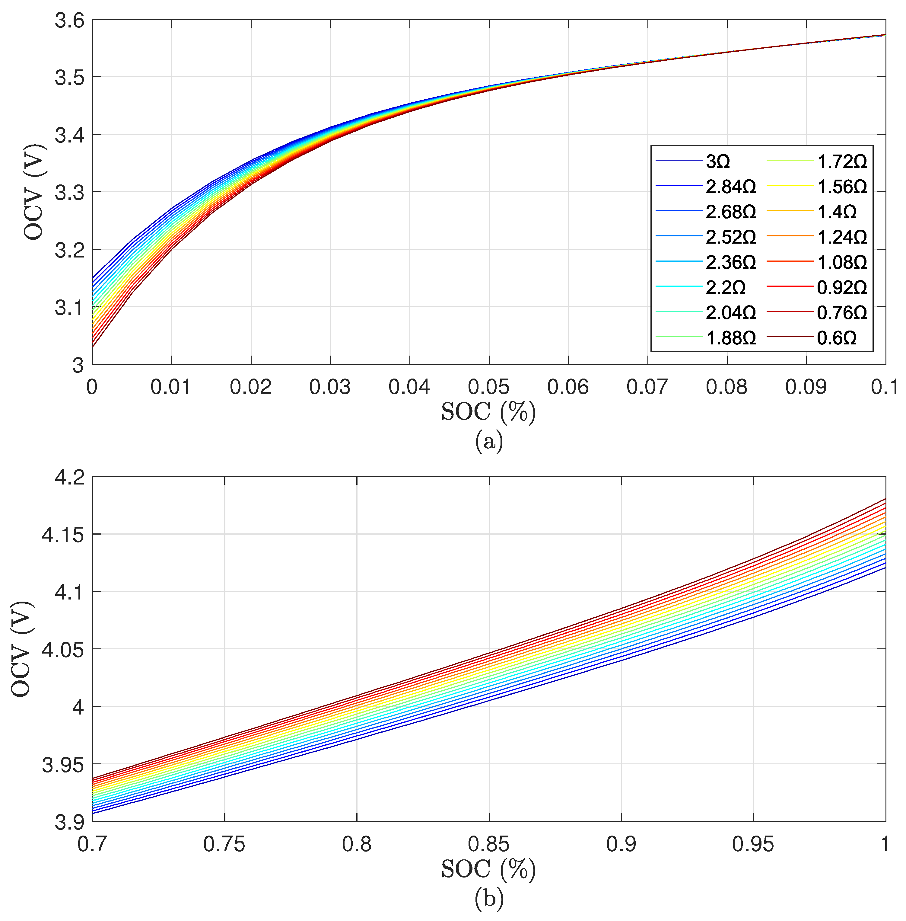
Figure 17.
Proposed Offsetting Approach applied on simulation of identical Li-on battery with varying resistances.
Figure 17.
Proposed Offsetting Approach applied on simulation of identical Li-on battery with varying resistances.
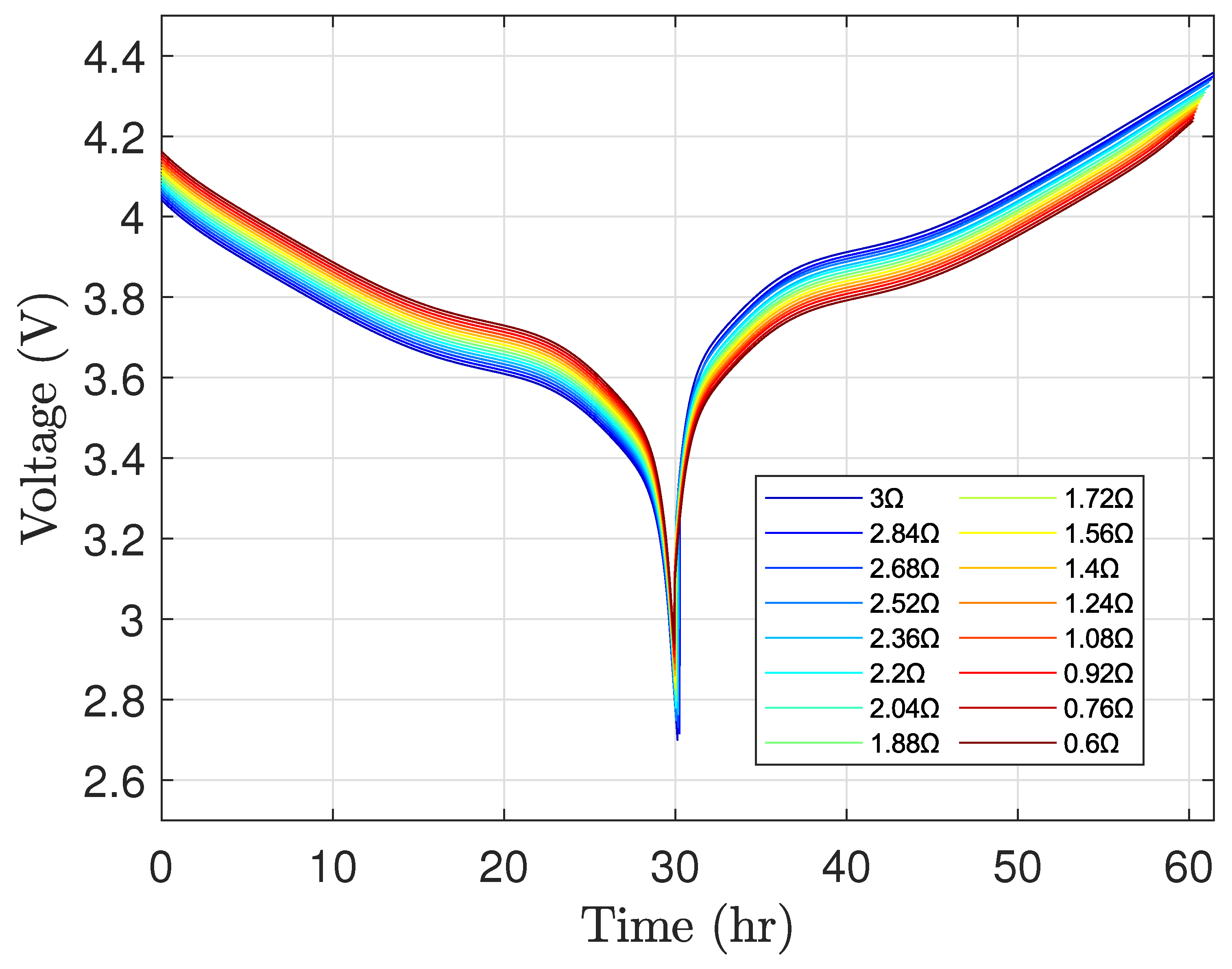
Figure 18.
Proposed Offsetting Approach OCV-SOC Curves.
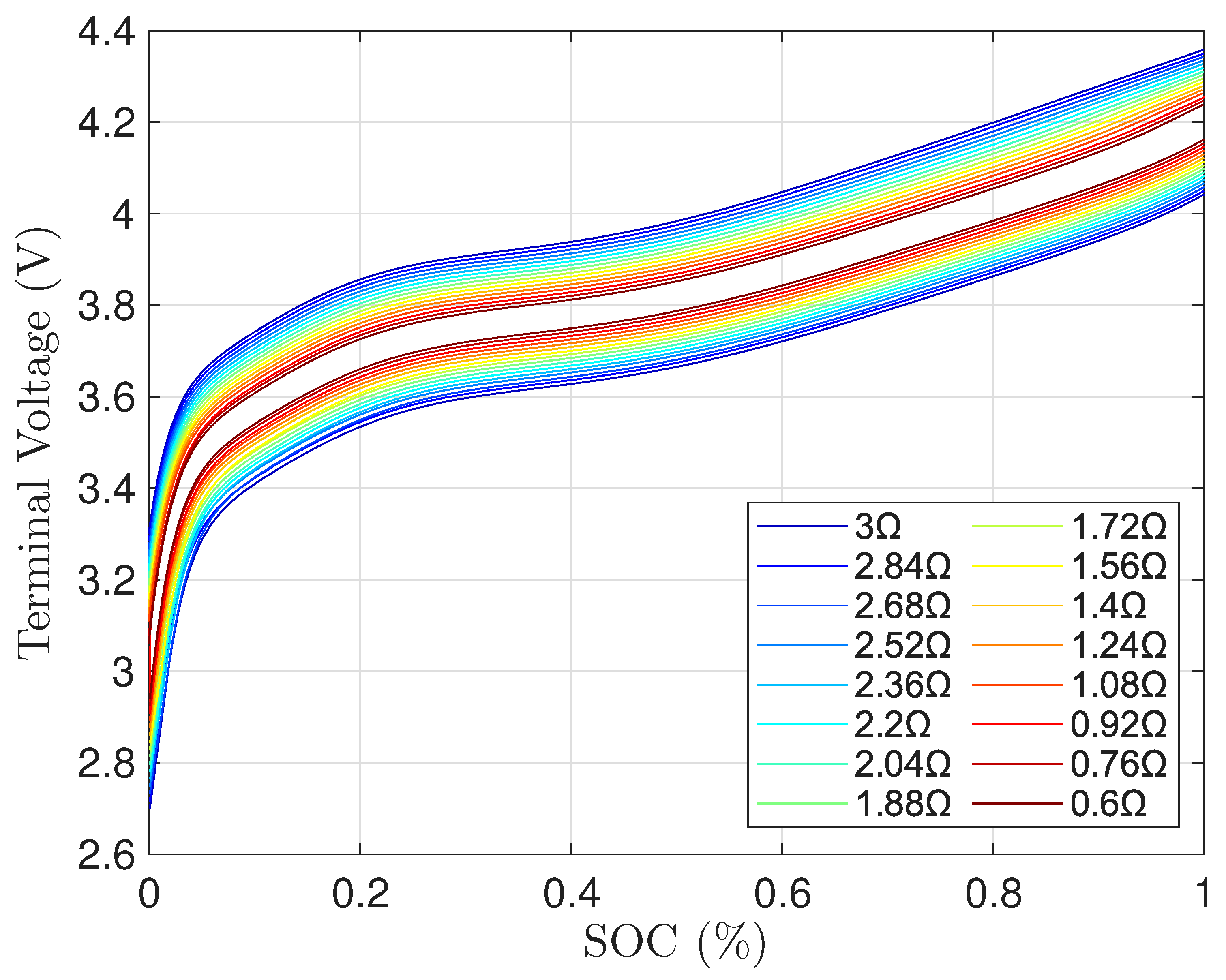
Figure 19.
OCV-SOC curve of Proposed Offsetting Approach.
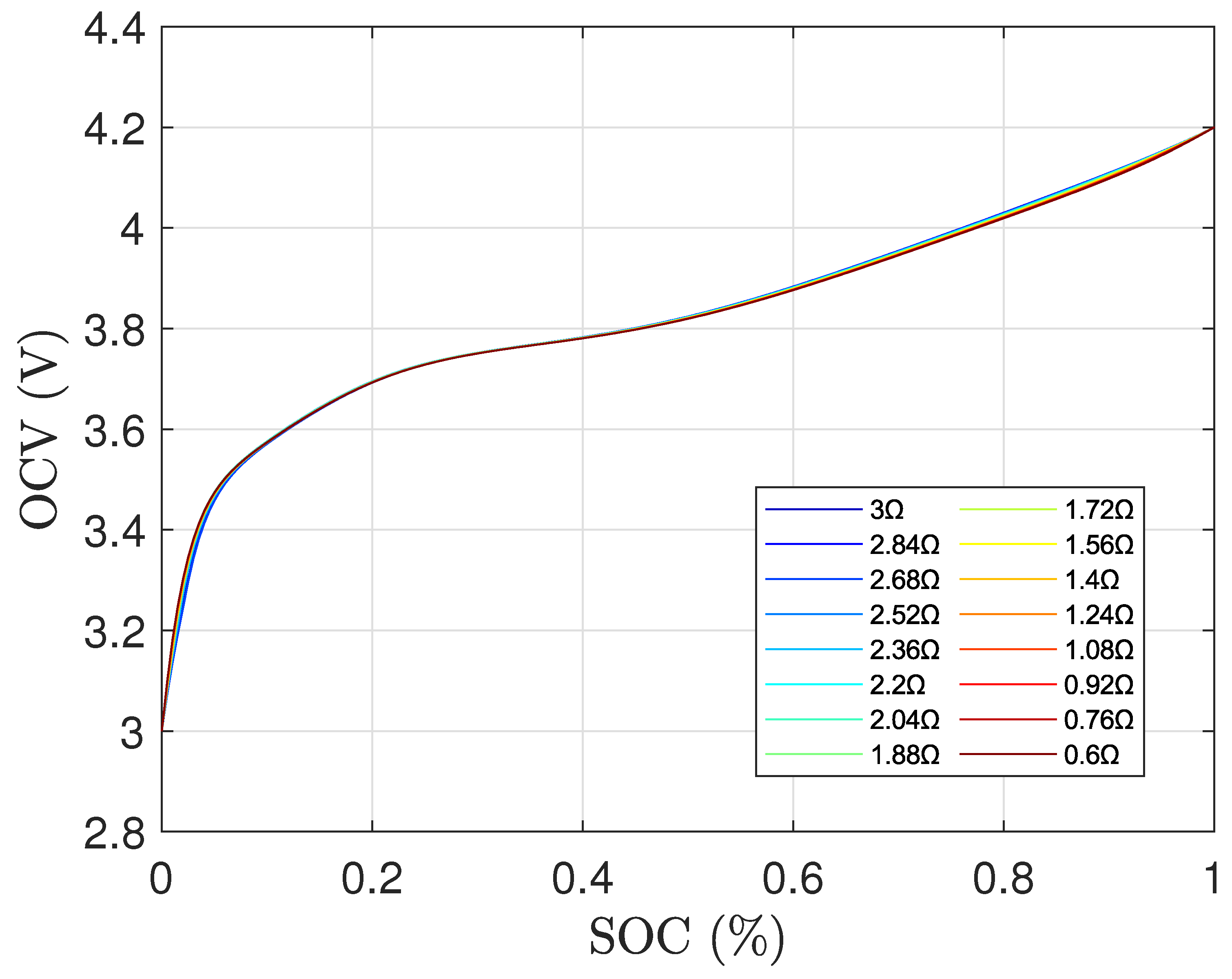
Figure 20.
Cell to Cell Variation vs SOC for Traditional low-rate OCV Approach (a) and Proposed Offsetting Approach (b).
Figure 20.
Cell to Cell Variation vs SOC for Traditional low-rate OCV Approach (a) and Proposed Offsetting Approach (b).
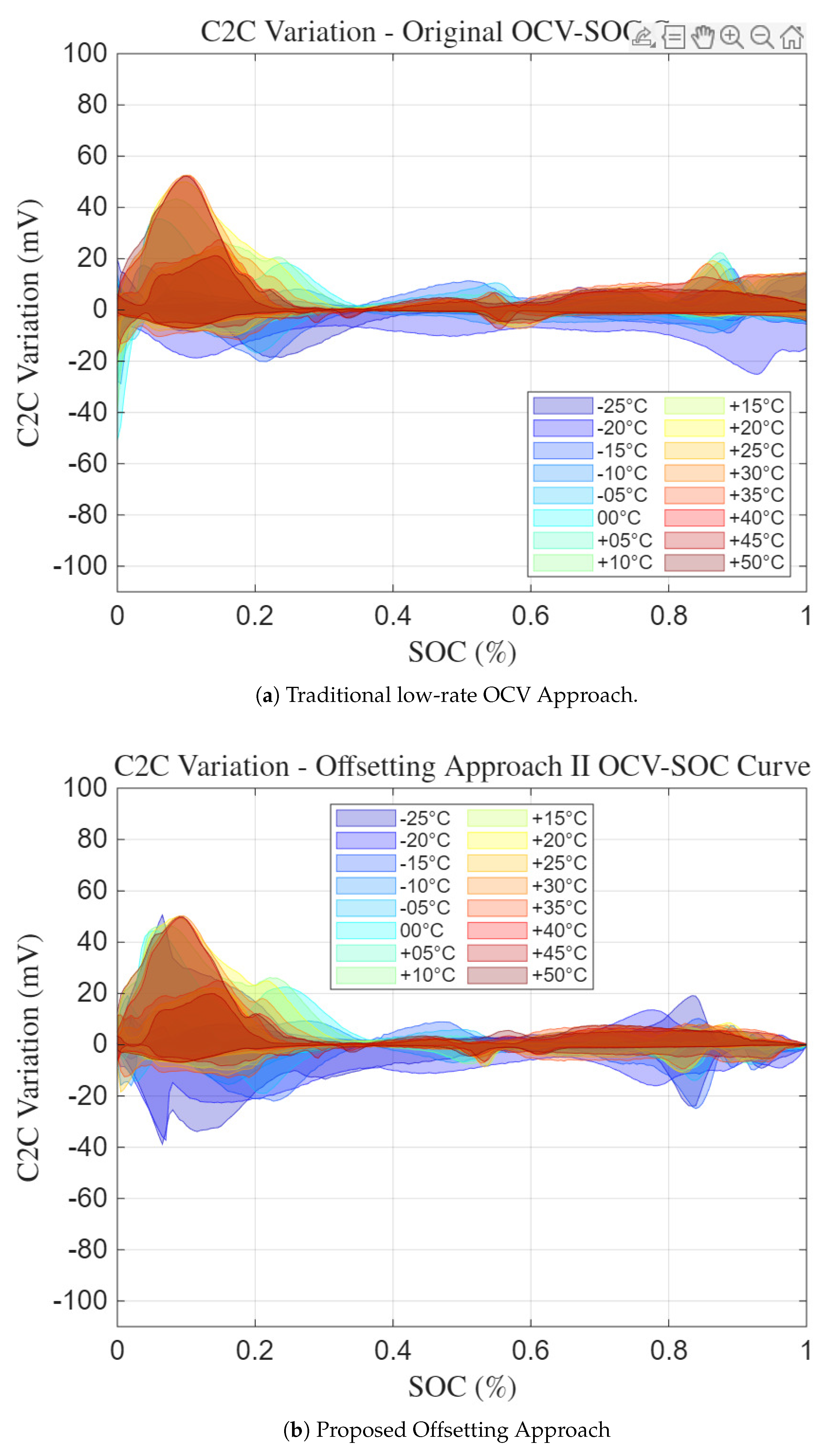
Figure 21.
Temperature Variation at the extreme temperatures for both approaches.
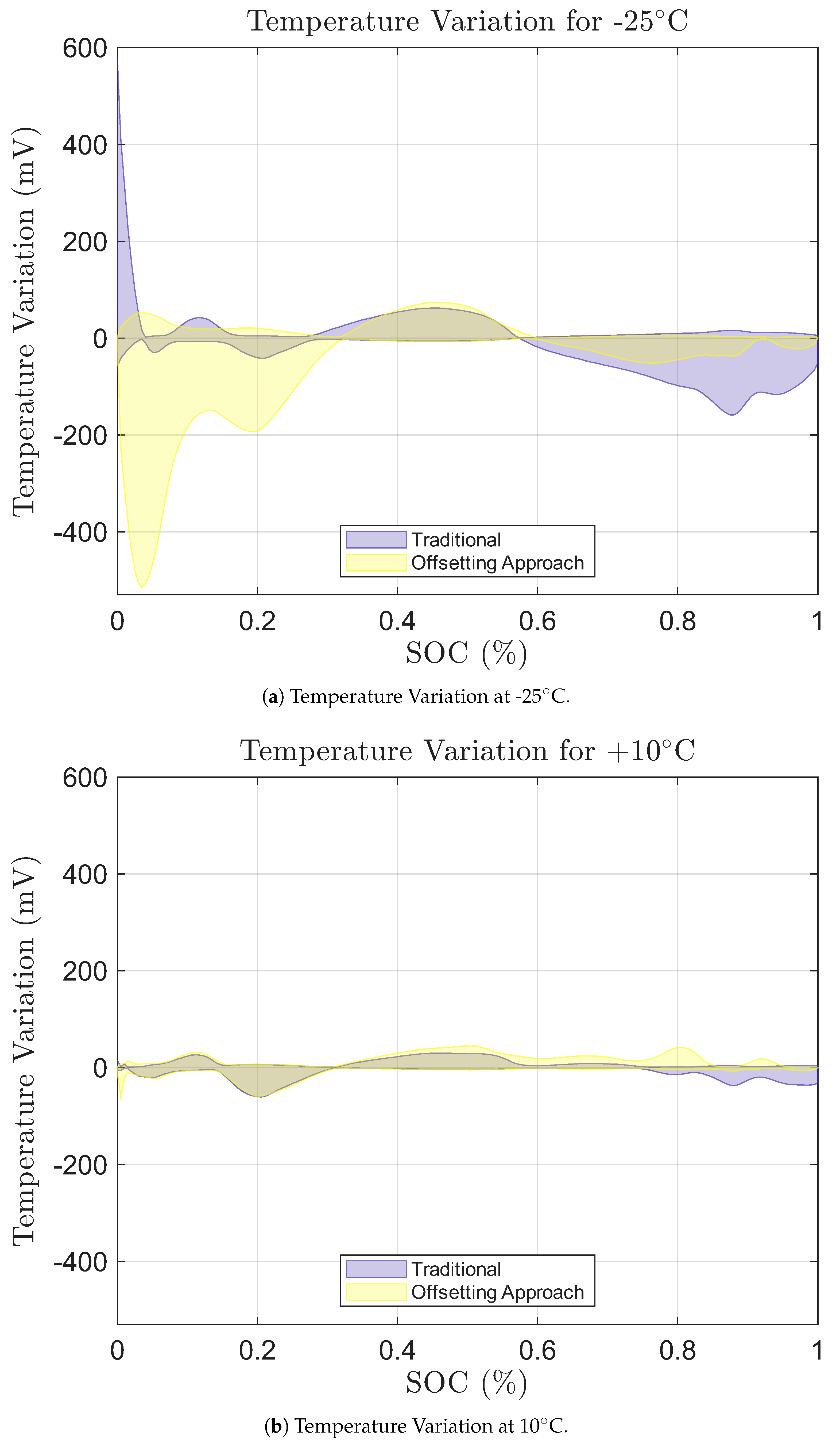
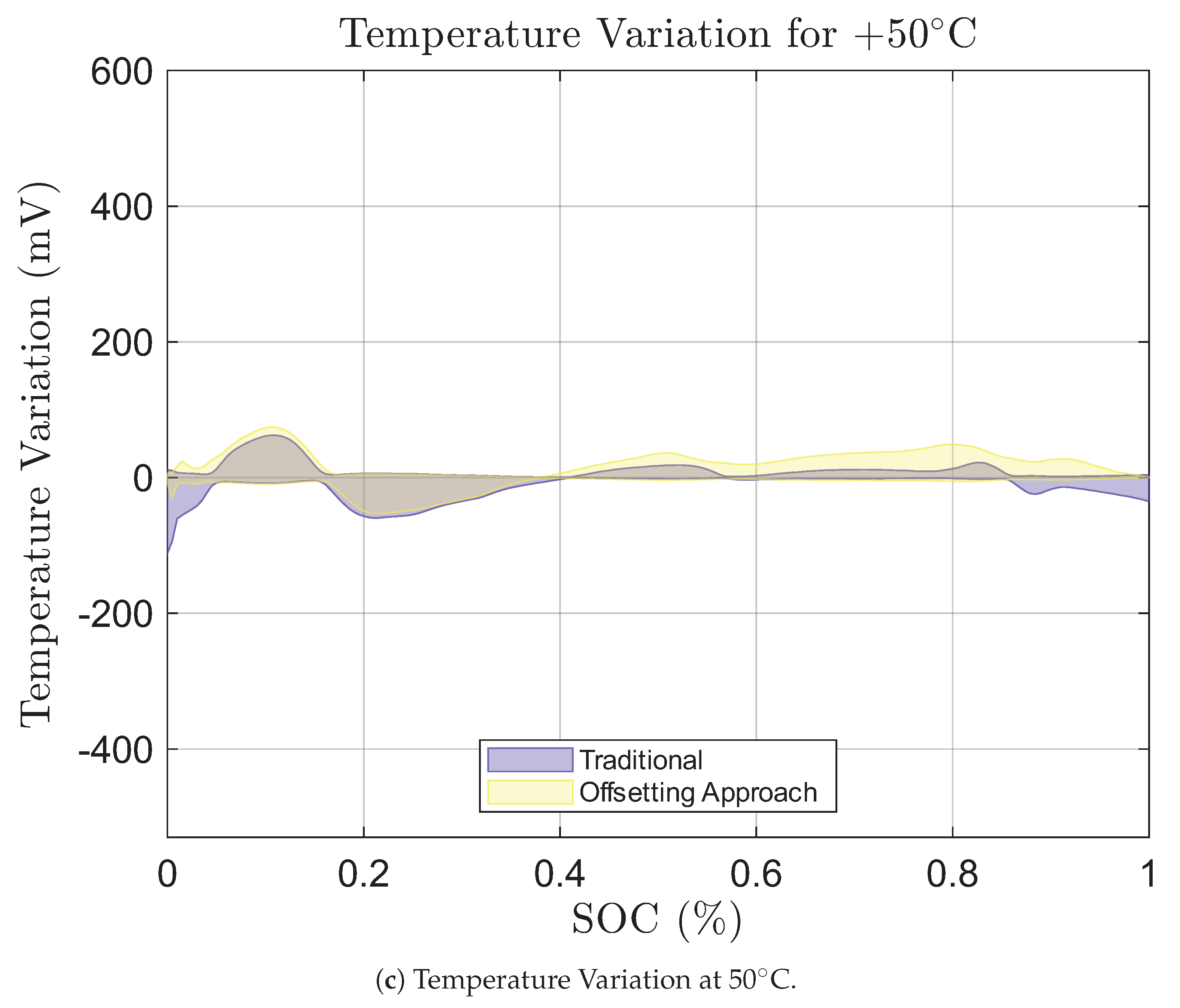
Figure 22.
Temperature Variation vs SOC for both Offsetting Approaches for Traditional low-rate OCV Approach (a) and Proposed Offsetting Approach (b).
Figure 22.
Temperature Variation vs SOC for both Offsetting Approaches for Traditional low-rate OCV Approach (a) and Proposed Offsetting Approach (b).
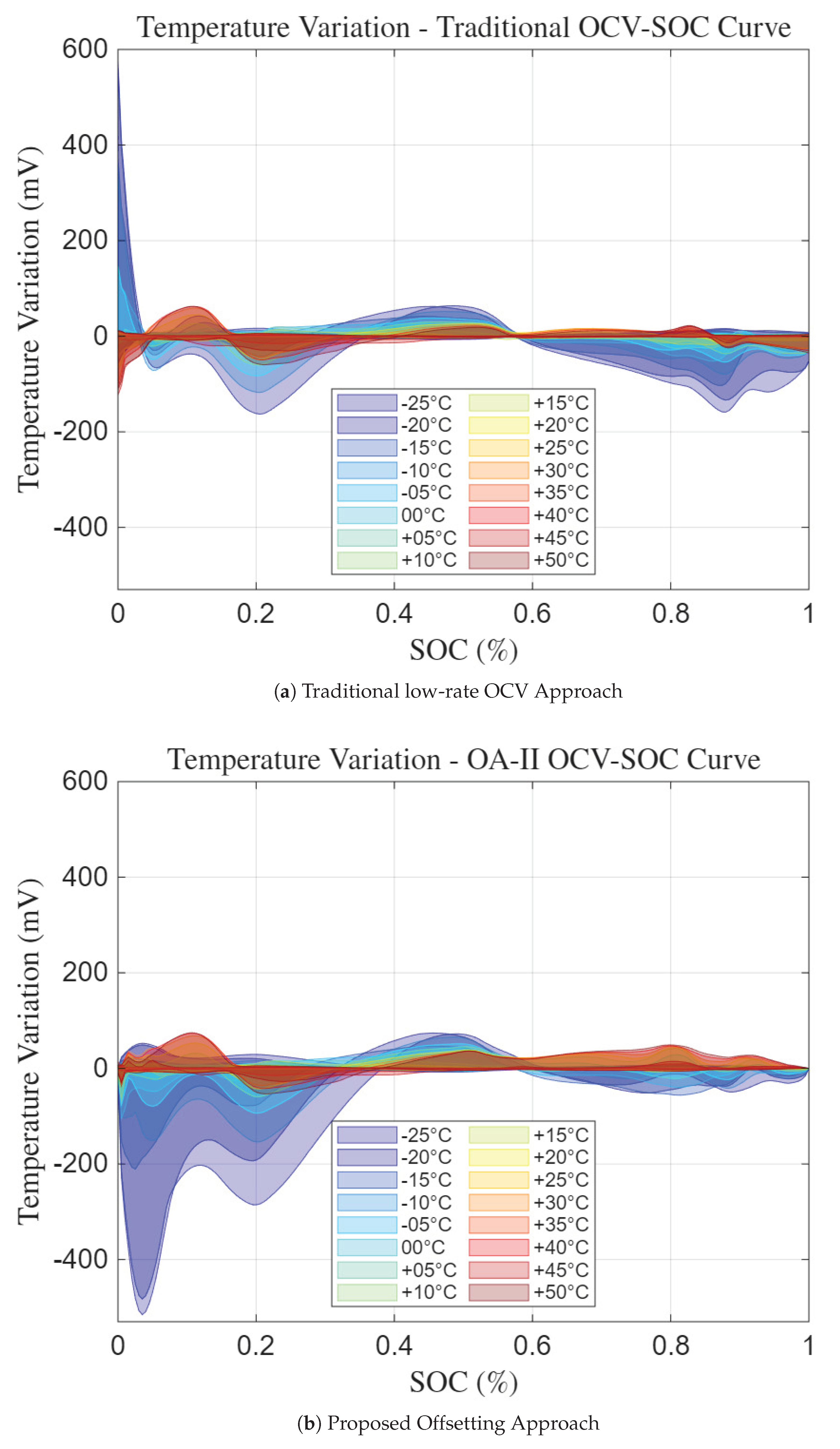

Table 1.
Temperature and Resistance Correlation.
| Temperature (∘C) | Resistance () |
|---|---|
| -25 | 3.00 |
| -20 | 2.84 |
| -15 | 2.68 |
| -10 | 2.52 |
| -05 | 2.36 |
| 00 | 2.20 |
| +05 | 2.04 |
| +10 | 1.88 |
| +15 | 1.72 |
| +20 | 1.56 |
| +25 | 1.40 |
| +30 | 1.24 |
| +35 | 1.08 |
| +40 | 0.92 |
| +45 | 0.76 |
| +50 | 0.60 |
Table 2.
OCV data for all temperatures and batteries.
| Temp No. | OCV (cell 1) | OCV (cell 2) | ... | OCV (cell ) |
|---|---|---|---|---|
| 1 | ... | |||
| 2 | ... | |||
| ⋮ | ⋮ | ⋮ | ⋮ | ⋮ |
| ... |
Table 3.
Low-end and High-end mean error metric.
| Temp No. | ||
|---|---|---|
| 1 | ||
| 2 | ||
| ⋮ | ⋮ | ⋮ |
Table 4.
C2C mean and standard deviation error metric.
| Temp No. | ||
|---|---|---|
| 1 | ||
| 2 | ||
| ⋮ | ⋮ | ⋮ |
Table 5.
Temperature mean and standard deviation error metric.
| Temp No. | ||
|---|---|---|
| 1 | ||
| 2 | ||
| ⋮ | ⋮ | ⋮ |
Table 6.
Low-End Offset of each temperature.
| Temperature (∘C) | OCV at (V) | |
|---|---|---|
| -25 | 3.3476 | 0.34758 |
| -20 | 3.3412 | 0.3412 |
| -15 | 3.2558 | 0.25575 |
| -10 | 3.2385 | 0.23852 |
| -05 | 3.1561 | 0.15607 |
| 00 | 3.1545 | 0.15447 |
| +05 | 3.0937 | 0.093667 |
| +10 | 3.093 | 0.092967 |
| +15 | 3.0564 | 0.0564 |
| +20 | 3.06 | 0.059967 |
| +25 | 3.2296 | 0.088667 |
| +30 | 3.0452 | 0.045217 |
| +35 | 3.2251 | 0.088004 |
| +40 | 3.0403 | 0.040283 |
| +45 | 3.0334 | 0.033367 |
| +50 | 3.0385 | 0.03855 |
Table 7.
High-End Offset of each temperature.
| Temperature (∘C) | OCV at (V) | |
|---|---|---|
| -25 | 4.1596 | 0.040417 |
| -20 | 4.16 | 0.04005 |
| -15 | 4.1746 | 0.0254 |
| -10 | 4.1702 | 0.0298 |
| -05 | 4.181 | 0.01895 |
| 00 | 4.1691 | 0.030933 |
| +05 | 4.1812 | 0.0188 |
| +10 | 4.1685 | 0.03155 |
| +15 | 4.1789 | 0.021067 |
| +20 | 4.1719 | 0.02805 |
| +25 | 4.1826 | 0.01735 |
| +30 | 4.1714 | 0.02865 |
| +35 | 4.1819 | 0.018133 |
| +40 | 4.1693 | 0.030667 |
| +45 | 4.182 | 0.018 |
| +50 | 4.1671 | 0.032883 |
Disclaimer/Publisher’s Note: The statements, opinions and data contained in all publications are solely those of the individual author(s) and contributor(s) and not of MDPI and/or the editor(s). MDPI and/or the editor(s) disclaim responsibility for any injury to people or property resulting from any ideas, methods, instructions or products referred to in the content. |
© 2025 by the authors. Licensee MDPI, Basel, Switzerland. This article is an open access article distributed under the terms and conditions of the Creative Commons Attribution (CC BY) license (http://creativecommons.org/licenses/by/4.0/).
Copyright: This open access article is published under a Creative Commons CC BY 4.0 license, which permit the free download, distribution, and reuse, provided that the author and preprint are cited in any reuse.


