
Submitted:
29 October 2025
Posted:
30 October 2025
You are already at the latest version
Abstract
The concept of correlation appears straightforward: measurement outcomes coincide, and patterns emerge. For any record of events, the coefficients are uniquely determined. Thus, if correlations change spontaneously, as seen in quantum monogamy, then individual behavior must have changed first. Surprisingly, this is not always true. When two observables are mutually exclusive, they cannot coincide objectively and need to be grouped across time. Yet, sectioning the flow of events into “iterations” is not trivial in this case. Even with blind windows of coincidence, the same order of outcomes can produce different coefficients of correlation, depending on the number of joint measurements. Therefore, quantum monogamy can happen with fixed pre-determined events. This discovery has wide implications, closing the gap between quantum and classical probability.
Keywords:
quantum correlations
; quantum monogamy
; probability theory
; unification
1. Introduction
Quantum entanglement is famous for its interpretive paradoxes, but the theoretical puzzles are no less challenging. Quantum theory predicts violations of Bell’s inequality, but also the disappearance of such violations for triple or quadruple joint measurements. This is one aspect of the so-called “quantum monogamy” [1,2,3,4,5,6]. The coefficient of correlation between two observables can change spontaneously, just because another remote property is detected at the same time. An important nuance here is that quantum correlations are fundamentally different from classical correlations. Incompatible quantum coefficients do not express conditional sub-ensembles from a full record of events. Instead, different bases of measurement lead to different predictions for the same wavefunction. Thus, quantum monogamy cannot be dismissed as a mere artifact of post-selection, for example by assuming that triple coincidences are less likely than double coincidences [7]. Quantum predictions hold for ideal measurements, with no event loss [8]. So, how is this possible? It is tempting to jump to ontological conclusions, but have we reached the limits of probability theory? In other words, is it a fact that fluid coefficients cannot emerge from a fixed record of events?
As will be shown below, the answer is negative. In a way, the solution was “too obvious” to be seen before. Non-commuting variables are mutually exclusive. They correspond to properties that exist one at a time and therefore cannot coincide. Joint observations require operations across contexts, and sometimes across systems, with unavoidable conditional effects. This process is illustrated below with a “wheel of fortune” correlation thought experiment. The same record of fixed events produces two types of coefficients automatically, depending on the number of variables that are observed in the same window. Maximal Bell violations are achieved in pairwise joint measurements, but no violations are possible with quadruple measurements. This result demystifies the nature of quantum monogamy, with deep implications about quantum correlations in general (see the Discussion section, as well as the Appendix at the end).
2.“. Wheel-of-Fortune” Thought Experiment
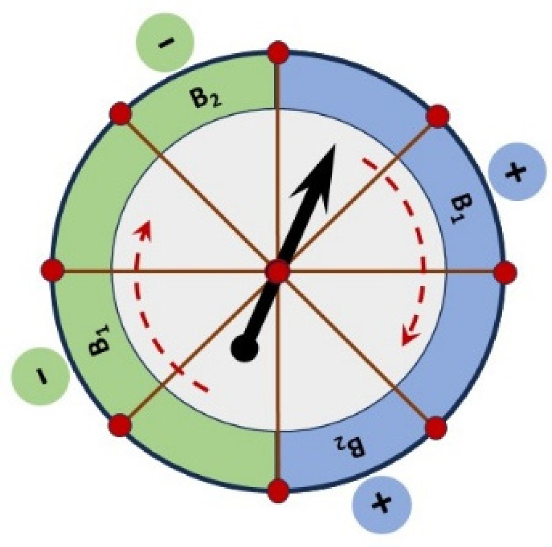
A big difficulty in the analysis of quantum experiments is that we don’t know what is going on. Do we measure properties that exist all at the same time, or one at a time? Do we have predetermined fixed events, or spontaneous manifestations? The advantage of a thought experiment is that such uncertainties can be removed by design. So, let us consider a system that is classical in every way, except that all the properties exist one at a time. To be clear, this is not like a system with four lights, where one light is always “on”, and the other ones are “off”. The correct analogy is a system that “shape-shifts” continuously, morphing sequentially into four different types of light emitters, one at a time. This is represented below with a “wheel-of-fortune” table that has a fixed order of manifestation for four properties (Figure 1). It contains a closed cycle of 8 sectors, with four positive and four negative values. As the table spins under the arrow, only one sector is “actualized” at a time and is recorded as an event within a well-defined time interval. Therefore, joint observations for two properties can only be achieved across time, with extended windows of coincidence. Note that printed values are fixed and cannot influence each other. It makes no difference if “Alice” and “Bob” events are on the same table, or on two identical tables. The advantage of a single table, as shown below, is that the relationship between events and correlations can be explored with visual clarity.
A CHSH-type experiment [9] requires four binary observables: A1, A2, B1 and B2. The goal is to make a closed chain of overlapping joint measurements: (A1,B1) – (B1,A2) – (A2,B2) – (B2,A1). As shown in Figure 1, this can be achieved by assigning dedicated axes with opposite values to each variable. “Alice” and “Bob” values are interlaced, such that any “Alice” event is placed between two different “Bob” events. An open question is whether a Bell violation is possible with pairwise consistency, such that the marginals of (A1,B1) and (B1,A2) always agree about the values of B1, and so on around the chain. This can be achieved by default in this case, given the fixed sequence of predetermined values on the table. At the same time, event pairings cannot be random. The goal is to achieve the strongest possible correlations. This requirement is satisfied by placing all the positive-valued sectors on one half of the table, with the negative values on the other half. The table can be forced to rotate with constant speed, such that a fixed window of coincidence can always isolate joint observations from the recorded flow of events.
The most important feature of this system is that only one sector can be “real” (i.e., pass under the arrow), at any point in time. This makes it impossible to have objective coincidences. This is why joint measurements require extended windows of observation. The width of the window of coincidence can be adjusted as necessary, to include two consecutive events or more. Furthermore, quantum measurements require preparation procedures. Here, the spinning table works as a mechanism with automatic sequential “preparations”, such that any property can only manifest “when prepared”, i.e., when it gets a turn. The same cycle of events is repeated continuously, as long as needed for statistical significance. This makes it easy to infer the patterns of possible coincidence, since the sequence of measurement outcomes cannot change over time.
3.“. Quantum Monogamy” with Fixed Measurement Outcomes
In a system with sequential properties, all the variables can have an equal chance of manifestation, in order. In this case, for every complete turn of the “wheel-of-fortune”, every variable is expressed twice. Positive values for A1-B1-A2-B2 are followed by negative values in the same order. This means that a joint measurement of the four variables requires a window of coincidence that is equal to half the period of rotation. In principle, this procedure can be repeated indefinitely for data acquisition. Yet, the cyclic nature of this process entails a stable pattern of coincidence, with one possible actualization as shown in Figure 2(a). A complete record of events will have only two types of coincidences. Half the iterations will have positive events exclusively, as represented by the inner circle in the diagram. The other half will have negative values, as represented by the outer circle.
Thus, no further analysis is needed to derive the four pairwise correlations for a CHSH test. The only possible combinations of events for the pair (A1,B1) are “+,+” and “-,-”. The expectation value is E(A1,B1)=1. The same pattern holds for all the remaining pairwise combinations in the Bell chain. Accordingly, we can plug these coefficients into the CHSH inequality [9]:
|E(A1,B1) ̶ E(A1,B2) + E(A2,B1) + E(A2,B2)| ≤ 2.
The result is a confirmation of the expected “classical” limit:
S= | 1 – 1 + 1 + 1 | = 2.
What happens if the window of coincidence is narrow enough to include only two events at a time? In this case, a full turn of the table corresponds to a double loop of a Mobius strip, as shown in Figure 2(b). Instead of batches of four events, where pairwise coincidences are extracted from within quadruple observations, we have a continuous suite of overlapping pairwise measurements. Surprisingly, this results in a “non-classical” combination of three correlations and one anti-correlation. Coincidences for (A1,B1), (B1,A2) and (A2,B2) remain the same as in the previous example, with nothing but “+,+” and “-,-” pairings. Therefore, they still have an expectation value of (+1). In contrast, coincidences between A1 and B2 happen across the two halves of the table (Figure 1), corresponding to the area with cross-overs between the loops of the Mobius strip in Figure 2(b). The only possible combinations in this case are “+, -” and “-,+”, with an expectation value of (-1). If these values are plugged into the CHSH inequality, we get a maximal Bell violation:
S = | 1 – ( – 1) + 1 + 1 | = 4.
The same flow of events produces two different combinations of expectation values, just as observed in the case of “quantum monogamy”. The only difference is that Bell violations are maximal in this case, leading to a general conclusion. Any kind of “monogamy” phenomena can be explained (at least in principle) with a fixed record of events.
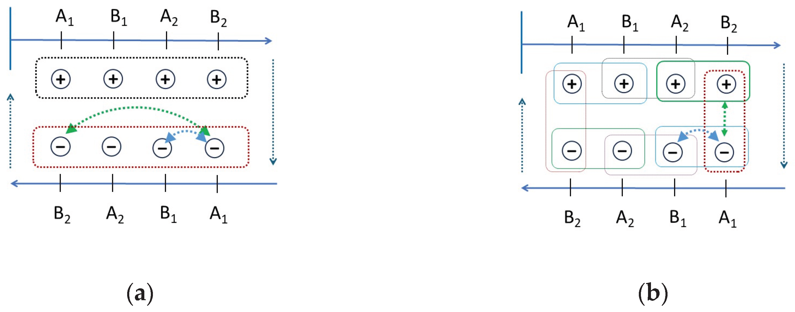
As shown in Figure 3 below, this is a straightforward combinatorial effect. When all the properties are measured in a single window of coincidence, the flow of events is broken into non-overlapping batches of four events (Figure 3a). Every event is used twice, as required for a local Bell experiment. However, the values of A1 are not paired with the closest manifestation of B2. Instead, they are paired with a remote value of B2 from the same coincidence window. In contrast, the narrower window of coincidence results in a continuous chain of overlapping pairwise measurements (Figure 3b). This means that A1 and B2 values are always grouped with the values that are closest in time to each other. Accordingly, switching from a quadruple joint measurement scheme to a double joint measurement scheme entails an unavoidable flip for just one out of four expectation values. This is enough to change the outcome of a CHSH calculation from a non-violation to a maximal violation.
To sum up, mutually exclusive properties do not coincide objectively and require artificial grouping. This process is sensitive to the number of variables that are combined into joint measurements, such that pairwise observations allow for Bell violations, while global observations do not. A fixed record of detection events is compatible with both patterns of coincidence that are associated with the so-called “quantum monogamy” phenomenon. This is only possible for mutually exclusive properties. Though, quantum theory is only known to predict this behavior for non-commuting variables. Therefore, this demonstration is sufficient to falsify the need for “new physics” as an interpretive resource for unusual quantum correlations.
4. Discussion
Quantum correlations do not have analogues in classical probability theory. The current attitude is that non-classical physical mechanisms are required for such patterns. Yet, there is a mismatch between classical probability theory and classical physics. Kolmogorov-type families of variables are restricted to jointly distributed configurations. This corresponds to predetermined properties that manifest at the same time. However, it is logically possible for predetermined properties to also occur at different times. For example, a set of mutually exclusive properties can manifest sequentially, in a pre-defined order. Similarly, some systems could experience mutually exclusive (but deterministic) transformations. In both cases, we can have predetermined measurement outcomes that cannot be analyzed with jointly distributed variables. Accordingly, it is still an open question whether quantum correlations can (or cannot) be explained with classical physics. Surprisingly, as shown above, the answer was hiding in plain sight. Mutually exclusive properties cannot coincide. The only way to conduct joint measurements is by combining events from different contexts or systems. This process of combination has unsuspected degrees of freedom, leading to multiple coefficients of correlation for the same recorded phenomena. Indeed, it is misleading to describe joint observations with the word “coincidence” in this case. Perhaps, they should be described as “pseudo-coincidences” or some other concept to be chosen in the future. It seems important to disambiguate the subjective combinations of incompatible events from the objective coincidences that are usually studied by classical probability theory.
The original goal of this study was to discover the “secret” behind quantum monogamy. How is it possible for a complete record of events to produce different coefficients of correlation at the same time? Why should it matter if two properties are counted at a time, or more? The answer, as shown above, is that incompatible properties do not have unique mappings between events and correlations. When different observables are paired across space or time, the simple choice between looking at two qualities or more can have automatic effects on the coefficients of correlation. Therefore, “quantum monogamy” does not reflect an objective change in the behavior of entangled quanta, but rather an artifact of “pseudo-correlation” between mutually exclusive properties.
Furthermore, this discovery leads to straightforward answers for several other open questions in quantum theory. In particular, an old theorem by Vorob’ev entails that Bell violations can be local in a classical sense [10,11]. In contrast, a more recent theorem by Shimony, Clauser and Horne [12] suggested the opposite: Bell violations are not locally possible without super-determinism. The solution is to realize that correlations for incompatible properties require supplementary hidden variables. (See the Appendix below). Therefore, they do not reflect relationships between objective event distributions. Both theorems are mathematically correct, and the apparent physical conflict is resolved. Local Bell violations do not contradict the possibility of “observer free will”. Instead, they can emerge as a direct consequence of the free choice between various strategies for joint observation, but only in the case of mutually exclusive physical properties.
A similar solution is available for another theoretical puzzle. Bell’s definition of locality is based on the concept of Reichenbach separability. If two events do not influence each other directly, they should have a common cause. Therefore, their joint probability should be separable by virtue of a single “hidden variable”. This is the basis for Bell’s Theorem [13]. Yet, a subsequent theorem by Fine produced a strange result: Bell’s inequality is only valid for jointly distributed variables [14]. By implication, it does not hold for mutually exclusive properties. How can this be? Why should it matter if properties exist at the same time or not, when they have a common cause in the past? As it turns out, mutually exclusive properties do not have fixed coefficients of correlation. Coincidences require additional hidden variables, and do not reflect objective relationships between events. Thus, it is possible for incompatible properties to violate formal separability, even if the underlying events are independent from each other. This is why Bell’s theorem is mathematically correct, but the conjectures about local realism are not justified.
From an intuitive point of view, there is a straight path between Reality and coefficients of correlations. A representative sample is a fixed record of observations. It is processed with a deterministic formula, such that the coefficient is uniquely determined. Hence, the traditional rule of thumb is:
1 Reality => 1 coefficient.
Nonetheless, mutually exclusive properties cannot coincide in the same context. For this reason, they cannot have unique coefficients of correlation. Instead, we have an observer-defined process that combines events from different contexts (across space and/or time). In this case, there is a forking path between reality and coefficients of correlation. A window of coincidence can be wider or narrower. It can start at one phase of a cycle or another. Combinations of these factors are also possible. Hence, the special rule of thumb for this case is:
1 Reality => multiple coefficients.
Notably, the coefficients of correlation are still caused by objective parameters. Different contexts can be connected to each other by continuous transformations, or by adequate combinations in repeating cycles. However, physical reality does not automatically determine the combinations that might be selected for measurement. The actualization of one out of many possible correlations is an observer-dependent (and therefore subjective) process. We can summarize this conclusion with the slogan:
“Objective relations, subjective correlations.”
Previously, it seemed impossible to reconcile quantum correlations with classical realism. Given the “1 coefficient” principle, it seemed that Reality itself is fundamentally subjective, when quantum coefficients are measurement dependent. In contrast, we see now that relationships between coefficients are not necessarily reducible to relationships between events. Therefore, it is possible to unify quantum and classical probability theories into a single deterministic framework.
Finally, it should be noted that Bell’s theorem is an abstract argument without special provisions about quantum behavior. In the same vein, this discussion is based on a thought experiment with general implications for Bell violations. The “wheel-of-fortune” is not meant to serve as a direct illustration of quantum behavior and is obviously different. The special case of mutually exclusive transformations with Stern-Gerlach statistics is interesting on its own and will be discussed separately, in a future manuscript.
Funding
This research received no external funding.
Institutional Review Board Statement
Not applicable.
Data Availability Statement
No database was created during this project.
Acknowledgments
This discovery was made possible by numerous debates over the years at the Quantum Foundations Conference Series, hosted by Linaeus University. The author is grateful to J.-A. Larsson and A. M. Cetto for their help in understanding the nature of quantum statistics in ideal experiments. F. Čop provided valuable feedback on earlier drafts and editorial support. R. Jalba gave insightful feedback for the Discussion section.
Conflicts of Interest
The author declares no conflicts of interest.
Abbreviations
The following abbreviations are used in this manuscript:
| MDPI | Multidisciplinary Digital Publishing Institute |
| CHSH | Clauser, Horne, Shimony, Holt. |
| SCH | Shimony, Clauser, Horne. |
Appendix: Correlation Without Causation for Hidden Variables
The goal of this study was to understand the nature of quantum monogamy. Yet, a side-effect of this solution is a new perspective on a different open problem in modern physics. It is known that Bell violations are possible with statistical independence between measurement outcomes and remote settings:
P(A|a,b) = P(A|a).
This is known as the “no-signaling” condition. Furthermore, an old theorem by Vorob’ev [10,11] implied that such violations are possible for consistent families of variables, if they have cyclic arrangements. Indeed, CHSH experiments require cycles of overlapping pairwise measurements [15]. Therefore, it is theoretically possible for Bell violations to be non-signaling and local at the same time. Nonetheless, quantum correlations are currently described as examples of “non-signaling non-locality” [16,17]. That is because Bell violations entail contradictory coefficients of correlation. If we assume a 1-to-1 correspondence between event distributions and their correlations, then contradictory coefficients presuppose contradictory physical conditions for each joint observation. This was clarified with a theorem by Shimony, Horne and Clauser (SHC) in 1976 [12]. Thus, Alice’s events may not measurably depend on the settings of Bob, if they are non-signaling. Yet, the hidden variables that determine Alice’s events must be correlated with Bob’s remote settings, given the inconsistency between different coefficients. This is why “local” explanations of Bell violations are currently presumed to require super-determinism [18]. Nonetheless, we have just seen that the mentioned “1-to-1 correspondence” between events and correlations does not exist for mutually exclusive properties. Instead, joint measurements require additional “hidden variables” that correspond to the fluid process of creating “recorded coincidences” for objectively non-coincident events. Hence, the conflict between the theorems of SHC and Vorob’ev is resolved by noting the independence of event-level hidden variables from correlation-level hidden variables. Bell violations require contradictory coefficients of correlation, but this is not necessarily reducible to contradictions between outcomes, or between the conditions for their manifestation.
Let us consider a simple example. Suppose that Alice and Bob make an experiment in which Alice can choose between observing A1 or A2, while Bob is measuring B1 and B2 in the same iteration. Furthermore, suppose that Bob’s events are always correlated (“+,+” or “-,-”) if Alice chooses A2, but always anticorrelated (“-,+” or “+, -”) if Alice chooses A1. It seems “obvious” that Alice’s decision works like a switch. She can control at will if Bob gets correlated or anti-correlated coincidences for the same observables. In any case, we have a strong correlation between the measurement settings of Alice and the presumed hidden variables that explain the pattern of coincidence for Bob. Nonetheless, if we look at the “wheel-of-fortune” toy model from Figure 1, we see the same pattern at work without any “magic”. Any Alice event (A1 or A2) is flanked by two different Bob events (B1 and B2). Every Alice event can be used in two different pairings with Bob, dictating which neighbors fall into the same window of coincidence. Yet, no influences are possible between events, because their values are written down in advance. Instead, A1 events are always flanked by opposite values for Bob’s observables, while A2 events are not.
On closer inspection, Alice’s choice of measurement does not force the events of Bob to change correlations. It is the other way around: Alice’s events can only be found in one region of the “wheel-of-fortune” or another, with predetermined patterns of potential coincidence. Just as shown above for quantum monogamy, this is a combinatorial effect. Any time we have a cluster of positive values, followed by a cluster of negative values, some events are going to be in the “middle of the pack” with identical neighbors, while others are going to be “at the edge”. In this case, A1 events are always between anticorrelated values for B1 and B2, while A2 events have correlated neighbors. Consequently, the apparent “action at a distance” between Alice and Bob is non-physical.
Remarkably, there is no post-selection in this case. All the possible measurement outcomes of Bob are counted exhaustively. Yet, they happen at regular intervals, like clockwork. The same cycle of 4 events can be broken down at will into correlated or anti-correlated pairs, simply by displacing the starting point of the window of coincidence (Figure 4). This process can be guided by using A1 or A2 values as anchors. In other words, correlations between “hidden variables” and “measurement settings” do not correspond to physical influences at the event level. All the observables emerge from the same causal mechanism (a spinning table) and therefore require a single configuration of hidden variables. Instead, alternative strategies of joint measurement can lead to different coefficients of correlation for the same record of events.
To sum up, “joint measurements” do not reveal an objective feature of reality in this case. Instead, they correspond to an observer-defined method for creating artificial pairings between objectively non-coincident events. Such behavior may seem “non-classical”, if it is interpreted with specious assumptions. Yet, the same old principle applies here, as it does in many other cases: correlation is not proof of causation.
Figure 4.
The outcomes for B1 and B2 are spaced at equal intervals on the “wheel of fortune”. The 4 possible events can be separated arbitrarily into correlated pairs (on the left and right halves of the table) or anticorrelated pairs (on the top and bottom halves). Both patterns can be isolated from the same record of events, by anchoring the window of coincidence on either A1 or A2 measurements.
References
- Coffman, V.; Kundu, J.; W. K. Wootters, Distributed entanglement. Phys. Rev. A 2000, 61, 052306. [Google Scholar] [CrossRef]
- Koashi, M.; Winter, A. Monogamy of quantum entanglement and other correlations. Phys. Rev. A 2004, 69, 022309. [Google Scholar] [CrossRef]
- Terhal, B. M. Is Entanglement Mono-gamous? IBM J. Res. Dev. 2004, 48, 71. [Google Scholar] [CrossRef]
- Osborne, T. J.; Verstraete, F. General Monogamy Inequality for Bipartite Qubit Entanglement. Phys. Rev. Lett. 2006, 96, 220503. [Google Scholar] [CrossRef] [PubMed]
- Coles, P. J.; Colbeck, R.; Yu, L.; Zwolak, M. P. Uncertainty relations for quantum information. Rev. Mod. Phys. 2017, 89, 015004. [Google Scholar]
- Luo, Y.; Tian, T.; Wang, Y. Monogamy of quantum entanglement and correlations. Front. Phys. 2021, 16, 32501. [Google Scholar]
- Larsson, J.-Å. Loopholes in Bell inequality tests of local realism. J. Phys. A 2014, 47, 424003. [Google Scholar] [CrossRef]
- Cetto, A. M.; Valdés-Hernández, A.; de la Peña, L. On the Spin Projection Operator and the Probabilistic Meaning of the Bipartite Correlation Function. Found. Phys. 2020, 50, 27. [Google Scholar] [CrossRef]
- Clauser, J. F.; Horne, M. A.; Shimony, A.; Holt, R. A. Proposed Experiment to Test Local Hidden-Variable Theories. Phys. Rev. Lett. 1969, 23, 880. [Google Scholar] [CrossRef]
- Vorob’ev, N. N. Consistent Families of Measures and Their Extensions. Teor. Ver. Prim. 1962, 7, 153. [Google Scholar] [CrossRef]
- Hess, K.; Philipp, W. Bell’s theorem: Critique of proofs with and without inequalities. AIP Conf. Proc. 2005, 750, 150. [Google Scholar] [CrossRef]
- Shimony, A.; Horne, M. A.; Clauser, J. F. Comment on The Theory of Local Beables. Epistem. Lett. 1976, 13, 1. [Google Scholar]
- Bell, J. S. Speakable and Unspeakable in Quantum Mechanics (Cambridge, 1987).
- Fine, A. Joint distributions, quantum correlations, and commuting observables. J. Math. Phys. 1982, 23, 1306. [Google Scholar] [CrossRef]
- Dzhafarov, E. N.; Kujala, J. V. Context-content systems of random variables: The contextuality-by-default theory. J. Math. Psych. 2016, 74, 11. [Google Scholar] [CrossRef]
- Popescu, S.; Rohrlich, D. Quantum Nonlocality as an Axiom. Found. Phys. 1994, 24, 379. [Google Scholar] [CrossRef]
- Jaeger, G. S. Quantum and super-quantum correlations, in T. M. Nieuwenhuizen, et al. (eds): Beyond the Quantum, p. 146 (World Scientific, 2007).
- Hossenfelder, S.; Palmer, T. Rethinking Superdeterminism. Front. Phys. 2020, 8, 139. [Google Scholar] [CrossRef]
Figure 1.
“Wheel of fortune” toy model for visualizing fluid correlations between mutually exclusive properties. The measurement outcomes of 4 binary variables are arranged on the table in a closed cycle. Each sector is actualized in order, as it passes under the tip of the arrow. Artificial coincidences, with incompatible coefficients of correlation, emerge within extended temporal windows.
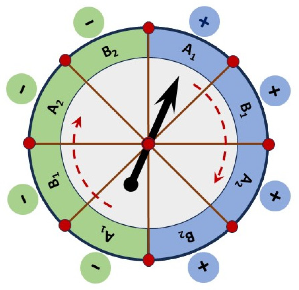
Figure 2.
Correlation patterns for different coincidence windows. (a) Quadruple detection results in global joint distributions with four correlated pairs. (b) In contrast, pairwise detection produces an odd combination of three correlations and one anti-correlation. The underlying record of events is identical for both patterns.
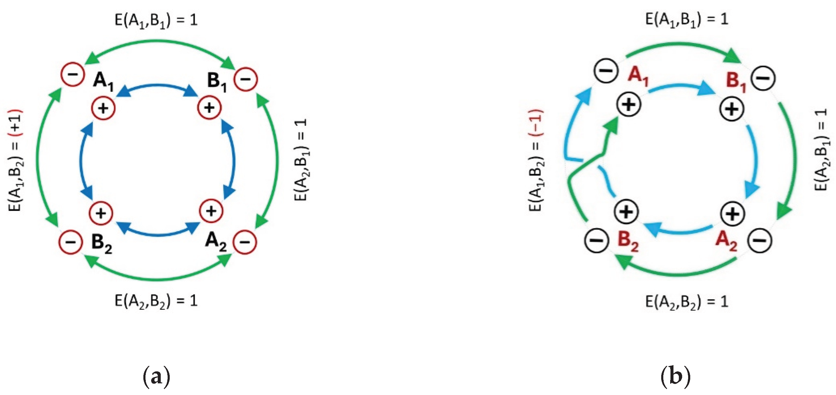
Figure 3.
Visual explanation of the “monogamy” mechanism. (a) Quadruple detection forces pairwise combinations within each batch of four events. Two observables (A1 and B2) must be paired with non-adjacent events. (b) Pairwise detection allows all the events (including A1 and B2) to be paired with the nearest neighbor.
Disclaimer/Publisher’s Note: The statements, opinions and data contained in all publications are solely those of the individual author(s) and contributor(s) and not of MDPI and/or the editor(s). MDPI and/or the editor(s) disclaim responsibility for any injury to people or property resulting from any ideas, methods, instructions or products referred to in the content. |
© 2025 by the authors. Licensee MDPI, Basel, Switzerland. This article is an open access article distributed under the terms and conditions of the Creative Commons Attribution (CC BY) license (http://creativecommons.org/licenses/by/4.0/).
Copyright: This open access article is published under a Creative Commons CC BY 4.0 license, which permit the free download, distribution, and reuse, provided that the author and preprint are cited in any reuse.


