
Submitted:
08 November 2024
Posted:
12 November 2024
You are already at the latest version
Abstract
Modern theoretical physics is built around two myths. The first one is that quantum observables are inseparable from the act of measurement. In some cases, this “observer effect” is supposed to be so strong that some qualities are mutually exclusive. Though, what is the difference between quantum contextuality and classical contextuality? This is where the second myth comes in. Objectively incompatible properties are treated as if they do not exist in classical physics. Instead, only two types of observables are considered: the ones that can occur at the same time as part of a single system, and the ones that are produced by measurement artifacts. As a result, we have a gap between two incomplete theories: a “quantum” theory without objective processes and a “classical” theory without mutually exclusive events. Together, they create the false impression that quantum entanglement is non-local. This is illustrated below with a clockwork mechanism for predetermined sequential properties. The system produces super-quantum Bell violations, as well as the features of quantum monogamy, in ideal experiments without loopholes. A separate illustration, with a classical fluid flow-splitter, is used to explain quantum-like Bell violations with independent and random measurement settings at remote stations. Objective contextuality is the missing piece of the quantum puzzle.
Keywords:
quantum entanglement
; EPR paradox
; Bell’s Theorem
; CHSH inequality
; locality
; realism
; free will
; gedankenexperiment
1. Introduction
Quantum contextuality is widely regarded as a defining feature of microscopic behavior. It means that measurement outcomes do not reflect objective physical properties. Instead, they exhibit qualities that are inseparable from the act of observation. At one extreme, this is interpreted as proof that human intentions create reality. At the other extreme, this is perceived as a technicality, due to the invasive nature of quantum measurements. Yet, there is a clear consensus that quantum observables are “subjective” in this narrow sense. Either “nothing is real” prior to measurement, or “something else is real”, but the values of detected events cannot be described as independently real. The only problem is that this is a baseless opinion. Quantum detectors are inert counters that confirm the proportion of events at various coordinates [1,2,3,4,5]. They have no meaningful impact on the observed distributions as a whole. Indeed, quantum distributions are expected to match classical patterns for large numbers of events, which is known as the Correspondence Principle [6]. For instance, two laser beams can be directed to intersect each other. If these projections are coherent, they can display interference patterns. In one region, the beams overlap with fringes. In other regions, they are separated from each other. This is not something that observers can manipulate with detectors, be it at the classical or the quantum level. If and when decoherence happens, it has nothing to do with the process of observation. In the same vein, it seems problematic that quantum momentum and quantum position are never sharp at the same time. However, quantum experiments do not inspect individual particles for intrinsic qualities. Instead, they count large numbers of events to verify “momentum” distributions or “position” distributions that are predicted with wave-functions. For example, optical projections have sharp momentum spectra in the focal plane of a lens, and sharp position spectra in the image plane (Figure 1). At the quantum level, the same photon counters are moved from one plane to another for detection [7]. There is no “momentum detector” or “position detector” that can change something about these distributions. To sum up, quantum mechanics is supposed to express a new type of behavior with measurement-dependent properties. By implication, quantum entanglement cannot have classical analogues. Yet, as will be shown below, this is pure fiction.
Quantum contextuality is not just a “quantum” problem. It goes hand in hand with distortions in classical statistical analysis. In particular, joint measurements are defined in probability theory as operations to be conducted over a single sample space [8,9]. Physically speaking, this is like measuring different properties of marbles from a single jar. When two correlated systems are measured at a distance, they are supposed to be physically independent from each other. This is akin to observing marbles from two different jars. Therefore, each system must be represented by a different sample space. In this case, joint measurements cannot always express the features of jointly distributed variables. Instead, they produce (for lack of a better concept) coupled distributions [10], with distinctive features. The nuance is that some variables are compatible, like marble properties, with no statistical difference between joint and coupled distributions at the system level. Yet, some variables are incompatible, displaying mutually exclusive values (e.g., optical polarization). In this case, joint distributions are impossible by default. The only way to force joint observations is by sampling incompatible variables from different sample spaces, as it is done in EPR-type settings. This means that each pair of variables becomes coupled in a different virtual space. If lumped together, such couplings cannot always fit in a single sample space, with a global joint distribution. In many cases, this would require intelligent coordination-at-a-distance. Unfortunately, modern physics defines “Local Realism” as the idea that remote measurements always probe a single sample space with jointly distributed random variables. This is why “local” observables are expected to obey Bell-type inequalities [11,12,13]. In other words, the interpretation of correlated behavior is upside down in the case of mutually exclusive variables: objectively local relationships are described as “non-local” and vice versa. The source of this confusion is found in the false dichotomy that defines modern physics. In a nutshell, physical properties are described as if only two alternatives are possible: either they all exist at the same time, in a single context, or they express measurement perturbations. Objectively incompatible classical properties are simply not acknowledged. As a result, the only “allowed” source of Bell violations is to be found in measurement imperfections. If technical loopholes are closed, then “quantum magic” is perceived as the only remaining explanation. In contrast, the concept of objective contextuality eliminates the problem altogether, as will be shown below.
At first sight, the distinction between objective and subjective contextuality may seem misleading in this discussion. Aren’t measurement perturbations also objective processes? Though, it turns out that measurement effects in quantum theory are used in ways that entail “intellectual” side-effects. The problem is that every statistical deviation (relative to the properties of single sample spaces) is automatically interpreted as a result of outcome perturbation. In many cases, physical reasons for such effects are not available and we end up with metaphysical explanations. In the case of non-commuting pairs of variables, one observation is supposed to force an undetected observable to become unsharp [14]. This is supposed to work as if a quantum “knows” which property will be measured, changing its profile accordingly. In the case of spin one-half variables, the same event is supposed to have different values, depending on measurement choices at a distance [15]. It works as if an “Alice” quantum knows which variable is going to be detected by “Bob” with another quantum. In the case of quantum monogamy, the same pair of variables change their coefficient of correlation, based on the number of quanta that are also observed in parallel [16]. This seems to work as if individual quanta know how many events are recorded at the same time, choosing what to display in each case. Officially, such explanations are presented as unavoidable, as if no logical alternatives are possible. In actuality, they are only forced by the decision to treat measurement effects as the exclusive source of physical incompatibility. Hence, they expose the absurdity of this interpretive strategy. If we consider objectively contextual classical properties, it turns out that all of those phenomena can be explained with predetermined outcomes that do not change their values during observation. This is illustrated below with a rotating arrow that points towards different measurement outcomes in sequence, one at a time. Incompatible measurements require different copies of the same system. When two copies are used, Bell violations become possible as a matter of course. If four copies are used, then the rule of pairing is automatically changed. Three pairs of events remain identical, but the fourth pair is coupled “against the grain”. This is sufficient to produce the appearance of “monogamous” correlations. The crucial detail is that individual outcomes are exactly the same in each case, as fixed in advance. The method of coupling alone is responsible for switching one coefficient of correlation, with downstream effects on the Bell index.
To sum up, quantum-like correlations are ordinary classical phenomena. They emerge when incompatible measurements are combined into a single experiment. However, it is not the act of detection that makes these outcomes incompatible. It is the simple fact that some physical properties are mutually exclusive. In other words, there are objective reasons for this, typically described as “hidden variables”. This is why Bell violations are possible with fixed predetermined values, as explained below. Unfortunately, this was not possible to appreciate before, because of the blinding effect of the Copenhagen interpretation, particularly with regard to quantum contextuality. The most influential arguments about Local Realism, including the EPR paradox [17] and Bell’s Theorem [18], were defined by their tacit acceptance of measurement artifacts as the exclusive source of incompatible behavior. To the best of our knowledge, this interpretive problem was not publicly acknowledged before. Nonetheless, the shown solution did not come out of the blue. The true scope of Bell’s Theorem has been questioned for decades, going back at least to 1972 [19,20]. Notable recent contributions include Khrennikov’s study of Bell-type inequalities before Bell [21] and various arguments about statistical compatibility [22]. Another inspiration was the work of Cetto and collaborators on the ontology of the bipartite quantum correlation function [23,24]. The team of De Raedt was also influential in this space for many years with numerous simulations and empirical counterexamples [25,26,27]. Yet, the true number of contributions to this topic is too large to list here. This problem was discussed regularly at conferences, ever since Bell’s argument became popular [20,28,29]. The current name for this objection is the contextuality loophole [30]. Though, upon closer inspection, the word “loophole” is misleading in this case. It seems to imply that Bell’s Theorem is correct about classical mechanics, and that special experimental exceptions are needed to achieve violations. Indeed, contextual objections to quantum non-locality are often lumped under the umbrella of the detection loophole for Bell experiments [31]. In rare cases when contextuality is discussed as a classical process, the general tone is that special assumptions are still needed, in order to explain how it works. In short, objectively contextual solutions were not given proper consideration. Instead, they were constrained by misperceptions about measurement effects and statistical anomalies. As a result, there was this strange puzzle: the math entailed local solutions, but every physical explanation seemed to beg for non-locality. In order to finally move forward, the solution is to acknowledge the “unthinkable” facts. Quantum observables are neither created nor modified by the act of detection. Perturbations are technically possible, but they are irrelevant for the fundamental aspects of this problem. Some physical properties are incompatible by default, and they can happen at any level of analysis, be it quantum or classical. As will be shown below, objective contextuality is sufficient to explain “quantum” and even “super-quantum” correlations with classical processes.
2. CHSH Violations with Sequential Properties
Classical physics is associated with a deterministic model of the Universe, in which conserved amounts of matter display mechanical interactions like clockwork. This would suggest that all the fundamental properties are also conserved and permanent. It seems intuitive that all of these qualities should be compatible with each other, meaning that they must all exist at the same time. However, the main function of clocks is to reflect the passage of time. Ergo, they must express mutually exclusive properties. If the arrow of an analogue clock points to 1 o’clock, then it is not pointing to 2 o’clock. If it is pointing towards 6 o’clock then it cannot be pointing towards 7 o-clock, and so on. Thus, a classical description of our Universe would be incomplete without objectively contextual properties. The question is: how can we obtain coincidences and correlations between mutually exclusive events? Like the sound of one hand clapping, such phenomena are impossible as part of a single system. At first sight, we could create two copies of the same system and look at the coincidences between them. Yet even here we have a complication. If the two systems are perfectly identical, then they always express the same property at the same time, and coincidences between incompatible events are impossible. On the other hand, if one of the two systems is modified, to enable incompatible observations, then we are no longer detecting coincidences between identical processes. Upon further consideration, the solution is to change the definition of simultaneity. Instead of recording pairs of instantaneous events, we can choose to consider pairs of events in an extended window of coincidence. In the case of clockwork systems, it is possible to isolate consecutive observables in pairs, if the window of coincidence is wide enough to include two events, but not wide enough to include three or more. Remarkably, it is not even necessary to use two copies of the same system in this case, as both measurements can be achieved at the same location. Yet, from a formal point of view, we should still treat this example as a coupling between two independent (but correlated) systems. After all, we are detecting properties that cannot be jointly distributed in a single sample space. The manifestation of two properties in pairs is a forced phenomenon, contradicting the actual structure of the underlying system. In other words, an extended window of coincidence corresponds to a coupling between two mutually exclusive instantaneous events, as if they are probed in two different sample spaces.
A chain of pairwise connections on a clockface must close back on itself. This is convenient, because a Bell-type experiment is also a closed chain of pairwise measurements, such that any single variable is measured in coincidence with two others [32]. So, let us attempt to replicate a CHSH experiment [33] with staggered properties in a “clockwork” classical system (Figure 2). Consider a large (classical) object in the shape of an arrow, rotating above a table with printed markers. Any imaginary axis through the center of the table is crossed by the arrow twice per full rotation. Accordingly, it is possible to assign binary values to opposite ends of each axis, such as “+” for North and “−” for South, or “+” for East and “−” for West (etc.), as shown in Figure 2a. The “outcomes” for each axial variable must exhibit 50-50 distributions, as long as the arrow is moving continuously. The CHSH protocol requires 4 binary variables. Therefore, it is possible to replicate a Bell setting with four suitably arranged axes. For clarity, the surface of the underlying table can be divided into 8 sectors, as shown in Figure 2b. A1 and A2 values are interlaced with B1 and B2 values, in order to enable the pairwise detection of all the necessary combinations for a Bell test. If the arrow is forced to rotate at a fixed rate, by means of an actuator, it passes over each sector, one at a time. If the arrow is in the state of hovering over sector “A1+”, then we can describe this observation as a “conditional real outcome”. The same rule applies to all the other sectors, in sequence, resulting in a simple toy model with contextual classical properties. Anyone of the 8 outcomes has an equal probability of manifestation, which means that the distribution of opposite values for each variable, conditional on it being selected for detection, is 50-50.
A well-known feature of quantum entanglement is that Bell violations happen for pairwise measurements (and only for pairwise measurements [16]). Such patterns are not possible for systems with jointly distributed variables. For example, as shown in Figure 3a, maximally correlated simultaneous properties exist in homogeneous quadruplets. Objectively, all the four observables have “+” values, or all of them have “−” values, depending on which iteration is chosen. Hence, pairwise detections cannot do more than to sample this underlying pattern. The outcome is a set of Kolmogorov -compatible set of coefficients of correlations. The CHSH inequality for this case is:
Given that all the pairs are maximally correlated in the described example, and that all the expectation values are equal to 1, we get:
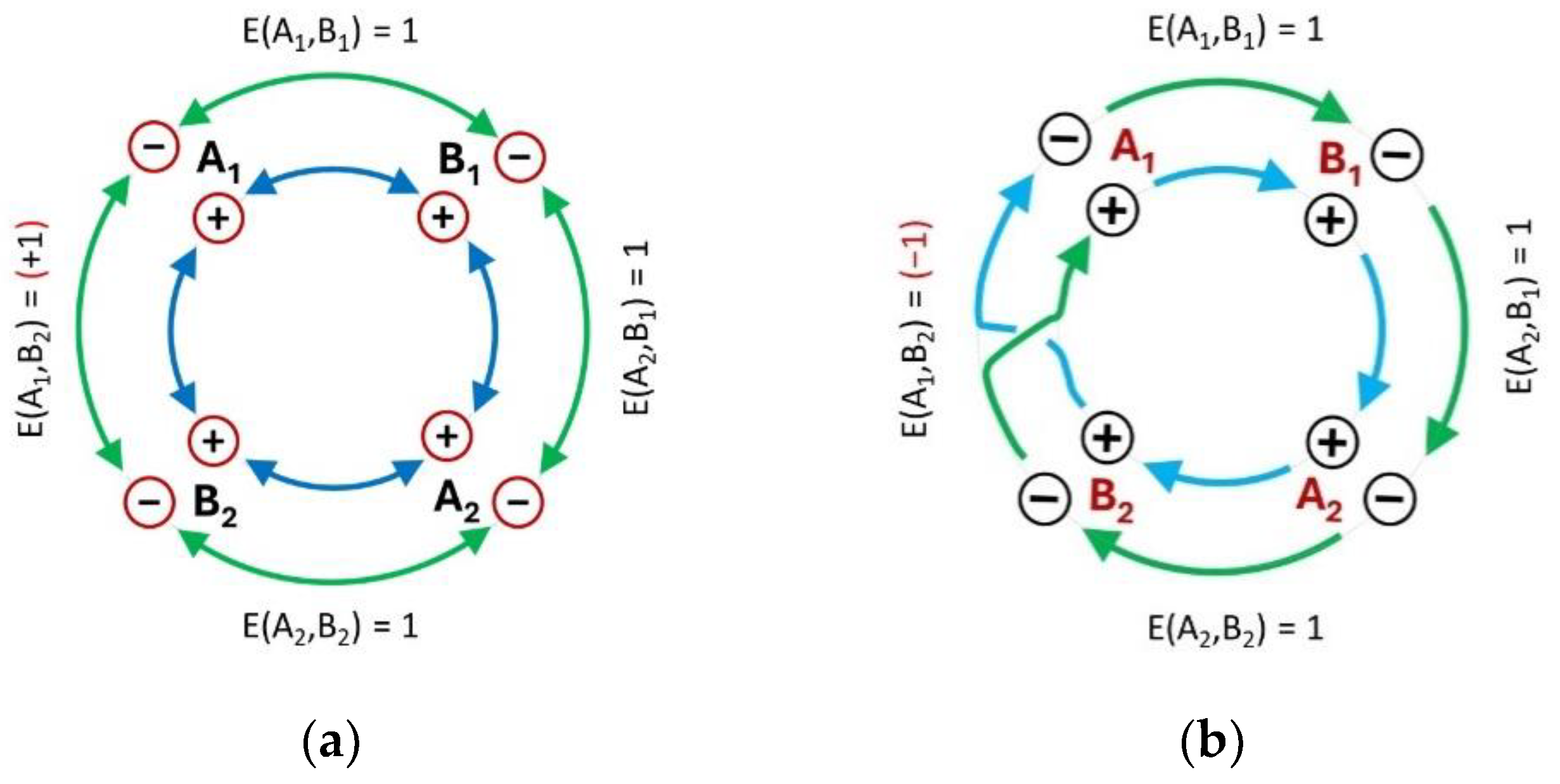
In contrast, sequential properties are not limited in the same way. Instead, a full cycle includes all the 8 possible observations in a closed chain of pairs, resulting in a Möbius-strip pattern, as shown in Figure 3b. The net effect is a combination of statistically incompatible coefficients. Three pairs of observables can only coincide with (+, +) or (−, −) outcomes, making them maximally correlated. In contrast, one pair is only able to coincide with (+, −) or (−, +) outcomes, due to the double crossover between the inner and the outer loops of the Möbius strip. This makes it maximally anti-correlated. When plugging these values into the CHSH expression, we get:
Such a mixture of pairwise combinations is logically impossible for objectively simultaneous properties (). Nonetheless, it emerges naturally in a system with predetermined sequential properties (. We have a classical mechanism that operates like a clock, whether or not it is observed. All the values are printed on the table and cannot change just because the arrow is passing over them, or because a person is looking at them. Each transient outcome is flanked by two different sectors on the table. So, pairwise consistency is maintained throughout, meaning that distributions (A1, B1) and (B1, A2) always agree about the values of B1, while (B1, A2) and (A2, B2) always agree about the values of A2, etc. This satisfies the requirement that Alice’s (or Bob’s) event is always the same, no matter what Bob (or Alice) is doing. In short, the mechanism is fully transparent and the reason for the final outcome is obvious. Maximal Bell violations are not only possible in coupled measurements, but they also happen to be very common. Any system with spinning objects can produce them.
This is a good place to review the question: why did people believe in quantum nonlocality? The answer is that Bell violations did not seem possible with predetermined values. In all the debates on quantum behavior, the concept of Realism is defined to include only simultaneous properties, as shown in Figure 3a. (Any manifestation of incompatible behavior is automatically presented as a measurement artifact). Indeed, in this case, Bell violations are logically ruled out. The only way to achieve incompatible coefficients is by perturbing the input values in incompatible ways. For example, the same Alice measurement of A1 must yield a “+” outcome if Bob measures B1 and a “−” outcome if Bob measures B2. Such coefficients are not classically possible (either physically, or in the sample space representation), and the only way to achieve them is with measurement perturbations. This is why there were so many discussions about “fair sampling” with regard to Bell experiments. This is also the motivation for developing new technologies for “loophole-free” Bell experiments. Notwithstanding, it turns out that Bell violations are quite natural for mutually exclusive objective properties. This is particularly important, given that quantum theory predicts Bell violations for non-commuting variables, and only for non-commuting variables.
Figure 3.
Coincidence patterns for simultaneous vs sequential properties. Jointly distributed variables can only have compatible coefficients of correlation. This rule does not extend to mutually exclusive (but still objective) properties. (a) Simultaneous realism entails that all the variables express their values at the same time, for each object. In a population with maximal correlations, each object is either represented by the green circle, or the blue circle. Pairwise observations sample this pattern and cannot violate the CHSH inequality. (b) Sequential realism enables the pairwise detection of two observables at a time, with no regard for the state of other properties. The same Möbius-strip pattern is replayed over and over. Both loops must be traversed in full before returning to the same starting point. Maximal CHSH violations emerge, as explained in the text.
Another surprise of this illustration is the ability to produce maximal Bell violations. The prior state of “textbook” knowledge was that Bell violations were impossible in classical mechanics. Quantum theory was known to predict such phenomena, but only up to the so-called Tsirelson Bound [34]. Yet, correlations beyond this limit were described as “super-quantum”, and they were presumed to entail new physics [35,36]. (Perhaps, parallel Universes? [37,38]) An interesting exception is the so-called “coincidence loophole”, wherein maximal Bell violations are possible with jointly distributed properties that are inaccurately paired [39,40]. In other words, we have simultaneous observables that cannot violate the CHSH inequality objectively, but events from the wrong coincidence windows of Alice and Bob can be mixed up in just the right pattern for a maximal Bell violation. In this case, we have a distortion of the underlying reality, due to methodological errors. In contrast, what was shown above is a natural manifestation. Mutually exclusive events cannot be simultaneous. Therefore, they cannot be jointly distributed. Even when they are coupled in ways that obey the CHSH inequality, they still exhibit artifacts that do not emerge from any single sample space. More importantly, maximal Bell violations are achieved here by detecting events from the adequate coincidence window. Ergo, this is not a loophole that needs to be closed. Nonetheless, there is a subtle aspect of this demonstration that needs to be explained in greater detail.
If we consider Alice-Bob experiments with simultaneous properties, then Bell violations are not possible in ideal conditions. Yet, rapid sequences of events can lead to spurious coincidences, such that Alice’s measurement #1 is accidentally paired with Bob’s measurement #2 (to give just one example). In this case, Bell violations can happen, but only in suitable patterns of detection. A good way to close this loophole is by enforcing random measurement settings, independently for Alice and Bob. However, there is no such loophole in the example discussed above. For instance, if two copies of the same arrow mechanism are used for an EPR-type experiment, the two stations need to maintain their correlation for a fair test. A complete measurement of all the events will produce Bell violations. A random measurement scheme (like in the game “Wheel-of-fortune”) will have the same effect. Yet, sudden interventions to stop the rotation (independently for Alice and Bob) would break the correlation between the two systems. On the one hand, independent settings are fatal for the experiment, just like in the case of the “coincidence loophole”. On the other hand, the physical meaning of this effect is different. A test of locality cannot be achieved by destroying the basic features of the targeted mechanism. Instead, sequential properties must be replaced with alternative mutually exclusive properties. In this case, spontaneous transformations are integral to the underlying ontology and Bell violations cannot be foiled by independent changes to the experimental set-up. This is described and explained in the next chapter.
3. CHSH Violations with Alternative Properties
Quantum distributions are often dressed in metaphysical jargon, but they are known to display the same relationships as their classical counterparts. For example, a stream of polarized photons can be split at arbitrary angles by a polarizing beam-splitter (PBS). If the PBS fast axis is aligned at 45° to the input plane of polarization, then 50% of the photons are transmitted and 50% are reflected. Yet, an interaction at 22.5° will transmit 85% of the photons (with 15% reflected). This means that two deflections of 22.5° will produce an output beam with diagonal polarization, while retaining about 72% of the input number of photons. It is not possible to reconcile two polarization deflections at 22.5° with one deflection at 45°, even though the output polarization is the same. Yet, this is the same pattern that emerges in the interaction of classical laser beams with PBS devices [41,42]. In both cases we have group-level properties that cannot be explained as pre-existing at the input. We are dealing with mutually exclusive observables. Nonetheless, individual outcomes can have pre-determined conditional values, because they are caused by deterministic intervening processes.
Let us consider a quintessential classical entity – the billiard ball. When such an object is rolling on a rigid flat table, it has a well-defined velocity. It also has a well-defined momentum (p=mv) and a corresponding amount of kinetic energy (Ek=mv2/2) at any coordinate on its trajectory. This means that one and the same classical property (i.e., velocity) has two different implications. One of them can exhibit linear transformations, but the other one is non-linear. For example, if a billiard ball collides with another ball at an angle, it transfers part of its momentum and is deflected into a new direction. Assuming equal mass for the two balls, the new momentum magnitude is determined by the cosine of the angle between the input and output velocity vectors (pout=cos(θ)pin). Yet, the retained amount of kinetic energy is determined by the cosine squared of the same angle (Eout=cos2(θ)Ein). So, if a ball is deflected at 45° in a collision, it retains 50% of its input kinetic energy (Figure 4a). Yet, two consecutive deflections at 22.5° result in the same output direction with 72% of the input amount of energy (Figure 4b). This is the same pattern that is predicted by Malus’ Law for optical polarization redistribution. We measure beam power at the macroscopic level, and we count photons at the microscopic level, but the observable system-level behavior is the same. If we interpret these phenomena in terms of objective interactions with energy redistribution, rather than as measurement artifacts, then we have no need for speculations about “quantum magic”.
The question is: can we produce Bell violations with billiard balls? On the one hand, we have non-linear transformations that produce incompatible properties. So, it should be possible to find at least one Bell-type inequality that is violated in this case, compared to a system with compatible properties. On the other hand, it is not possible to achieve CHSH violations with such systems, because there are two complications. The first problem is that energy redistribution is a systemic property, and a single ball is “the system” in this case. It is not possible to break the kinetic energy of a billiard ball into statistical increments. Another complication is that non-linear effects have a variable angular density in this case. At some angles, the rate of change is disproportionately low compared to linear transformations. At other angles, it is disproportionately high. Yet, CHSH experiments require a wide net angular span, and these effects average out at such a scale, as if converging to a linear baseline. On closer inspection, however, both of these concerns can be allayed by a single solution. Quantum theory does not predict Bell violations for sharp properties. The only way to achieve them is with “undefined” beams, where multiple virtual components are superposed and act at the same time. We have such patterns of behavior in classical fluids, where the path of individual particles is inseparable from the collective effect of other particles. As a result, we can replicate Stern-Gerlach quantum statistics with a classical flow-splitter mechanism.
Consider a T-junction between three pipes, as depicted in Figure 5a. Fluid comes down through the vertical pipe, and then it is split 50-50 in opposite directions along the horizontal pipes. The key feature is that the junction is flexible, making it possible to rotate the horizontal section at will. At the input, any molecule in the fluid has an equal probability of flowing either to the left or to the right. Yet, this is a classical system, and we do not have “ontological uncertainty”. Perfect knowledge would show that either outcome is uniquely determined by the physical interactions along the complete trajectory from the input to the output (similar to a coin toss). Theoretically speaking, it is possible to describe two identical copies of such a system (and even to simulate them on a computer), such that every molecule of fluid in the “Alice” copy has an identical partner with an identical trajectory in the “Bob” copy. Accordingly, if one molecule ends up going to the right in the Alice device, then its twin will also emerge in the same direction in Bob’s device 100% of the trials.
Nonetheless, the molecules do not have ballistic trajectories. Their motion as individuals is inseparable from the motion of the fluid as a whole. Therefore, we can analyze the fluid as a macroscopic entity that experiences energy redistribution, just like a billiard ball in a collision. The difference is that we are not deflecting the fluid from its original direction, but rather redistributing it in the transverse plane. The equivalent rule for Malus’ Law (Eout=cos2(θ)Ein) becomes in this case:
In other words, the input amount of energy is always split 50-50, either for setting 1 or for setting 2 in the x-y plane. However, the output in one channel, treated in isolation, contains a proportion that would have been the same in the first orientation, and a supplementary proportion from the other channel. The value of this proportion is determined by the cosine squared of half the angle θ between the two settings. For example, if the fluid is split 50-50 along an arbitrary 0°-180° axis in the x-y plane (Figure 5a), we can assume that this is not an accident, and that half of the input fluid had an inertial propensity to end up in the 0° direction. We can then ask: how much of this fluid (or, what proportion of molecules) would have still emerged in the same channel, if the pipe was rotated by angle θ in the x-y plane? In keeping with the known patterns of energy redistribution (as described above), we should expect this proportion to be determined by the cosine squared of half the angle of deflection. For example, 100% of the molecules should be the same if the difference is 0°, and 85% should be the same if the pipe is rotated by 45° (with the remaining 15% coming from the opposite channel). Similarly, 50% of the fluid molecules should be the same at 90° rotation, and 0% should be the same at 180°. This conditional pattern is rotationally invariant, since it holds for any pair of alternative orientations of the output pipes. In short, fluid molecules in a flexible T-junction display the same type of behavior as a beam of silver ions in a Stern-Gerlach device.
A quantum CHSH experiment can be replicated with a classical flow-splitter as follows. Two identical systems are simulated by independent computers, one for Alice and one for Bob. The fluid flows continuously, but single molecules of some traceable dye are injected one at a time. The goal is to detect these dye molecules one by one, in large numbers, for statistical analysis. Each tracer molecule for Alice has an identical twin in Bob’s device. The die molecules are carried by the fluid in identical ways, and always display identical behavior from the input to the flexible splitter. Notably, the trajectories of dye molecules are determined by the properties of their surrounding volumes of fluid. For example, if 50% of the fluid molecules are the same in two output settings, then the probability of one die molecule to express the same outcome in both cases is also 50%. The horizontal pipe is randomly and independently switched between 0° and 90° for Alice, and between 45° and 135° for Bob. (These settings are known to produce the highest possible Bell violation in quantum experiments). As a result, four types of pairwise combinations are possible, as shown in Figure 5b: A1B1, B1A2, A2B2 and A1B2. Three of these settings are separated by 45°, meaning that 85% of the expected outcomes are the same for Alice and Bob, while 15% are different. The approximate coefficient of correlation in this case is 0.7. Though, a more accurate formula is:
The remaining combination has an angular difference of 135°. Hence, the coefficient of correlation is:
If these expectation values are plugged into the CHSH formula (equation (1) in the previous chapter), then we get the following result:
To sum up, Bell violations up to (but not exceeding) the well-known Tsirelson Bound are natural in classical systems with mutually exclusive alternative transformations. Though unrecognized, the conditions for such effects are omnipresent in the modern world, since water supply lines with T-junctions are no less common than analogue clocks. Moreover, the fundamental reason for this behavior is energy redistribution, which is a basic classical process. Another useful conclusion is that random measurement choices cannot be used to validate nonlocality for quantum entanglement. Incompatible properties can be sequential (in which case they produce maximal Bell violations, but their order is essential), or they can emerge from alternative arbitrary transformations (in which case they can be produced at will, but with limited Bell violations). Loopholes can only be closed if they exist. As it is known, simultaneous properties cannot be inconsistent, unless there are measurement imperfections. In some cases, detection problems can be fixed with arbitrary choice strategies for the settings of Alice and Bob. Yet, measurement imperfections are not the only source of incompatible behavior. It was a mistake to look for them in the case of quantum measurements, where the “observer effect” was an imagined phenomenon.
4. “Monogamous” Correlations with Predetermined Events
The concept of joint distribution is elementary in probability theory, but it became surprisingly confusing in the context of quantum mechanics. Physical objects have numerous permanent properties. This means that every object displays simultaneous values for each corresponding variable. As a result, all of these variables can be represented in a sample space as jointly distributed. Conversely, when such a space is being sampled as part of a simulated observation, the law of large numbers entails that output data must also be jointly distributed. In other words, it is possible to construct a consistent one-to-one mapping between all the elements of each set of measurement outcomes, even if different variables are not sampled at the same time. Thus, a global joint distribution in the data is a faithful reflection of an objective joint distribution in a given physical system (or its abstract representation), assuming perfect methodology. The nuance is that the reverse is not necessarily true. When two or more measurements are performed at the same time, output data is jointly distributed by default, since every iteration produces coupled detections [10]. Consequently, it is possible to measure two unrelated systems or more, generating joint distributions in the data without any factual connection to some objective joint distribution of physical traits. The explanation is that we are studying relationships endemic to the product of two sample spaces (or more), as opposed to relationships between the variables of a single space. Unfortunately, this aspect was ignored in the context of quantum mechanics. Instead, the Hilbert space is often perceived as a standalone “non-classical sample space” [14]. Hence, quantum behavior was often interpreted as if joint distributions in the data were automatically indicative of a joint distribution in Nature. This created a lot of confusion for the analysis of non-commuting variables. If physical properties are mutually exclusive, how can they be jointly measured? Or, if the data shows joint distributions for joint measurements, how can we describe these variables as non-commuting? The simple answer is that physical properties do not need to exist at the same time in order to allow for coincident observations. This can be seen by reviewing Figure 1 above. In other words, patterns of joint detection can inform us about patterns of transformation from one context to the next, rather than about rates of objective coincidence in single contexts. Therefore, it does not follow that real qualities change their nature from sequential to simultaneous, just because they are studied with joint measurements.
This insight is particularly relevant for the analysis of quantum monogamy. In modern physics, entanglement is often described as a “telepathic” connection between remote quanta. Moreover, Bell violations are interpreted as markers for such connections. Any failure to produce incompatible coefficients is automatically described as a loss of connection (i.e., loss of entanglement). It turns out, however, that quanta can only exhibit CHSH violations when measured in pairs. If three or more entangled quanta are selected for measurement, then no violations are possible. This is the essence of the so-called “monogamy of quantum entanglement” [16,43,44,45]. If quanta have the magical power to communicate instantaneously across the Universe, why can they not use the same ability to generate Bell violations in larger clusters? The apparent implication is that quantum entanglement has ethical standards, such that pairs of quanta remain “monogamous” to each other, or they can also be “promiscuous”, but they only express their “love” in pairs (as if they obey a “no orgy” principle). Unfortunately, these tongue-in-cheek interpretations obscure the true mystery of this phenomenon. When joint measurements are performed, the data stream is necessarily coupled, producing pseudo-joint distributions. If two variables are measured at the same time, then the two of them express joint distributions by default (even if corresponding observables are mutually exclusive). Yet, different pairs of observations can still be incompatible with each other. In contrast, if all the variables of a system are measured at the same time, then global joint distributions are produced in the data. Accordingly, it is technically impossible to achieve incompatible coefficients of correlation with 4-quantum entanglement in a CHSH protocol. Four events at a time are produced in each iteration, as if the four qualities exist in a single context at the same time. Therefore, it is not “weird” per se that Bell-type inequalities are obeyed. The challenge is to explain what happens to entanglement.
At first sight, this phenomenon is a direct confirmation of “quantum weirdness”. In one context, only two quanta are detected at a time and Bell violations are possible. In another context, four quanta are detected at a time and Bell violations are impossible. Yet, this means that one and the same pair of quanta exhibits radically different patterns of coincidence, simply because other quanta are measured or not measured at a distance. This conclusion must hold even for ideal experiments, without bias, event loss, or technical challenges. So, how is it possible for two variables to have opposite coefficients of correlation in the same measurement? How do these two quanta “know” that other quanta are measured in parallel or not? (And, more importantly, why do they “care”?) It seems impossible to explain this phenomenon with predetermined event outcomes, since the final result depends on external non-local factors. Nonetheless, a straightforward solution is available. As shown above, Bell violations do not require all the coefficients to flip values, compared to the example with compatible properties. Indeed, such behavior would have null effects on the final sum of coefficients, as multiple perturbations would cancel out each other’s effect. A maximal CHSH violation requires three coefficients to remain strongly correlated, while only one of them is anti-correlated. Similarly, only one coefficient of correlation needs to become different in a four-quantum detection scheme, in order to make Bell violations impossible. Yet, just like in the case of Bell violations, this effect does not require the measurement outcomes to be altered in any way. Instead, three coefficients of correlations can remain the same, while the fourth one is forced to change polarity by the protocol of detection.
The key to this mystery is to recall that mutually exclusive properties cannot be real at the same time, as part of a single system. When we force the simultaneous observation of such qualities, either in groups of two or in groups of four, we are always creating pseudo-joint distributions. Thus, a global joint distribution in the four-quantum scheme does not reveal a “return” to some objective classical state. This apparent “loss of entanglement” is just another artifact of the decision to combine incompatible properties into a single experiment. Given that joint distributions cannot exist objectively, both patterns – with and without Bell violations – represent distortions of the objective relationships between such properties. Instead, the coefficients of correlation reveal the rules that connect different sequential contexts to each other. The mechanism is shown in Figure 6.
Pairwise detection requires a relatively narrow window of coincidence, such that two events at the most are collected in each trial. This means that binary variables B2 and A1 are always going to exhibit anti-correlations, since their adjacent values are on opposite halves of the table in Figure 2. At the same time, the remaining three pairs are adjacent on the positive or the negative side of the table, resulting in strong correlations (Figure 6a). A blind detection scheme, in deal conditions, must produce maximal Bell violations, as shown in one of the preceding chapters. In contrast, a four-event detection scheme requires a much wider window of coincidence for the same clockwork system. This means that the objective sequence of events is now artificially broken into chunks of four values, counted as a pseudo-simultaneous group. All of a sudden, the instantaneous value of B2 can no longer be paired with the adjacent value of A1. Instead, it is forced to be counted in pseudo-coincidence with the remote and opposite value of the same observable (Figure 6b). To sum up, a set of fixed pre-existing values are detected without measurement artifacts in both protocols. Instead, the method of data processing is different in each case, such that three coefficients of correlation remain unchanged, and the last one is flipped to its opposite value.
We see again that EPR-type phenomena are distorted by ungrounded interpretations, at every level of complexity. If we assume that measurement outcomes are inseparable from the act of observation, and if we further deny the existence of objectively incompatible properties, then quantum phenomena appear to emerge from measurement artifacts. As a result, we get paradoxes. Yet, more often than not, contradictions are due to mistaken assumptions, rather than to the existence of super-physical forces. This case is not an exception. If we acknowledge the reality of objectively incompatible physical properties, the same phenomena can be explained with simple mechanisms and predetermined measurement outcomes, including quantum monogamy.
5. Two Kinds of Local Realism
Quantum behavior is often described as “irreducibly non-classical”. Moreover, this is not supposed to be a matter of opinion. Bell’s theorem is a well-vetted argument, with rigorously defined ontological assumptions. If a Bell-type inequality is violated by adequate experiments, then one of three conditions must be false: either “Realism”, or “Locality”, or “Free Will”. Notwithstanding, the classical examples shown above can satisfy all of the three ontological conditions (Realism, Locality and Free Will) while contradicting all of the three mathematical concepts with the same name. (In this article, quotation marks distinguish the labels of mathematical constructs from the words that denote ontological referents with identical titles). Consequently, the problem is not that we have “quantum magic”. The problem is that wide ontological concepts have been improperly mapped to excessively narrow mathematical conditions. This is why quantum correlations were misinterpreted.
5.1. Realism vs “Realism”
In the context of correlation analysis, the notion of “Realism” is defined as the principle that pairwise measurements can be described by two families of random variables:
for one measurement site with local setting , and
for another measurement site with local setting .
Yet, this apparent simplicity of notation conceals a complex theoretical construct, including a sample space with hidden variables and a system of rules for mapping the elements of this space to expected measurement outcomes [31]. The most important feature of this definition of “Realism” is that measurement outcomes are amenable to analysis with classical (Kolmogorov) probability theory. In other words, we assume a Universe in which all the detectable quantities correspond to objective properties that are well defined at the same time, as part of a single system. This is why the corresponding variables are expected to be jointly distributed [11,12,13].
Some physicists questioned this definition of “Realism” on the grounds that Bell’s Theorem cannot be derived from it. See, for example, the discussions in [29] and [46], and references therein. In other words, it is theoretically possible to achieve Bell violations with predetermined values, given two random variables. However, such solutions required more than one sample space and were largely perceived as non-classical. The mainstream assumption was that multiple sample spaces are required exclusively for the analysis measurement artifacts, and coordination between such systems would have required non-locality.
Contradiction #1: According to this definition of “Realism”, an objective “clockwork” Universe must only include permanent unconditional properties. Yet, as shown above, the most useful feature of a clock is the ability to display conditional properties one at a time. (It must show the time of the day). Just because some properties are mutually exclusive, it does not follow that the Universe is less real. Indeed, the toy models presented above provided transparent mechanisms for Bell violations with pre-determined measurement outcomes. The Realism of these systems is unquestionable, yet the observed type of behavior cannot emerge from a single sample space with jointly distributed variables. Ergo, the mathematical definition of “Realism” does not convey the full ontological meaning of Realism, since it only includes compatible properties [21].
5.2. Locality vs “Locality”
John Bell described the concept of Locality, in plain language, as the requirement “that the result of a measurement on one system be unaffected by operations on a distant system” [18]. This means that every individual outcome should have the same value, no matter which measurement is performed at another site. Another name for this condition is “pairwise consistency”, as mentioned above. Yet, the mathematical definition of “Locality” in Bell’s argument is formulated in terms of average probabilities. In other words, we expect to have “Locality” when the following condition is satisfied (using Bell’s notation):
If the joint probability of two variables is factorizable, by virtue of hidden variables, then they correspond to “Local” observables. This definition seems very intuitive, as long as we are dealing with jointly distributed variables [11]. In this case, it is correct that conditional statistical separability entails pairwise consistency. Nonetheless, the reverse relationship does not hold with necessity. It is possible to have physical independence without statistical separability, particularly when dealing with mutually exclusive observables. As shown above, local properties do not have to be simultaneous. Sometimes they manifest one at a time, alternatively or in sequence. When joint observables are statistically “entangled” as part of a single system, it is not possible to use separability as a marker for influences between remote systems.
Contradiction #2: The Möbius pattern, presented above, displays maximal Bell violations. Accordingly, it contradicts the separability condition, associated with Bell “Locality”. Yet, all the combinations emerge from a clockwork mechanism, as part of a single system. The outcomes are printed on the table in advance and do not change as a result of observation. Moreover, any Alice outcome is naturally paired with both possible Bob outcomes, and vice versa, satisfying the requirement of pairwise consistency with predetermined measurement outcomes. In short, a formal contradiction with “Locality”, as mathematically defined, does not correspond to an ontological violation of Locality.
5.3. Free Will vs “Free Will”
The “Free Will” condition was originally discussed by Bell, as a requirement for unconstrained measurement choices in real experiments. The formal definition was clarified by CHSH in their notorious paper: “we assume that the normalized distribution ρ(λ) characterizing the ensemble is independent of (adjustable parameters) a and b” [33]. The well-known concern here is that a “Local Realist” model, can produce Bell violations if the so-called “detection loophole” is not closed [31,40]. In particular, observable statistics may produce a distortion of the underlying reality if measurement settings are correlated with the hidden parameter λ. This is why Alice and Bob are required to choose their settings independently from each other in loophole-free experiments, for example by employing separate random number generators. Nonetheless, this is more than a technical loophole, given the possibility to invoke “super-deterministic” [47,48,49] or “retro-causal” [50,51] mechanisms for observable correlations between hidden variables and measurement settings. In other words, it is theoretically possible to have random measurement settings, without closing out this “loophole”. Moreover, the plausibility of such explanations is currently accepted as a matter of personal preference, given that other quantum interpretations (such as “many-worlds” and “nonlocality”) are no less strange.
To understand this problem better, consider a Bell-type experiment where Alice can choose to detect one of two observables (A1 or A2), while Bob must always detect two at the same time (B1 and B2). Furthermore, suppose that Bob’s measurement outcomes are always different if Alice chooses A1, and always identical if Alice chooses A2. In other words, we have two incompatible profiles for hidden variables, working in a measurement-dependent basis. There is a clear correlation between Alice’s choice of settings and the underlying rules of coincidence for Bob. Yet, how is it possible for such coordination to emerge, if Alice and Bob are far from each other? One possibility is that observers are actively conspiring together, or else there is some other source of bias in the experimental scheme. This is the loophole that “free” measurement settings are supposed to close. Nonetheless, this concern is only warranted for systems with jointly distributed variables, where variations in hidden variable density are produced exclusively by measurement artifacts. There is no such correspondence in the case of objectively conditional observables.
Contradiction #3: As shown in Figure 2b, A1 outcomes are always flanked by opposite values for B1 and B2, while A2 outcomes are always flanked by identical values for B1 and B2. Mathematically, we have a correlation between two measurement choices and two profiles of “ρ(λ)”, as described in the previous paragraph. Yet, from a physical point of view, we have just one underlying process – an arrow that is rotating continuously. It is not the choice to measure A1 (or A2) that changes the rules of coincidence. It is the other way around: objective processes limit the observation of A1 (or A2) in correlation with different patterns of coincidence for the B1 and B2 observables, as part of a single physical system. (A similar argument was previously made by Geurdes [52]). This is a distinguishing feature of objective contextuality. As seen above, the arrow model is clearly displaying pairwise consistency for A and B outcomes. Alice is perfectly free to choose between A1 and A2, and Bob is perfectly free to choose between B1 and B2, without any impact on the final coefficients of correlation. If non-invasive measurements are replaced with invasive perturbations of this system, then the pattern of correlation can be destroyed, but this becomes a distortion of the underlying reality. As shown above with the flow-splitter model, random transformations cannot prevent Bell violations for alternative properties. Preparatory interventions are faithful to the structure of the tested system in the latter case, even though the underlying mechanism is less obvious than in the arrow model with a Möbius-strip pattern. In short, a contradiction with the “Free Will” condition, as formally defined, does not entail a contradiction with ontological Free Will, even in classical systems.
To sum up, it is possible to contradict all the three criteria for “Local Realism”, as mathematically defined, while observing a system that is obviously Local and Real from an ontological point of view. This would not have been possible, if current tools for testing the nature of reality were adequate. On closer inspection, all the three conditions have the same shortcoming: they only hold for jointly distributed variables. Accordingly, it is not enough for Bell’s theorem to be formally precise. It is not enough for the quantum experiments to be rigorous and loophole-free. Correct interpretations depend on the accurate labeling of relevant mathematical expressions. In this case, the starting assumptions for analysis were incorrect. Therefore, the argument for non-locality was technically valid but the final conclusion was unsound.
6. Discussion
Classical mechanics was famously unable to cope with the discovery of quantum phenomena. Bohr and his followers described the problem as fatal. They argued that old models of Reality should be abandoned entirely. Yet, Einstein and his followers disagreed. They called for more patience in the search for final answers. The pinnacle of this debate is a pair of notorious papers with the same title: “Can Quantum-Mechanical Description of Physical Reality Be Considered Complete?” [17,53]. In hindsight, a better strategy might have been to ask whether classical theory was formally complete. It is in the nature of physical entities to experience transformations. Therefore, single systems require multiple quantitative representations, as these changes manifest in sequence. Unfortunately, the instruments for studying such transformations, and especially their statistical aspects, were not fully developed (or, at least, not widely adopted) at the turn of the 20th century. Had there been an established practice for dealing with objective contextuality, it would not have been necessary to propose (let alone to accept) metaphysical models with subjective contextuality. Paradoxically, quantum theory is more “complete” than classical theory in this formal sense, but it was an interpretive disaster. The real problem was the entrenched tendency to explain physical transformations with measurement artifacts, especially in cases where no such artifacts were possible. In short, modern physics is incomplete in a strikingly obvious way: it does not acknowledge objective system-level transformations. As a result, it has inadequate tools for studying the mutually exclusive properties of fluid systems.
An interesting aspect of this topic is the rapid success of metaphysical interpretations, while classical-style approaches had to justify their existence. Quantum theory was developed to analyze measurement outcomes, rather than physical processes that can be observed. By interpreting the formalism literally, physicists ended up attributing a special status to the concept of measurement. As a result, it became unthinkable to even question the existence of detection artifacts in quantum mechanics. Yet, looking at this problem with fresh eyes, it turns out that the observer effect was a red herring. It motivated perennial debates: is it the human intentions or the measurement devices that distort the unmeasured reality? Instead, the question to ask was: do such perturbations exist in the first place? Quantum theory was explicitly developed with the Correspondence Principle in mind. In other words, when building hypotheses about new phenomena, theoreticians expected large numbers of quantum events to approximate classical distributions. If not, the well-known continuity between microscopic and macroscopic phenomena would be lost. Yet, this principle is at odds with the claims for measurement artifacts at the quantum level. It requires quantum and classical distributions to agree with each other. More importantly, quantum detectors are not microscopes. They do not inspect individual particles for permanent properties. Instead, they count detection events at various coordinates and try to omit as few as possible. Basically, they study the features of collective phenomena that are predicted with wave-functions. This means that quantum experiments are designed to count “particles”, in order to confirm “wave” properties. Accordingly, there was no room for distorting input quantum properties, since – technically speaking – no direct measurements were performed (at least, not at the level of single quanta). In plain language, there is no “quantum observer effect”, because there are no quantum observations. There are only quantum population surveys.
The history of quantum mechanics looks suddenly different, in light of this conclusion. On the one hand, Bohr and his followers were wrong to reject classical Realism as a whole. On the other hand, they were correct in a technical sense: it was impossible to explain known phenomena with permanent classical properties (i.e., with “Realism”, as mathematically defined). This was hard to notice, because various approximations appeared to work. For instance, the large-scale features of wave propagation can be captured with particle models, as seen in classical geometrical optics, but only at the price of ignoring superposition [41,54]. In the same vein, Bohm developed a pilot-wave model that matched the predictions of quantum theory [55,56]. Therefore, it appeared to falsify the mysticism of Bohr and to restore the validity of “Realism” [57]. Yet, this was a Pyrrhic victory, because the new theory was fundamentally non-classical. As shown by Bell with his “No-Go” theorem, the fate of “Realism” was to adopt even more exotic solutions, such as non-locality, retro-causality and super-determinism. What happened since then is well known. For several generations, there were numerous debates on ontology, math and measurement loopholes. What did not happen, unfortunately, is the acknowledgement that “Realism” had an excessively narrow formal definition. This is a complicated topic that needs more attention from historians and philosophers of physics. For now, the higher priority is to bring back common sense to physics and to bridge the gap between facts and opinions.
In conclusion, quantum mechanics does not contain observer effects, and there is no such thing as “quantum contextuality”. Instead, we have non-invasive population surveys, designed to confirm the objective effect of wave-like transformations. Part of the problem was that “Local Realism” was confused with “Simultaneous Realism” in classical approaches, and all the explanations of incompatible behavior were limited to measurement artifacts and loopholes. This mismatch between assumptions and reality produced the appearance of “quantum weirdness” and inspired non-local interpretations for quantum correlations. The simple solution is to acknowledge the existence of system-level transformations in both classical and quantum systems, with corresponding statistical attributes. Objective contextuality is the missing piece of the quantum puzzle.
Acknowledgments
Valuable feedback on earlier drafts was given by Andrei Khrennikov, Ana-María Cetto, Jan-Åke Larsson, Richard Gill, Scott Glancy, Sergey Polyakov, Gregor Weihs, Ken Wharton, Gregg Jaeger and France Čop. Numerous other participants of the Växjö Conference Series on Quantum Foundations influenced the evolution of this argument over the years.
References
- Wheeler, J. A., Zurek, W. H. (eds): Quantum Theory and Measurement (Princeton, 1983).
- Braginsky, V. B., Khalili, F. Y., Thorne, K. S. Quantum Measurement (Cambridge UP, 1992).
- Peres, A. Quantum Theory: Concepts and Methods (Kluwer, 1993).
- Bertlman, R. A.; Zeilinger, A. (eds): Quantum [Un]speakables: From Bell to Quantum Information, (Springer, 2002).
- Shih, Y. The physics of 2 is not 1+1. The Western Ontario Series in Philosophy of Science 2009, 73: 157.
- Bohr, N. Collected Works, Vol. 3: The correspondence Principle (1918-1923) (North-Holland, 1976).
- Howell, J.C., Bennink, R.S., Bentley, S.J., Boyd, R.W. Realization of the Einstein-Podolsky-Rosen paradox using momentum- and position-entangled photons from spontaneous parametric down conversion, Phys. Rev. Lett. 2004, 92: 210403. [CrossRef]
- DeGroot, M. H., Schervish, M. J. Probability and Statistics (Addison-Wesley, 2010).
- Durrett, R. Probability: Theory and Examples (Cambridge UP, 2019).
- Thorisson, H. Coupling, Stationarity, and Regeneration (Springer, NY, 2000).
- Fine, A. Joint distributions, quantum correlations, and commuting observables, J. Math. Phys. 1982. 23: 1306. [CrossRef]
- De Muynck, W. M., De Baere, W., Martens, H. Interpretations of quantum mechanics, joint measurement of incompatible observables, and counterfactual definiteness, Found. Phys. 1994, 24: 1589. [CrossRef]
- Son, W., Andersson, E., Barnett, S. M., Kim, M. S. Joint measurements and Bell inequalities, Phys. Rev. A 2005, 72: 052116. [CrossRef]
- Levin, F. S. An Introduction to Quantum Theory (Cambridge UP, 2001).
- Zeilinger, A. Experiment and the foundations of quantum physics, Rev. Mod. Phys. 1999, 71: S288. [CrossRef]
- Dhar, H. S.; Pal, A. K.; Rakshit, D.; Sen (De), A.; Sen, U. Monogamy of Quantum Correlations - A Review. In: Fanchini, F.; Soares Pinto, D.; Adesso, G. (eds): Lectures on General Quantum Correlations and their Applications (Springer, 2017).
- Einstein, A.; Podolsky, B.; Rosen, N. Can Quantum-Mechanical Description of Physical Reality Be Considered Complete? Phys. Rev. 1935, 47: 777.
- Bell, J. S. Speakable and Unspeakable in Quantum Mechanics (Cambridge, 1987).
- Pena, L. de la; Cetto, A. M.; Brody, T. A. On hidden variable theories and Bell’s inequality, Lett. Nuovo Cimento 1972, 5:177. [CrossRef]
- Kay, A. F. Escape from Shadow Physics (Basic Books, NY, 2024).
- Khrennikov, A. Bell-Boole Inequality: Nonlocality or Probabilistic Incompatibility of Random Variables? Entropy 2008, 10: 19.
- Khrennikov, A. Get Rid of Nonlocality from Quantum Physics, Entropy 2019, 21: 806. [CrossRef]
- Cetto, A. M.; Valdés-Hernández, A.; de la Peña, L. On the Spin Projection Operator and the Probabilistic Meaning of the Bipartite Correlation Function, Found. Phys. 2020, 50: 27. [CrossRef]
- Cetto, A.M. Electron Spin Correlations: Probabilistic Description and Geometric Representation, Entropy 2022, 24: 1439. [CrossRef]
- De Raedt, H., Michielsen, K., Hess, K. The Photon Identification Loophole in EPRB Experiments: computer models with single wing selection, Open Phys. 2017, 15: 713. [CrossRef]
- De Raedt, H., Katsnelson, M. I., Jattana, M. S., Mehta, V., Willsch, M., Willsch, D., Michielsen, K., Jin, F. Einstein–Podolsky–Rosen–Bohm experiments: A discrete data driven approach, Ann. Phys. 2023, 453: 169314.
- De Raedt, H., Katsnelson, M. I., Jattana, M. S., Mehta, V., Willsch, M., Willsch, D., Michielsen, K., Jin, F. Can foreign exchange rates violate Bell inequalities? Ann. Phys. 2024, 469: 169742.
- Khrennikov, A. Beyond Quantum (Pan Stanford Publishing, 2014).
- Hess, K. A. Critical Review of Works Pertinent to the Einstein-Bohr Debate and Bell’s Theorem, Symmetry 2022, 14: 163. [CrossRef]
- Nieuwenhuizen, T. M. Is the contextuality loophole fatal for the derivation of Bell Inequalities? Found. Phys. 2011, 41: 580.
- Larsson, J.-Å., Loopholes in Bell inequality tests of local realism, J. Phys. A 2014, 47: 424003. [CrossRef]
- Dzhafarov, E. N., Kujala, J. V. Context-content systems of random variables: The contextuality-by-default theory, J. Math. Psych. 2016, 74: 11. [CrossRef]
- Clauser, J. F.; Horne, M. A.; Shimony, A.; Holt, R. A. Proposed Experiment to Test Local Hidden-Variable Theories, Phys. Rev. Lett. 1969, 23: 880. [CrossRef]
- Cirel’son, B. S. Quantum generalization of Bell’s inequality, Lett. Math. Phys. 1980, 4: 93. [CrossRef]
- Popescu, S.; Rohrlich, D. Quantum Nonlocality as an Axiom. Found. Phys. 1994, 24: 379. [CrossRef]
- Jaeger, G. S. Quantum and super-quantum correlations, in Nieuwenhuizen, T. M., et al. (eds): Beyond the Quantum, (World Scientific, 2007), p. 146.
- Raymond-Robichaud, P. The equivalence of local-realistic and no-signalling theories. Preprint 2017, arXiv:quant-ph/1710.01380.
- Raymond-Robichaud, P. L’équivalence entre le local-réalisme et le principe de non-signalement. PhD Thesis (Université de Montréal, 2017). https://papyrus.bib.umontreal.ca/xmlui/handle/1866/20497.
- Hess, K., Philipp, W. A possible loophole in the theorem of Bell. Proc Natl Acad Sci USA 2001, 98:14224. [CrossRef]
- Larsson, J.-Å., Gill, R. D. Bell’s inequality and the coincidence-time loophole, Europhys. Let. 2004, 67: 707.
- Hecht, E. Optics (Addison-Wesley, 2001).
- Jung, K. Violation of Bell’s inequality: Must the Einstein locality really be abandoned? J. Phys.: Conf. Ser. 2017, 880: 012065.
- Coffman, V., Kundu, J., Wootters, W. K. Distributed entanglement, Phys. Rev. A 2000, 61: 052306.
- Koashi, M., Winter, A. Monogamy of quantum entanglement and other correlations, Phys. Rev. A 2004, 69: 022309. [CrossRef]
- Osborne, T. J., Verstraete, F. General Monogamy Inequality for Bipartite Qubit Entanglement, Phys. Rev. Lett. 2006, 96: 220503. [CrossRef]
- Kupczynski, M. Quantum nonlocality: How does Nature do it? Entropy 2024, 26: 191.
- ’t Hooft, G. On the free will postulate in quantum mechanics, Preprint 2007, arXiv:quant-ph/0701097.
- Hossenfelder, S. Superdeterminism: A Guide for the Perplexed. Preprint 2020, arXiv:quant-ph/2010.0324.
- Hossenfelder, S., Palmer, T. Rethinking Superdeterminism, Front. Phys. 2020, 8:139. [CrossRef]
- Price, H. Backward Causation, Hidden Variables and the Meaning of Completeness, Pramana J. Phys. 2001, 56: 199. [CrossRef]
- Wharton, K. A New Class of Retrocausal Models, Entropy 2018, 20: 410. [CrossRef]
- Geurdes, H. Bell’s Theorem and Einstein’s Worry about Quantum Mechanics, J. Quant. Inf. Sci., 2023, 13: 131.
- Bohr, N. Can Quantum-Mechanical Description of Physical Reality Be Considered Complete? Phys. Rev. 1935, 48: 696.
- Mardari, G.; Greenwood, J. Classical Sources of Nonclassical Physics: The Case of Linear Superposition. Preprint 2013, arXiv:quant-ph/0409197v3.
- Bohm, D., Hiley, B. J. The Undivided Universe: An Ontological Interpretation of Quantum Theory (Routledge, 1993).
- Baggott, J.; Heilbron, J. L. Quantum Drama (Oxford, 2024).
- Maudlin, T. Quantum non-locality and relativity: metaphysical intimations of modern physics (Wiley-Blackwell, 2011).
Figure 1.
Quantum momentum and quantum position are objectively sequential properties. In classical optics, wave momentum and wave position are defined in reference to spatial frequency k-vectors. Ideally, component wave vectors with parallel directions intersect at a common point in the focal plane of a lens. (Only two pairs are shown for clarity). Component wave vectors from a common source point converge onto a single spot in the image plane. The two types of distributions are connected by a Fourier transform. Quantum behavior is identical, for large numbers of events, since it obeys the Correspondence Principle. Accordingly, photon “momentum” information is extracted by placing an event counter in the focal plane of a lens. Photon “position” information is extracted by moving the same detector to the image plane. Thus, an observer cannot “collapse” the photon for each property at random coordinates. These properties can only be resolved in the adequate planes of detection, where they are able to manifest. More importantly, the photons do not reveal information about their “particle” properties. Instead, the proportion of photons at each coordinate provides information about the corresponding wave-function amplitudes. NB: this diagram is made with optical rays, in order to express the geometry of relevant macroscopic features. These rays should not be mistaken for “photon trajectories”, or else contradictions with classical and quantum mechanics will follow. The trajectories of individual quanta are unobservable. The only verifiable detail is that a given number of quanta can arrive at a selected coordinate per unit of time, with a probability that is determined by Born’s rule.
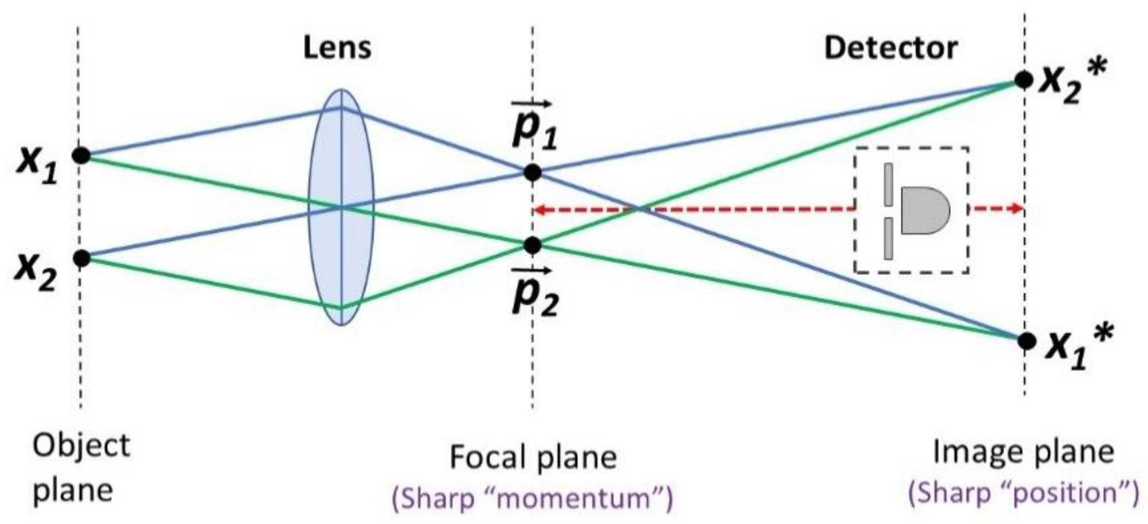
Figure 2.
Classical system with sequential binary properties. A macroscopic arrow is forced by a clockwork mechanism to rotate at a constant rate. (a) A full rotation produces two passages over each axis, as shown in the background. The opposite ends of each axis can be marked with binary values, such as “+” or “−”. (b) A CHSH arrangement can be produced by dividing the background plane into 8 sectors, containing the ordered measurement outcomes for the 4 relevant observables. It is possible to make two copies of this system, one for Alice and one for Bob. Yet, the value of this example is to illustrate the relationships between these 4 variables as part of a single mechanism. Each observable “becomes real” when the arrow passes above the corresponding sector. Maximal Bell violations emerge if pairs of events are detected in coincidence windows that include only two events at a time.
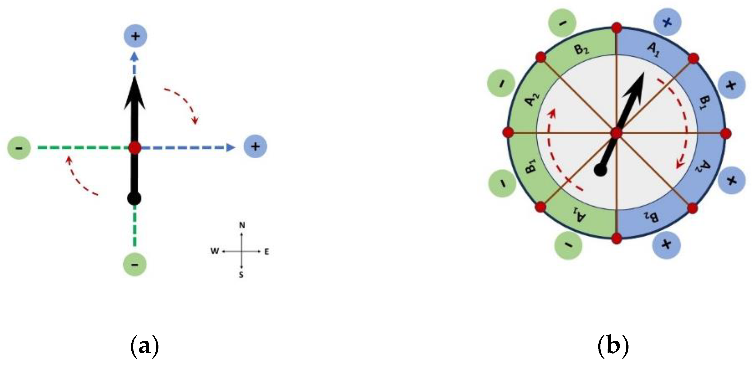
Figure 4.
Energy redistribution with incompatible outcomes. Classical velocity vectors can be decomposed into virtual pairs of components that correspond to the expected new value in any direction, in the event of a lossless elastic collision. The amounts of corresponding “available momentum” in each direction are proportional to the cosine of each angle of deflection. Yet, the redistributed amounts of kinetic energy are proportional to the cosine squared of the same angles. (a) An elastic collision at 45° between two billiard balls on a slate table results in a transfer of 50% of the input amount of energy. (b) The same final direction of motion can be achieved with two sequential collisions at 22.5° each. Yet, the final amount of energy in this case is 72%. It is not possible to reconcile the effect of two operations of redistribution at 22.5° with a single operation at 45°. This fundamental incompatibility between alternative outcomes is the source of Bell violations, both at the classical and the quantum level.
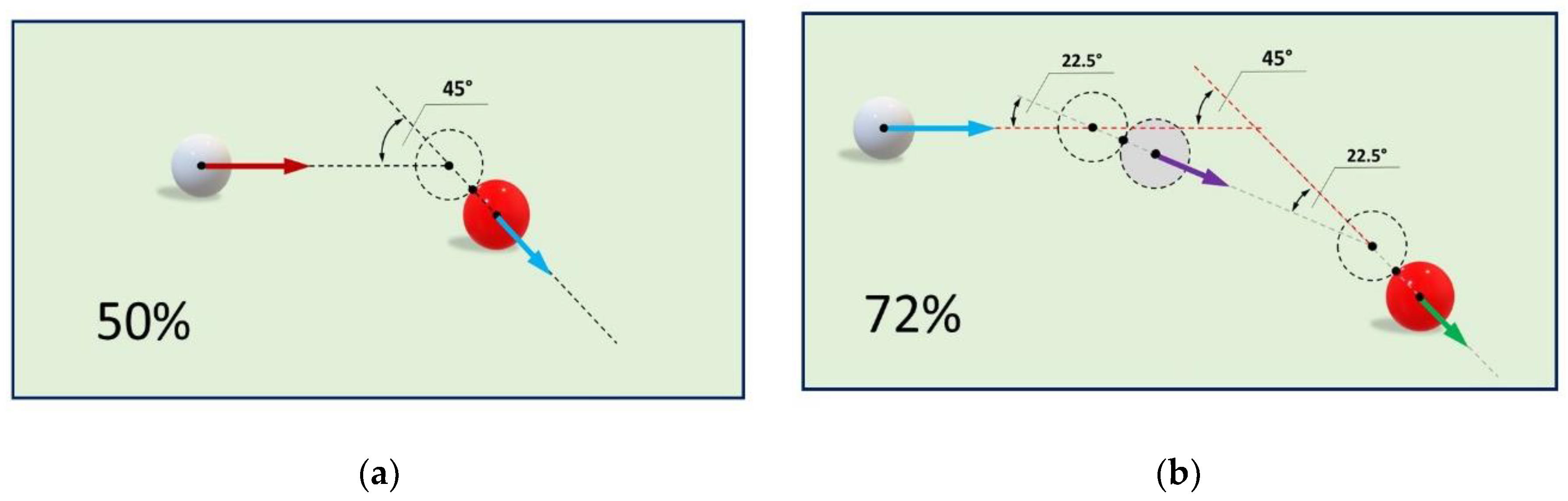
Figure 5.
Classical analogue for Stern-Gerlach electron behavior. CHSH experiments require alternative incompatible properties and rotational invariance for Bell violations. These conditions are satisfied by energy redistribution patterns in fluid flow-splitters. (a) Basic diagram of the mechanism. Fluid flows downward in the input pipe and is redistributed 50-50 between the two output pipes. The horizontal section is flexible, relative to the vertical channel. It can be rotated at will in the x-y plane. For any two directions, some fluid molecules will emerge through the same output pipe, and others will trade places. The proportion of identical outcomes is proportional to the cosine squared of half the angle between two randomly selected directions. This can be used to make a Bell experiment, by simulating two identical systems with microscopic precision in adequate computers. (b) Visual aid for understanding the possible combinations in a CHSH experiment. Alice can switch at random between two orthogonal orientations (A1 or A2), while Bob alternates between the other two (B1 or B2). Only four combinations are possible, such that three of them are separated by 45° and one by 135°. The end result is a quantum-like Bell violation.
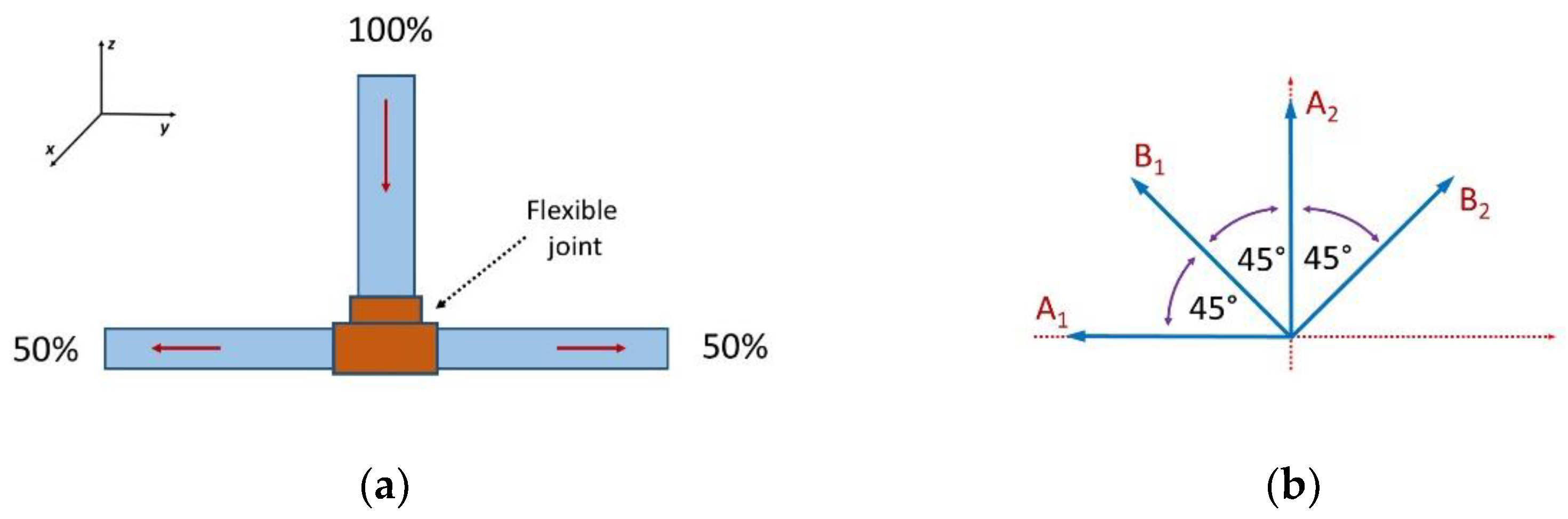
Figure 6.
“Monogamous” correlations with fixed predetermined outcomes. Bell violations require incompatible combinations of coefficients of correlation. In the CHSH protocol, this can be achieved with pairwise measurements, but not with quadruple measurements. The mechanism is revealed with sequential properties that manifest like clockwork. (a) A closed chain of pairwise measurements can produce a Mobius-strip pattern, such that three coefficients of correlations are compatible, and one is incompatible. This is achieved by maintaining a narrow window of coincidence for pairwise detection. (b) Quadruple detection requires a wider window of coincidence, breaking the pairwise flow of events. Three pairs of events are still coupled with the nearest neighbors, but one is paired “against the grain”. The same predetermined events are recorded, but the method of observation changes the pattern of combination.
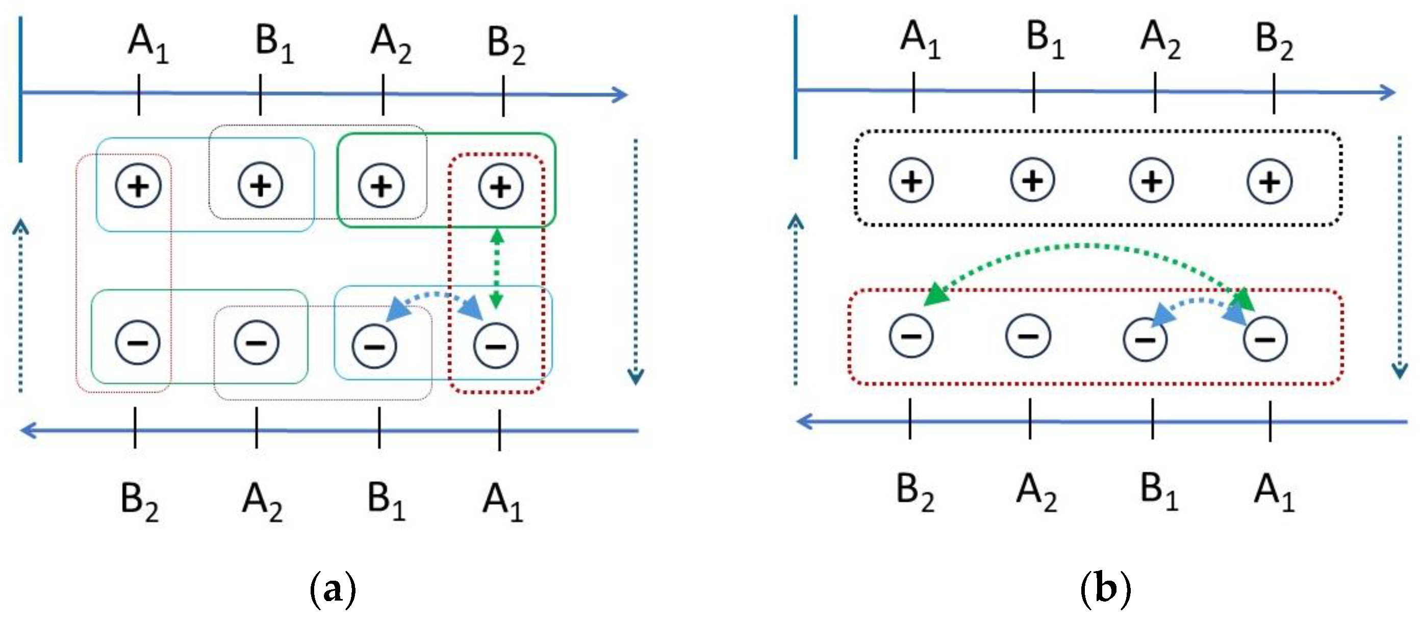
Disclaimer/Publisher’s Note: The statements, opinions and data contained in all publications are solely those of the individual author(s) and contributor(s) and not of MDPI and/or the editor(s). MDPI and/or the editor(s) disclaim responsibility for any injury to people or property resulting from any ideas, methods, instructions or products referred to in the content. |
© 2024 by the authors. Licensee MDPI, Basel, Switzerland. This article is an open access article distributed under the terms and conditions of the Creative Commons Attribution (CC BY) license (http://creativecommons.org/licenses/by/4.0/).
Copyright: This open access article is published under a Creative Commons CC BY 4.0 license, which permit the free download, distribution, and reuse, provided that the author and preprint are cited in any reuse.


