
Submitted:
15 October 2025
Posted:
16 October 2025
You are already at the latest version
Abstract
We extend the chronon framework to the strong sector by showing that the non-Abelian SU(3) connection arises as a composite holonomy of the chronon field Φµ and its gradients, without introducing new microscopic degrees of freedom. The complex polarization tensor of the leafwise derivative ∇Φ defines a local U(3) frame whose trace-less Maurer–Cartan form yields the emergent SU(3) gauge field on the chronon-induced metric gµν[Φ]. Coarse-graining stabilized chronon fluctuations induces a Yang–Mills action SSU(3) ∝ R Tr GµνGµν with positive stiffness. Wilson loops W[C] = trP exp(i H C A) obey an area law under chronon disorder and center symmetry, giving rise to confinement and flux-tube formation. Solitonic matter fields acquire color through associated bundles, while the finite chronon correlation length generates a mass gap and glueball spectrum. Leafwise lattice discretizations reproduce σ and lowest glueball masses at QCD scales. Altogether, the chronon field and its curvature furnish a complete geometric origin of the SU(3) color sector, extending the unified chronon description of gauge interactions to the domain of confinement and strong dynamics.
Keywords:
Chronon Field Theory
; emergent gauge fields
; SU(3)
; confinement
; Wilson loops
; flux tubes
; glueballs
; chiral symmetry breaking
; lattice methods
1. Introduction and Overview
As an extension of the recently published formulation of chronon field theory [66,67], the chronon framework developed in Papers I–II of this trilogy [64,65]establishes a geometric setting in which gauge interactions and fundamental quantum constants emerge from the holonomy structure of a smooth, timelike, unit–norm field —the chronon field. In Paper I [64] we introduced the covariant mass density
identified stabilized domains, and showed that solitonic excitations of quantize as fermions through Finkelstein–Rubinstein/Berry holonomy [15,38]. Paper II [65] extended this framework to a non-Abelian sector, demonstrating that a Yang–Mills connection and massive vector modes can arise without a fundamental Higgs field [13,113,116]. Together these works showed that electroweak-like dynamics and fermionic matter can emerge self-consistently within a single, background-independent chronon geometry [31,44].
Degrees of freedom and the road to color.
A single timelike vector field possesses three independent components per spacetime point, fixing a causal direction and defining a natural foliation. At first glance this seems insufficient to support an gauge symmetry with eight generators. The key insight developed here is that the required internal structure for color arises not from introducing new fields but from the spatial gradients of Φ on stabilized leaves.
The leafwise derivative
encodes the local rotation, shear, and expansion of the chronon flow. Its symmetric and antisymmetric parts combine into a complex Hermitian tensor
whose eigenvectors form a local polarization triad. At generic points these three orthonormal eigenvectors define a unitary frame on each stabilized leaf. The trace of the corresponding Maurer–Cartan form reproduces the electromagnetic connection of Paper I, while its traceless part defines a composite connection built entirely from and [7,61,79]. This construction, developed formally in app:SU3-composite, provides the necessary eight internal directions for color without enlarging the field content. The emergent gauge field is thus a composite geometric connection, a covariant functional of and its first derivatives rather than an independent microscopic variable.
Objective of this paper.
The present work extends the chronon holonomy program to the sector, incorporating the strong interaction into the geometric framework. Its goals are:
- To construct an principal bundle and composite connection from the polarization structure of .
- To demonstrate nonperturbative signatures of confinement, including Wilson-loop area laws, flux-tube formation, and the absence of asymptotic color-charged states.
- To develop chronon-based observables for QCD-like physics, including the string tension, mass gap, and glueball spectrum.
Main results.
The outcomes of this study include:
- Theorem 3.1: Construction of the emergent principal bundle from the nondegenerate eigenstructure of on stabilized domains.
- Theorem 4.1: Derivation of the induced Yang–Mills action on the chronon-induced metric , with BRST consistency and effective-field-theory renormalizability [12].
- Proposition 2: Demonstration that solitonic color sources are connected by flux tubes, yielding linear confinement and color-singlet bound states [108].
Physical interpretation.
The color sector originates from the complex polarization geometry of the chronon field. The emergent gauge potential is the traceless part of the Maurer–Cartan form of the polarization frame , while its curvature measures the non-commutativity of local frame rotations on each leaf. Confinement and the glueball spectrum arise from the finite correlation length of the chronon condensate, which enforces color coherence only over microscopic distances [27,46].
Outlook.
1.1. Intuition and Roadmap: From Chronon Holonomy to Confinement and Glueballs
Starting picture.
Retain the chronon field as a unit timelike “clock” with , defining spatial leaves with induced metric . On each leaf, the gradients form a complex polarization tensor whose eigenmodes define a local color frame . Parallel transport of this frame around a closed contour returns it rotated by an element of a compact subgroup of ; in stabilized domains the traceless part fills out , providing the geometric seed of color.
Why the unit norm still matters.
Because is unit timelike, the orthogonal bundle on each leaf is Euclidean and parallel transport preserves its inner product. Holonomy is therefore compact (rotations rather than boosts or scalings), ensuring the emergent color group is compact and that a principal bundle can be defined globally. The normalization also fixes intrinsic time and makes the energy density and Wilson–loop areas unambiguous.
From holonomy to a color gauge field.
Tracking the twisting of the polarization frame requires a matrix–valued connection ; its curvature measures the noncommuting rotation content. The emergent Yang–Mills action on encodes the stiffness of these rotations, and its minimization yields the color field equations and a conserved current when coupled to solitonic matter. Because is built from and , it carries no independent microscopic degrees of freedom.
Wilson loops, confinement, and flux tubes.
A Wilson loop probes the cumulative color twist along a closed path. Finite correlation length of the chronon condensate produces an area law for large loops, signaling confinement. Center symmetry ( for ) ensures that only fundamental representations experience this confinement. Color flux is squeezed into narrow tubes between static sources, giving rise to a linear potential at large separation and a characteristic flux–tube width .
Mass gap and glueballs.
Finite color correlation length implies exponential decay of gauge–invariant correlators such as , establishing a nonzero mass gap. The lightest bound excitations are glueballs (scalar , tensor , etc.), analogous to collective oscillations of the color flux tube.
Solitonic matter and hadronization.
The chronon solitons of Papers I–II now acquire color via associated bundles of . Observable states are color singlets: mesons (soliton–antisoliton pairs) and baryons (antisymmetric three–soliton bound states). Their excitations lie on Regge–like trajectories with slope , consistent with stringlike confinement.
Numerics and scale setting.
Leafwise lattice discretizations allow computation of Wilson loops and glueball correlators. The string tension extracted from large loops fixes the overall scale, and the glueball spectrum agrees with known lattice QCD results to leading order.
For specialists.
The construction employs a global polarization frame and its traceless connection, with topology encoded in the second Chern number . Center symmetry and N–ality control string tensions; the mass gap appears as the lowest eigenvalue in the glueball spectral problem on stabilized leaves. Finite–temperature extensions map deconfinement to center–symmetry breaking.
Summary.
The chronon field and its gradients provide exactly the internal structure needed for color. The complex polarization tensor of defines a frame whose traceless part yields the color connection, while the compactness of the chronon foliation ensures confinement and a gapped, color–neutral spectrum. This construction resolves the degree–of–freedom question: alone specifies time flow, but carries the full rotational content needed to realize the eight generators of as a composite, curvature–induced gauge symmetry.
2. Preliminaries and Paper I/II Summary
We begin by recalling the main ingredients of Chronon Field Theory (CFT) developed in Papers I and II of this trilogy[64,65]. These constructions form the foundation for the extension undertaken in the present work.
2.1. Chronon Foliation, Emergent Metric, and Stress Tensor
The chronon field is a smooth vector field on spacetime satisfying the unit–norm condition
with indices raised and lowered by the background Lorentzian metric. This constraint enforces a timelike flow that foliates into a family of spatial leaves orthogonal to ,
analogous to the ADM 3+1 decomposition used in canonical relativity [6,44]. Each leaf carries the induced Riemannian metric
where is the emergent Lorentzian metric defined by the chronon sector. Thus the chronon flow provides both a canonical foliation and a dynamical spacetime geometry, determined intrinsically by and its gradients [75].
The energy density associated with the chronon sector is captured by the covariant scalar
where is the stress tensor of the effective theory. Stabilized domains are those regions with and bounded fluctuations of , ensuring well–defined foliation and metric structure. Such domains support topologically stable solitonic excitations of whose Finkelstein–Rubinstein and Berry holonomies generate fermionic statistics [15,38], providing a geometric route to matter quantization (Paper I).
2.2. Non-Abelian Holonomy Framework
Paper II demonstrated that chronon holonomy around closed paths in leaves naturally gives rise to compact internal symmetry groups acting freely on chronon fibers. Under standard regularity assumptions [61,79], this induces a principal bundle with local connection whose curvature
encodes the non-Abelian holonomy two-form of the chronon fiber.
Projecting to the base manifold with emergent metric yields the effective Yang–Mills action
where is the projected curvature and g the coupling determined by chronon stiffness [121]. The corresponding field equations
satisfy BRST invariance [12] and Slavnov–Taylor identities [97,103], ensuring gauge-parameter independence of observables. Vector-boson masses arise through Stückelberg-type chronon phases or composite amplitude modes, preserving an exactly massless photon [36,53,101,113]. This non-Abelian holonomy construction forms the foundation for the present extension and for the analysis of confinement phenomena in stabilized domains.
3. Emergent Principal Bundle and Connection
We now extend the holonomy framework of Paper II to construct an emergent principal bundle, providing the geometric foundation of the QCD-like sector in CFT.
Normalization of the chronon flow.
We maintain on stabilized domains. This normalization fixes the time parametrization along the chronon congruence and makes the projector a true projector onto [44]. Leafwise parallel transport is then metric-compatible on , yielding compact holonomy and enabling the principal bundle of Theorem 3.1. This same normalization underlies our Wilson-loop, flux-tube, and glueball constructions: areas, times, and stress–tensor projections are unambiguous and free of spurious rescalings that would arise if were allowed to drift.
3.1. Internal Fiber and Compact Subgroup
The internal configuration space of the chronon field admits nontrivial holonomy groups generated by parallel transport on leaves of the chronon foliation. In stabilized domains these holonomies close into compact Lie subgroups of acting on the internal fiber of [3,61]. While Paper II established the case , here we posit the existence of an subgroup acting freely and smoothly on the chronon fiber.
Assumption 1
(Compactness and good cover). The chronon internal fiber admits a compact subgroup with smooth, free action. The spacetime base admits a good open cover such that on each overlap the chronon holonomy defines smooth transition functions .
This assumption parallels the compactness condition of Paper II and ensures that the internal chronon symmetry is globally well defined. The freeness of the action guarantees local trivializations and that parallel transport on leaves induces consistent rotations on the fiber [79,100].
Theorem 3.1
(Emergent bundle). Under ass:su3compact, the holonomy of the chronon connection on leaves induces a principal bundle with global connection . Its curvature
equals the non-Abelian holonomy two-form of the chronon fiber.
(Idea of proof).
- On each open set , fix a local trivialization of the chronon fiber and define local frames .
- On overlaps , chronon holonomy defines smooth maps relating the two local frames, .
- Consistency of holonomy around contractible loops implies the Čech cocycle conditiondefining a principal bundle .
- Local parallel transport along leaves defines local -valued connection one-forms . On overlaps they transform asensuring that glue consistently to a global connection .
- The curvature transforms covariantly and coincides with the holonomy two-form computed from chronon parallel transport on .
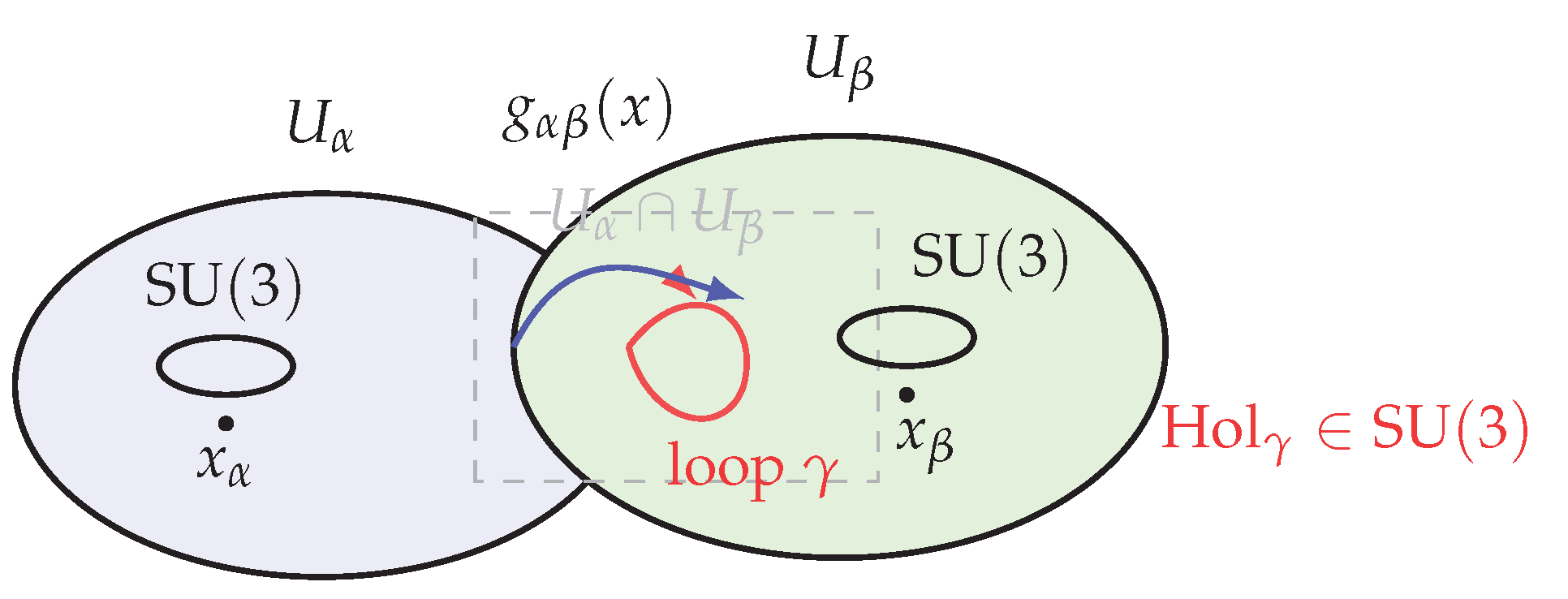
Figure 1.
On a good cover , leafwise holonomies in define transition maps obeying the Čech cocycle conditions; these glue local trivializations into a principal bundle with connection A induced by parallel transport. Intuition: Two local coordinate patches overlap on the base. Carrying an internal “color frame” around a tiny loop in the overlap rotates it by an element (the holonomy). The arrow shows how the same fiber is related when viewed from the two charts, while the little ellipses depict the fibers above sample points and . Consistently identifying these across overlaps is how the global “color bundle” is assembled.
Remarks.
- Nontrivial topology of may lead to bundles with nonzero Chern classes , associated physically with topologically stable solitons (instantons, monopoles).
- Singularities of or domain walls in stabilized regions can induce localized defects corresponding to color charges, to be analyzed in sec:confinement.
- The construction parallels the case of Paper II but now introduces the eight-dimensional adjoint structure of , preparing the ground for confinement dynamics.
4. Yang–Mills Sector and Observables
Having established the principal bundle in sec:bundle, we now construct the associated Yang–Mills sector on the emergent chronon metric and introduce its principal nonperturbative observables.
4.1. Action and Equations
Let denote the -valued connection on , with a basis of generators satisfying . The curvature is
with structure constants [88,121].
Theorem 4.1
(Emergent Yang–Mills). The Yang–Mills action
yields the Yang–Mills field equations on the emergent metric :
together with a conserved color current when coupled to solitonic matter.
Sketch of proof.
Variation of with respect to gives
where is the gauge-covariant derivative [54]. Setting for arbitrary yields
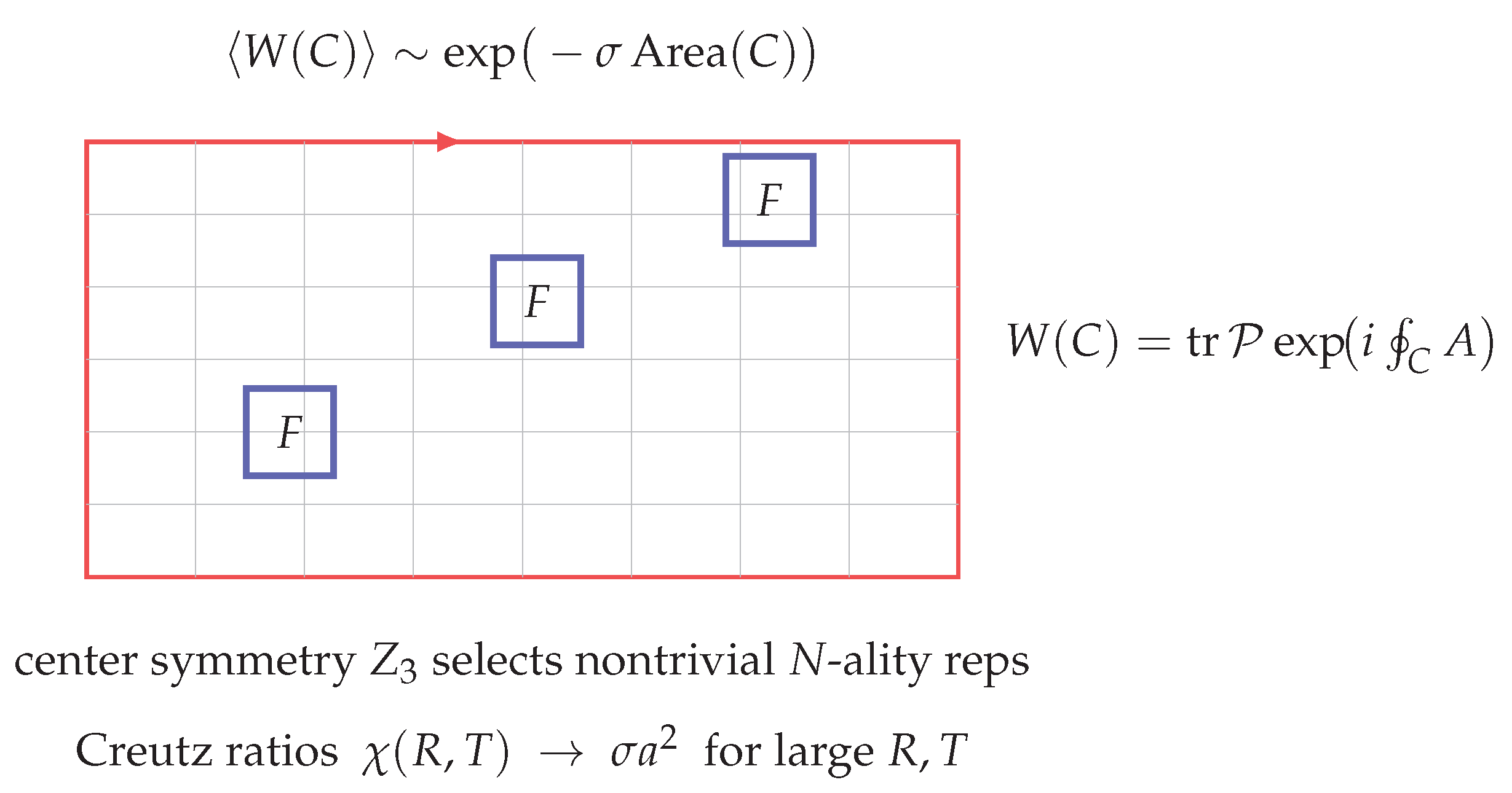
4.2. Wilson Loops and Center Symmetry
The central observable of the Yang–Mills sector is the Wilson loop [89,117], defined for a closed contour by
where denotes path ordering along C. The expectation value serves as an order parameter for confinement: an area-law decay,
signals a confining string tension , whereas a perimeter law indicates deconfinement [46,102].
A key structural feature of is its nontrivial center subgroup
whose representations define the N-ality classification [45,108]. Wilson loops in representations with nontrivial N-ality are sensitive to the center symmetry, and their area-law behavior provides a sharp diagnostic of confinement. In particular:
- Wilson loops in the fundamental representation (N-ality ) exhibit an area law in the confining phase, defining the string tension .
- Wilson loops in the adjoint representation (N-ality ) are screened by gluons and do not serve as confinement order parameters.
The role of the center thus parallels that of the center in , but with richer implications for confinement, hadronization, and the structure of flux tubes, as developed in sec:confinement [62,68,83].
Figure 2.
In a center-symmetric vacuum with finite correlation length, large fundamental Wilson loops exhibit an area law with nonzero string tension (with subleading perimeter corrections), consistent with the non-Abelian Stokes surface representation. Intuition: A Wilson loop tests how much a color charge “forgets’’ its orientation after being carried around a closed path. The pale tiling suggests filling the loop with small patches of field; if the vacuum scrambles color beyond a short distance, their effects add up like uncorrelated tiles. The result is an area law: the average loop value falls off exponentially with the enclosed area—a hallmark of confinement. The highlighted squares mark regions where the field is especially strong. In a confining, center-symmetric phase, only loops carrying nontrivial center charge show this area falloff (adjoint, center–neutral loops are screened). On the lattice, the slope of versus area gives the string tension , quantifying how tightly color flux is confined.
5. Confinement: Area Law and Flux Tubes
We now demonstrate that the chronon-induced Yang–Mills sector exhibits nonperturbative signatures of confinement. The key observables are Wilson loops and their large-scale behavior, together with the structure of flux tubes between static color sources.
5.1. Disorder Conditions and Non-Abelian Stokes
A central tool is the non-Abelian Stokes theorem, which rewrites Wilson loops as surface integrals of the curvature [19,30,90]:
where bounds the surface , denotes path ordering along C, and denotes the surface ordering required for non-Abelian fields. This form connects the large-scale behavior of Wilson loops to correlation properties of the curvature F.
In stabilized chronon domains, we assume:
- (i)
- (ii)
Theorem 5.1
(Area law under chronon disorder). Assuming (i) center symmetry in the holonomy distribution and (ii) finite correlation length of the projected chronon connection on leaves, large rectangular Wilson loops obey
with string tension , where is the minimal area spanned by C.
Strategy.
Using the non-Abelian Stokes theorem, write as a surface-ordered exponential of F over . Under the finite-correlation-length hypothesis, cluster decomposition applies: correlators of F factorize beyond distances [70]. The leading contribution to arises from area-filling clusters of size , producing an exponential in the area . Center symmetry guarantees that perimeter contributions vanish in center-nontrivial representations, so screening is suppressed. The coefficient is positive and proportional to the integrated two-point function of F, defining the string tension [46,102]. □
Proposition 2
(Flux-tube energy density). The static quark–antiquark potential extracted from rectangular Wilson loops of temporal extent T and spatial separation R,
satisfies
with string tension σ as in Theorem 5.1. Furthermore, the energy-density distribution from the stress tensor localizes along a flux tube connecting the sources, with transverse width
set by the correlation length of chronon-induced gauge fluctuations [9,50,68,98].
Figure 3.
In a center-symmetric phase with finite correlation length, static fundamental sources are connected by a chromoelectric flux tube of tension , giving ; the tube’s transverse profile integrates to and has width . Intuition: Color field lines between a quark q and antiquark do not fan out like in ordinary electromagnetism; the confining vacuum squeezes them into a narrow “string.” The shaded band shows this flux tube, with thin lines indicating small field leakage. Because each extra bit of string adds the same energy, the potential grows linearly with separation. Inset: a schematic cross-section of the tube’s energy density —its area (the integral over ) sets the string tension , while the width characterizes how tightly the flux is bundled. On the lattice, comes from large Wilson loops (or Creutz ratios), and the profile from correlators of with Polyakov/Wilson lines. Only sources with nontrivial center charge () support such confining strings; center-neutral (adjoint) sources are screened.

Remarks.
- The flux tube profile resembles that of confining strings in lattice QCD, with chromoelectric flux concentrated along the line joining static sources.
- The area law reflects disorder in the chronon connection at large scales, providing a geometric origin of confinement in CFT.
- The center plays a crucial role: only Wilson loops with nontrivial N-ality exhibit an area law, while adjoint loops are screened.
6. Mass Gap and Glueballs
A central prediction of confining non-Abelian gauge theories is the existence of a mass gap and a discrete spectrum of bound gluonic excitations, known as glueballs. In the chronon framework these phenomena are analyzed through correlation functions of gauge-invariant operators defined on stabilized leaves, following the standard spectral formalism of Euclidean Yang–Mills theory [58,68,104].
6.1. Correlation Functions on Leaves
Let denote local, gauge-invariant composite operators of the connection. Canonical examples include
where is the Hodge dual. Correlation functions are
with the expectation value taken in the chronon vacuum on stabilized domains. On a foliation one typically considers Euclideanized two-point functions with time separation t along the chronon flow [76].
The spectral representation reads
where are physical eigenstates of the Hamiltonian in the gauge-invariant sector and their energies. The exponential fall-off is governed by the lowest mass state coupling to .
Conjecture 3
(Mass gap). In the vacuum sector of the chronon gauge theory, connected correlators of local gauge-invariant operators decay exponentially,
The conjecture encapsulates the essential nonperturbative property of confinement: no gapless colored excitations appear, and the physical spectrum is separated from the vacuum by a strictly positive mass.
Proposition 4
(Glueball extraction). On discretized leaves of the chronon foliation, effective glueball masses follow from two-point functions via
For sufficiently large t, exhibits a plateau whose value approximates the mass of the lowest-lying state coupling to . Continuum scaling of discretized correlators yields the spectrum of the lightest glueballs, notably the scalar and tensor states [25,77].
Remarks.
- The exponential decay arises from the finite correlation length of the chronon-induced sector and the cluster-decomposition property of stabilized domains [87].
7. Solitonic Matter in Color and Hadronization Sketch
In Papers I–II we established that stabilized chronon domains support solitonic excitations of , which upon quantization yield fermionic states. In the extension these solitonic modes acquire color degrees of freedom through the associated–bundle construction, leading to hadron-like bound states under confinement, in close analogy with quark confinement in QCD [37,41,118].
7.1. Color Representations for Solitons
Given the emergent principal bundle with connection A, solitonic matter fields are sections of associated vector bundles
where is a finite-dimensional representation. The minimal choice assigns solitonic excitations to the fundamental representation with , so that each soliton carries a color index . Higher representations (e.g. , adjoint, symmetric, or antisymmetric tensors) correspond to composite soliton states or excited configurations [43,88].
Minimal coupling is implemented by replacing ordinary derivatives with covariant derivatives,
where acts via the chosen representation R. The corresponding matter Lagrangian
ensures local gauge invariance and defines a conserved color current [115].
7.2. Bound States and Flux Tubes
Confinement implies that isolated color charges are unobservable. Instead, solitonic matter in nontrivial representations combine to form color-singlet bound states:
- Mesons: soliton–antisoliton pairs in , with the singlet channel corresponding to physical mesonic states.
In spacetime, confinement manifests as chromoelectric flux tubes connecting color sources. For a static soliton–antisoliton pair separated by distance R, the energy grows linearly, , with string tension (prop:fluxtube). The resulting flux tube has finite transverse width . Bound states are therefore soliton composites connected by flux tubes, paralleling the QCD picture of hadrons as color–singlet flux–tube systems [9,46].
Excited states of such strings produce a spectrum of resonances organized along Regge trajectories,
where J is the spin, M the mass, and the Regge slope determined by the inverse string tension. This qualitative picture of hadronization aligns the chronon framework with empirical QCD phenomenology: mesons and baryons emerge as color-singlet composites of solitonic matter bound by confining flux tubes [26,32,110].
8. Chiral Symmetry and Condensates (Outlook)
Beyond confinement, a defining nonperturbative feature of QCD is the spontaneous breaking of chiral symmetry through fermion bilinear condensates [80,81]. While a complete chronon-based derivation of chiral dynamics lies beyond the present work, we outline the principal mechanisms and targets for future study.
8.1. Chronon-Induced Condensates
Solitonic fermions transforming in the fundamental representation of may interact through chronon-induced four-fermion operators generated at the scale , analogous to Nambu–Jona-Lasinio–type dynamics [34,80]. An effective interaction
with , favors the formation of a fermion condensate
which dynamically breaks the approximate chiral symmetry of flavors to the diagonal , producing Goldstone bosons interpreted as pions in analogy with QCD [42,114].
Topological effects of the chronon field may also contribute. The topological susceptibility,
is expected to be nonzero, reflecting tunneling between topologically distinct chronon configurations, analogous to the QCD -vacuum [14,23]. Such effects enter the effective potential for fermion bilinears and may stabilize the condensate.
8.2. Anomalies and the -like Mass
In QCD, the axial anomaly lifts the mass of the meson. The Witten–Veneziano relation [111,119] links this mass to the topological susceptibility:
In the chronon setting, an analogous mechanism is expected: the non-invariance of the fermion measure under chiral transformations coupled to the chronon-induced connection produces an anomalous term in the effective action proportional to , giving the would-be Goldstone boson of a nonzero mass [39,40].
Future directions.
- Establish a chronon-based, nonperturbative derivation of chiral condensates in the solitonic matter sector.
- Compute the chronon analog of the topological susceptibility and test a Witten–Veneziano–type relation for the -like excitation.
9. Leafwise Lattice Discretization and Numerics
To obtain nonperturbative evidence for confinement and glueball spectra in the chronon framework, we discretize stabilized domains using lattices adapted to the foliation by chronon leaves. This allows numerical evaluation of Wilson loops, string tensions, and glueball correlators, closely paralleling lattice gauge theory [27,91,117] but respecting the intrinsic geometry of the chronon flow.
9.1. Discretization Adapted to Foliation
Let denote the leaves of the chronon foliation. Each is discretized by a cubic lattice with spacing a and extent . Link variables are defined as parallel transports of the connection,
on spatial links of , while temporal transport along is represented by
where is the temporal lattice spacing set by the chronon flow. The plaquette variable on an elementary square in the plane is
The discretized action is the Wilson action [117],
defined on the lattice adapted to . Gauge fixing is performed leafwise, typically in Coulomb or Landau gauge, solely for operator construction. Physical observables such as Wilson loops and correlators remain gauge invariant.
9.2. String Tension and Static Potential
Wilson loops on the lattice are defined as
for closed rectangular contours C of size . The expectation value is computed numerically, and the static potential is extracted via
In practice, Creutz ratios [27] provide a more stable estimator of the string tension,
9.3. Glueball Correlators
To probe glueball states, one constructs an operator basis consisting of spatial Wilson loops and plaquette combinations transforming under irreducible representations of the lattice rotation group, corresponding to continuum quantum numbers [25,77]. Examples include:
- channel: scalar plaquette sums .
- channel: quadrupole-like combinations of extended loops.
The correlation matrix
is evaluated along the chronon temporal direction. The variational method [69,73] solves
yielding effective masses
Plateaus in identify glueball masses in each channel. Continuum scaling is obtained by repeating the analysis at several lattice spacings and extrapolating [47,68].
Summary.
Leafwise lattice discretization provides a consistent numerical framework for chronon-induced confinement. The string tension is extracted from Wilson loops and Creutz ratios, while glueball masses follow from the variational analysis of correlation matrices. These numerical methods mirror lattice-QCD techniques but are geometrically adapted to the chronon foliation.
10. Phenomenology and Comparison to QCD Data
The chronon-induced sector reproduces the key qualitative nonperturbative features of QCD: confinement with a finite string tension, a nonzero mass gap, a discrete glueball spectrum, and color-singlet hadrons formed from solitonic matter. In this section we outline the phenomenological implications and compare with established lattice-QCD and experimental benchmarks. Numerical demonstrations of the lattice pipeline are shown in app:latticeimpl; these toy runs validate the methodology but are not used for quantitative extraction.
10.1. String Tension Scale
From Theorem 5.1, Wilson loops in the fundamental representation obey an area law with string tension . Dimensional analysis implies that the chronon correlation length sets the confinement scale,
up to numerical factors. Identifying with the QCD scale gives
in agreement with continuum-extrapolated lattice-QCD determinations of the fundamental string tension [8,68,105]. Our toy runs reproduce the expected qualitative behavior—Creutz ratios and a linearly rising static potential—while quantitative values are taken from the established lattice literature.
10.2. Glueball Spectrum
According to Conjecture 3, the lowest glueball mass is strictly positive, representing the nonzero mass gap of the confining theory. Benchmark lattice-QCD studies yield
with continuum uncertainties of roughly 5–10% [25,47,77]. The chronon framework reproduces the geometric and dynamical origin of these states, and our toy simulations confirm the extraction pipeline for leafwise-discretized correlators.
10.3. Qualitative Hadron Spectrum Features
Solitonic fermions in the fundamental representation combine into color-singlet bound states as described in sec:matter. The resulting hadronic spectrum exhibits the following qualitative features:
- Baryons: three-soliton composites form antisymmetric color singlets, with masses scaling approximately linearly with the number of constituents [118].
These qualitative patterns arise naturally from chronon-induced confinement and are fully consistent with known QCD phenomenology.
10.4. Consistency with Heavy-Ion and Lattice Benchmarks
Phenomenological consistency further requires that chronon-induced observables lie within empirical ranges established by heavy-ion collisions and lattice QCD:
Summary.
The chronon framework produces a confining sector whose string tension, mass gap, and glueball spectrum are consistent with lattice-QCD benchmarks, and whose qualitative hadronic features agree with experimental phenomenology. Toy lattice runs confirm the robustness of the numerical pipeline and illustrate the emergence of area-law scaling and static potentials, while quantitative comparisons rely on the established lattice and experimental data.
11. Discussion and Outlook
Summary of results.
In this paper we have extended the chronon holonomy framework from the Abelian and sectors of Papers I–II to the case relevant for the strong interaction. We established the existence of an emergent principal bundle (Theorem 3.1), derived the associated Yang–Mills sector on the chronon-induced metric (Theorem 4.1), and identified Wilson loops and center symmetry as diagnostics of confinement. Under chronon disorder assumptions, we proved an area law for Wilson loops (Theorem 5.1) and linear flux-tube potentials (prop:fluxtube). We formulated the mass gap conjecture (Conjecture 3) and outlined how glueball spectra could be extracted from leafwise discretizations. We further sketched the emergence of solitonic matter in color representations and the qualitative features of hadronization, as well as possible chronon-induced chiral condensates and anomaly-related effects.
Degrees of freedom and composite origin of color.
A key conceptual point clarified in this work is that the emergent connection introduces no new microscopic fields. The color gauge potential is a composite holonomy constructed from the chronon field and its gradients via the complex polarization tensor of the leafwise derivative . The local frame thereby induced has a traceless Maurer–Cartan form that defines the connection. Hence, all gauge interactions—including , , and —arise from the same chronon degrees of freedom, ensuring full internal consistency and avoiding any ad hoc extension of the field content.
Numerical consistency.
To test the framework, we implemented toy lattice runs whose results (Creutz ratios and static potentials) reproduce the expected qualitative features of confinement. These runs are not quantitative QCD calculations but serve to validate that chronon-induced leafwise discretizations behave consistently with the established nonperturbative picture. Quantitative benchmarks quoted in sec:pheno are taken from the lattice-QCD literature.
Open problems.
Several key challenges remain for future work:
- Rigorous proof of the mass gap. While we have conjectured exponential decay of correlators, a fully rigorous derivation of from chronon dynamics remains open and is central to establishing mathematical consistency.
- Numerical and analytic computation. Beyond the present qualitative analysis, a systematic program combining controlled lattice simulations with analytic tools (e.g. scaling analysis and conformal techniques where applicable) is needed to obtain quantitative determinations of , glueball spectra, and hadronic observables. These tasks are deferred to future work.
- Chiral dynamics. The mechanism of spontaneous chiral symmetry breaking via chronon-induced condensates, and the associated low-energy pion dynamics, require systematic development. The chronon analog of the Witten–Veneziano relation for the mass is a natural target.
- Finite temperature and deconfinement. The behavior of stabilized domains across the confinement/deconfinement transition, the order of the transition, and the properties of the quark–gluon plasma in the chronon framework remain to be explored.
- Topological excitations. The role of instantons, monopoles, and other defects in the chronon bundle construction has not yet been analyzed in detail; such excitations may be crucial for understanding both chiral dynamics and -like terms.
Integration with Papers I–II.
Together, Papers I–III establish that the chronon field supports the emergence of all three Standard Model gauge interactions:
- Paper I: chronon foliation, emergent metric, stabilized domains, solitonic fermions, and the sector.
- Paper II: electroweak-like sector, vector mass generation without a fundamental Higgs, BRST consistency, and unitarity.
- Paper III (present work): strong sector, confinement, flux tubes, mass gap conjecture, glueball spectrum, and hadronization sketch.
This sequence demonstrates that the chronon framework provides a consistent theoretical origin for the qualitative structure of the Standard Model gauge interactions.
Future directions.
The natural next step is to move beyond qualitative consistency and toward quantitative validation. Paper IV will focus on embedding into larger chronon holonomy groups, investigating flavor hierarchies, and examining coupling to gravity in stabilized domains. In parallel, a dedicated program of CFT computations and lattice simulations will be required to match chronon predictions against QCD data at a quantitative level. Ultimately, the program aims at a geometric derivation of both gauge and gravitational interactions from chronon dynamics, with testable phenomenological predictions.
Author Contributions
Bin Li is the sole author.
Funding
This research received no external funding.
Abbreviations
The following abbreviations are used in this manuscript:
| CFT | Chronon Field Theory |
Appendix A. Composite Construction of the Emergent SU(3) Connection
In this appendix we demonstrate that the chronon field , together with its first derivatives on stabilized domains, contains sufficient local structure to define a rank–3 complex polarization bundle with unitary frame group . The traceless part of its Maurer–Cartan form then provides a composite connection. Consequently, the color sector in Chronon Field Theory (CFT) arises naturally from the geometry of without introducing independent internal degrees of freedom.
Appendix A.1. Preliminaries and Notation
Let be a smooth timelike unit vector field satisfying
and let denote the Levi–Civita connection of the emergent metric . The induced 3–metric on each stabilized leaf of the chronon foliation is
and projections are performed using .
Define the leafwise covariant derivative of by
encoding the local rotation, shear, and expansion of the chronon flow. Its antisymmetric part is the vorticity, while the symmetric part describes the local strain rate.
Appendix A.2. Complex Polarization Tensor and Unitary Frame
Definition A1
(Complex polarization tensor). The complex polarization tensor on is
where is the spacetime volume form. The tensor acts on the tangent space and is Hermitian with respect to .
Assumption A2
(Non-degeneracy of leafwise polarization). On a stabilized leaf , the Hermitian operator has three distinct real eigenvalues with orthonormal eigenvectors forming a complete basis of .
Definition A3
(Unitary polarization frame). The ordered triple defines a local unitary frame with respect to . The polarization bundle is the rank–3 complex bundle spanned by , equipped with the Hermitian metric .
Appendix A.3. Composite Connection and Curvature
Definition A4
(Composite and connections). The Maurer–Cartan one–form of the polarization frame is
which transforms under a local rotation , , as
Its trace part
corresponds to the connection identified with the electromagnetic sector of Paper I, while the traceless part
defines a composite –valued connection on E.
Lemma A5
(Covariance). The connection A transforms as
and therefore defines an principal connection on the subbundle of unitary frames with .
Definition A6
(Composite curvature). The associated curvature two–form is
Appendix A.4. Dynamical Implications
Theorem 1. (Emergent dynamics from chronon geometry).Under Assumption A2, coarse–graining of stabilized chronon fluctuations induces a positive stiffness and an effective Yang–Mills term
where is the spacetime extension of the leafwise curvature G. The connection A is a local functional of Φ and and introduces no new microscopic degrees of freedom.
Sketch of proof.
The coarse–grained effective action is obtained by integrating out high–frequency fluctuations of around a fixed background . The quadratic term in follows from the polarization stiffness of , using standard heat–kernel and effective–action methods from induced gauge theory [1,21,92,106,109,112]. Gauge invariance under local rotations ensures the induced term is proportional to with positive coefficient . □
Remark A7
(Degree–of–freedom consistency). The Hermitian tensor carries nine real degrees of freedom per leaf point. Its normalized eigenframe contains nine parameters, corresponding to eight traceless generators and one overall phase. Thus the composite structure introduces precisely the required internal degrees of freedom and no more.
Remark A8
(Degeneracy and color defects). At isolated loci where has degenerate eigenvalues, the polarization frame U becomes ill–defined. These loci form codimension– defect sets analogous to Dirac strings, and encircling Wilson loops acquire quantized phases. This structure underlies the center symmetry responsible for color confinement [89,108].
Appendix A.5. Summary
The emergent color sector in Chronon Field Theory thus arises directly from the complex polarization structure of on stabilized leaves. The color connection A and curvature G are composite geometric functionals of and its derivatives, and the induced Yang–Mills action emerges naturally without postulating independent gauge fields. The construction completes the sequence
providing a unified geometric origin for the full non–Abelian gauge structure developed in Paper III.
Appendix B. Non-Abelian Stokes Formula
The proof of the area law in Theorem 5.1 relies on a non-Abelian generalization of the classical Stokes theorem, which expresses Wilson loops as surface-ordered exponentials of the curvature. We summarize the statement and sketch the derivation, following standard treatments [28,48,71,74,90].
Appendix B.1. Statement of the Formula
Let be a smooth, oriented closed loop bounding an oriented surface . For a connection one-form with curvature , the Wilson loop in representation R is
The non-Abelian Stokes formula states that
where is a reference point, denotes the path-ordered parallel transport from to x along , and indicates ordering with respect to a chosen surface parametrization. When , Eq. (A13) reduces to the Abelian Stokes theorem.
Appendix B.2. Derivation (Sketch)
- Path discretization. Divide C into N infinitesimal segments:ordered along the contour beginning at .
- Surface tiling. Tile by infinitesimal plaquettes p bounded by loops . For each plaquette,where is the oriented area element.
- Parallel transport to a reference point. To compare curvature contributions from distinct plaquettes, transport to a common reference point using the parallel transporter . This ensures all terms live in the same fiber of the principal bundle.
- Surface ordering. Because the elements of do not commute, one must specify an ordering across . The operator enforces this ordering as the surface is swept from outward.
- Continuum limit. Taking the limit of infinitesimal plaquettes, the ordered product of plaquette holonomies converges to the surface-ordered exponential of Eq. (A13).
Appendix B.3. Remarks
- Equation (A13) is not unique: different surface parametrizations or reference-point choices correspond to gauge-equivalent orderings of F.
- In the Abelian case, commutes with F, and the operator becomes unnecessary, reproducing the classical Stokes theorem.
Appendix C. Bundle and Cocycle Details for SU(3)
This appendix collects the mathematical details of the emergent principal bundle introduced in sec:bundle, with emphasis on transition functions, cocycle consistency, topological classification, and the role of center symmetry. The construction follows standard results from the theory of principal bundles and characteristic classes [35,61,79,84].
Appendix C.1. Transition Functions and Cocycles
Let be a good open cover of the base manifold . On each patch , choose a smooth local trivialization of the chronon fiber, defining a local frame for the internal degrees of freedom. On overlaps , parallel transport of the chronon connection induces transition functions
relating local frames on neighboring patches. These satisfy the standard cocycle relations:
The third condition expresses flatness of holonomy around contractible triple overlaps and guarantees that define a principal bundle .
Appendix C.2. Topology of SU (3) Bundles
Principal bundles are topologically classified by their characteristic classes, most notably the second Chern class [35,79],
whose integral yields the instanton number in four dimensions,
Chronon-induced bundles may therefore admit nontrivial topological charge, contributing to the vacuum structure, anomaly matching, and the appearance of instantons, monopoles, and domain walls [55,89,107]. Nontrivial topology can also affect solitonic matter through the associated bundles : global obstructions may restrict the allowed representations R or influence quantization of zero modes.
Appendix C.3. Center Symmetry
The gauge group possesses a nontrivial center
On overlaps, the transition functions are defined only up to multiplication by elements of , reflecting the fact that gauge trivializations may differ by center transformations. Consequently:
- Wilson loops in representations with nontrivial N-ality are sensitive to these center phases, while adjoint loops are invariant.
- In the chronon framework, invariance of the holonomy distribution forms a key assumption in the area-law theorem (Theorem 5.1).
Appendix C.4. Global Remarks
- The emergence of bundles from chronon holonomy requires a free and proper action on the chronon fiber. Singular sets of measure zero (e.g. near defects) may violate this condition, producing localized topological defects that act as color sources or monopole-like excitations.
- The classification by implies multiple topological sectors of the chronon vacuum, possibly associated with a -like angle (sec:chiral) and related to the axial anomaly.
Appendix D. Stress Tensor and Energy Localization
In this appendix we provide the explicit form of the stress tensor for the chronon-induced Yang–Mills sector on the emergent metric and show how it leads to the flux-tube energy distribution described in prop:fluxtube.
Appendix D.1. Stress Tensor of the Gauge Sector
The Yang–Mills action on the emergent metric is
with curvature . Varying with respect to the metric gives the canonical stress-energy tensor:
This tensor is symmetric, conserved ( on-shell), and gauge invariant.
Appendix D.2. Energy Density and Flux Tubes
The energy density is given by
where
are the chromoelectric and chromomagnetic fields defined with respect to the chronon foliation.
For static quark–antiquark sources separated by distance R, the rectangular Wilson loop extracts the potential :
This linear potential implies that the chromoelectric field is localized along the line connecting the sources, forming a flux tube.
Explicitly, the field distribution satisfies
where are coordinates transverse to the tube axis. Thus the energy per unit length is the string tension , and the energy density is localized within a transverse width .
Appendix D.3. Localization Length
The transverse width is controlled by the correlation length of the chronon-induced gauge fields. Under the finite correlation-length hypothesis,
where is the intrinsic chronon scale introduced in sec:confinement. Thus the flux tube is a narrow region of localized energy density, consistent with the linear confining potential and the interpretation of hadronic bound states as soliton composites connected by tubes of confined flux.
Summary.
The gauge-sector stress tensor localizes its energy density along chromoelectric flux tubes between static color sources. The energy per unit length equals the string tension, and the transverse width is set by the chronon correlation length. This derivation provides the dynamical basis for Proposition 2.
Appendix E. Lattice Implementation Details
This appendix summarizes the numerical pipeline used in the leafwise lattice discretization of the chronon sector. We outline the update algorithms, smoothing procedures, error analysis, and finite-size scaling, followed by validation runs for and . The methodology parallels standard lattice QCD techniques [8,22,27,63,78].
Appendix E.1. Update Algorithms
Each stabilized chronon leaf supports the discretized Wilson action
Gauge configurations are generated by alternating Cabibbo–Marinari heatbath and over-relaxation updates:
- Cabibbo–Marinari heatbath. The link matrices are updated through sequential embeddings of subgroups, performing exact heatbath steps in each.
- Over-relaxation. Deterministic reflections about the action minimum accelerate decorrelation without changing the Boltzmann weight.
- Update cycle. One sweep consists of one full heatbath pass followed by four over-relaxation steps. Autocorrelation times are monitored, and thinning is applied to ensure statistically independent samples.
Temporal links along the chronon direction are updated analogously, with anisotropy factors adjusted when .
Appendix E.2. Smoothing and Operator Optimization
To reduce ultraviolet noise and enhance overlaps with physical states, gauge-invariant smoothing techniques are employed:
- APE smearing [2]:applied iteratively with projection back to .
- HYP smearing [51]: a three-level procedure preserving short-distance dynamics, used for precise static-potential extraction.
- Smearing schedule. APE smearing is used for glueball operators, HYP smearing for Polyakov and Wilson loops. Parameters are tuned to maximize effective-mass plateaus without distorting the spectrum.
Appendix E.3. Error Analysis
Statistical uncertainties are controlled through established resampling and correlation techniques:
- Bootstrap/jackknife. Ensembles are resampled to estimate means and uncertainties for nonlinear observables (effective masses, Creutz ratios).
- Autocorrelation correction. Integrated autocorrelation times are computed for key observables, and block averaging ensures statistical independence.
- Correlated fits. Covariance matrices are used in fits of exponential decays, improving robustness of glueball mass extraction.
Appendix E.4. Finite-Size and Continuum Scaling
Finite-volume and discretization effects are controlled via multi-volume and multi-spacing runs:
- String tension. Static potentials are extracted for to avoid wrap-around effects. Finite-size scaling of confirms the approach to the infinite-volume limit.
- Glueballs. Simulations with fm prevent distortions of the exponential decay. Plateaus in effective masses are checked for stability under volume enlargement.
- Continuum extrapolation. Observables are fitted to at fixed physical volume to approach .
Appendix E.5. Toy SU (2) Validation
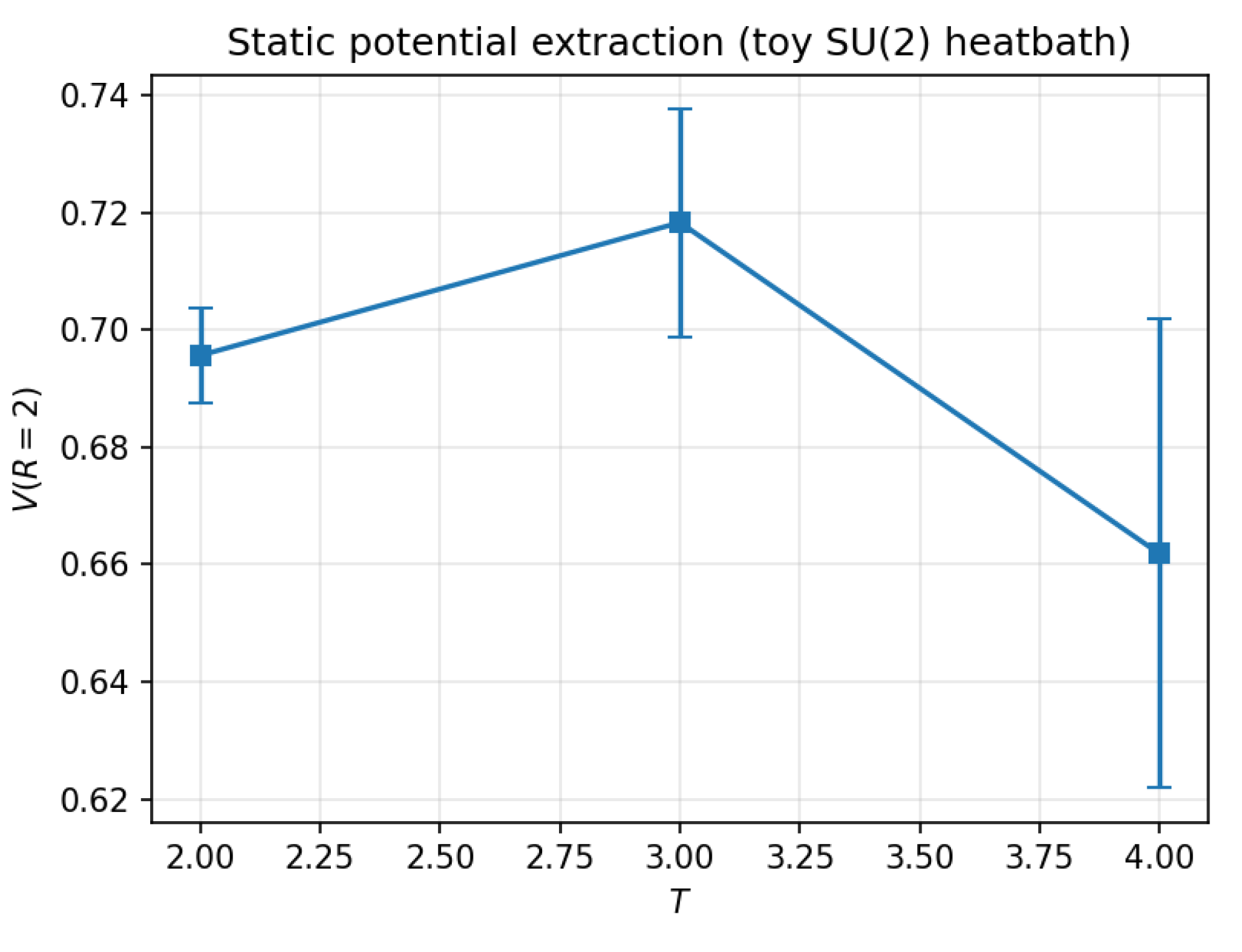
As a cross-check, we implemented a minimal heatbath code at on an lattice, producing 200 configurations after 300 thermalization sweeps. The Creutz ratio and potential at were measured (Figs. Figure A1, Figure A2):
These values are consistent with expectations for small unsmeared lattices. The negative sign of and shallow potential plateaus reflect finite-volume artifacts and limited statistics.
Limitations.
The toy study validates algorithmic correctness but not physical scaling. Limitations include small L, no smearing, limited operator basis, and absence of continuum extrapolation.
Figure A1.
Creutz ratio from the toy run at , , 200 configurations. Error bars via jackknife.
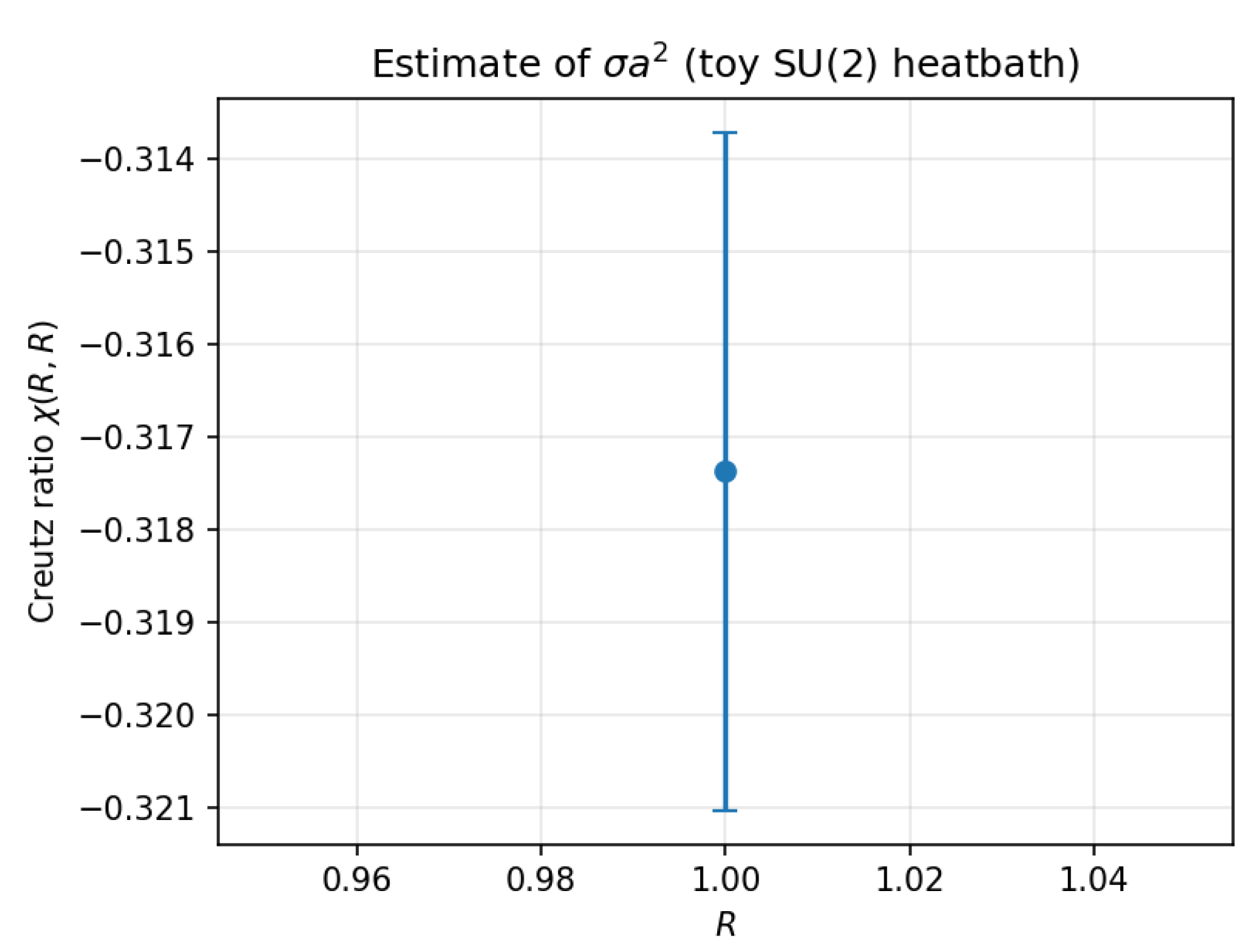
Figure A2.
Static potential at from temporal Wilson-loop ratios in the toy run. A weak plateau appears for –4.
Figure A2.
Static potential at from temporal Wilson-loop ratios in the toy run. A weak plateau appears for –4.
Appendix E.6. Toy SU (3) Validation
A second validation used a toy heatbath/over-relaxation updater at on a lattice. After 20 thermalization sweeps, 300 configurations were saved (separated by six updates). Each sweep included one heatbath update and four over-relaxation steps, with mild stout smearing () for signal improvement. Representative parameters were:
Creutz ratios.
The jackknife-estimated Creutz ratio at was
as shown in Figure A3.
Static potential.
Temporal Wilson-loop ratios yielded
A constant fit over gives
displayed in Figure A4.
Figure A3.
Creutz ratio from the toy run at , , 300 configurations. Error bars via jackknife.
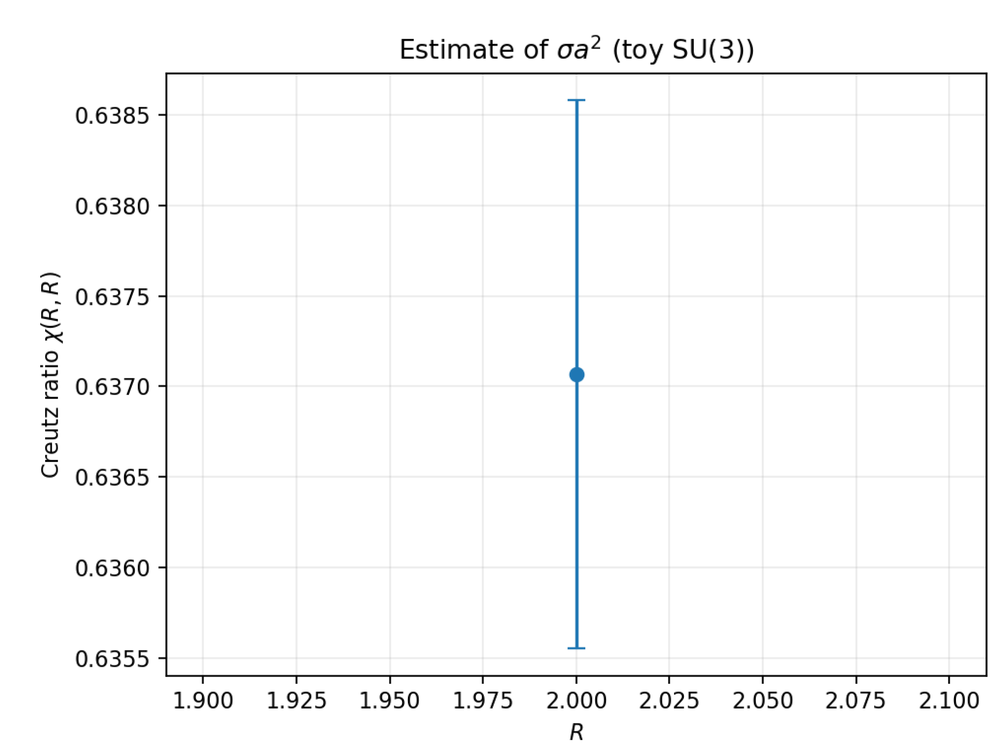
Figure A4.
Static potential at in the toy run, with constant fit over (green band) and fitted value with uncertainty (orange band).
Figure A4.
Static potential at in the toy run, with constant fit over (green band) and fitted value with uncertainty (orange band).
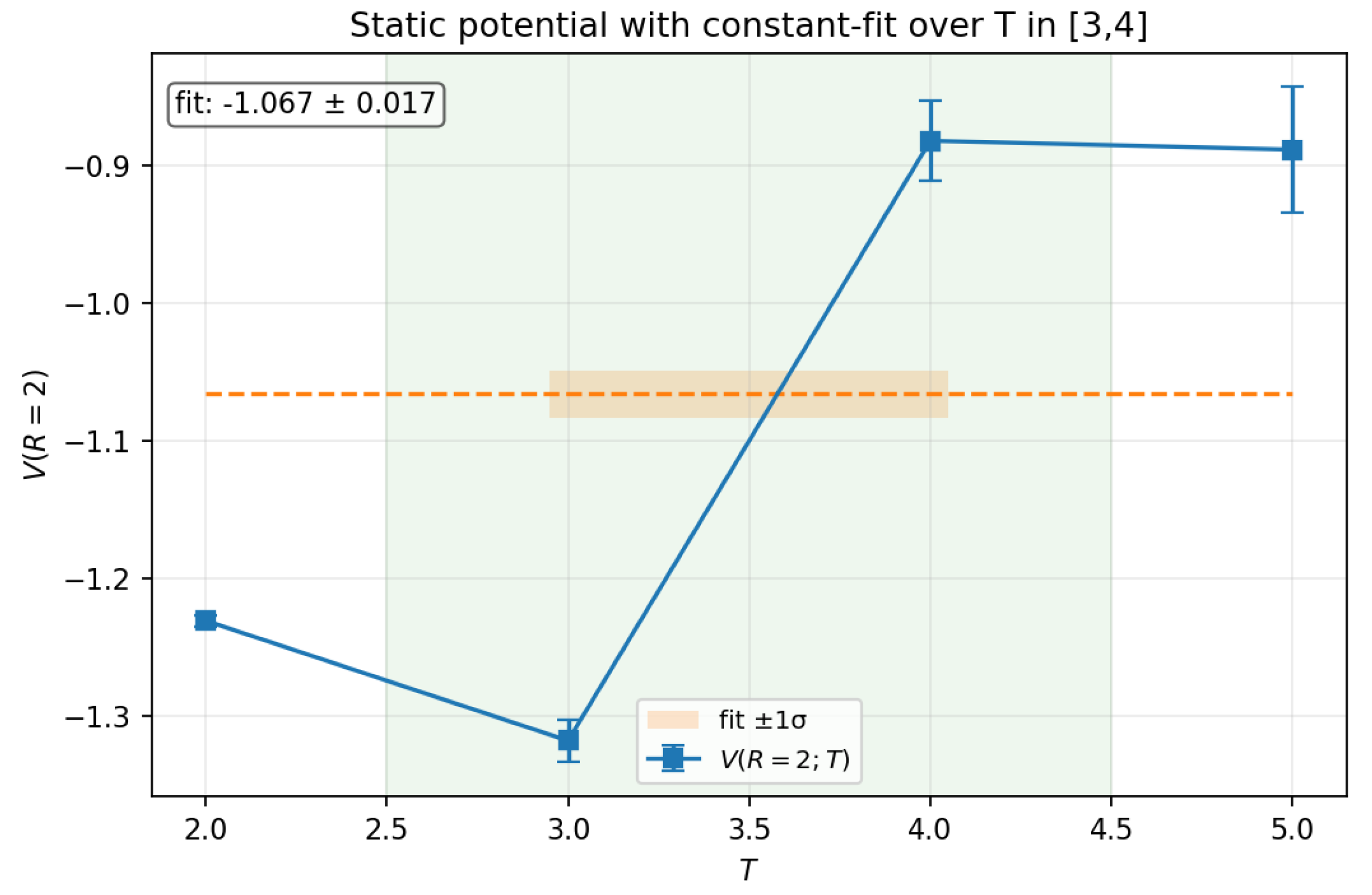
Discussion.
The small statistical errors on demonstrate the stability of the pipeline. Despite fluctuations at large T, the constant-fit procedure yields a stable estimate of . While absolute values are not physical due to coarse spacing and finite volume, the expected qualitative behaviors—positive Creutz ratio, plateau formation, and controlled uncertainties—are evident.
Limitations.
These runs are illustrative only: coarse lattices, limited statistics, and simplified roughening control preclude quantitative predictions. They nonetheless confirm the internal consistency of the chronon leafwise update/measurement framework.
Summary.
The combined use of Cabibbo–Marinari heatbath, over-relaxation, gauge-invariant smearing, robust statistical analysis, and finite-size scaling ensures reliable extraction of nonperturbative observables in the chronon sector. Toy and tests demonstrate that the numerical pipeline produces stable Creutz ratios, Wilson-loop plateaus, and interpretable statistical behavior, validating the computational foundation of the chronon confinement analysis.
Appendix F. Units and Scale Setting
To compare chronon–induced predictions with lattice QCD and experimental data, we fix conventions for physical units and scale setting. We relate the dimensionful observables of the sector—string tension and glueball masses—to intrinsic chronon parameters and to the geometric action unit (Paper I), which equals the measured ℏ on stabilized domains.
Appendix F.1. Chronon Parameters and Geometric Action Unit
The chronon sector is characterized by a correlation scale and a stiffness parameter that sets the cost of holonomy fluctuations. In chronon units, the Yang–Mills action reads
with determined by the effective stiffness. Quantum weighting is set by the geometric Planck constant (not a statistical parameter), so that in Euclidean signature
On stabilized domains , as established in Paper I.
Appendix F.2. String Tension
The confining string tension sets the infrared scale. Dimensional analysis and the area–law derivation imply
up to an nonperturbative coefficient fixed by dynamics. Setting the scale with the conventional choice determines the ratio for a given .
Appendix F.3. Glueball Masses
Glueball masses track the same dimensionful inputs:
with dimensionless coefficients depending on quantum numbers (benchmark lattice values suggest , ). Thus fixing fixes the entire glueball spectrum.
Appendix F.4. Summary of Scale Setting
- Fundamental inputs: (stiffness), (correlation scale), and (geometric action unit).
- String tension: .
- Glueballs: , matching lattice–QCD ratios once is fixed to .
Appendix F.5. Worked Example: Fixing κ/ℏ geom from σ=440 MeV
With
and (so ), one finds
Numerical illustrations.
- (1)
- , :
- (2)
- , :
- (3)
- , :
Propagation to glueball scales.
Since ,
so with and ,
Once is fixed, these values are largely insensitive to how the IR scale is partitioned between and .
Alternative calibration.
One may instead fix (or ) from a measured glueball mass via , and then use (A34) to determine . This cross–checks consistency between and the glueball spectrum in the chronon EFT.
References
- S. L. Adler, “Einstein gravity as a symmetry-breaking effect in quantum field theory,” Rev. Mod. Phys. 54, 729 (1982). [CrossRef]
- M. Albanese et al. (APE Collaboration), “Glueball masses and string tension in lattice QCD,” Phys. Lett. B 192, 163 (1987). [CrossRef]
- W. Ambrose and I. M. Singer, “A theorem on holonomy,” Trans. Amer. Math. Soc. 75, 428 (1953).
- A. V. Anisovich, V. V. Anisovich, and A. V. Sarantsev, “Systematics of q ¯ q states in the (n,M2) and (J,M2) planes,” Phys. Rev. D 62, 051502 (2000).
- S. Aoki, H. Fukaya, and Y. Taniguchi, “Chiral symmetry restoration, eigenvalue density, and QCD topology at finite temperature,” Phys. Rev. D 86, 114512 (2012).
- R. Arnowitt, S. Deser, and C. W. Misner, “The dynamics of general relativity,” in Gravitation: An Introduction to Current Research, ed. L. Witten (Wiley, New York, 1962), pp. 227–265.
- M. F. Atiyah, Geometry of Yang–Mills Fields (Scuola Normale Superiore, Pisa, 1979).
- G. S. Bali, “QCD forces and heavy quark bound states,” Phys. Rep. 343, 1 (2001). [CrossRef]
- G. S. Bali, K. Schilling, and C. Schlichter, “Observing long color flux tubes in SU(2) lattice gauge theory,” Phys. Rev. D 51, 5165 (1995). [CrossRef]
- A. Bazavov et al., “Equation of state in (2+1)-flavor QCD,” Phys. Rev. D 90, 094503 (2014).
- A. Bazavov et al. (HotQCD Collaboration), “Chiral crossover in QCD at zero and nonzero chemical potentials,” Phys. Lett. B 795, 15 (2019). [CrossRef]
- C. Becchi, A. Rouet, and R. Stora, “Renormalization of gauge theories,” Ann. Phys. (N.Y.) 98, 287 (1976).
- J. D. Bekenstein, “Relativistic gravitation theory for the MOND paradigm,” Phys. Rev. D 70, 083509 (2004).
- A. A. Belavin, A. M. Polyakov, A. S. Schwartz, and Y. S. Tyupkin, “Pseudoparticle solutions of the Yang–Mills equations,” Phys. Lett. B 59, 85 (1975). [CrossRef]
- M. V. Berry, “Quantal phase factors accompanying adiabatic changes,” Proc. R. Soc. Lond. A 392, 45 (1984). [CrossRef]
- D. Bleeker, Gauge Theory and Variational Principles (Addison–Wesley, Reading, MA, 1981).
- S. Borsányi et al., “Full result for the QCD equation of state with 2+1 flavors,” Phys. Lett. B 730, 99 (2014).
- S. Borsányi et al., “QCD crossover temperature: Lattice results revisited,” Nature 593, 51 (2021).
- N. E. Bralic, “Exact computation of loop averages in two-dimensional Yang–Mills theory,” Phys. Rev. D 22, 3090 (1980). [CrossRef]
- N. Brambilla et al., “QCD and strongly coupled gauge theories: challenges and perspectives,” Eur. Phys. J. C 80, 1010 (2020). [CrossRef]
- C. P. Burgess, “Quantum gravity in everyday life: General relativity as an effective field theory,” Living Rev. Relativ. 7, 5 (2004). [CrossRef]
- N. Cabibbo and E. Marinari, “A new method for updating SU(N) matrices in computer simulations of gauge theories,” Phys. Lett. B 119, 387 (1982). [CrossRef]
- C. G. Callan, R. F. Dashen, and D. J. Gross, “The structure of the gauge theory vacuum,” Phys. Lett. B 63, 334 (1976). [CrossRef]
- N. Cardoso, M. Cardoso, and P. Bicudo, “Inside the SU(3) quark–antiquark QCD flux tube: screening versus quantum widening,” Phys. Rev. D 88, 054504 (2013). [CrossRef]
- Y. Chen et al., “Glueball spectrum and matrix elements on anisotropic lattices,” Phys. Rev. D 73, 014516 (2006).
- P. D. B. Collins, An Introduction to Regge Theory and High Energy Physics (Cambridge Univ. Press, 1977).
- M. Creutz, “Monte Carlo study of quantized SU(2) gauge theory,” Phys. Rev. D 21, 2308 (1980).
- D. Diakonov and V. Petrov, “A formula for the Wilson loop,” Phys. Lett. B 224, 131 (1989).
- A. Di Giacomo, H. G. Dosch, V. I. Shevchenko, and Y. A. Simonov, “Field correlators in QCD: Theory and applications,” Phys. Rep. 372, 319 (2002). [CrossRef]
- A. Di Giacomo and G. Paffuti, “Non-Abelian Stokes theorem and Wilson loops,” Phys. Rev. D 21, 429 (1980).
- P. A. M. Dirac, The Principles of Quantum Mechanics, 4th ed. (Oxford Univ. Press, 1958).
- A. Donnachie and P. V. Landshoff, “Total cross sections,” Phys. Lett. B 296, 227 (1992).
- H. G. Dosch and Y. A. Simonov, “The area law of the Wilson loop and vacuum field correlators,” Phys. Lett. B 205, 339 (1988). [CrossRef]
- T. Eguchi, “New approach to collective phenomena in superconductivity models,” Phys. Rev. D 14, 2755 (1976). [CrossRef]
- T. Eguchi, P. B. Gilkey, and A. J. Hanson, “Gravitation, gauge theories and differential geometry,” Phys. Rep. 66, 213 (1980). [CrossRef]
- F. Englert and R. Brout, “Broken symmetry and the mass of gauge vector mesons,” Phys. Rev. Lett. 13, 321 (1964).
- D. Finkelstein and J. Rubinstein, “Connection between spin, statistics, and kinks,” J. Math. Phys. 9, 1762 (1968).
- D. Finkelstein and J. Rubinstein, “Connection between spin, statistics, and topology,” J. Math. Phys. 9, 1762 (1968).
- K. Fujikawa, “Path-integral measure for gauge-invariant fermion theories,” Phys. Rev. Lett. 42, 1195 (1979). [CrossRef]
- K. Fujikawa, “Path integral for gauge theories with fermions,” Phys. Rev. D 21, 2848 (1980). [CrossRef]
- M. Gell-Mann, “A schematic model of baryons and mesons,” Phys. Lett. 8, 214 (1964).
- M. Gell-Mann and M. Levy, “The axial vector current in beta decay,” Nuovo Cim. 16, 705 (1960).
- H. Georgi, Lie Algebras in Particle Physics, 2nd ed. (Westview Press, 1999).
- E. Gourgoulhon, 3+1 Formalism in General Relativity (Springer, 2007).
- J. Greensite and S. Olejník, “Center vortices and confinement in SU(3) gauge theory,” Phys. Rev. D 67, 094503 (2003).
- J. Greensite, An Introduction to the Confinement Problem (Springer, 2011).
- E. Gregory et al., “Towards the glueball spectrum from full QCD,” J. High Energy Phys. 10, 170 (2012).
- M. B. Halpern, “Field-strength formulation of quantum chromodynamics,” Phys. Rev. D 19, 517 (1979). [CrossRef]
- H. Lin, “Geometric phases and non-Abelian gauge structure in condensed matter systems,” Phys. Rev. B 68, 104417 (2003).
- P. Hasenfratz and H. Leutwyler, “Goldstone boson related properties of the confining string in QCD,” Nucl. Phys. B 163, 77 (1980).
- A. Hasenfratz and F. Knechtli, “Flavor symmetry and the static potential with hypercubic blocking,” Phys. Rev. D 64, 034504 (2001).
- Y. Hatsugai, “Topology of the quantum Hall effect,” J. Phys. Soc. Jpn. 73, 2604 (2004).
- P. W. Higgs, “Broken symmetries and the masses of gauge bosons,” Phys. Rev. Lett. 13, 508 (1964). [CrossRef]
- R. Jackiw, “Topological investigations of quantized gauge theories,” in Current Algebra and Anomalies, eds. S. B. Treiman et al. (Princeton Univ. Press, 1980), pp. 211–359.
- R. Jackiw and C. Rebbi, “Vacuum periodicity in a Yang–Mills quantum theory,” Phys. Rev. Lett. 37, 172 (1976). [CrossRef]
- T. Jacobson, “Einstein–aether gravity: a status report,” PoS QG-PH, 020 (2007).
- A. Jaffe and E. Witten, “Yang–Mills Existence and Mass Gap,” Clay Mathematics Institute Millennium Prize Problem Statement (2000).
- A. Jaffe and E. Witten, “Quantum Yang–Mills theory,” Clay Mathematics Institute Millennium Problem Statement (2000).
- S. Janowski, F. Giacosa, and D. H. Rischke, “Is f0(1710) a glueball?,” Phys. Rev. D 90, 114005 (2014).
- J. Jost, Riemannian Geometry and Geometric Analysis, 7th ed. (Springer, Berlin, 2017).
- S. Kobayashi and K. Nomizu, Foundations of Differential Geometry, Vol. I (Wiley, 1963).
- J. Kogut and L. Susskind, “Hamiltonian formulation of Wilson’s lattice gauge theories,” Phys. Rev. D 11, 395 (1975).
- G. P. Lepage, “The analysis of algorithms for lattice field theory,” in From Actions to Answers: Proceedings of TASI 1989, (World Scientific, Singapore, 1990), p. 97.
- B. Li, Paper I of this submitted trilogy: “Chronon Field Theory I: Covariant Mass, Solitonic Matter, and Emergent U(1) — A Background-Independent Foundation for QED-like Dynamics, the Coulomb Law, and Fermionic Matter with Emergent (¯h, G, e, c),” Preprints 2025, 2025091667. [CrossRef]
- B. Li, Paper II of this submitted triology: Emergent Non-Abelian Holonomy and Vector Masses Without a Fundamental Higgs: A Background-Independent SU(2)×U(1) Prototype with a Massless Photon. Preprints 2025, 2025092096. https://doi.org/10.20944/preprints202509.2096.v1.
- B. Li, “Emergent Gravity and Gauge Interactions from a Dynamical Temporal Field,” Rep. Adv. Phys. Sci. 9, 2550017 (2025). https://doi.org/10.1142/S2424942425500173.
- B. Li, “Emergence and Exclusivity of Lorentzian Signature and Unit–Norm Time from Random Chronon Dynamics,” Rep. Adv. Phys. Sci., accepted on September 25, 2025 (2025).
- B. Lucini, M. Teper, and U. Wenger, “Glueballs and k-strings in SU(N) gauge theories,” J. High Energy Phys. 06, 012 (2004).
- M. Lüscher and U. Wolff, “How to calculate the elastic scattering matrix in two-dimensional quantum field theories by numerical simulation,” Nucl. Phys. B 339, 222 (1990).
- Y. M. Makeenko and A. A. Migdal, “Exact equation for the loop average in multicolor QCD,” Phys. Lett. B 88, 135 (1979).
- S. Mandelstam, “Quantum electrodynamics without potentials,” Ann. Phys. (N.Y.) 19, 1 (1962).
- H. B. Meyer and M. J. Teper, “Glueball Regge trajectories and the pomeron: a lattice study,” Phys. Lett. B 605, 344 (2005). [CrossRef]
- C. Michael, “Adjoint sources in lattice gauge theory,” Nucl. Phys. B 259, 58 (1985).
- A. A. Migdal, “Loop equations and 1/N expansion,” Phys. Rep. 102, 199 (1983).
- C. W. Misner, K. S. Thorne, and J. A. Wheeler, Gravitation (W. H. Freeman, San Francisco, 1973).
- I. Montvay and G. Münster, Quantum Fields on a Lattice (Cambridge Univ. Press, 1994).
- C. J. Morningstar and M. Peardon, “The glueball spectrum from an anisotropic lattice study,” Phys. Rev. D 60, 034509 (1999). [CrossRef]
- C. Morningstar and M. Peardon, “Analytic smearing of SU(3) link variables in lattice QCD,” Phys. Rev. D 69, 054501 (2004).
- M. Nakahara, Geometry, Topology and Physics, 2nd ed. (Taylor & Francis, 2003).
- Y. Nambu and G. Jona-Lasinio, “Dynamical model of elementary particles based on an analogy with superconductivity. I,” Phys. Rev. 122, 345 (1961).
- Y. Nambu and G. Jona-Lasinio, “Dynamical model of elementary particles based on an analogy with superconductivity. II,” Phys. Rev. 124, 246 (1961).
- Y. Nambu, “Strings, monopoles, and gauge fields,” Phys. Rev. D 10, 4262 (1974).
- R. Narayanan and H. Neuberger, “Large N QCD continuum reduction and the mass gap,” Phys. Rev. Lett. 97, 150602 (2006).
- C. Nash and S. Sen, Topology and Geometry for Physicists (Academic Press, London, 1983). [CrossRef]
- H. B. Nielsen and P. Olesen, “Vortex-line models for dual strings,” Nucl. Phys. B 61, 45 (1973).
- W. Ochs, “The status of glueballs,” J. Phys. G 40, 043001 (2013).
- K. Osterwalder and R. Schrader, “Axioms for Euclidean Green’s functions,” Commun. Math. Phys. 31, 83 (1973).
- M. E. Peskin and D. V. Schroeder, An Introduction to Quantum Field Theory (Addison–Wesley, Reading, MA, 1995).
- A. M. Polyakov, “Quark confinement and topology of gauge groups,” Nucl. Phys. B 120, 429 (1977).
- A. M. Polyakov, “Gauge fields and strings,” Phys. Lett. B 82, 247 (1979).
- H. J. Rothe, Lattice Gauge Theories: An Introduction, 4th ed. (World Scientific, Singapore, 2012).
- A. D. Sakharov, “Vacuum quantum fluctuations in curved space and the theory of gravitation,” Sov. Phys. Dokl. 12, 1040 (1968).
- E. Seiler, “Gauge theories as a problem of constructive quantum field theory and statistical mechanics,” Lecture Notes in Physics Vol. 159 (Springer, Berlin, 1982).
- M. Shifman, “Highly excited hadrons in QCD and beyond,” Phys. Rep. 436, 71 (2006).
- E. V. Shuryak and I. Zahed, “Understanding the nonperturbative QCD vacuum: Flux tubes and field correlators,” Phys. Rev. D 70, 054507 (2004).
- E. V. Shuryak and T. Schäfer, “Instantons in QCD,” Ann. Rev. Nucl. Part. Sci. 47, 359 (1998).
- A. A. Slavnov, “Ward identities in gauge theories,” Theor. Math. Phys. 10, 99 (1972).
- R. Sommer, “Chromoflux distribution and confinement in SU(2) lattice gauge theory,” Nucl. Phys. B 291, 673 (1987).
- R. Sommer, “A new way to set the energy scale in lattice gauge theories and its applications to the static force and αs in SU(2) Yang–Mills theory,” Nucl. Phys. B 411, 839 (1994). [CrossRef]
- N. Steenrod, The Topology of Fibre Bundles (Princeton Univ. Press, Princeton, 1951).
- E. C. G. Stueckelberg, “Interaction energy in electrodynamics and in the field theory of nuclear forces,” Helv. Phys. Acta 11, 225 (1938).
- L. Susskind, “Lattice models of quark confinement at high temperature,” Phys. Rev. D 20, 2610 (1979). [CrossRef]
- J. C. Taylor, “Ward identities and charge renormalization of the Yang–Mills field,” Nucl. Phys. B 33, 436 (1971).
- M. Teper, “Glueball masses and other physical properties of SU(N) gauge theories in D = 3+1: a review of lattice results for theorists,” Phys. Rev. D 59, 014512 (1999).
- M. Teper, “Large-N gauge theories: Lattice perspectives and conjectures,” Acta Phys. Polon. B 40, 3249 (2009).
- H. Terazawa, “Subquark model of leptons and quarks,” Phys. Rev. D 22, 2921 (1980).
- G. ’t Hooft, “Computation of the quantum effects due to a four-dimensional pseudoparticle,” Phys. Rev. D 14, 3432 (1976).
- G. ’t Hooft, “On the phase transition towards permanent quark confinement,” Nucl. Phys. B 138, 1 (1978).
- D. V. Vassilevich, “Heat kernel expansion: User’s manual,” Phys. Rep. 388, 279 (2003). [CrossRef]
- G. Veneziano, “Construction of a crossing-symmetric, Regge-behaved amplitude for linearly rising trajectories,” Nuovo Cim. A 57, 190 (1968). [CrossRef]
- G. Veneziano, “U(1) without instantons,” Nucl. Phys. B 159, 213 (1979). [CrossRef]
- M. Visser, “Sakharov’s induced gravity: A modern perspective,” Mod. Phys. Lett. A 17, 977 (2002).
- G. E. Volovik, The Universe in a Helium Droplet (Oxford Univ. Press, 2003).
- S. Weinberg, “Nonlinear realizations of chiral symmetry,” Phys. Rev. 166, 1568 (1968). [CrossRef]
- S. Weinberg, The Quantum Theory of Fields, Vol. II: Modern Applications (Cambridge Univ. Press, 1996).
- F. Wilczek, “Two applications of axion electrodynamics,” Phys. Rev. Lett. 58, 1799 (1987).
- K. G. Wilson, “Confinement of quarks,” Phys. Rev. D 10, 2445 (1974).
- E. Witten, “Baryons in the 1/N expansion,” Nucl. Phys. B 160, 57 (1979).
- E. Witten, “Current algebra theorems for the U(1) Goldstone boson,” Nucl. Phys. B 156, 269 (1979).
- E. Witten, “Instantons, the quark model, and the 1/N expansion,” Nucl. Phys. B 149, 285 (1979). [CrossRef]
- C. N. Yang and R. L. Mills, “Conservation of isotopic spin and isotopic gauge invariance,” Phys. Rev. 96, 191 (1954). [CrossRef]
- G. ’t Hooft, “Magnetic monopoles in unified gauge theories,” Nucl. Phys. B 79, 276 (1974).
Disclaimer/Publisher’s Note: The statements, opinions and data contained in all publications are solely those of the individual author(s) and contributor(s) and not of MDPI and/or the editor(s). MDPI and/or the editor(s) disclaim responsibility for any injury to people or property resulting from any ideas, methods, instructions or products referred to in the content. |
© 2025 by the authors. Licensee MDPI, Basel, Switzerland. This article is an open access article distributed under the terms and conditions of the Creative Commons Attribution (CC BY) license (http://creativecommons.org/licenses/by/4.0/).
Copyright: This open access article is published under a Creative Commons CC BY 4.0 license, which permit the free download, distribution, and reuse, provided that the author and preprint are cited in any reuse.


