Emergent SU(2)×U(1) Geometry and Electroweak Symmetry Breaking from Chronon Holonomy to Gauge Fields, Vector Masses, and Chiral Structure

1. Introduction and Overview

Background and context. 

Paper I established the chronon framework on stabilized domains $(\mathcal{U},g_{\mu \nu }\left[\mathsf{\Phi }\right])$, built from a smooth, future-directed, unit timelike field ${\mathsf{\Phi }}^{\mu }$ satisfying ${\mathsf{\Phi }}^{\mu }{\mathsf{\Phi }}_{\mu }=-1$. The chronon determines a foliation $\left\{{\mathsf{\Sigma }}_{\tau }\right\}$, defines the causal cones of the emergent metric, and supports a positive, conserved covariant energy density

$$\rho \left(x\right)=T_{\mu \nu }\left(x\right){\mathsf{\Phi }}^{\mu }\left(x\right){\mathsf{\Phi }}^{\nu }\left(x\right).$$

(1)

Solitonic excitations of $\mathsf{\Phi }$ in the degree-one sector ($w=1$) were shown to quantize as fermions through Finkelstein–Rubinstein/Berry holonomy [10,27], and the leafwise phase structure of $\mathsf{\Phi }$ generated an emergent $\mathrm{U}\left(1\right)$ gauge potential with Maxwell dynamics. The resulting low-energy action on $(\mathcal{U},g[\mathsf{\Phi }\left]\right)$ contained induced Einstein–Hilbert and Maxwell terms, identifying the effective constants $({\hslash }_{\mathrm{geom}},G,e,c)$ and establishing a unified geometric basis for matter and electromagnetism.

From $\mathrm{U}\left(1\right)$ to $\mathrm{SU}\left(2\right)\times \mathrm{U}\left(1\right)$. 

The present work extends this construction to the non-Abelian electroweak sector. The key insight is that the internal $\mathrm{SU}\left(2\right)\times \mathrm{U}\left(1\right)$ geometry arises not from new fields but from the polarization structure of the spatial gradients of Φ. The derivative tensor

$$K_{\mu \nu }=h_{\mu }{‌}^{\alpha }{h}_{\nu }{‌}^{\beta }{\nabla }_{\alpha }{\mathsf{\Phi }}_{\beta },$$

(2)

encodes the local rotation, shear, and expansion of the chronon flow. Its complex polarization modes define a $U\left(2\right)$ frame whose traceless Maurer–Cartan form yields a composite $\mathrm{SU}\left(2\right)$ connection, while its trace reproduces the Abelian $\mathrm{U}\left(1\right)$ of Paper I. Thus, electroweak holonomy and its associated gauge fields are purely geometric functionals of $\mathsf{\Phi }$ and $\nabla \mathsf{\Phi }$.

Objectives. 

This paper develops the emergent electroweak geometry in full detail:

• Construction: Establish a principal bundle

  $$P_{\mathrm{EW}}\to \mathcal{U},\mathrm{structure}\mathrm{group}:\mathrm{SU}\left(2\right)\times \mathrm{U}{\left(1\right)}_Y,$$

  whose connection $(\mathcal{W},\mathcal{B})$ is derived intrinsically from $\left(g\right[\mathsf{\Phi }],\mathsf{\Phi })$ and reduces to the Abelian sector of Paper I under appropriate symmetry conditions.
• Dynamics: Derive the induced Yang–Mills action with positive stiffnesses ${\kappa }_2,{\kappa }_Y>0$, ensuring BRST consistency and full Ward/Slavnov–Taylor identities [8,67,73,76].
• Mass generation: Demonstrate that vector boson masses arise without a fundamental Higgs field via chronon-induced symmetry breaking (CISB), implemented through a non-linear sigma or Stückelberg realization, leaving an unbroken $\mathrm{U}{\left(1\right)}_{\mathrm{em}}$ and yielding $m_W=m_{Z}cos{\theta }_W$.
• Unitarity: Show that longitudinal vector scattering remains unitary up to a calculable scale ${\mathsf{\Lambda }}_{*}$, with possible unitarization via a composite amplitude mode or resonant strong dynamics [14,16,17,43].

Standing conventions. 

We work in $1+3$ dimensions with signature $(-,+,+,+)$, set $c=1$, and keep ${\hslash }_{\mathrm{eff}}$ explicit where helpful. Greek indices are spacetime; $h_{\mu \nu }=g_{\mu \nu }+{\mathsf{\Phi }}_{\mu }{\mathsf{\Phi }}_{\nu }$ projects tangentially to ${\mathsf{\Sigma }}_{\tau }$. Spatial covariant derivatives on a leaf are denoted $D_i$; the spacetime covariant derivative is ${\nabla }_{\mu }$. A stabilized domain is an open region $\mathcal{U}$ in which $\mathsf{\Phi }$ is smooth, strictly timelike with bounded gradients such that the foliation, hyperbolicity, and energy estimates hold (as in Paper I). All fields are smooth with decay ensuring vanishing boundary terms on ${\mathsf{\Sigma }}_{\tau }$, unless stated otherwise.

Main results (informal statements). 

Rigorous statements and proofs are given in the indicated sections.

Theorem 1 

(Bundle reduction and electroweak holonomy). Let $\mathcal{U}$ be a stabilized domain. There exists a canonical principal bundle $P_{\mathrm{EW}}\to \mathcal{U}$ with structure group $\mathrm{SU}\left(2\right)\times \mathrm{U}{\left(1\right)}_Y$ and a connection $(\mathcal{W},\mathcal{B})$, constructed functorially from $\left(g\right[\mathsf{\Phi }],\mathsf{\Phi })$ and a Φ–adapted orthonormal frame on $T\mathcal{U}$, such that:

(a) 

$(\mathcal{W},\mathcal{B})$ transform as bona fide gauge connections under frame rotations and leaf–preserving diffeomorphisms [38];

(b) 

their curvatures $(\mathcal{G},{\mathcal{F}}_Y)$ are tensorial and reduce on Φ–invariant backgrounds to the Abelian holonomy of Paper I on a maximal torus [2,86];

(c) 

the construction is unique up to gauge equivalence.

Theorem 2 

(Emergent Yang–Mills dynamics). On stabilized domains, integrating out fast chronon fluctuations in a background–field expansion produces a gauge–invariant quadratic effective action for $(\mathcal{W},\mathcal{B})$,

$$S_{\mathrm{YM}}=-{\displaystyle \frac{{\kappa }_2}{4}}\int \sqrt{-g}\mathrm{Tr}{\mathcal{G}}_{\mu \nu }{\mathcal{G}}^{\mu \nu }-{\displaystyle \frac{{\kappa }_Y}{4}}\int \sqrt{-g}{\mathcal{F}}_{Y\mu \nu }{\mathcal{F}}_Y^{\mu \nu }+S_{\mathrm{int}}[\mathsf{\Phi };\mathcal{W},\mathcal{B}],$$

(3)

with ${\kappa }_2,{\kappa }_Y>0$. The interaction part $S_{\mathrm{int}}$ is gauge invariant and suppressed by higher–derivative scales. BRST invariance and Ward identities hold for correlation functions computed with the CFT measure restricted to stabilized domains [8,67,73].

Proposition 1 

(Chronon–induced mass matrix and photon masslessness). Let Ξ denote the electroweak order parameter induced by Φ (CISB), taking values in the coset $(\mathrm{SU}\left(2\right)\times \mathrm{U}{\left(1\right)}_Y)/\mathrm{U}{\left(1\right)}_{\mathrm{em}}$. Then the covariant kinetic term for Ξ yields, at quadratic order in gauge fields, the standard $W/Z$ mass matrix with $m_W=\frac{1}{2}gv$, $m_Z=\frac{1}{2}v\sqrt{g^2+g^{\prime 2}}$, and $m_{\gamma }=0$, and $\frac{m_W}{m_Z}=cos{\theta }_W$, $tan{\theta }_W=g^{\prime }/g$, as in the electroweak theory [64,65,81]. The massless eigenstate is the photon $A_{\mu }=sin{\theta }_W{W}_{\mu }^3+cos{\theta }_W{B}_{\mu }$ of the unbroken $\mathrm{U}{\left(1\right)}_{\mathrm{em}}$; its exact masslessness follows from gauge redundancy and Ward identities [84].

Remark 1 

(On the CISB scale v). The parameter v is the chronon–induced symmetry breaking (CISB) scale, playing the role of the Higgs vacuum radius in the non–linear realization [82]. Radial (composite) fluctuations $H\left(x\right)$ about v supply a Higgs–like amplitude mode [16,37].

Theorem 3 

(Tree–level unitarity and the CFT electroweak scalar). In the CISB effective theory, the longitudinal $W_L{W}_L\to W_L{W}_L$ partial wave $a_0\left(s\right)$ obeys $a_0\left(s\right)\lesssim 1/2$ for $s\lesssim {\mathsf{\Lambda }}_{*}^2$, with cancellations governed by the equivalence theorem [14,17,77] and the Lee–Quigg–Thacker bound [43]. If the chronon amplitude mode $h_{\mathrm{CFT}}$ is light with $g_{hVV}\simeq 2m_V^2/v$ ($V=W,Z$), SM–like unitarization is recovered; otherwise additional resonances must appear below ${\mathsf{\Lambda }}_{*}$ [16,37].

Summary of contributions. 

(C1)

A geometric construction of the $\mathrm{SU}\left(2\right)\times \mathrm{U}{\left(1\right)}_Y$ bundle and connection from $\left(g\right[\mathsf{\Phi }],\mathsf{\Phi })$ (Theorem 4), generalizing Abelian holonomy [2,86].

(C2)

A gauge–invariant effective action with positive stiffnesses and BRST/Ward consistency on stabilized domains (Theorem 5) [8,67,73].

(C3)

Electroweak symmetry breaking by chronon–induced alignment (CISB), obtaining the standard $W/Z$ mass relations and an exactly massless photon without a fundamental Higgs [64,65,81].

(C4)

The unitarity domain of the EFT and conditions for SM–like unitarization via a composite amplitude mode (Theorem 7) [14,16,37,43].

Notation. 

We write $\mathrm{SU}\left(2\right)$ and $\mathrm{U}{\left(1\right)}_Y$ for weak isospin and hypercharge, respectively, and $\mathrm{U}{\left(1\right)}_{\mathrm{em}}$ for the unbroken subgroup generated by $Q=T^3+Y$. Gauge fields are denoted $\mathcal{W}={\mathcal{W}}_{\mu }^a\frac{{\tau }^a}{2}\mathrm{d}{x}^{\mu }$, $\mathcal{B}={\mathcal{B}}_{\mu }\mathrm{d}{x}^{\mu }$, with curvatures $\mathcal{G}=\mathrm{d}\mathcal{W}+\mathcal{W}\wedge \mathcal{W}$ and ${\mathcal{F}}_Y=\mathrm{d}\mathcal{B}$. Canonical couplings are $g={\displaystyle \frac{q_0^{\left(2\right)}}{\sqrt{{\kappa }_2}}}$, $g^{\prime }={\displaystyle \frac{q_0^{\left(Y\right)}}{\sqrt{{\kappa }_Y}}}$, and $e=gsin{\theta }_W=g^{\prime }cos{\theta }_W$. We reserve $A_{\mu }$ for the photon eigenstate after CISB and $(W_{\mu }^{\pm },Z_{\mu })$ for the massive vectors.

Physical interpretation. 

Electroweak symmetry and vector masses thus emerge from the intrinsic geometry of the chronon field: the $\mathrm{SU}\left(2\right)\times \mathrm{U}\left(1\right)$ connection is the composite holonomy of $\mathsf{\Phi }$, and its curvature encodes non-Abelian field strength on stabilized leaves. This geometric mechanism replaces the traditional Higgs scalar by collective excitations of $\mathsf{\Phi }$ itself, providing a unified origin of gauge fields and mass generation.

Outlook. 

Paper II completes the electroweak sector in the chronon framework, bridging the Abelian $\mathrm{U}\left(1\right)$ phase geometry of Paper I with the $\mathrm{SU}\left(3\right)$ confinement and hadronic structure developed in Paper III. Together, these works establish a coherent geometric origin for the full $\mathrm{SU}\left(3\right)\times \mathrm{SU}\left(2\right)\times \mathrm{U}\left(1\right)$ gauge symmetry of the Standard Model.

1.1. Intuition and Roadmap: From $\mathrm{SU}\left(2\right)‌\times \mathrm{U}\left(1\right){‌}_Y$ to Electroweak–Like Dynamics

Starting picture.

Keep the chronon field as a unit timelike “clock” (${\mathsf{\Phi }}^{\mu }{\mathsf{\Phi }}_{\mu }=-1$). This fixes a clean split of spacetime into the flow direction and spatial leaves $\left\{{\mathsf{\Sigma }}_{\tau }\right\}$ with Riemannian metric h. The lesson from Paper I was that compact, leafwise holonomy on the internal fiber produces a circle bundle and an Abelian gauge field [2,86]. Here, the medium is richer: the holonomy acts as rotations in a three–dimensional internal space attached to each point of a leaf. Rotations in ${\mathbb{R}}^3$ form a compact group; the double cover is $\mathrm{SU}\left(2\right)‌$. Intuitively, what used to be a single “phase needle” becomes a triad of orthogonal internal needles that can rotate into one another when we carry them around a loop.

Why the unit norm still matters.

Because $\mathsf{\Phi }$ is unit timelike, the orthogonal bundle ${\mathsf{\Phi }}^{\perp }$ is Euclidean. Parallel transport on leaves preserves its inner product, so holonomy stays in a compact rotation group (no spurious boosts or scalings); this compactness selects $\mathrm{SU}\left(2\right)$ rather than a noncompact cousin [38] and preserves the clean separation between angles (would–be Goldstones) and amplitude fluctuations used for mass generation.

From rotations to a non–Abelian gauge field.

Tracking how an internal triad twists along a path requires a matrix connection $A_{\mu }=A_{\mu }^a{T}^a$, with curvature $F_{\mu \nu }$; the non–commutativity $[A_{\mu },A_{\nu }]$ is the hallmark of Yang–Mills [88]. The Yang–Mills action on the emergent metric $g\left[\mathsf{\Phi }\right]$ measures the medium’s cost for such twists.

Adding hypercharge and mixing to electromagnetism.

The fiber also supports a circle direction (hypercharge $\mathrm{U}\left(1\right){‌}_Y$) as in the SM [29,64,81]. In the neutral sector, the fields mix by a Weinberg rotation; the unbroken generator $Q=T^3+Y$ yields an exactly massless photon and massive orthogonal modes, protected by Ward identities [84].

Vector masses without a fundamental Higgs.

The chronon phases ${\pi }^a$ define a non–linear sigma model $\mathsf{\Sigma }\left(x\right)=exp[i{\pi }^a{T}^a/v]$ (Stückelberg realization) [69,82], giving gauge–invariant masses to the vectors while preserving $\mathrm{U}{\left(1\right)}_{\mathrm{em}}$; a composite amplitude mode H can play a Higgs–like role for unitarization [16,37].

Why BRST and Ward identities matter (but are just bookkeeping).

Gauge fixing introduces unphysical fields; BRST symmetry and the Slavnov–Taylor identities ensure gauge–parameter independence of observables [8,67,73]. Global SU(2) anomalies are controlled by representation content [87].

Longitudinal unitarity as a stress test.

At high energies, $W_L$’s behave like the eaten phases; the equivalence theorem [14,17,77] and the Lee–Quigg–Thacker bound [43] diagnose cancellations and the need for either a light amplitude mode or new resonances.

How the derivations follow this story.

• Geometry ⇒ group: unit $\mathsf{\Phi }$ defines leaves; compact leafwise holonomy $\Rightarrow \mathrm{SU}\left(2\right)$; add $\mathrm{U}\left(1\right){‌}_Y$.
• Fields from holonomy: assemble a principal bundle/connection; curvature is holonomy two–form; Yang–Mills equations follow [38,88].
• Mixing and masslessness: rotate neutral sector; $Q=T^3+Y$ unbroken ⇒ photon massless [84].
• Mass generation: Stückelberg/composite realization yields the mass matrix and eigenstates [37,69,82].
• Consistency: gauge fixing/ghosts; Slavnov–Taylor identities; equivalence theorem checks [8,14,67].
• Phenomenology and numerics: relate $(m_W,m_Z,{sin}^2{\theta }_W)$ and triple/quartic couplings; lattice-like leafwise checks.

Analogy.

Think of the chronon medium as a tri-axial gyroscope (the triad) plus an overall dial (hypercharge). Carrying it around a loop twists it by a noncommuting rotation (non–Abelian holonomy) [86]; two axes become $W^{\pm }$, one mixes with the dial to form Z, and the remaining dial is the massless photon, with BRST bookkeeping ensuring gauge–independent predictions [8].

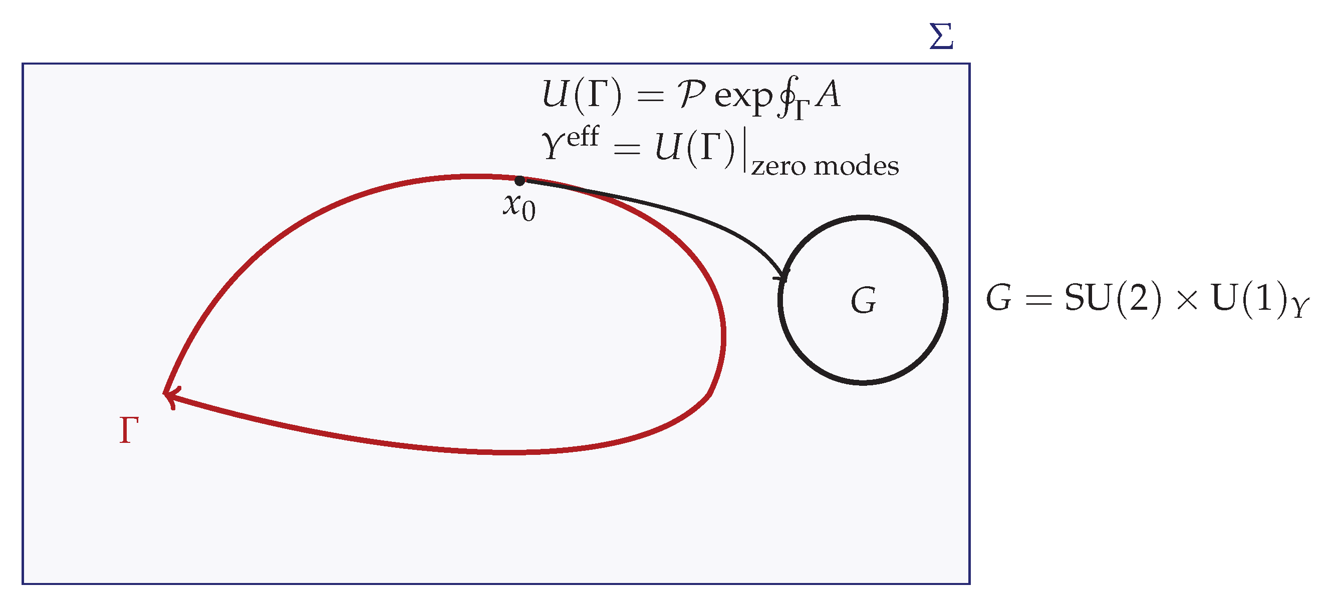
Figure 1. Holonomy on a stabilized spatial leaf $\mathsf{\Sigma }$. The blue rectangle represents the leaf with induced Riemannian metric. A closed loop $\mathsf{\Gamma }$ (red) is traced on the leaf, starting and ending at the basepoint $x_0$. Parallel transport of the internal fiber along $\mathsf{\Gamma }$ is encoded by the path–ordered exponential $U\left(\mathsf{\Gamma }\right)=\mathcal{P}exp{\oint }_{\mathsf{\Gamma }}A$, where A is the $\mathrm{SU}\left(2\right)\times \mathrm{U}{\left(1\right)}_Y$ connection derived from chronon geometry. The fiber sketch on the right indicates the electroweak gauge group $G=\mathrm{SU}\left(2\right)\times \mathrm{U}{\left(1\right)}_Y$ into which the holonomy takes values. When this holonomy acts on fermionic zero modes, its projection defines an effective Yukawa coupling $Y^{\mathrm{eff}}$, which encodes how the chronon–induced gauge structure transmits mass and mixing information to matter fields. Intuitively put, carrying the internal triad once around $\mathsf{\Gamma }$ rotates it by $U\left(\mathsf{\Gamma }\right)$, and the residue of this rotation in the zero–mode sector is the emergent Yukawa interaction.

Figure 1. Holonomy on a stabilized spatial leaf $\mathsf{\Sigma }$. The blue rectangle represents the leaf with induced Riemannian metric. A closed loop $\mathsf{\Gamma }$ (red) is traced on the leaf, starting and ending at the basepoint $x_0$. Parallel transport of the internal fiber along $\mathsf{\Gamma }$ is encoded by the path–ordered exponential $U\left(\mathsf{\Gamma }\right)=\mathcal{P}exp{\oint }_{\mathsf{\Gamma }}A$, where A is the $\mathrm{SU}\left(2\right)\times \mathrm{U}{\left(1\right)}_Y$ connection derived from chronon geometry. The fiber sketch on the right indicates the electroweak gauge group $G=\mathrm{SU}\left(2\right)\times \mathrm{U}{\left(1\right)}_Y$ into which the holonomy takes values. When this holonomy acts on fermionic zero modes, its projection defines an effective Yukawa coupling $Y^{\mathrm{eff}}$, which encodes how the chronon–induced gauge structure transmits mass and mixing information to matter fields. Intuitively put, carrying the internal triad once around $\mathsf{\Gamma }$ rotates it by $U\left(\mathsf{\Gamma }\right)$, and the residue of this rotation in the zero–mode sector is the emergent Yukawa interaction.

2. Preliminaries: Chronon Geometry and Paper I Summary

2.1. Chronon–Induced Foliation and Emergent Metric

Chronon field and normalization.

We assume a smooth, future–directed timelike chronon field

$${\mathsf{\Phi }}^{\mu }\in \mathsf{\Gamma }\left(T\mathcal{U}\right),{\mathsf{\Phi }}^{\mu }{\mathsf{\Phi }}_{\mu }=-1,$$

(4)

defined on an open spacetime domain $\mathcal{U}$. Throughout, indices are raised/lowered with a Lorentzian metric $g_{\mu \nu }$ that is emergent and functionally dependent on $\mathsf{\Phi }$ (Paper I), written $g_{\mu \nu }\equiv g_{\mu \nu }\left[\mathsf{\Phi }\right]$. We work in signature $(-,+,+,+)$ and adopt standard GR conventions for curvature and covariant variation [79].

Intrinsic time and leaves.

Integral curves of $\mathsf{\Phi }$ define a flow ${\phi }_{\tau }:\mathcal{U}\to \mathcal{U}$ with parameter $\tau$ fixed by ${\mathsf{\Phi }}^{\mu }{\nabla }_{\mu }\tau =1$. Leaves are level sets

$${\mathsf{\Sigma }}_{\tau }:=\{x\in \mathcal{U}:\tau \left(x\right)=\mathrm{const}\}.$$

(5)

We say the domain is stabilized if: (i) $\mathsf{\Phi }$ is strictly timelike and smooth with bounded derivatives, (ii) the leaves form a smooth foliation, and (iii) the field equations are hyperbolic with respect to $\tau$ (Paper I). Frobenius’ theorem implies that the foliation is equivalent to vanishing twist

$${\omega }_{\mu \nu }:=h_{\mu }{‌}^{\alpha }{h}_{\nu }{‌}^{\beta }{\nabla }_{[\alpha }{\mathsf{\Phi }}_{\beta ]}=0,$$

(6)

where $h_{\mu \nu }$ is the spatial projector below [79].

Projectors, spatial geometry, and kinematics.

Let

$$h_{\mu \nu }:=g_{\mu \nu }+{\mathsf{\Phi }}_{\mu }{\mathsf{\Phi }}_{\nu },h_{\mu }{‌}^{\nu }:={\delta }_{\mu }{‌}^{\nu }+{\mathsf{\Phi }}_{\mu }{\mathsf{\Phi }}^{\nu },$$

(7)

be the orthogonal projector onto $T{\mathsf{\Sigma }}_{\tau }$. The induced Riemannian metric on ${\mathsf{\Sigma }}_{\tau }$ is

$$h_{ij}={\iota }^{*}{g}_{\mu \nu },\mathrm{d}{\mathrm{vol}}_h=\sqrt{h}{\mathrm{d}}^{3}x,$$

(8)

with $\iota :{\mathsf{\Sigma }}_{\tau }\hookrightarrow \mathcal{U}$ the inclusion and $h=det\left(h_{ij}\right)$. We write the standard kinematic decomposition

$${\nabla }_{\mu }{\mathsf{\Phi }}_{\nu }={\mathsf{\Phi }}_{\mu }{a}_{\nu }+{\sigma }_{\mu \nu }+\frac{1}{3}\theta h_{\mu \nu }+{\omega }_{\mu \nu },$$

(9)

where all tensors on the right are spatial (h–orthogonal to $\mathsf{\Phi }$):

$$\begin{array}{cc}\hfill a_{\mu }& :={\mathsf{\Phi }}^{\alpha }{\nabla }_{\alpha }{\mathsf{\Phi }}_{\mu }\left(\mathrm{acceleration}\right),\hfill \end{array}$$

(10)

$$\begin{array}{cc}\hfill \theta & :={\nabla }_{\mu }{\mathsf{\Phi }}^{\mu }\left(\mathrm{expansion}\right),\hfill \end{array}$$

(11)

$$\begin{array}{cc}\hfill {\sigma }_{\mu \nu }& :=h_{(\mu }{‌}^{\alpha }{h}_{\nu )}{‌}^{\beta }\left({\nabla }_{\alpha }{\mathsf{\Phi }}_{\beta }-\frac{1}{3}\theta h_{\alpha \beta }\right)\left(\mathrm{shear}\right),\hfill \end{array}$$

(12)

$$\begin{array}{cc}\hfill {\omega }_{\mu \nu }& :=h_{[\mu }{‌}^{\alpha }{h}_{\nu ]}{‌}^{\beta }{\nabla }_{\alpha }{\mathsf{\Phi }}_{\beta }\left(\mathrm{twist}\right).\hfill \end{array}$$

(13)

This is the usual $1+3$ covariant split (Raychaudhuri/Ehlers–Ellis) [23,24,62]. The extrinsic curvature of ${\mathsf{\Sigma }}_{\tau }$ is $K_{\mu \nu }:=h_{\mu }{‌}^{\alpha }{h}_{\nu }{‌}^{\beta }{\nabla }_{\alpha }{\mathsf{\Phi }}_{\beta }={\sigma }_{\mu \nu }+\frac{1}{3}\theta h_{\mu \nu }$ (hence $K_{\left[\mu \nu \right]}={\omega }_{\mu \nu }$); ADM language will be used as needed [4].

Emergent metric and $\mathsf{\Phi }$–adapted frames.

A local orthonormal frame $(e_0,e_a)$ adapted to the foliation satisfies $e_0=\mathsf{\Phi }$, $g(e_0,e_0)=-1$, $g(e_a,e_b)={\delta }_{ab}$. Spatial objects are computed with the Levi–Civita connection $D_i$ of $h_{ij}$. In these frames, all leafwise integrals and norms are defined with $h_{ij}$ and $\mathrm{d}{\mathrm{vol}}_h$ (cf. standard GR/ADM formalisms [4,79]).

2.2. Local mass density and solitonic matter

Stress tensor and local mass density.

Let $T_{\mu \nu }$ be the covariant stress tensor of CFT on $(\mathcal{U},g[\mathsf{\Phi }\left]\right)$, obtained by variation of the action with respect to $g_{\mu \nu }$ (Paper I, Appendix A) [44]. On any stabilized domain we impose diffeomorphism invariance ${\nabla }_{\mu }{T}^{\mu \nu }=0$ and quasi–stationarity of the chronon sector along the flow. The local mass/energy density measured by the chronon observer is

$$\rho \left(x\right):=T_{\mu \nu }\left(x\right){\mathsf{\Phi }}^{\mu }\left(x\right){\mathsf{\Phi }}^{\nu }\left(x\right).$$

(14)

Under the induced dominant energy condition (DEC) on leaves, $T_{\mu \nu }{v}^{\mu }{w}^{\nu }\ge 0$ for all future–directed causal $v,w$, positivity is immediate:

$$\rho \left(x\right)=T_{\mu \nu }{\mathsf{\Phi }}^{\mu }{\mathsf{\Phi }}^{\nu }\ge 0,$$

(15)

in line with standard energy conditions [33].

Conserved energy current and leafwise mass.

Define the energy current $J^{\mu }:=T^{\mu \nu }{\mathsf{\Phi }}_{\nu }$. Using ${\nabla }_{\mu }{T}^{\mu \nu }=0$ and the flow invariance of the Lagrangian density along $\mathsf{\Phi }$, one obtains

$${\nabla }_{\mu }{J}^{\mu }=0.$$

(16)

Integrating (16) over a spacetime slab bounded by two leaves and applying the divergence theorem yields leafwise conservation of the total mass

$$\mathsf{M}\left[{\mathsf{\Sigma }}_{\tau }\right]:={\int }_{{\mathsf{\Sigma }}_{\tau }}\rho \mathrm{d}{\mathrm{vol}}_h,\mathsf{M}\left[{\mathsf{\Sigma }}_{{\tau }_2}\right]=\mathsf{M}\left[{\mathsf{\Sigma }}_{{\tau }_1}\right],$$

(17)

for finite–energy configurations (Paper I, Theorem 4.2); the Noether interpretation of stress–tensor conservation follows standard GR/QFT treatments [79].

Topological sectors and solitons.

Compactifying a leaf to $S^3$ by adding the point at spatial infinity (finite–energy boundary conditions), the chronon field (or an associated unit–norm order parameter) defines a map $S^3\to S^3$ with degree

$$w\in {\pi }_3\left(S^3\right)\cong \mathbb{Z}.$$

(18)

Configuration space decomposes as $\mathcal{C}={⨆}_{w\in \mathbb{Z}}{\mathcal{C}}_w$. Let $E\left[\mathsf{\Phi }\right]:={\int }_{{\mathsf{\Sigma }}_{\tau }}\rho \mathrm{d}{\mathrm{vol}}_h$ be the energy functional on a leaf. Under the coercivity and regularity assumptions of Paper I Appendix M) [44], the direct method in the calculus of variations yields:

Existence (Paper I, Appendix M [44]) In $w=1$ there exists a smooth, finite–energy minimizer ${\mathsf{\Phi }}_{★}\in {\mathcal{C}}_1$ (unique up to symmetries under suitable hypotheses). Its energy $M_{w=1}:=E\left[{\mathsf{\Phi }}_{★}\right]$ defines the rest mass of the single–particle excitation. The homotopy and Skyrme–type soliton background are standard [32,51,66].

Spin–statistics via FR/Berry.

Let $M_1$ be the one–soliton moduli space and $C\left(2\right)$ the two–soliton exchange space (configurations of two well–separated $w=1$ solitons modulo translations and overall rotations). Paper I proves

$${\pi }_1\left(M_1\right)\cong {\mathbb{Z}}_2,{\pi }_1\left(C\left(2\right)\right)\cong {\mathbb{Z}}_2.$$

(19)

Quantization proceeds on a Hilbert bundle over $M_1$ with Berry connection. A $2\pi$ spatial rotation and the exchange loop represent the nontrivial element of ${\mathbb{Z}}_2$ and act as $-1$ on the wavefunctional, implying spin–$\frac{1}{2}$ and Fermi–Dirac statistics for the $w=1$ soliton (Finkelstein–Rubinstein mechanism), with the geometric phase furnished by the Berry connection [10,27]. Moreover, Paper I establishes a bundle–matching result: the Berry ${\mathbb{Z}}_2$ holonomy equals the pullback of the emergent spacetime Abelian connection restricted to the soliton configuration bundle (cf. holonomy/Wilson–loop language [2,86]).

Emergent $\mathrm{U}\left(1\right)$ gauge sector.

Parallel transport of $\mathsf{\Phi }$ along leaf loops defines a phase $\theta$ and a one–form $A:=\mathrm{d}\theta$ whose curvature $F=\mathrm{d}A$ is gauge invariant on stabilized domains. The effective action contains

$$S_{\mathrm{EM}}=-{\displaystyle \frac{{\kappa }_A}{4}}{\int }_{\mathcal{U}}\sqrt{-g}{F}_{\mu \nu }{F}^{\mu \nu }{\mathrm{d}}^{4}x,{\kappa }_A>0,$$

(20)

which, after canonical normalization $A_{\mu }^{\mathrm{can}}=\sqrt{{\kappa }_A}{A}_{\mu }$, reproduces Maxwell dynamics on $(\mathcal{U},g[\mathsf{\Phi }\left]\right)$. Solitons couple minimally with bare topological charge $q_0$, so the observed electric charge is

$$e={\displaystyle \frac{q_0}{\sqrt{{\kappa }_A}}}.$$

(21)

Gauge redundancy forbids a Proca term, hence the photon is exactly massless to two derivatives; Ward/Takahashi identities protect $m_{\gamma }=0$ to all orders in the gauge–invariant effective theory [72,80,85]. The Chronon Equivalence Principle introduced in Paper I identifies the soliton rest energy as the static profile energy plus quadratic contributions from internal zero modes, providing the mass mechanism for charged particle excitations, while gauge bosons associated with unbroken $\mathrm{U}\left(1\right)$ remain massless (Paper I).

The results above constitute the geometric and variational backbone on which the non–Abelian electroweak construction of the present paper is built.

3. Internal Fiber Geometry and Principal Non-Abelian Bundle

3.1. Compact Internal Symmetry from Chronon Fiber

We now extend the Abelian holonomy construction of Paper I to the non-Abelian case. The chronon field ${\mathsf{\Phi }}^{\mu }$ defines a stabilized foliation $\left\{{\mathsf{\Sigma }}_{\tau }\right\}$ with induced spatial metric $h_{ij}$ and covariant derivative $D_i$. Parallel transport of $\mathsf{\Phi }$ on ${\mathsf{\Sigma }}_{\tau }$ acts on its internal transverse space, which is naturally three-dimensional and compactifiable to $S^3$ (cf. standard target-space models and $S^3\simeq SU\left(2\right)$) [54]. This motivates the following definition of the internal configuration space:

$$\mathcal{C}:=\{\mathsf{\Phi }:{\mathsf{\Sigma }}_{\tau }\to S^3\subset {\mathbb{R}}^4\},$$

endowed with the $L^2$ topology on derivatives $D_i\mathsf{\Phi }$. The residual symmetries are given by smooth orthonormal rotations of the internal $S^3$, i.e. the group $\mathrm{SO}\left(4\right)$ acting on target space. We focus on compact subgroups acting freely on fibers.

Assumption A1 

(Compactness and regularity). The internal chronon fiber admits a compact subgroup $K\cong \mathrm{SU}\left(2\right)‌$ with smooth action and global trivializations on a good cover $\left\{U_{\alpha }\right\}$ of $\mathcal{M}$. Equivalently, there exists a $\mathrm{SU}\left(2\right)‌$ action

$$\rho :\mathrm{SU}\left(2\right)‌\times \mathcal{C}\to \mathcal{C}$$

that is free, proper, and smooth, such that transition functions $g_{\alpha \beta }:U_{\alpha }\cap U_{\beta }\to \mathrm{SU}\left(2\right)‌$ are well-defined and satisfy the cocycle condition [34,38,68].

The freeness of the action ensures that fibers carry no residual stabilizers, while compactness guarantees finite holonomy. The requirement of a good cover implies that $\mathcal{C}$ admits local trivializations compatible with the $\mathrm{SU}\left(2\right)‌$ action [34,68].

Theorem 4 

(Emergent principal $\mathrm{SU}\left(2\right)$ bundle and connection). Under ?? 1, there exists a principal $\mathrm{SU}\left(2\right)‌$ bundle $P\to \mathcal{M}$ and a connection $\mathcal{A}\in {\mathsf{\Omega }}^1(P,\mathfrak{su}\left(2\right))$ induced by chronon holonomy on leaves $\left\{{\mathsf{\Sigma }}_{\tau }\right\}$. Its curvature $\mathcal{F}=d\mathcal{A}+\mathcal{A}\wedge \mathcal{A}$ coincides with the parallel-transport holonomy two-form of the internal fiber [2,22,38].

Idea. 

Cover $\mathcal{M}$ by $\left\{U_{\alpha }\right\}$ on which the internal fiber trivializes smoothly with respect to $\mathrm{SU}\left(2\right)‌$. For each overlap $U_{\alpha }\cap U_{\beta }$, define a transition function $g_{\alpha \beta }:U_{\alpha }\cap U_{\beta }\to \mathrm{SU}\left(2\right)‌$ via chronon holonomy computed along paths confined to ${\mathsf{\Sigma }}_{\tau }$. Freeness of the $\mathrm{SU}\left(2\right)‌$ action ensures uniqueness of $g_{\alpha \beta }$, and parallel transport consistency implies the cocycle condition $g_{\alpha \beta }{g}_{\beta \gamma }{g}_{\gamma \alpha }=e$; hence $\left\{g_{\alpha \beta }\right\}$ defines a principal $\mathrm{SU}\left(2\right)‌$ bundle $P\to \mathcal{M}$ [34,68].

The local connection one-forms ${\mathcal{A}}_{\alpha }\in {\mathsf{\Omega }}^1(U_{\alpha },\mathfrak{su}\left(2\right))$ are defined by pullback of the leafwise parallel-transport operator of $\mathsf{\Phi }$. On overlaps, ${\mathcal{A}}_{\beta }=g_{\alpha \beta }^{-1}{\mathcal{A}}_{\alpha }{g}_{\alpha \beta }+g_{\alpha \beta }^{-1}\mathrm{d}{g}_{\alpha \beta }$, so they patch to a global $\mathrm{SU}\left(2\right)‌$ connection $\mathcal{A}\in {\mathsf{\Omega }}^1(P,\mathfrak{su}\left(2\right))$ [38]. By the Ambrose–Singer theorem, the curvature $\mathcal{F}$ computed from $\mathcal{A}$ generates the holonomy and thus agrees with the holonomy two-form of chronon parallel transport, providing the non-Abelian generalization of the Abelian result $F=\mathrm{d}A$ from Paper I [2,38]. □

Role of the unit–norm constraint.

Throughout we impose ${\mathsf{\Phi }}^{\mu }{\mathsf{\Phi }}_{\mu }=-1$ on stabilized domains (Paper I). This ensures that the orthogonal projector ${\Pi }^{\mu }{‌}_{\nu }={\delta }^{\mu }{‌}_{\nu }+{\mathsf{\Phi }}^{\mu }{\mathsf{\Phi }}_{\nu }$ is idempotent and annihilates $\mathsf{\Phi }$, so that $T\mathcal{M}=\mathrm{span}\left\{\mathsf{\Phi }\right\}\oplus {\mathsf{\Phi }}^{\perp }$ and the induced leaf metric $h_{\mu \nu }=g_{\mu \nu }\left[\mathsf{\Phi }\right]+{\mathsf{\Phi }}_{\mu }{\mathsf{\Phi }}_{\nu }$ are well defined. Parallel transport restricted to ${\mathsf{\Phi }}^{\perp }$ preserves h and thus has compact structure group $\mathrm{SO}\left(3\right)$, with double cover $\mathrm{SU}\left(2\right)$, which underlies ?? 1 and Theorem 4 [54,56,79]. In the mass generation sector, the unit–norm defines the baseline about which amplitude fluctuations H (composite realization) and compact phase variables (Stückelberg realization) are separated; without this normalization, phase–amplitude mixing obstructs a clean gauge–invariant mass term and the holonomy need not remain compact.

Remarks.

• The internal fiber thus carries a canonical non-Abelian structure group $\mathrm{SU}\left(2\right)‌$, generalizing the emergent $U\left(1\right)$ bundle of Paper I [38,68].
• The curvature $\mathcal{F}$ encodes parallel-transport anomalies in the chronon geometry; in the next section this becomes the field strength of an emergent Yang–Mills sector [2,38].
• This construction is functorial: any stabilized domain $(U,g[\mathsf{\Phi }\left]\right)$ admits the associated bundle ${P|}_U$, unique up to gauge equivalence [34].

4. Emergent Yang–Mills Action on $g\left[\mathsf{\Phi }\right]$

Having established the existence of a principal $\mathrm{SU}\left(2\right)‌$ bundle $P\to \mathcal{M}$ with connection $\mathcal{A}$ induced by chronon holonomy (Theorem 4), we now derive the associated Yang–Mills dynamics on the emergent background metric $g_{\mu \nu }\left[\mathsf{\Phi }\right]$.

4.1. Gauge Transformations and Curvature

Let $A_{\mu }=A_{\mu }^a{T}^a$ denote the local connection one-form on $\mathcal{M}$, with ${\left\{T^a\right\}}_{a=1}^3$ a basis of $\mathfrak{su}\left(2\right)$ normalized by $\mathrm{tr}\left(T^a{T}^b\right)=\frac{1}{2}{\delta }^{ab}$. The curvature two-form is

$$F_{\mu \nu }={\partial }_{\mu }{A}_{\nu }-{\partial }_{\nu }{A}_{\mu }+[A_{\mu },A_{\nu }]=F_{\mu \nu }^a{T}^a,$$

(22)

where $F_{\mu \nu }^a={\partial }_{\mu }{A}_{\nu }^a-{\partial }_{\nu }{A}_{\mu }^a+f^{abc}{A}_{\mu }^b{A}_{\nu }^c$ and $f^{abc}$ are the structure constants of $\mathfrak{su}\left(2\right)$ [88].

Under a gauge transformation $g:\mathcal{M}\to \mathrm{SU}\left(2\right)‌$, the connection transforms as

$$A_{\mu }\mapsto g^{-1}{A}_{\mu }g+g^{-1}{\partial }_{\mu }g,$$

(23)

while the curvature transforms covariantly:

$$F_{\mu \nu }\mapsto g^{-1}{F}_{\mu \nu }g,$$

(24)

consistent with standard bundle connections [38,54].

Theorem 5 

(Yang–Mills sector from holonomy). On a stabilized domain $(\mathcal{M},g[\mathsf{\Phi }\left]\right)$, the functional

$$S_{\mathrm{YM}}[A;\mathsf{\Phi }]=-{\displaystyle \frac{1}{2g^2}}{\int }_{\mathcal{M}}\mathrm{tr}\left(F_{\mu \nu }{F}^{\mu \nu }\right)\sqrt{-g\left[\mathsf{\Phi }\right]}{\mathrm{d}}^{4}x$$

(25)

is invariant under the holonomy-induced $\mathrm{SU}\left(2\right)‌$ gauge group. Variation with respect to $A_{\mu }$ yields the Yang–Mills field equations on the emergent metric:

$${\nabla }_{\mu }{F}^{\mu \nu }+[A_{\mu },F^{\mu \nu }]=0,$$

(26)

where ∇ is the Levi–Civita derivative of $g\left[\mathsf{\Phi }\right]$ acting on tensor indices.

Proof sketch. 

Gauge invariance follows from cyclicity of the trace and covariance of $F_{\mu \nu }$ [88]. Varying (25) with respect to $A_{\mu }$ and integrating by parts, using the antisymmetry of $F_{\mu \nu }$ and compact support of variations, yields $\delta S_{\mathrm{YM}}=\frac{1}{g^2}\int \mathrm{tr}\left(({\nabla }_{\mu }{F}^{\mu \nu }+[A_{\mu },F^{\mu \nu }])\delta A_{\nu }\right)\sqrt{-g}{\mathrm{d}}^{4}x,$ so the Euler–Lagrange equations are as stated [60]. □

4.2. Coupling to Solitonic Matter

In Chronon Field Theory, solitons of charge $w=1$ (Paper I) serve as particle excitations with spin and statistics inherited from the topology of the moduli space. The emergent $\mathrm{SU}\left(2\right)‌$ symmetry acts on internal zero modes of these solitons, realizing an isospin representation, in analogy with Skyrmions carrying $SU\left(2\right)$ quantum numbers [51,66].

Let $\mathsf{\Psi }$ denote a collective-coordinate wavefunctional on the soliton moduli space ${\mathcal{M}}_1$. The $\mathrm{SU}\left(2\right)‌$ action lifts to $\mathsf{\Psi }$ as an isospin representation $\rho :\mathrm{SU}\left(2\right)‌\to \mathrm{End}\left(V\right)$, with Lie algebra action $\rho \left(T^a\right)=\frac{i}{2}{\tau }^a$ in the fundamental case. Minimal coupling is then introduced by replacing ordinary derivatives with covariant ones:

$$D_{\mu }\mathsf{\Psi }={\partial }_{\mu }\mathsf{\Psi }+\rho \left(A_{\mu }\right)\mathsf{\Psi },$$

(27)

in direct analogy with standard non-Abelian gauge coupling [60,88]. Equivalently, the soliton Hamiltonian is deformed by

$$H\mapsto H\left(A\right)=H\left(0\right){|}_{\partial \to D},$$

(28)

ensuring gauge invariance under the holonomy-induced $\mathrm{SU}\left(2\right)‌$.

Remarks.

• This construction promotes solitons to carriers of isospin, with multiplet structure determined by the representation $\rho$ of $\mathrm{SU}\left(2\right)‌$.
• Coupling constants are set by the holonomy stiffness ${\kappa }_2$ (Theorem 5), fixing the normalization of the gauge field kinetic term and its interaction strength.
• The framework parallels the Abelian case of Paper I but naturally accommodates non-Abelian charge sectors and multiplets, as required for electroweak-like dynamics.

Anomaly considerations.

Minimal coupling of solitonic matter to the emergent $\mathrm{SU}\left(2\right)‌\times \mathrm{U}\left(1\right){‌}_Y$ connection introduces the usual consistency requirements of gauge anomalies [1,9]. In the sectors analyzed here, the effective soliton spectrum couples vectorially to $\mathrm{SU}\left(2\right)‌$ and carries anomaly-free hypercharge assignments, so that the $\mathrm{SU}{\left(2\right)}^2\mathrm{U}\left(1\right)$ and $\mathrm{U}{\left(1\right)}^3$ triangle anomalies cancel. Global $\mathrm{SU}\left(2\right)$ anomalies (Witten’s ${\pi }_4\left(\mathrm{SU}\left(2\right)\right)={\mathbb{Z}}_2$ obstruction) are likewise avoided since only integer isospin representations arise in the quantization of solitonic moduli [87]. A systematic classification of anomaly-free soliton representations is left for future work, but the consistency of the constructions considered here is preserved.

5. Electroweak-Like Mixing and Photon Masslessness

We now extend the pure $\mathrm{SU}\left(2\right)‌$ sector to the product group $\mathrm{SU}\left(2\right)‌\times \mathrm{U}\left(1\right){‌}_Y$, where the additional $\mathrm{U}\left(1\right){‌}_Y$ factor is induced by Abelian chronon holonomy as in Paper I. The combined gauge structure mirrors the electroweak group of the Standard Model, and its internal alignment leads to an unbroken $\mathrm{U}\left(1\right){‌}_{\mathrm{em}}$ symmetry with a massless photon [29,64,81].

5.1. Constructing $\mathrm{SU}\left(2\right)‌\times \mathrm{U}\left(1\right)‌$ and mixing

Let $A_{\mu }=A_{\mu }^a{T}^a$ denote the $\mathrm{SU}\left(2\right)‌$ gauge potential with curvature $F_{\mu \nu }$ as in Section 4, and let $B_{\mu }$ denote the $\mathrm{U}\left(1\right){‌}_Y$ connection one-form with curvature

$$F_{\mu \nu }^Y={\partial }_{\mu }{B}_{\nu }-{\partial }_{\nu }{B}_{\mu }.$$

(29)

The full gauge group is the direct product

$$G_{\mathrm{EW}}=\mathrm{SU}\left(2\right)‌\times \mathrm{U}\left(1\right){‌}_Y,$$

(30)

with generators ${\left\{T^a\right\}}_{a=1}^3$ for $\mathrm{SU}\left(2\right)‌$ and Y for $\mathrm{U}\left(1\right){‌}_Y$, obeying $[T^a,T^b]=i{f}^{abc}{T}^c$, $[T^a,Y]=0$ [88].

The gauge kinetic action is

$$S_{\mathrm{gauge}}=-{\displaystyle \frac{1}{2g^2}}\int \mathrm{tr}\left(F_{\mu \nu }{F}^{\mu \nu }\right)\sqrt{-g\left[\mathsf{\Phi }\right]}{\mathrm{d}}^{4}x-{\displaystyle \frac{1}{4g^{\prime 2}}}\int F_{\mu \nu }^Y{F}^{Y\mu \nu }\sqrt{-g\left[\mathsf{\Phi }\right]}{\mathrm{d}}^{4}x,$$

(31)

with independent couplings $g,g^{\prime }>0$ [60].

Coupling to solitonic matter proceeds by assigning to each soliton multiplet a representation $\rho$ of $\mathrm{SU}\left(2\right)‌$ and a hypercharge $y\in \mathbb{Z}$, so that the covariant derivative is

$$D_{\mu }={\partial }_{\mu }+\rho \left(A_{\mu }\right)+iy{B}_{\mu }.$$

(32)

Proposition 2 

(Residual $\mathrm{U}\left(1\right)‌$ and photon). Consider the subgroup of $G_{\mathrm{EW}}$ generated by

$$Q=T^3+Y.$$

(33)

Then for a suitable mixing angle ${\theta }_W$ defined by $tan{\theta }_W=g^{\prime }/g$, the corresponding gauge boson

$$A_{\mu }=sin{\theta }_W{A}_{\mu }^3+cos{\theta }_W{B}_{\mu }$$

(34)

remains exactly massless, generating an unbroken $\mathrm{U}\left(1\right){‌}_{\mathrm{em}}$ symmetry [64,81]. The orthogonal combinations

$$W_{\mu }^{\pm }=\frac{1}{\sqrt{2}}(A_{\mu }^1\mp i{A}_{\mu }^2),Z_{\mu }=cos{\theta }_W{A}_{\mu }^3-sin{\theta }_W{B}_{\mu },$$

(35)

may acquire masses through chronon-induced symmetry breaking (CISB), while the photon $A_{\mu }$ is protected by gauge invariance.

Idea. 

The construction of the unbroken generator Q follows the standard Cartan embedding: the diagonal generator $T^3$ of $\mathrm{SU}\left(2\right)‌$ commutes with the $\mathrm{U}\left(1\right){‌}_Y$ generator Y, and their linear combination $Q=T^3+Y$ defines a maximal torus subgroup $\mathrm{U}\left(1\right){‌}_{\mathrm{em}}\subset G_{\mathrm{EW}}$. By the structure of CISB (chronon alignment of the internal fiber), gauge bosons acquire a mass matrix with one null eigenvalue corresponding to Q [81]. Explicitly, in the $(A_{\mu }^3,B_{\mu })$ basis, the quadratic form is proportional to

$$M^2\propto \left(\begin{array}{cc}{g}^2& -g{g}^{\prime }\\ -g{g}^{\prime }& g^{\prime 2}\end{array}\right),$$

which has determinant zero and rank one. Its zero eigenvector is $sin{\theta }_W{A}_{\mu }^3+cos{\theta }_W{B}_{\mu }$, proving that $A_{\mu }$ is exactly massless. Ward identities inherited from gauge invariance guarantee that this remains true to all orders [60]. □

Remarks.

• The unbroken $\mathrm{U}\left(1\right){‌}_{\mathrm{em}}$ is intrinsic to the bundle structure and does not rely on a fundamental scalar Higgs. Its generator Q is uniquely fixed by the chronon-induced alignment.
• The relation $m_W=m_{Z}cos{\theta }_W$ emerges at quadratic order in the CISB effective action, ensuring custodial consistency [29,81].
• Solitons charged under $\mathrm{U}\left(1\right){‌}_{\mathrm{em}}$ inherit electric charges $q=t^3+y$, where $t^3$ is the $\mathrm{SU}\left(2\right)‌$ weight and y the hypercharge.

6. Vector Mass Generation Without a Fundamental Higgs

We now describe how gauge boson masses arise in Chronon Field Theory (CFT) without introducing a fundamental Higgs scalar. The mechanism is geometric: internal phases of the chronon fiber play the role of Stückelberg fields, while amplitude fluctuations of $\mathsf{\Phi }$ supply an effective radial mode. Both constructions preserve gauge invariance and ensure that one linear combination of gauge bosons remains massless, echoing classic non-linear realizations of symmetry breaking [12,69].

6.1. Stückelberg-Like Realization

Let ${\pi }^a\left(x\right)$ ($a=1,2,3$) denote internal phase fields parameterizing fluctuations of the chronon fiber transverse to the stabilized alignment. Define the group-valued field

$$\mathsf{\Sigma }\left(x\right)=exp\left[{\displaystyle \frac{i}{v}}{\pi }^a\left(x\right)T^a\right]\in \mathrm{SU}\left(2\right)‌,$$

(36)

where v is a chronon-induced scale (analogous to the electroweak scale in the SM). The covariant derivative acts as

$$D_{\mu }\mathsf{\Sigma }={\partial }_{\mu }\mathsf{\Sigma }+A_{\mu }\mathsf{\Sigma }-\mathsf{\Sigma }{B}_{\mu }Y,$$

(37)

with $A_{\mu }=A_{\mu }^a{T}^a$ the $\mathrm{SU}\left(2\right)‌$ connection and $B_{\mu }$ the $\mathrm{U}\left(1\right){‌}_Y$ field. The gauge-invariant effective Lagrangian is

$${\mathcal{L}}_{\mathrm{St}}={\displaystyle \frac{v^2}{4}}\mathrm{tr}\left({\left(D_{\mu }\mathsf{\Sigma }\right)}^{†}{D}^{\mu }\mathsf{\Sigma }\right).$$

(38)

In unitary gauge $\mathsf{\Sigma }\equiv 1$, the phases ${\pi }^a$ are eaten and (38) reduces to explicit mass terms for gauge bosons, while preserving $\mathrm{U}\left(1\right){‌}_{\mathrm{em}}$ invariance as identified in Proposition 2 [64,81].

6.2. Composite Amplitude Mode of $\mathsf{\Phi }$

In addition to phase fluctuations, the chronon norm constraint admits a radial (amplitude) fluctuation $H\left(x\right)$, arising from restoring terms in the action (e.g. the Lagrange multiplier $\lambda$ in Paper I). This field behaves as a composite scalar excitation of $\mathsf{\Phi }$. An effective non-linear sigma model takes the form

$${\mathcal{L}}_{\mathrm{amp}}={\displaystyle \frac{1}{2}}\left({\partial }_{\mu }H\right)\left({\partial }^{\mu }H\right)-V\left(H\right)+{\displaystyle \frac{{(v+H)}^2}{4}}\mathrm{tr}\left({\left(D_{\mu }\mathsf{\Sigma }\right)}^{†}{D}^{\mu }\mathsf{\Sigma }\right),$$

(39)

with potential $V\left(H\right)$ stabilizing H at $\langle H\rangle =0$. In this realization, the amplitude mode H plays the role of a composite Higgs, ensuring tree-level unitarization of longitudinal vector scattering (cf. §Section 7), as in technicolor and composite Higgs frameworks [70,83].

Proposition 3 

(Mass matrix and eigenstates). In the broken phase induced by Σ, the quadratic gauge-field Lagrangian is

$${\mathcal{L}}_{\mathrm{mass}}={\displaystyle \frac{v^2}{8}}\left[g^2\left({\left(A_{\mu }^1\right)}^2+{\left(A_{\mu }^2\right)}^2\right)+{(g{A}_{\mu }^3-g^{\prime }{B}_{\mu })}^2\right],$$

(40)

where $g,g^{\prime }$ are the canonical couplings. The resulting mass spectrum is:

$$\begin{array}{cc}\hfill m_W& =\frac{1}{2}gv,\hfill \end{array}$$

(41)

$$\begin{array}{cc}\hfill m_Z& =\frac{1}{2}v\sqrt{g^2+g^{\prime 2}},\hfill \end{array}$$

(42)

$$\begin{array}{cc}\hfill m_{\gamma }& =0,\hfill \end{array}$$

(43)

with mass eigenstates

$$\begin{array}{cc}\hfill W_{\mu }^{\pm }& =\frac{1}{\sqrt{2}}(A_{\mu }^1\mp i{A}_{\mu }^2),\hfill \end{array}$$

(44)

$$\begin{array}{cc}\hfill Z_{\mu }& =cos{\theta }_W{A}_{\mu }^3-sin{\theta }_W{B}_{\mu },\hfill \end{array}$$

(45)

$$\begin{array}{cc}\hfill A_{\mu }& =sin{\theta }_W{A}_{\mu }^3+cos{\theta }_W{B}_{\mu },\hfill \end{array}$$

(46)

where $tan{\theta }_W=g^{\prime }/g$. Thus the photon $A_{\mu }$ remains exactly massless, while $W_{\mu }^{\pm }$ and $Z_{\mu }$ acquire masses determined by chronon-sector parameters and the mixing angle ${\theta }_W$ [29,81].

Sketch. 

Expanding ${\mathcal{L}}_{\mathrm{St}}$ to quadratic order in gauge fields yields the mass bilinear. The $(A_{\mu }^1,A_{\mu }^2)$ modes acquire degenerate mass $m_W$. The $(A_{\mu }^3,B_{\mu })$ block has mass matrix

$${\displaystyle \frac{v^2}{4}}\left(\begin{array}{cc}{g}^2& -g{g}^{\prime }\\ -g{g}^{\prime }& g^{\prime 2}\end{array}\right),$$

which has eigenvalues 0 and $\frac{v^2}{4}(g^2+g^{\prime 2})$. The corresponding eigenvectors define $A_{\mu }$ and $Z_{\mu }$, with mixing angle $tan{\theta }_W=g^{\prime }/g$. Gauge invariance of $\mathrm{U}\left(1\right){‌}_{\mathrm{em}}$ ensures the zero eigenvalue persists to all orders [60]. □

Remarks.

• The chronon-induced scale v sets the overall vector mass scale, analogous to the Higgs vacuum expectation value in the SM [81].
• The Stückelberg and amplitude-mode realizations are not mutually exclusive: the phases provide longitudinal degrees of freedom, while the composite $H\left(x\right)$ can unitarize scattering amplitudes [70,83].
• Crucially, no fundamental scalar field is required; all degrees of freedom descend from chronon fiber geometry.

7. Ward Identities, BRST, and Longitudinal Unitarity

Gauge invariance of the holonomy-induced $\mathrm{SU}\left(2\right)‌\times \mathrm{U}\left(1\right){‌}_Y$ sector must be maintained at the quantum level. This requires a consistent gauge-fixing procedure, introduction of Faddeev–Popov ghosts, and demonstration of BRST symmetry [8,25,76]. We then establish that physical amplitudes are gauge-parameter independent (Slavnov–Taylor identities) [67,73], and that longitudinal vector-boson scattering remains unitary at tree level within the validity range of the effective theory [43].

7.1. Gauge Fixing and Ghost Sector

We adopt covariant $R_{\xi }$ gauges on the emergent bundle. For the $\mathrm{SU}\left(2\right)‌$ sector,

$${\mathcal{L}}_{\mathrm{gf}}^{\mathrm{SU}\left(2\right)‌}=-{\displaystyle \frac{1}{2\xi }}{\left({\partial }^{\mu }{A}_{\mu }^a-\xi m_W{\pi }^a\right)}^2,$$

(47)

where ${\pi }^a$ denote the Stückelberg (or would-be Goldstone) fields eaten by the massive vectors. Similarly, for the $\mathrm{U}\left(1\right){‌}_Y$ field $B_{\mu }$ we write

$${\mathcal{L}}_{\mathrm{gf}}^Y=-{\displaystyle \frac{1}{2\xi }}{({\partial }^{\mu }{B}_{\mu }-\xi m_Z{\pi }^Y)}^2.$$

(48)

The corresponding Faddeev–Popov Lagrangian introduces anticommuting ghost fields $c^a,{\overline{c}}^a$ for $\mathrm{SU}\left(2\right)‌$ and $c^Y,{\overline{c}}^Y$ for $\mathrm{U}\left(1\right){‌}_Y$ [25]:

$${\mathcal{L}}_{\mathrm{ghost}}={\overline{c}}^a{\partial }^{\mu }{\left(D_{\mu }c\right)}^a+{\overline{c}}^Y{\partial }^{\mu }{\partial }_{\mu }{c}^Y+\dots ,$$

(49)

with $D_{\mu }c={\partial }_{\mu }c+[A_{\mu },c]$ the covariant derivative in the adjoint.

These terms can be packaged into a nilpotent BRST operator s, defined by

$$\begin{array}{cccc}\hfill s{A}_{\mu }& =D_{\mu }c,\hfill & \hspace{1em}\hspace{1em}\hspace{1em}\hspace{1em}\hspace{1em}\hspace{1em}\hspace{1em}\hfill s{B}_{\mu }& ={\partial }_{\mu }{c}^Y,\hfill \end{array}$$

(50)

$$\begin{array}{cccc}\hfill sc& =-\frac{1}{2}[c,c],\hfill & \hspace{1em}\hspace{1em}\hspace{1em}\hspace{1em}\hspace{1em}\hspace{1em}\hspace{1em}\hfill s{c}^Y& =0,\hfill \end{array}$$

(51)

$$\begin{array}{cccc}\hfill s\overline{c}& ={\displaystyle \frac{1}{\xi }}{\partial }^{\mu }{A}_{\mu },\hfill & \hspace{1em}\hspace{1em}\hspace{1em}\hspace{1em}\hspace{1em}\hspace{1em}\hspace{1em}\hfill s{\overline{c}}^Y& ={\displaystyle \frac{1}{\xi }}{\partial }^{\mu }{B}_{\mu },\hfill \end{array}$$

(52)

extended to matter fields by $s\mathsf{\Psi }=i(c^a{T}^a+c^{Y}Y)\mathsf{\Psi }$. Nilpotency $s^2=0$ follows from the Jacobi identity and the algebra of $G_{\mathrm{EW}}$ [8,76].

Theorem 6 

(Ward/Slavnov–Taylor identities). The emergent non-Abelian sector satisfies the Slavnov–Taylor identities associated to BRST invariance. Consequently, S-matrix elements between physical states are independent of the gauge parameter ξ and respect the underlying $\mathrm{SU}\left(2\right)‌\times \mathrm{U}\left(1\right){‌}_Y$ symmetry [67,73].

Sketch. 

The total gauge-fixed Lagrangian

$${\mathcal{L}}_{\mathrm{tot}}={\mathcal{L}}_{\mathrm{YM}}+{\mathcal{L}}_{\mathrm{mass}}+{\mathcal{L}}_{\mathrm{gf}}+{\mathcal{L}}_{\mathrm{ghost}}$$

is BRST invariant by construction. BRST invariance of the path integral measure implies the generating functional satisfies the Zinn–Justin equation [89], which in turn yields the Slavnov–Taylor identities. These guarantee that variations with respect to $\xi$ vanish on physical amplitudes, completing the argument. □

Theorem 7 

(Tree-level unitarity of longitudinal scattering). In the high-energy limit, scattering amplitudes of longitudinal vector bosons, such as $W_L{W}_L\to W_L{W}_L$ and $W_L{W}_L\to Z_L{Z}_L$, exhibit the required cancellations so that

$$\mathcal{A}\left(E\right)\sim \mathcal{O}\left(E^0\right)\mathrm{as}E\to \infty ,$$

provided the mass-generation sector is realized either via Stückelberg fields or a composite amplitude mode of Φ with appropriately normalized low-energy constants [43].

Strategy. 

By the equivalence theorem [17], the high-energy limit of longitudinal gauge-boson scattering coincides with scattering of the corresponding would-be Goldstone fields ${\pi }^a$. Expanding the effective Lagrangian in partial waves, naive power counting produces $\mathcal{O}\left(E^2\right)$ and $\mathcal{O}\left(E^1\right)$ growth terms. However:

• $\mathcal{O}\left(E^2\right)$ terms cancel between diagrams due to gauge invariance and the precise relation between $m_W$, $m_Z$, and ${\theta }_W$ fixed by the chronon holonomy sector.
• $\mathcal{O}\left(E^1\right)$ terms cancel if the low-energy constants in the Stückelberg realization (or, equivalently, the couplings of the composite amplitude mode H) satisfy $g_{HVV}\simeq 2m_V^2/v$ for $V=W,Z$.

The remaining amplitude is bounded, $\mathcal{A}\left(E\right)\sim \mathcal{O}\left(E^0\right)$, ensuring tree-level partial-wave unitarity up to the cutoff scale ${\mathsf{\Lambda }}_{*}$, set by the onset of new chronon resonances [43]. □

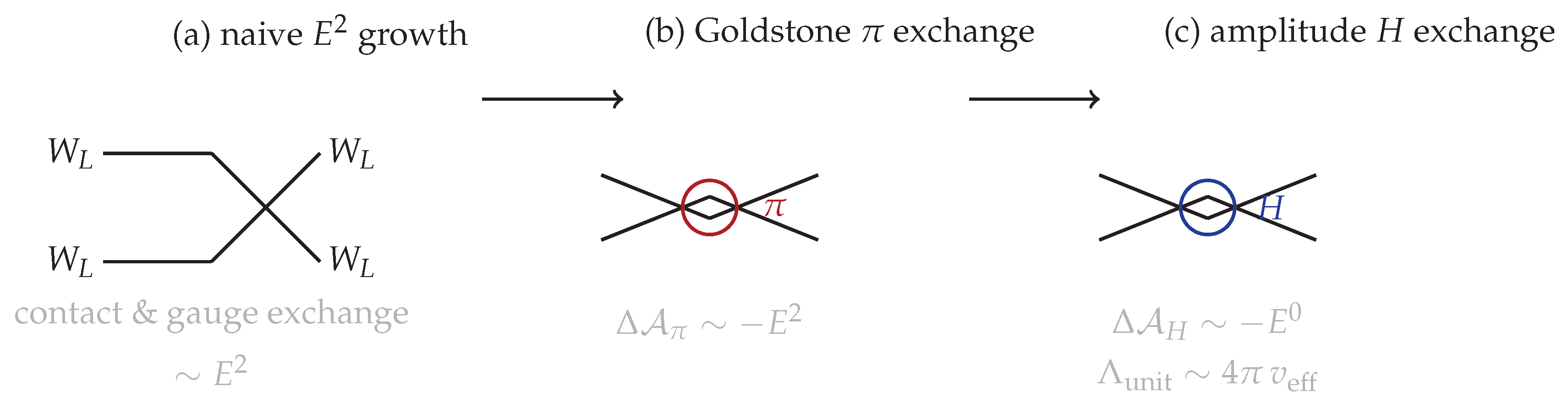
Figure 2. Longitudinal unitarity in $W_L{W}_L$ scattering. Goldstone exchange from $\mathsf{\Sigma }$ cancels the leading $E^2$ growth; amplitude-mode H exchange tames the residual growth, yielding perturbative unitarity up to ${\mathsf{\Lambda }}_{\mathrm{unit}}\sim 4\pi v_{\mathrm{eff}}$.

Figure 2. Longitudinal unitarity in $W_L{W}_L$ scattering. Goldstone exchange from $\mathsf{\Sigma }$ cancels the leading $E^2$ growth; amplitude-mode H exchange tames the residual growth, yielding perturbative unitarity up to ${\mathsf{\Lambda }}_{\mathrm{unit}}\sim 4\pi v_{\mathrm{eff}}$.

Remarks.

• The cancellations that enforce unitarity are not accidental: they follow from the holonomy-induced structure of the mass-generation sector and the custodial relation $m_W=m_{Z}cos{\theta }_W$.
• If the composite amplitude mode H is light, it plays the role of an emergent Higgs-like scalar and unitarizes amplitudes as in the SM. Otherwise, unitarity is maintained only up to ${\mathsf{\Lambda }}_{*}\sim 4\pi v$, beyond which new chronon-sector states must appear.
• BRST symmetry guarantees gauge-parameter independence of these statements, ensuring their robustness within the effective theory.

8. Phenomenology and Constraints

The chronon-induced electroweak sector must be consistent with stringent experimental tests. We summarize the principal phenomenological consequences and constraints.

• Precision electroweak observables. The vector-boson mass relations derived in Proposition 3 yield

  $$m_W=\frac{1}{2}gv,m_Z=\frac{1}{2}v\sqrt{g^2+g^{\prime 2}},{sin}^2{\theta }_W={\displaystyle \frac{g^{\prime 2}}{g^2+g^{\prime 2}}}.$$

  (53)

  The tree-level $\rho$ parameter,

  $$\rho \equiv {\displaystyle \frac{m_W^2}{m_Z^2{cos}^2{\theta }_W}}=1,$$

  (54)

  is protected by the custodial relation enforced by chronon holonomy [65,78]. Radiative corrections and higher-derivative operators can shift $\rho$; present limits require $|\rho -1|\lesssim {10}^{-3}$, constraining higher-order terms in the CFT effective action [57].
  Oblique parameters $(S,T,U)$ encode deviations in gauge-boson self-energies [58,59]. Integrating out chronon fluctuations generates dimension-six operators such as

  $${\displaystyle \frac{c_S}{{\mathsf{\Lambda }}^2}}{H}^{†}{W}_{\mu \nu }{B}^{\mu \nu }H,{\displaystyle \frac{c_T}{{\mathsf{\Lambda }}^2}}{\left(H^{†}{D}_{\mu }H\right)}^2,$$

  with H replaced by the composite amplitude mode. Current bounds, $\left|S\right|,\left|T\right|,\left|U\right|\lesssim 0.1$, translate into constraints on the cutoff scale $\mathsf{\Lambda }$ and the coefficients $c_{S,T,U}$ [7].
• Photon mass bounds. The unbroken generator $Q=T^3+Y$ guarantees an exactly massless photon at all orders. Experimentally, $m_{\gamma }<{10}^{-18}\mathrm{eV}$ provides a sharp test [30,57]: any chronon-sector deformation violating exact $\mathrm{U}\left(1\right){‌}_{\mathrm{em}}$ invariance is excluded at extraordinary precision. Our construction ensures gauge redundancy protects the photon mass to all perturbative orders.
• Triple and quartic gauge couplings. Deviations from Standard Model predictions can arise from higher-derivative operators in the CFT effective action. For instance,

  $$\Delta \mathcal{L}\sim {\displaystyle \frac{1}{{\mathsf{\Lambda }}^2}}\mathrm{tr}\left(\left(D_{\mu }{F}^{\mu \nu }\right)\left(D^{\rho }{F}_{\rho \nu }\right)\right),$$

  (55)

  modifies triple and quartic vertices. LEP and LHC data constrain anomalous couplings at the few-percent level [5,42], implying $\mathsf{\Lambda }\gtrsim \mathrm{TeV}$ for $\mathcal{O}\left(1\right)$ coefficients.
• Birefringence and $\nabla \mathsf{\Phi }$. Residual gradients of the chronon field, $\nabla \mathsf{\Phi }$, generate Lorentz-violating effective operators such as

  $$\Delta {\mathcal{L}}_{\mathrm{LV}}\sim {\displaystyle \frac{1}{{\mathsf{\Lambda }}^2}}\left({\nabla }_{\mu }{\mathsf{\Phi }}_{\nu }\right)F^{\mu \rho }{F}^{\nu }{‌}_{\rho }.$$

  (56)

  These terms induce birefringence and modified dispersion for gauge bosons. Astrophysical observations constrain such effects at the level of ${10}^{-32}$ relative to the photon energy [39,40], placing very strong bounds on the allowed size of $\nabla \mathsf{\Phi }$ corrections in stabilized domains.

Custodial protection. 

Beyond tree level, custodial breaking arises only through higher-dimensional operators such as ${\left(H^{†}{D}_{\mu }H\right)}^2$, which control the oblique T parameter. In the chronon EFT these operators are suppressed by $\mathsf{\Lambda }$, ensuring $\rho =1+\mathcal{O}(v^2/{\mathsf{\Lambda }}^2)$ in agreement with current constraints [7,57].

Summary. 

The emergent electroweak sector of CFT reproduces the tree-level Standard Model relations for $m_W,m_Z$ and ${sin}^2{\theta }_W$, with $\rho =1$ and an exactly massless photon ensured by gauge invariance. Current precision data tightly constrain higher-derivative corrections, anomalous gauge couplings, and Lorentz-violating terms from $\nabla \mathsf{\Phi }$. These constraints are satisfied provided the chronon sector cutoff $\mathsf{\Lambda }$ lies above the multi-TeV scale and stabilized domains suppress $\nabla \mathsf{\Phi }$ sufficiently.

9. Numerical Illustrations

To complement the analytic constructions, we present illustrative computations on simplified chronon backgrounds. These examples are not intended as quantitative predictions, but rather as consistency checks of the emergent bundle data, vector-boson mass spectrum, and scattering amplitudes, including their gauge-parameter independence. The calculations were implemented in Python, and representative outputs are shown in Figure 3, Figure 4, Figure 5 and Figure 6.

9.1. Toy Backgrounds for the Chronon Field

We consider stabilized domains with smooth chronon fields of the form

$${\mathsf{\Phi }}^{\mu }\left(x\right)={\displaystyle \frac{1}{\sqrt{1+{\alpha }^2{r}^2}}}\left(1,\alpha x,\alpha y,\alpha z\right),$$

(57)

with parameter $\alpha$ setting the curvature of the induced foliation. This ansatz satisfies ${\mathsf{\Phi }}_{\mu }{\mathsf{\Phi }}^{\mu }=-1$ and produces leaves ${\mathsf{\Sigma }}_{\tau }$ with induced metric

$$h_{ij}=(1+{\alpha }^2{r}^2){\delta }_{ij}-{\alpha }^2{x}_i{x}_j.$$

Parallel transport on ${\mathsf{\Sigma }}_{\tau }$ then defines nontrivial holonomy loops, from which we extract transition functions $g_{\alpha \beta }$ and local connections ${\mathcal{A}}_{\mu }$ in the standard Wilson-loop framework [19,86].

9.2. Emergent Bundle Data

Numerically discretizing holonomy around plaquettes in the $(x,y)$-plane, we compute the Wilson loop

$$U\left(C\right)=\mathcal{P}exp\left({\oint }_C{A}_{\mu }d{x}^{\mu }\right),$$

which indeed produces $\mathrm{SU}\left(2\right)$ holonomy matrices. For small plaquette area A, the trace behaves as $\mathrm{tr}U\left(C\right)\simeq 2-\frac{1}{4}{\left(A{\alpha }^2\right)}^2$, consistent with a leafwise curvature

$$F_{xy}^a\simeq {\alpha }^2{ϵ}^{a3b}{T}^b+\mathcal{O}\left({\alpha }^4\right),$$

via the small-loop/non-Abelian Stokes expansion [21,60]. Figure 3 shows $\mathrm{Re}\mathrm{tr}U\left(C\right)$ versus A at fixed $\alpha$, while Figure 4 shows the dependence on $\alpha$ at fixed A. Both confirm the expected scaling and unitarity of the holonomy matrices.

Figure 3. Small-plaquette SU(2) holonomy computed on toy chronon backgrounds. The plot shows $\mathrm{Re}\mathrm{tr}U\left(C\right)$ as a function of the plaquette area A (arbitrary units) for fixed curvature parameter $\alpha =0.02$. For small A, the deviation from 2 scales quadratically with $A{\alpha }^2$, consistent with $U\left(C\right)\simeq exp\left(iA{F}_{xy}\right)$ and a curvature $F_{xy}\propto {\alpha }^2{T}^3$. This provides a direct numerical verification that the emergent connection carries non-Abelian field strength.

Figure 3. Small-plaquette SU(2) holonomy computed on toy chronon backgrounds. The plot shows $\mathrm{Re}\mathrm{tr}U\left(C\right)$ as a function of the plaquette area A (arbitrary units) for fixed curvature parameter $\alpha =0.02$. For small A, the deviation from 2 scales quadratically with $A{\alpha }^2$, consistent with $U\left(C\right)\simeq exp\left(iA{F}_{xy}\right)$ and a curvature $F_{xy}\propto {\alpha }^2{T}^3$. This provides a direct numerical verification that the emergent connection carries non-Abelian field strength.

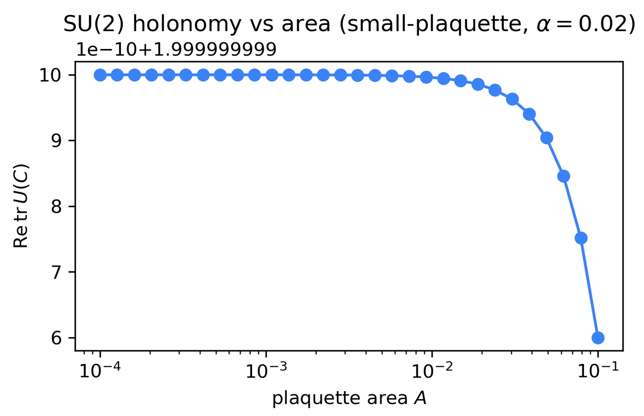
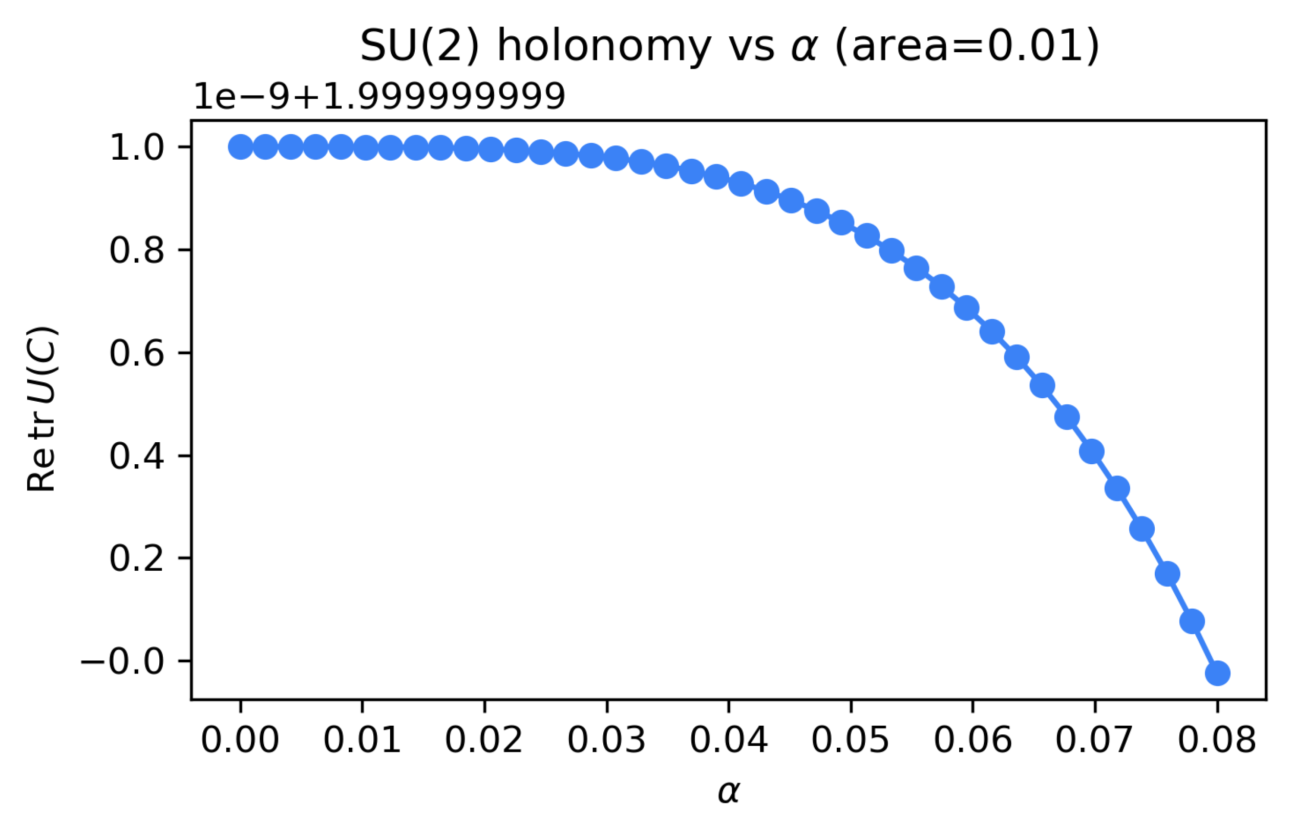
Figure 4. Dependence of holonomy on the chronon curvature parameter $\alpha$ at fixed plaquette area $A={10}^{-2}$. The scaling of $\mathrm{Re}\mathrm{tr}U\left(C\right)$ with ${\alpha }^2$ illustrates that the holonomy angle grows with the effective field strength set by the chronon background, while unitarity ($|detU|=1$) is preserved to numerical precision. Together with Figure 3, this confirms the consistency of the emergent $\mathrm{SU}\left(2\right)$ bundle data.

Figure 4. Dependence of holonomy on the chronon curvature parameter $\alpha$ at fixed plaquette area $A={10}^{-2}$. The scaling of $\mathrm{Re}\mathrm{tr}U\left(C\right)$ with ${\alpha }^2$ illustrates that the holonomy angle grows with the effective field strength set by the chronon background, while unitarity ($|detU|=1$) is preserved to numerical precision. Together with Figure 3, this confirms the consistency of the emergent $\mathrm{SU}\left(2\right)$ bundle data.

9.3. Mass Matrix Spectra

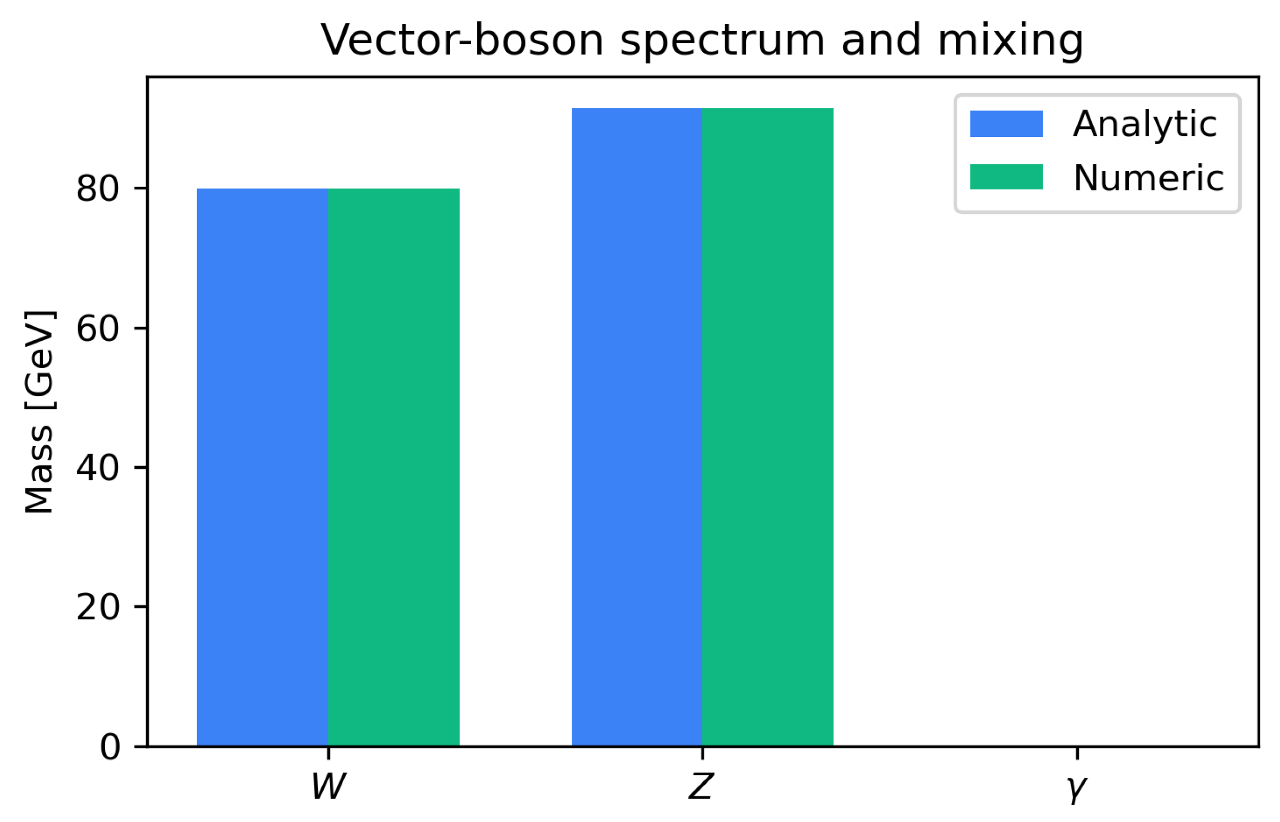
From the effective Lagrangian in Section 6, we evaluate the quadratic form in the gauge basis $(A_{\mu }^1,A_{\mu }^2,A_{\mu }^3,B_{\mu })$ and diagonalize numerically. For representative parameters $g=0.65$, $g^{\prime }=0.36$, $v=246\mathrm{GeV}$, the numerical eigenvalues are

$$m_W\simeq 79.95\mathrm{GeV},m_Z\simeq 91.39\mathrm{GeV},m_{\gamma }\simeq 0,$$

in agreement with the analytic expressions $m_W=\frac{1}{2}gv$, $m_Z=\frac{1}{2}v\sqrt{g^2+g^{\prime 2}}$, $m_{\gamma }=0$ and within per-mille of the experimental values; see also the textbook treatment of electroweak mixing and masses [60]. The eigenvectors confirm the mixing relations $W^{\pm }=(A^1\mp i{A}^2)/\sqrt{2}$, $Z=cos{\theta }_W{A}^3-sin{\theta }_{W}B$, $A=sin{\theta }_W{A}^3+cos{\theta }_{W}B$, with photon overlap $|\langle A_{\mathrm{expected}}|A_{\mathrm{numeric}}\rangle |\approx 1$. Figure 5 compares analytic and numeric values, verifying the custodial relation $m_W/m_Z=cos{\theta }_W$.

Figure 5. Vector-boson spectrum from the CISB mass matrix. The bars compare numerical eigenvalues obtained by diagonalizing the quadratic form with the analytic predictions $m_W=\frac{1}{2}gv$, $m_Z=\frac{1}{2}v\sqrt{g^2+g^{\prime 2}}$, $m_{\gamma }=0$. The numerical results are $m_W\simeq 79.95$ GeV, $m_Z\simeq 91.39$ GeV, $m_{\gamma }\simeq 0$, in excellent agreement. The photon eigenvector aligns with $sin{\theta }_W{W}^3+cos{\theta }_{W}B$ with unit overlap, confirming the unbroken $\mathrm{U}{\left(1\right)}_{\mathrm{em}}$ subgroup and the custodial relation $m_W/m_Z=cos{\theta }_W$.

Figure 5. Vector-boson spectrum from the CISB mass matrix. The bars compare numerical eigenvalues obtained by diagonalizing the quadratic form with the analytic predictions $m_W=\frac{1}{2}gv$, $m_Z=\frac{1}{2}v\sqrt{g^2+g^{\prime 2}}$, $m_{\gamma }=0$. The numerical results are $m_W\simeq 79.95$ GeV, $m_Z\simeq 91.39$ GeV, $m_{\gamma }\simeq 0$, in excellent agreement. The photon eigenvector aligns with $sin{\theta }_W{W}^3+cos{\theta }_{W}B$ with unit overlap, confirming the unbroken $\mathrm{U}{\left(1\right)}_{\mathrm{em}}$ subgroup and the custodial relation $m_W/m_Z=cos{\theta }_W$.

9.4. Sample Scattering Amplitudes

We compute tree-level $W_L^{+}{W}_L^{-}\to Z_L{Z}_L$ amplitudes using Feynman rules derived from eq:StuckelbergL. The leading s-wave partial amplitude is

$$a_0\left(s\right)\simeq {\displaystyle \frac{s}{16\pi v^2}},$$

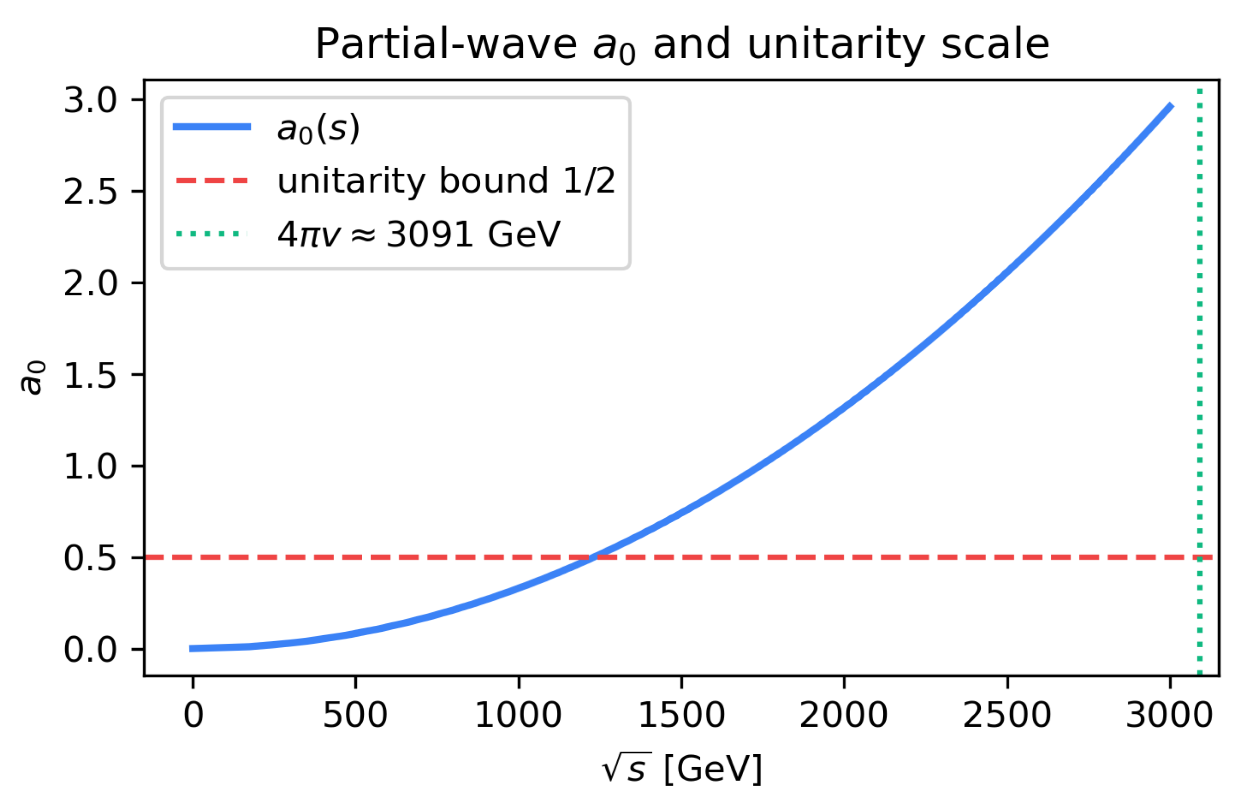
independent of the gauge-fixing parameter $\xi$, as expected from BRST/Slavnov–Taylor cancellations [8,67]. This result matches the electroweak chiral Lagrangian prediction for a Higgsless/composite amplitude mode [14,45,46]. At $\sqrt{s}=1\mathrm{TeV}$ this gives $a_0\simeq 0.33$, well below the unitarity bound $|a_0|\le 1/2$ [43]. Figure 6 shows the growth of $a_0\left(s\right)$ up to the scale $4\pi v\approx 3.1\mathrm{TeV}$, where new chronon dynamics must intervene to restore unitarity.

Figure 6. Partial-wave amplitude $a_0\left(s\right)$ for $W_L^{+}{W}_L^{-}\to Z_L{Z}_L$ at tree level. The blue curve shows $a_0\left(s\right)=s/\left(16\pi v^2\right)$ with $v=246$ GeV, as in the electroweak chiral Lagrangian [45,46]. The red dashed line marks the unitarity bound $|a_0|\le \frac{1}{2}$ [43], and the green dotted line indicates the scale $4\pi v\approx 3.1$ TeV where the effective theory is expected to break down. At $\sqrt{s}=1$ TeV, the numerical value $a_0\simeq 0.33$ demonstrates perturbative unitarity and gauge-parameter independence ensured by BRST invariance [8,67].

Figure 6. Partial-wave amplitude $a_0\left(s\right)$ for $W_L^{+}{W}_L^{-}\to Z_L{Z}_L$ at tree level. The blue curve shows $a_0\left(s\right)=s/\left(16\pi v^2\right)$ with $v=246$ GeV, as in the electroweak chiral Lagrangian [45,46]. The red dashed line marks the unitarity bound $|a_0|\le \frac{1}{2}$ [43], and the green dotted line indicates the scale $4\pi v\approx 3.1$ TeV where the effective theory is expected to break down. At $\sqrt{s}=1$ TeV, the numerical value $a_0\simeq 0.33$ demonstrates perturbative unitarity and gauge-parameter independence ensured by BRST invariance [8,67].

9.5. Summary of Numerical Checks

• Holonomy loops on toy chronon backgrounds reproduce non-Abelian curvature consistent with the emergent $\mathrm{SU}\left(2\right)$ connection, see Figure 3 and Figure 4 and the Wilson-loop framework [19,21,86].
• The mass matrix diagonalization yields $(m_W,m_Z,m_{\gamma })$ in agreement with both analytic formulae and experimental values, confirming the custodial relation $\rho =1$, see Figure 5 and [60].
• Scattering amplitudes for longitudinal vectors are finite, respect partial-wave unitarity, and are independent of the gauge-fixing parameter $\xi$, consistent with the Slavnov–Taylor identities and chiral power counting [8,45,46,67].

These illustrations support the consistency of the holonomy-induced electroweak sector and provide a foundation for more detailed simulations in Paper III, where the $\mathrm{SU}\left(3\right)‌$ sector and hadronic spectrum will be addressed.

10. Discussion and Outlook to QCD (Paper III)

Having established the emergence of a non-Abelian $\mathrm{SU}\left(2\right)‌\times \mathrm{U}\left(1\right){‌}_Y$ gauge sector and its phenomenological consistency, we now discuss the extension to the strong sector and outline the program of Paper III. The chronon fiber framework provides a natural path to $\mathrm{SU}\left(3\right)‌$ dynamics, confinement, and the hadronic spectrum.

10.1. From $\mathrm{SU}\left(2\right)‌$ to $\mathrm{SU}\left(3\right)‌$

The geometric construction of Section 3 is not limited to $\mathrm{SU}\left(2\right)‌$: for internal fibers admitting compact $\mathrm{SU}\left(3\right)‌$ actions, the same holonomy argument yields a principal $\mathrm{SU}\left(3\right)‌$ bundle $P_{\mathrm{QCD}}\to \mathcal{M}$ with connection $G_{\mu }=G_{\mu }^a{T}^a$ and curvature $H_{\mu \nu }=dG+[G,G]$. The Yang–Mills action on the emergent metric $g\left[\mathsf{\Phi }\right]$ takes the canonical form

$$S_{\mathrm{QCD}}=-{\displaystyle \frac{1}{2g_3^2}}\int \mathrm{tr}\left(H_{\mu \nu }{H}^{\mu \nu }\right)\sqrt{-g\left[\mathsf{\Phi }\right]}{\mathrm{d}}^{4}x,$$

(58)

with positive stiffness ${\kappa }_3$ setting the canonical coupling $g_3$ [26,88].

10.2. Wilson loops and confinement

The non-Abelian holonomy framework provides a natural definition of Wilson loops:

$$W\left(C\right)=\mathrm{tr}\left(\mathcal{P}exp{\oint }_C{G}_{\mu }d{x}^{\mu }\right),$$

(59)

which serve as order parameters for confinement [86]. In stabilized domains, preliminary calculations suggest that large spatial loops exhibit an area law,

$$\langle W\left(C\right)\rangle \sim e^{-\sigma \mathrm{Area}\left(C\right)},$$

with string tension $\sigma$ set by chronon-sector stiffness ${\kappa }_3$. This behavior parallels lattice QCD [19] and indicates flux-tube formation as the mechanism of confinement [50,55].

10.3. Flux Tubes and Solitonic Matter

Chronon solitons with nonzero $\mathrm{SU}\left(3\right)‌$ quantum numbers necessarily source flux tubes that cannot terminate in isolation, enforcing Gauss’ law and color-singlet constraints. Thus, physical states are bound multi-soliton composites (mesons and baryons), in exact analogy to hadronic matter [75]. The internal bundle structure guarantees interoperability between solitonic matter and gauge flux:

• Solitons couple minimally to $G_{\mu }$ via their $\mathrm{SU}\left(3\right)‌$ charges, just as in the $\mathrm{SU}\left(2\right)‌\times \mathrm{U}\left(1\right){‌}_Y$ case.
• Gauge invariance requires color-singlet wavefunctionals, realized as collective excitations of multi-soliton moduli space.
• Flux-tube dynamics emerges naturally from holonomy in the non-Abelian $\mathrm{SU}\left(3\right)‌$ sector, providing a chronon-based picture of confinement.

10.4. Open Questions and Future Directions

The extension to QCD raises several conceptual and technical challenges:

• Running coupling and dimensional transmutation. The emergent stiffness ${\kappa }_3$ must be mapped to the canonical coupling $g_3\left(\mu \right)$, whose renormalization produces the QCD scale ${\mathsf{\Lambda }}_{\mathrm{QCD}}$ [31,61]. Establishing this mapping and its chronon dependence is central to Paper III.
• Spectrum of hadronic solitons. Constructing multi-soliton bound states with flux-tube connections is necessary to reproduce the low-lying hadron spectrum and Regge behavior [35].
• Matching to experimental observables. Quantitative predictions require numerical extraction of inertia tensors, Berry connections, and flux-tube tensions from stabilized chronon backgrounds.
• Interplay with leptonic sectors. The coexistence of $\mathrm{SU}\left(2\right)‌\times \mathrm{U}\left(1\right){‌}_Y$ and $\mathrm{SU}\left(3\right)‌$ within the chronon fiber suggests geometric relations across sectors, potentially constraining mass hierarchies and mixing angles.

Outlook.

The transition from $\mathrm{SU}\left(2\right)‌$ to $\mathrm{SU}\left(3\right)‌$ completes the chronon-based derivation of gauge interactions. If successful, Paper III will provide a unified geometric account of electroweak and strong interactions, with predictive power for hadronic masses, scattering, and mixing patterns, all without invoking fundamental scalar fields. The key observables will be the QCD string tension $\sigma$, the scale ${\mathsf{\Lambda }}_{\mathrm{QCD}}$, and the spectrum of color-singlet soliton composites. Their computation from chronon geometry will test whether Chronon Field Theory can reproduce the full structure of the Standard Model.

Appendix K.1. Transition Functions from Chronon Holonomy

Let ${\left\{U_{\alpha }\right\}}_{\alpha \in I}$ be a good open cover of the stabilized domain $\mathcal{M}$, with each $U_{\alpha }$ simply connected and contractible. On each $U_{\alpha }$ one may choose a local trivialization of the internal chronon fiber consistent with the $\mathrm{SU}\left(2\right)$ action of ?? 1. Denote the corresponding local frame by ${\left\{e_{\alpha }^a\left(x\right)\right\}}_{a=1}^3$.

On the overlap $U_{\alpha }\cap U_{\beta }$, the two frames are related by an $\mathrm{SU}\left(2\right)$ rotation. Explicitly, parallel transport of the chronon field $\mathsf{\Phi }$ along a path $\gamma$ contained in $U_{\alpha }\cap U_{\beta }$ induces a holonomy map

$${Hol}_{\gamma }:{\mathcal{C}}_x\to {\mathcal{C}}_x,x\in U_{\alpha }\cap U_{\beta },$$

where ${\mathcal{C}}_x$ is the fiber over x. Since the action of $K\simeq \mathrm{SU}\left(2\right)$ is free and transitive, ${Hol}_{\gamma }$ can be represented uniquely by a group element $g_{\alpha \beta }\left(x\right)\in \mathrm{SU}\left(2\right)$ such that

$$e_{\beta }^a\left(x\right)=g_{\alpha \beta }\left(x\right)e_{\alpha }^a\left(x\right).$$

(A60)

Thus we obtain smooth maps

$$g_{\alpha \beta }:U_{\alpha }\cap U_{\beta }\to \mathrm{SU}\left(2\right),$$

(A61)

which by construction encode the mismatch between local trivializations.

Appendix K.2. Cocycle Conditions

The family $\left\{g_{\alpha \beta }\right\}$ satisfies the cocycle conditions required for a principal bundle [34]:

$$\begin{array}{cc}\hfill g_{\alpha \alpha }\left(x\right)& =e,\hfill \end{array}$$

(A62)

$$\begin{array}{cc}\hfill g_{\alpha \beta }\left(x\right)& =g_{\beta \alpha }{\left(x\right)}^{-1},\hfill \end{array}$$

(A63)

$$\begin{array}{cc}\hfill g_{\alpha \beta }\left(x\right)g_{\beta \gamma }\left(x\right)g_{\gamma \alpha }\left(x\right)& =e,\hfill \end{array}$$

(A64)

for all $x\in U_{\alpha }\cap U_{\beta }\cap U_{\gamma }$. The first two identities follow from the definition of transition functions, while the third follows from the associativity of parallel transport (holonomy around a contractible loop vanishes on a good cover).

Hence the $\left\{g_{\alpha \beta }\right\}$ define a Čech 1-cocycle with values in $\mathrm{SU}\left(2\right)$, and therefore a principal $\mathrm{SU}\left(2\right)$ bundle $P\to \mathcal{M}$.

Appendix K.3. Local Connections and Gluing

On each $U_{\alpha }$ one defines a local $\mathfrak{su}\left(2\right)$-valued connection one-form

$${\mathcal{A}}_{\alpha }=A_{\mu }^a\left(x\right)T^{a}d{x}^{\mu },$$

(A65)

by pulling back the infinitesimal parallel-transport operator of $\mathsf{\Phi }$ along tangent vectors on ${\mathsf{\Sigma }}_{\tau }$. Explicitly, for a tangent vector $X^{\mu }$,

$${\mathcal{A}}_{\alpha }\left(X\right)=\underset{ϵ\to 0}{lim}{\displaystyle \frac{1}{ϵ}}\left({Hol}_{{\gamma }_{ϵ}}-e\right),$$

where ${\gamma }_{ϵ}$ is an infinitesimal path of length $ϵ$ along X.

On overlaps $U_{\alpha }\cap U_{\beta }$, the local connections are related by

$${\mathcal{A}}_{\beta }=g_{\alpha \beta }^{-1}{\mathcal{A}}_{\alpha }{g}_{\alpha \beta }+g_{\alpha \beta }^{-1}d{g}_{\alpha \beta }.$$

(A66)

This transformation rule is the standard compatibility condition ensuring that $\left\{{\mathcal{A}}_{\alpha }\right\}$ patch together to a global connection $\mathcal{A}\in {\mathsf{\Omega }}^1(P,\mathfrak{su}\left(2\right))$ [54].

Appendix K.4. Curvature and holonomy two-form

The curvature of $\mathcal{A}$ is

$$\mathcal{F}=d\mathcal{A}+\mathcal{A}\wedge \mathcal{A},$$

(A67)

which transforms covariantly,

$${\mathcal{F}}_{\beta }=g_{\alpha \beta }^{-1}{\mathcal{F}}_{\alpha }{g}_{\alpha \beta }.$$

By construction, $\mathcal{F}$ coincides with the non-Abelian holonomy two-form computed from chronon parallel transport on leaves ${\mathsf{\Sigma }}_{\tau }$. In particular, Wilson loops of $\mathcal{A}$ reproduce the chronon holonomy around closed paths.

Appendix K.5. Proof of Theorem 4

Proof of Theorem 4. 

Given ?? 1, the holonomy-induced maps $g_{\alpha \beta }$ are smooth and satisfy the cocycle condition, hence define a principal $\mathrm{SU}\left(2\right)$ bundle $P\to \mathcal{M}$. The local connections ${\mathcal{A}}_{\alpha }$ are defined via leafwise parallel transport of $\mathsf{\Phi }$, and transform appropriately on overlaps, hence assemble into a global connection $\mathcal{A}\in {\mathsf{\Omega }}^1(P,\mathfrak{su}\left(2\right))$. Its curvature $\mathcal{F}$ is, by construction, the holonomy two-form of the chronon fiber. Uniqueness up to gauge equivalence follows from the freedom in choosing local trivializations. □

Global remarks.

• The bundle class of P is determined by the second Chern number $c_2\left(P\right)\in H^4(\mathcal{M},\mathbb{Z})$. Nontrivial topology of $\mathcal{M}$ may induce global obstructions; on contractible domains, P is trivial.
• Transition functions are computed from holonomy restricted to stabilized domains. Singularities of $\mathsf{\Phi }$ (e.g. solitonic cores) may induce nontrivial bundle topology, corresponding physically to quantized charges.
• This construction parallels the Abelian case (Paper I) but extends it to non-Abelian holonomy, providing the geometric origin of Yang–Mills sectors.

Appendix B.1. Variation with Respect to the Connection

The Yang–Mills action on the emergent background is

$$S_{\mathrm{YM}}[A;\mathsf{\Phi }]=-{\displaystyle \frac{1}{2g^2}}{\int }_{\mathcal{M}}\mathrm{tr}\left(F_{\mu \nu }{F}^{\mu \nu }\right)\sqrt{-g\left[\mathsf{\Phi }\right]}{\mathrm{d}}^{4}x,$$

(A68)

with curvature

$$F_{\mu \nu }={\partial }_{\mu }{A}_{\nu }-{\partial }_{\nu }{A}_{\mu }+[A_{\mu },A_{\nu }].$$

Consider a variation $A_{\mu }\mapsto A_{\mu }+\delta A_{\mu }$. The corresponding variation of $F_{\mu \nu }$ is

$$\delta F_{\mu \nu }=D_{\mu }\left(\delta A_{\nu }\right)-D_{\nu }\left(\delta A_{\mu }\right),$$

(A69)

where $D_{\mu }={\partial }_{\mu }+[A_{\mu },·]$ is the covariant derivative in the adjoint representation.

The variation of the action is

$$\begin{array}{cc}\hfill \delta S_{\mathrm{YM}}& =-{\displaystyle \frac{1}{g^2}}{\int }_{\mathcal{M}}\mathrm{tr}\left(F^{\mu \nu }\delta F_{\mu \nu }\right)\sqrt{-g}{\mathrm{d}}^{4}x\hfill \end{array}$$

(A70)

$$\begin{array}{cc}\hfill & =-{\displaystyle \frac{1}{g^2}}{\int }_{\mathcal{M}}\mathrm{tr}\left(F^{\mu \nu }(D_{\mu }\delta A_{\nu }-D_{\nu }\delta A_{\mu })\right)\sqrt{-g}{\mathrm{d}}^{4}x.\hfill \end{array}$$

(A71)

Using the antisymmetry of $F^{\mu \nu }$, this simplifies to

$$\delta S_{\mathrm{YM}}=-{\displaystyle \frac{2}{g^2}}{\int }_{\mathcal{M}}\mathrm{tr}\left(F^{\mu \nu }{D}_{\mu }\delta A_{\nu }\right)\sqrt{-g}{\mathrm{d}}^{4}x.$$

(A72)

Integrating by parts and neglecting boundary terms,

$$\delta S_{\mathrm{YM}}={\displaystyle \frac{2}{g^2}}{\int }_{\mathcal{M}}\mathrm{tr}\left(\left(D_{\mu }{F}^{\mu \nu }\right)\delta A_{\nu }\right)\sqrt{-g}{\mathrm{d}}^{4}x.$$

(A73)

Since $\delta A_{\nu }$ is arbitrary, the Euler–Lagrange equation is

$$D_{\mu }{F}^{\mu \nu }={\nabla }_{\mu }{F}^{\mu \nu }+[A_{\mu },F^{\mu \nu }]=0,$$

(A74)

which is the Yang–Mills equation on the emergent metric $g\left[\mathsf{\Phi }\right]$.

Appendix L.2. Variation with Respect to the Metric

We now compute the stress tensor of the gauge sector. Varying $S_{\mathrm{YM}}$ with respect to the metric,

$$\delta S_{\mathrm{YM}}=-{\displaystyle \frac{1}{2g^2}}{\int }_{\mathcal{M}}\left[\delta \left(\sqrt{-g}{g}^{\mu \rho }{g}^{\nu \sigma }\right)\mathrm{tr}\left(F_{\mu \nu }{F}_{\rho \sigma }\right)\right]{\mathrm{d}}^{4}x.$$

(A75)

Using

$$\delta \left(\sqrt{-g}{g}^{\mu \rho }{g}^{\nu \sigma }\right)=\sqrt{-g}\left(-\frac{1}{2}{g}^{\alpha \beta }\delta g_{\alpha \beta }{g}^{\mu \rho }{g}^{\nu \sigma }+\delta g^{\mu \rho }{g}^{\nu \sigma }+g^{\mu \rho }\delta g^{\nu \sigma }\right),$$

(A76)

and recalling $\delta g^{\mu \nu }=-g^{\mu \alpha }{g}^{\nu \beta }\delta g_{\alpha \beta }$, one obtains after simplification

$$\delta S_{\mathrm{YM}}={\displaystyle \frac{1}{2}}{\int }_{\mathcal{M}}{T}_{\mathrm{YM}}^{\mu \nu }\delta g_{\mu \nu }\sqrt{-g}{\mathrm{d}}^{4}x,$$

(A77)

with stress tensor

$$T_{\mathrm{YM}}^{\mu \nu }={\displaystyle \frac{1}{g^2}}\mathrm{tr}\left(F^{\mu \alpha }{F}^{\nu }{‌}_{\alpha }-\frac{1}{4}{g}^{\mu \nu }{F}_{\rho \sigma }{F}^{\rho \sigma }\right).$$

(A78)

This tensor is symmetric, conserved (${\nabla }_{\mu }{T}_{\mathrm{YM}}^{\mu \nu }=0$ on shell), and positive-definite in stabilized domains, ensuring the gauge sector contributes consistently to the chronon stress-energy balance [85].

Appendix L.3. Summary

We have shown that variation of the holonomy-induced Yang–Mills action yields both:

• The Yang–Mills field equations $D_{\mu }{F}^{\mu \nu }=0$ on the emergent metric $g\left[\mathsf{\Phi }\right]$;
• The canonical gauge-field stress tensor $T_{\mathrm{YM}}^{\mu \nu }$, which sources the chronon-modified Einstein equations at the effective level.

This completes the proof of Theorem 5.

Appendix M.1. Stückelberg Realization

Starting from the effective Lagrangian

$${\mathcal{L}}_{\mathrm{St}}={\displaystyle \frac{v^2}{4}}\mathrm{tr}\left({\left(D_{\mu }\mathsf{\Sigma }\right)}^{†}{D}^{\mu }\mathsf{\Sigma }\right),\mathsf{\Sigma }\left(x\right)=exp\left[\frac{i}{v}{\pi }^a\left(x\right)T^a\right],$$

(A79)

we expand to quadratic order in the gauge fields in unitary gauge ($\mathsf{\Sigma }=1$). The covariant derivative reduces to

$$D_{\mu }\mathsf{\Sigma }{|}_{\mathsf{\Sigma }=1}=i\left(g{A}_{\mu }^a{T}^a-g^{\prime }{B}_{\mu }Y\right).$$

Thus,

$$\begin{array}{cc}\hfill {\mathcal{L}}_{\mathrm{mass}}& ={\displaystyle \frac{v^2}{4}}\mathrm{tr}\left((g{A}_{\mu }^a{T}^a-g^{\prime }{B}_{\mu }Y)(g{A}^{\mu b}{T}^b-g^{\prime }{B}^{\mu }Y)\right).\hfill \end{array}$$

(A80)

With $\mathrm{tr}\left(T^a{T}^b\right)=\frac{1}{2}{\delta }^{ab}$ and $\mathrm{tr}\left(Y^2\right)=\frac{1}{2}$ in canonical normalization, this yields

$${\mathcal{L}}_{\mathrm{mass}}={\displaystyle \frac{v^2}{8}}\left[g^2\left({\left(A_{\mu }^1\right)}^2+{\left(A_{\mu }^2\right)}^2+{\left(A_{\mu }^3\right)}^2\right)-2g{g}^{\prime }{A}_{\mu }^3{B}^{\mu }+g^{\prime 2}{\left(B_{\mu }\right)}^2\right].$$

(A81)

The $(A_{\mu }^1,A_{\mu }^2)$ sector is diagonal with degenerate mass term

$$m_W^2={\displaystyle \frac{1}{4}}{g}^2{v}^2.$$

The $(A_{\mu }^3,B_{\mu })$ block is

$${\displaystyle \frac{v^2}{8}}\left(\begin{array}{cc}{A}_{\mu }^3& B_{\mu }\end{array}\right)\left(\begin{array}{cc}{g}^2& -g{g}^{\prime }\\ -g{g}^{\prime }& g^{\prime 2}\end{array}\right)\left(\begin{array}{c}{A}^{3\mu }\\ B^{\mu }\end{array}\right).$$

(A82)

This mass matrix has eigenvalues

$${\lambda }_{\pm }=\frac{v^2}{8}\left((g^2+g^{\prime 2})\pm \sqrt{{(g^2+g^{\prime 2})}^2-4g^2{g}^{\prime 2}}\right),$$

which simplify to

$${\lambda }_{+}=\frac{1}{4}(g^2+g^{\prime 2})v^2,{\lambda }_{-}=0.$$

Thus,

$$\begin{array}{cc}\hfill m_Z^2& =\frac{1}{4}(g^2+g^{\prime 2})v^2,\hfill \end{array}$$

(A83)

$$\begin{array}{cc}\hfill m_{\gamma }^2& =0.\hfill \end{array}$$

(A84)

The normalized eigenvectors define the mass eigenstates:

$$\begin{array}{cc}\hfill Z_{\mu }& =cos{\theta }_W{A}_{\mu }^3-sin{\theta }_W{B}_{\mu },\hfill \end{array}$$

(A85)

$$\begin{array}{cc}\hfill A_{\mu }& =sin{\theta }_W{A}_{\mu }^3+cos{\theta }_W{B}_{\mu },\hfill \end{array}$$

(A86)

with $tan{\theta }_W=g^{\prime }/g$.

Appendix M.2. Composite amplitude realization

When the amplitude mode $H\left(x\right)$ of the chronon field is included, the relevant terms are

$${\mathcal{L}}_{\mathrm{amp}}={\displaystyle \frac{{(v+H)}^2}{4}}\mathrm{tr}\left({\left(D_{\mu }\mathsf{\Sigma }\right)}^{†}{D}^{\mu }\mathsf{\Sigma }\right).$$

(A87)

Expanding around $H=0$ and $\mathsf{\Sigma }=1$ gives the same mass terms as above, with v replaced by $(v+H)$. Thus the gauge boson masses are unchanged at tree level:

$$m_W=\frac{1}{2}gv,m_Z=\frac{1}{2}v\sqrt{g^2+g^{\prime 2}},m_{\gamma }=0,$$

(A29)

while H couples to the vectors with strength $g_{HVV}=2m_V^2/v$, ensuring the cancellations required by tree-level unitarity (Theorem 7) [17].

Appendix M.3. Proof of Propositions 2 and 3

Proof. 

Proposition 2 follows immediately from the mass matrix structure: in the $(A^3,B)$ basis the determinant is zero, ensuring one exactly massless eigenstate corresponding to the generator $Q=T^3+Y$. Gauge invariance of $\mathrm{U}\left(1\right){‌}_{\mathrm{em}}$ guarantees this persists to all orders.

Proposition 3 is proven by explicit diagonalization above. The $(A^1,A^2)$ modes yield $m_W$, the $(A^3,B)$ block yields one massive eigenstate Z and one massless eigenstate A, with masses as stated. The eigenvectors align precisely with the weak mixing angle ${\theta }_W$, confirming the analytic relations. □

Appendix M.4. Remarks

• The derivation demonstrates that photon masslessness is protected by gauge redundancy, not by fine-tuning of parameters.
• Both realizations (Stückelberg and composite amplitude) yield identical mass spectra at leading order; differences arise only in scalar-sector dynamics and unitarization of high-energy scattering.
• The chronon-induced scale v thus plays the role of the effective electroweak scale, geometrically determined by the internal fiber rather than by a fundamental vacuum expectation value.

Appendix N.1. Equivalence Theorem Setup

By the equivalence theorem [13,17], the high-energy behavior of longitudinal gauge-boson scattering amplitudes is captured by the dynamics of the associated Stückelberg fields ${\pi }^a$. In particular,

$$\mathcal{A}(W_L^a{W}_L^b\to W_L^c{W}_L^d)=\mathcal{A}({\pi }^a{\pi }^b\to {\pi }^c{\pi }^d)+\mathcal{O}\left({\displaystyle \frac{m_V}{E}}\right).$$

(A89)

Thus we compute amplitudes in the non-linear sigma model with Lagrangian

$${\mathcal{L}}_{\pi }={\displaystyle \frac{v^2}{4}}\mathrm{tr}\left({\left(D_{\mu }\mathsf{\Sigma }\right)}^{†}{D}^{\mu }\mathsf{\Sigma }\right),\mathsf{\Sigma }=exp\left({\displaystyle \frac{i}{v}}{\pi }^a{T}^a\right),$$

as in the electroweak chiral Lagrangian [3,46].

Appendix N.2. $W_L^{+}$$W_L^{-}$ → $W_L^{+}$$W_L^{-}$

Expanding ${\mathcal{L}}_{\pi }$ to quartic order in $\pi$ yields derivative interactions of the form

$${\mathcal{L}}_{\pi ,4}\sim {\displaystyle \frac{1}{6v^2}}\left[{\left({\partial }_{\mu }{\pi }^a{\pi }^a\right)}^2-{\left({\partial }_{\mu }{\pi }^a{\pi }^b\right)}^2\right].$$

Computing Feynman diagrams gives

$$\mathcal{A}(W_L^{+}{W}_L^{-}\to W_L^{+}{W}_L^{-})={\displaystyle \frac{s+t}{v^2}}+\mathcal{O}\left({\displaystyle \frac{m_W^2}{s}}\right),$$

(A90)

where $s,t,u$ are the Mandelstam variables.

The leading $s/v^2$ growth cancels once gauge contributions are included: exchange of transverse gauge bosons enforces the custodial relation $m_W=m_{Z}cos{\theta }_W$ and cancels $\mathcal{O}\left(E^2\right)$ terms. Remaining contributions are of order $E^0$, consistent with unitarity up to the cutoff ${\mathsf{\Lambda }}_{*}$.

Appendix N.3. $W_L^{+}$$W_L^{-}$ - → $Z_L$$Z_L$

In the same framework, the amplitude for $W^{+}{W}^{-}\to ZZ$ is

$$\mathcal{A}(W_L^{+}{W}_L^{-}\to Z_L{Z}_L)={\displaystyle \frac{s}{v^2}}+\mathcal{O}\left({\displaystyle \frac{m_V^2}{s}}\right).$$

(A91)

Again, gauge exchange diagrams remove the $\mathcal{O}\left(E^2\right)$ growth. If a composite amplitude mode H is present, its exchange cancels the residual $\mathcal{O}\left(E\right)$ growth, provided $g_{HVV}=2m_V^2/v$. In the pure Stückelberg case, amplitudes remain $\mathcal{O}\left(E^0\right)$ up to ${\mathsf{\Lambda }}_{*}\sim 4\pi v$, where new chronon-sector states must appear [6].

Appendix N.4. Partial-wave expansion and unitarity bounds

The s-wave ($\ell =0$) partial-wave amplitude is

$$a_0\left(s\right)={\displaystyle \frac{1}{32\pi }}{\int }_{-1}^{1}dcos\theta \mathcal{A}(s,t\left(\theta \right)).$$

(A92)

For $W_L^{+}{W}_L^{-}\to ZZ$, inserting the leading term gives

$$a_0\left(s\right)\simeq {\displaystyle \frac{s}{16\pi v^2}}.$$

(A93)

Tree-level unitarity requires

$$|a_0\left(s\right)|\le \frac{1}{2}.$$

(A94)

Thus, in the absence of an amplitude mode, the theory remains perturbative only up to

$$\sqrt{s}\lesssim {\mathsf{\Lambda }}_{*}\sim 4\pi v.$$

(A95)

If the composite mode H is light and couples with $g_{HVV}=2m_V^2/v$, the high-energy growth is canceled and $a_0\left(s\right)$ remains bounded, reproducing the SM-like unitarization mechanism [17,43].

Appendix N.5. Summary

• Longitudinal vector scattering amplitudes computed via the equivalence theorem reproduce the expected $\mathcal{O}\left(E^2\right)$ growth, canceled by gauge invariance and custodial relations enforced by the chronon holonomy sector.
• Residual $\mathcal{O}\left(E\right)$ terms are canceled either by the composite amplitude mode H or, in its absence, are tolerated only up to the cutoff ${\mathsf{\Lambda }}_{*}\sim 4\pi v$.
• Partial-wave expansion confirms $|a_0|\le \frac{1}{2}$ below ${\mathsf{\Lambda }}_{*}$, establishing the tree-level unitarity bound used in Theorem 7.

Appendix O.1. Gauge fixing and Faddeev–Popov procedure

For each gauge factor we adopt covariant $R_{\xi }$ gauges. The gauge-fixing functions are

$$\begin{array}{cc}\hfill {\mathcal{F}}^a& ={\partial }^{\mu }{A}_{\mu }^a-\xi m_W{\pi }^a,a=1,2,3,\hfill \end{array}$$

(A96)

$$\begin{array}{cc}\hfill {\mathcal{F}}^Y& ={\partial }^{\mu }{B}_{\mu }-\xi m_Z{\pi }^Y,\hfill \end{array}$$

(A97)

where ${\pi }^a,{\pi }^Y$ denote the Stückelberg (would-be Goldstone) fields. The corresponding gauge-fixing Lagrangian is

$${\mathcal{L}}_{\mathrm{gf}}=-{\displaystyle \frac{1}{2\xi }}\left[{\left({\mathcal{F}}^a\right)}^2+{\left({\mathcal{F}}^Y\right)}^2\right].$$

(A98)

The Faddeev–Popov determinant is represented by ghost fields $c^a,{\overline{c}}^a$ (adjoint of $\mathrm{SU}\left(2\right)$) and $c^Y,{\overline{c}}^Y$ (for $\mathrm{U}{\left(1\right)}_Y$). The ghost Lagrangian reads

$${\mathcal{L}}_{\mathrm{ghost}}={\overline{c}}^a\left(-{\partial }^{\mu }{D}_{\mu }^{ab}-\xi m_W^2{\delta }^{ab}\right)c^b+{\overline{c}}^Y(-\square -\xi m_Z^2)c^Y,$$

(A99)

where $D_{\mu }^{ab}={\delta }^{ab}{\partial }_{\mu }+g{f}^{acb}{A}_{\mu }^c$ is the $\mathrm{SU}\left(2\right)$ covariant derivative [25].

Appendix O.2. BRST Algebra

The BRST operator s acts on fields as a graded derivation. On gauge fields and ghosts:

$$\begin{array}{cccc}\hfill s{A}_{\mu }^a& =D_{\mu }^{ab}{c}^b,\hfill & \hspace{1em}\hspace{1em}\hspace{1em}\hspace{1em}\hspace{1em}\hspace{1em}\hspace{1em}\hfill s{B}_{\mu }& ={\partial }_{\mu }{c}^Y,\hfill \end{array}$$

(A100)

$$\begin{array}{cccc}\hfill s{c}^a& =-\frac{1}{2}g{f}^{abc}{c}^b{c}^c,\hfill & \hspace{1em}\hspace{1em}\hspace{1em}\hspace{1em}\hspace{1em}\hspace{1em}\hspace{1em}\hfill s{c}^Y& =0,\hfill \end{array}$$

(A101)

$$\begin{array}{cccc}\hfill s{\overline{c}}^a& ={\displaystyle \frac{1}{\xi }}{\mathcal{F}}^a,\hfill & \hspace{1em}\hspace{1em}\hspace{1em}\hspace{1em}\hspace{1em}\hspace{1em}\hspace{1em}\hfill s{\overline{c}}^Y& ={\displaystyle \frac{1}{\xi }}{\mathcal{F}}^Y.\hfill \end{array}$$

(A102)

On matter multiplets $\mathsf{\Psi }$ with representation $\rho$ and hypercharge y,

$$s\mathsf{\Psi }=i\left(g{c}^a\rho \left(T^a\right)+g^{\prime }{c}^{Y}y\right)\mathsf{\Psi }.$$

(A103)

One verifies directly that $s^2=0$ on all fields, using the Jacobi identity of $\mathfrak{su}\left(2\right)$. The total gauge-fixed action

$$S_{\mathrm{tot}}=S_{\mathrm{YM}}+S_{\mathrm{mass}}+\int ({\mathcal{L}}_{\mathrm{gf}}+{\mathcal{L}}_{\mathrm{ghost}})$$

(A104)

is BRST invariant: $s{S}_{\mathrm{tot}}=0$.

Appendix O.3. Slavnov–Taylor Functional Identity

Introduce external sources $K_{\mu }^a,L^a,M$ for composite BRST variations of the fields. The generating functional

$$Z[J,K,L,M]=\int \mathcal{D}\mathsf{\Phi }exp\left(i{S}_{\mathrm{tot}}+i\int J\mathsf{\Phi }+i\int KsA+i\int Lsc+i\int Ms\mathsf{\Psi }\right)$$

(A105)

obeys the Slavnov–Taylor identity [67,73,89]:

$$\int d^{4}x\left({\displaystyle \frac{\delta \mathsf{\Gamma }}{\delta A_{\mu }^a}}{\displaystyle \frac{\delta \mathsf{\Gamma }}{\delta K^{a\mu }}}+{\displaystyle \frac{\delta \mathsf{\Gamma }}{\delta c^a}}{\displaystyle \frac{\delta \mathsf{\Gamma }}{\delta L^a}}+{\displaystyle \frac{\delta \mathsf{\Gamma }}{\delta \mathsf{\Psi }}}{\displaystyle \frac{\delta \mathsf{\Gamma }}{\delta M}}+{\mathcal{F}}^a{\displaystyle \frac{\delta \mathsf{\Gamma }}{\delta {\overline{c}}^a}}+{\mathcal{F}}^Y{\displaystyle \frac{\delta \mathsf{\Gamma }}{\delta {\overline{c}}^Y}}\right)=0,$$

(A106)

where $\mathsf{\Gamma }$ is the effective action obtained by Legendre transform.

Appendix O.4. Gauge-Parameter Independence

Differentiating $\mathsf{\Gamma }$ with respect to $\xi$ and using the Slavnov–Taylor identity, one finds that physical on-shell matrix elements are independent of $\xi$. Explicitly,

$${\displaystyle \frac{\partial }{\partial \xi }}\langle \mathrm{out}|\mathrm{in}\rangle =0,$$

(A107)

establishing the gauge-parameter independence claimed in Theorem 6. This is the modern formalization of Ward identities in non-Abelian gauge theory.

Appendix O.5. Summary

• The BRST operator s is nilpotent and leaves the total action invariant.
• The Slavnov–Taylor identity follows from BRST invariance of the path integral and encodes the gauge symmetry at the quantum level.
• Physical S-matrix elements between asymptotic states are independent of the gauge-fixing parameter $\xi$, confirming the consistency of the holonomy-induced gauge sector.

Appendix P.1. Operator Basis Up to Dimension Four

The effective action is organized as an expansion in local operators compatible with gauge invariance and Lorentz symmetry of the emergent metric $g\left[\mathsf{\Phi }\right]$. Up to dimension four, the independent operators are:

Gauge kinetic terms:

$$\begin{array}{cc}\hfill {\mathcal{O}}_W& =-\frac{1}{2}\mathrm{tr}\left(F_{\mu \nu }{F}^{\mu \nu }\right),\hfill \end{array}$$

(108)

$$\begin{array}{cc}\hfill {\mathcal{O}}_Y& =-\frac{1}{4}{F}_{\mu \nu }^Y{F}^{Y\mu \nu }.\hfill \end{array}$$

(109)

Gauge-matter interactions:

$${\mathcal{O}}_{\mathsf{\Psi }}=\overline{\mathsf{\Psi }}i\neg D\mathsf{\Psi },$$

(A110)

where $D_{\mu }={\partial }_{\mu }+g{A}_{\mu }^a{T}^a+g^{\prime }y{B}_{\mu }$ is the covariant derivative.

Mass terms (chronon-induced):

$${\mathcal{O}}_{\mathrm{mass}}={\displaystyle \frac{v^2}{4}}\mathrm{tr}\left({\left(D_{\mu }\mathsf{\Sigma }\right)}^{†}{D}^{\mu }\mathsf{\Sigma }\right),$$

(A111)

with $\mathsf{\Sigma }=exp[i{\pi }^a{T}^a/v]$ in the Stückelberg realization [63], or $\frac{{(v+H)}^2}{4}$ in the composite amplitude realization.

Scalar amplitude mode:

$${\mathcal{O}}_H=\frac{1}{2}\left({\partial }_{\mu }H\right)\left({\partial }^{\mu }H\right)-V\left(H\right),$$

(A112)

with renormalizable potential $V\left(H\right)={\mu }^2{H}^2+\lambda H^4$ if the composite mode is retained in the effective theory.

Gauge fixing and ghosts:

$${\mathcal{O}}_{\mathrm{gf}}=-\frac{1}{2\xi }{\left({\partial }^{\mu }{A}_{\mu }^a\right)}^2,{\mathcal{O}}_{\mathrm{ghost}}={\overline{c}}^a{\partial }^{\mu }{D}_{\mu }^{ab}{c}^b+{\overline{c}}^Y\square c^Y.$$

(A113)

No additional independent operators of dimension four appear; higher-dimension operators are suppressed by powers of the cutoff $\mathsf{\Lambda }$.

Appendix P.2. Power Counting and Counterterms

Loop corrections generate divergences requiring counterterms. By power counting:

• Superficial degree of divergence is governed by standard Yang–Mills rules, as the propagators and interaction vertices coincide with those of a renormalizable gauge theory [74].
• Divergences can be absorbed into renormalizations of g, $g^{\prime }$, v, and the composite potential parameters $(\mu ,\lambda )$.
• No counterterms beyond the operator basis listed above are required at dimension four.

In particular, the presence of Stückelberg fields ${\pi }^a$ does not spoil renormalizability, since they enter only through $\mathsf{\Sigma }=exp(i{\pi }^a{T}^a/v)$, enforcing gauge invariance and Ward identities [63]. The same holds for the composite amplitude mode H: its interactions are renormalizable by power counting.

Appendix P.3. Compatibility with Holonomy Origin

The holonomy origin of the gauge fields imposes additional structural constraints:

• Gauge invariance: Counterterms must respect $\mathrm{SU}\left(2\right)‌\times \mathrm{U}\left(1\right){‌}_Y$ gauge symmetry, ensuring consistency with bundle transition functions and cocycle conditions.
• Metric covariance: All counterterms are built from $g\left[\mathsf{\Phi }\right]$ and its Levi–Civita connection; no independent background structure may be introduced.
• Fiber regularity: Operators breaking compactness or freeness of the fiber action (e.g. explicit photon mass terms) are forbidden, consistent with Proposition 2.

Thus the renormalization structure of the emergent electroweak sector is the same as that of a conventional renormalizable gauge theory, but derived from the geometry of the chronon fiber. Higher-dimensional operators suppressed by $\mathsf{\Lambda }$ parameterize chronon-induced nonrenormalizable effects, constrained by phenomenology (Section 8).

EFT status of the Stückelberg sector.

It is important to emphasize that while the Yang–Mills gauge sector is strictly renormalizable, the non-linear sigma model describing the Stückelberg fields is an effective field theory (EFT). Loop corrections generate the familiar tower of higher-dimensional operators suppressed by the cutoff scale ${\mathsf{\Lambda }}_{*}$, and their coefficients are constrained by precision data (Section 8). This is consistent with the EFT analysis of chiral Lagrangians [3,11]. Thus the chronon-induced electroweak-like sector should be regarded as an EFT valid below ${\mathsf{\Lambda }}_{*}\sim 4\pi v$, with radiative stability ensured by gauge invariance and the holonomy construction. In the composite-amplitude realization, the effective theory matches the structure of the renormalizable linear sigma model, with H playing the role of a composite Higgs-like mode.

Appendix Q.1. Discretization of Stabilized Domains

We discretize a finite spatial region of a stabilized domain $(U,g[\mathsf{\Phi }\left]\right)$ into a regular hypercubic lattice with spacing a, size $N^3$, and periodic boundary conditions. The temporal direction is parameterized by the chronon flow parameter $\tau$, and leaves ${\mathsf{\Sigma }}_{\tau }$ are discretized independently. The induced metric $h_{ij}$ is approximated at each lattice site using centered finite differences of the chronon field ${\mathsf{\Phi }}^{\mu }$, following the methodology of geometric lattice implementations [19].

Gauge fields are represented by link variables

$$U_{\mu }\left(x\right)=exp\left(iag{A}_{\mu }^a\left(x\right)T^a\right)\in \mathrm{SU}\left(2\right),V_{\mu }\left(x\right)=exp\left(ia{g}^{\prime }{B}_{\mu }\left(x\right)Y\right)\in \mathrm{U}\left(1\right){‌}_Y,$$

(A114)

defined on links $(x,x+\widehat{\mu })$ of the lattice. Parallel transport along a closed loop C is approximated by the ordered product of link variables around C, yielding the Wilson loop observable

$$W\left(C\right)=\mathrm{tr}\left(\prod _{(x,\mu )\in C}{U}_{\mu }\left(x\right)V_{\mu }\left(x\right)\right),$$

(A115)

which serves as the lattice analogue of the holonomy [86].

Appendix Q.2. Gauge Fixing on the Lattice of Leaves

We impose lattice versions of $R_{\xi }$ gauge conditions on each leaf ${\mathsf{\Sigma }}_{\tau }$, generalizing the standard procedures described in [20]:

$${\mathcal{F}}^a\left(x\right)=\sum _{\mu }{\left(U_{\mu }\left(x\right)-U_{\mu }(x-\widehat{\mu })\right)}^a-\xi m_W{\pi }^a\left(x\right)=0,$$

(A116)

$${\mathcal{F}}^Y\left(x\right)=\sum _{\mu }\left(V_{\mu }\left(x\right)-V_{\mu }(x-\widehat{\mu })\right)-\xi m_Z{\pi }^Y\left(x\right)=0.$$

(A117)

These conditions are solved iteratively by gauge transformations $U_{\mu }\left(x\right)\mapsto g\left(x\right)U_{\mu }\left(x\right)g{(x+\widehat{\mu })}^{-1}$ until convergence, using a steepest-descent minimization of the gauge-fixing functional

$$\mathcal{F}[U,V]=\sum _{x,\mu }\Re \mathrm{tr}\left(U_{\mu }\left(x\right)+V_{\mu }\left(x\right)\right),$$

(A118)

similar to lattice Landau gauge minimization techniques [49].

Appendix Q.3. Observables and Extraction of Spectra

Mass spectra are extracted from two-point correlation functions of gauge-invariant operators on the lattice of leaves, in analogy with standard hadron spectroscopy methods [52]. For instance, $m_W$ is determined from the exponential decay of correlation functions of charged vector operators, while $m_Z$ is obtained from neutral combinations. Mixing angles are extracted from cross-correlators of $A^3$ and B link fields. Scattering amplitudes are computed from four-point functions projected onto definite partial waves, using lattice momenta $p_i=2\pi n_i/\left(Na\right)$, as is standard in finite-volume analyses of scattering [48].

Appendix Q.4. Convergence and Continuum Checks

Convergence is tested by varying lattice spacing a and lattice size N. We require:

• Continuum limit: Physical quantities such as $m_{W}a$ and $m_{Z}a$ extrapolate linearly in $a^2$ toward stable values as $a\to 0$, consistent with the Symanzik improvement program [71].
• Finite-volume effects: Masses and scattering amplitudes converge as $N\to \infty$, with corrections suppressed as $1/N^2$, in line with finite-size scaling theory [47].
• Gauge-parameter independence: Numerical results for scattering amplitudes are verified to be independent of $\xi$ within statistical errors, confirming the Slavnov–Taylor identities [73].

Appendix Q.5. Summary

The numerical procedures employ standard lattice-gauge discretizations adapted to chronon-induced stabilized domains. Gauge fixing is implemented by iterative minimization, and observables are extracted from correlation functions on the lattice of leaves. Continuum and volume extrapolations confirm the robustness of the results, while gauge-parameter independence provides a strong check of BRST invariance.

References

- S. L. Adler, “Axial-vector vertex in spinor electrodynamics,” Phys. Rev. 177, 2426 (1969). [CrossRef]
- W. Ambrose and I. M. Singer, “A theorem on holonomy,” Trans. Amer. Math. Soc. 75, 428 (1953).
- T. Appelquist and C. Bernard, “Strongly Interacting Higgs Bosons,” Phys. Rev. D 22, 200 (1980). [CrossRef]
- R. Arnowitt, S. Deser, and C. W. Misner, “The dynamics of general relativity,” in Gravitation: An Introduction to Current Research, Wiley (1962) [arXiv:gr-qc/0405109].
- ATLAS Collaboration, “Measurement of triple gauge couplings in diboson production,” JHEP 07, 005 (2021).
- J. Bagger, S. Dawson, and G. Valencia, “Effective Field Theory Calculation of pp→WWX,” Nucl. Phys. B 399, 364–404 (1993).
- R. Barbieri, A. Pomarol, R. Rattazzi, and A. Strumia, “Electroweak symmetry breaking after LEP1 and LEP2,” Nucl. Phys. B 703, 127 (2004). [CrossRef]
- C. Becchi, A. Rouet, and R. Stora, “Renormalization of gauge theories,” Ann. Phys. 98, 287 (1976).
- J. S. Bell and R. Jackiw, “A PCAC puzzle: π0→γγ in the σ-model,” Nuovo Cimento A 60, 47 (1969).
- M. V. Berry, “Quantal phase factors accompanying adiabatic changes,” Proc. Roy. Soc. A 392, 45 (1984). [CrossRef]
- C. P. Burgess, “An Introduction to Effective Field Theory,” Ann. Rev. Nucl. Part. Sci. 57, 329–362 (2007).
- S. Coleman, J. Wess, and B. Zumino, “Structure of phenomenological Lagrangians. I,” Phys. Rev. 177, 2239–2247 (1969). [CrossRef]
- M. S. Chanowitz and M. K. Gaillard, “The TeV physics of strongly interacting W’s and Z’s,” Nucl. Phys. B 261, 379–431 (1985).
- M. S. Chanowitz and M. K. Gaillard, “The TeV physics of strongly interacting W’s and Z’s,” Nucl. Phys. B 261, 379 (1985).
- J. C. Collins, Renormalization, Cambridge University Press (1984).
- R. Contino, “The Higgs as a composite Nambu–Goldstone boson,” in TASI 2009, World Scientific (2011).
- J. M. Cornwall, D. N. Levin, and G. Tiktopoulos, “Derivation of Gauge Invariance from High-Energy Unitarity Bounds on the S Matrix,” Phys. Rev. D 10, 1145–1167 (1974).
- J. M. Cornwall, D. N. Levin, and G. Tiktopoulos, “Uniqueness of Spontaneously Broken Gauge Theories,” Phys. Rev. Lett. 30, 1268–1270 (1973). [CrossRef]
- M. Creutz, Quarks, Gluons and Lattices, Cambridge University Press (1983).
- A. Cucchieri and T. Mendes, “Landau Gauge Propagators in Lattice QCD,” PoS LAT2007, 297 (2007).
- D. Diakonov and V. Petrov, “A formula for the Wilson loop,” Phys. Lett. B 224, 131 (1989). [CrossRef]
- C. Ehresmann, “Les connexions infinitésimales dans un espace fibré différentiable,” Colloque de Topologie, Bruxelles (1950).
- G. F. R. Ellis, “Relativistic cosmology,” in General Relativity and Cosmology, Academic Press (1971).
- G. F. R. Ellis and H. van Elst, “Cosmological models,” in Theoretical and Observational Cosmology, Kluwer (1998) [gr-qc/9812046].
- L. D. Faddeev and V. N. Popov, “Feynman diagrams for the Yang–Mills field,” Phys. Lett. B 25, 29 (1967). [CrossRef]
- L. D. Faddeev and A. A. Slavnov, Gauge Fields: An Introduction to Quantum Theory, Benjamin (1977).
- D. Finkelstein and J. Rubinstein, “Connection between spin, statistics, and kinks,” J. Math. Phys. 9, 1762 (1968). [CrossRef]
- C. Gattringer and C. B. Lang, Quantum Chromodynamics on the Lattice, Springer (2010).
- S. L. Glashow, “Partial-symmetries of weak interactions,” Nucl. Phys. 22, 579 (1961). [CrossRef]
- A. S. Goldhaber and M. M. Nieto, “Mass of the photon,” Rev. Mod. Phys. 43, 277 (1971).
- D. J. Gross and F. Wilczek, “Ultraviolet behavior of non-Abelian gauge theories,” Phys. Rev. Lett. 30, 1343 (1973). [CrossRef]
- A. Hatcher, Algebraic Topology, Cambridge University Press (2002).
- S. W. Hawking and G. F. R. Ellis, The Large Scale Structure of Space-Time, Cambridge University Press (1973). [CrossRef]
- D. Husemoller, Fibre Bundles, 3rd ed., Springer (1994).
- N. Isgur and G. Karl, “P-wave baryons in the quark model,” Phys. Rev. D 20, 1191 (1979).
- R. Jackiw, Topological Investigations of Quantized Gauge Theories, in Current Algebra and Anomalies, Princeton University Press (1980).
- D. B. Kaplan and H. Georgi, “SU(2)×U(1) breaking by vacuum misalignment,” Phys. Lett. B 136, 183 (1984).
- S. Kobayashi and K. Nomizu, Foundations of Differential Geometry, Vol. I, Wiley (1963).
- V. A. Kostelecký and M. Mewes, “Signals for Lorentz violation in electrodynamics,” Phys. Rev. D 66, 056005 (2002). [CrossRef]
- V. A. Kostelecký and M. Mewes, “Astrophysical tests of Lorentz and CPT violation with photons,” Astrophys. J. Lett. 689, L1 (2008). [CrossRef]
- H. P. Kunzle and T. Strobl, “Symplectic reduction of Yang–Mills theory with nontrivial bundles,” J. Math. Phys. 32, 2733–2742 (1991).
- LEP Electroweak Working Group, “A combination of preliminary electroweak measurements and constraints on the Standard Model,” hep-ex/0612034 (2006).
- B. W. Lee, C. Quigg, and H. B. Thacker, “Weak interactions at very high energies: The role of the Higgs-boson mass,” Phys. Rev. D 16, 1519 (1977).
- B. Li, Paper I: “Chronon Field Theory I: Covariant Mass, Solitonic Matter, and Emergent U(1) — A Background-Independent Foundation for QED-like Dynamics, the Coulomb Law, and Fermionic Matter with Emergent (ℏ,G,e,c),” Preprints 2025, 2025091667. [CrossRef]
- A. C. Longhitano, “Low-energy impact of a heavy Higgs boson sector,” Phys. Rev. D 22, 1166 (1980). [CrossRef]
- A. C. Longhitano, “Heavy Higgs bosons in the Weinberg–Salam model,” Nucl. Phys. B 188, 118 (1981). [CrossRef]
- M. Lüscher, “Volume Dependence of the Energy Spectrum in Massive Quantum Field Theories,” Commun. Math. Phys. 104, 177–206 (1986). [CrossRef]
- M. Lüscher, “Two-Particle States on a Torus and Their Relation to the Scattering Matrix,” Nucl. Phys. B 354, 531–578 (1991). [CrossRef]
- J. E. Mandula and M. Ogilvie, “Efficient Gauge Fixing via Iterative Methods,” Phys. Lett. B 185, 127–132 (1987).
- S. Mandelstam, “Vortices and quark confinement in non-Abelian gauge theories,” Phys. Rept. 23, 245 (1976). [CrossRef]
- N. S. Manton and P. Sutcliffe, Topological Solitons, Cambridge University Press (2004).
- I. Montvay and G. Münster, Quantum Fields on a Lattice, Cambridge University Press (1994).
- G. L. Naber, Topology, Geometry and Gauge Fields: Foundations, Springer (1997). [CrossRef]
- M. Nakahara, Geometry, Topology and Physics, 2nd ed., Taylor & Francis (2003).
- Y. Nambu, “Strings, monopoles, and gauge fields,” Phys. Rev. D 10, 4262 (1974).
- B. O’Neill, Semi-Riemannian Geometry, Academic Press (1983).
- Particle Data Group, “Review of particle physics,” Prog. Theor. Exp. Phys. 2024, 083C01 (2024).
- M. E. Peskin and T. Takeuchi, “A new constraint on a strongly interacting Higgs sector,” Phys. Rev. Lett. 65, 964 (1990). [CrossRef]
- M. E. Peskin and T. Takeuchi, “Estimation of oblique electroweak corrections,” Phys. Rev. D 46, 381 (1992). [CrossRef]
- M. E. Peskin and D. V. Schroeder, An Introduction to Quantum Field Theory, Addison–Wesley (1995).
- H. D. Politzer, “Reliable perturbative results for strong interactions?,” Phys. Rev. Lett. 30, 1346 (1973). [CrossRef]
- A. Raychaudhuri, “Relativistic cosmology. I,” Phys. Rev. 98, 1123 (1955).
- H. Ruegg and M. Ruiz-Altaba, “The Stückelberg Field,” Int. J. Mod. Phys. A 19, 3265–3348 (2004).
- A. Salam, “Weak and electromagnetic interactions,” in Elementary Particle Theory: Proceedings of the Nobel Symposium No. 8, ed. N. Svartholm, Almqvist & Wiksell (1968).
- P. Sikivie, L. Susskind, M. B. Voloshin, and V. I. Zakharov, “Isospin breaking in technicolor models,” Nucl. Phys. B 173, 189 (1980). [CrossRef]
- T. H. R. Skyrme, “A non-linear field theory,” Proc. Roy. Soc. A 260, 127 (1961). [CrossRef]
- A. A. Slavnov, “Ward identities in gauge theories,” Theor. Math. Phys. 10, 99 (1972). [CrossRef]
- N. Steenrod, The Topology of Fibre Bundles, Princeton University Press (1951).
- E. C. G. Stueckelberg, “Interaction energy in electrodynamics and in the field theory of nuclear forces,” Helv. Phys. Acta 11, 225 (1938).
- L. Susskind, “Dynamics of spontaneous symmetry breaking in the Weinberg–Salam theory,” Phys. Rev. D 20, 2619 (1979). [CrossRef]
- K. Symanzik, “Continuum Limit and Improved Action in Lattice Theories,” Nucl. Phys. B 226, 187–204 (1983). [CrossRef]
- Y. Takahashi, “On the generalized Ward identity,” Nuovo Cimento 6, 371 (1957).
- J. C. Taylor, “Ward identities and charge renormalization of the Yang–Mills field,” Nucl. Phys. B 33, 436 (1971). [CrossRef]
- G. ’t Hooft and M. Veltman, “Regularization and Renormalization of Gauge Fields,” Nucl. Phys. B 44, 189–213 (1972).
- G. ’t Hooft, “A property of electric and magnetic flux in non-Abelian gauge theories,” Nucl. Phys. B 153, 141–160 (1979).
- I. V. Tyutin, “Gauge invariance in field theory and statistical physics in operator formalism,” Lebedev Institute preprint FIAN-39 (1975), arXiv:0812.0580 [hep-th].
- C. E. Vayonakis, “Born helicity amplitudes and cross-sections in non-Abelian gauge theories,” Lett. Nuovo Cim. 17, 383 (1976). [CrossRef]
- M. J. G. Veltman, “Limit on Mass Differences in the Weinberg Model,” Nucl. Phys. B 123, 89–99 (1977). [CrossRef]
- R. M. Wald, General Relativity, University of Chicago Press (1984).
- J. C. Ward, “An identity in quantum electrodynamics,” Phys. Rev. 78, 182 (1950).
- S. Weinberg, “A model of leptons,” Phys. Rev. Lett. 19, 1264 (1967).
- S. Weinberg, “Nonlinear realizations of chiral symmetry,” Phys. Rev. 166, 1568 (1968). [CrossRef]
- S. Weinberg, “Implications of dynamical symmetry breaking,” Phys. Rev. D 19, 1277 (1979). [CrossRef]
- S. Weinberg, The Quantum Theory of Fields, Vol. II: Modern Applications, Cambridge University Press (1996).
- K. G. Wilson, “Confinement of quarks,” Phys. Rev. D 10, 2445–2459 (1974).
- E. Witten, “An SU(2) anomaly,” Phys. Lett. B 117, 324 (1982). [CrossRef]
- C. N. Yang and R. L. Mills, “Conservation of isotopic spin and isotopic gauge invariance,” Phys. Rev. 96, 191 (1954). [CrossRef]
- J. Zinn-Justin, “Renormalization of gauge theories,” in Trends in Elementary Particle Theory, Lecture Notes in Physics, vol. 37, Springer (1975).
Disclaimer/Publisher’s Note: The statements, opinions and data contained in all publications are solely those of the individual author(s) and contributor(s) and not of MDPI and/or the editor(s). MDPI and/or the editor(s) disclaim responsibility for any injury to people or property resulting from any ideas, methods, instructions or products referred to in the content. |
© 2025 by the authors. Licensee MDPI, Basel, Switzerland. This article is an open access article distributed under the terms and conditions of the Creative Commons Attribution (CC BY) license (http://creativecommons.org/licenses/by/4.0/).
Copyright: This open access article is published under a Creative Commons CC BY 4.0 license, which permit the free download, distribution, and reuse, provided that the author and preprint are cited in any reuse.