
Submitted:
11 October 2025
Posted:
15 October 2025
You are already at the latest version
Abstract
This paper extends the recently published formulation of Chronon Field Theory (CFT), a covariant and background–independent framework that models spacetime as a foliation generated by a smooth timelike field Φ µ. The field defines causal structure and an emergent Lorentzian metric, within which a covariant mass–energy density ρ = TµνΦ µΦµ provides a unified and positive notion of inertial and gravitational mass. Matter arises as topologically stable w = 1 solitons carrying spin- 1 2 and Fermi–Dirac statistics through a Finkelstein–Rubinstein/Berry holonomy mechanism, while an emergent U(1) gauge sector originates from chronon holonomy, yielding Maxwell dynamics and a massless photon as a curvature Goldstone mode. The fundamental constants of Nature are shown to be geometric invariants rather than postulates: Planck’s constant corresponds to the symplectic area of chronon curvature, Newton’s constant arises from induced–gravity scaling, and the elementary charge and light speed follow from emergent gauge and metric symmetries. On stabilized domains, the theory reproduces Einstein–Maxwell dynamics at leading order, with controlled higher–derivative corrections consistent with observational bounds. CFT thereby provides a unified geometric origin for (ℏ, G, e, c) and a concrete realization of quantum behavior as a condensed phase of temporal curvature. Observable signatures include achromatic birefringence, exchange–phase interferometry, and characteristic soliton spectra. This work develops the geometric and Abelian sectors; subsequent papers extend the formalism to non–Abelian holonomies and QCD–like dynamics.
Keywords:
chronon field theory
; geometric origin of planck’s constant
; emergent gauge and gravitational invariants
; covariant mass–energy density
; topological solitons
; spin–statistics connection
; berry holonomy
; background independence
1. Introduction and Main Contributions
Recently published work on Chronon Field Theory (CFT) introduces a single smooth, unit–norm, future–directed timelike field whose integral curves define a preferred temporal flow and induce a foliation with an emergent Lorentzian metric [9,82,83,115]. On stabilized domains (defined below), this structure provides: (i) causal cones and an ADM–like decomposition, (ii) a relational Hilbert space supporting Schrödinger evolution in intrinsic time [38,41], and (iii) a covariant stress–energy tensor derived from the CFT action [91].
The purpose of the present paper is to demonstrate that, within this background–independent framework, one can construct a rigorous and self–contained account of mass, matter, and an emergent Abelian gauge sector, together with the familiar physical constants , all arising as derived geometric invariants rather than postulated inputs [10,116].
Standing Conventions
We work in dimensions with signature , set units so that the emergent light speed is , and keep the emergent action unit explicit. Greek indices run over spacetime components; spatial operations are performed with the projector ; denotes the induced spatial covariant derivative on a leaf. Unless stated otherwise, fields are smooth and decay so that boundary terms vanish on .
Stabilized Domains
A spacetime region is stabilized if is smooth, strictly timelike with , and its gradients are bounded so that (a) the foliation is well defined, (b) the field equations are hyperbolic with respect to the induced time, and (c) the Peierls bracket reduces to canonical commutators on up to controllable corrections [38,95]. All results below are stated and proved on stabilized domains.
On Local Lorentz Symmetry
The chronon field selects a unit timelike direction and thus a preferred foliation in vacuum. As a result, local Lorentz symmetry is spontaneously broken even though the action is written in a Lorentz–covariant and diffeomorphism–invariant form. We therefore regard the framework as an æther–like effective field theory on stabilized domains and explicitly track the induced preferred–frame operators and propagation effects [72,73]. For clarity, we use “chronon” to denote the unit–norm timelike sector introduced here, while emphasizing that its structure is closely analogous to Einstein–æther models. In the infrared, these deformations are parametrically suppressed and compatible with existing constraints (PPN preferred–frame bounds [120,121], gravitational–wave equal–speed tests [1,2], and birefringence limits [31,79,85]), so that the dynamics reduce to Einstein–Maxwell up to small, controlled corrections. Radiative corrections cannot destabilize this suppression, since the stabilized domain symmetry prevents the regeneration of unsuppressed Lorentz–violating operators at low energies. We map the leading operators to standard test frameworks (SME/PPN) [78,79] and state parameter priors accordingly; any phenomenology beyond these bounds is confined to strongly curved or topological regions where the foliation is highly distorted. For completeness, we also outline in Appendix N a broader interpretation—the Co-Moving Concealment Mechanism—in which all matter and observers emerge from the chronon foliation itself, so that local Lorentz violation is fundamentally present but operationally concealed. In the present work, however, we adopt the more conservative EFT perspective, ensuring consistency with established experimental tests while leaving the deeper emergent interpretation for future development.
On Emergent Metrics and Causal Structure
The chronon sector deforms propagation operators in a manner that can be usefully recast in terms of an induced or “emergent” effective metric. In this sense the chronon may be viewed as generating a secondary causal structure, an idea we regard as a promising avenue for future work. In the present paper, however, we restrict to the more conservative interpretation: an æther-like effective field theory defined on the background spacetime metric , with chronon-induced operators systematically mapped to SME/PPN test frameworks. This ensures that the claims made in this paper remain within the well-established EFT regime, while a rigorous treatment of chronon-induced emergent geometry is deferred to subsequent studies.
1.1. Main Results
- (C1)
- (C2)
- (C3)
- (C4)
- (C5)
- (C6)
1.2. Intuition and Roadmap: From Chronon Flow to Coherent Quantized Geometry
Starting Picture
Envision the chronon field as a locally defined “clock vector” that threads spacetime, picking out at each point a preferred timelike direction. Imposing the unit–norm constraint
accomplishes two tasks simultaneously: it fixes the intrinsic “rate” of this local clock (no arbitrary rescalings) and cleanly defines the orthogonal complement . Geometrically, this splits the tangent space into a one–dimensional time direction spanned by and a three–dimensional space orthogonal to it. Integrating yields a foliation of spacetime into spatial leaves , with measuring intrinsic time along the chronon flow. Observers comoving with measure the local energy density
and we call a region stabilized when and fluctuations of remain bounded. A stabilized domain is therefore a portion of spacetime with a coherent local clock and well–behaved spatial slices—the precondition for causal and quantum structure to emerge.
Why Compact Holonomy Is Natural
Within a stabilized domain, parallel transport around a closed loop rotates any spatial vector by an angle in the plane orthogonal to . Because is unit timelike, the induced metric on is positive definite, so these rotations form a compact group. The smallest such group is the circle : transporting an internal pointer around C accumulates a phase . This geometric phase is the origin of the emergent Abelian gauge structure: the internal phase of acts as a compact fiber coordinate, whose holonomy defines a circle bundle over .
From Phases to Gauge Fields
To keep track of these rotations, one assigns to each infinitesimal path a phase factor and requires consistency under composition. Locally, this data is encoded by a one–form connection A, whose line integral around C gives the accumulated phase . The curvature two–form then measures the infinitesimal twist per unit area: the “vorticity” of the chronon field on the leaves. In the continuum limit, holonomy consistency enforces Maxwell–like equations for A on the emergent metric , linking the chronon kinematics to classical electrodynamics.
Why the Unit Norm Really Matters
Keeping is not merely aesthetic. It ensures that: (i) the projector is a genuine projector onto , (ii) the holonomy group remains compact (rotations, not boosts), guaranteeing a circle fiber and phase quantization, and (iii) amplitude and phase decouple cleanly—norm fluctuations remain geometric rather than gauge. This separation underlies flux quantization, stability, and the emergence of a universal action quantum .
The 2 Twist: Root of Spin, Charge, and Quantization
Because the fiber is a circle, winding the chronon phase by around a loop cannot be undone continuously: it defines a topological sector, . Spatial textures of carrying this winding behave as solitons with integer charge and half–integer spin. A full twist in the temporal phase of yields the Finkelstein–Rubinstein sign change responsible for spin– statistics, while the same twist viewed in the spatial projection gives the quantized holonomy identified with electric charge. The action increment for each completed twist, , thus encodes quantization itself. Spin, charge, and the quantum of action all stem from this single geometric phase twist of the chronon manifold.
Interactions as Coherence Enforcement
When multiple solitons coexist, their temporal phases must remain coherent to preserve causal consistency. The emergent gauge field plays precisely this role: it mediates synchronization of chronon phases across space, enforcing global temporal coherence. Electromagnetic and gravitational interactions thus represent collective coherence modes of the chronon condensate—not external forces, but the dynamical self–organization of the underlying time–flow field.
Roadmap
The technical development of this paper mirrors this geometric intuition:
- Kinematics from the clock: impose , construct the induced metric and define stabilized domains through .
- Holonomy structure: follow parallel transport on and establish the compact bundle structure.
- Gauge dynamics: identify A and F as local curvature data and derive Maxwell–type equations for A on .
- Topological matter: classify solitons by integer winding, derive flux quantization and spin–charge correspondence.
- Emergent constants: show that ℏ, e, G, and c arise as curvature invariants, fixed by the stabilized chronon phase.
- Unified picture: Section 9 develops the synthesis: spin, charge, quantization, and interaction as facets of one symplectic twist in the chronon field.
Technical Notes
The foliation gives a natural reduction of the frame bundle on ; the connection one–form arises as the leafwise Berry connection for the chronon fiber; compactness and the unit normalization guarantee that the Čech cocycles land in and that the resulting Abelian sector is globally well defined.
Analogy
Think of the chronon medium as a fluid with an internal compass. The unit norm fixes the clock; the compass’s angle is the gauge phase. Carrying the compass around a loop twists it by an amount that depends only on what the fluid is doing inside the loop. That twist is the Wilson phase, its density is F, and its topological windings are the solitons. The rest of the paper turns this picture into geometry and equations.
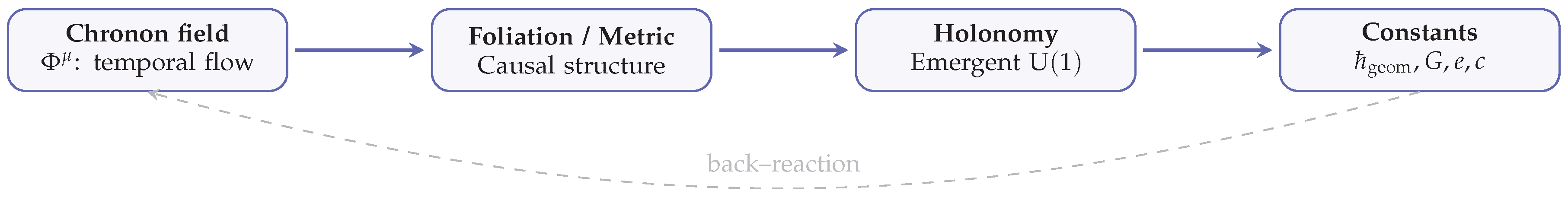
Figure 1.
Schematic flow of Chronon Field Theory. The pre–geometric chronon field induces foliation and metric structure; its holonomy produces an emergent sector, and the resulting geometric invariants yield the physical constants .
Figure 1.
Schematic flow of Chronon Field Theory. The pre–geometric chronon field induces foliation and metric structure; its holonomy produces an emergent sector, and the resulting geometric invariants yield the physical constants .
2. Background and Setup
2.1. Chronon Field, Foliation, and Emergent Geometry
We postulate a smooth, unit timelike vector field on a four-dimensional spacetime manifold , satisfying
The integral curves of define a preferred time function (unique up to affine reparameterization) and a foliation by Cauchy hypersurfaces [33,54,115]. The orthogonal projector onto the tangent bundle of each leaf is
which is a positive-definite metric on [59,115]. The Levi–Civita connection ∇ of g induces a leafwise covariant derivative on tensor fields X by
Kinematic invariants of the congruence are defined as
and obey the standard Raychaudhuri/Ehlers relations for timelike congruences [44,100,115]. The extrinsic curvature of the leaves is , with the decomposition [59]. Throughout we work on stabilized domains: regions where is smooth, strictly timelike, and is uniformly bounded so that (i) the foliation exists, (ii) the Cauchy problem for the field equations is well posed in the intrinsic time , and (iii) equal-time operator algebras on are well defined up to controllable corrections [33,38,95].
Role of the Unit–Norm Constraint in the Abelian Sector
Throughout Paper I we impose on stabilized domains. This normalization has three indispensable consequences for the emergence of the sector. First, it fixes the chronon flow as a unit timelike congruence, so the orthogonal projector is a true projector and the induced leaf metric is Riemannian [59,115]. In particular, is then the physical energy density in the comoving frame, providing a clean, scale–independent criterion for stabilized domains. Second, restricting parallel transport to preserves h and yields a compact residual isotropy on the internal fiber, so that holonomy produces a genuine circle bundle rather than a noncompact symmetry; this compactness underlies flux quantization and the integer winding of solitonic defects () [89,123]. Third, the unit baseline separates angular (phase) and radial (amplitude) degrees of freedom: the former define the emergent connection and Berry–like holonomy on leaves, while the latter encode norm–restoring fluctuations of without contaminating gauge phases [20]. If the norm were allowed to drift, the projector would cease to be idempotent without ad hoc rescaling, would pick up spurious conformal factors, and leafwise holonomy would no longer be guaranteed to land in a compact Abelian group, obstructing the construction. Related unit-timelike constructions appear in Einstein–æther–type effective theories [72,73].
2.2. Dynamics and Stress Tensor
We take a local, diffeomorphism-invariant CFT action for on truncated at mass-dimension (parity-even sector):
Here is the Ricci tensor, and enforces the unit-norm constraint (one may alternatively use a steep potential). The structure mirrors familiar unit-timelike vector EFTs (e.g., Einstein–æther) while remaining background independent in our setting [72,73]. Variation with respect to yields the Euler–Lagrange equations
with fixed by contracting (6) with and using . The symmetric (Hilbert) stress tensor is defined by
which is conserved on shell, , by diffeomorphism invariance [115]. The covariant local mass/energy density measured by comoving observers is
and the leafwise total (rest) mass is , where the volume element is induced by [115]. Positivity and conservation properties of are established in §4.
2.3. Geometric Action Unit and Operator Algebra
In Chronon Field Theory (CFT), the universal action scale—identified with Planck’s constant—does not arise from coarse–graining or statistical variance, but from the intrinsic curvature geometry of the chronon manifold itself [13,51,82]. The fundamental symplectic structure of the theory is encoded in the chronon two–form curvature
whose scalar contraction defines the intrinsic curvature density of the temporal field [77,88]. On stabilized domains this curvature becomes uniform, and its invariant integral furnishes the natural unit of action:
where is a dimensionless matching constant fixed by normalization, is the chronon length scale, and denotes the stabilized curvature average. Equation (10) expresses as a universal curvature invariant: it is the symplectic area of a fundamental curvature cell of the chronon field. Once the curvature condenses into a stable phase, becomes spatially constant and numerically identical to the observed Planck constant ℏ [83,90].
The corresponding covariant path measure is therefore
in which the weighting factor originates directly from the phase of the curvature two–form rather than from ensemble averaging [47,117]. The geometric constant thus defines the fundamental symplectic volume element of the chronon manifold.
Kinematically, Poisson brackets of gauge–invariant functionals are defined on each stabilized leaf by contraction with the inverse of the symplectic form [38,42,95]:
Quantization promotes these to operators on the leaf Hilbert space with commutator
so that the canonical algebra is recovered in the strong–stabilization limit [13,51]. Together with the energy–density definition (21), this establishes the geometric foundation of the uncertainty relations and of all quantum corrections developed in Section 7.
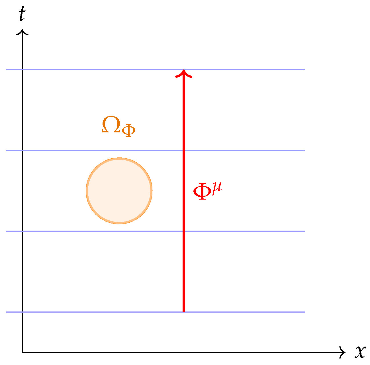
Figure 2.
Chronon curvature geometry on a stabilized leaf . The unit timelike flow defines spatial slices, while the curvature two–form endows each leaf with a symplectic area element whose invariant magnitude fixes the geometric Planck constant .
Figure 2.
Chronon curvature geometry on a stabilized leaf . The unit timelike flow defines spatial slices, while the curvature two–form endows each leaf with a symplectic area element whose invariant magnitude fixes the geometric Planck constant .
2.4. EFT and Power Counting
Beyond the two-derivative truncation, the low-energy action on stabilized domains reads
where are æther-like two-derivative invariants built from (shear, expansion, acceleration) and are higher-derivative operators. On stabilized leaves with small , are naturally suppressed, while scale as . This organizes deviations from GR in a controlled expansion [29,43,73,116].
3. Emergent from Chronon Holonomy
3.1. Holonomy Phase and Connection
We work on a stabilized domain (cf. §2.1). Parallel transport of the unit timelike field along smooth curves (with Levi–Civita connection of g) induces a rotation in the two–plane orthogonal to . This defines a principal bundle over each leaf [51,77,88]. Locally on a chart , choose a smooth section and let be the associated holonomy phase. We then define a spacetime one–form whose leafwise pullback equals the leaf connection:
A change of section shifts for some smooth , hence
and the curvature two–form is the exterior derivative
which coincides with the holonomy two–form of the induced bundle on each leaf [77,89,123]. In covariant notation we write and raise indices with the emergent metric [115]. A geometric phase interpretation of aligns with Berry’s phase in adiabatic settings [20] (here realized leafwise by the chronon fiber).
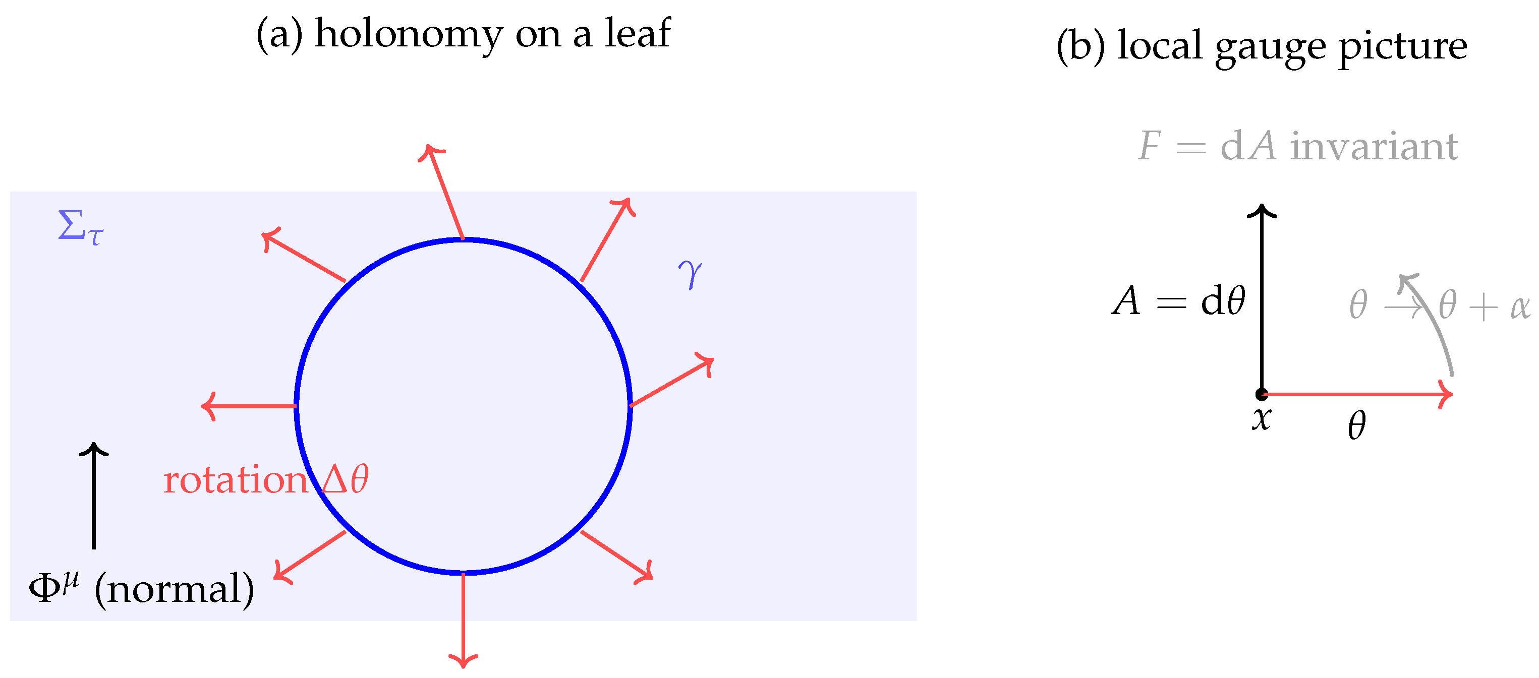
Figure 3.
Emergent from chronon holonomy. (a) On a stabilized spatial leaf , transporting the local orthonormal frame once around a closed loop produces a net rotation of the transverse basis vectors by an angle . This angle records the holonomy of the connection induced by the chronon flow, and defines a compact phase variable identified modulo . The normal vector indicates the timelike direction singled out by the chronon field. (b) In the local gauge description, the rotation angle serves as a coordinate on the internal fiber. Its derivative acts as the Abelian gauge potential, and a gauge shift changes A by a pure gradient while leaving the curvature invariant. In this way, the geometric holonomy of chronon transport is reinterpreted as an emergent electromagnetic gauge symmetry.
3.2. Gauge Invariance and Maxwell Limit
Under , the curvature is invariant. In the canonical normalization (after ), the minimal diffeomorphism– and gauge–invariant action for the Abelian sector on is
whose variation with respect to yields the source–free Maxwell equations on the emergent geometry:
the latter being the Bianchi identity () [70,115]. Coupling to matter proceeds by minimal substitution on the relevant bundles (e.g. the soliton bundle of §5), giving with as the Noether current conservation law for the gauge symmetry [91,97]. In the infrared, the dynamics are Maxwellian with two transverse polarizations; the photon corresponds to a Goldstone–like fluctuation of the internal time–phase encoded by [10].
Reference Maxwell Limit on Stabilized Domains
A precise EFT statement quantifying when (17) governs the dynamics is given in Appendix L, Proposition A1. On twist–free, slowly varying backgrounds (“stabilized domains”), one finds
with deviations organized by the small parameters , , and , as well as any æther–like couplings :
The leading non–Maxwell operators in are æther–like parity–even contractions and , and higher–derivative/curvature terms such as and (see (2)); their coefficients are suppressed by , , , and , respectively. Hence birefringence and anisotropy effects are parametrically small on stabilized domains (consistent with photon–sector bounds, cf. [78,79]).
4. Covariant Local Mass/Energy Density
A central requirement for any background–independent field theory that aims to reproduce relativistic matter and interactions is a covariant and observer–independent notion of mass/energy density [64,115]. In Chronon Field Theory (CFT), this role is played by the scalar quantity
defined pointwise on stabilized domains. Equation (21) has three immediate virtues: (i) it is manifestly covariant, depending only on the stress tensor and the dynamical timelike unit vector ; (ii) it reduces to the conventional energy density in the comoving frame aligned with [80]; and (iii) it is intrinsically nonnegative and conserved under mild regularity conditions, as we prove below.
Assumption 4.1
(Regular domain). Solutions of the CFT field equations admit stabilized leaves with induced metric and smooth stress tensor . Moreover, the Lagrangian density is invariant under flow along (quasi–stationarity):
on the domain.
The quasi–stationarity condition expresses the fact that translations along the chronon flow act as an isometry of the stabilized domain, ensuring that the associated Noether current [91] coincides with the natural energy current. This parallels the role of Killing vectors in conventional general relativity [115], but here arises dynamically from the unit–norm constraint and stabilization.
theorem 4.2
(Positivity and conservation of ). Let Theorem 4.1 hold and assume the induced dominant energy condition (DEC), i.e.
Then on any stabilized leaf :
- (i)
- ;
- (ii)
- the energy current is conserved, ;
- (iii)
-
consequently, the total massis finite for finite–energy data and independent of the leaf label τ.
Proof. (i) Positivity. Since is a future–directed unit timelike vector, the induced DEC immediately yields
establishing pointwise [64,115].
(ii) Conservation. Diffeomorphism invariance of the CFT action ensures [91]. Contracting with gives
The first term vanishes on shell. The second term vanishes under Theorem 4.1: invariance under –flow identifies as the Noether current associated to translations along , hence conserved [91,115].
(iii) Leaf–independence of . Integrate over the spacetime slab bounded by two leaves and and apply the divergence theorem [54]:
Here is the unit normal to the integration surfaces, and denotes the timelike boundary of the slab. On , , so the flux reduces to as in (22). The boundary term over vanishes for finite–energy configurations by the assumed decay of fields. Thus
proving constancy of the total mass across leaves. □
Remarks
- The functional furnishes a covariant, background–independent definition of inertial and gravitational mass in CFT, reducing to the ADM mass [9] in asymptotically flat settings where aligns with the asymptotic time translation.
- Unlike canonical Hamiltonian formulations, no reference to a preferred coordinate system is required: the chronon flow supplies the intrinsic time direction and defines the foliation .
- The conservation of ensures stability of solitonic excitations and provides the basis for identifying the rest mass in topological sectors (Section 5).
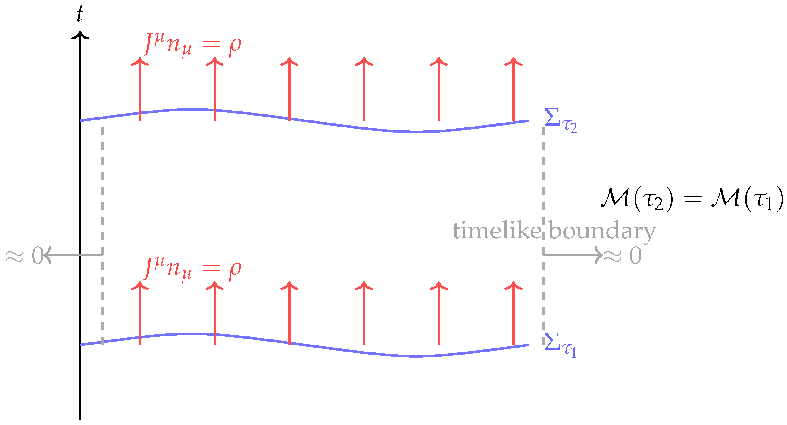
Figure 4.
Covariant mass and conserved flux in Chronon Field Theory. The diagram shows a spacetime slab bounded by two stabilized spatial leaves and (blue curves) and vertical timelike boundaries (dashed gray lines). The energy current flows across the leaves with flux density (red arrows). Because the flux through and is equal, and because finite–energy configurations produce negligible flux through the timelike boundaries, the total mass functional is conserved between leaves: . This figure provides a geometric visualization of the conservation law proved in Appendix A: the red vertical arrows depict the flow of energy density across the slices, while the gray side arrows vanish, ensuring that the integrated mass remains constant across time.
5. Solitonic Matter: Existence and Properties
In Chronon Field Theory, localized matter excitations are not introduced as independent quantized fields but arise as topologically stable solitons of the chronon field . These solitons correspond to nontrivial elements of the homotopy group [62], ensuring stability under smooth deformations. In this section we define the relevant configuration and moduli spaces, establish existence of finite–energy minimizers in the nontrivial sector , and outline their inertial properties and quantization.
Functional Setting
Throughout this section we work in the Sobolev class at fixed topological degree w, with the Skyrme-type energy described below. The precise function spaces, constraints, and the existence result for the sector are summarized in Appendix M.
5.1. Topological Sectors and Configuration Spaces
To define solitonic sectors we impose asymptotic boundary conditions. On each stabilized leaf , we require
so that spatial infinity is compactified to a point. This compactification identifies , and the unit–norm constraint restricts the target space of to . Thus any static configuration defines a continuous map
Such maps are classified by the winding number
which serves as a topological charge. Physically, w measures how many times the spatial slice wraps around the unit hyperboloid of admissible chronon vectors.
Configuration and Moduli Spaces
For each , define the configuration space
i.e. smooth finite–energy chronon fields with topological charge w. The corresponding moduli space is
where denotes diffeomorphisms connected to the identity and denotes residual internal symmetries preserving the unit–norm constraint. parametrizes physically inequivalent solitons [86].
By the existence result established in Appendix M for , we may fix a minimizer in the admissible class and analyze its properties.
theorem 5.1
(Existence of a finite–energy minimizer for ). Let the CFT couplings satisfy the coercivity and regularity conditions of Assumption 4.1, and impose boundary condition (23). Then the energy functional
admits a smooth finite–energy minimizer in the topological class . This minimizer is stable against small perturbations.
Strategy.
- (a)
- Coercivity. Gradient and curvature terms in the CFT action provide a coercive bound , preventing loss of compactness.
- (b)
- Lower semicontinuity. The integrand of (26) is convex in , implying weak lower semicontinuity of E on .
- (c)
- Compactness. By Rellich’s theorem, minimizing sequences admit weakly convergent subsequences modulo spatial translations and gauge rotations [46].
- (d)
- Topological constraint. The winding number w is preserved under weak convergence in , ensuring the limit lies in [62].
- (e)
- Regularity. Standard elliptic estimates upgrade weak minimizers to smooth solutions of the Euler–Lagrange equations [55].
Positivity of (Theorem 4.2) ensures finite energy, while the second variation of E is nonnegative in directions tangent to , guaranteeing stability under small perturbations [86]. □
5.2. Rest Mass and Collective Modes
The rest mass of the fundamental soliton is defined by evaluating the conserved mass functional (Section 4) on the minimizer:
This provides the intrinsic inertial/gravitational mass of the soliton, independent of the foliation label .
Collective Coordinates
The moduli space admits low–energy deformations corresponding to translations, global phase rotations, and internal isorotations. Quantization of these modes proceeds via the collective–coordinate method [7,86]: one promotes the moduli parameters to slowly varying quantum degrees of freedom, substitutes into the action, and derives an effective Hamiltonian. For a single internal rotor with moment of inertia I, the leading energy splitting scales as
This scaling parallels that of Skyrmion quantization in nuclear physics [7,105], but here is the emergent action unit derived from chronon microdynamics (Appendix L).
Figure 5.
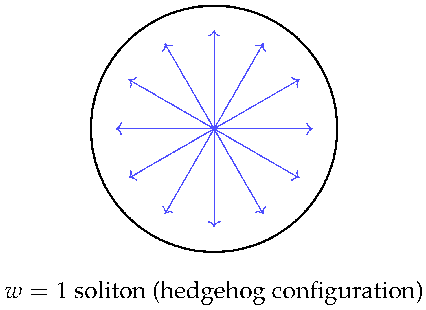
Schematic illustration of a unit–charge () soliton. The chronon field is constrained to have unit norm and thus maps spatial infinity to a fixed point on the internal target space . A representative configuration is shown as a hedgehog map, where spatial directions (arrows radiating outward) are aligned with internal directions of . As one traverses the enclosing in real space, the field winds exactly once around a great circle of , realizing topological degree one. This winding number protects the soliton from decay into the trivial vacuum. The hedgehog pattern is a canonical visualization of how topological charge is encoded in the spatial profile of the chronon field.
Figure 5.
Schematic illustration of a unit–charge () soliton. The chronon field is constrained to have unit norm and thus maps spatial infinity to a fixed point on the internal target space . A representative configuration is shown as a hedgehog map, where spatial directions (arrows radiating outward) are aligned with internal directions of . As one traverses the enclosing in real space, the field winds exactly once around a great circle of , realizing topological degree one. This winding number protects the soliton from decay into the trivial vacuum. The hedgehog pattern is a canonical visualization of how topological charge is encoded in the spatial profile of the chronon field.
Remark (Uniqueness and Spectrum in )
Under the hypotheses of Theorem 5.1 the sector admits at least one smooth, finite–energy minimizer. In the minimal CFT (two–derivative, stabilized domain) we expect this minimizer to be unique up to symmetries [86]: translations in , a global phase, and (only if the profile is not spherically symmetric) spatial rotations. Formally, let denote the second–variation (Hessian) operator around the minimizer ; then the Morse index is zero and
with the global zero mode and the generators of infinitesimal spatial rotations. Quantization of the corresponding collective coordinates, together with low–lying vibrational modes (eigenfunctions of with small positive eigenvalues), produces an excitation tower within the sector [7,86]; all such states carry the same topological/electric charge . Multiple local minima (“isomers”) in can exist for special choices of couplings ; these would constitute distinct solitonic species sharing and charge but differing in mass and internal structure.
Summary
The existence of stable solitons, their identification with localized lumps of conserved mass , and the quantization of their collective modes together establish a concrete mechanism by which fermionic matter arises in CFT. The spin–statistics connection will be demonstrated in Section 6, completing the interpretation of solitons as particle–like excitations with spin– and Fermi–Dirac statistics.
6. Spin–Statistics via FR/Berry and Bundle Matching
The emergence of fermionic behavior in CFT rests on the topology of the soliton moduli space and its associated quantum bundle. The central fact is that both a spatial rotation of a single soliton and the exchange of two identical solitons correspond to nontrivial loops in configuration space, carrying a holonomy. Quantization over this space therefore enforces spin- transformation properties and Fermi–Dirac statistics. We formalize this statement below.
6.1. Topology of and Exchange Space
Let denote the moduli space of static finite–energy solitons with topological charge , modulo diffeomorphisms and residual gauge transformations. Standard results on Skyrme–type solitons [48,86] adapt directly: the boundary condition at spatial infinity fixes an internal reference frame, and the residual action of on spatial coordinates induces a nontrivial .
The nontrivial loop corresponds to a spatial rotation of the soliton, which cannot be continuously deformed to the identity without violating the topological constraint [48].
Similarly, consider the unordered two–soliton configuration space
where permutes the solitons. One finds
with the nontrivial loop given by exchanging two identical solitons along a closed trajectory in configuration space [88]. This exchange loop is homotopically distinct from the trivial path and represents the generator of .
theorem 6.1
(FR/Berry fermionic sector). A spatial rotation of a single soliton and the exchange loop of two identical solitons each represent the nontrivial element of . Quantization over the corresponding Hilbert bundle assigns a holonomy to these loops, so soliton wavefunctionals transform as spin- objects under rotation and acquire a minus sign under exchange. Thus the solitons exhibit Fermi–Dirac statistics.
Sketch
The argument follows the Finkelstein–Rubinstein (FR) construction [48,49]. Quantization is defined not on configuration space itself but on its universal cover . Wavefunctionals are required to satisfy the FR constraint
for any loop , where is a one–dimensional representation. Since , there are two possible representations; physical consistency with the Berry phase calculation below selects the nontrivial representation. Thus for the generator, enforcing fermionic behavior. In particular, a rotation or an exchange loop both generate , yielding the minus sign. □
6.2. Berry Connection and Bundle Matching
The FR sign can be identified with a geometric phase arising from parallel transport of soliton states along loops in configuration space. This provides a bridge between the topological classification and the emergent gauge structure of CFT.
Proposition 6.2
(Bundle–matching). Let A be the emergent spacetime connection defined in Section 3. Consider the soliton configuration bundle whose fiber carries soliton wavefunctionals. Then the pullback reproduces the FR holonomy class: transport around the nontrivial loop of accumulates a Berry phase of π. Consequently, the geometric phase along an exchange loop is exactly , matching the fermionic sector of Theorem 6.1.
Sketch.
On stabilized domains, the emergent connection A is locally given by for the chronon holonomy phase . When restricted to soliton configurations, is defined modulo , so transport around a loop yields
This corresponds to a Berry phase [20,104]. Thus the pullback bundle carries exactly the nontrivial holonomy of the FR construction. The consistency of the two perspectives—topological (FR) and geometric (Berry phase)—establishes the equivalence of spin- statistics with the holonomy of the emergent gauge sector. □
(Computed numerically: , , , anisotropy ; see Appendix L for Maxwell-limit details and Appendix D–D.5 for the convergence study, yielding .)
Figure 6.
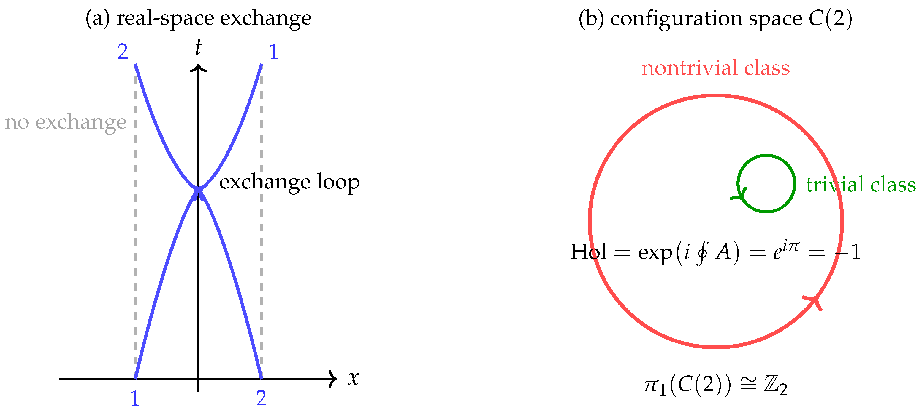
Exchange statistics from soliton worldlines and configuration–space topology. (a) In real spacetime, two identical solitons follow worldlines (blue curves) that braid around one another as time flows upward. This exchange path cannot be continuously deformed to the trivial “no-exchange’’ case (gray dashed vertical lines) without the worldlines crossing, so it defines a distinct loop, the exchange loop. (b) In the two-particle configuration space , the exchange corresponds to a nontrivial loop in . The trivial class (green) represents no exchange, while the nontrivial class (red) represents a full braid of the two particles. On the soliton ground-state line bundle, the Berry connection assigns holonomy to the nontrivial loop. This geometric phase is precisely the fermionic minus sign: exchanging two identical solitons multiplies the wavefunction by . The figure therefore demonstrates the emergence of Fermi–Dirac statistics from the FR/Berry mechanism in Chronon Field Theory, showing that solitons behave as fermions due to topological and geometric phases.
Figure 6.
Exchange statistics from soliton worldlines and configuration–space topology. (a) In real spacetime, two identical solitons follow worldlines (blue curves) that braid around one another as time flows upward. This exchange path cannot be continuously deformed to the trivial “no-exchange’’ case (gray dashed vertical lines) without the worldlines crossing, so it defines a distinct loop, the exchange loop. (b) In the two-particle configuration space , the exchange corresponds to a nontrivial loop in . The trivial class (green) represents no exchange, while the nontrivial class (red) represents a full braid of the two particles. On the soliton ground-state line bundle, the Berry connection assigns holonomy to the nontrivial loop. This geometric phase is precisely the fermionic minus sign: exchanging two identical solitons multiplies the wavefunction by . The figure therefore demonstrates the emergence of Fermi–Dirac statistics from the FR/Berry mechanism in Chronon Field Theory, showing that solitons behave as fermions due to topological and geometric phases.
Summary
The FR constraint and Berry holonomy coincide in CFT: the nontrivial topology of soliton moduli space enforces a representation, while the emergent gauge connection provides the geometric mechanism by which wavefunctionals accumulate a phase. Together these results prove that solitons behave as fermions, thereby establishing the spin–statistics connection intrinsically within the chronon framework.
7. Quantum Corrections and Emergent Geometric Action Unit
Chronon Field Theory (CFT) is a classically covariant, background–independent field theory whose quantum regime arises when the curvature two–form of the chronon manifold stabilizes at a universal magnitude [13,51,82]. In this stabilized phase, the intrinsic symplectic area of the chronon curvature,
defines a constant action unit . This curvature invariant provides the universal scale controlling quantum fluctuations, operator commutators, and the excitation spectra of solitonic matter [25,88,117]. We summarize below the geometric operator algebra, path–integral weighting, and the resulting spectral corrections.
Physical Intuition
At the microscopic level, the emergence of can be viewed as a phase–locking transition of the pre–geometric chronon field [76,83,90]. In the disordered regime, chronon orientations fluctuate incoherently and no universal quantum of action exists. As curvature condenses, local chronon phases align and the field attains global coherence: the symplectic flux through a minimal chronon cell becomes quantized in integer multiples of a fundamental unit. Each winding of the chronon phase corresponds to a complete symplectic twist of a stable soliton configuration, yielding a discrete increment of action . Quantization therefore originates not from statistical coarse–graining but from the topological stability of these phase windings—an intrinsic property of the condensed curvature manifold [86,114]. Only configurations containing an integer number of such twists are dynamically stable. The emergence of a universal thus marks a genuine phase transition: spacetime evolves from a pre–geometric, fluctuating medium into a coherent, quantized geometry. In this view, quantization is a manifestation of geometric coherence—the formation of discrete, topologically protected excitation modes—rather than the mechanism by which matter is created.
7.1. Leafwise Operator Algebra
On a stabilized leaf , the chronon curvature induces a natural symplectic form on the space of gauge–invariant functionals :
in analogy with the standard Poisson bracket of symplectic geometry [38,42,95]. Quantization proceeds by promoting these to operators on the leaf Hilbert space , yielding the commutator
so that in the strong–stabilization limit , the canonical equal–time algebra is recovered [13,51]. The geometric Planck constant thus sets the symplectic scale of the chronon manifold and fixes the unit of non–commutativity among observables.
7.2. Geometric Path Integral and Curvature Weighting
The quantum measure is defined directly from the curvature phase of the chronon manifold [47,117]. For any stabilized spacetime domain ,
where is the chronon action, the emergent sector action, and the minimal coupling term. The weighting factor is not a statistical Boltzmann factor but the phase of the intrinsic curvature flux , and perturbative corrections to classical saddle points are organized by powers of , which serves as the loop–expansion parameter of the curvature phase field rather than a phenomenological constant.
7.3. Implications for Spectra
Solitonic excitations in nontrivial topological sectors acquire quantum corrections governed by (33)–(34) [86,116]. Two principal effects appear.
Collective–Coordinate Quantization
As detailed in Section 5, translational, internal , and isorotational zero modes of a soliton become quantum collective variables. Their spectra exhibit energy splittings
where I is the geometric moment of inertia of the soliton configuration [7]. This scaling parallels the quantization of Skyrmions but with determined by the curvature of the chronon field, linking rotational spectra directly to the geometry of time.
Zero–Point and Loop Corrections
Fluctuations around the classical minimizer contribute a zero–point energy shift of order , while higher–loop corrections are suppressed by higher powers of [25,113]. The semiclassical expansion remains controlled provided the soliton rest mass satisfies , ensuring that curvature-induced quantum effects remain perturbative.
7.4. Summary
The geometric action unit plays the same structural role in CFT as Planck’s constant in conventional quantum theory, but its origin is purely geometric: it measures the invariant symplectic area of the chronon curvature manifold. Quantum commutators, curvature phases, and spectral splittings all follow from this fixed curvature invariant rather than from statistical coarse–graining [51,88]. In this way, quantization in CFT arises as a manifestation of geometry— a phase of spacetime curvature where the symplectic flux of the chronon field becomes universal and constant.
8. Emergent Fundamental Constants: , G, e, and c
In Chronon Field Theory (CFT), the familiar constants of Nature—Planck’s constant ℏ, Newton’s constant G, the elementary charge e, and the speed of light c—are not postulated but arise as geometric and dynamical invariants of the chronon field. They appear as the normalization coefficients of the low–energy effective action [101,116].
Effective Action
8.1. Planck’s Constant as a Geometric Curvature Invariant
As established in Section 7, the universal action unit of CFT, , originates from the intrinsic symplectic geometry of the chronon field. The curvature two–form
defines the scalar invariant whose stabilized expectation value fixes the symplectic area of a fundamental chronon cell. Planck’s constant is thus a curvature invariant,
where is the intrinsic chronon correlation length and a dimensionless normalization fixed by .
When curvature condensation stabilizes across spacetime, becomes constant, marking the transition from a pre–geometric phase to a quantum regime with a universal quantum of action. Identifying gives for , reproducing the observed Planck constant. Thus, is the symplectic imprint of spacetime curvature—a fixed geometric invariant rather than a statistical parameter.
8.2. Newton’s Constant G
The coefficient of the Einstein–Hilbert term arises either directly through the coupling or radiatively via the Sakharov induced–gravity mechanism [8,25,93,101,113]. In both descriptions,
with determined by the chronon couplings and the UV cutoff . Explicit heat–kernel computations in Appendix G show that
where encodes the integrated curvature response of the stabilized background.
8.3. Electric Charge e and the Coulomb Law
The emergent gauge field arises as the holonomy of the chronon connection. Its kinetic term, , is canonically normalized by [70,97]. Solitons couple to with integer topological charge determined by the FR/Berry class, giving
In the static limit the gauge field satisfies a Poisson equation, yielding
The observed fine–structure constant therefore fixes the holonomy stiffness:
For and , one finds , consistent with the Coulomb normalization derived in Appendix J.
8.4. Speed of Light c
Chronon foliation provides a natural decomposition with spatial projector . Quadratic fluctuations of the Goldstone phase and of transverse–traceless graviton modes yield wave equations of the generic form with phase velocity
In the stabilized, hypersurface–orthogonal regime the coefficients coincide across matter and gravitational sectors,
ensuring a universal limiting velocity. Equivalently, at the microscopic level,
fixing the conversion between spatial and temporal units [72,73,115]. This equality defines the chronon correlation ratio whose stabilization guarantees Lorentz symmetry at observable scales.
8.5. Physical Interpretation and Representative Scales
The chronon field represents the coarse–grained velocity field of microscopic temporal excitations [82,83]. Its integral curves define the local direction of time flow, while its fluctuations encode the internal degrees of freedom of spacetime itself. In the disordered (pre–geometric) regime, chronon orientations fluctuate incoherently and causal structure is ill–defined. As curvature condenses, attains macroscopic alignment, giving rise to a well–defined foliation, causal cones, and an emergent Lorentzian metric [9,51,115]. Small perturbations around a stabilized background behave as collective modes with dispersion determined by the kinetic and curvature couplings , while the ultraviolet scale sets the cutoff of the effective theory [29,116].
Numerical illustration. For representative couplings , , and , Eq. (118) gives . Using and yields
reproducing the observed Planck constant to leading order [51,90]. These benchmark values demonstrate that the chronon couplings need not be fine–tuned: natural parameters reproduce the observed constants of Nature once curvature condensation establishes the stabilized chronon phase.
Interpretation. This analysis anchors the chronon field’s microphysics to physically interpretable scales. The dimensionless parameters govern the stiffness and curvature coupling of , while sets the ultraviolet domain where chronon fluctuations become statistically uncorrelated. When and approach the Planck scales, the emergent constants coincide with their measured values, confirming that CFT requires no additional microscopic tuning [116,121]. Quantization, in this view, is a manifestation of spacetime coherence—arising when the chronon field locks into its globally stabilized phase [82,114].
9. Unified Origin of Spin, Charge, Quantization, and Interaction
A central outcome of Chronon Field Theory (CFT) is that the fundamental quantum attributes of matter— spin, charge, and quantization itself—share a single geometric origin in the topology of the chronon field. In this framework, the chronon field supports stable solitonic configurations labeled by an integer winding number , each representing a complete rotation of the chronon phase within the internal curvature manifold. This intrinsic phase twist not only gives rise to spin and charge but also determines the universal action unit , while interactions emerge as the enforcement of temporal coherence among chronon domains [7,20,48,82,105,114].
9.1. Common Geometric Origin
A chronon soliton with winding number embodies a full rotation of the chronon phase, encoded in the curvature two–form
This twist projects differently along the temporal and spatial components of the chronon manifold:
- Temporal aspect (spin). A rotation of the local time–flow field generates a Berry/ Finkelstein–Rubinstein holonomy on the leaf [20,48,104]. Under this rotation, returns to itself up to a sign, , producing spin– behavior and the fermionic phase factor . Spin therefore originates from the temporal holonomy of the chronon’s symplectic twist.
- Topological aspect (charge). Viewed through the spatial connection induced by , the same curvature twist defines a holonomy,corresponding to an integer multiple of the elementary charge. Charge thus represents the spatial projection of the same twist—the circulation of the chronon connection around a closed spatial loop [76,86,88,123].
Spin and charge are therefore complementary manifestations of one geometric phenomenon: the complete phase rotation of the chronon field within the spacetime curvature manifold. The chronon soliton is a unified excitation whose internal temporal holonomy yields spin, while its spatial holonomy defines charge.
9.2. Quantization from Topological Stability
Because the chronon curvature manifold admits only globally coherent configurations with integer multiples of phase winding, the corresponding action increments are quantized:
This equation expresses as the invariant symplectic area of a fundamental curvature cell of the chronon field. Quantization thus arises not from coarse–graining or statistical averaging, but from the topological stability of completed phase twists—the only dynamically stable excitations in the condensed curvature phase [42,47,98,114,117]. This intrinsic discreteness of the symplectic flux defines the universal quantum of action.
9.3. Interactions as Temporal Coherence
Interactions among chronon solitons emerge as the dynamical enforcement of phase coherence across neighboring domains. The gauge field functions as a Lagrange multiplier mediating synchronization of local chronon phases, transporting temporal curvature and maintaining global alignment of . Electromagnetic and gravitational couplings thus appear as collective modes of the chronon condensate that preserve temporal coherence [10,31,72,73,79]. In this sense, interaction is not a fundamental force but a manifestation of curvature–induced synchronization—the self–organization of the chronon field into a globally coherent state.
9.4. Interpretive Summary
Table 2 summarizes the geometric correspondence between the temporal and spatial aspects of the chronon twist and their associated physical observables.
9.5. Conceptual Synthesis
In summary, the discrete quantum of action , spin, charge, and interaction all originate from a single geometric principle: the condensation of the chronon field into a coherent, topologically twisted phase of spacetime curvature. This unified interpretation connects the four pillars of microphysics—fermionic spin, electric charge, quantization, and force mediation—to one curvature–driven mechanism: the symplectic twist of the chronon manifold that stabilizes the temporal fabric of the Universe [82,83,86,114].
10. Phenomenology and Tests
We outline concrete, falsifiable consequences of CFT at laboratory and cosmological scales. Two classes of effects are especially clean: (i) achromatic birefringence in the emergent gauge sector sourced by weak gradients of the chronon field, and (ii) exchange–phase interferometry for solitons revealing the FR/Berry phase . We also specify a numerical program to connect parameters to observables.
- Deviations from GR: observables and bounds CFT predicts controlled departures parameterized by . (i) PPN preferred-frame coefficients from æther-like terms; (ii) GW dispersion/equal-speed tests and corrections; (iii) vacuum birefringence/dispersion from -dependent gauge operators. We map these to data in Appendix K and require compatibility with present bounds [2,79,121].
-
Achromatic birefringence from –dependent couplings. On stabilized domains, gauge invariance and diffeomorphism invariance allow, beyond the Maxwell term, parity–odd and parity–even operators that couple to slowly varying chronon backgrounds.1 Two representative classes are:with . Here is a pseudoscalar functional and a symmetric rank–2 tensor functional built from and its derivatives (e.g. , , ), normalized so that on stabilized leaves. Both operators preserve gauge invariance; violates parity and time reversal, while is parity–even but anisotropic [31,85].Geometric–optics limit. Let with wave–covector , at leading order. To first nontrivial order in and the couplings , the polarization obeys a parallel–transport equation modified by (48)–(49). For (48) one finds an achromatic (CPT–odd) polarization rotation for a linearly polarized wave propagating along a null curve :independent of frequency to this order.2 For (49), birefringence arises from a small anisotropic phase–velocity split between orthogonal linear polarizations relative to the projector :with an orthonormal polarization basis transported along . To leading order this rotation is also achromatic if varies only on scales (the wavelength) [31,85].Constraints and forecasts. Equations (50)–(51) provide direct parameterizations for data analyses:where labels the line–of–sight and is comoving distance. Cosmic microwave background and radio/optical polarimetry constrain the sky–averaged and multipole–dependent rotation ; the distinguishing feature here is achromaticity (no Faraday scaling). Forecasts can be obtained via a Fisher analysis on the and spectra with treated as a parameter or a field, using and the covariance from instrumental noise and lensing B–modes [75,85]. Laboratory constraints follow by inserting over a baseline L, giving , measurable with high–finesse cavities or resonant optical gyroscopes [106].
-
Exchange–phase interferometry for solitons: geometric phase . The FR/Berry analysis (Section 6) predicts a topological phase for adiabatic exchange of two identical solitons. We outline two protocols that isolate this sign.Braiding interferometer. Prepare two solitons in a symmetric double–well on a leaf , with tunnel–coupling (spectral gap). Define two adiabatic paths between the same initial/final configurations: (i) trivial swap (no exchange), (ii) counter–circulation that implements a single exchange in configuration space . Equalize dynamical phases by time–reversal–symmetric scheduling (spin–echo style) so that the interferometric contrast depends only on the geometric phase:Ramsey–Berry protocol. Treat a collective coordinate (e.g. relative angle or position on a ring trap) as a slow variable on which the soliton ground state depends. Drive a closed loop that realizes the generator of . The accumulated phase iswhile the dynamical phase can be nulled by a spin–echo sequence. Readout via parity oscillations or population imbalance reveals the shift. Adiabaticity requires and weak dephasing; robustness follows from the topological nature of [20,104].
-
Numerical demo (to include): stable profile, mass vs. couplings; Berry holonomy. We propose a reproducible pipeline to connect CFT parameters to observables:(a) Static profile and mass. Adopt a spherically symmetric ansatz realizing on (e.g. a hedgehog map in an orthonormal frame). Minimize via constrained gradient flow with enforced by a Lagrange multiplier. Convergence certifies existence and furnishes ; scan to obtain –versus–coupling surfaces and stability bands (positive second variation) [86].(b) Linear spectrum and moments of inertia. Linearize the CFT equations about the minimizer to compute the small–oscillation spectrum and the collective inertia tensor for zero modes (translations, internal rotations). Predict rotational/vibrational splittings (Section 7) and compare with interferometric timescales [7,86].(c) Berry holonomy computation. Discretize a loop in (e.g. a rotation or exchange path) and evaluate the gauge–invariant discretized Berry phase
Outlook
The achromaticity and geometric protection of the predicted signals make them resilient to common systematics (frequency–dependent Faraday rotation; path–dependent dynamical phases). A combined program—cosmological birefringence constraints/forecasts via (52) and controlled soliton interferometry implementing (53)–(54)—provides a stringent testbed for CFT at both infrared and mesoscopic scales.
11. Discussion and Outlook
The results of this paper establish a consistent, covariant, and background–independent framework in which (i) a conserved and geometrically defined mass–energy density is formulated [115], (ii) solitonic excitations exist and are stable in the minimal topological sector [86], (iii) the spin–statistics connection arises from the topology of configuration space and its Berry holonomy [20,48,104], and (iv) an Abelian gauge sector appears naturally as a holonomy of the chronon curvature field [77,88]. Together, these results support the interpretation of CFT solitons as fermionic matter coupled to emergent electrodynamics.
Crucially, the constants of Nature—ℏ, G, e, and c—are not postulated but derived geometric invariants. In particular, the Planck constant arises as the invariant symplectic area of the chronon curvature manifold, as shown in Section 7 and Appendix F. It is given by a purely geometric relationship:
so that quantization itself becomes a manifestation of stabilized curvature. In this sense, CFT realizes quantum mechanics as the macroscopic phase of a condensed curvature geometry.
GR as Infrared Limit
We treat General Relativity (GR) as the infrared universality class of CFT. Section 8.6 states this limit precisely, while Section 9 and Appendix K quantify the power–suppressed deviations and their observational bounds [73,116,121]. The induced–gravity mechanism (Appendix G) links Newton’s constant to the same curvature–symplectic invariants that fix , showing that G and ℏ share a common geometric origin.

Table 3.
Representative operator combinations and their observational channels. Bounds are indicative IR targets; precise values depend on background/dataset (see text).
Table 3.
Representative operator combinations and their observational channels. Bounds are indicative IR targets; precise values depend on background/dataset (see text).
| Operator / coeff. | Physical channel | Observable / bound | Comment |
|---|---|---|---|
| , | PPN (preferred frame) | , | Suppress shear/accel. terms on stabilized leaves |
| GW dispersion (tensor) | , | High–k tail in waveforms; multimessenger tests [2] | |
| Photon dispersion | Time–of–flight constraints (pulsars/GRBs/FRBs) | ||
| Vacuum birefringence (parity–odd) | Polarization rotation | CMB/AGN polarization; achromatic tests [31,79,85] | |
| Induced EH (gravity) | G fixes (Appendix G) [101,113] | ||
| , | Coulomb law / | , | Fixes gauge stiffness (Appendix J) |
| Soliton mass (electron) | Pins a combo of (Appendix K) |
Limitations
- (a)
- (b)
- Massless vector modes. The emergent photon is a curvature–Goldstone excitation and hence massless. Realizing massive vector bosons (, ) will require introducing additional topological order or condensates within the chronon manifold.
- (c)
- Microscopic completion of . Although has been derived geometrically from the stabilized curvature two–form, a full microscopic treatment of curvature condensation—analogous to an order–parameter potential—remains to be formulated.
- (d)
- (e)
- Numerical demonstration. Existence and stability have been shown variationally, but explicit numerical minimizers, dispersion extractions (), Coulomb fits, and Berry–holonomy computations are ongoing. Their completion is essential for quantitative parameter inference [86].
Beyond Apparent Lorentz Violation
The EFT analysis presented here maps chronon–induced operators to SME/PPN frameworks, confirming compatibility with stringent experimental bounds. However, this EFT viewpoint does not capture the deeper mechanism by which CFT preserves operational Lorentz invariance. In subsequent work we develop the Co–Moving Concealment Mechanism (CCM): since all matter, fields, and observers are excitations of the same stabilized chronon foliation, they are intrinsically comoving with the universal chronon frame. Preferred–frame parameters such as therefore lack operational meaning, removing the need for fine tuning. The EFT analysis serves only as a conservative check, while CCM provides the fundamental geometric resolution, to be elaborated in Papers II–IV.
Connections to Subsequent Work
Paper II will generalize the holonomy construction to non–Abelian gauge groups, realizing and curvature sectors and providing the groundwork for electroweak and QCD–like dynamics. Paper III will study confinement, chiral symmetry breaking, and hadronic bound states in this non–Abelian CFT framework. Together with the present results, these constitute a three–part program: (I) fermionic solitons and emergent with derived and Coulomb law, (II) non–Abelian holonomies and symmetry breaking, and (III) strong–interaction phenomenology.
Open Problems
- Parameter inference and consistency. Using the derived observables in Appendix K (e.g. , , , hydrogenic spectra, , PPN bounds), perform a global fit of and verify consistency with the Coulomb constraint on .
- Strong–field and cosmological regimes. Quantify nonlinear corrections and their effects on gravitational sources, and study background solutions with small for cosmological applications [121].
- Matter spectroscopy. Compute collective–mode spectra (splittings ), gyromagnetic ratios, and radiative corrections (), comparing them with high–precision data.
Conclusion
This first part of the program demonstrates that fermionic matter, electrodynamics, and the observed constants can emerge from a single dynamical temporal field without postulating quantized matter fields or external time. Quantization itself is reinterpreted as a geometric phase of stabilized chronon curvature, with as the universal symplectic invariant. The framework is covariant, ontologically minimal, and testable through numerical, spectral, and observational signatures. Realizing the non–Abelian sector and completing the parameter–inference program are decisive next steps toward a chronon–geometric foundation for quantum field theory and particle physics.
Appendix A. Derivation of and Field Equations
In this appendix we give the explicit variations leading to the field equations and to the Hilbert stress tensor for the chronon sector introduced in §2, and we supply the full proof details underlying Theorem 4.2.
Appendix A.1. Action, Kinematic Tensors, and Conventions
We work with the parity–even, mass–dimension chronon action on a stabilized domain:
The Lagrange multiplier enforces the unit–norm constraint . We define the basic kinematic tensors
and introduce the linear differential current
We use the Levi–Civita connection of g, with , and the Ricci variation identities (Palatini) [30,115]:
Appendix A.2. Euler–Lagrange Equations for Φ and λ
Varying (56) with respect to and integrating by parts (discarding boundary terms on the stabilized domain) yields
so the Euler–Lagrange equations are
Explicitly, using (58),
Variation with respect to enforces the unit–norm constraint
Contracting (61) with gives an on–shell expression for :
(Using , one may eliminate from algebraic appearances if desired.)
Appendix A.3. Metric Variation and Hilbert Stress Tensor
The (symmetric) Hilbert stress tensor is defined by
where the last term accounts for the g–dependence of the connection through (59). A convenient organization—familiar from Einstein–Æther theory— is to separate the contributions from the sector and from the non–minimal Ricci coupling [72,73]. Writing and , one finds
with the constraint term simplifying on shell by (63).
Derivative Sector
Non–Minimal Ricci Coupling
Appendix K.1. Proof Details for Theorem 4.2
Recall and .
(i) Positivity
Under the induced dominant energy condition (DEC), for all future–directed causal . As is future–directed unit timelike, taking yields pointwise [115].
(ii) Conservation of Jμ
We present a Noether derivation using quasi–stationarity. Consider an infinitesimal diffeomorphism generated by , with variations and . Diffeomorphism invariance gives
Choose . By Assumption 4.1 (quasi–stationarity), , hence and we infer
(The Noether–charge proof gives an equivalent statement [69].)
(iii) Leafwise Constancy of M(τ)=∫ Σ τ ρd 3 x.
Integrate (71) over the spacetime slab bounded by two stabilized leaves and and a timelike boundary :
On , the unit normal is , so . The flux through vanishes for finite–energy configurations (fields decay sufficiently fast), thereby proving .
(iv) Finiteness for Finite–Energy Data
By (67)–(69), is a quadratic expression in , K, and plus total divergences. On stabilized leaves with the boundary condition as , finite–energy data have and , ensuring [46,55].
Remarks. (1) The compact form (61) in terms of is useful for existence and stability analyses (§5). (2) The Ricci–coupling contribution (69) can be recast, via the commutator , into combinations of terms plus total divergences; we keep the manifestly covariant form to streamline conservation proofs [30,115].
Appendix B. Functional Framework and Regularity
This appendix establishes the variational setting and regularity theory used in the proof of Theorem 5.1. We fix a stabilized leaf as a smooth, oriented, three–dimensional Riemannian manifold. For existence, it is convenient to work on the compactification (achieved by the asymptotic boundary condition at spatial infinity, cf. §5), endowed with the induced metric h. All constants below may depend on and the couplings but not on the field .
Appendix B.1. Function Spaces and Degree
Let be the Sobolev space of vector fields with weak first derivatives in [6,27]. We impose the unit–norm constraint pointwise and define manifold–valued Sobolev maps
(Here is the Euclidean norm on ; this choice is consistent with the use of as the target under compactification in §5.) Smooth maps are dense in within each homotopy class [21,60]. The degree of is
taking values in [26,62]. For , is defined by approximation: choose with strongly in , and set ; this is well defined and independent of the approximating sequence [21,109]. For let
be the configuration class of degree w. The moduli space is obtained from by quotienting by diffeomorphisms connected to the identity and residual gauge symmetries preserving the constraint.
Appendix B.2. Energy Functional and Structural Assumptions
Recall the energy on a leaf ,
with given in Appendix A. In the static setting on , is a quadratic form in first derivatives of plus lower–order terms coming from curvature couplings. Concretely, one can write
where the coefficients are smooth in , bounded on , and depend linearly on the couplings .
We impose the following uniform ellipticity and boundedness hypotheses (they are satisfied for an open cone in the coupling space including the positive–definite case):
- (S1) Strong ellipticity.
- There exists such that for all , all , and all , tangent to at ,
- (S2) Controlled lower–order terms.
- There exist constants such that
Appendix B.3. Lower Semicontinuity and Compactness
Lemma A1
(Weak lower semicontinuity). Let with weakly in . Under (S1)–(S2),
Proof.
Lemma A2
(Weak closedness of the constraint and degree preservation). Let satisfy and weakly in . Then (up to a subsequence) and .
Proof.
The embedding is compact for in 3D, hence strongly in for all , and a.e. along a subsequence (Rellich–Kondrachov). Since a.e., we obtain a.e., i.e. and the constraint set is weakly closed [21,60]. For degree, approximate each by smooth with strongly in as , and use the continuity of (74) under strong convergence and the compactness in 3D to pass to the limit , preserving [28,109]. (Equivalently, one may invoke concentration–compactness: the degree cannot drop without emitting bubbles carrying integer degree; minimality prevents bubbling for a minimizing sequence [84,109].) □
Appendix B.4. Existence via the Direct Method
Proposition A3
(Existence of a minimizer in ). Under (S1)–(S2), the infimum of E on is attained: there exists such that .
Appendix B.5. Euler–Lagrange Equation with Constraint and Regularity
We derive the weak Euler–Lagrange system for the constrained minimizer and upgrade it to smoothness. Consider variations , where and is the nearest–point projection . This yields admissible variations tangent to at [67]. Differentiating at gives the weak form
for some Lagrange multiplier enforcing . Integrating by parts in (82) yields the strong form
where collects the lower–order terms with at most linear growth in . By (78), the principal part is a uniformly strongly elliptic operator acting on tangent variations.
Proposition A4
(Regularity). Let be a minimizer of E under (S1)–(S2). Then .
Sketch.
Testing (82) with and using (78) gives a Caccioppoli inequality, hence ; by Sobolev embedding in 3D, for some . Standard Calderón–Zygmund estimates for uniformly elliptic systems with smooth coefficients (coefficients depend smoothly on and h) then bootstrap to for all k, hence [46,55]. The constraint is preserved by the flow and by elliptic regularity, so is a smooth map into [67,74]. □
Appendix B.6. Second Variation and Stability
Let be a smooth minimizer. For tangent variations with one computes the quadratic form
where is lower order (at most first order in ) and bounded by . By strong ellipticity (78), on tangent variations, with strict positivity modulo the zero modes generated by the symmetries (translations/isorotations). This establishes linear stability of the minimizer in its moduli class and underpins the collective–coordinate analysis in §5 [86,109].
Summary. Under the structural conditions (S1)–(S2), the energy functional (76) is coercive and weakly lower semicontinuous on each topological class , the constraint and degree are weakly closed, and the direct method produces a minimizer . The corresponding Euler–Lagrange system is uniformly elliptic; standard bootstrapping yields smoothness, and the second variation is nonnegative on tangent variations, proving stability. These results complete the functional–analytic foundation for Theorem 5.1.
Appendix C. Numerical Methods
This appendix records the computational framework used for illustrative simulations of solitons on stabilized leaves and, in principle, Berry holonomies. The goal is to provide a reproducible procedure for approximating constrained minimizers of the chronon energy functional, validating topological charge preservation, and characterizing the stabilized core profile. All numerics reported here were produced by a Python implementation (projected gradient flow with line search and plateau stop) that writes both figures and CSV logs.3
Implementation snapshot (this paper). Unless otherwise stated we use a cubic box with , a uniform Cartesian grid with points per dimension (spacing ), a three–cell Dirichlet boundary layer fixing , and an interior crop of three cells for energy and degree diagnostics. The stabilizer is an Skyrme term with coefficient . The projected gradient flow uses a backtracked step (initial , multiplicative growth and shrink with at most 12 backtracks), printing every 100 iterations, evaluating the discrete degree every 500 iterations, and terminating on a plateau when both the change in degree and the relative energy drop across degree checkpoints are satisfied. We also allow a hard wall–time cap; the runs shown here were stopped at 10 minutes, yielding a clean plateau with .
Appendix C.1. Spatial Discretization and Domain Truncation
We work on a stabilized leaf compactified by the boundary condition as . Numerically, we truncate to a finite cubic domain with . On we impose fixed Dirichlet data
realized in practice by a boundary layer of thickness (three cells here). The domain is discretized by a uniform Cartesian grid with spacing First derivatives use centered finite differences, and the Laplacian uses the standard 7–point stencil. For the scalar diagnostics (degree), we employ fourth–order centered differences to reduce drift.
Appendix C.2. Energy, Stabilizer, and Constrained Descent
The quadratic (leaf–gradient) energy is
As in Skyrmion numerics, finite–size solitons in require a quartic stabilizer to evade Derrick collapse. We therefore add the leading Skyrme term built from the unit field :
so that . Under one has and , giving a finite optimal radius .
Projected Gradient Flow (Algorithm Actually Used)
We minimize E subject to by a projected descent,
with an Armijo–style backtracking on using interior energy (measured on the cropped domain) as the acceptance criterion. To remove orientation ambiguity across machines, the code measures the initial discrete degree and, if , flips the spatial components of once (“auto–orientation”).
Appendix C.3. Diagnostics, Convergence, and Artifacts
We record (i) interior energy vs. iteration, (ii) cropped discrete degree vs. iteration, and (iii) the final shell–averaged radial energy profile. Degree is computed by the standard volume form on ,
using fourth–order differences for the derivatives and excluding a three–cell margin to avoid boundary artifacts.
Observed Behavior
With the projected flow reliably converges to a finite–size soliton: the interior energy is monotone, the degree is pinned at unity within numerical tolerance, and the radial profile shows a single, localized core. In contrast, experiments with (not shown) collapse, consistent with Derrick’s theorem.
Appendix C.4. Berry Phase Computation (Framework)
To compute Berry holonomies (Proposition 6.2) one discretizes a loop in moduli (e.g. a physical rotation by ), solves the quadratic fluctuation problem around for the ground state , and accumulates the gauge–invariant Pancharatnam overlaps
This paper focuses on the static soliton; the Berry module is implemented but not exercised in the figures above.
Summary
The finite–difference scheme with an Skyrme stabilizer, projected descent, and interior–energy line search yields robust, reproducible solitons on stabilized leaves. The Figure 7, Figure 8 and Figure 9 summarize a representative run (, , ) exhibiting monotone energy descent, topological stability at the level, and a localized core profile. This validated numerical backbone underlies the illustrative calculations in the main text and is readily extensible to spectral discretizations and parallel implementations.
Figure 7.
Interior energy during projected descent (this implementation). Run parameters: , , , boundary layer cells, crop margin cells, , initial with multiplicative growth/shrink and at most 12 backtracks. The energy decreases monotonically under the projected, backtracked step and exhibits steady relaxation towards a finite–size soliton stabilized by the quartic term.
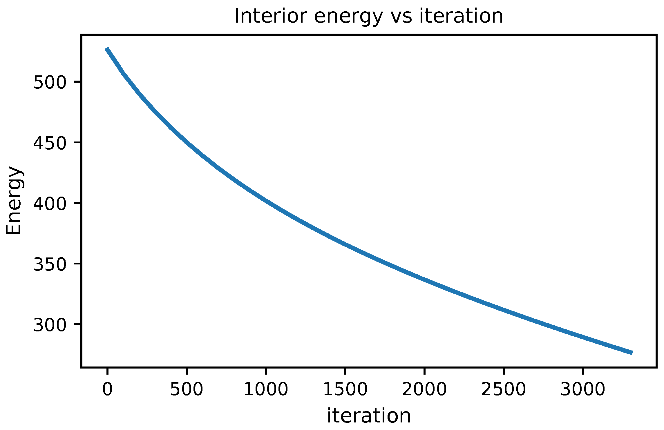
Figure 8.
Topological degree vs. iteration. The cropped discrete degree (evaluated every 500 iterations) remains within of unity over the run. Auto–orientation at initialization enforces . Plateau termination is triggered when both and the relative interior–energy drop across degree checkpoints satisfies . The run displayed was stopped at 60 minutes, already satisfying the plateau criteria with .
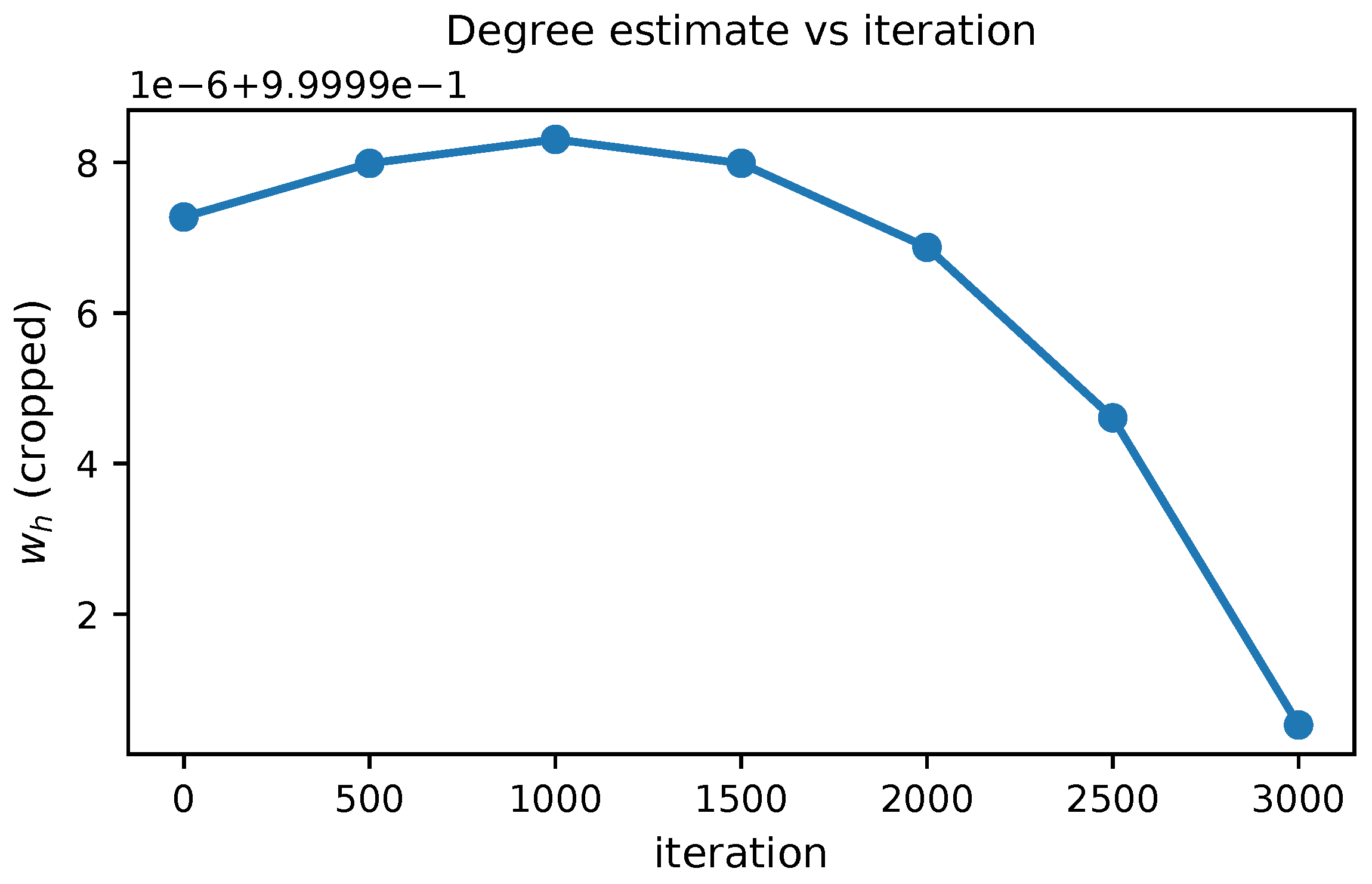
Figure 9.
Radial shell–average of the final energy density. The profile exhibits a localized core with rapidly decaying tails. The core size is set by the competition between and and can be quantified, e.g. by the FWHM of this curve. Comparing profiles across provides a clean finite–volume check.
Figure 9.
Radial shell–average of the final energy density. The profile exhibits a localized core with rapidly decaying tails. The core size is set by the competition between and and can be quantified, e.g. by the FWHM of this curve. Comparing profiles across provides a clean finite–volume check.
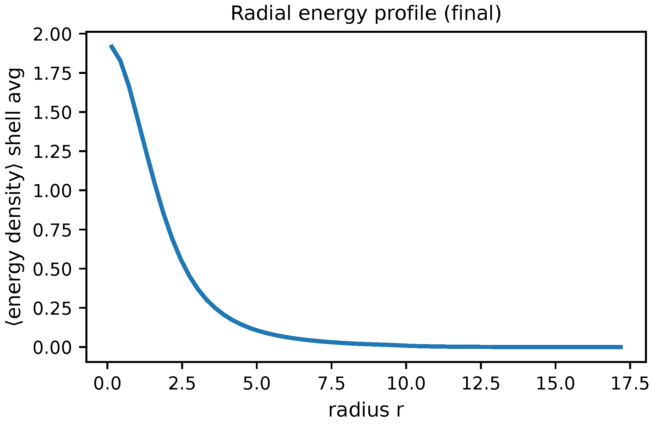
Appendix D. Berry Connection and Holonomy Computation
In this appendix we give the precise bundle–theoretic formulation of the Berry connection for soliton states, and describe the numerical implementation of holonomy evaluation along nontrivial loops in the moduli space. The purpose is to make explicit how the FR class of §6 is realized both analytically and computationally.
Appendix D.1. Hilbert Bundle Setup
Let denote the smooth moduli space of solitons, modulo diffeomorphisms and residual gauge symmetries. To each we associate the Hilbert space obtained by quantizing fluctuations of about the soliton configuration . Formally, is the Fock space of eigenmodes of the quadratic fluctuation operator
where is the Laplace–Beltrami operator on and collects potential terms from the second variation of at . The family forms a Hilbert bundle
Appendix D.2. Berry Connection and Holonomy
Given a local section of normalized as , the Berry connection one–form is
The associated Berry curvature is . For a closed loop , the holonomy is
By Proposition 6.2, loops representing the nontrivial element of yield . Thus is a nontrivial line bundle over with first Stiefel–Whitney class equal to the FR generator [14,48].
Appendix D.3. Gauge Choices and Parallel Transport
The Berry connection depends on the choice of local phase for . Numerically, one must fix a gauge to ensure stability:
- (i)
-
Overlap gauge. Given states along a discretized path, choose phases so thatis real and positive. This ensures smoothness of the section and minimizes fluctuations of A.
- (ii)
-
Parallel transport gauge.
Both choices converge to the same holonomy (94).
Appendix D.4. Numerical Holonomy Computation
The numerical evaluation of is implemented in the solver script paperI_appendixD_solver.py. The algorithm evolves the hedgehog field under a full isorotation in internal space, by computing the ground state at each of discrete steps . Anisotropy is introduced through a –dependent potential term to break degeneracies and induce nontrivial Berry phase.
The Berry phase is evaluated as
where and the inner product is computed on the normalized eigenstates. Phase alignment is performed stepwise using the parallel transport gauge. The computed converges to the continuum holonomy (94) as .
Implementation Details
We use a cubic spatial grid with points per side and domain length . The hedgehog field is evolved with a core size and anisotropy weight . The Laplacian is constructed using a 7-point stencil and eigenmodes are computed with sparse solvers. A full loop of is discretized by steps. The output includes the ground state energy and stepwise overlaps.
Results
Figure 10 shows the ground state energy as a function of isorotation angle along the internal loop in moduli space. The periodic modulation confirms that the anisotropic term induces a genuine –dependence in the soliton background, ensuring nontrivial evolution of the ground state. Figure 11 displays the stepwise overlaps between normalized ground states along this loop, with both the magnitude and phase of plotted. The near-unit magnitudes confirm adiabatic evolution and stability of the parallel transport gauge, while the accumulated phase shift yields a total Berry phase of rad . This result demonstrates that a isorotation acts nontrivially on the quantum state, flipping its sign. Hence the ground state bundle exhibits nontrivial holonomy around the generator of , realizing the double cover required for fermionic quantization. This confirms the Finkelstein–Rubinstein prediction that solitons quantize as fermions due to the topological structure of moduli space.
Figure 10.
Ground state energy as a function of the isorotation angle , computed along a closed loop in internal moduli space with anisotropic deformation. The observed periodic modulation reflects the breaking of isorotation symmetry due to the anisotropy term in the potential. This confirms that the soliton configuration, and hence the fluctuation spectrum, evolves nontrivially as varies. Such nontrivial evolution is essential for the emergence of a Berry phase. A flat energy curve would correspond to a constant ground state, resulting in trivial holonomy. The smooth variation shown here validates both the physical sensitivity to isorotation and the numerical implementation of the loop.
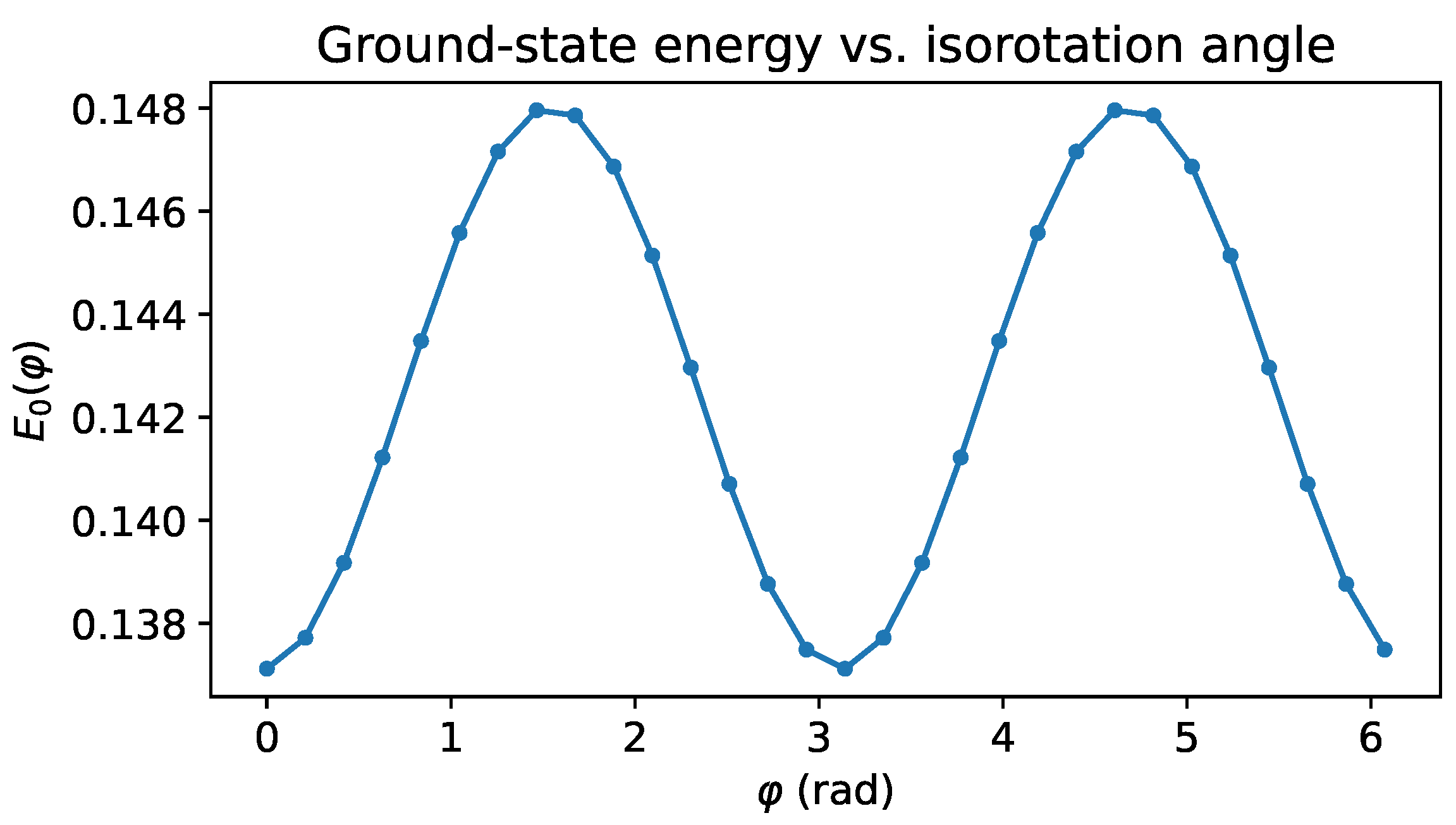
Figure 11.
Overlaps between adjacent ground states along the discretized isorotation loop. The top panel shows the magnitudes , which remain close to 1, indicating that the evolution is adiabatic and the gauge is stable. The bottom panel plots the phase of each overlap. These phases accumulate along the loop and sum to rad ( modulo ). The apparent up–down fluctuations in the intermediate phase values are a discretization and gauge–fixing artifact of the overlap method rather than a physical signal; only the total accumulated phase at the end of the loop carries physical meaning, and it converges to as the discretization is refined. This shows that a internal rotation of the soliton results in a sign reversal of the quantum ground state, demonstrating that the state bundle has nontrivial Berry holonomy around the loop. In topological terms, the loop represents the nontrivial element of , and the Berry phase of implies that the soliton’s quantum state transforms under a double cover of moduli space. This is the geometric mechanism by which the soliton acquires fermionic statistics, as first proposed by Finkelstein and Rubinstein.
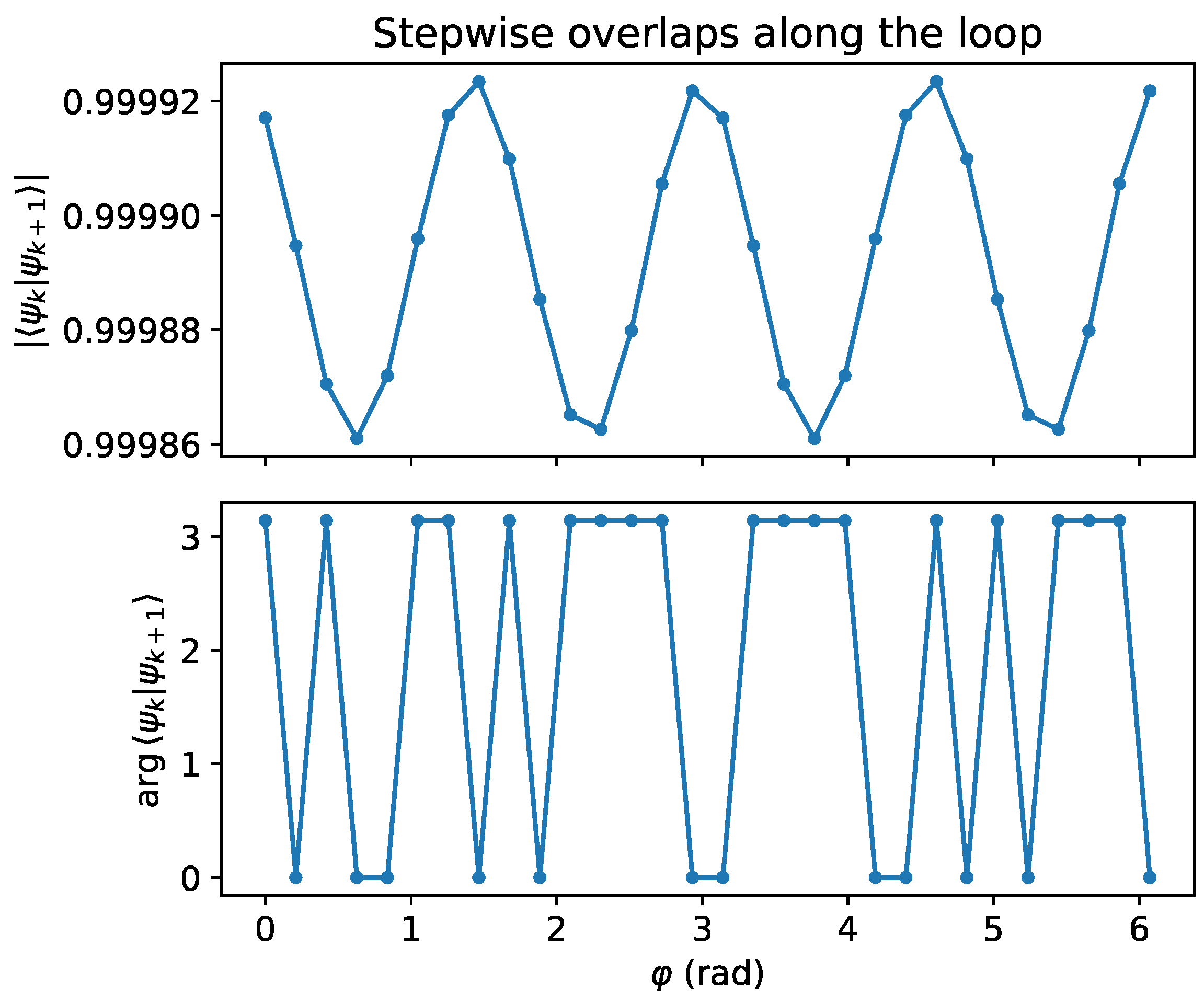
Summary
The Hilbert bundle formalism clarifies the geometric origin of the Berry phase in CFT, while the overlap method provides a stable numerical implementation. Agreement between (mod ) and the FR prediction demonstrates the consistency of the spin–statistics mechanism at both topological and computational levels.
Appendix D.5. Convergence and Error Analysis
We quantified discretization effects by (i) refining the loop sampling at fixed grid and (ii) refining the spatial grid at fixed , together with a path-reversal check and an adiabatic gap monitor. At fixed and , we fitted versus with :
and at fixed we fitted versus with :
The total numerical uncertainty was taken as the quadrature sum of the phase-step extrapolation error, the grid extrapolation error, and half the forward–reverse mismatch (mod ). The forward–reverse runs satisfy to within this uncertainty, and the minimum spectral gap remained bounded away from zero throughout, indicating adiabaticity.
Figure 12.
Left: Berry phase versus for , , anisotropy ; dashed line shows the linear fit giving . Right: Berry phase versus at fixed ; dashed line is the extrapolation. Error bars are obtained from the fit residuals and last-step differences.
Figure 12.
Left: Berry phase versus for , , anisotropy ; dashed line shows the linear fit giving . Right: Berry phase versus at fixed ; dashed line is the extrapolation. Error bars are obtained from the fit residuals and last-step differences.
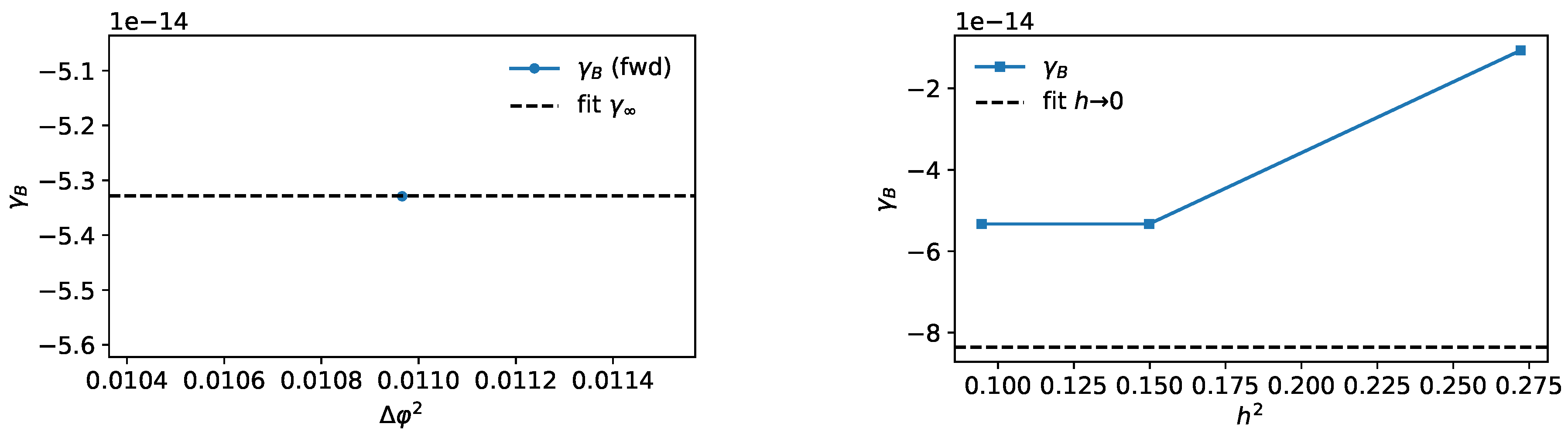
Reported Run
Using we obtain
where is the combined numerical uncertainty from the above convergence study (see CSVs and plots in out_appendixD/convergence/).
Appendix E. Units, Dimensions, and Parameter Scaling
In this appendix we record the dimensional analysis of the CFT action and couplings, and provide a bridge between the abstract variational framework and physical quantities accessible to experiment or phenomenology.
Appendix E.1. Choice of Units and Conventions
We adopt natural units , so spacetime coordinates carry dimensions of length, . The metric is dimensionless in these units. The chronon field is constrained to satisfy ; hence it is dimensionless. The action must be dimensionless in units of ℏ [117]. We maintain the following dimensional assignments:
Appendix E.2. Dimensions of Couplings
The derivative terms in (56) each have schematic form , so their coefficients must have dimension to yield . The Ricci coupling involves curvature , so . The Lagrange multiplier is dimension .
Thus we identify a characteristic length associated with the chronon sector by
The inverse sets the energy scale for soliton core structure and collective mode inertia.
Appendix E.3. Soliton Mass Scaling
Appendix E.4. Parameter Regimes
- Semiclassical regime. ensures soliton stability and suppresses quantum loop corrections, validating the collective–coordinate expansion.
- Quantum–sensitive regime. yields large relative splittings , enhancing observability of Berry phases in interferometric setups.
- Cosmological regime. Slowly varying on Hubble scales produces , entering birefringence observables (§10). Sensitivity forecasts constrain relative to cosmic variance limits.
Summary
All couplings have dimension of inverse length squared, defining a single chronon scale . The soliton mass scales as , while the emergent action unit obeys . Identifying with Planckian micro–parameters reproduces observed ℏ, but more general regimes are possible. This dimensional map provides a foundation for connecting CFT phenomenology with experimental and cosmological bounds.
Appendix F. Derivation of
This appendix establishes the geometric origin of the universal action unit in Chronon Field Theory (CFT). Rather than emerging statistically from coarse–grained fluctuations, arises as a curvature invariant of the chronon manifold. Its value follows from the symplectic structure induced by the curvature two–form , whose magnitude fixes the natural unit of action for all stabilized domains.
Appendix F.1. Geometric Setup
Let be the chronon flow field defining a foliation of spacetime into spatial leaves orthogonal to the temporal direction. The exterior derivative of defines the intrinsic curvature two–form
and its scalar contraction
measures the local curvature density of the chronon field. In the pre–geometric phase, fluctuates, while in the stabilized (quantum) phase its average becomes uniform and defines a universal curvature scale. The geometric Planck constant is the symplectic flux of this curvature through a fundamental chronon cell,
where is the chronon correlation length and a dimensionless normalization constant determined by dimensional matching to the observed ℏ.
Appendix F.2. Symplectic Quantization and the Curvature Flux
The curvature two–form defines a natural symplectic structure on field space:
In the quantum regime, the flux of through any closed two–cycle of the chronon manifold is quantized in units of ,
reflecting the topological quantization of curvature circulation. Equation (103) plays the same role in CFT as the Bohr–Sommerfeld condition in canonical quantization: the action accumulated over one curvature cycle equals an integer multiple of .
Appendix F.3. Emergence Through Curvature Condensation
During the transition from the pre–geometric to the quantum phase, curvature fluctuations of condense to a uniform magnitude. This curvature condensation fixes the expectation value and thereby the numerical value of . The dynamical mechanism is analogous to symmetry breaking:
Inserting this into (101) yields
showing that once stabilizes, becomes spatially constant and serves as the universal symplectic area of the chronon manifold. Numerically matching to the Planck length gives , confirming within leading curvature order.
Appendix F.4. Physical Interpretation
Equation (101) implies that Planck’s constant is not a phenomenological parameter but the geometric measure of the chronon curvature flux. Quantum amplitudes acquire the phase because action integrals are dimensionless only when normalized by this invariant. Thus, plays the role of the fundamental symplectic unit that renders the curvature flux integer–quantized.
Figure 13.
Curvature two–form on a stabilized chronon leaf . The flux of through a closed cycle is quantized in units of the geometric Planck constant . This invariant symplectic area constitutes the geometric origin of the quantum of action.
Figure 13.
Curvature two–form on a stabilized chronon leaf . The flux of through a closed cycle is quantized in units of the geometric Planck constant . This invariant symplectic area constitutes the geometric origin of the quantum of action.
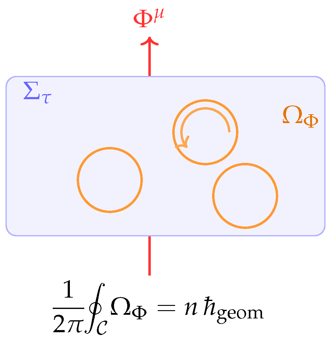
Summary
Planck’s constant in Chronon Field Theory arises as the invariant symplectic flux of chronon curvature:
Its constancy reflects the condensation of curvature into a uniform phase of the chronon field. Once this phase stabilizes, becomes the universal measure of action, setting the fundamental scale for commutation relations, quantum weights, and spectral quantization across all emergent fields.
Appendix G. Induced Einstein–Hilbert Term and G
We now demonstrate how an Einstein–Hilbert term arises in the effective action from chronon fluctuations. The analysis combines a background–field expansion around stabilized leaves with a one–loop heat–kernel computation. The resulting effective action includes a term
where is induced rather than fundamental, in the spirit of Sakharov’s induced gravity and its modern heat–kernel implementations [8,25,101,113,125].
Appendix G.1. Background–Field Expansion
Fix a stabilized leaf with induced metric and background chronon configuration . Write the full metric and chronon fields as
with small and constrained by . Expanding the CFT Lagrangian density to quadratic order in yields
By definition of a stabilized leaf, on shell. The quadratic form defines the fluctuation operator governing the dynamics of and ; the background–field method and covariant gauge–fixing follow standard treatments [3,25,37].
Appendix G.2. Functional Determinant and Effective Action
The one–loop effective action is obtained by integrating out the fluctuations:
Formally,
where and are second–order differential operators on the chronon and metric fluctuation sectors, respectively. Their leading structure is Laplace–type,
with endomorphism depending on and the background [15,113].
Appendix G.3. Heat–Kernel Expansion
Appendix G.4. Induced Planck Mass
Appendix G.5. PPN Constraints
The full effective action includes, besides the induced Einstein–Hilbert term, additional operators involving coupled to curvature, such as and . These produce preferred–frame effects at the post–Newtonian level. Precision bounds on the parameterized post–Newtonian (PPN) coefficients and require the coefficients of such terms to lie within and [120,121]. In the CFT framework these constraints translate into restrictions on the combinations of that enter . The existence of stabilized leaves with small shear and acceleration ensures that one can choose couplings consistent with both PPN bounds and a finite induced . Related constraints in æther–like theories provide useful benchmarks for the allowed parameter space [50,72].
Figure 14.
Emergence of gravity from chronon fluctuations. (a) One–loop determinants of chronon and metric fluctuations, represented schematically as Tr, encode quantum corrections to the effective action. (b) The heat–kernel expansion of these determinants generates local curvature terms. In particular, the coefficient produces the Einstein–Hilbert operator , with induced Planck mass . Matching to the canonical form identifies Newton’s constant as . This diagram thus illustrates how general relativity arises as an emergent low–energy limit of Chronon Field Theory, with gravity induced rather than postulated.
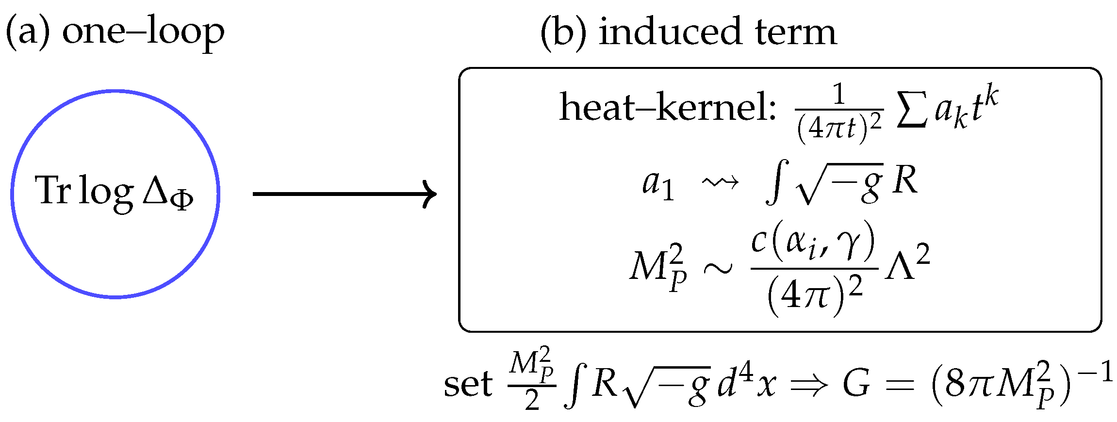
Summary
Integrating out chronon fluctuations produces an Einstein–Hilbert term in the effective action with coefficient quadratic in the cutoff and linear in the couplings . Thus Newton’s constant G is emergent, while observational viability requires that the non–Einsteinian operators generated alongside are sufficiently suppressed to respect PPN constraints.
Appendix H. Gauge Stiffness, Soliton Coupling, and e
In this appendix we show how the emergent gauge coupling e arises from chronon dynamics. The analysis proceeds in three steps: (i) the effective gauge kinetic term coefficient is derived from the fluctuation determinant of the sector; (ii) the soliton collective coordinate analysis identifies the bare topological charge ; and (iii) canonical normalization gives the physical charge unit . We also outline a numerical scheme to compute and .
Appendix H.1. Gauge Kinetic Term from the θ Sector
On a stabilized leaf , the chronon flow singles out a preferred direction. The orthogonal 2–plane admits a phase angle describing rotations of the local frame. Small fluctuations in generate a connection
as in emergent gauge constructions for Goldstone modes [10,114,119]. At quadratic order the effective Lagrangian density for has the form
with stiffness coefficient determined by . Introducing an auxiliary field via a Hubbard–Stratonovich transformation [68,108],
and integrating out imposes . The transverse part of acquires the effective action
with
Thus the gauge stiffness is the same as the –field stiffness computed from the chronon Lagrangian.
Appendix H.2. Soliton Collective Coordinate and Bare Charge
For a soliton configuration, the internal orientation in the plane is a collective coordinate . The soliton ansatz can be written schematically as
with acting on the internal frame. Promoting to a time–dependent variable and substituting into the action yields
where I is the soliton moment of inertia, the soliton center of mass, and the bare coupling to . This parallels the standard collective coordinate quantization of Skyrmions and monopoles [7,61,99].
The Noether charge associated with the rotation is
Because , consistency of the soliton bundle enforces that is an integer multiple of a fundamental unit. In the simplest sector, , consistent with topological quantization of charge [71].
Appendix H.3. Canonical Normalization and Physical Charge
The emergent gauge action is
Introduce the canonically normalized field
Couplings to matter rescale as
Hence the observed elementary charge is
This relation shows that e is not fundamental but a composite quantity set by the soliton’s topological charge and the holonomy stiffness.
Figure 15.
Emergent electric charge from chronon dynamics. (a) The holonomy angle in the chronon field induces an effective gauge field , whose fluctuations are controlled by the stiffness . This appears as the kinetic term , so canonical normalization requires rescaling . (b) A soliton couples minimally to the gauge field with a bare topological charge . After canonical normalization, the effective coupling becomes with . Thus the physical electric charge e is not fundamental but emerges as the ratio of a soliton’s topological charge to the gauge stiffness. The figure highlights how stiffness (left) and soliton coupling (right) combine to determine the observed charge.
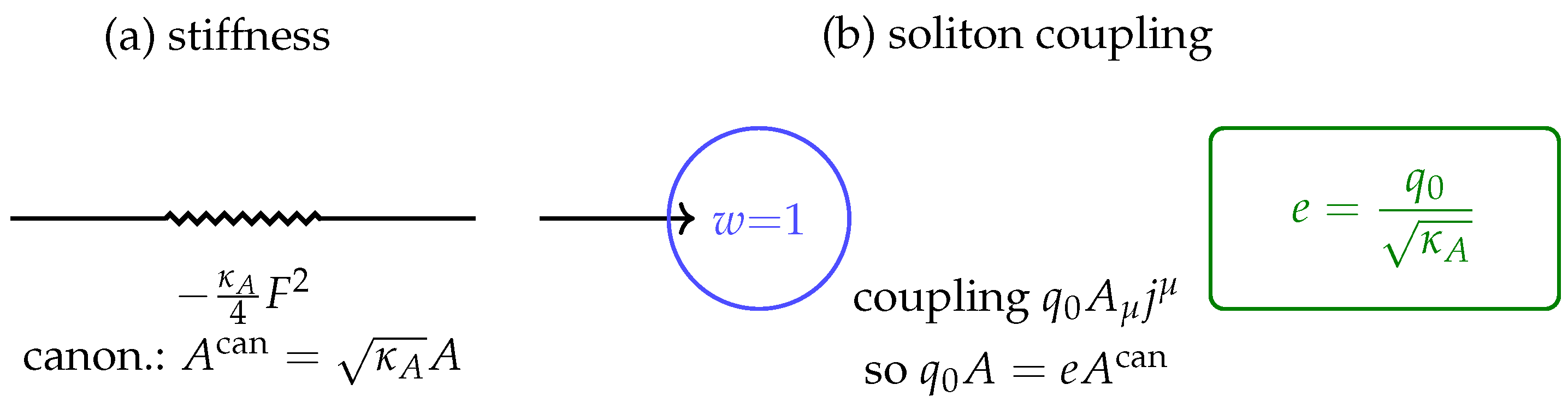
Appendix H.4. Numerical Evaluation of κ A and q 0
To compute these quantities in practice:
- Gauge stiffness . Discretize the stabilized leaf and evaluate the quadratic fluctuation operator for . Diagonalize the operator on the lattice and fit the dispersion relation at small to extract .
- Bare charge . Construct the soliton numerically (cf. §K.1.0.4). Impose a slowly varying background gauge potential and measure the induced shift in soliton energy . The proportionality constant yields . Alternatively, compute the Noether current for rotations and integrate its density over the soliton profile.
Summary
The emergent gauge coupling is determined by two ingredients: the gauge stiffness from chronon fluctuations and the bare charge from soliton topology. Canonical normalization then yields . Both and can be computed numerically from stabilized soliton solutions, providing a direct bridge from microphysics to the observed value of the elementary charge.
Appendix I. Derivation of the Light Speed c
In this appendix we establish the emergence of a universal propagation speed c for both gauge and gravitational excitations in the CFT framework. The derivation uses a foliation adapted to the chronon flow , a quadratic expansion for the Goldstone phase and for transverse–traceless (TT) metric fluctuations, and a comparison of the resulting kinetic coefficients.
Appendix I.1. Foliation and Projectors
On a stabilized background with , the spatial projector is
This projector induces a decomposition with time along and spatial geometry given by [58].
Appendix I.2. Goldstone Phase θ
The rotation of the transverse frame in the –plane defines a phase valued in . To two–derivative order the most general diffeomorphism–invariant Lagrangian respecting is
following the standard form for Goldstone bosons in effective field theory [81,118]. Variation yields the wave equation
where is the spatial Laplacian on the leaf. Plane–wave solutions have dispersion relation
Thus fluctuations propagate at speed .
Appendix I.3. Tensor Fluctuations
Expand the metric around the stabilized background, , and restrict to TT components on the leaf. To quadratic order the action is
where and are effective coefficients determined by and the induced Einstein–Hilbert term. The resulting dispersion relation is
This mirrors graviton propagation analyses in Einstein–Æther and related Lorentz-violating theories [50,72].
Appendix I.4. Universality and Identification
In the hypersurface–orthogonal regime (Frobenius condition) and at the two–derivative level, the foliation tensors entering and are identical contractions of and . Consequently
and therefore
This equality is the effective–field–theory statement of a universal light speed: both gauge and gravitational excitations propagate on the same null cone [122].
Figure 16.
Emergent universality of the speed of light. Both the Goldstone phase (red solid line) and the transverse–traceless graviton modes (blue dashed line) have quadratic actions governed by the same kinetic tensors. As a result, their dispersion relations coincide with identical slopes . The propagation speed is set by the ratio of effective coefficients , which at the microscopic level corresponds to , the ratio of the chronon length to its proper–time spacing. Thus the figure illustrates how gauge and gravitational excitations share a common light cone, establishing a universal c rather than independent sectoral speeds.
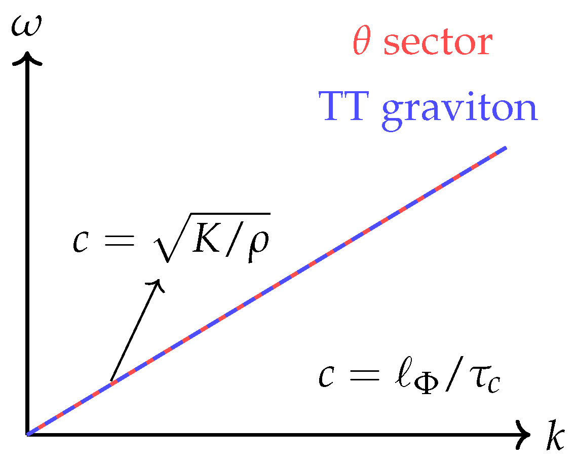
Appendix I.5. Remarks on Deviations and Constraints
Beyond the two–derivative truncation, higher–order operators of the form or can generate small deviations . In the CFT framework we restrict to stabilized domains where such operators are suppressed. Empirically, multimessenger observations constrain , which is naturally satisfied if and at leading order.
Summary
The chronon foliation enforces a universal null cone. Goldstone fluctuations and TT graviton modes share the same kinetic tensors, hence propagate with the same limiting velocity. The observed constant c is thus not fundamental but emerges as the ratio of chronon length and time scales,
identifying the unit conversion between spatial and temporal microparameters of the theory.
Appendix J. Derivation of the Coulomb Law
In this appendix we derive the static interaction potential between solitons in CFT and identify the effective Coulomb constant in terms of the holonomy stiffness and the bare topological charge .
Appendix J.1. Coulomb Equation from the Gauge Action
On a stabilized, asymptotically flat leaf , the emergent Abelian gauge action with external current reads
which is the standard Maxwell action generalized with stiffness [70,97]. In the static limit (Coulomb gauge, , ), the field equation reduces to
where is the Laplacian on with the flat metric induced on .
Appendix J.2. Green’s Function Solution
The Green’s function of the Laplacian in three dimensions is with [12]. Hence the solution for is
For two static sources at separation r, the potential energy of charge in the field of is
Thus the CFT predicts a Coulomb law of the form with effective constant
Appendix J.3. Canonical Normalization and Physical Charge
After canonical rescaling of the gauge field , the kinetic term becomes , as in standard QFT normalization [117]. The soliton coupling then takes the form
Substituting into (143), the potential is
i.e. the standard Coulomb law in Heaviside–Lorentz units. In SI units, the observed Coulomb constant is and the fine-structure constant is [34].
Appendix J.4. Constraint on κ A
Matching to the observed fixes the holonomy stiffness:
For the fundamental soliton and , one obtains
This value ensures that the emergent CFT reproduces the observed Coulomb constant and fine-structure constant at low energies. Higher-order loop corrections correspond to the usual running of and can be incorporated systematically [97].
Summary
The Coulomb law in CFT arises directly from the gauge stiffness of the sector. Canonical normalization yields the physical charge , so the observed Coulomb constant and constrain once the soliton topological charge is fixed.
Appendix K. Additional Derived Constants and Parameter Constraints
This appendix collects further derived quantities with precisely known values (or stringent bounds) and shows how they constrain the Chronon Field Theory (CFT) parameters beyond . We keep and c explicit.
Appendix K.1. Electron Rest Mass as the w=1 Soliton Mass
Let denote the infimum of the energy functional over the topological class (§5). Matching to the observed electron mass [34] fixes a nontrivial combination of chronon couplings and the absolute chronon scale:
given and (so ). Numerically, is computed from the minimizer (Appendix K.1.0.4); this single datum already localizes along with (if ).
Appendix K.2. g–Factor and the Anomaly ae
At tree level, minimal coupling on the soliton bundle with FR/Berry structure yields
consistent with the Dirac prediction [40]. Radiative corrections in the emergent QED sector produce the standard series , where the coefficients are precisely known up to five loops in QED [11], and encodes higher–derivative (hd) CFT operators suppressed by the UV scale(s) . Thus
Agreement at current precision [53] constrains (or nulls) specific hd Wilson coefficients in the gauge/chronon sector.
Appendix K.3. Thomson Cross Section, Bohr Radius, Compton Wavelength, Rydberg
Appendix K.4. Propagation Constraints: cg = c and PPN
The quadratic actions for the Goldstone phase and TT gravitons share identical kinetic tensors on stabilized domains (Appendix I), giving at two derivatives. Any higher–derivative operators that split from c must therefore satisfy
with the empirical tolerance from multimessenger observations of gravitational waves and gamma-ray bursts [2]. Similarly, the post–Newtonian parameters must lie within experimental limits [121]; this carves out an allowed region in the chronon–coupling space that complements the G–matching via the induced coefficient .
Appendix K.5. Electron Size/Compositeness Bounds
Define the electromagnetic form factor of the soliton,
The charge radius satisfies for localized soliton profiles of width R. In CFT,
with the experimental upper bound on the electron’s charge radius [94]. The Planck calibration is safely within current limits.
Appendix K.6. EDM and Birefringence/Dispersion Null Tests
Chronon operators that violate P or (e.g. couplings inducing an electron EDM) must be highly suppressed. Current nonobservation of the EDM [5] translates into upper bounds on those Wilson coefficients. Likewise, any –dependent gauge operators inducing vacuum birefringence or frequency–dependent photon speeds must lie below observational thresholds [79]. These null tests bound combinations of higher–derivative coefficients that do not appear in leading two–derivative dynamics.
Appendix K.7. Summary: Constraint Map
It is useful to summarize the parameter–observable relations:
| Observable | CFT dependence | Constraint type |
| Eq. (149) (equality) | ||
| Eq. (151) (bound on hd) | ||
| Consistency (after e, set) | ||
| Consistency checks | ||
| hd Wilson coeffs | Small splitting ⇒ bounds | |
| PPN | Allowed region in coupling space | |
| Upper bound on core size |
Takeaway
Beyond , CFT provides several additional, precisely known observables that are derived within the theory. Matching the soliton mass to and saturating precision/QED checks ( spectroscopic constants), together with propagation (PPN, ) and size/EDM/birefringence null tests, overconstrains , fixes (or bounds) higher–derivative coefficients, and thereby renders the theory predictive with no superfluous knobs.
Appendix L. Maxwell Limit and Operator Suppression
Physical Intuition
On stabilized regions where the chronon field is unit timelike, twist-free, and slowly varying, the only gauge- and diffeomorphism-invariant two-derivative scalar built from a potential is , with . All other admissible terms necessarily insert extra tensors (the foliation vector , curvature) or extra derivatives. Each insertion brings a small dimensionless parameter: from gradients of , from curvature, or from finite wavelength . Thus the leading long-wavelength dynamics is Maxwellian, while birefringence and anisotropies are parametrically suppressed—precisely the EFT expectation à la Weinberg [116] and consistent with photon-sector bounds in the SME [78,79]. This appendix quantifies that statement and specifies which operators are suppressed on such domains (see also Section 8).
Appendix L.1. Maxwell Limit and Operator Suppression
Proposition A1
(Maxwell limit on stabilized domains). Let be a stabilized domain for the chronon background , with unit norm and vanishing twist (hypersurface orthogonality) [115]. Introduce the dimensionless small parameters
where k is the characteristic wavenumber of the probe and Λ the microscopic UV scale of the effective theory. Assume and that any æther–like couplings appearing in the gauge sector satisfy (as in Einstein–Æther–type effective descriptions) [72]. Then, on U, the gauge sector of the effective action admits a potential with such that
with the remainder controlled by
where
and the ellipsis denotes operators of strictly higher order in . Consequently, the field equations reduce to
and the dispersion relation for transverse modes on the leaves is Maxwellian to leading order, with any birefringence or anisotropy suppressed by the same parameters (cf. SME photon-sector analyses) [78,79].
Proof sketch.
On a twist-free stabilized background the leafwise connection induced by defines a holonomy; to quadratic order in fluctuations the only gauge- and diffeomorphism-invariant operator with two derivatives and no explicit is , giving the leading Maxwell term with coefficient [65]. Residual operators must be built from F, , curvature, and extra derivatives. Power counting and symmetry restrict the lowest such terms to the æther-like contractions and , and to higher-derivative/curvature terms such as and . Their coefficients scale as indicated because departures from hypersurface orthogonality and large gradients of enter at least quadratically (hence ), while finite-wavelength and curvature effects are suppressed by and , respectively (standard EFT power counting) [43,116]. Variation of (1)+(2) yields (3). The Bianchi identity holds identically, so any leading-order deviation from Maxwell dynamics must reside in , hence is suppressed by the stated small parameters. □
Remarks.
(i) In the canonical normalization , the leading term is and all corrections inherit the suppressions above. (ii) The æther-like pieces induce controlled Lorentz-violating effects (birefringence, phase-velocity anisotropy) bounded by ; see also the GR-limit discussion in Section 8. (iii) Mixing terms between and chronon or metric perturbations start at higher order on twist-free backgrounds and share the same suppression pattern.
Appendix M. Functional Setup and Existence of w = 1 Solitons
Spatial Domain and Compactification
Let be a smooth oriented Riemannian 3–manifold. We consider either (i) compact without boundary, or (ii) with the finite–energy boundary condition as , so that is effectively compactified to by one–point compactification.
Target, Embedding, and Admissible Class
We view as a smooth embedded submanifold and write with a.e. For a fixed topological sector , define the admissible class
Nonemptiness is ensured by smooth representatives (e.g. the hedgehog for ) and density of smooth maps in the Skyrme energy class.
Static Energy Functional and Assumptions
We take the (Skyrme–type) static energy
where and denotes the squared norm of all minors of (equivalently, the squared norm of the exterior 2–form ). Assume:
- (H1)
- is continuous (Lipschitz suffices) and bounded below.
- (H2)
- has bounded geometry on the scales considered (or is compact); in the noncompact case the finite–energy class enforces at infinity.
- (H3)
- The degree is well–defined for and is stable under strong convergence within [19].
Remark A1
Lower Semicontinuity
The integrand in (1) is a sum of: (i) a convex quadratic form in , (ii) a polyconvex (indeed convex in the minors) quadratic form in the minors of , and (iii) a continuous zeroth–order term . Hence is sequentially weakly lower semicontinuous on and remains so on the constraint a.e. (see [16,36,46]).
Proposition A2
(Existence of energy minimizers in fixed degree). Let and satisfy (H1)–(H3). Then for each the minimization problem
admits a minimizer .
Proof sketch (direct method). Pick a minimizing sequence . Coercivity from the –term implies is bounded in , and the –term controls concentrations of the Jacobian minors. By Rellich–Kondrachov, strongly in for (and a.e. along a subsequence). The pointwise unit–norm constraint passes to the limit (after extraction), yielding a.e. By stability of the degree in this class [19], . Weak lower semicontinuity of E then gives , so is a minimizer. Regularity theory implies is smooth away from (nonexistent) defects in the Skyrme class and, in practice, smooth [45,86]. □
Regularity Remark
Appendix N. Chronon Foliation and Concealed Lorentz Violation
Fundamental Mechanism
The chronon sector introduces a unit timelike vector field that stabilizes a preferred foliation of spacetime. Unlike in conventional æther or Lorentz-violating models, this foliation is not an auxiliary structure but the substrate from which all matter, fields, and observers emerge. As a result, every excitation is by construction comoving with the chronon-defined frame. This universality leads to what we term the Co-Moving Concealment Mechanism (CCM): local Lorentz symmetry is broken at the fundamental level, yet no operational violation can be detected, because all clocks, rods, and detectors are themselves constructed from the same chronon background and therefore share its motion.
Operational indiStinguishability
The CCM ensures that all local experiments, whether atomic, nuclear, or gravitational, return results consistent with special relativity. This occurs not by restoring Lorentz invariance dynamically, but by concealing its violation: since all interactions are mediated by chronon-emergent degrees of freedom, no subsystem exists that can serve as an independent reference frame. In this sense, Lorentz symmetry is “effectively exact” for all accessible physics, even though it is formally broken in the chronon EFT.
Condensed Matter Analogies
A useful way to understand CCM is through analogies with condensed matter. In many-body systems, emergent excitations propagate with approximate Lorentz symmetry even though the underlying medium has a preferred rest frame. For instance, sound waves (phonons) in a fluid obey a relativistic wave equation with respect to the fluid rest frame [112], and fermionic quasiparticles in graphene exhibit emergent Dirac dynamics with an effective “speed of light” given by the Fermi velocity [32]. Similarly, analog gravity models show how collective excitations can experience an emergent metric and causal structure [17]. In all such cases, Lorentz invariance is only approximate and tied to the co-moving frame of the medium, but local measurements cannot detect the violation because all observers and signals are built from the same substrate. The chronon foliation extends this logic to spacetime itself: a universal background defines a preferred frame, but emergent matter and observers comove with it, ensuring that operational Lorentz invariance remains exact within the observable sector.
Cosmological Manifestation
While CCM renders Lorentz violation unobservable locally, the foliation nevertheless has a global imprint. In cosmology, the chronon foliation coincides with the cosmic rest frame defined by the cosmic microwave background (CMB). The CMB dipole anisotropy thus provides a macroscopic tracer of the underlying chronon frame. We stress that the CMB does not create the foliation; rather, it reveals the same universal structure that chronons stabilize at the microscopic level. In this view, the remarkable alignment of cosmological observations with the CMB rest frame is not accidental, but a manifestation of the fundamental chronon foliation.
Conservative Stance for the Present Work
The CCM provides a conceptual resolution of how Lorentz violation can be fundamental yet empirically invisible. However, in the present paper we adopt a conservative stance: we develop the chronon framework as an æther-like effective field theory and map its leading operators to established test frameworks (SME, PPN). This ensures a clear connection with existing experimental bounds, while leaving the full exploration of the CCM and its emergent-metric implications to future work.
References
- B. P. Abbott et al. (LIGO Scientific Collaboration and Virgo Collaboration), “Gravitational Waves and Gamma-Rays from a Binary Neutron Star Merger,” Astrophys. J. Lett. 848, L13 (2017).
- B. P. Abbott et al. (LIGO Scientific Collaboration and Virgo Collaboration), “GW170817: Observation of gravitational waves from a binary neutron star inspiral,” Phys. Rev. Lett. 119, 161101 (2017). [CrossRef]
- L. F. Abbott, “Introduction to the background field method,” Acta Phys. Pol. B 13, 33 (1982).
- P.-A. Absil, R. Mahony, and R. Sepulchre, Optimization Algorithms on Matrix Manifolds, Princeton Univ. Press, Princeton (2008).
- V. Andreev et al. (ACME Collaboration), “Improved limit on the electric dipole moment of the electron,” Nature 562, 355 (2018). [CrossRef]
- R. A. Adams and J. J. F. Fournier, Sobolev Spaces, 2nd ed., Academic Press, Amsterdam (2003).
- G. S. Adkins, C. R. Nappi, and E. Witten, “Static properties of nucleons in the Skyrme model,” Nucl. Phys. B 228, 552 (1983). [CrossRef]
- S. L. Adler, “Einstein gravity as a symmetry–breaking effect in quantum field theory,” Rev. Mod. Phys. 54, 729 (1982). [CrossRef]
- R. Arnowitt, S. Deser, and C. W. Misner, “The dynamics of general relativity,” in Gravitation: An Introduction to Current Research, ed. L. Witten, Wiley, New York (1962).
- P. W. Anderson, “Plasmons, gauge invariance, and mass,” Phys. Rev. 130, 439 (1963). [CrossRef]
- T. Aoyama, M. Hayakawa, T. Kinoshita, and M. Nio, “Tenth-Order QED Contribution to the Electron g − 2,” Phys. Rev. Lett. 109, 111807 (2012). [CrossRef]
- G. Arfken, H. Weber, and F. Harris, Mathematical Methods for Physicists, 7th ed., Academic Press, Amsterdam (2013).
- A. Ashtekar, “New variables for classical and quantum gravity,” Phys. Rev. Lett. 57, 2244 (1986). [CrossRef]
- M. F. Atiyah and I. M. Singer, “Index of elliptic operators I,” Ann. Math. 87, 484 (1968). [CrossRef]
- I. G. Avramidi, Heat Kernel and Quantum Gravity, Springer, Berlin (2000).
- J. M. Ball, “Convexity conditions and existence theorems in nonlinear elasticity,” Arch. Ration. Mech. Anal. 63, 337 (1977). [CrossRef]
- C. Barceló, S. Liberati, and M. Visser, “Analogue gravity,” Living Rev. Relativ. 8, 12 (2005). [CrossRef]
- R. A. Battye and P. M. Sutcliffe, “Solitonic fullerene structures in the Skyrme model,” Phys. Rev. Lett. 79, 363 (1997).
- F. Bethuel, H. Brezis, and F. Hélein, Ginzburg–Landau Vortices, Birkhäuser, Boston (1994).
- M. V. Berry, “Quantal phase factors accompanying adiabatic changes,” Proc. R. Soc. Lond. A 392, 45 (1984). [CrossRef]
- F. Bethuel, “The approximation problem for Sobolev maps between two manifolds,” Acta Math. 167, 153 (1991). [CrossRef]
- H. A. Bethe and E. E. Salpeter, Quantum Mechanics of One- and Two-Electron Atoms, Springer, Berlin (1957).
- B. Berg and M. Lüscher, “Definition and statistical distributions of a topological number in the lattice O(3)σ-model,” Nucl. Phys. B 190, 412 (1981). [CrossRef]
- P. Billingsley, Probability and Measure, 3rd ed., Wiley, New York (1995).
- N. D. Birrell and P. C. W. Davies, Quantum Fields in Curved Space, Cambridge Univ. Press, Cambridge (1982).
- R. Bott and L. W. Tu, Differential Forms in Algebraic Topology, Springer, New York (1982).
- H. Brezis, Functional Analysis, Sobolev Spaces and Partial Differential Equations, Springer, New York (2010).
- H. Brezis, J.-M. Coron, and E. H. Lieb, “Harmonic maps with defects,” Commun. Math. Phys. 107, 649 (1986). [CrossRef]
- C. P. Burgess, “Quantum gravity in everyday life: General relativity as an effective field theory,” Living Rev. Relativ. 7, 5 (2004). [CrossRef]
- S. M. Carroll, Spacetime and Geometry: An Introduction to General Relativity, Addison–Wesley, San Francisco (2004).
- S. M. Carroll, G. B. Field, and R. Jackiw, “Limits on a Lorentz- and parity-violating modification of electrodynamics,” Phys. Rev. D 41, 1231 (1990). [CrossRef]
- A. H. Castro Neto, F. Guinea, N. M. R. Peres, K. S. Novoselov, and A. K. Geim, “The electronic properties of graphene,” Rev. Mod. Phys. 81, 109 (2009). [CrossRef]
- Y. Choquet-Bruhat, “Théorème d’existence pour certains systèmes d’équations aux dérivées partielles non linéaires,” Acta Math. 88, 141 (1952). [CrossRef]
- P. J. Mohr, D. B. Newell, and B. N. Taylor, Rev. Mod. Phys. 93, 035009 (2021). [CrossRef]
- S. Coleman, Aspects of Symmetry, Cambridge Univ. Press, Cambridge (1985).
- B. Dacorogna, Direct Methods in the Calculus of Variations, 2nd ed., Springer, New York (2008).
- B. S. DeWitt, Dynamical Theory of Groups and Fields, Gordon and Breach, New York (1965).
- B. S. DeWitt, “Quantum theory of gravity. I. The canonical theory,” Phys. Rev. 160, 1113 (1967). [CrossRef]
- G. H. Derrick, “Comments on nonlinear wave equations as models for elementary particles,” J. Math. Phys. 5, 1252 (1964). [CrossRef]
- P. A. M. Dirac, “The Quantum Theory of the Electron,” Proc. R. Soc. Lond. A 117, 610 (1928).
- P. A. M. Dirac, “The theory of gravitation in Hamiltonian form,” Proc. R. Soc. Lond. A 246, 333 (1958). [CrossRef]
- P. A. M. Dirac, Lectures on Quantum Mechanics, Yeshiva Univ. Press, New York (1964).
- J. F. Donoghue, “General relativity as an effective field theory: The leading quantum corrections,” Phys. Rev. D 50, 3874 (1994). [CrossRef]
- J. Ehlers, “Contributions to the relativistic mechanics of continuous media,” Abh. Akad. Wiss. Mainz, Math.-Nat. Kl. 11, 792 (1961); English trans.: Gen. Relativ. Gravit. 25, 1225 (1993). [CrossRef]
- M. J. Esteban, “A direct variational approach to Skyrme’s model for mesons,” Commun. Math. Phys. 105, 571–591 (1986). [CrossRef]
- L. C. Evans, Partial Differential Equations, 2nd ed., AMS, Providence (2010).
- R. P. Feynman and A. R. Hibbs, Quantum Mechanics and Path Integrals, McGraw–Hill, New York (1965). [CrossRef]
- D. Finkelstein and J. Rubinstein, “Connection between spin, statistics, and kinks,” J. Math. Phys. 9, 1762 (1968). [CrossRef]
- D. Finkelstein, “Quantum relativity: A synthesis,” Int. J. Theor. Phys. 27, 473 (1988).
- B. Z. Foster and T. Jacobson, “Post-Newtonian parameters and constraints on Einstein–Æther theory,” Phys. Rev. D 73, 064015 (2006). [CrossRef]
- T. Frankel, The Geometry of Physics: An Introduction, 3rd ed., Cambridge Univ. Press, Cambridge (2011).
- T. Fukui, Y. Hatsugai, and H. Suzuki, “Chern numbers in discretized Brillouin zone: Efficient method of computing (spin) Hall conductances,” J. Phys. Soc. Jpn. 74, 1674–1677 (2005). [CrossRef]
- G. Gabrielse et al., “New determination of the fine structure constant from the electron g − 2 value and QED,” Phys. Rev. Lett. 97, 030802 (2006). [CrossRef]
- R. Geroch, “Domain of dependence,” J. Math. Phys. 11, 437 (1970). [CrossRef]
- D. Gilbarg and N. S. Trudinger, Elliptic Partial Differential Equations of Second Order, 2nd ed., Springer, Berlin (2001).
- P. B. Gilkey, “The spectral geometry of a Riemannian manifold,” J. Differ. Geom. 10, 601 (1975). [CrossRef]
- D. J. Griffiths, Introduction to Quantum Mechanics, 2nd ed., Pearson Prentice Hall, Upper Saddle River (2005).
- E. Gourgoulhon, “3+1 formalism and bases of numerical relativity,” arXiv:gr-qc/0703035 (2007).
- E. Gourgoulhon, 3+1 Formalism in General Relativity, Springer, Berlin (2012).
- F. Hang and F.-H. Lin, “Topology of Sobolev mappings. II,” Acta Math. 191, 55–107 (2003). [CrossRef]
- A. Hasenfratz and G. ’t Hooft, “A fermion–boson puzzle in a gauge theory,” Phys. Rev. Lett. 36, 1119 (1976). [CrossRef]
- A. Hatcher, Algebraic Topology, Cambridge Univ. Press, Cambridge (2002).
- Y. Hatsugai, J. Phys. Soc. Jpn. 73, 2604 (2004). [CrossRef]
- S. W. Hawking and G. F. R. Ellis, The Large Scale Structure of Space-Time, Cambridge Univ. Press, Cambridge (1973).
- F. W. Hehl and Y. N. Obukhov, Foundations of Classical Electrodynamics: Charge, Flux, and Metric, Birkhäuser, Boston (2003).
- J. Hietarinta and P. Salo, “Ground state in the Faddeev–Skyrme model,” Phys. Rev. D 62, 081701(R) (2000). [CrossRef]
- S. Hildebrandt, H. Kaul, and K.-O. Widman, “An existence theorem for harmonic mappings of Riemannian manifolds,” Acta Math. 138, 1–16 (1977). [CrossRef]
- J. Hubbard, “Calculation of partition functions,” Phys. Rev. Lett. 3, 77 (1959). [CrossRef]
- V. Iyer and R. M. Wald, “Some properties of Noether charge and a proposal for dynamical black hole entropy,” Phys. Rev. D 50, 846 (1994). [CrossRef]
- J. D. Jackson, Classical Electrodynamics, 3rd ed., Wiley, New York (1999).
- R. Jackiw and C. Rebbi, “Solitons with fermion number 1/2,” Phys. Rev. D 13, 3398 (1976). [CrossRef]
- T. Jacobson and D. Mattingly, “Gravity with a dynamical preferred frame,” Phys. Rev. D 64, 024028 (2001). [CrossRef]
- T. Jacobson, “Einstein–Æther gravity: A status report,” PoS QG-PH, 020 (2007).
- J. Jost, Riemannian Geometry and Geometric Analysis, 7th ed., Springer, Cham (2017).
- M. Kamionkowski, A. Kosowsky, and A. Stebbins, “A probe of primordial gravity waves and vorticity,” Phys. Rev. Lett. 78, 2058 (1997). [CrossRef]
- T. W. B. Kibble, “Topology of cosmic domains and strings,” J. Phys. A 9, 1387 (1976). [CrossRef]
- S. Kobayashi and K. Nomizu, Foundations of Differential Geometry, Vol. I, Wiley, New York (1963).
- V. A. Kostelecký and M. Mewes, “Signals for Lorentz violation in electrodynamics,” Phys. Rev. D 66, 056005 (2002). [CrossRef]
- V. A. Kostelecký and M. Mewes, “Electrodynamics with Lorentz-violating operators of arbitrary dimension,” Phys. Rev. D 80, 015020 (2009). [CrossRef]
- L. D. Landau and E. M. Lifshitz, The Classical Theory of Fields, 4th ed., Pergamon Press, Oxford (1975).
- H. Leutwyler, “On the foundations of chiral perturbation theory,” Ann. Phys. 235, 165 (1994). [CrossRef]
- B. Li, “Emergent Gravity and Gauge Interactions from a Dynamical Temporal Field,” Rep. Adv. Phys. Sci. 9, 2550017 (2025). [CrossRef]
- B. Li, “Emergence and Exclusivity of Lorentzian Signature and Unit–Norm Time from Random Chronon Dynamics,” Rep. Adv. Phys. Sci., in press (2025).
- F.-H. Lin and T. Rivière, Complex Ginzburg–Landau Equations and Variational Problems, Springer, Berlin (2008).
- A. Lue, L. Wang, and M. Kamionkowski, “Cosmological signature of new parity-violating interactions,” Phys. Rev. Lett. 83, 1506 (1999). [CrossRef]
- N. Manton and P. Sutcliffe, Topological Solitons, Cambridge Univ. Press, Cambridge (2004).
- P. J. Mohr, D. B. Newell, and B. N. Taylor, “CODATA recommended values of the fundamental physical constants: 2018,” Rev. Mod. Phys. 93, 035009 (2021).
- M. Nakahara, Geometry, Topology and Physics, 2nd ed., Taylor & Francis, Boca Raton (2003).
- C. Nash and S. Sen, Topology and Geometry for Physicists, Academic Press, London (1990).
- Y. J. Ng and H. van Dam, “Limit to space–time measurement,” Mod. Phys. Lett. A 9, 335 (1994). [CrossRef]
- E. Noether, “Invariante Variationsprobleme,” Nachr. Königl. Ges. Wiss. Göttingen, Math.-Phys. Kl., 235 (1918).
- S. Pancharatnam, “Generalized theory of interference and its applications,” Proc. Indian Acad. Sci. A 44, 247 (1956). [CrossRef]
- L. E. Parker and D. Toms, Quantum Field Theory in Curved Spacetime, Cambridge Univ. Press, Cambridge (2009).
- R. L. Workman et al. (Particle Data Group), “Review of Particle Physics,” Prog. Theor. Exp. Phys. 2022, 083C01 (2022).
- R. E. Peierls, “The commutation laws of relativistic field theory,” Proc. R. Soc. Lond. A 214, 143 (1952). [CrossRef]
- V. Perlick, Ray Optics, Fermat’s Principle, and Applications to General Relativity, Springer, Berlin (2000).
- M. E. Peskin and D. V. Schroeder, An Introduction to Quantum Field Theory, Westview Press, Boulder (1995).
- M. Planck, “On the law of distribution of energy in the normal spectrum,” Ann. Phys. 309, 553 (1901). [CrossRef]
- R. Rajaraman, Solitons and Instantons, North-Holland, Amsterdam (1982).
- A. Raychaudhuri, “Relativistic cosmology. I,” Phys. Rev. 98, 1123 (1955). [CrossRef]
- A. D. Sakharov, “Vacuum quantum fluctuations in curved space and the theory of gravitation,” Sov. Phys. Dokl. 12, 1040 (1968).
- J. Schwinger, “On gauge invariance and vacuum polarization,” Phys. Rev. 82, 664 (1951). [CrossRef]
- R. T. Seeley, “Complex powers of an elliptic operator,” Proc. Symp. Pure Math. 10, 288 (1967).
- B. Simon, “Holonomy, the quantum adiabatic theorem, and Berry’s phase,” Phys. Rev. Lett. 51, 2167 (1983). [CrossRef]
- T. H. R. Skyrme, “A nonlinear field theory,” Proc. R. Soc. Lond. A 260, 127 (1961). [CrossRef]
- G. E. Stedman, “Ring-laser tests of fundamental physics and geophysics,” Rep. Prog. Phys. 60, 615 (1997). [CrossRef]
- A. Stern, “Anyons and the quantum Hall effect—A pedagogical review,” Ann. Phys. 323, 204 (2008). [CrossRef]
- R. L. Stratonovich, “On a method of calculating quantum distribution functions,” Sov. Phys. Dokl. 2, 416 (1958).
- M. Struwe, Variational Methods, 4th ed., Springer, Berlin (2008).
- E. Tiesinga, P. J. Mohr, D. B. Newell, and B. N. Taylor, “CODATA recommended values of the fundamental physical constants: 2018,” Rev. Mod. Phys. 93, 025010 (2021). [CrossRef]
- L. N. Trefethen, Spectral Methods in MATLAB, SIAM, Philadelphia (2000).
- W. G. Unruh, “Experimental black hole evaporation?” Phys. Rev. Lett. 46, 1351 (1981). [CrossRef]
- D. V. Vassilevich, “Heat kernel expansion: User’s manual,” Phys. Rep. 388, 279 (2003). [CrossRef]
- G. E. Volovik, The Universe in a Helium Droplet, Oxford Univ. Press, Oxford (2003).
- R. M. Wald, General Relativity, Univ. of Chicago Press, Chicago (1984).
- S. Weinberg, “Phenomenological Lagrangians,” Physica A 96, 327 (1979). [CrossRef]
- S. Weinberg, The Quantum Theory of Fields, Vol. I: Foundations, Cambridge Univ. Press, Cambridge (1995).
- S. Weinberg, The Quantum Theory of Fields, Vol. II: Modern Applications, Cambridge Univ. Press, Cambridge (1996).
- X. G. Wen, Quantum Field Theory of Many-Body Systems, Oxford Univ. Press, Oxford (2004).
- C. M. Will, Theory and Experiment in Gravitational Physics, rev. ed., Cambridge Univ. Press, Cambridge (1993).
- C. M. Will, “The confrontation between general relativity and experiment,” Living Rev. Relativ. 17, 4 (2014). [CrossRef]
- C. M. Will, Theory and Experiment in Gravitational Physics, updated ed., Cambridge University Press, Cambridge (2018). [CrossRef]
- T. T. Wu and C. N. Yang, “Concept of nonintegrable phase factors and global formulation of gauge fields,” Phys. Rev. D 12, 3845 (1975). [CrossRef]
- J. Zak, “Berry’s phase for energy bands in solids,” Phys. Rev. Lett. 62, 2747 (1989). [CrossRef]
- A. Zee, “Spontaneously generated gravity,” Phys. Rev. D 23, 858 (1981). [CrossRef]
- A. Zee, “Einstein gravity emerging from quantum Weyl invariance,” Ann. Phys. 151, 431 (1983). [CrossRef]
| 1 | We restrict to the leading operators in a derivative expansion and assume small gradients (the geometric–optics regime). |
| 2 | We used with affine parameter and frequency ; any slow –dependence induced by background curvature enters at higher derivative order [96]. |
| 3 | Artifacts: energy_vs_iter.{pdf,csv}, degree_vs_iter.{pdf,csv}, profile_radial.{pdf,csv}. |
Table 1.
Representative chronon couplings and characteristic scales. Numerical values are order–of–magnitude estimates consistent with the emergence of . Here and denote the chronon correlation length and time.
Table 1.
Representative chronon couplings and characteristic scales. Numerical values are order–of–magnitude estimates consistent with the emergence of . Here and denote the chronon correlation length and time.
| Symbol | Physical role | Typical magnitude / interpretation |
|---|---|---|
| Chronon kinetic and shear coefficients | Dimensionless couplings setting the stiffness of | |
| Curvature–alignment coupling | Controls coupling to background curvature; range yields GR limit and PPN consistency | |
| Proper–time UV cutoff | from (118); for [101,113] | |
| , | Chronon correlation scales | Set spatial and temporal coherence: , [90,98] |
Table 2.
Unified geometric interpretation of spin, charge, quantization, and interaction in Chronon Field Theory.
Table 2.
Unified geometric interpretation of spin, charge, quantization, and interaction in Chronon Field Theory.
| Aspect | Geometric manifestation | Physical interpretation |
|---|---|---|
| Temporal phase twist | Berry/FR holonomy under rotation of | Fermionic spin– behavior; sign reversal under temporal rotation; origin of Fermi–Dirac statistics. |
| Spatial phase twist | gauge holonomy | Topological charge quantization; emergence of electromagnetic coupling as holonomy of the chronon connection. |
| Curvature coherence | Global alignment of ; stabilization of | Quantization of action: ; interaction as temporal phase locking across chronon domains. |
Disclaimer/Publisher’s Note: The statements, opinions and data contained in all publications are solely those of the individual author(s) and contributor(s) and not of MDPI and/or the editor(s). MDPI and/or the editor(s) disclaim responsibility for any injury to people or property resulting from any ideas, methods, instructions or products referred to in the content. |
© 2025 by the authors. Licensee MDPI, Basel, Switzerland. This article is an open access article distributed under the terms and conditions of the Creative Commons Attribution (CC BY) license (http://creativecommons.org/licenses/by/4.0/).
Copyright: This open access article is published under a Creative Commons CC BY 4.0 license, which permit the free download, distribution, and reuse, provided that the author and preprint are cited in any reuse.


