
Submitted:
25 September 2025
Posted:
07 October 2025
You are already at the latest version
Abstract
The primary aim of this paper is to explore and comprehend the abstraction underlying the mechanisms of the universe. Based on our current understanding, which is deeply intertwined with mathematics, it is estimated that our universe is approximately 14 billion years old. By adopting specific assumptions and axioms, one can construct a model universe and trace its subsequent evolution; however, it is evident that such constructed universes are not the one in which we exist. Rather, these abstract universes are developed through the application of advanced mathematical frameworks to demonstrate that, given appropriate assumptions, it is indeed possible to formulate a coherent representation of a universe. Nevertheless, experimental verification remains indispensable for validating any such theoretical endeavors. Furthermore, when considering multiverse theories, this paper contends that even in the presence of infinitely many possible universes, the probability of their actual existence is not necessarily substantial.The central theme of this work revolves around two fundamental questions: What is truly meant when we invoke the concept of a “universe” and its subsequent evolution? And what underlying principles enable a universe to be structured with such precision—down to its fundamental constants and intricate details—that it can sustain itself and evolve over billions of years? To address these questions, the paper examines two abstract universes: (A) the Fractal Universe, denoted as U3, and (B) the Abstract ζ-Function Universe, denoted as U4. The structural and cosmological evolution of these universes is described, followed by a comparative analysis and a discussion of the philosophical consequences of constructing such abstract mathematical models.
Keywords:
universe
; cosmology
; fractal geometry
; mathematics
; philosophy
1. Introduction
Every scientific inquiry begins with a fundamental premise, and every theoretical framework necessitates a foundational starting point. In the context of the universe as we currently understand it, there exists a discernible beginning. However, this perception remains largely speculative, derived from observational evidence and theoretical extrapolation. It is plausible that an alternative perspective, or a more sophisticated mathematical language, could provide a deeper understanding of the universe’s fundamental nature. Mathematics, coupled with technological advancements, has proven to be an indispensable tool in constructing our comprehension of existence.
Current cosmological observations suggest that the universe is approximately 14 billion years old [8]. Naturally, this curiosity compels us to ask fundamental questions such as: Does the universe have a beginning, or has it always existed? Does the universe contain matter and energy, or is it entirely empty? Is the universe homogeneous and isotropic, or is it anisotropic and non-uniform? Is the universe static, expanding, or contracting? Each combination of these parameters results in drastically different cosmological scenarios. Consider a hypothetical universe that possesses the following features: it has a beginning, is infinite in spatial extent, is non-homogeneous, is anisotropic, and is dynamic but not expanding.
How would such a universe behave? Many of these theoretical configurations may contradict physical laws or empirical observations. Furthermore, if we were to slightly alter any fundamental cosmic parameter, how drastically would it affect the resulting structure, history, and geometry of the universe? Could a minute shift in initial conditions redefine the very fabric of space-time? Why does the universe exist in its current form? A compelling insight is provided by Stephen Hawking in Black Holes and Baby Universes and Other Essays, where he discusses the prerequisites for the emergence of intelligent life:
“According to one version of the principle, there is a very large number of different, separate universes with different values of the physical parameters and different initial conditions. Most of the universes will not provide the right conditions for the development of the complicated structures needed for intelligent life. …Will it be possible for intelligent life to develop and to ask the question, `Why is the universe as we observe it?’ The answer, of course, is that if it were otherwise there would not be anyone to ask the question.” [2]
This perspective aligns with the Anthropic Principle, which posits that the observed values of the universe’s parameters must be compatible with the existence of observers—otherwise, such observations could never be made. Thus, the essential question emerges: Is the configuration of our universe uniquely determined, or could alternative configurations also give rise to intelligent life and structured reality? Understanding the arrangement of cosmic parameters with mathematical precision is vital to developing coherent and predictive cosmological models. As this paper introduces abstract mathematical universes, it is important to understand why mathematical abstraction is so crucial. To quote Bertrand Russell: “Mathematics, rightly viewed, possesses not only truth, but supreme beauty, cold and austere …capable of a stern perfection such as only the greatest art can show” [9].
“Mathematics, rightly viewed, possesses not only truth, but supreme beauty, cold and austere, like that of sculpture, without appeal to any part of our weaker nature, without the gorgeous trappings of painting or music, yet sublimely pure, and capable of a stern perfection such as only the greatest art can show. The true spirit of delight, the exaltation, the sense of being more than Man, which is the touchstone of the highest excellence, is to be found in mathematics as surely as in poetry.”[9]
Such mathematical frameworks are employed in this paper to analyze abstract universes [10,11]. Mathematical functions provide an elegant means of describing the evolution and complexity of these universes. The hypothetical universes discussed here are based on certain mathematical functions; essentially, these universes are constructed from such abstract functions, and their evolution helps determine the conditions that prevail at specific points in time [1]. To construct a hypothetical universe, it is necessary to first establish a set of axioms and assumptions, which serve as the fundamental building blocks of the framework [7]. The axioms are defined as follows:—
1. There exists an abstract space , which constitutes the abstract universe. Within this framework, we define parametric universes , where . These parametric universes are generated and evolve according to parametric functions.
2. Parametric functions are expressed as .
3. There exists a transition operation defined by:
This transition drives the evolution and complexity corresponding to each respective universe.
From these axioms, we introduce the following assumptions:
1. Parametric universes emerge from the parametric space like bubbles arising from an ocean. (The underlying mechanism of this emergence is not our concern; we assume it as a given.) 2. Transitions occur at a well-defined time , which we will analyze with respect to the parameters under consideration.
With these axioms and assumptions, we can construct parametric universes and study their evolution and complexity. In the paper, two such universes are discussed. One example is the Fractal Universe, denoted as , which is relatively simple and directly aligned with fractal geometry as studied in mathematics [3]. The other example involves a more unusual structure, where the function is identified with the so-called -function. In this case, the resulting evolution gives rise to infinitely many possible scenarios, depending on the equations and assumptions considered.
2. Building Hypothetical Universes
2.1. Fractal Parametric Universe ()
The Parametric Universe emerged from the parametric axioms. A fundamental aspect of this universe is the presence of a parametric function , which encapsulates the essential configurations of the parametric universe. Notably, exhibits fractal behavior and possesses a distinct origin, with its evolution governed by two distinct scenarios: (a) a case involving a singular function, referred to as the unitary parametric function, and (b) a case involving multiple functions, referred to as the multitary parametric function. These cases give rise to unique spatial and temporal configurational behaviors throughout the universe.
The parametric function is formally defined as:
where (Functional A) and (Functional B) are the initial parametric function that emerged at the inception of the parametric universe from the abstract space. Among these, Functional is given by:
with the parameters and defined as:
This function represents the fractal dimension of space-time, which varies with direction, thereby resulting in an anisotropic universe. Here, and are parameters, where denotes the polar angle and denotes the azimuthal angle. The functional , representing the fractal dimension, varies between 2 and 3 based on the defined expression. This directional dependence reflects anisotropies in the spatial structure of the universe. The density profile associated with this fractal dimension is given by:
where r denotes the radial distance. This relation reveals that the density scaling behavior is directly controlled by the directional fractal dimension . For instance, at , where , the density scales as , indicating a mild divergence near the origin. In contrast, at , where , the density becomes uniform ().
This anisotropic scaling behavior implies that matter distribution is directionally dependent, leading to denser clustering in directions where . Consequently, such a universe exhibits observable anisotropies in cosmic structures—potentially manifesting as elongated galaxies, filaments, or walls aligned with specific angular directions [7].The exponent varies within the range , meaning that density either decreases with radius or remains constant depending on direction. In regions where , the density declines more slowly with increasing radius, resulting in higher concentration of matter near the origin. However, this effect remains moderate and directionally bounded. The fractal nature of this universe, governed by the parametric function , allows for self-similar structures across scales [3,4,5], indicating a hierarchical pattern of structure formation. Unlike smooth manifolds, this fractal space-time has a non-integer dimension between 2 and 3, suggesting a geometry that is rougher than a 2D surface but not fully three-dimensional. The variation of introduces directional dependence into the spatial configuration, thus breaking isotropy and leading to anisotropic space. In such a universe, spatial properties and matter distribution are functions of direction. Directions with lower D not only exhibit slower decay in density but also feature more pronounced clustering near the origin—possibly corresponding to the early formation of high-density structures such as protogalaxies. Conversely, directions with exhibit uniform density, leading to more diffuse matter distribution.
Figure 1.
Evolution of Universe –Initial Phase (the Python code used to generate the graphs is available on GitHub)
Figure 1.
Evolution of Universe –Initial Phase (the Python code used to generate the graphs is available on GitHub)
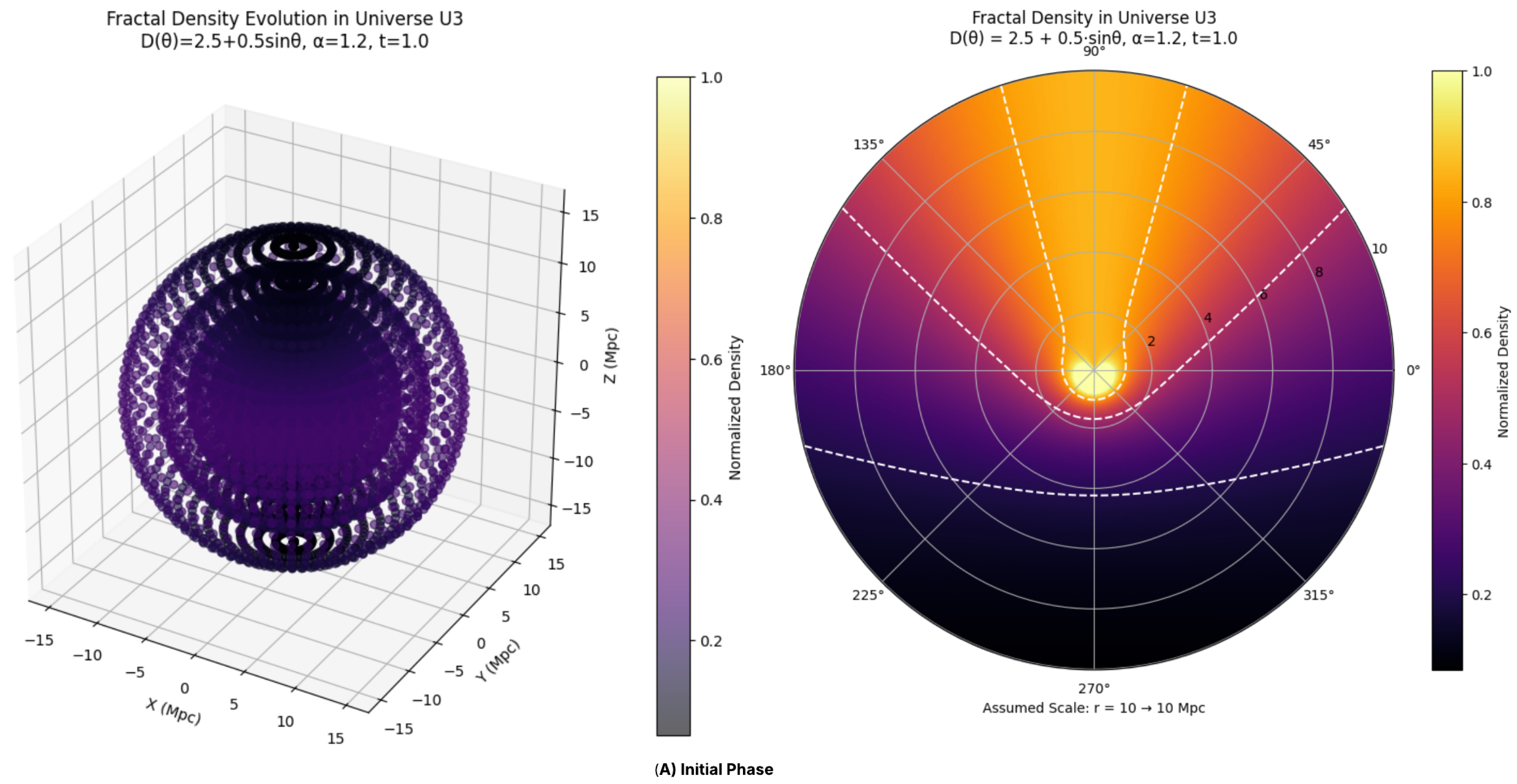
For an observer O within this universe, these anisotropies would be apparent in the observed cosmic web—denser galaxy clusters or filaments would appear aligned with specific directions, while other regions would seem more sparsely populated. The range of between 2 and 3 reinforces the fractal, self-similar character of cosmic structures, implying that galaxy clusters and other large-scale features form hierarchically and repeat similar patterns across different scales. The universe in this framework is assumed to begin at , corresponding to in the spatial density profile. When , the density diverges at , leading to a direction-dependent singularity. Such an anisotropic singularity implies that structure formation could proceed more rapidly along those directions, reinforcing the idea that early structure formation is more prominent where the fractal dimension is lower, whereas in directions with , the singular behavior is absent or greatly suppressed. Altogether, this framework presents a compelling picture: a universe that did not simply begin, but rather unfolded asymmetrically, giving rise to its intricate cosmic web through fractal rules. The direction-dependent fractal dimension not only governs the distribution of matter but also defines the very character of space itself. From this perspective, the cosmos emerges as a system rich in structure, scale, and directional identity—offering not just a single narrative, but a tapestry of intertwined evolutionary paths embedded within an anisotropic, dynamically evolving geometry. Having explored Functional A, we now turn to Functional B, which plays a critical role in governing the influence of the fractal dimension on the universe’s structural and temporal evolution.
Here, represents the fractional order of the dynamical equations that govern time evolution within the parametric universe. The choice is essential to ensure the presence of a cosmological beginning (a singularity at ). For the purposes of this model, is fixed at 1.2. While it acts as a constant placeholder, its physical significance is profound—it encapsulates how physical processes unfold over time via fractional differential equations.
As discussed earlier, matter in this universe adheres to a fractal distribution, with mass scaling as . Functional B governs how such mass-energy distributions evolve by introducing fractional temporal dynamics into the field equations. For a scalar field , the evolution equation takes the form:
Here, denotes the Caputo fractional derivative, and is the fractal Laplacian adjusted for the spatially varying fractal dimension , governing spatial propagation in anisotropic space. The fractional derivative introduces non-locality in time, meaning that the evolution of the field at any moment t depends on its entire history, not merely its instantaneous state. In the case of , the Caputo derivative is defined as:
with . The kernel weights past contributions, implying that more recent times have a greater influence on current evolution. This memory effect is a hallmark of fractional dynamics, introducing complexity and feedback from earlier states of the universe [16].
Physically, the right-hand side of the evolution equation includes a potential term , which acts as a restoring force for the scalar field, and , which reflects spatial diffusion modified by the anisotropic geometry defined through . The choice has deep cosmological significance. When , the fractional derivative diverges at , amplifying the effects of initial conditions [14,17]. This behavior causes field quantities like density or itself to diverge, manifesting as a cosmological singularity—a definable starting point for the parametric universe, marked by the emergence of the parametric function .
Moreover, the non-local nature of the fractional derivative means that earlier states influence the present, introducing a kind of ’cosmological memory.’ This could explain, for example, how early-universe conditions continue to affect structure formation in a non-trivial, time-integrated manner. The evolution of deviates from standard exponential or linear behavior, potentially exhibiting pulsations, anomalous diffusion, or oscillatory modes due to this long-range temporal dependence.
A crucial implication of is that the system undergoes superdiffusion, where particles or fields spread more rapidly than under normal diffusion. This accelerates the propagation of matter and energy, leading to faster structure formation—especially in the vicinity of the origin where and . The scalar field , which could be interpreted analogously to a cosmological field such as the inflaton, exhibits a sharp singular behavior at the beginning, followed by superdiffusive dynamics as the universe evolves.
Furthermore, since the singularity at aligns with the spatial divergence at , the fractal geometry implies that the degree of divergence varies with direction. This supports the idea that early structure formation is highly anisotropic, with denser clustering in directions where the fractal dimension is lower. Such dynamics may give rise to unusual clustering patterns or early formation of dense protostructures, consistent with the behavior dictated by both Functional A and Functional B of the parametric function [24].
In summary, Functional B introduces a temporally non-local, memory-dependent mechanism that governs the dynamical evolution of fields within the parametric universe. By fixing the fractional order at , it provides a framework in which the universe originates from a well-defined beginning, evolves through superdiffusive processes, and retains a causal memory of its initial conditions. This interplay ultimately shapes the formation and distribution of cosmic structures in conjunction with the anisotropic fractal geometry prescribed by .
We now introduce the concept of a diverse parametric function, where different functionals come into play, shaping the overall evolution of the parametric universe. As illustrated in Figure, the universe undergoes three distinct phases, beginning with an initial phase governed by an early combinatorial configuration, corresponding to the moment when the parametric universe emerges from the parametric field.
In this initial setup, we consider a fractal dimension of the form , and a fractional temporal order . This configuration defines Functional A and Functional B, respectively. The fractal dimension varies between 2 and 3 as a function of the polar angle , introducing spatial anisotropy, while the fractional order governs temporal dynamics, ensuring both a cosmological beginning and non-local evolution. During this phase, the density profile is given by:
In directions where , density decreases more slowly with radius, leading to higher concentrations of matter near the origin—this anisotropic behavior results in directional clustering, with denser regions forming along specific angular directions.
Following this, the universe undergoes a first transition, marked by the emergence of new functionals— Functional C and Functional D—that significantly alter the system’s behavior. In this phase, Functional C is defined as:
Simplifying, this gives , representing a dramatic shift in the fractal dimension. Functional D, the temporal functional, remains unchanged with , thus maintaining the same non-local and singular temporal dynamics established in the initial phase.
The new density profile, still governed by:
now spans an exponent range from to . Unlike the earlier phase, where density decreased or remained constant with radius, the new profile exhibits increasing density with increasing radius across all directions. For example, at angles where , we have , while at the maximum , . This behavior signifies a complete reversal in matter distribution: instead of being densest at the origin, matter now becomes sparser near the center and accumulates more densely at larger radii.
This has profound implications for the structural evolution of the universe. The increase in fractal dimension beyond 3 indicates a spatial geometry that is even more compact and self-similar than a standard 3D manifold, potentially supporting hyper-dense clustering far exceeding what is possible in conventional cosmology [4,5]. As matter begins to migrate outward due to this density gradient, the universe develops a shell-like structure, where matter predominantly accumulates at greater radial distances, creating a sparse central region and a dense outer shell.
Furthermore, the anisotropic nature of introduces directional dependence into this shell formation [3] . In directions where is highest, the radial growth of density is steepest, resulting in non-uniform shell thickness and directional variations in the clustering intensity. Consequently, this phase of the universe may resemble a hollow-core structure, with matter density increasingly concentrated along outer regions, varying by angular direction. Despite the continued presence of a singularity due to , the nature of the singularity shifts. Because , the density as , meaning that the central singularity becomes less pronounced in terms of matter density. Instead, the focus of structural development moves outward, where the steep increase in density dominates the evolution.
Figure 2.
Second Phase

In summary, during this first transition phase, the parametric universe experiences a critical transformation. The density profile evolves from a decreasing (or constant) function of radius to an increasing power-law, with matter redistribution leading to the formation of an anisotropic, dense outer shell and a sparse inner core. This transformation preserves temporal non-locality while introducing a radically new spatial configuration governed by a high-dimensional fractal geometry.
The second transition in the evolution of the parametric universe is governed by a new set of functionals, labeled Functional E and Functional F, collectively denoted as . In this phase, the parametric function changes again, with Functional E defined by a more complex angular dependence of the fractal dimension:
This expression yields an approximate minimum of near , and a maximum around , while avoiding the singularities introduced by at . Therefore, for a practical analysis, we consider , excluding regions near the singularities.
Figure 3.
Third Phase
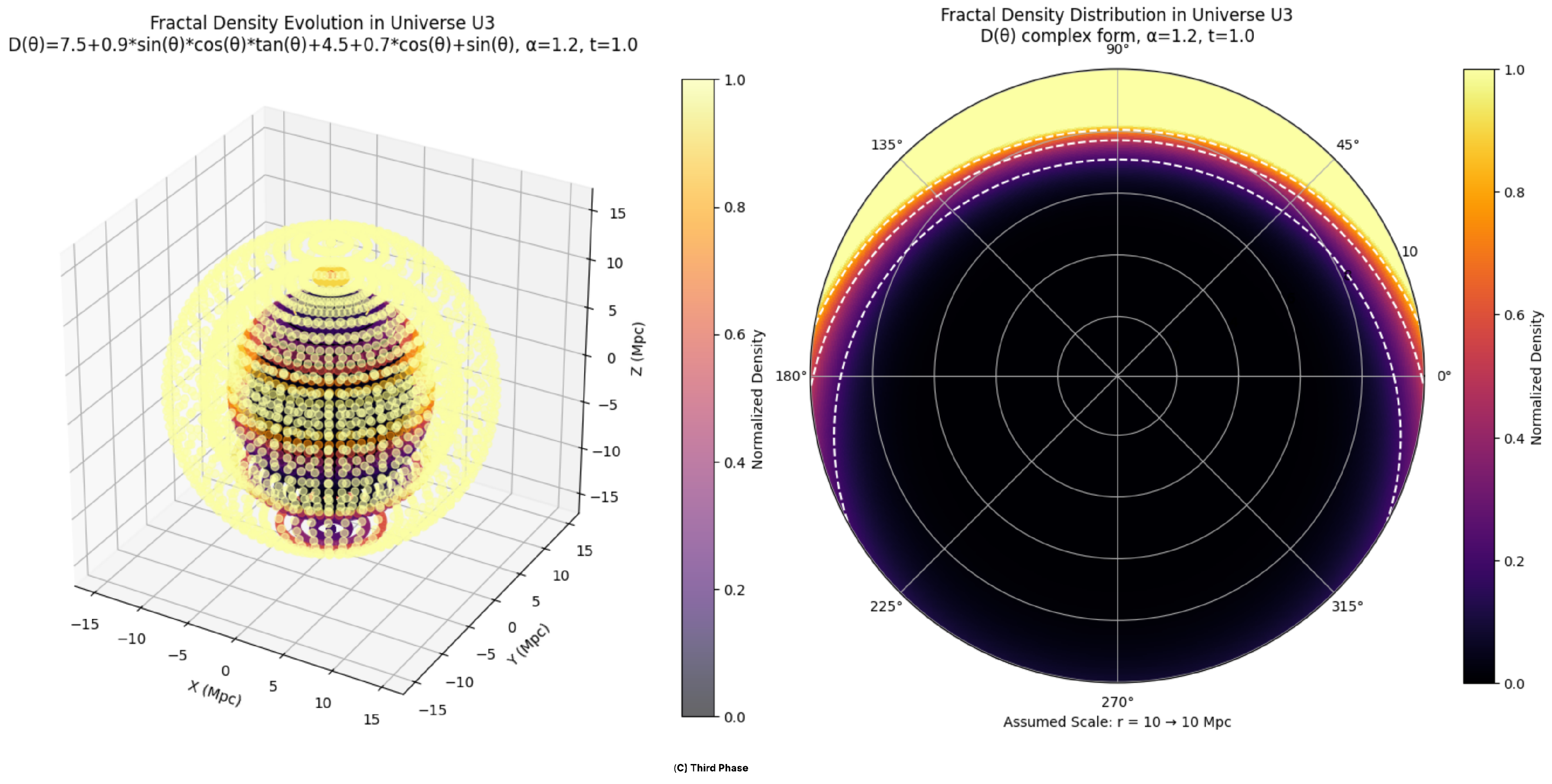
Functional F remains unchanged with , preserving the same fractional temporal dynamics established in earlier phases. This ensures the continuation of non-local evolution and a singular origin throughout all transitions [16,17].
The corresponding density profile, again governed by:
now exhibits an exponent ranging from 9.7 to 10.65. This represents an extremely steep increase in density with respect to radius—even more extreme than in the first transition [14]. This behavior underscores the intent of this phase: to explore the consequences of higher-order fractal structures in the parametric universe .
Fractal dimensions in the range of 12–13.6 vastly exceed the physical dimensionality of conventional space, implying a highly compact geometry with extreme self-similarity at multiple scales. This leads to further structural complexity and suggests the possibility of hyper-dense fractal clustering. The density increase is now so rapid that matter is pushed even farther outward, making the central regions increasingly sparse while the outer regions become hyper-dense.
Anisotropy continues to persist, as still depends on direction, causing directional variations in the steepness of density increase. However, the general trend is dominated by the sharp radial dependence, resulting in a universe with a pronounced shell-like structure. Structures form almost exclusively at the periphery, and the variation in fractal dimension causes directional differences in shell thickness, further amplifying anisotropic effects. The central singularity at remains intact due to , maintaining a singular temporal origin. However, because , the density as , meaning the singularity becomes less significant in terms of matter density but continues to dominate the temporal evolution of scalar fields such as , particularly due to memory effects inherent in fractional dynamics.
In summary, the universe evolves through three distinct structural phases:
1. Initial Phase: An anisotropic fractal universe with , leading to denser regions near the origin.
2. First Transition: A shift to , causing outward migration of matter and the formation of a dense outer shell with a sparse core.
3. Second Transition: A further increase to , resulting in an even more extreme redistribution of matter—near-total evacuation of the core and a hyper-dense peripheral shell.
Throughout all these phases, the fractional temporal order remains fixed, enforcing non-local evolution and ensuring a singular beginning. As the spatial structure evolves—from a moderately anisotropic configuration to a radially dominated and highly structured shell-like universe—the temporal singularity remains the primary driver of dynamics for scalar fields like , while the matter distribution undergoes profound restructuring.
The growth of the parametric universe is thus not characterized by conventional expansion but rather by a progressive restructuring of matter, driven by the increasing fractal dimensionality. This evolution redefines the spatial configuration, forming increasingly complex and directionally dependent structures while retaining the foundational temporal characteristics imposed by fractional dynamics.
To reconstruct the fractal universe with greater generality, we now introduce variation in both the fractal function and the fractional dynamics parameter across different evolutionary phases. This extension allows us to analyze how the combined variation in spatial dimensionality and temporal memory affects the universe’s structure and evolution.
The initial phase is defined by , where: Functional A is , implying a fractal dimension varying between 2 and 3, and Functional B is , governing fractional temporal dynamics.
The corresponding density profile ranges from to , indicating density decreasing or remaining constant with radial distance depending on direction. The scalar field evolves according to:
Here, the fractional derivative introduces non-locality and memory effects, resulting in superdiffusive behavior—where field and matter distributions propagate faster than in classical diffusive systems. This leads to hierarchical clustering, with matter more concentrated near the origin in directions where , and more uniformly distributed elsewhere. The universe begins from a singular state, and fractional dynamics smooth the temporal evolution while encoding its entire history into current states [18].
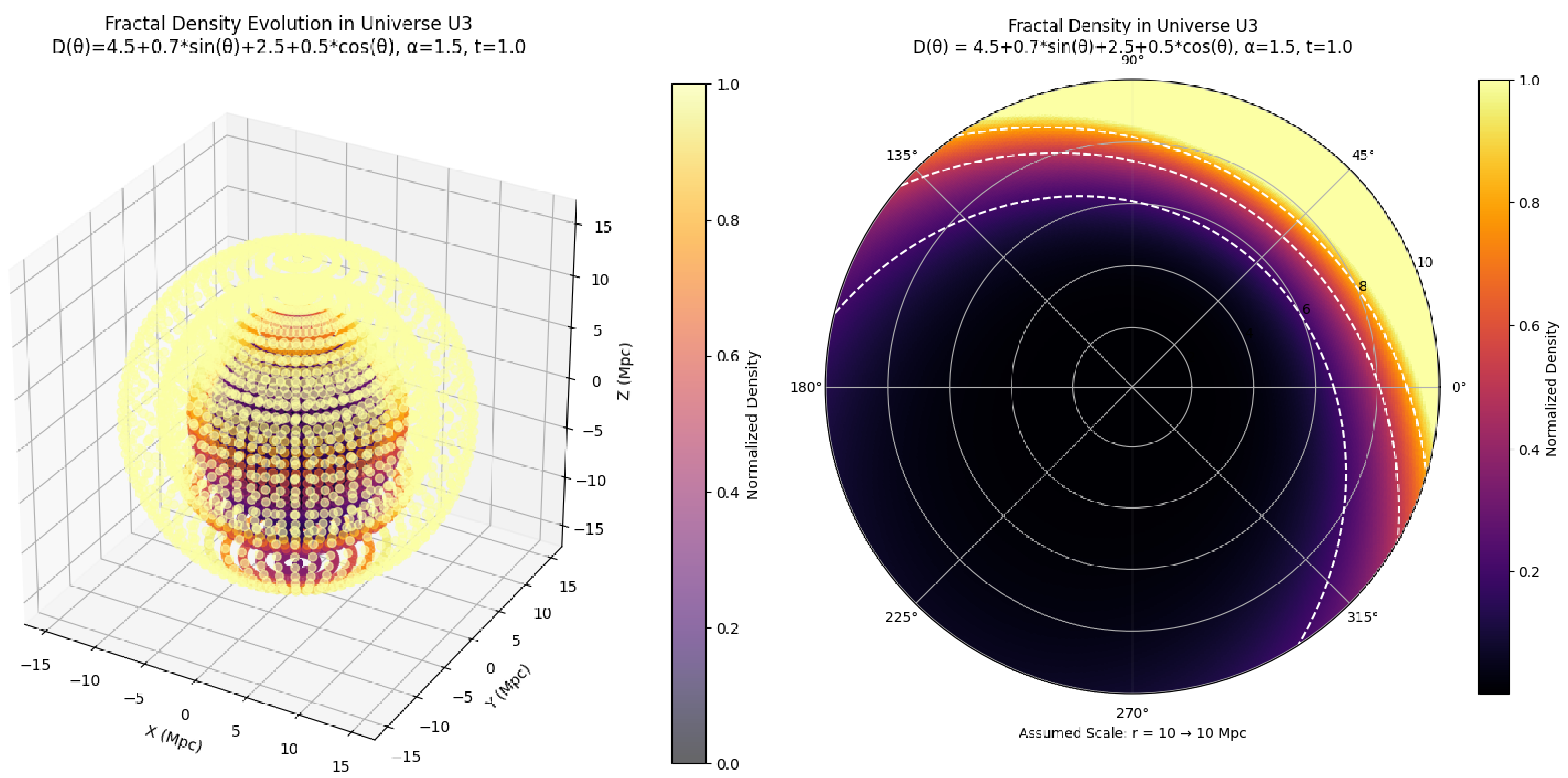
In the first transition, the parametric configuration changes to , where: Functional C is , varying in the range and Functional D is , increasing the order of the temporal derivative.
Figure 4.
Second Phase (Variation of )
The scalar field equation becomes:
The corresponding density profile now scales as to , indicating a sharp increase in density with radius. This marks a structural shift: matter begins to migrate outward, forming a dense outer shell and a sparse core. The increase in amplifies the singularity at —resulting in a more divergent behavior of the field , and associated quantities. The memory kernel now gives greater weight to near-past states, intensifying the early-time dynamics.
Consequently, the superdiffusive regime becomes stronger, accelerating the spread of matter and energy immediately after the singularity. This results in earlier and more intense shell-like structure formation [24]. While anisotropy persists due to -dependent , the dominant effect is the radial gradient in density, overshadowing directional variations.
The final phase involves a transition to , where: Functional E is defined as . This function varies between and , excluding singular points at due to the term. Functional F is , further increasing the fractional temporal order. The scalar field equation is now:
This results in a density profile scaling as to , signifying an extremely steep radial increase. The high fractal dimension, exceeding physical three-dimensionality, implies a hyper-compact, self-similar geometry at all scales. The increased causes an even more pronounced singularity at , leading to an instantaneous and violent divergence in field behavior. The memory effects now span a longer temporal domain, meaning the field evolution is strongly shaped by its deep past.
Figure 5.
Third Phase (Variation of )
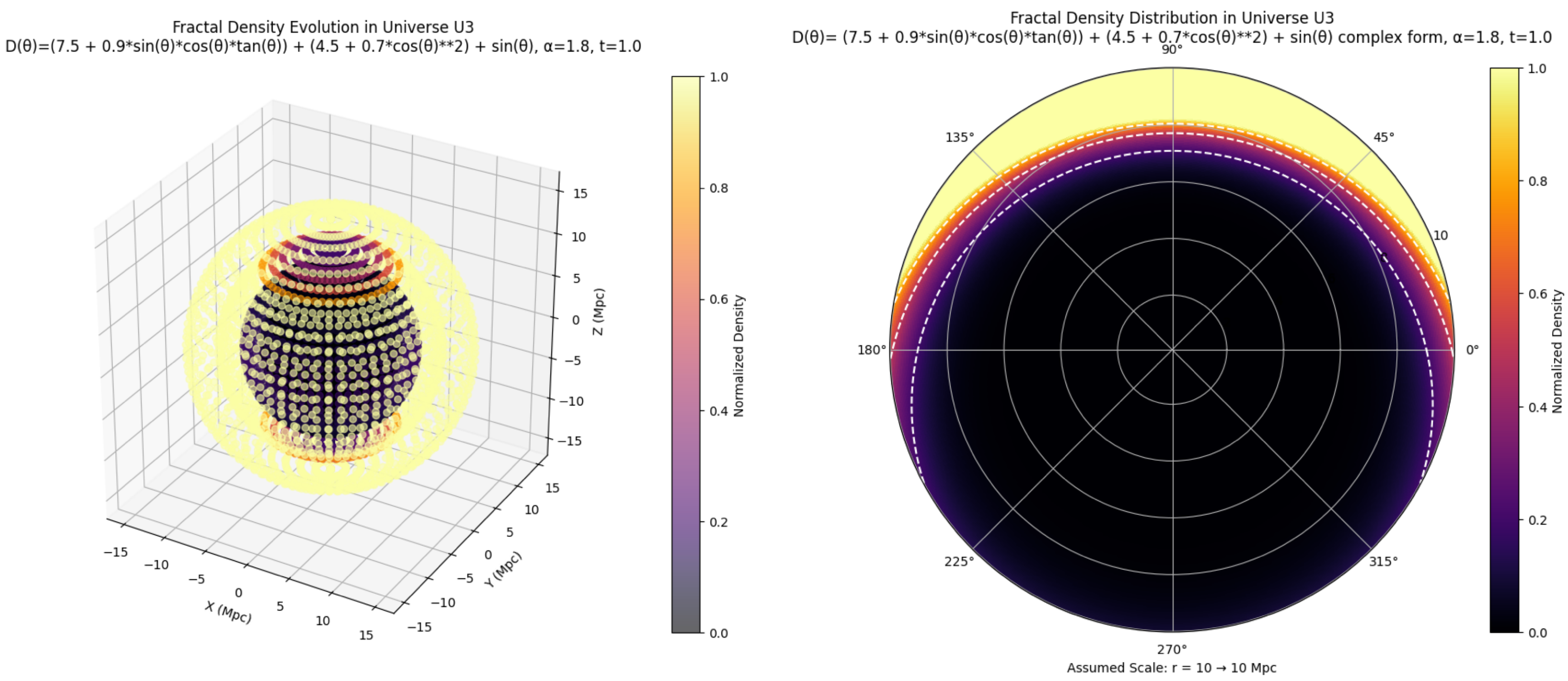
The result is an almost instantaneous restructuring: matter is rapidly expelled to large radii, leaving the core virtually empty and forming a hyper-dense outer shell. The anisotropy induced by still leads to directional shell thickness variation, but the overall impact is a nearly universal outer shell with very sparse interiors. The universe thus reaches an extreme state far more quickly than in earlier phases.
The key difference between this model—where varies—and the previous one with constant fractional order lies in the temporal dynamics and singularity structure. When remains constant, evolution is steady, and structural changes emerge more gradually. In contrast, varying not only sharpens the initial singularity but also significantly accelerates the universe’s evolution, reshaping matter distribution at each stage with increasing intensity.
In the variable- model, the growth of the parametric universe is governed not by standard expansion, but by a restructuring of spatial matter distribution, driven by both the increasing fractal dimension and fractional-order memory effects. Temporal evolution becomes progressively faster and more singular, while spatial structure shifts from moderate anisotropy to extreme radial dominance, culminating in a universe with an empty core and hyper-dense periphery—an entirely novel cosmological architecture shaped by fractional and fractal physics [3,4,14].
2.2. Building a Weird Zeta () Function Based Parametric Universe
A parametric universe, denoted as , represents a highly abstract and mathematically sophisticated cosmological model, surpassing previously described parametric universes in its structural rigor. The purpose of examining this model is twofold: (a) to rigorously justify the fundamental principle upon which the entire model is constructed at the highest level of abstraction, and (b) to investigate the extent to which the modeling of a parametric universe influences the resulting conformational variability graph and its associated consequences. The fundamental motivation for introducing this function lies in its incorporation of several intriguing aspects of mathematics—such as prime numbers, Carmichael numbers, and certain abstract equations [21,22]—which are implemented within the framework of the model. The objective is to test and explore whether, through such abstract mathematics, it is possible to construct a hypothetical universe that may not exist in its entirety, yet could potentially provide explanatory insight into certain aspects of our own universe.
This parametric universe is composed of four distinct phases, each governed by a unique parametric function derived from four different variants—termed versions—of a peculiar zeta functional. These functionals define the density profiles for each phase and act as the primary drivers of structure formation and cosmological evolution within the universe.
We begin by presenting a generalized form of the weird zeta () function along with the associated terminology:
Here, , which represents the product of twin primes. The summation runs over all such twin prime pairs. For example, , , and so on [36]. These products are summed accordingly. The constant C denotes a Carmichael number, fixed at for computational simplicity [22,23]. The set includes all prime numbers greater than 2. The symbol represents a fixed composite number (set to 4), and denotes a perfect number (set to 6). Variables X and Y are considered such that X is a real number and Y is its complex counterpart (e.g., if , then ).
We define a function that generates different equations using the variables . To formalize this system, let us introduce a machine M, which operates as follows. There are two classes of inputs: Class A, consisting of two variables , and Class B, consisting of two variables . These inputs can enter the machine in four distinct ways:
1. one variable from Class A with one variable from Class B,
2. two variables from Class A with one variable from Class B,
3. one variable from Class A with two variables from Class B, and
4. two variables from Class A with two variables from Class B.
These cases can be represented as:
Now, consider the input space as a disjoint union defined by:
where denotes the set of all possible outputs (How this operator produces such an output is not of primary importance for our analysis; therefore, we assume it functions as intended and provides the required output). Then, there exists a function
where M is a set of operators. Explicitly, we obtain:
This can be compactly expressed as:
Next, we define the operator , which acts on these input variables and produces outputs denoted by . Consider one such case k, where we define a function
which governs the initial phase and is given by:
Substituting this into the generalized form yields the final expression for the weird zeta function in the initial phase:
For the first summation term , with and , we consider the twin primes [36]. Accordingly, we compute:
Next, we evaluate the second term in the generalized function for all primes N up to 29. The expression for k is given by:
Substituting the values, we obtain: This simplifies to approximately . To evaluate the exponential term, we compute the magnitude of k, yielding . Therefore,
Now, considering , the term becomes . Summing over all primes less than or equal to 29 yields an approximate value of 255.5, which we round to 255 for simplification. Denoting this as , and using the previously calculated , we obtain: We now move to the first phase, defined by the following expression:
The first term remains the same as in the initial phase: . For the second term, we calculate: This results in: Due to the extremely large magnitude of the numerator, the value of becomes very large, making . Consequently, each term in the summation over N becomes simply , and the sum over all such is 129. Hence, Next, we consider the second phase, defined as:
The first term remains . Evaluating the expression for k, we have: This simplifies to: Thus, is an extremely large number and , leading again to each term becoming simply N. Hence, the sum remains 129, and:
Finally, we analyze the third phase, denoted as , which is given by:
We compute the value of k using:
Substituting the approximated values, the numerator becomes approximately 101 and the denominator approximately 900, resulting in:
Using this, the contribution from each term in the second summation becomes significant. After computing the summation over all primes up to 29, the total is found to be approximately . With the constant first term , we obtain:
Having established the values for all functions, we now proceed to construct a model for the density profile that captures the cosmological structure and evolution of a parametric universe [25,26]. This density profile is designed to incorporate a parametric function, with serving as amplitudes for perturbations that reflect their mathematical significance in shaping spatial structure formation across distinct phases of the universe.
We define the general form of the density profile as:
Here, the sinusoidal term introduces periodic variations that align with the structured, oscillatory nature of the -function’s exponential components. This formulation generates a shell-void pattern that evolves with the phase-dependent . The operation ensures physical plausibility by preventing negative densities.
The background density scales as , where a is the scale factor [25], accounting for the universe’s expansion and its effect on the average density over time. The perturbation term, , introduces density contrasts modulated by , directly linking the mathematical output of the -functionals to large-scale cosmological structure. With , the sinusoidal function introduces a spatial periodicity of one unit, resulting in overdensity peaks at , and voids at , inspired by the oscillatory behavior inherent to -function exponents. Since , the sinusoidal term exhibits a periodicity of one unit.
In the initial phase, where , the density profile becomes:
Figure 6.
Evolution of – Initial Phase
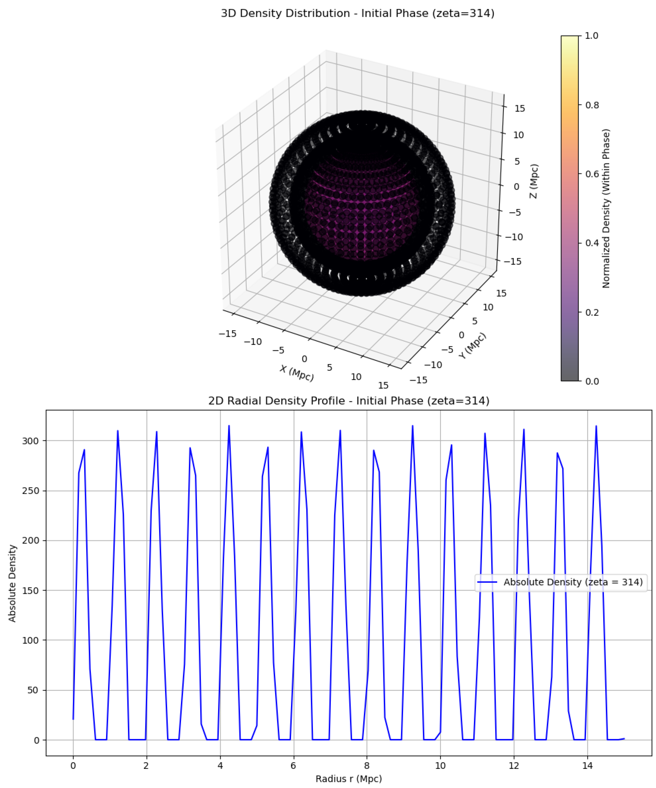
This leads to a density ranging from 0 (at minimum) to (at peak). Overdensity peaks occur at , while voids occur at , where the density drops to zero. The transition points between shells and voids occur at , where . In this phase, extremely high-density shells are formed due to the large value of , with the density contrast increasing up to 315 times the background value at the shell peaks. This significant contrast enhances gravitational collapse within overdense regions, potentially forming highly compact structures such as ultra-dense proto-galactic cores or black hole-like objects [29,30]. Voids, meanwhile, are perfectly empty and slightly narrower, occurring when , which sharpens the transition from void to shell. The periodic shell-void structure is maintained, but the increased density results in more sharply defined and compact shells. As continues to decrease with cosmic expansion, the absolute density reduces; however, the relative contrast remains high, sustaining structurally well-defined features.
Unlike models governed by fractional dynamics, the evolution of the system is dictated by a scalar field [7,28], with dynamics given by:
This scalar field equation governs the temporal and spatial evolution of , which in turn influences the universe’s expansion and thereby the background density . A first-order time derivative is employed to ensure a smooth, non-singular evolution, placing emphasis on the influence of the -function-driven density profile.
The potential is a simple quadratic form, appropriate for a matter-dominated universe [7,31] without inflationary or cyclic dynamics, ensuring a stable and gradual evolution of . The term acts as a restoring force, promoting oscillatory behavior or roll-down dynamics for , which in turn influences the Hubble expansion via the Friedmann equations [25,32].
The spatial diffusion term smooths out local fluctuations in over time, indirectly modulating density evolution by coupling the scalar field to the energy content of the universe. The small mass ensures a slow evolution of , which avoids rapid changes that could obscure the structural transitions driven by . This modeling choice emphasizes the structural effects encoded in the density profile, allowing the impact of the -dependent perturbations to dominate the cosmological dynamics during the initial phase.
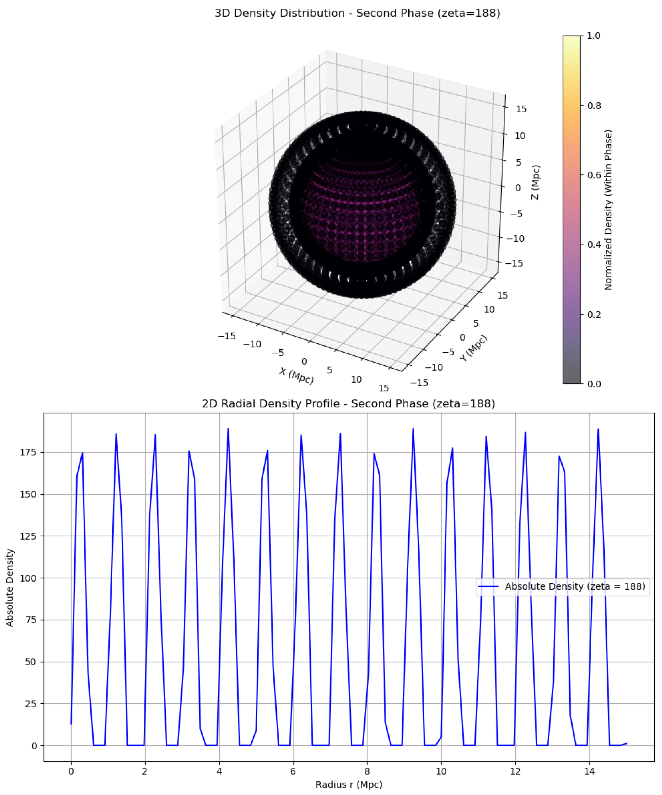
In the first phase, the density profile is defined as:
This profile yields a density range from 0 to , with a minimum (void) at and peaks at , where the density reaches . The transition points, where , occur at .
Figure 7.
Evolution of – First Phase

Compared to the initial phase, where , this phase exhibits a reduced density contrast—from 315 to 189—a drop to approximately 60 percent of the initial contrast. Despite this reduction, the shells remain significantly denser and more compact, with less softening. This persistence in high density suggests that structures formed during the initial phase do not relax substantially, maintaining their compactness and potentially resisting gravitational redistribution more effectively. Voids in this phase broaden slightly, as they occur when , implying an expansion in the void regions. Although the shell positions remain unchanged, the increased contrast sharpens the shell definition. The reduced softening effect means the universe retains much of its early extreme structure, characterized by denser shells and broader voids. The transition from void to shell is less dramatic, preserving the compact morphology of the shells well into this phase.
During the second phase, where remains constant, the density profile continues as:
This stabilization of sustains the structural configuration established in the first phase. Shells maintain a density contrast of 189, and voids remain slightly larger. The periodic shell-void pattern persists, and although decreases with cosmic expansion, the relative density contrast remains pronounced. The initial amplification from imprinted extreme structures early in the universe, with dense shells prone to collapse into compact objects, enhancing early cosmic lumpiness.
Figure 8.
Evolution of – Second Phase
The transition from to results in a less dramatic reduction in density contrast, suggesting that much of the initial extreme structure persists into the first phase. These denser shells resist softening, maintaining a pronounced shell-void pattern throughout cosmic evolution. The slightly more expansive voids enhance the visual contrast between dense shells and empty regions, imparting a more ’hollow’ appearance to the universe at large scales. By the end of this phase, the stabilized structure features high-density shells and expanded voids, resulting in a mature cosmological configuration.
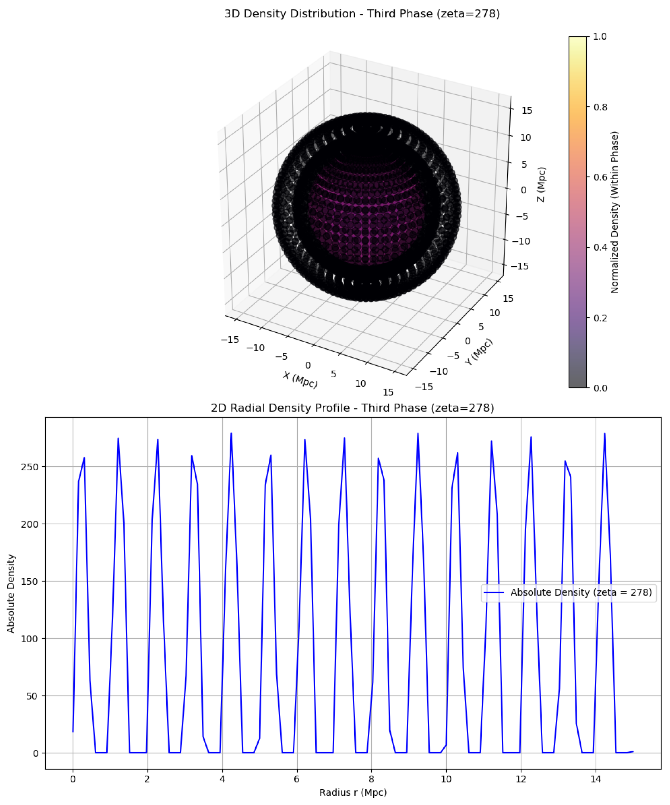
In the third phase, the density profile evolves as:
Since , the sinusoidal term oscillates with a period of one unit, producing density peaks at and troughs at . The background density evolves as , consistent with a matter-dominated universe where [25,28]. The density profile in this phase spans from 0 to , with voids occurring where , indicating slightly narrower void regions.
Compared to the second phase, the density contrast increases by approximately 47.6 percent, rising from 189 to 279. This re-densification tightens the shell structures, making them more compact and approaching the extreme densities seen in the initial phase. The enhanced density supports stronger gravitational collapse within the shells, potentially leading to the formation of denser, more concentrated structures—possibly manifesting as tightly packed, spherical walls of matter [25,26].
While voids at remain effectively empty, their slight reduction in width sharpens the transition into dense shells. Consequently, shells become more distinctly defined, and the density contrast drives a further maturation of the universe’s structural features [25,27]. This phase deepens the shell-void morphology established earlier, reinforcing the universe’s layered architecture with compact, high-density shells and increasingly isolated voids.
The evolutionary impact of the third phase is profound, marking a significant re-densification that more aggressively reverses the softening trend observed in previous phases. Shells that had gradually relaxed during the first and second phases now contract and become increasingly dense and compact, as if the universe is undergoing a phase of structural recompression. Although the background density continues to decrease due to cosmic expansion, the relative density contrast increases, rendering the shell-void pattern more pronounced [7,28]. This enhanced contrast signifies that, despite the drop in absolute density, the visual and gravitational significance of the structures becomes more prominent.
Figure 9.
Evolution of –Third Phase
The strength of this re-densification in the third phase makes it a dramatic recompression stage, drawing the shell densities closer to the extreme contrast values seen in the initial phase. As a result, the universe evolves toward a final structural state that is nearly as sharply defined and contrast-rich as its early configuration.
The progression across phases in this parametric universe—characterized by an initial phase of extreme density, followed by structural softening, then stabilization, and finally strong re-densification—resembles a cycle-like evolution in structure, even though the underlying universe itself is not cyclic. This structural trajectory, culminating in the third phase, suggests a return to a high-contrast state, implying that the universe’s morphology oscillates between extreme and relaxed regimes before settling into a dense and ordered configuration. Such a progression underlines a dynamic evolution where mathematical parametrization, through the values, orchestrates shifts in the cosmic density landscape without invoking traditional cyclic cosmology [33,34].
We can now extend this analysis to different instances of k, i.e., equations generated from , and embed them within our -function framework to obtain various outputs such as:
The operator is thus capable of generating infinitely many such equations through the application of very simple rules and only four variables. The central purpose of introducing this function is to demonstrate how, starting from simple variables and minimal rules, one can construct a system of remarkable complexity, capable of modeling the evolution of a universe. Each such universe will possess distinct structural properties and exhibit unique patterns of overall evolution.
2.3. Comparative analysis of the Universe and
Parametric Universe (a fractal universe) is constructed using fractal dynamics to define its density profiles and govern the overall structural evolution of the cosmos. In contrast, Universe introduces the unconventional -functional to drive its formation and evolution. These two parametric universes are fundamentally distinct in both mathematical foundation and structural behavior. A concise comparison of their core features provides a clear framework for further analysis.
In the case of , the structural evolution is characterized by hierarchical and anisotropic growth. During the early stages, the influence of fractional dynamics with results in a slower initial evolution of the scalar field , thereby delaying the onset of structure formation [15,35]. The density profile remains low at small radial distances, leading to sparse early structures near the center [3]. As the universe evolves into the intermediate stage, the density increases rapidly with radius, forming overdense regions on larger scales. The angular dependence embedded in introduces anisotropy, with structures preferentially forming in regions where attains higher values [4,5]. Consequently, large-scale structures dominate in these directions, giving rise to clusters and filaments. The fractal nature of ensures self-similarity, where smaller structures are nested within larger ones [4,6], yet the overall distribution remains highly anisotropic due to the directional variability in fractal dimension.
On the other hand, exhibits a periodic and isotropic structure, particularly evident in its initial phase. Here, extreme density contrasts generate compact spherical shells located at , separated by sharply defined voids, resulting in a highly ordered configuration resembling a lattice of concentric shells. During the first phase, a softening occurs, reducing the density contrast to 189 and rendering the shells more diffuse with broader voids [27]. In the second phase, the structure stabilizes while maintaining its periodic pattern, but the density contrast remains unchanged. The third phase introduces a re-densification process, increasing the contrast to 279, which tightens the shells and brings their compactness closer to the extreme density of the initial phase. Throughout all phases, the structure of remains isotropic and periodic, with the shell-void pattern consistently defined by the sinusoidal profile [25,26].
3. On Philosophical Consequences of Abstract Universes
Mathematics lies at the very heart of science. It is the universal language that transcends space and time. The universes constructed on paper are often highly abstract, yet they remain mathematically consistent. The central question, then, is: Do such universes possibly exist? To interpret this question, we must carefully examine every aspect of it. What do we mean by universe? This becomes the central theme of the present work. The abstract universes we construct serve to justify and probe this very argument—namely, what we truly mean when we use the term universe.
The Platonic view provides a cornerstone argument in this regard [11,12,41]. If the Platonic perspective is correct, then mathematical entities and forms exist independently of us, and our comprehension of them depends on the limits of human intelligence. Accepting this idea makes it more plausible to suggest that abstract mathematical universes, such as those developed here, might indeed exist. However, at present, we lack experimental verification for any such claims. To generalize this line of reasoning, we may ask: if something can be described mathematically within a valid formal framework, can it also be experimentally verified as an existent reality?
Consider, for example, the argument presented by Eugene Wigner in his seminal paper ’The Unreasonable Effectiveness of Mathematics in the Natural Sciences’:
“We make a rather narrow selection when choosing the data on which we test our theories. How do we know that, if we made a theory which focuses its attention on phenomena we disregard and disregards some of the phenomena now commanding our attention, that we could not build another theory which has little in common with the present one but which, nevertheless, explains just as many phenomena as the present theory? It has to be admitted that we have no definite evidence that there is no such theory.”[10]
Our interpretations are always rooted in the axioms and assumptions that allow us to construct frameworks. For instance, consider the fractal universe . Based on current observational data, the universe as a whole is not identical to a fractal universe. However, there remains a (perhaps small) probability that certain regions of our universe, as yet undiscovered or unobserved, might exhibit behaviors resembling—though not identical to—those described by the fractal universe [4,6]. This suggests that while the universe in its entirety may not conform to such a model, abstract universes built from specific mathematical functions may nonetheless capture aspects of reality, even in domains for which they were not originally constructed. In this sense, the fractal universe may provide insights into regions of our cosmos that are not themselves fundamentally fractal, yet behave in ways that align with its mathematical structure [3].
Interpretations used to describe any phenomenon are inherently flawed, as they are grounded in the observational standpoint and pattern-articulation capabilities of the respective species. The key idea here is that humans possess a remarkable ability to articulate patterns. However, it is essential to be precise when asserting that humans are “good” at articulation and comprehension. Specifically, we must define what is meant by the “way” of articulation. This refers to the algorithmic paradigm governing how a species articulates patterns and perceives reality. Such paradigms may differ radically across species. Some species may possess entirely different mechanisms for pattern articulation and interpretation. If that is the case, does it imply that the laws of nature manifest differently for them?
One hypothesis is that our inherent ability to articulate patterns enables us to construct a vivid and complex conception of reality. The act of questioning itself—our capacity to formulate and pursue questions—may be the very foundation of the diversity within the perceived reality that we described earlier. The central idea I propose and wish to elaborate on is that any rigorous formal system—constructed with axioms, derived theorems, and base assumptions—ultimately falls into the domain of pure abstract mathematics and logic and is fundamentally confined. This confinement stems from the fact that any such formalized system, no matter how abstract or rigorous, is still a product of the articulation of patterns. And this articulation is in turn constrained by the algorithmic paradigm of the species constructing it.
In other words, abstraction itself is a byproduct of pattern articulation, and any system built upon such abstraction inherently carries fundamental limitations. The interpretations, meanings, and languages derived from these systems are shaped by the underlying algorithmic paradigm unique to each species. When viewed across paradigms, these systems often appear inherently chaotic or incompatible. The algorithmic paradigm constitutes the core mechanism by which articulation occurs, and it governs how such articulation can be extended, modified, or manipulated. Consequently, any attempt to assert the universality of a system developed within a single paradigm must be approached with caution, as it may lack meaningful correspondence with the structures of reality as perceived and constructed by other paradigms.
One of the main reasons for this paper is to understand the profoundness of mathematics as a whole—how effectively it can be used and interplayed to understand the complexity of the world. One important aspect in this context is the idea described in Wigner’s paper [10]. Let us suppose there exists a mathematical framework that describes a system S. Now, there is a non-zero probability that another mathematical framework could also explain the same system. In such a case, the idea of effectiveness is not central, since both frameworks effectively explain the system. If one argues that one theory explains the system more simply compared to the other, then this reflects not effectiveness but rather simplification of the argument. Both frameworks remain effective. This brings us to the core reasoning: if another framework can describe system S, then more than two theories could potentially exist to explain the same system. The question then arises—how many such frameworks are possible in this scenario, and are all of them valid?
4. The Mosaic Patchwork Hypothesis
When we consider the two hypothetical universes, and , it becomes evident that they do not represent our universe in its entirety. However, if we focus on a very small portion of the universe, we may attempt to observe the evolution of its structure and compare it with the evolutionary paths of these hypothetical universes. There exists a non-zero probability that the evolution of such universes might, in some way, coincide with our own.
Here is the hypothetical idea: imagine dividing our universe U into different regions, each with a defined dimension and cubic volume, denoted as . While n could, in principle, be infinite, to keep the argument less complicated we will assume n is finite.
Now, to proceed clearly, we define a few assumptions which are crucial and central to our argument:
1. Our universe is divided into cubic volumes,
2. There exist corresponding hypothetical universes,
each with its own mathematical framework to describe the universe. This can be represented completely as
3. The most important of all assumptions: these hypothetical universes will not necessarily explain or describe our universe as a whole, but only a fraction of it at a given frame .
With these assumptions, each such hypothetical universe can effectively describe the evolution or structure of one particular cubic region of the universe, though not the entire universe. In other words, a given hypothetical universe may account for the structure, evolution, or phenomena of a specific celestial region.
Thus, for each of the n cubic volumes, we could have n corresponding hypothetical universes that provide explanatory frameworks for those regions. Does this imply that within such a complex mathematical paradigm, we may construct as many frameworks as needed — some of which explain certain physical aspects of reality while others remain abstract and less relevant? Importantly, the lack of universal applicability does not mean these frameworks are illogical or inconsistent. Rather, they may remain abstract in some regions, while in others they can successfully predict, explain, or resemble aspects of physical reality.
Let us now take the argument one step further. If there exist n cubic volumes, each with n corresponding hypothetical universes, and if some of these evolutionary descriptions resemble aspects of our own universe, does this imply that we require n such theories to fully explain our universe as a whole?
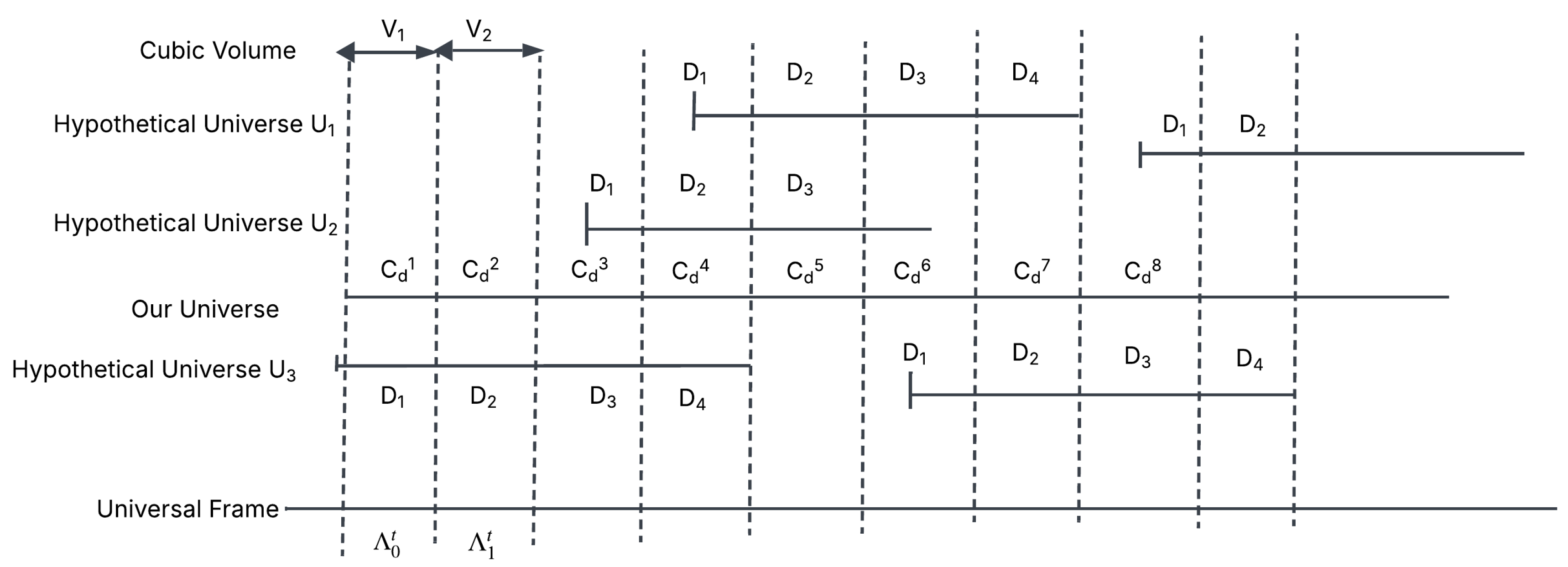
To sharpen this argument, let us narrow it down to a simpler case. Suppose we divide the universe into four cubic volumes, denoted as , and consider eight different hypothetical universes, (with particular attention to and , as discussed in the paper).
Now, let us define a concept called the universal base clock, denoted as , where . This represents a universal measure of time. For example, at , which we consider as the initial frame of space-time, each universe describes a defined scenario within one cubic volume: describes the defined scenario of , describes that of , of , and of .
Moving forward, it is also possible that at the next frame, , other universes describe these volumes differently: for instance, might describe , describe , describe , and describe . This process can continue across successive frames, where at each , different universes among the eight may provide the explanation for a given cubic volume.
At this point, let us also introduce the notion of defined scenarios. Corresponding to the hypothetical universes, these scenarios are represented as , with each describing the outcome or structure provided by its respective universe. Corresponding to our actual universe, however, we define a composite defined scenario, denoted as , which integrates the descriptions of the cubic volumes at each frame.
For example, at , universe may describe cubic volume with defined scenario of , while at the same time contributing to the composite scenario of our universe . At the next frame, , the same universe may describe cubic volume with defined scenario of , and this would then contribute to the composite scenario of our universe .
Here we must note two possibilities for analysis:
Single-framework condition (restricted case): At any given frame , only one hypothetical universe contributes the defined scenario for a cubic volume. This simplifies the mapping and avoids complications.
Multiple-framework condition (general case): At any given frame , multiple hypothetical universes may yield the same defined scenario for a cubic volume. In this case, the mapping becomes many-to-one, and equivalence across different frameworks emerges naturally.
The central idea is that with each frame change, the universe responsible for explaining a particular cubic volume may differ. We can imagine this mathematical framework as a line segmented into many parts, with each part being useful for describing certain scenarios at specific frames for specific cubic volumes.
Moreover, because there are more possible defined scenarios than cubic volumes (), redundancy arises naturally: equivalent scenarios can appear at different times or be explained by different universes. For example, suppose a defined scenario occurs in cubic volume , described by at frame . Then, at another frame, , an equivalent scenario (where ) may occur in cubic volume , this time described by .
With this reasoning in place, multiple interpretations and extensions of the argument can be developed.
Figure 10.
The conceptual diagram of the Thought Experiment
We begin by defining
as the set of cubic regions of our universe. Let
denote the set of frames, where each frame is written as
In particular, the universal frame can be expressed as
meaning the first frame starts at 0.
Now, let
be the set of hypothetical universes, and let
be the set of mathematical frameworks corresponding to these hypothetical universes.
Next, let D denote the set of possible defined scenarios — atomic local outcomes that correspond to structures, processes, events, and evolutions within hypothetical universes. We assume D is finite, so that
Accordingly, there are n such defined scenarios. We then define a composite defined scenario, which represents essentially the same class of defined scenarios but distinguished from the hypothetical-universe-specific ones by using the term composite. This is given as
which we also assume to be finite.
For each universe , we define a function
such that gives the defined scenario that predicts for region at frame T, under its corresponding mathematical framework . In other words, encodes the full local description or prediction that assigns to any region and frame.
We now introduce the composite defined scenario of our universe. This is described by the map
where represents the actual defined scenario of our universe at region and time frame T.
The key relation between and C is as follows: for each , there exists at least one
such that
That is, at every location and time frame, the actual scenario coincides with the scenario given by at least one hypothetical universe.
There are two possible cases in this thought experiment. In the first case, only one hypothetical universe describes the local cubic volume at a given frame. In this situation, there exists a function
such that for every :
Thus, exactly one universe describes that region of our universe at the given frame.
In the second case, more than one hypothetical universe describes the same cubic volume at a given frame. For this, we define a relation
such that for each , the nonempty set
is precisely the set of universes whose descriptions agree with C at that frame. Formally,
and this set may have cardinality .
We must now consider the dynamics of how scenarios evolve over time frames, and in doing so, explain the fraction of our universe that corresponds to each. At time frame , suppose a hypothetical universe , with mathematical framework , successfully describes the defined scenario of region . At the next frame, however, it is possible that a different hypothetical universe , with framework , may instead describe the evolution of that same region . In other words, the responsibility for explaining the defined scenario of a given region can shift from one hypothetical universe to another as time progresses, although it may also remain with the same universe.
Moreover, in cases where more than one hypothetical universe provides a valid description of the same cubic region at a given frame, we require a mechanism — a kind of selection machine — that takes as input the set of hypothetical universes (each with its mathematical framework and corresponding defined scenarios), examines their predictions at that frame, and then assigns to each cubic region the defined scenario from whichever universe coincides with our own universe’s evolution.
Thus, at any given time frame T, the following objects are known: for each universe , its local description at , namely , as well as the composite defined scenario of the universe at time T, namely . We then define witness sets at each site as
By the hypothesis of the thought experiment, each is nonempty. In essence, is the set of witness universes for a region at time frame T: that is, all universes whose prediction matches the actual scenario at that specific cubic volume and time frame. These are precisely the indices k for which
meaning the universes that match reality at that location.
Now let us talk about the selection operator, which is defined as
where is the output of the function. To understand this, note that represents a list of all universe’s cubic region maps at time frame T. Each map specifies, for every region , what scenario universe predicts at time T. The function represents our universe’s composite defined scenario’s cubic region map at that same time. In essence, S compares the predictions from all hypothetical universes at time T with the actual observed scenarios of our universe at that same time, and then makes a selection. Thus, S takes functions as input and produces as output. Since itself is a function, the operator S effectively returns a function.
We now define as follows:
This can be understood as follows: the domain of is V, the set of cubic regions (i.e., the actual universe), and the codomain is . Here is the power set of (the set of all subsets of universes), from which we exclude the empty set . Therefore, for each region , the function returns a nonempty subset of universes. In words,
Formally,
where is the witness set, i.e., the set of all universes whose prediction or defined scenario matches reality (our universe) at region . This constraint enforces that the machine is only allowed to select universes that agree with our universe in the given region at the given time frame.
We begin with a machine which, for given inputs, produces the required output. What remains is to design a rule or mechanism that determines which subset of candidate outputs to keep and which to discard. In other words, given the input, the machine must apply an underlying principle that selects the required output, thereby explaining the cubic regions of our universe at a given frame of time.
The idea behind this mechanism is as follows: for each cube at time T, we compare the microstate distribution of our universe’s observed scenario with the corresponding microstate distributions implied by each hypothetical universe’s scenario . We then apply a similarity measure, together with entropy-based constraints, to score each universe. The machine then selects the universe(s) with the top score(s) as the admissible witness set . The selected universe’s microstate dynamics are then used to predict .
Let D denote the set of macro-defined scenarios. Each macrostate corresponds to a (possibly large) set of microstates . For our observed universe, the composite macrostate at is denoted . Its associated microstate distribution over is written as
with normalization
For a hypothetical universe , the macrostate of region at time T is
with microstate distribution
If , we map both to a common feature space (via coarse-graining, histograms, momenta, fields, etc.). From this point forward, we assume both distributions are defined on the same finite space (or ).
We require a numerical measure of closeness between and . For this we use the Bhattacharyya overlap [19]:
This equals 1 if the two distributions are identical and 0 if their supports are disjoint. Larger overlap is better.
The Shannon entropy [20] of a discrete distribution is defined as
For region at time T:
If microstate distributions are close, their entropies should also be close. We define the entropy mismatch as
where small values indicate better matches.
Each hypothetical universe specifies a dynamical law governing how microstates evolve:
At time T, universe provides not a single microstate but a distribution:
The law acts on distributions, yielding the prediction
The entropy at times T and is
The entropy change is
Physically, not all entropy changes are admissible. We therefore impose a plausibility condition, for example requiring that entropy is non-decreasing on average:
The entropy-based score is defined as
where is a sensitivity parameter. Thus, the entropy score of at cube is high if (i) its entropy matches the observed region closely, and (ii) its predicted entropy evolution is physically plausible.
This feeds into the canonical scoring rule:
where are weights that balance similarity, entropy consistency, and the penalty term , which discourages ’jumpy’ or overly complex explanations.
Recall the witness set:
The selection operator S returns
A canonical selection rule is
That is, for a cube at time T, we compute the score for every candidate universe , and select the universe(s) yielding the maximum score.
Once is selected for cube at time T, its internal evolution law determines the subsequent state:
Thus, the predicted next state of cube is
The composite predicted scenario of the universe at time is then
This provides a patchwork-style prediction of the universe’s evolution across all cubic regions.
So, now let’s say we have selected a cubic region of our universe with a defined scenario . We consider two possibilities: (i) only one hypothetical universe at time frame explains or aligns with the defined scenario of our universe’s at the cubic region ; and (ii) more than one hypothetical universe—let’s say four such hypothetical universes—align with the defined scenario of our universe at that given cubic region .
The main argument is this: if all such abstract universes exist, and we imagine that there are infinitely many such hypothetical universes instead of just some finite number n, then all of them in one way or another explain some part of our universe. We consider our universe as a reference because we do not know whether multiple universes exist or not. These abstract universes, formed out of mathematical frameworks, exist since the mathematics used to build them is consistent. That means these universes exist apart from physical reality, something like Plato’s world of forms [37]. A fraction of them, at a given frame, explains the physical reality we live in.
That is one way to argue based on the thought experiment. Another way is this: if mathematics is supposed to be the universal language to explain the universe [10], then it should have one fixed framework. But as we saw in the thought experiment, this is not the case. That means mathematics is not the universal language in the way we thought it was. Maybe it is, but in a different sense. It is not a universal language, but rather a universal space of possible languages [12]. This is very important, because it can also mean that there could exist other abstract languages which, if they exist, might validate interpretations that align with reality, or even suggest that the existence of such abstract universes is an independent reality on its own.
A third argument is this: what matters most is that mathematical abstraction connects to reality depending on the interpreter—whether it is a species or some other entity X—that is trying to comprehend it [38]. The meaning and universality of mathematics are not in mathematics alone, but come out of the interaction with the intelligence interpreting it. This makes mathematics not an absolute thing but a relational entity. This idea is important because it means that in our first argument—where we said all abstractions exist in some form—only those that connect to our physical reality appear aligned. But for that to happen we need an interpreter, like a species, to actually understand or make sense of how such frameworks are aligning with reality.
For example, in our formalization of the thought experiment, in the selection mechanism we introduce microstate distributions and entropy [20,39]. A machine could use this to maximize alignment between a cubic region of our universe and the defined scenario of hypothetical universes at that given time frame, and then choose the universe that best explains our cubic region. Now think of another way to do the same task. Again we imagine a machine, but this time instead of using microstates or entropy, it relies on the third argument. Let’s say we have four interpreters: a human, an advanced AI, an alien species, and an animal on Earth (say a dolphin). Each of them acts as the mechanism for the machine to choose the most fitting defined scenario of hypothetical universes that matches our universe’s defined scenario at the cubic region and at that time frame.
One interpretation from this is that the method or rule each of the four uses to evaluate the hypothetical universes and match them to our cubic region will be different, because it depends on how they perceive or comprehend reality. But if we consider the opposite argument—that each species, whether human, AI, alien, or animal, will always use some method that is still part of the set of all possible methods of interpretation—then it follows that there must exist some scenario where all of them could actually choose the same method and select the same hypothetical universe’s scenario for our cubic volume. How that would happen is beyond the scope of this paper. But still, the argument stands until we have a clearer understanding of what we mean when we talk about a “universe,” and also what we mean by “mathematics” itself.
From here another argument arises. It could be possible that one of the most important aspects of mathematics, or its abstraction, is that we can never really understand what it exactly means [40]. To do that, we would first have to understand where mathematics itself comes from. The problem is this: There are two possibilities: (i) Mathematics has existed since the universe came into existence [12,42]. If so, it would mean you cannot explain the universe with mathematics to such an extent, since the very language of mathematics itself arises from, or existed because of, the existence of the universe. (ii) You cannot explain mathematics using mathematics, because to do so you would have to explain its origin, and it already arises from mathematics. In simple terms, if we have x (say, a language) that originates from X (a universe here), then x cannot fully explain X, since x itself comes from X. This creates a limit of comprehension—x cannot explain X. Which means there is always an undecidability about whether x can explain X or not.
So these arguments lead us to ask whether, with such abstraction, we will ever really be able to understand the universe—or even what we mean when we say “universe.” Such questions can only be approached through more understanding and scientific development, which can help us comprehend the observational aspects of the universe. Step by step, piece by piece, we might then be able to pull out the ideas that shape our reality, and through that, move closer to understanding it.
5. Conclusions
Based on the analysis of the universes constructed in the paper and the subsequent philosophical implications, it can be inferred that there is a paradigm still beyond our view. The complex patterns and structures within the universe, and the universe itself, are fundamentally ideal, and we as a species are approaching the stage of deducing their interpretations through logical and intellectual curiosity. As Einstein famously remarked, “The most incomprehensible thing about the universe is that it is comprehensible.”[1] This profound statement reflects the essential role of mathematics and theoretical reasoning in uncovering the structure of the cosmos.
There is always a possibility that the abstraction of mathematics as a whole can never be understood as raw and truly as it is. Yet, the effectiveness of such abstraction cannot be denied, since it is profoundly accurate [10]. One of the reasons why this is the case is because we, as a species, are deeply acquainted with the patterns in nature and use abstraction to explain those patterns [38]. To understand the ontological perspective behind mathematics, we need to understand where it came from. It could also be a possible interpretation that mathematics is a shadow of the universe’s structure rather than its essence [11,37]. However, it can be firmly stated that the limitations of such abstractions are not technical but rather fundamental, and tied to undecidability—whether mathematics can be explained in the same way that we use mathematics to explain the world [40].
The foundational principle upon which the entire model rests must be defined with clarity and precision. Such precision is necessary not only to demonstrate the importance of establishing a well-defined principle in any theoretical model, but also to enable a deeper and more accurate interpretation of the model’s scope and structure.
References
- Einstein, A. Physics and Reality. Journal of the Franklin Institute 1936, 221(3), 349–382. [Google Scholar] [CrossRef]
- Hawking, S. Black Holes and Baby Universes and Other Essays; Bantam Books, 1993. [Google Scholar]
- Mandelbrot, B. B. The Fractal Geometry of Nature; Macmillan, 1983. [Google Scholar]
- Pietronero, L. The Fractal Structure of the Universe: Correlations of Galaxies and Clusters and the Average Mass Density. Physica A 1987, 144(2–3), 257–284. [Google Scholar] [CrossRef]
- Coleman, P.; Pietronero, L. The Fractal Structure of the Universe. Physics Reports 1992, 213, 311–389. [Google Scholar] [CrossRef]
- Labini, F. S.; Montuori, M.; Pietronero, L. Scale-invariance of galaxy clustering. Physics Reports 1998, 293(2), 61–226. [Google Scholar] [CrossRef]
- Mukhanov, V. Physical Foundations of Cosmology; Cambridge University Press, 2005. [Google Scholar]
- Planck Collaboration. Planck 2018 results. VI. Cosmological parameters. Astronomy & Astrophysics 2020, 641, A6. [Google Scholar] [CrossRef]
- Russell, B. A History of Western Philosophy; Simon and Schuster, 1945. [Google Scholar]
- Wigner, E. P. The Unreasonable Effectiveness of Mathematics in the Natural Sciences. Communications on Pure and Applied Mathematics 1960, 13(1), 1–14. [Google Scholar] [CrossRef]
- Tegmark, M. The Mathematical Universe. Foundations of Physics 2008, 38(2), 101–150. [Google Scholar] [CrossRef]
- Tegmark, M. Our Mathematical Universe: My Quest for the Ultimate Nature of Reality; Knopf, 2014. [Google Scholar]
- Falconer, K. J. Fractal Geometry: Mathematical Foundations and Applications; Wiley, 2004. [Google Scholar]
- Tarasov, V. E. Fractional Dynamics: Applications of Fractional Calculus to Dynamics of Particles, Fields and Media; Springer, 2011. [Google Scholar]
- Tarasov, V. E. Fractional systems and fractional Bogoliubov hierarchy equations. Physics of Plasmas 2005, 12(8), 082106. [Google Scholar] [CrossRef]
- Podlubny, I. Fractional Differential Equations; Academic Press, 1999. [Google Scholar]
- Applications of Fractional Calculus in Physics; Hilfer, R., Ed.; World Scientific, 2000. [Google Scholar]
- Kilbas, A. A.; Srivastava, H. M.; Trujillo, J. J. Theory and Applications of Fractional Differential Equations; North-Holland Mathematics Studies; Elsevier, 2006; Vol. 204. [Google Scholar]
- Bhattacharyya, A. On a measure of divergence between two statistical populations defined by their probability distributions. Bulletin of the Calcutta Mathematical Society 1943, 35, 99–109. [Google Scholar]
- Shannon, C. E. A Mathematical Theory of Communication. Bell System Technical Journal 1948, 27(3), 379–423. [Google Scholar] [CrossRef]
- Hardy, G. H.; Wright, E. M. An Introduction to the Theory of Numbers, 5th ed.; Clarendon Press, Oxford, 1979. [Google Scholar]
- Ribenboim, P. The New Book of Prime Number Records; Springer, 1996. [Google Scholar]
- Korselt, A. “Problème chinois,” translated note introducing Korselt’s criterion for Carmichael numbers (Historical source). 1899. [Google Scholar]
- Zeldovich, Y. B. Gravitational instability: an approximate theory for large density perturbations. Astronomy and Astrophysics 1970, 5, 84. [Google Scholar]
- Peebles, P. J. E. Principles of Physical Cosmology; Princeton University Press, 1993. [Google Scholar]
- Coles, P.; Lucchin, F. Cosmology: The Origin and Evolution of Cosmic Structure, 2nd ed.; Wiley, 2002. [Google Scholar]
- Springel, V.; et al. Simulations of the formation, evolution and clustering of galaxies and quasars. Nature 2005, 435, 629–636. [Google Scholar] [CrossRef]
- Kolb, E. W.; Turner, M. S. The Early Universe; Addison-Wesley, 1990. [Google Scholar]
- Rees, M. J. Black hole models for active galactic nuclei. Annual Review of Astronomy and Astrophysics 1984, 22, 471–506. [Google Scholar] [CrossRef]
- Carr, B. J. The primordial black hole mass spectrum. The Astrophysical Journal 1975, 201, 1–19. [Google Scholar] [CrossRef]
- Linde, A. D. Chaotic inflation. Physics Letters B 1983, 129(3–4), 177–181. [Google Scholar] [CrossRef]
- Friedmann, A. Über die Krümmung des Raumes. Zeitschrift für Physik 1922, 10, 377–386. [Google Scholar] [CrossRef]
- Steinhardt, P. J.; Turok, N. A cyclic model of the universe. Science 2002, 296(5572), 1436–1439. [Google Scholar] [CrossRef]
- Novello, M.; Bergliaffa, S. E. P. Bouncing cosmologies. Physics Reports 2008, 463(4), 127–213. [Google Scholar] [CrossRef]
- Zaslavsky, G. M. Chaos, fractional kinetics, and anomalous transport. Physics Reports 2002, 371(6), 461–580. [Google Scholar] [CrossRef]
- “Twin primes,” a placeholder reference on twin prime statistics—use appropriate number theory source.
- Plato. 1997, Complete Works, ed. J. M. Cooper, Hackett Publishing. (Includes Republic and the theory of forms).
- Lakoff, G.; Núñez, R. Where Mathematics Comes From: How the Embodied Mind Brings Mathematics into Being; Basic Books, 2000. [Google Scholar]
- Boltzmann, L. Über die Beziehung zwischen dem zweiten Hauptsatze der mechanischen Wärmetheorie und der Wahrscheinlichkeitsrechnung, respektive den Sätzen über das Wärmegleichgewicht. Sitzungsberichte der Kaiserlichen Akademie der Wissenschaften Wien 1877, 76, 373–435. [Google Scholar]
- Gödel, K. Über formal unentscheidbare Sätze der Principia Mathematica und verwandter Systeme I. Monatshefte für Mathematik und Physik 1931, 38, 173–198. [Google Scholar] [CrossRef]
- Laughlin, G.; Bodenheimer, P.; Adams, F. C. The end of the main sequence. The Astrophysical Journal 2000, 540(1), 288–302. [Google Scholar] [CrossRef]
- Putnam, H. 1975, “What is Mathematical Truth?” Mathematics, Matter and Method, Cambridge University Press. (See also Penrose, R. 1991, The Emperor’s New Mind, Oxford University Press, for a Platonist view).
Disclaimer/Publisher’s Note: The statements, opinions and data contained in all publications are solely those of the individual author(s) and contributor(s) and not of MDPI and/or the editor(s). MDPI and/or the editor(s) disclaim responsibility for any injury to people or property resulting from any ideas, methods, instructions or products referred to in the content. |
© 2025 by the authors. Licensee MDPI, Basel, Switzerland. This article is an open access article distributed under the terms and conditions of the Creative Commons Attribution (CC BY) license (http://creativecommons.org/licenses/by/4.0/).
Copyright: This open access article is published under a Creative Commons CC BY 4.0 license, which permit the free download, distribution, and reuse, provided that the author and preprint are cited in any reuse.


