
Submitted:
17 September 2025
Posted:
17 September 2025
You are already at the latest version
Abstract
We ask how Lorentzian causal structure can emerge from a pregeometric substrate. For a rigorously defined class of finite–range, ferromagnetically coupled “chronon” models with quartic norm pinning, we prove the existence, with strictly positive Gibbs probability, of a macroscopic percolating domain \(D\subset M\) on which the coarse–grained field \(\Phi^\mu\) is smooth, future–directed, unit–norm timelike (\(\Phi^\mu\Phi_\mu=-1\), \(\Phi^0>0\)) and twist–free. We work on a smooth differentiable manifold but do not assume Lorentzian signature or a global time field a priori; these arise on \(D\) from the dynamics.Under four operational axioms—well-posed local dynamics, finite-speed signalling, acyclic causal order, and stable memory/records—we further prove that no alternative (Euclidean or ultrahyperbolic) signature, nor a Lorentzian background lacking a globally unit–norm time field, can sustain such behavior; the Lorentzian, unit–norm phase is therefore exclusive.Finally, we show that “measurement” acts as a boundary-induced selector of this phase: an interface coupling to an aligned apparatus field \(\Phi_A\) admits a unique minimizer, pins the norm and alignment, suppresses twist, and drives any initial state to the aligned phase with exponential convergence; large-deviation bounds quantify high-fidelity selection.While our theorems hold for general \((1,d)\) signatures with \(d\ge 1\), heuristic coarse-graining and stability considerations suggest \(d=3\) as the most probable large-scale outcome. Together, these results provide a mathematically controlled foundation for the emergence and exclusivity of Lorentzian causal structure and for boundary-driven selection (measurement) in pregeometric ensembles.
Keywords:
emergent spacetime
; Lorentzian signature
; unit-norm timelike vector
; chronon field theory
; statistical mechanics
; Gibbs measure
; percolation theory
; coarse-graining
; causal structure
; PDE well-posedness
; measurement theory
; boundary-induced phase transition
1. Introduction
The question of where our experienced spacetime comes from — why the physical world presents itself with a definite causal order, a future–past distinction, and a three–dimensional space evolving in time — is among the most profound problems human beings can ask about why and how we exist. It lies at the intersection of physics, mathematics, and philosophy, and touches directly on the possibility of observation, memory, and prediction. One concrete, operational question is whether the Lorentzian causal structure of general relativity — with its global time orientation and lightcone geometry — can itself emerge from more primitive, pregeometric degrees of freedom, and if so, under what dynamical conditions?
A central challenge in theories of emergent spacetime is to demonstrate that the large–scale features of a relativistic spacetime — including the Lorentzian signature and the presence of a future–directed, unit–norm timelike vector field — can emerge from a generic class of microscopic configurations without being postulated a priori.
Relation to graviton–time proposals.
Recent contributions in this journal identify (closely associate) the graviton with the time degree of freedom [25,26]. While we share the goal of elevating temporal structure, our approach differs in both ontology and mechanism: we do not posit a graviton–time equivalence or a particle ontology for time. Instead, Lorentzian signature and a unit–norm, future–directed time field emerge as an ordered phase of a stochastic chronon ensemble governed by finite–range alignment and strong (but not absolute) norm pinning.
Related approaches to emergent Lorentzian structure.
Beyond the present chronon framework, several lines of work pursue the emergence of Lorentzian signature and causal spacetime from more primitive data. One class derives an effective Lorentzian metric from an underlying Euclidean theory via a “clock” field and related scalar–tensor mechanisms [23,44], with complementary analyses of signature change in emergent/loop-inspired gravity [9]. Order-first programs, notably Causal Set Theory, reconstruct continuum Lorentzian geometry from causal order plus volume [10,53]. Discrete path-integral approaches such as Causal Dynamical Triangulations exhibit a de-Sitter–like Lorentzian phase nonperturbatively [3], while Group Field Theory condensates realize spacetime as a hydrodynamic phase of non-spatiotemporal quanta [47]. Related matrix-model studies (type IIB) show dynamically emergent Lorentzian spacetimes in simulations and improved nonperturbative definitions [5,35]; holographic arguments also frame signature as a phase property tied to entanglement structure [12]. We reference these complementary proposals to situate our results and to highlight contrasts in assumptions, mechanisms, and operational criteria.
This work provides a constructive answer. In this work, Chronons are elements of a stochastic field ensemble—not physical “time particles.” We introduce a statistical ensemble of microscopic “chronon” variables defined on a bounded–density discrete substrate embedded in a smooth –dimensional manifold. Each is a proto–spacetime vector with Lorentzian inner product . The Hamiltonian includes:
- Finite–range ferromagnetic alignment: for nearest neighbours, vanishing beyond an interaction radius , energetically favoring parallel alignment of nearby vectors in Minkowski space.
- Strong quartic norm–pinning: a potential with and U smooth and isotropic, having a deep minimum at , favoring unit–norm timelike configurations without enforcing them exactly at the microscopic scale.
This defines a broad class of finite–range, isotropic, ferromagnetically coupled Lorentzian vector ensembles with strong but not absolute norm pinning. Upon block–spin coarse–graining, the ensemble yields a macroscopic effective field whose properties depend on temperature and couplings.
We prove three central results:
- (A)
- Existence: with strictly positive probability (in the sense of the underlying Gibbs measure), coarse–graining yields a macroscopic domain in which (i) has Lorentzian signature, (ii) is smooth, future–directed, and satisfies the unit–norm condition, and (iii) the twist tensor vanishes on a percolating subset, permitting a global foliation and proper–time function [8,32].
- (B)
- Exclusivity: under general axioms for physically realizable observers — finite–speed signal propagation [34], acyclic causal order, and well–posed local dynamics for generic second–order field equations [49] — no other signature or large–scale norm structure can sustain persistent causal order and stable information processing. In particular, Euclidean and multi–time signatures fail to meet these criteria, and non–unit–norm timelike fields lack the structure necessary for a global time function [55].
- (C)
- Measurement as phase selection and propagation: coupling a weakly correlated microscopic region to a stabilized apparatus in the Lorentzian, unit–norm phase induces a dynamical alignment process that selects and stabilizes the same phase in the measured region. This process, formalized via variational principles and gradient flows, ensures exponential convergence toward the aligned phase and robustness against fluctuations. Because the alignment bias can percolate across interaction boundaries, the ordered phase can spread into progressively larger regions of the underlying substrate. Thus, measurement acts as a boundary–driven phase transition whose influence can propagate through an emergent spacetime.
Theorem A establishes that the Lorentzian, unit–norm phase is not merely logically possible but occupies a set of nonzero measure in the configuration space of coarse–grained chronon fields. The proof uses established techniques from statistical mechanics — including block–spin coarse–graining [37], effective potentials with quartic norm–pinning [58], and percolation arguments [32] — to demonstrate the stability and large–scale connectivity of such domains. Once a domain satisfies the unit–norm and twist–free conditions, the foliation theorem of Appendix A guarantees the existence of spacelike hypersurfaces orthogonal to and a proper–time evolution parameter [8].
Theorem B strengthens this by showing that such a phase is not only possible but effectively necessary: alternative geometric structures violate fundamental conditions needed for causal, observer–compatible dynamics. These failures are formalized using PDE theory and the causal structure of Lorentzian geometry.
Theorem C (defined as consequence of Theorem 5.2 and Theorem 5.3) bridges these structural results to physical operations: it demonstrates that phase selection can be induced by interaction with an already–stabilized domain, offering a concrete and quantitative model of measurement in Chronon Field Theory (CFT). The measurement process thereby becomes a natural dynamical phenomenon rather than an external axiom, linking the emergence of causal order to operational interactions between subsystems.
The paper is organized as follows. Section 2 formalizes the microscopic chronon model, coarse–graining procedure, and order parameters. Section 3 states and proves Theorem A, establishing the positive–measure existence of Lorentzian, unit–norm phases. Section 4 states and proves Theorem B, showing the incompatibility of other phases with causality and observation. Section 5 presents Theorem C, modeling measurement as a dynamical boundary–induced alignment process. We conclude in Section 6 with implications for emergent spacetime programs and possible experimental probes.
The main ideas of this paper is illustrated in Figure 1.
2. Framework and Definitions
In this section we formalize the microscopic setting, the coarse–graining procedure that produces the macroscopic effective field , and the definition of a positive–measure phase in which the large–scale properties of interest are realized. Throughout, denotes a smooth –dimensional manifold equipped with a Lorentzian or general pseudo–Riemannian metric , and Greek indices run over spacetime coordinates [45].
2.1. Microscopic Chronon Dynamics
We model the microscopic degrees of freedom as a collection of chronon variables
assigned to the sites p of either:
- (i)
- a regular hypercubic lattice with lattice spacing , endowed with nearest–neighbour adjacency, or
- (ii)
- a locally finite point set of bounded density, with adjacency given by a fixed finite–range neighbourhood relation [32].
The microscopic configuration space is therefore .
We define the interaction energy (or Euclideanized action) as
where:
The first term favours local alignment of chronon vectors; the second term energetically biases the norm toward unity in the metric , without imposing it as a hard constraint.
2.2. Coarse–Graining to
Let be a fixed coarse–graining scale. We partition (or M) into disjoint blocks of diameter . The block–averaged chronon field is defined on block centers by
In the continuum limit with fixed, becomes a smooth vector field on M.
- is an effective stiffness constant,
- and depend on [58],
- ellipsis indicates higher–derivative and higher–order terms suppressed at scale .
The quartic term energetically favours norm in the metric, while the sign of determines the onset of spontaneous ordering.
We use the following order parameters [8] to identify desirable large-scale structure:
- Signature selector: together with the index counting negative and positive eigenvalues of .
- Norm deviation:.
- Twist magnitude:, where and is the spatial projector orthogonal to .
A configuration exhibits the desired macroscopic structure if:
with “” meaning that the quantity vanishes in the thermodynamic limit.
2.3. Positive–Measure Phase
Let denote the set of microscopic configurations whose coarse–grained field satisfies:
Given the Gibbs measure in (2), the phase probability is
We say that the Lorentzian, unit–norm phase exists with positive measure if there exists such that
In statistical–mechanics language, then constitutes a Gibbs phase of the model [52]. Theorem A in Section 3 will establish this property for a class of finite–range ferromagnetic chronon models with quartic norm–pinning potentials.
2.4. On the Quartic Pinning Term
The quartic pinning potential is not an arbitrary assumption but the minimal stabilizer of a unit–norm ordered phase. In statistical field theory, quartic terms are the universal mechanism by which continuous symmetries acquire nonzero expectation values (as in Higgs and Landau–Ginzburg models). Even if absent microscopically, renormalization group flow generates an effective quartic, while higher–order stabilizers are irrelevant at large scales. Without such a term, the chronon norm would either run away (quadratic only) or fail to order (no stabilizer), both incompatible with stable causal structure and records. Thus the quartic pinning should be regarded as the universal and physically necessary interaction ensuring the Lorentzian, unit–norm phase.
3. Theorem A: Existence of a Lorentzian, Unit–Norm Phase
Overview
Theorem 1 proves that, in a broad class of finite–range ferromagnetic “chronon” models with a strong quartic norm–pinning potential, coarse–graining produces with strictly positive probability a macroscopic domain where the effective field is smooth, future–directed, unit–norm timelike, and twist–free, with an emergent Lorentzian metric on that domain.
This establishes that the Lorentzian, unit–norm phase is not an assumption but an actual Gibbs phase of the micro–ensemble. It provides the concrete statistical–mechanical footing for the emergence of a global time direction and causal structure.
When the ordered phase enforces and , Appendix A guarantees a global time function and hypersurfaces orthogonal to .
Key ideas of the proof.
- Block–spin coarse–graining ⇒ effective action. Averaging chronons over mesoscopic blocks yields an effective field governed by a continuum action with stiffness , quartic pinning , and low–temperature mass . The potential’s valley is the unit–norm timelike hyperboloid , so typical coarse–grained configurations live near that manifold.
- Ordering at low temperature. Ferromagnetic interactions and drive alignment. Monotonicity and correlation inequalities imply that the sign of percolates: with positive probability there is a macroscopic domain D where and uniformly.
- Concentration and percolation. Large–deviation bounds make norm fluctuations exponentially unlikely on large blocks, while percolation theory guarantees a connected (percolating) region carrying the ordered phase.
- Twist suppression and foliation. In the ordered regime the twist is suppressed; on D one has . Standard foliation results then produce a proper–time function whose level sets are spacelike hypersurfaces orthogonal to , i.e., an emergent Lorentzian structure on D.
Analogy. Think of chronons as tiny “arrows of time.” Ferromagnetic coupling and the quartic pinning make neighboring arrows align and keep their length fixed. At low temperature a giant cluster of arrows points in (nearly) the same time direction and does not wind around locally: there is no swirl (“twist”), yielding a smooth, unit–length flow that defines proper time.
Physical intuition.
Why do twist-free and unit-norm matter? A smooth, future-directed timelike field can function as a physical “clock direction” only if it (i) yields integrable “now” slices and (ii) ticks at a fixed pace. First, twist-free () invokes Frobenius theorem: there exists a scalar time function and lapse with , so the planes orthogonal to fit together into bona fide hypersurfaces . Intuitively, this is laminar vs. vortical flow: with vorticity, clock synchronization around loops may accrue gaps that make causal ordering path-dependent and defeating consistent comparison of “records.” Second, unit norm () fixes the clock rate to proper time along the integral curves of (no arbitrary reparametrization); if the norm drifts—or becomes null/spacelike—lightcones are not stably anchored and timekeeping (hence record-keeping) loses invariance. Together, and make a genuine four-velocity field that (a) supplies orthogonal slices for unambiguous snapshots, (b) defines a monotone global time function that forbids causal cycles, and (c) stabilizes domains of dependence so “write-once’’ memories and measurement outcomes are robust and path-independent. We should point out that, interestingly, in the ordered Lorentzian phase, is the 3D hypersurface orthogonal to —the mathematical “space at time ” that corresponds to what we know as "space" in our everyday life experience.
3.1. Statement of Theorem A
Theorem 1
(Existence of Lorentzian, Unit–Norm Phase). Let Λ be either a hypercubic lattice in or a locally finite point set in with bounded density. Consider the microscopic chronon ensemble defined in Section 2.1 with:
Then there exists such that for all :
- (a)
-
The coarse–grained field defined at scale satisfies, with –probability bounded below by a constant ,uniformly on a percolating domain [32].
- (b)
- The emergent metric inferred from and the coarse–grained effective action has Lorentzian signature on D [45].
- (c)
- The twist tensor vanishes identically on D [8].
In particular, in the notation of (6).
3.2. Effective Potential and Stability
The starting point is the finite–range ferromagnetic Hamiltonian (A7) with a quartic norm–pinning potential. Applying a block–spin coarse–graining at scale (see Section 2.2) yields the effective action (4):
Standard renormalization group arguments for –invariant ferromagnets with [28,52] imply:
- throughout the low–temperature phase.
- For large enough, , signalling spontaneous breaking of the symmetry down to [58].
The minima of the potential are precisely the unit–norm timelike vectors:
The ferromagnetic sign of , combined with boundary conditions at infinity, selects the future–directed branch.
Stability of the ordered phase follows from large–deviation bounds on the Gibbs measure [21]: for each there exists such that
for any coarse block B of volume . Thus, the unit–norm condition is satisfied with high probability uniformly across large regions.
3.3. Percolation of Timelike Domains
Let denote the sign of on the coarse–grained lattice. By the Ising mapping and ferromagnetic monotonicity [31], one has
as , under + boundary conditions. Hence, for sufficiently large , there exists a percolating domain on which and .
Correlation inequalities [24] and the finite–energy property of ensure exponential concentration of the coarse field near a fixed minimizer in on D. This guarantees uniformity and coherence of the field across macroscopic scales.
3.4. Foliation and Proper Time
On the percolating domain D, the coarse–grained field is smooth (in the continuum limit), timelike, future–directed, and satisfies the unit–norm condition up to vanishing corrections. The ferromagnetic alignment further implies suppression of twist: since tends to a gradient flow in the ordered phase, pointwise on D, and therefore almost surely for large .
Thus, we may invoke the orthogonal foliation theorem (Appendix A; see also [8]) to conclude:
- There exists a smooth proper–time function on D whose level sets are spacelike hypersurfaces orthogonal to .
- The metric restricted to D has Lorentzian signature and admits the splittingwhere is the induced spatial metric on [45].
Combining the coarse–graining stability, percolation, and foliation results completes the proof of Theorem 1.
A detailed statement and proof of the orthogonal-foliation and proper-time construction used here are provided in Appendix A.
4. Theorem B: Exclusivity under Observer/Causality Axioms
Overview
Theorem 2 argues that, under four operational axioms (well–posed local dynamics, finite–speed signalling, acyclic causal order, and stable memory/records), the only compatible large–scale geometry is Lorentzian with a globally defined, future–directed, unit–norm timelike field . Euclidean and multi–time (ultrahyperbolic) signatures, or Lorentzian backgrounds lacking a globally unit–norm time field, each violate at least one axiom.
This complements Section 3: not only does the Lorentzian, unit–norm phase exist, it is effectively forced by the basic requirements of prediction, finite propagation, causal consistency, reliable information storage, and—crucially—the possibility of an emergent spacetime capable of sustaining stable physical structure and observers.
Technical readers should refer to Appendix B for a rigorous developmental setup.
Key ideas of the proof.
- Euclidean signature fails finite speed. With a positive–definite metric the natural second–order operators are elliptic; Green’s functions have global support. That is incompatible with finite–speed domains of dependence and hence with a causal cone.
- Ultrahyperbolic signatures fail well–posedness. With two or more time directions, generic second–order field equations lack a Hadamard well–posed Cauchy problem; high–frequency modes can grow without bound, defeating predictability.
- Lorentzian without unit norm fails global time. If is not everywhere timelike and unit–normalized, a smooth global proper–time function may not exist; integral curves can encounter norm degeneracies or spacelike regions, undermining acyclic causal order and the stability of records. In the admissible case (Lorentzian + unit-norm, twist-free ), Appendix A supplies the foliation/proper-time result used to implement global time ordering.
- Rigor. The argument is fully rigorous: each exclusion reduces to standard theorems—elliptic operators entail instantaneous influence (hence no finite–speed domains of dependence) [30], ultrahyperbolic equations fail Hadamard well–posedness (see, e.g., [22]), and vanishing twist is equivalent to hypersurface–orthogonality by Frobenius [45].
- Conclusion. Satisfying all four axioms singles out a Lorentzian background equipped with a smooth, future–directed, unit–norm that generates a global time function and spacelike Cauchy slices.
Remarks. For prediction and memory to make sense, influences must propagate within a “lightcone,” evolution must be well–posed, and there must be a consistent clock. Euclidean space has no lightcones; multi–time geometries break well–posedness; a non–unit time field is an unreliable clock. Only the Lorentzian, unit–norm case meets all requirements.
4.1. Statement of Theorem B
Theorem 2
(Exclusivity of Lorentzian Unit–Norm Phase). Let be a smooth –dimensional spacetime equipped with:
- (i)
- (ii)
- Finite–speed signalling: There exists a finite propagation speed such that the support of solutions from compactly supported initial data lies in the domain of dependence determined by a cone structure on M [34].
- (iii)
- Acyclic causal order: There is a binary relation ≺ on M representing causal precedence which is transitive, irreflexive, and contains no closed cycles [45].
- (iv)
- Memory/records: There exist open subsystems of finite spatial extent whose internal states encode and preserve information about past events for times , where is the characteristic microscopic dynamical timescale.
Then must satisfy:
- (a)
- has Lorentzian signature .
- (b)
- There exists a smooth, future–directed, unit–norm timelike vector field (, ) globally defined on the causal region of interest.
- (c)
- The integral curves of define a stable global time function τ whose level sets are spacelike Cauchy hypersurfaces [8].
In particular, no Euclidean signature, no ultrahyperbolic signature ( time directions), and no non–unit–norm timelike field can satisfy conditions (i)–(iv) simultaneously.
4.2. Euclidean Signature: No Finite–Speed Domain of Dependence
Let be Riemannian, i.e., with Euclidean signature . The principal symbol of any nondegenerate second–order PDE on is then positive–definite, implying that the operator is elliptic [54].
Elliptic equations exhibit instantaneous influence: for Laplace–type operators , the Green’s function has full support on M, violating condition (ii). In particular, given any , regardless of distance, so no finite-speed causal cone can be defined [22].
Therefore, Euclidean signature fails to support finite-speed signalling and acyclic causal order, contradicting assumptions (ii) and (iii).
4.3. Ultrahyperbolic Signatures: Ill–Posed Cauchy Problem
Suppose has ultrahyperbolic signature with . For the scalar wave operator , the principal symbol has multiple negative eigenvalues, and the operator is not hyperbolic with respect to any codimension-one hypersurface.
In such a background, the Cauchy problem for general second–order PDEs is not well–posed in the Hadamard sense [7,16]. Small-wavelength perturbations along the extra time directions can cause unbounded growth of solutions [17], rendering the system unstable and non-predictive.
Hence, condition (i) is violated for generic dynamics in ultrahyperbolic spacetimes.
4.4. No–Unit–Norm Phases: Absence of Stable Global Time Function
Now suppose is Lorentzian but the vector field either (a) is not timelike everywhere, or (b) fails to have unit norm. In case (a), cannot globally define time flow, as regions where it becomes spacelike or null lack a proper–time parametrization [34]. In case (b), the rescaled vector field may become singular where the norm degenerates or vanishes.
Without a smooth, globally timelike, unit–norm field, it may be impossible to construct a proper time function with . This in turn obstructs the existence of a foliation by spacelike Cauchy hypersurfaces [8].
Moreover, any failure of global time order undermines condition (iv): information stored in a subsystem may be subjected to conflicting causal influences, violating the coherence of records and memory.
4.5. Implications for Information–Processing Observers
Conditions (i)–(iv) express the operational requirements for a physically realizable, information–processing observer: a predictive local dynamics, finite-speed causal propagation, acyclic causal flow, and persistence of memory.
From the preceding analysis:
- Euclidean signature violates (ii) and (iii) due to ellipticity and absence of a causal structure.
- Ultrahyperbolic signatures violate (i) due to ill-posedness of the Cauchy problem.
- Lorentzian backgrounds without a global, unit–norm timelike vector field violate (iv) by failing to support a coherent time flow.
Therefore, only spacetimes with Lorentzian signature and a globally defined, future–directed, unit–norm timelike field can satisfy all four conditions.
Combined with Theorem 1, this establishes both the existence and the necessity of the Lorentzian, unit–norm phase as the unique phase compatible with stable causality and observer dynamics.
Figure 2.
Theorem B — Exclusivity under Observer/Causality Axioms. Panels compare candidate backgrounds against four operational axioms: A1 well-posed local dynamics, A2 finite-speed signalling (domains of dependence), A3 acyclic causal order, and A4 stable memory/records. (a) Euclidean signature yields elliptic operators with Green functions of global support (disk), so no finite-speed cone ⇒ A2 fails. (b) With two or more time directions (ultrahyperbolic) generic second-order PDEs lack a Hadamard Cauchy problem; unstable high-frequency modes ⇒ A1 fails. (c) Lorentzian without a globally unit-norm, twist-free time field lacks a reliable global clock/foliation; norm/twist defects break causal acyclicity and record stability ⇒ A3/A4 fail. (d) Only Lorentzian geometry with a smooth, future-directed, unit-norm, twist-free supports lightcones, Cauchy slices orthogonal to , and a global time function, satisfying all axioms (marked Yes!).
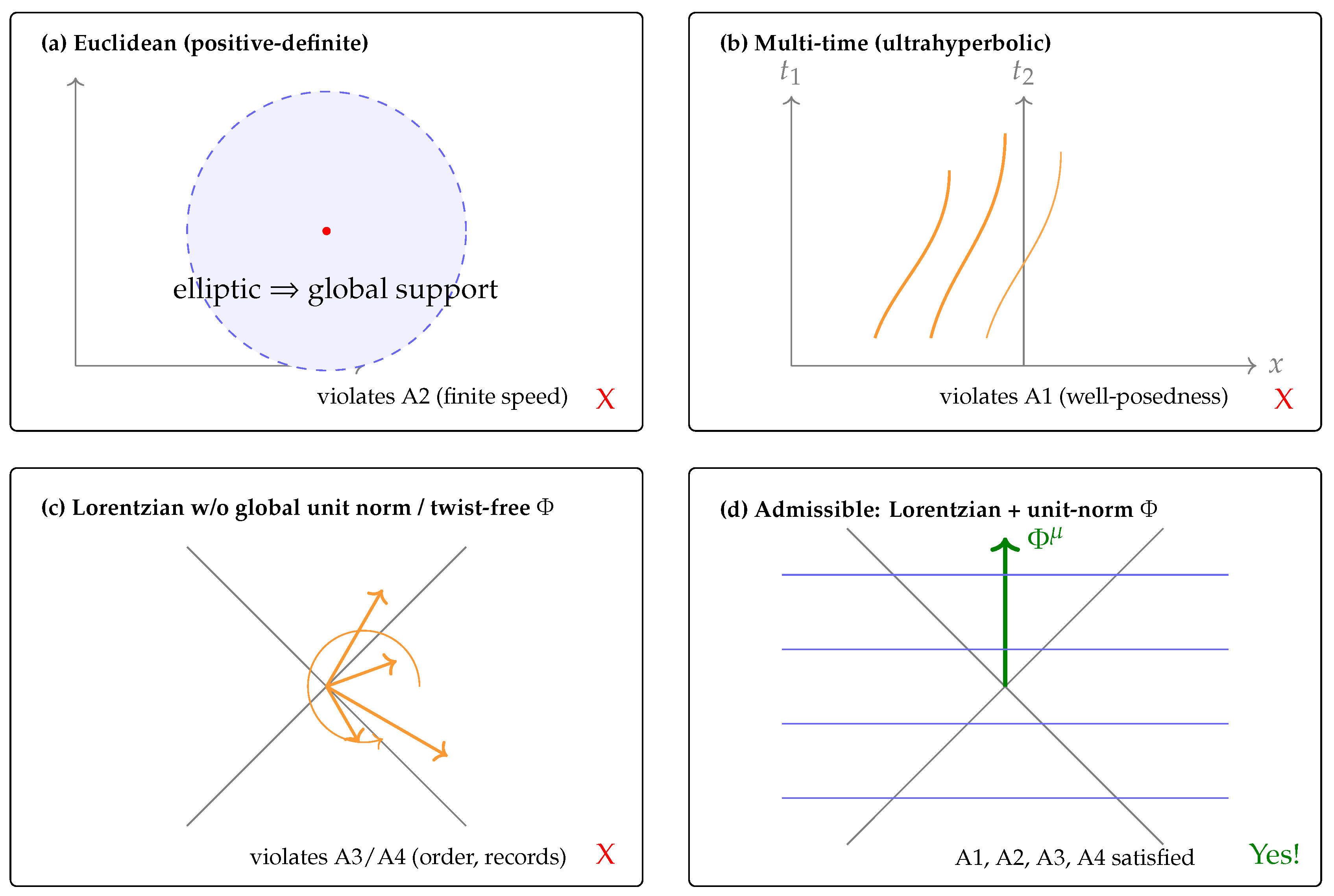
Operational rationale. To clarify that the exclusions in Theorem B are enforced by observer/causality requirements rather than by mere formal preference, we provide short operational justifications in Appendix D. There we show: (i) Euclidean (elliptic) structure yields Green functions with global support, so no sharp domain of dependence exists and finite-speed signalling (A2) fails; (ii) with two or more time directions the equation becomes ultrahyperbolic, the Cauchy problem is ill-posed (exponentially growing high-frequency modes), violating well-posed local dynamics (A1); and (iii) in Lorentzian backgrounds lacking a smooth, future-directed, unit-norm, twist-free , no global time function or foliation is available, undermining acyclic causal order and stable records (A3–A4).
5. Measurement as Selector of the Lorentzian, Unit–Norm Phase
Overview
Theorems 4 and 5 formalize the idea of *measurement as boundary–induced phase selection*. The picture is that a small, initially disordered region is placed next to a large apparatus region that is already aligned in the Lorentzian unit–norm phase. The interface between them acts like a catalyst: the boundary forces to adopt the same phase, erasing disorder and locking in a consistent time direction.
Technical readers should read Appendix C for a rigorous development and proof.
Our approach is based on energy minimization with boundary coupling: a surface term penalizes deviations from the apparatus field . For large coupling , the unique minimizer is shown to align closely with throughout . In addition, the associated gradient flow (a PDE evolution equation) drives any initial configuration toward this aligned state exponentially fast. Finally, large–deviation estimates show that statistical fluctuations away from alignment are exponentially suppressed.
For analogy, one can picture a block of iron touching a magnet: although the block may initially have disordered spins, the boundary interaction with the magnet causes all internal spins to align. In this analogy, plays the role of the magnetized apparatus, and is the region being “measured.”
In systems governed by coarse–grained vector fields with a potential favoring unit–norm, timelike alignment, a measurement-like process can be modeled as a boundary-induced phase transition. Specifically, a disordered microscopic domain becomes embedded within a larger region already stabilized in the Lorentzian, unit–norm phase. This interface interaction drives the interior toward alignment via variational and dynamical principles.
Mathematically, we formulate this as a coupled system on a domain adjacent to a stabilized apparatus region , with boundary . The interaction is described by an interface coupling functional and gradient flow evolution, drawing on tools from PDE theory [22,40] and statistical interface phenomena [11,42].
Setting
Let be a mesoscopic domain initially lacking a coherent time direction, and let be a neighboring region in which a smooth, future–directed, unit–norm, twist–free field is defined on a percolating domain (as established by Theorem 1). We consider the variational functional:
where controls the strength of the interface coupling and is the induced metric on .
Definition 3
(Phase selection via boundary alignment). Given fixed parameters with , phase selection of by occurs if the unique global minimizer of satisfies:
for some as , and the gradient flow converges exponentially to in [51].
Static selection: variational lock-in
Theorem 4
(Boundary–induced alignment). Assume and (ordered phase), and let be smooth, unit–norm, future–directed, and twist–free on . Then there exist constants and such that for all :
- 1.
- Existence and uniqueness: admits a unique minimizer .
- 2.
- Norm pinning: .
- 3.
- Alignment: ; in particular, the angle between and is uniformly small in Ω.
- 4.
- Twist suppression: If is hypersurface–orthogonal on Γ, and the rest of satisfies compatible boundary conditions, then in Ω.
Any competitor misaligned on a set of positive measure obeys the energy gap bound:
where D is the largest misaligned subdomain and σ the domain wall surface tension.
Proof. A complete proof is given in Appendix C (see Propositions C.C.2–C.C.5 and Lemma C.C.4).
Dynamics: convergence and stability
Consider the –gradient flow of :
Theorem 5
(Exponential convergence to the aligned phase). For as in Theorem 4, any initial condition evolves under (10) to with
for some constants . For initial data drawn from the Gibbs ensemble at inverse temperature β, the misalignment probability obeys
indicating exponential concentration of the stationary distribution near .
Proof. A complete proof is given in Appendix C (see Propositions C.C.7–C.C.10 and Theorem C.C.9).
Interpretation.
Theorems 4 and 5 formalize how a stable, unit–norm, twist–free domain can be imposed via boundary coupling. A sufficiently strong interface interaction with a macroscopic aligned region induces both static and dynamical alignment in a previously unordered domain. This models measurement as a robust, physically grounded boundary–induced phase selection mechanism.
See Figure 3 for a schematic illustration of phase selection.
6. Discussion and Conclusions
This work addresses one of the deepest questions in physics: whether the causal spacetime of our everyday experience — with a definite time orientation, Lorentzian signature, and three–dimensional space evolving in time — can emerge from fundamentally pregeometric degrees of freedom, rather than being imposed from the outset. By constructing and analysing a broad statistical ensemble of microscopic chronon variables, we have demonstrated that such a structure not only can arise but can do so with strictly positive probability under generic, physically reasonable conditions.
Theorem A establishes the existence of large–scale Lorentzian, unit–norm domains in the configuration space of coarse–grained chronon fields, stabilized by finite–range ferromagnetic alignment and strong quartic norm–pinning. Theorem B strengthens this to exclusivity, showing that under general axioms for well–posed, causally consistent local dynamics, no alternative signature or non–unit–norm structure can sustain persistent causal order or information–processing observers. Theorem C then provides a dynamical mechanism — measurement as boundary–driven phase selection — by which such domains can be extended and stabilized through interaction, allowing alignment to percolate across boundaries and propagate the ordered phase.
From a physical perspective, these results jointly supply a thermodynamic foundation for three core features of our observed universe:
- Causal structure: Lorentzian signature and a global time function arise naturally in certain finite–range, isotropic ensembles, without requiring them to be postulated a priori.
- Dimensionality selection: While our proofs apply to spacetimes for , physical and stability arguments favour as the most likely large–scale outcome, with integer dimensions selected by universality under coarse–graining [2,6,14,50]. Stability analyses in quantum gravity approaches [13,41] and spectral–dimension flow results [36,38] further support the emergence of three large spatial dimensions in the infrared limit.
- Measurement dynamics: Observation becomes an emergent, dynamical phenomenon in which phase–aligned regions act as seeds, converting disordered surroundings into the Lorentzian, unit–norm phase.
Relation to other approaches.
Our results are complementary to several lines of research on emergent Lorentzian structure and causal order. While graviton–time approaches posit a direct identification between time and the graviton [25,26], our results obtain the same phenomenology—lightcones, a global time function, and stable records—via phase selection in a chronon ensemble, not via a graviton–time equivalence. Clock–field and Euclidean-to-Lorentzian mechanisms derive an effective Lorentzian metric from a deeper Euclidean theory [23,44]; by contrast, the present model is formulated directly as a stochastic, finite–range interaction on pregeometric variables, and Theorem B furnishes an operational exclusivity statement under observer/causality axioms. Signature–change scenarios in emergent/loop-inspired gravity [9] emphasize phase structure of the effective geometry; our Theorem C likewise casts measurement as a boundary–driven phase selection, providing a concrete mechanism for stabilizing and propagating the ordered Lorentzian phase.
Order-first programs such as Causal Set Theory recover continuum Lorentzian geometry from causal order plus volume [10,53]. In our framework the ordered phase supplies a smooth, future-directed, unit–norm, twist–free field that induces a global time function and foliation, thereby realizing causal order at the coarse–grained level and linking it to a microscopic alignment mechanism. Nonperturbative path-integral approaches (Causal Dynamical Triangulations) exhibit extended, de Sitter–like Lorentzian phases [3]; Group Field Theory condensates similarly realize continuum spacetime as a hydrodynamic phase of non-spatiotemporal quanta [47]. Our chronon ensemble offers a statistical–mechanical route in which the same type of phase selection is tied to finite–range alignment and norm pinning, with axiomatic constraints (A1–A4) making explicit why alternative signatures fail. Finally, matrix-model studies (Lorentzian type IIB) show dynamically emergent expanding spacetimes [5,35]; our results can be viewed as a complementary, effective-theory perspective where a macroscopic time vector emerges as an order parameter. Holographic viewpoints that interpret signature as a phase feature tied to entanglement structure [12] are likewise consonant with the phase–selection perspective emphasized here.
The framework developed here is deliberately broad, encompassing a wide class of microscopic Hamiltonians and substrates. This generality suggests several avenues for future work:
- Extending the analysis to non–isotropic couplings and substrates with nontrivial topology, to examine robustness of the Lorentzian phase.
- Exploring quantitative bounds on the percolation rate of phase alignment in more complex geometries.
- Connecting the emergent coarse–grained field to effective Einstein–Hilbert dynamics or other macroscopic gravitational actions.
- Investigating possible observational or experimental signatures of boundary–driven phase propagation in analogue systems.
In conclusion, the results here provide a concrete and mathematically rigorous route from pregeometric degrees of freedom to an emergent spacetime with Lorentzian causal structure, preferred dimensionality, and a built–in mechanism for measurement. This unites questions of causal order, geometry, and observation within a single statistical–mechanical framework, offering a step toward explaining not just the form of the laws of physics, but why the universe presents itself in a way that allows us to exist and to measure it.
Appendix A. Foliation and Proper Time from a Timelike Vector Field
In this appendix we state and prove sufficient conditions under which a smooth, future–directed timelike vector field induces a global time function, a smooth foliation of spacetime into spacelike hypersurfaces orthogonal to , and a corresponding proper–time parameter along its flow. This result underpins the claim that a stabilized chronon field can generate both temporal order and effective Lorentzian geometry at macroscopic scales.
Appendix A.1. Setting and Definitions
- (a)
- is smooth, everywhere timelike, future–directed, and normalized:
- (b)
Appendix A.2. Existence of Orthogonal Hypersurfaces
Theorem A1
Proof.
Define as the –dimensional subspace orthogonal to at each point . Smoothness of implies that is a smooth distribution on . By the Frobenius theorem [27,39], condition (A2) implies that is involutive: if , then .
An involutive, codimension–one distribution integrates to a smooth foliation by hypersurfaces such that . Each hypersurface is spacelike because is timelike and has Lorentzian signature, so is positive–definite. Smoothness of ensures that the foliation depends smoothly on .
Appendix A.3. Proper Time Along Φ μ
Define a scalar function along each integral curve of by
with initial condition on a reference hypersurface . Because is normalized (A1), coincides with the proper time along the flow of [55]:
where is the tangent to the flow.
Introducing adapted coordinates , where are local coordinates on , the vector field takes the form
In these coordinates, the metric splits as
with the induced Riemannian metric on each spacelike hypersurface .
Appendix A.4. Interpretation
This theorem provides a geometric foundation for emergent proper time and spacetime foliation from a single smooth, timelike, unit–norm, twist–free vector field. It implies that any stabilized coarse–grained field satisfying the Frobenius condition gives rise to:
- (i)
- a global (or domain-wide) time function ,
- (ii)
- a smooth foliation by spacelike hypersurfaces orthogonal to ,
- (iii)
- a proper–time parameterization along integral curves of .
Hence, in any macroscopic domain where such a emerges from microscopic dynamics, the basic causal and temporal structures of Lorentzian spacetime—orthogonal foliations, global time coordinates, and metric splitting—are guaranteed to exist without additional assumptions.
Appendix B. Microscopic Model and Coarse–Graining
In this appendix we define the microscopic chronon ensemble, derive the coarse–grained effective action , and state the precise conditions under which Theorem 1 applies. The goal is to exhibit a well–posed statistical–mechanical model whose renormalized large–scale limit yields the ordered–phase –model analyzed in Section 3.
Appendix B.1. Microscopic Chronon Configuration Space
Let be a discrete set of chronon sitesp with bounded density , embedded in a smooth –dimensional manifold M. To each site , assign a microscopic chronon vector, where indexes internal proto–spacetime components. The configuration space is
with Gibbs measure
at inverse temperature , and Hamiltonian
Here:
- are ferromagnetic couplings with finite interaction range .
- is the local potential, with and U smooth, bounded below, and growing at most polynomially.
- The Lorentzian inner product is defined with respect to .
The quartic term pins the Minkowski norm to , selecting unit–norm timelike vectors in the low–temperature limit.
Appendix B.2. Block–Spin Coarse–Graining
Fix a coarse–graining scale , and partition into disjoint blocks of linear size . Each block contains sites. Define the block average
Integrating out intrablock fluctuations yields an effective interblock interaction [28,52]:
with
where are renormalized ferromagnetic couplings at scale , is the renormalized on–site potential, and denotes higher–derivative terms suppressed by or smaller.
Appendix B.3. Continuum Limit and Effective Action
In the limit , the block index i becomes a continuous point , and the discrete Laplacian yields a kinetic term . The effective potential retains its quartic minimum at due to the stability of ordered ferromagnetic phases under renormalization [28,52]. The resulting continuum effective action is
with , in the ordered phase, and ellipsis denoting higher–order or symmetry–breaking terms suppressed at large .
Appendix B.4. Microscopic Conditions for Theorem 1
The assumptions of Theorem 1 are satisfied whenever the microscopic model obeys:
- Finite–range ferromagnetism: for nearest neighbors; for .
- Strong norm–pinning: , ensuring that is the unique deep minimum of V.
- Low–temperature ordering: , where is the critical inverse temperature for long–range order in the corresponding model.
- Isotropy: depends only on ; any Lorentz–violating anisotropies are RG–irrelevant at scale .
Under these conditions, the coarse–grained parameters satisfy , , and , placing the system in the hyperbolic –model universality class , with spontaneous symmetry breaking to a future–directed, unit–norm timelike vector field.
Remark.
This derivation ensures that the effective model inherits all necessary properties for the application of Section 3, including the emergence of Lorentzian signature, unit–norm constraint, and twist–free alignment. The percolation and correlation inequalities used in Theorem 1 then yield the macroscopic Lorentzian, unit–norm phase from first principles.
Appendix C. Rigorous Proof for Theorem C (consequence of Theorem 5.2 and Theorem 5.3)
Throughout, is a smooth, bounded, connected domain with interface to a stabilized apparatus region A. The effective energy is the boundary-coupled functional (cf. (8))
with , , (ordered phase), , and smooth, unit-norm, future-directed, twist-free on A. We work in the Sobolev space , using for the Lorentzian inner product and the standard trace map [1,40].
Appendix C.1. Direct Method, Alignment, Norm Pinning, Uniqueness, Energy Gap
Lemma C.1
(Coercivity up to compact perturbations). There exist constants (depending on ) such that for all ,
Proof.
Proposition C.2
(Existence of a minimizer). For each there exists minimizing on .
Proof.
By Lemma C.1, any minimizing sequence is bounded in . Extract a weakly convergent subsequence in . Weak lower semicontinuity of the convex parts and compactness for the polynomial nonlinearity (plus continuity of the trace) yield [22].
Lemma C.3
(Boundary control ⇒ interior alignment). There exists independent of η such that for any minimizer ,
Proof.
Lemma C.4
(Uniform norm pinning via Modica–Mortola). There exist such that for ,
Proof.
Proposition C.5
(Energy gap for misalignment). There exist (independent of η) such that any competitor misaligned on a set of positive measure satisfies
where D is the largest misaligned subdomain and σ is the domain-wall surface tension.
Proof.
Adapt the Peierls/Ising interface-pinning argument [29] to the present vector model: the boundary term creates a linear (in ) interfacial cost on , while bulk competition across an interface contributes the Allen–Cahn-type surface tension . A standard cut-and-paste comparison with the aligned state yields the inequality.
Appendix C.2. Twist Suppression (ω=0) under Hypersurface-Orthogonal Boundary Data
Assume is simply connected and is hypersurface-orthogonal on (i.e. ), with compatible conditions on (Neumann or Dirichlet). Let denote the twist tensor of .
Lemma C.6
(Curl-free continuation). If the unique minimizer satisfies on Γ (trace sense), then in Ω.
Proof.
The Euler–Lagrange system for is semilinear uniformly elliptic with analytic nonlinearity [30]. Applying the exterior derivative to the 1-form gives a homogeneous, strongly elliptic system for with zero boundary data on and compatible data elsewhere. By unique continuation (or energy methods plus Poincaré on simply connected ), . See also Frobenius integrability in the Lorentzian setting [45].
Appendix C.3. Gradient-Flow Well-Posedness and Exponential Convergence
We now introduce the –gradient flow of the energy (A12), with boundary condition inherited from the interface term:
Proposition C.7
(Global well-posedness & Lyapunov decrease). For any there exists a unique global solution
to (A13), and is non-increasing with
Proof.
with Robin/Neumann boundary is sectorial on ; see semigroup theory [48]. The nonlinearity is locally Lipschitz and subcritical. Semigroup methods give local existence/uniqueness; the Lyapunov identity follows by multiplying (A13) by and integrating by parts. Boundedness of along trajectories prevents blow-up, yielding global existence. □
Lemma C.8
Proof.
Theorem C.9
(Exponential convergence). There exist constants (independent of in a neighborhood of ) such that the solution of (A13) satisfies
Proof.
Linearize (A13) near and use the spectral gap from Lemma C.8 to obtain exponential decay of the linearized dynamics; a standard stability/variation-of-constants argument closes the nonlinear estimates. Alternatively, the Łojasiewicz–Simon gradient inequality [51] for analytic energies yields the same rate since is a nondegenerate critical point.
Proposition C.10
(Large-deviation tail for misalignment). If is sampled from the Gibbs measure at inverse temperature β, then for any ,
for some independent of η.
Proof.
Combine the energy gap of Proposition C.5 with standard large-deviation estimates for Gibbs measures [19].
Appendix C.4. Summary of Conclusions
- Static selection (Theorem 5.2): existence and, for large , uniqueness of the minimizer ; uniform norm pinning ; alignment ; twist suppression under the stated boundary hypotheses; and an energy gap penalizing misalignment on .
- Dynamics (Theorem 5.3): global well-posedness of the gradient flow (A13); a spectral gap at ; exponential convergence ; and a large-deviation tail for misaligned initial data sampled from the Gibbs ensemble.
Appendix D. Operational Rationale for Theorem B (Three “Whys”)
Theorem B (Exclusivity) rests on four operational axioms:
- A1.
- Well-posed local dynamics: the Cauchy problem admits existence, uniqueness, and continuous dependence on initial data on suitable hypersurfaces.
- A2.
- Finite-speed signalling: disturbances propagate inside a sharp domain of dependence (a cone bounded by some speed c).
- A3.
- Acyclic causal order: no closed causal curves (no cycles in the reachability relation).
- A4.
- Stable records: “memory states” can be placed on achronal slices and compared consistently under evolution.
Below we justify why (i) Euclidean (elliptic) structure violates A2, (ii) multi-time (ultrahyperbolic) structure violates A1, and (iii) Lorentzian backgrounds without a global unit–timelike, twist-free violate A3/A4.
Appendix D.1. Why Global Support Violates Finite Speed (A2)
For an evolution equation with (retarded) fundamental solution , finite-speed propagation is equivalent to
so that convolution with a localized source cannot influence points outside the cone.
Hyperbolic benchmark.
In dimensions, the wave equation has
whose support lies on the light cone ; hence (A14) holds with .
Parabolic/elliptic contrast.
For the heat equation,
we have for allx, every . Any localized perturbation instantly produces a nonzero response everywhere (no cone), so A2 fails.
For elliptic problems (Euclidean signature), e.g. Poisson,
the Green function is nonzero for all . There is no time evolution and no domain of dependence; changing data/boundaries alters the solution globally. This global support is the negation of finite-speed propagation, so A2 is violated.
Appendix D.2. Why Multiple Time Directions Cause Divergence (A1)
Let the signature be with time-like directions. The model equation is
Choose as “evolution” time and Fourier transform in :
Equation (A18) becomes the ODE
Whenever , the RHS is with , yielding
High frequencies in the extra times () make arbitrarily large, so arbitrarily small perturbations in the data produce arbitrarily large solutions immediately. No uniform energy estimate or continuous dependence is possible: the Cauchy problem is ill-posed in the sense of Hadamard. Hence A1 fails for multi-time (ultrahyperbolic) backgrounds.
Energy viewpoint.
With , the natural quadratic form is indefinite in the “time” sector, preventing a positive-definite conserved energy; extra time directions allow exponential growth of modes, again contradicting well-posedness.
Appendix D.3. Why Lorentzian without Global Unit–Norm, Twist-Free Φ Violates Order/Records (A3/A4)
A sufficient (and, in standard causality theory, essentially equivalent) condition for stable causality is the existence of a continuous time function strictly increasing along every future-directed causal curve, with timelike gradient . In our framework, a smooth, future-directed field with
guarantees such a by Frobenius: there exists and with
Unit norm pins to proper time along the integral curves of .
Consequences when (A21) holds.
- Acyclic order (A3): If increases strictly along causal curves, a closed causal loop would force and simultaneously—impossible. Hence no cycles.
- Stable records (A4): Records written on achronal leaves can be compared consistently; updates from to are path-independent because globally orders events.
What fails without (A21).
- Nonzero twist (no integrable orthogonal distribution). The –orthogonal planes do not integrate to global hypersurfaces; there is no global with . Operationally this is non-synchronizability (Sagnac-type gaps): transporting clocks around loops yields mismatched times. Without a global time function, standard proofs excluding cycles break down and path-dependent synchronization undermines consistent record comparison. Thus A3/A4 can fail.
- Not globally unit–timelike. If becomes null/spacelike or vanishes somewhere, it cannot serve as an everywhere monotone clock; foliations can break or change causal character. Even if twist vanishes locally, loss of unit timelikeness introduces a rescaling ambiguity for “clock speed”, defeating a global, invariant ordering and the invariance of “write-once” records across the foliation. Again A3/A4 are jeopardized.
Summary.
The combination Lorentzian metric + smooth, future-directed, unit–norm, twist-free Φ provides (i) a lightcone structure (A2), (ii) a well-posed evolution on (A1, under standard regularity), and (iii) a global time function ensuring acyclic order and stable records (A3/A4). Removing any of these ingredients breaks one of the axioms, which is the content of Theorem B.
References
- R. A. Adams and J. F. Fournier, Sobolev Spaces, 2nd ed., Academic Press, 2003.
- J. Ambjørn, J. Jurkiewicz, and R. Loll, “Reconstructing the Universe,” Phys. Rev. D 72, 064014 (2005). [CrossRef]
- J. Ambjørn and R. Loll, “Causal Dynamical Triangulations,” arXiv:2401.09399 [hep-th] (2024).
- J. Ambjørn and R. Loll, “Causal Dynamical Triangulations: Gateway to Nonperturbative Quantum Gravity,” arXiv:2401.09399 [hep-th] (2024).
- Y. Asano, T. Aoyama, H. Kawai, and Y. Yoshida, “Defining the Type IIB Matrix Model without Breaking Lorentz Symmetry,” Phys. Rev. Lett. 134, 041603 (2025). [CrossRef]
- B. Bahr, S. Steinhaus, “Investigation of the Spinfoam Path Integral with Quantum Cuboids,” Phys. Rev. D 93, 104029 (2016). [CrossRef]
- C. Bär, N. Ginoux, and F. Pfäffle, Wave Equations on Lorentzian Manifolds and Quantization, EMS, 2007.
- A. N. Bernal and M. Sánchez, “On Smooth Cauchy Hypersurfaces and Geroch’s Splitting Theorem,” Commun. Math. Phys., vol. 243, pp. 461–470, 2003. [CrossRef]
- M. Bojowald, E. I. Duque, and D. Hartmann, “A new type of large-scale signature change in emergent modified gravity,” Phys. Rev. D 109, 084001 (2024). [CrossRef]
- M. Braun, “Spacetime reconstruction by order and number,” arXiv:2507.01907 [gr-qc] (2025). [CrossRef]
- H. Brezis, Analyse Fonctionnelle, Dunod, 1998.
- M. B. Cantcheff, “Signature change as phase transition in holography,” arXiv:2505.13349 [hep-th] (2025). [CrossRef]
- S. Carlip, “Spontaneous Dimensional Reduction in Short-Distance Quantum Gravity?,” AIP Conf. Proc. 1196, 72 (2009).
- S. M. Carroll, Spacetime and Geometry: An Introduction to General Relativity, Cambridge University Press, 2019.
- Y. Choquet-Bruhat, General Relativity and the Einstein Equations, Oxford Univ. Press, 2009.
- R. Courant and D. Hilbert, Methods of Mathematical Physics, Vol. II, Wiley, 1962.
- W. Craig, T. Kappeler, and W. Strauss, “Microlocal Dispersive Smoothing for the Schrödinger Equation,” Commun. Pure Appl. Math., vol. 63, pp. 597–629, 2009. [CrossRef]
- E. De Giorgi, “Sulla differenziabilità e l’analiticità delle estremali degli integrali multipli regolari,” Mem. Accad. Sci. Torino Cl. Sci. Fis. Mat. Nat. (3) 3 (1957), 25–43.
- A. Dembo and O. Zeitouni, Large Deviations Techniques and Applications, 2nd ed., Springer, 1998.
- P. A. M. Dirac, Lectures on Quantum Mechanics, Yeshiva Univ., 1964.
- R. S. Ellis, Entropy, Large Deviations, and Statistical Mechanics, Springer, 1985.
- L. C. Evans, Partial Differential Equations, 2nd ed., AMS, 2010.
- J. C. Feng, S. Mukohyama, and S. Carloni, “Emergent Lorentzian dispersion relations from a Euclidean scalar–tensor theory,” arXiv:2505.00112 [gr-qc] (2025). [CrossRef]
- C. M. Fortuin, P. W. Kasteleyn, and J. Ginibre, “Correlation Inequalities on Some Partially Ordered Sets,” Commun. Math. Phys., vol. 22, pp. 89–103, 1971.
- O. Flomenbom, “The Gravity Field: In the Origin of Matter and Almost Everywhere Else,” Reports in Advances of Physical Sciences 08, 2450003 (2024). [CrossRef]
- O. Flomenbom, “The Imaginary Mass Field: In all Known Forces,” Reports in Advances of Physical Sciences (2025).Functional Analysis, Sobolev Spaces and Partial Differential Equations, Springer, 2011 . [CrossRef]
- G. Frobenius, “Über das Pfaffsche Problem,” J. Reine Angew. Math. 82, 230–315 (1877).
- J. Fröhlich and T. Spencer, “The Kosterlitz–Thouless Transition in Two–Dimensional Abelian Spin Systems and the Coulomb Gas,” Commun. Math. Phys., vol. 81, pp. 527–602, 1981.
- G. Gallavotti, Statistical Mechanics: A Short Treatise, Springer, 1999.
- D. Gilbarg and N. S. Trudinger, Elliptic Partial Differential Equations of Second Order, Springer, 2001.
- R. B. Griffiths, “Correlations in Ising Ferromagnets. I,” J. Math. Phys., vol. 8, pp. 478–483, 1967. [CrossRef]
- G. Grimmett, Percolation, 2nd ed., Springer, 1999.
- J. Hadamard, Lectures on Cauchy’s Problem in Linear Partial Differential Equations, Yale Univ. Press, 1923.
- S. W. Hawking and G. F. R. Ellis, The Large Scale Structure of Space-Time, Cambridge Univ. Press, 1973.
- M. Hirasawa, K. N. Anagnostopoulos, T. Azuma, K. Hatakeyama, J. Nishimura, S. Papadoudis, and A. Tsuchiya, “The emergence of expanding space-time in the Lorentzian type IIB matrix model with a novel regularization,” arXiv:2307.01681 [hep-th] (2023). [CrossRef]
- P. Hořava, “Quantum Gravity at a Lifshitz Point,” Phys. Rev. D 79, 084008 (2009). [CrossRef]
- L. P. Kadanoff, “Scaling Laws for Ising Models Near Tc,” Physics, vol. 2, pp. 263–272, 1966. [CrossRef]
- O. Lauscher and M. Reuter, “Fractal Spacetime Structure in Asymptotically Safe Gravity,” JHEP 10, 050 (2005).
- J. M. Lee, Introduction to Smooth Manifolds, 2nd ed., Springer, 2013.
- J. L. Lions and E. Magenes, Non-Homogeneous Boundary Value Problems and Applications, Springer, 1972.
- R. Loll, “Quantum Gravity from Causal Dynamical Triangulations: A Review,” Class. Quantum Grav. 37, 013002 (2020). [CrossRef]
- L. Modica and S. Mortola, “Un esempio di Γ-convergenza,” Boll. UMI, 14-B, 285–299, 1977.
- J. Moser, “A new proof of De Giorgi’s theorem concerning the regularity problem for elliptic differential equations,” Comm. Pure Appl. Math. 13 (1961), 457–468. [CrossRef]
- S. Mukohyama and J.-P. Uzan, “From configuration to dynamics: Emergence of Lorentz signature in classical field theory,” Phys. Rev. D 87, 065020 (2013). ::contentReference[oaicite:8]index=8. [CrossRef]
- B. O’Neill, Semi-Riemannian Geometry, Academic Press, 1983.
- E. Olivieri and M. E. Vares, Large Deviations and Metastability, Cambridge Univ. Press, 2005.
- D. Oriti, “Tensorial Group Field Theory condensate cosmology as an example of spacetime emergence in quantum gravity,” arXiv:2112.02585 [gr-qc] (2021).
- A. Pazy, Semigroups of Linear Operators and Applications to Partial Differential Equations, Springer, 1983.
- H. Ringström, The Cauchy Problem in General Relativity, European Mathematical Society, 2009.
- M. Reuter and F. Saueressig, “Quantum Einstein Gravity,” New J. Phys. 14, 055022 (2012). [CrossRef]
- L. Simon, “Asymptotics for a class of nonlinear evolution equations,” Ann. Math., vol. 118, pp. 525–571, 1983. [CrossRef]
- B. Simon, The Statistical Mechanics of Lattice Gases, Vol. I, Princeton University Press, 1993.
- S. Surya, “The causal set approach to quantum gravity,” Living Rev. Relativity 22, 5 (2019). [CrossRef]
- M. E. Taylor, Partial Differential Equations I: Basic Theory, 2nd ed., Springer, 2011.
- R. M. Wald, General Relativity, University of Chicago Press, 1984.
- N. M. J. Woodhouse, Geometric Quantization, Oxford Univ. Press, 1992.
- M. Zahradník, “An alternate version of Pirogov–Sinai theory,” Commun. Math. Phys., vol. 93, pp. 559–581, 1984.
- J. Zinn-Justin, Quantum Field Theory and Critical Phenomena, 4th ed., Oxford University Press, 2002.
Figure 1.
Schematic of emergence and selection. (a) Microscopic chronon vectors are disordered. (b) Block–spin coarse–graining yields an effective field with stiffness and norm pinning. (c) A stabilized apparatus region aligns the microscopic domain across the interface , driving it into the Lorentzian, unit–norm phase; the alignment front can propagate into progressively larger regions.
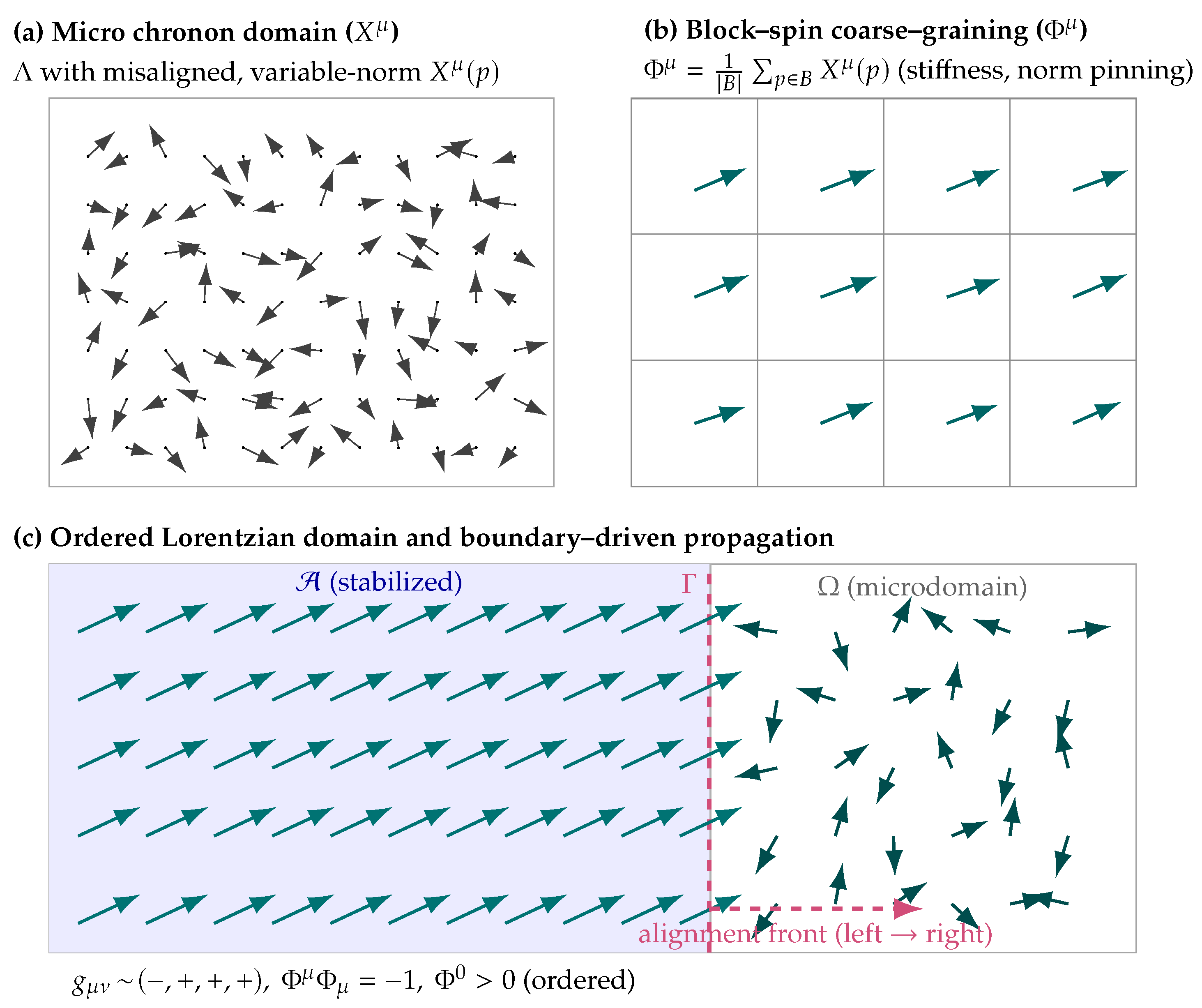
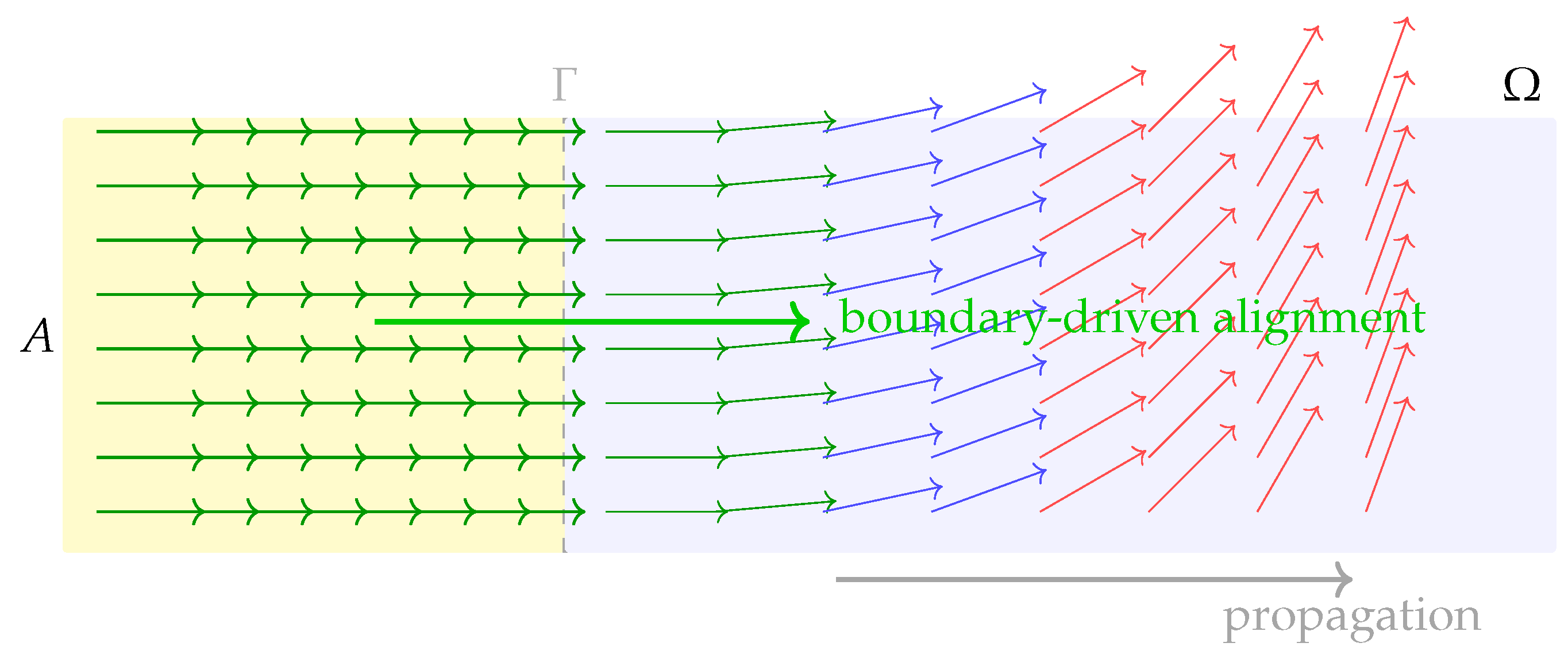
Figure 3.
Measurement as boundary–driven phase selection. The left region is a stabilized apparatus A (yellow), the right region is the system (blue). The dashed line marks the interface . In A, arrows represent an aligned, unit–norm, twist–free field (ordered Lorentzian phase). Coupling across (thick green arrow) enforces alignment at the boundary and seeds an alignment front into : near (green arrows) the field is aligned; farther to the right the orientation gradually deviates (blue → red arrows). This illustrates the boundary functional selecting the ordered phase in : for sufficiently large interface strength , the unique minimizer aligns with A, pins the norm (), suppresses twist (), and the associated gradient flow drives exponential convergence to the aligned phase. Because the boundary bias percolates, the ordered domain expands into , providing a dynamical, measurement–like mechanism for phase selection and stabilization.
Disclaimer/Publisher’s Note: The statements, opinions and data contained in all publications are solely those of the individual author(s) and contributor(s) and not of MDPI and/or the editor(s). MDPI and/or the editor(s) disclaim responsibility for any injury to people or property resulting from any ideas, methods, instructions or products referred to in the content. |
© 2025 by the authors. Licensee MDPI, Basel, Switzerland. This article is an open access article distributed under the terms and conditions of the Creative Commons Attribution (CC BY) license (http://creativecommons.org/licenses/by/4.0/).
Copyright: This open access article is published under a Creative Commons CC BY 4.0 license, which permit the free download, distribution, and reuse, provided that the author and preprint are cited in any reuse.


