Submitted:
26 August 2025
Posted:
27 August 2025
You are already at the latest version
Abstract
We present Chronon Field Theory (CFT), a covariant framework in which large–scale spacetime geometry—including temporal order and causal structure—emerges from the coarse–grained dynamics of a single future–directed timelike field Φμ(x). Within this approach, both the unit–norm property of Φμ and the Lorentzian signature of gμν are not postulated but arise uniquely from random microscopic chronon dynamics under broad symmetry and locality assumptions. Quantum phenomena are reinterpreted in this geometric setting: double–slit interference results from phase–coherent Φ–threads rather than superposed particle paths, and measurement appears as a boundary–induced alignment of microscopic orientations with the apparatus’s macroscopic field, yielding definite outcomes without collapse or branching. Schrödinger’s cat is then a straightforward macro–micro coupling with no persistent macroscopic superposition, while EPR–type entanglement reflects shared Φ–thread ancestry across spacelike separations. The Born rule follows from the unbiased martingale structure of alignment dynamics and from coarse–graining symmetries, making it an emergent statistical law; the uncertainty principle appears as a statistical bound on chronon fluctuations, with ℏ arising as the variance of coarse–grained action. CFT thus provides a covariant and ontologically economical framework linking spacetime symmetries to quantum measurement, and predicts scale–dependent effects—such as nonlinear decoherence and curvature–sensitive timing shifts—that are open to experimental test.
Keywords:
quantum measurement
; decoherence and classicality
; causal structure
; chronon field theory
; quantum gravity foundations
; problem of time
; relational quantum mechanics
; general boundary formulation
; scale-dependent geometry
; path integrals over causal structures
; boundary-induced alignment
; foundations of quantum mechanics
; Born rule
; double-slit experiment
; entanglement
; Schrödinger’s cat
; quantum paradoxes
; uncertainty principle
1. Introduction
Quantum theory remains unmatched in predictive success, yet its conceptual foundations continue to raise long–standing tensions [13,72]. Puzzles and paradoxes persist—the measurement problem [103,112], wave–particle duality [18,36], Schrödinger’s cat [93], and the nonlocal correlations revealed by Bell’s theorem [12]. Each of these signals a mismatch between the quantum formalism and the background spacetime structure inherited from classical physics.
The measurement problem remains the most prominent example. In standard quantum mechanics, states evolve unitarily under the Schrödinger equation, yet measurements yield single, definite outcomes. Copenhagen–type accounts [18,57] introduce a collapse tied to a classical observer, but without a well-defined quantum–classical boundary. The Many–Worlds Interpretation [34,106] preserves unitarity at the price of postulating a vast multiplicity of parallel worlds, but still can’t recover the Born rule without circularity [91]. Decoherence–based accounts [92,115] explain interference suppression in practice, but can’t explain why a single result is experienced.
Wave–particle duality presents a familiar difficulty. In the double–slit experiment, an undisturbed particle yields an interference pattern, while path detection eliminates the fringes and leaves localized impacts [36]. Conventional accounts explain this by invoking either nonlocal collapse or the proliferation of branches, but neither option integrates well with a relativistic and ontologically economical framework.
This paper develops Chronon Field Theory (CFT), a covariant geometric framework designed to reframe these foundational problems. CFT begins with a microscopic timelike field , whose coarse–graining across many fine–grained regions produces a smooth, future–directed macroscopic field , the chronon field. Recent results show that both the Lorentzian signature of and the unit–norm property arise dynamically and uniquely from a broad class of microscopic chronon models (Appendix A, Ref. [69]). In the same spirit, the Born rule is no longer an assumed axiom but follows from CFT’s intrinsic locality, symmetry, and coarse–graining structure (Appendix L, Ref. [70]).
Alignment Structure in CFT
A central organising principle of CFT is the distinction between microscopic and macroscopic alignment:
- Fine–grained quantum regions: Each small spacetime region in the quantum regime has a well–defined local timelike , but orientations are generally uncorrelated between regions.
- Potential average alignment: Within a given region, microscopic fluctuations exhibit a statistical bias toward some local direction.
- Macroscopic correlation: In a stable apparatus, many regions share a robust global alignment that defines the apparatus’s causal geometry.
- Measurement as alignment locking: During measurement, the potential average directions of a microscopic system become aligned with the apparatus’s , producing a definite outcome without nonlocal collapse or many–world branching.
- Uncertainty from statistical geometry: The quantum uncertainty principle arises as a statistical constraint on chronon fluctuation coherence, with the Planck constant ℏ emerging dynamically as the variance of action across coarse-grained chronon ensembles.
Within this framework, Schrödinger’s cat is a straightforward macro–micro coupling: the cat’s macroscopic is already aligned long before the trigger event, so no long–lived macroscopic superposition exists. Entanglement is reinterpreted as two subsystems sharing a –thread ancestry, so that measurement in one domain constrains correlations in the other without superluminal influence. The double–slit experiment is explained similarly: multiple –thread configurations can coexist within a small coherence domain, sustaining interference; path detection couples one thread to a macro–coherent domain, breaking cross–thread phase coherence.
Scope and Status of the Present Work
With Appendices A and T addressing the emergence of spacetime structure and the Born rule, CFT now offers a covariant, ontologically economical framework in which both features are derived from underlying dynamics. In the main text, we present qualitative, conceptual accounts of three central quantum phenomena: the measurement problem (Section 4), the double–slit experiment (Section 5), and entanglement (Section 6.2). For each, the corresponding mathematical formulation and rigorous derivations are deferred to dedicated appendices: Appendix E (measurement problem), Appendix J (double slit), and Appendix K (entanglement). This separation allows the main text to remain accessible while providing full technical detail for specialists.
Open directions include the formulation of a fully general action principle and a complete quantisation of and . The theory yields scale–dependent predictions such as nonlinear decoherence and curvature–sensitive timing shifts, offering concrete opportunities for experimental test.
The paper is organised as follows. Section 2 situates CFT within the wider interpretative landscape. Section 4 develops the account of measurement as geometric embedding. Section 5 treats the double–slit experiment. Section 6.1 and Section 6.2 discuss Schrödinger’s cat and entanglement. Section 10 presents potential empirical probes. Section 12 summarises and compares CFT with Copenhagen, Many–Worlds, and QBist/Relational approaches.
2. Theoretical Context
Chronon Field Theory (CFT) grows out of a long–standing tension between the roles of time and geometry in quantum theory and in relativity. In textbook quantum mechanics, time is an external parameter—a background clock carried over from classical mechanics. In general relativity, it is one coordinate in a dynamical spacetime. Bridging this gap has driven decades of work on quantum gravity and related formalisms [60,65].
CFT, as developed here, is not yet a full theory from first principles. It is a covariant geometric framework that replaces both the background notion of time and the assumption of a fixed spacetime geometry with a single dynamical causal field. Within this picture, quantum phenomena such as interference and measurement arise from interactions between regions whose fine–grained alignment properties differ—particularly between domains in which local chronon orientations are only statistically biased toward a direction, and those in which such biases are strongly correlated over macroscopic scales.
2.1. Time, Geometry, and Causality as Scale–Dependent
In the standard formulation, time lies outside the Hilbert space and remains fixed, while space and time are treated asymmetrically. That description falters in regimes without a global time coordinate—early–universe cosmology, black hole interiors, and other strongly curved settings.
Relational–time approaches [86] and internal–clock models [80] recover time from correlations between variables, but still assume a fixed Lorentzian background. CFT goes further: both causal order and smooth geometry emerge from a dynamical timelike field whose microscopic behaviour is disordered. At Planck scales fluctuates strongly and no stable causal structure exists. At quantum scales, any fine–grained region—whether in empty space or inside a detector—is never perfectly aligned; instead, it exhibits a potential average alignment direction obtained via coarse–graining. In stable macroscopic systems, these local potential averages are highly correlated, producing a globally aligned, future–directed, unit–norm field that defines a local arrow of time and the emergent Lorentzian metric. Between these extremes lie regimes with partial causal–geometric coherence, in which multiple alignment domains can coexist.
2.2. Measurement Without Collapse or Branching
The standard measurement problem—how definite outcomes arise—remains unresolved. Collapse models [10,46] introduce stochastic terms at the cost of Lorentz covariance. Many–Worlds [34,106] keeps unitarity but multiplies ontology. Relational and epistemic views [40,87] economise on ontology but risk reducing the quantum state to bookkeeping.
CFT stays single–world and observer–independent [42,63]. A measurement is the alignment–locking of a microscopic domain’s potential average chronon orientation to the global alignment of a macroscopic apparatus. Before interaction, each fine–grained region of the microscopic system has only a statistical bias toward a direction; after interaction, those biases become correlated with the apparatus’s already coherent . The apparatus does not impose a perfect microscopic order, but rather synchronises the existing statistical tendencies so that subsequent evolution is referenced to its stable geometry. What appears as “collapse” is, in this view, a boundary–induced stabilisation of alignment and local geometry (Appendix E).
2.3. Relation to Geometric Approaches
Quantum theory has long been framed in geometric terms—the projective Hilbert space with its Fubini–Study metric [6,64], Berry’s phase [14], symplectic and contact structures [21]. Quantum–gravity programs—causal sets [17], loop quantum gravity [88], spin foams [81]—build spacetime from discrete or algebraic data and give causal order a primary role.
CFT shares the focus on causal geometry but takes the generator to be a smooth, dynamical timelike vector field producing both intrinsic time and the macroscopic metric. When is globally uniform, standard quantum mechanics in a fixed background is recovered. When it varies, domains can exist in which causal and geometric structure are only partially formed and the fine–grained chronon orientations remain statistically disordered.
2.4. Place in the Landscape
The chronon field unifies three strands of foundational work:
- Relational, dynamical time–geometry: absolute time and fixed metric are replaced by a field–driven, scale–dependent causal structure that can fluctuate or fail at small scales.
- Covariant geometric formulation: the framework is background–independent, Lorentz–compatible, and naturally extendable toward quantum–gravity regimes.
- Minimal ontology with dynamical outcome selection: definite results emerge from bias–lock stabilization without branching worlds or ad hoc collapse rules.
With spacetime causal structure and the Born rule derivable from chronon dynamics, CFT has moved beyond a purely heuristic template toward a coherent, testable framework. Open directions include deriving ’s dynamics from a fully general action principle, quantising and , and characterising departures from perfect causal–geometric coherence. Such deviations could yield observable signatures in high–precision interferometry, relativistic quantum information protocols, and potentially in quantum–gravity–scale experiments.
3. Chronon Field Theory: Core Framework
Chronon Field Theory (CFT) is a covariant, background–independent reformulation of quantum mechanics in which the effective spacetime geometry—both its temporal structure and causal order—emerges, at sufficiently coarse–grained scales, from a smooth, future–directed, unit–norm timelike vector field [73,104]. This chronon field replaces the role of external time in conventional formulations, while also generating the Lorentzian metric structure in which events are embedded. In this view, the familiar large–scale geometry of spacetime is not presupposed at the microscopic level, but appears as an ordered phase of the chronon field.
Recent rigorous results (Appendix A, Ref. [69]) show that both the Lorentzian signature of and the unit–norm property arise dynamically and uniquely from a broad class of microscopic chronon dynamics, replacing earlier postulates. At sub–Planckian or quantum scales, the underlying causal field can fluctuate strongly, with norms and directions varying significantly between regions. In such fine–grained domains, no perfect alignment exists; instead, each exhibits only a statistical bias or potential average toward a local time direction. The smooth of CFT is thus an emergent, coarse–grained descriptor encoding the correlated average alignment of many microscopic regions. In a macroscopic apparatus, these local biases are strongly correlated, yielding a robust global ; in a microscopic quantum system, correlations are weaker and the average alignment less stable.
3.1. The Effective Chronon Field
We consider a smooth, future–directed vector field satisfying
throughout the coarse–grained domain of validity. The integral curves of —chronon threads—define the intrinsic time direction and generate proper–time evolution. The metric appearing here is the large–scale geometry compatible with and, in CFT, emerges alongside it from microscopic dynamics (Appendix A).
For a rigorous statement of the conditions under which such a yields a global time function, spacelike foliation, and proper time, see Appendix A.
3.2. Emergent Temporal and Geometric Foliation
Given a sufficiently smooth , one can define a family of spacelike hypersurfaces orthogonal to , labelled by a scalar function interpreted as intrinsic proper time. In CFT, these hypersurfaces are part of the emergent geometry generated by the large–scale ordering of itself, not embedded in a pre–existing background.
When is hypersurface–orthogonal, the twist tensor vanishes [38]:
where projects orthogonally to .
In that case, satisfies:
with lapse function:
The then act as intrinsic time–slices for quantum evolution. A proof that such a foliation and proper–time structure emerge under the stated regularity and integrability conditions is given in Appendix A. In regions where loses coherence—because the microscopic fluctuations fail to yield a stable average—the foliation and effective metric may break down.
3.3. Action Principle and Dynamical Foundations
While the preceding discussion treats and its induced geometry at the effective, coarse–grained level, a natural next step is to formulate CFT within a fully covariant variational framework. Appendix B presents a candidate general action principle in which the chronon field couples to curvature and gauge sectors via geometric invariants built from , , and their derivatives. In this construction, the unit–norm property of is enforced dynamically through a Lagrange multiplier, while the gravitational and gauge dynamics arise from curvature terms and covariant field strengths projected along and orthogonal to .
The purpose of this appendix is not to claim a definitive microscopic completion, but to provide a coherent starting point from which both classical and quantum equations of motion can be derived, and to clarify how known field theories may emerge as special limits of the chronon–field dynamics.
3.4. Quantum Dynamics Along Causal Threads
In CFT, quantum evolution proceeds in intrinsic proper time along ’s integral curves, rather than in an external coordinate time. Each carries a Hilbert space , and we postulate an evolution law:
where depends on the matter content and the –induced geometry.
In the ADM (3+1) decomposition [3], is expressed via the unit normal to and a shift :
In synchronous gauge (), the Hamiltonian takes the form:
A full derivation from a CFT–specific microscopic action remains for future work.
3.5. Relational Status of the Hilbert Space
As shown in Appendix C, is defined relationally—with respect to the foliation and metric structure induced by —and may fail to exist in regions where loses coherence. This is a departure from the global, time–independent Hilbert space of standard QM. Features include:
- Local definition tied to the domain of coherent and its induced geometry.
- Adaptation to dynamically evolving causal and metric structure.
- Interpretation as a correlation space, not a primitive, background object.
3.6. Gauge and Constraint Structure
As a covariant theory, CFT enforces first–class constraints:
including Gauss, diffeomorphism, and Hamiltonian constraints [59]. Compatibility of a dynamical and its emergent with this algebra is assumed at present; proof of closure is an open technical question.
3.7. Recovery of Standard QM in Smooth Limits
When is constant and spacetime is flat,
coincides with coordinate time t, and the standard Schrödinger equation is recovered:
Thus CFT reduces to conventional QM in the fully coherent, smooth limit—while offering a framework to handle regimes where causal and geometric order are incomplete or scale–dependent.
4. Measurement as Local Geometric Stabilization
In standard quantum theory, a measurement is described either as a sudden “collapse” of the wavefunction [103], or—more recently—as the result of environmental decoherence in a larger Hilbert space [92,115]. CFT takes a different starting point: a measurement is neither an epistemic update nor an external “intervention,” but a local and scale–dependent reconfiguration of causal geometry. It occurs when the average potential alignment direction of a microscopic domain—initially fluctuating and only statistically biased—locks into the global alignment of a macro–coherent apparatus.
At the fine–grained level, no region is perfectly aligned: the microscopic field exhibits fluctuations in both norm and direction. What distinguishes a macro–coherent apparatus from an isolated quantum system is not the absence of fluctuations, but the strong correlation of local potential averages. In a macroscopic device, many small subregions have potential alignment directions that are themselves closely aligned, producing a robust global . In a microscopic quantum system, these correlations are weak; neighbouring subregions can have differing biases, so the coarse–grained average is unstable.
Measurement, in this framework, is the process by which the microscopic domain’s coarse–grained average chronon orientation becomes correlated with—and stabilized by—the apparatus’s global . This is not merely a choice of a time direction, but the embedding of the system’s causal microstructure into the apparatus’s stable spacetime patch. Once this embedding is complete, subsequent evolution proceeds relative to the apparatus’s emergent geometry.
A central result of this account is that, under general locality, symmetry, and coarse–graining conditions natural to CFT, the statistical distribution of possible stabilized outcomes obeys the Born rule. Appendix L (Ref. [70]) summarises the derivation, showing that the rule emerges from the geometric alignment mechanism itself, without being imposed as an independent axiom. Thus, in CFT, both the occurrence of definite outcomes and the quantitative probabilities governing them follow from the same underlying chronon dynamics.
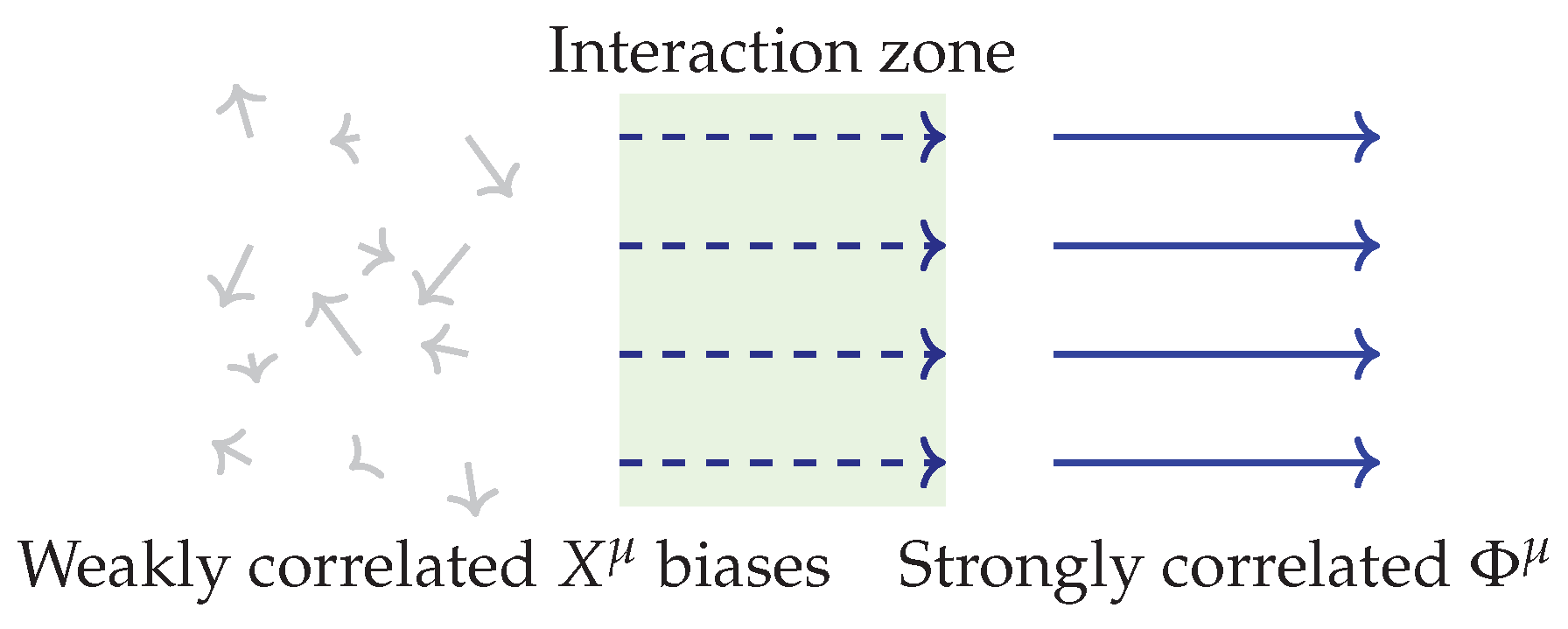
Figure 1.
Measurement as bias correlation: a microdomain with locally fluctuating chronon orientations (left) enters the coarse–graining scale of a macro–coherent apparatus (right). Within the interaction zone, the microdomain’s potential alignment directions become correlated with the apparatus’s global , stabilizing its average time direction and embedding it in the apparatus’s causal geometry.
4.1. Pre-measurement: Locally Biased, Globally Incoherent
Before interaction, the microscopic domain is described by a fluctuating timelike field that does not satisfy the unit–norm constraint and whose preferred directions vary from one fine–grained subregion to another:
The norm and direction vary across the region, producing only short–range correlations and no stable global . The geometry in this regime is statistical and short–lived, resembling a “pre–causal foam” [109]. Quantum indeterminacy here reflects the multiplicity of compatible coarse–grainings of these local biases into different potential alignment directions.
4.2. Scale–Dependent Coupling to the Apparatus
When the microdomain interacts with a macro–coherent apparatus, the effective coarse–graining scale increases. Local biases in first align with their immediate neighbours, then with larger correlated regions, until they are locked to the apparatus’s global . This multi–scale locking process is gradual:
In this picture, what standard QM calls “wavefunction collapse” corresponds to the point at which the correlation extends across the entire microdomain, leaving no room for incompatible alignment histories.
4.3. Hierarchy of Stabilization Scales
The stabilization process can be viewed as a hierarchy of scales:
- Microscopic: fine–grained subregions with fluctuating , weakly biased.
- Mesoscopic: intermediate domains where local averages are partially correlated.
- Macroscopic: global apparatus with strong long–range correlation.
Measurement is complete when correlations have percolated from the microscopic to the macroscopic scale, embedding the system’s causal structure into that of the apparatus.
CFT models the emergence of classicality as a hierarchy:
- Planck scale: maximal disorder; no persistent bias or geometry.
- Quantum scale: weakly correlated local biases; interference possible between regions of different potential alignment.
- Mesoscopic scale: intermediate correlation; some directions stabilized, others fluctuating.
- Macroscopic scale: strongly correlated biases; global stable under perturbations, defining a persistent causal geometry.
Measurement is the embedding of a weakly correlated bias structure into a strongly correlated one, forcing the smaller system into the latter’s global alignment and thereby producing a definite outcome without requiring nonlocal collapse or branching worlds.
5. The Double-Slit Experiment in Chronon Field Theory
The double-slit experiment remains one of the clearest demonstrations of quantum coherence [36]. In conventional accounts, a particle is said to display “wave–particle duality,” with collapse or branching invoked when a which–path detector is present. CFT reframes this entirely in terms of the causal–geometric properties of : interference occurs when the local potential average alignment directions of the chronon field remain sufficiently correlated across both paths at the experiment’s scale, and disappears when those correlations are broken by embedding one path into the macro–coherent domain of a detector. See Figure 2.
5.1. Two Levels of Chronon Correlation
We distinguish between:
- Microscopic (local) correlation: Within a small spacetime region, the fine–grained field fluctuates, but the distribution of its orientations can be biased in such a way that phase relations are maintained across multiple paths. This bias correlation—though far from perfect alignment—is sufficient to sustain interference if preserved over the relevant path separation.
- Macroscopic (global) correlation: Across a large domain, the local potential averages themselves are strongly correlated in direction, yielding a stable, coarse–grained that defines a single time orientation and supports persistent, classical records.
In a detector–free double–slit setup, the “microsystem”—the quantum excitation plus the narrow regions of bias along each path—remains in the first regime. The bias orientations along the two paths remain correlated enough to sustain a shared phase reference, since no macroscopic causal boundary forces them into different alignments.
5.2. Interference as Correlated Bias Histories
The apparent “superposition” is reinterpreted as the joint evolution of bias–correlated –threads—integral curves of the coarse–grained —through both slits inside a single, locally correlated microstructure. Let and be two such bias–carrying threads from the source to a point on the screen. The detection amplitude is modeled heuristically as:
where encodes the stability of the bias correlation along that thread. Interference occurs when both threads retain a mutual phase reference defined by their shared bias correlation.
5.3. Detector Interaction: Bias Lock–in to Macro Alignment
Placing a which–path detector at one slit changes the bias–correlation structure at the experiment’s scale. The detector belongs to a macroscopic apparatus whose is already in the strong–correlation phase. When a microscopic bias–carrying thread encounters this domain, the boundary interaction locks its local potential average orientation to the apparatus’s global .
This locking process destroys the original bias correlation between the two paths: the aligned path now shares the apparatus’s global orientation, while the unmeasured path retains its original local bias. From the coarse–grained viewpoint, the allowed histories reduce to a single bias–compatible thread. Interference disappears—not through nonlocal collapse, but because causal–geometric bias correlations have been severed at the relevant scale, as illustrated in Figure 3.
Remark.
For a mathematical treatment of the double–slit experiment within Chronon Field Theory, including formal definitions of bias–phase coherence, ancestry overlap, and fringe visibility, see Appendix J.
5.4. Summary
In CFT, interference requires only the persistence of correlated local potential averages across both paths—not global unit–norm alignment of . A measurement corresponds to the irreversible coupling of one path’s bias orientation to a macro–coherent domain, fixing its large–scale time orientation and eliminating the shared phase reference needed for interference. This explains how a microsystem can exhibit interference in one configuration yet yield a definite outcome when one path is monitored.
6. Other Foundational Puzzles in CFT
The double–slit experiment shows how CFT replaces the usual “wave–particle” story with a scale–dependent causal–geometric one. Two other famous puzzles—Schrödinger’s cat and quantum entanglement—pose the same conceptual challenge in different limits: (1) the junction between microscopic and macroscopic domains, and (2) correlations maintained across spacelike separation. In CFT, both can be reframed in terms of local bias correlations in the fine–grained chronon field and the persistence of shared causal ancestry.
6.1. Schrödinger’s Cat: Macro–Micro Bias Coupling
In the usual account [93], a microscopic quantum event (e.g. a decay) triggers a macroscopic consequence (a cat’s life or death). Linear quantum evolution then seems to extend the superposition to the cat—something never seen in actual macroscopic systems.
In CFT, the setup contains two domains with very different correlation scales:
- Macroscopic domain (cat, detector, box): strongly correlated local biases; at the coarse–graining scale of the apparatus, the emergent is smooth, future–directed, and stable under perturbations.
- Microscopic trigger (nucleus, emitted particle): small–scale domain where fluctuates and only exhibits short–range bias correlations; no single alignment direction spans the macro region.
Before interaction, the microdomain’s evolves with bias orientations uncorrelated with . When coupled through the detector, the coarse–graining scale grows to include the microdomain: its local bias distribution is locked to the apparatus’s global bias orientation, i.e. to . As shown in Figure 4, this bias lock–in fixes one stable causal geometry inside the cat’s domain, and with it, one definite physiological outcome.
Two viewpoints:
- Inside the box: The cat’s body is already a macro–coherent domain. As soon as the trigger interacts, the microdomain’s bias orientation locks to the cat’s , and the cat’s physiology follows one definite trajectory (alive or dead) in its own causal frame. There is no stage where the cat is “both” from its own perspective.
- Outside the box: An external observer’s is uncorrelated with until the box is opened. From outside, the description may be an “entangled superposition,” but in CFT this represents ignorance of which bias–locked macro geometry already exists inside. Opening the box couples the observer’s to , revealing the outcome without invoking a real collapse.
Thus, the “paradox” becomes a simple matter of when and where bias correlations stabilize across scales.
6.2. Entanglement: Correlated Bias Ancestry Across Separation (Rigorous Formulation)
In the standard story [12,33], entanglement seems to require nonlocal influences or many–world branching. In CFT, as illustrated in Figure 5, the correlations arise from the shared bias ancestry of the subsystems’ chronon fields: two subsystems are correlated because their local bias orientations originated in the same connected microstructure of .
Preparation.
When A and B are produced, their microscopic chronon fields form a connected bias-correlated network within . Relative phase information is defined within this common structure.
Separation.
As A and B move apart, their bias distributions remain statistically linked via the shared ancestry, even though continues to fluctuate locally.
Measurement.
Lock-in of A’s local bias to the apparatus constrains B’s bias through the pre-existing correlations. This fixes the joint statistics without superluminal signalling.
Bell violations.
Let M be the variational distance
Then for local, deterministic outcome maps , one finds the bound
A quantum-maximal value requires . An explicit toy model realising this bound is given in Appendix K.
Remark.
A mathematical formulation of -ancestry, including formal definitions and a solvable model that reproduces Bell-type correlations and violations without superluminal signalling, is given in Appendix K.
7. No Need for Many Worlds or Wave–Particle Duality
Chronon Field Theory (CFT) aims to describe all quantum phenomena within a single, scale–dependent geometric framework in which every region—no matter how small—retains microscopic fluctuations and is never perfectly classically aligned. What changes with scale is the statistical bias of those fluctuations: in large, stable domains, local bias directions correlate strongly enough to form an emergent, unit–norm at the coarse–graining scale. With the emergence of Lorentzian signature and unit–norm now derived from chronon dynamics (Appendix A), and the Born rule shown to follow from CFT’s locality, symmetry, and coarse–graining assumptions (Appendix L), neither the Many–Worlds Interpretation (MWI) nor the standard wave–particle duality is required [18,34,111]. Instead of parallel realities or disjoint regimes, CFT treats quantum behaviour as arising from the bias–correlation structure of a single spacetime.
7.1. Many–Worlds: Points of Departure
MWI preserves unitarity by letting all possible outcomes occur in separate branches of a universal wavefunction [34,106], at the cost of postulating an empirically inaccessible branching multiverse.
CFT departs from MWI on several points:
- (i)
- Ontological economy: MWI multiplies entire universes [99]; CFT posits one spacetime with one fluctuating field whose bias correlations vary by scale.
- (ii)
- Basis choice: MWI branches depend on decoherence to define a preferred basis; CFT outcomes are tied to the foliation fixed when local bias correlations lock into a macro–coherent .
- (iii)
- Probabilities: Born–rule derivations in MWI [27,106] risk circularity. In CFT, outcome frequencies follow from the relative measure of stabilized bias configurations in the chronon path integral, as shown in Appendix L, with no independent probability postulate.
- (iv)
- Branch dynamics: MWI has no local mechanism for when/where branches split. CFT replaces this with boundary–driven bias–lock transitions in one causal geometry.
7.2. Minimal Ontology
The ontology is a Lorentzian manifold plus a chronon field whose fine–grained fluctuations are ever–present, and whose coarse–grained bias orientation becomes well–defined only above certain scales. In a complete theory, would follow from a covariant action [73]. Measurement is a dynamical bias–correlation process: a micro–domain’s local bias locks to a macro–coherent through interaction, producing outcome statistics in accordance with the Born rule (Appendix L).
7.3. Replacing Wave–Particle Duality
In the double–slit story, one alternates between wave and particle models. CFT uses a single model:
- Without macro–scale bias lock–in, local coherence can extend across multiple paths, preserving phase correlations (“wave–like” behaviour).
- Coupling one path to a macro–coherent domain locks its bias to that domain, breaking phase correlation and producing a discrete hit (“particle–like” behaviour).
Both limits emerge from one chronon field with scale–dependent bias correlations, with the Born-rule probabilities arising from the measure over compatible chronon configurations.
7.4. Path Integrals and Relational Links
In a path–integral view [36], only histories whose fluctuations are compatible with the –defined causal structure at the relevant scale contribute. This incorporates the bias–geometry directly into amplitude calculations. Unlike relational [87] or QBist [40] interpretations, is an observer–independent physical field; the wavefunction is defined relative to its foliation, not to an agent’s beliefs. See Appendix G for details.
7.5. Outlook
If successful, CFT would unify time, measurement, and the quantum–classical transition: time as a local dynamical property, measurement as bias lock–in to a macro–coherent , and “wave” versus “particle” as two regimes of one causal–bias structure. Its geometric foundation makes it naturally compatible with covariant quantum–gravity frameworks [52,75].
8. The Ontological Status of the Wavefunction
Since the beginnings of quantum theory [7,28,56], there has been debate over whether the wavefunction is ontic or epistemic. In CFT, is neither a universal field on configuration space nor mere knowledge—it is a foliation–dependent functional that appears only after local bias correlations have stabilized into a coarse–grained, unit–norm .
8.1. Wavefunctions as Foliation–Dependent Functionals
Let be hypersurfaces orthogonal to in a stabilized domain. The wavefunction encodes correlations across :
where depends on the matter content and the induced geometry. is undefined in pre–stabilization regions where no coherent foliation exists.
8.2. Between Ontic and Epistemic
CFT’s :
- has physical content—its domain and correlations are fixed by the stabilized and the local bias distribution;
- but is derived—it emerges only after the geometric/bias structure is fixed, and is not a fundamental object in its own right.
8.3. Collapse as Bias–Lock Transition
Because exists only after bias–lock to , there is no need to postulate collapse [102]. What appears as collapse is a geometric stabilization (Section 4) in which fine–grained bias fluctuations become highly correlated to a macro–scale orientation. After stabilization, Appendix A and Appendix C show how is well–defined.
8.4. Born Rule from Statistical Geometry
In CFT, the Born rule is not assumed but derived (Appendix L, Ref. [70]) from the statistical measure over stabilized bias configurations, subject to CFT’s locality, symmetry, and coarse–graining conditions. If is the set of fields yielding a given outcome, then:
with the path integral restricted to admissible pre–lock fields. In the smooth–foliation limit, this reduces exactly to , while allowing for small, testable deviations in cases of incomplete stabilization.
8.5. Summary
In CFT:
- is emergent—appearing only after coarse–grained bias correlations stabilize;
- it is relational—defined relative to the foliation from ;
- it is causally grounded—reflecting structures in spacetime;
- and derived—a secondary description, not a primary element of ontology.
9. Emergent Uncertainty Relations in Chronon Field Theory
In conventional quantum mechanics, the uncertainty principle arises from the non-commutativity of operators associated with canonically conjugate observables (e.g., position and momentum) [56,85]. In Chronon Field Theory (CFT), however, neither operators nor observables are fundamental. Instead, physical quantities and their statistical correlations emerge from the coarse-graining of a fine-grained, dynamically fluctuating timelike vector field . In this section, we develop a formulation of the uncertainty principle in CFT as a geometric-statistical constraint on the fluctuations and correlations of pre-stabilized chronon configurations.
9.1. Pre-Stabilization Fluctuations and Bias Variance
Prior to macroscopic stabilization, the chronon field exhibits local fluctuations in both magnitude and direction. Let denote a coarse-grained average over a region of scale , and define the local potential alignment direction (bias vector) as:
The emergent macroscopic chronon field arises in the limit where bias correlations become stable and long-ranged [69]:
Fluctuations in across a spacetime domain can be characterized by the variance tensor:
The nonzero components of quantify the statistical spread in directionality of the chronon field. In particular, in regions where or are large, no stable foliation (and hence no classical evolution) exists.
9.2. Conjugate Observables and Emergent Uncertainty Bounds
Once coarse–graining yields a smooth foliation orthogonal to [104], we can define effective relational observables such as position on and the associated momentum with respect to the induced metric . Their statistical uncertainties are defined by
Theorem. In any stabilized domain, the Peierls bracket induced by the –adapted effective action satisfies
Quantization with respect to the emergent Planck scale (Appendix I) then yields the uncertainty relation
where quantifies curvature–induced deviations from flat foliation [5,52].
Proof sketch. The Robertson–Schrödinger inequality gives . From the path–integral weight one obtains , which establishes (21).
A complete proof, including the Peierls–to–commutator correspondence, is provided in Appendix I.4.
Physical intuition. Measuring uses data on a single leaf , yielding a coarse–grained position average. By contrast, is the generator of translations along and operationally requires comparing positions across two nearby leaves and . At the fine–grained level, causal alignment between these leaves is not exact, so the fluctuations that enter the position estimator and those that enter the momentum estimator cannot be perfectly correlated. Their product therefore has a nonzero lower floor, set by the action–variance density of chronon ensembles—that is, by . In the limit of globally coherent and vanishing curvature this reduces to the standard Heisenberg relation, while in general the bound receives corrections from decoherence gradients and causal inhomogeneities [32].
Importantly, if two observables are not canonically conjugate in the –induced symplectic structure, then the commutator term vanishes at leading order and no universal –scaled bound exists: only model–dependent covariance terms remain.
9.3. Statistical Interpretation
The uncertainty bound above should be interpreted not as a fundamental kinematic limit, but as a statistical constraint on the coarse-grainability of local chronon configurations. It quantifies the trade-off between positional localization (requiring tight alignment of vectors across space) and momentum definition (requiring coherence of phase correlations across proper time evolution) [19,45].
In this sense, uncertainty is a manifestation of incomplete causal-geometric coherence in a domain. It reflects the finite capacity of chronon ensembles to support simultaneous sharp structure in both spatial foliation and directional flow. For a schematic illustration, see Figure 6.
9.4. Outlook
Future work will develop a more precise derivation of the uncertainty bound by integrating the chronon fluctuation statistics into the full path integral formulation of CFT [75]. In particular, we aim to compute higher-order corrections and quantify deviations from standard quantum mechanics in partially stabilized domains.
In Appendix I, we establish a geometric-statistical definition of and discuss its possible computation from chronon ensemble dynamics.
10. Experimental Outlook
Because CFT links quantum phenomena to the scale–dependent bias correlations of and the emergent , each predicted deviation from standard QM has a concrete causal–geometric interpretation. In every case, no region is perfectly aligned at the fine–grained level; observable effects arise when residual microscopic bias fluctuations or incomplete macro–scale correlation leave small but systematic signatures.
Potential probes include:
- Weak–measurement bias asymmetry: Test for small, systematic shifts in pointer statistics arising from incomplete bias–lock in weak–coupling regimes [1]. In CFT, a persistent offset would reflect a pre–measurement bias–correlation skew due to chronon fluctuations.
- Interferometry in gravitational gradients: Use long–baseline atom or photon interferometers to detect curvature–induced phase drifts linked to perturbations in the coarse–grained orientation, quantified by [83,114]. Here, spacetime curvature modulates bias correlations in a way that slightly distorts coherence.
- Causal–order tests under engineered bias shifts: Implement quantum–switch protocols [78] while varying local EM or gravitational potentials to induce controlled bias–correlation changes in . Any alteration in indefinite–order statistics would suggest that bias orientation participates directly in process–order constraints.
- Vacuum–noise anisotropy: Search for small, direction–dependent variations in zero–point noise spectra [22] inside well–stabilized laboratory regions. In CFT, a macro–scale bias orientation can subtly break local isotropy, leading to detectable spectral anisotropies.
These proposals are exploratory, but each ties a measurable effect directly to the degree and stability of bias–correlation in the chronon field, offering a concrete route to falsification or confirmation of the CFT framework.
11. Future Work and Open Questions
CFT is a framework proposal rather than a complete theory. Key steps ahead include:
- Quantizing the chronon field: Incorporate quantum fluctuations of and its couplings to matter and gravity, and clarify how these fluctuations interact with the causal–geometric constraints.
- Deriving the full stabilization dynamics: Obtain conditions, timescales, and uniqueness from a first–principles dynamics of bias–correlation alignment, including the role of boundaries, interactions, and noise.
- Proving the coarse–graining property: Demonstrate from explicit models that the unit–norm feature of emerges only as a coarse–grained property, even when all fine–grained regions remain imperfectly aligned. This entails defining a suitable averaging procedure over local bias vectors and showing analytically and/or numerically that the effective field approaches in the large–scale limit.
- Numerical studies: Simulate interference loss, decoherence rates, and boundary–induced alignment in lattice or semiclassical models, explicitly tracking the evolution of bias–correlation statistics across scales.
- Coupling to curvature and gauge fields: Test consistency with GR and QFT in curved backgrounds, and quantify how perturbations alter coherence, bias alignment, and emergent foliation.
- Experimental tests: Develop the proposals in Section 10—weak–measurement bias asymmetry, curvature–induced phase drift, causal–order perturbations, and vacuum–noise anisotropy—into precise, falsifiable experiments.
Several aspects of CFT are already on firm ground—for example, the dynamical emergence of Lorentzian signature and unit–norm (Appendix A), and the derivation of the Born rule from locality, symmetry, and coarse–graining (Appendix L). Other ingredients, including a full quantisation scheme and a complete dynamics from an action principle, are still missing. These gaps are to be expected at this early stage. Even so, the present results suggest that a covariant and economical account of time, causality, and measurement is possible within this framework. Given CFT’s potential, we encourage further work by the research community to strengthen the mathematics, extend the physical scope, and test the predictions experimentally.

Table 1.
Conceptual Comparison of Chronon Field Theory with Major Interpretations
| Aspect | Chronon Field Theory (CFT) | Many-Worlds (MWI) | Relational QM / QBism | Copenhagen |
|---|---|---|---|---|
| Time | Emergent from chronon field ; locally foliated | Background global time for unitary evolution | External or relational time between agents/systems | Classical background time as external parameter |
| Measurement | Local geometric phase transition; stabilization of | Branching into decohered world-histories | Belief update or relational event correlation | Causes discontinuous collapse; observer-dependent |
| Causality | Dynamically generated by ; defines intrinsic arrow of time | Emergent from unitary branching | Observer-relative or undefined | Undefined; collapse introduces acausality |
| Decoherence | Foliation breakdown as geometric decoherence | Environment-induced decoherence between branches | Agent’s loss of predictive coherence | Collapse is postulated; decoherence added heuristically |
| Unitarity | Preserved locally on leaves ; generalized conservation | Globally preserved for the universal wavefunction | Internal to agent’s system; belief evolution | Broken by measurement collapse |
| Wavefunction | Relational functional over foliation; not ontic | Ontic and complete universal state | Epistemic or agent-relative tool | Epistemic state of knowledge; collapses on observation |
| Uncertainty & Planck Constant | Statistical bound from chronon fluctuations; ℏ emerges as coarse–grained action variance () | Fixed axiom of Hilbert space structure | Epistemic information limit; ℏ taken as background constant | Postulated universal scale in measurement theory |
| Born Rule | Statistical law of stabilized chronon ensembles; derived from locality and coarse–graining | Postulated branch–weight rule for the universal wavefunction | Agent’s subjective probability update rule | Fundamental axiom without derivation |
| Ontology | Field realism: and matter fields fundamental; wavefunction foliation–relative | Ontic universal wavefunction; all branches real | Epistemic/agent–relative; no objective state | Dualistic split: quantum system + classical apparatus |
| Philosophy | Covariant realism: time and causality as physical structures | Multiverse realism with maximal ontology | Pragmatic anti–realism; subjective epistemology | Instrumentalist positivism; predictive rules over realism |
12. Conclusion
We have presented Chronon Field Theory (CFT) as a covariant, geometric framework in which the role of fixed background time is replaced by a dynamical, future–directed vector field . In this picture, quantum evolution, measurement, and the emergence of classicality all follow from the local behaviour of this field—specifically, from the scale–dependent transition between incoherent chronon configurations and stabilized, unit–norm causal order .
The chronon field has a dual role: it fixes the local direction of proper time and generates a foliation of spacetime into intrinsic hypersurfaces along which quantum states evolve. We have proposed that measurement is a local geometric phase transition, where a microscopic, partly coherent domain is irreversibly embedded into a macro–coherent causal structure. If correct, this yields definite outcomes without the machinery of observer–triggered collapse, proliferating worlds, or other extra ontological layers [34,41,106].
Within this framework, the double–slit experiment is read as interference between phase–coherent –threads along multiple causal routes; a detector breaks this coherence by aligning one path with a macroscopic domain. The usual “wave–particle duality” is replaced by a single causal geometry whose behaviour depends on the scale and stability of .
Other standard paradoxes take on a similar form. Schrödinger’s cat becomes a case of micro–macro causal embedding, with macroscopic stability ruling out extended superposition. Entanglement reflects a shared –thread ancestry between distant systems, where correlations follow from the coherence of a single causal network rather than superluminal influence.
A major conceptual advancement of this framework is that both the uncertainty principle and Planck’s constant are emergent phenomena. The uncertainty principle arises as a statistical constraint on the coarse–grainability of chronon fluctuations, with bounds controlled by the effective action variance of chronon ensembles. Planck’s constant ℏ is not an ontological universal scale, but as an emergent asymptote defined by the large–scale limit of chronon action fluctuations (Appendix I). This dual emergence links the structure of quantum indeterminacy directly to the statistical geometry of spacetime itself.
We have shown that CFT departs from standard quantum mechanical interpretations by framing spacetime geometry and causal order as emergent properties of coarse–grained chronon fluctuations; grounding measurement in the scale–dependent stabilization of rather than in observers or many–world branching; replacing background Hilbert–space evolution with evolution on hypersurfaces determined dynamically by ; deriving the Born rule as a theorem of stabilized chronon ensembles rather than postulating it; and identifying both the uncertainty principle and Planck’s constant as emergent features of chronon ensemble statistics rather than as fundamental axioms.
Author Contributions
Bin Li is the sole author
Funding
This research received no external funding
Abbreviations
The following abbreviations are used in this manuscript:
| CFT | Chronon Field Theory |
Appendix A. Emergence and Exclusivity of Lorentzian Unit–Norm Structure in CFT
A foundational feature of Chronon Field Theory (CFT) is the large–scale causal and metric structure of spacetime—Lorentzian signature and a future–directed, unit–norm timelike field . In this appendix we summarise recent rigorous results [69] showing that these properties arise naturally from a class of random microscopic chronon dynamics, and that they are the only structures compatible with physically realizable observers under broad axioms.
Physical intuition. Random chronon fluctuations have no preferred scale or signature, but when coarse–grained they tend to align, much like spins in a ferromagnet. This alignment naturally stabilizes a future–directed, unit–norm timelike field, and only the Lorentzian signature allows finite propagation speeds and consistent observer records. Other signatures are dynamically unstable or observationally incoherent, so the theorems below show why the Lorentzian, unit–norm structure is the unique large–scale outcome.
Appendix A.1. Framework
Microscopic chronon variables are placed on a lattice or locally finite point set, with nearest–neighbour couplings and a local potential
where pins the norm toward in the emergent metric . Configurations are sampled from the Gibbs measure
with the interaction energy and the inverse temperature.
Coarse–graining at scale yields an effective macroscopic field
with an –invariant effective action of the form
Appendix A.2. Theorem A (Existence)
For sufficiently low temperature (), there exists a positive–measure phase in which:
- (i)
- and uniformly on a percolating domain ,
- (ii)
- has Lorentzian signature on D,
- (iii)
- the twist tensor on D, allowing a global foliation and proper–time function.
The proof combines renormalization–group arguments for –invariant ferromagnets, Ising–type percolation for time–orientation, and suppression of twist in the ordered phase. Foliation follows from standard orthogonality theorems.
Appendix A.3. Theorem B (Exclusivity)
Under the following general axioms:
- (i)
- well–posed local dynamics for second–order PDEs (Hadamard sense),
- (ii)
- finite–speed signal propagation,
- (iii)
- acyclic causal order,
- (iv)
- existence of stable records in finite subsystems,
the only compatible metric–vector field pairs are those with Lorentzian signature and a globally defined, future–directed, unit–norm timelike . Euclidean signatures violate (ii) and (iii), ultrahyperbolic signatures violate (i), and non–unit–norm timelike fields violate (iv).
Appendix A.4. Theorem C (Boundary-Induced Selection, Uniqueness, Exponential Convergence, and Front Propagation)
Let have boundary , and suppose the exterior contains an ordered domain with satisfying , , and . For the effective action of Appendix A with , , , impose Dirichlet data . Then:
(i) There exists a unique minimizer of with . Moreover, a.e. in and , hence defines a proper–time foliation in compatible with that of .
(ii) The –gradient flow with converges exponentially to in .
(iii) For the underlying Gibbs ensemble at inverse temperature , the probability that the coarse–grained field differs from by more than on any ball is .
(iv) In slab geometries with a moving interface , there is such that the aligned phase invades any finite subregion at speed at least (up to logarithmic transients).
Appendix A.5. Implications for CFT
These results elevate the Lorentzian/unit–norm structure from a postulate to a theorem within CFT for a broad class of microscopic models. Measurement, in this framework, is reinterpreted as a boundary–induced embedding of a disordered chronon domain into the unique observer–compatible Lorentzian/unit–norm phase.
Full details: For full proofs of the above theorems A–C and extended discussion, see Ref. [69].
Appendix B. General Chronon Action Principle
A fully general formulation of Chronon Field Theory (CFT) requires a covariant action from which the large–scale field, its couplings to matter and gauge fields, and the emergent spacetime geometry all follow. In this appendix, we provide a preliminary proposal.
Appendix B.1. Action Structure
Let be a four–dimensional Lorentzian manifold with metric signature , equipped with a fundamental chronon vector field . The coarse–grained, unit–norm emerges in the large–scale limit via the bias–correlation mechanism described in the main text. At the fundamental level, the action takes the form:
where each term is described below.
Chronon sector.
The pure chronon field contribution is
where sets the preferred norm in the low–energy limit, is a Lagrange multiplier enforcing the norm constraint at the coarse–grained level, and is a coupling constant with dimensions of [mass]2. The first term governs the stiffness of and penalises rapid variation; the constraint term ensures that in the emergent limit .
Gravitational sector.
Spacetime curvature is dynamical, with
where R is the Ricci scalar and the cosmological constant. This term itself can arise from integrating out microscopic chronon degrees of freedom.
Gauge sector.
Gauge interactions are included via
where are the field strengths of the gauge fields . In a unified formulation of CFT, a local U(1) gauge field can be interpreted as Goldstone modes of broken symmetries associated with alignment, demonstrating the emergence of the like of a photon and electromagnetism.
Matter sector.
The matter Lagrangian couples minimally to the emergent metric and can also couple directly to :
Direct couplings allow for curvature–sensitive decoherence rates and alignment effects, as discussed in Section 10.
Appendix B.2. Field Equations
Varying with respect to , , , the gauge fields, and the matter fields yields:
together with the usual matter field equations. Here is the stress–energy tensor of derived from Eq. (A2).
Appendix B.3. Status and Open Issues
The action above is the most general low–energy form consistent with:
- Lorentz covariance at the coarse–grained scale,
- a dynamical chronon field whose norm is fixed only emergently,
- minimal coupling to curvature and gauge fields.
Open problems include:
- Deriving Eq. (A2) uniquely from a microscopic chronon model;
- Showing how the Lorentzian signature and norm constraint emerge dynamically without fine–tuning;
- Quantizing the theory in a background–independent manner.
In the meantime, Eq. (A2)–(A.5) provide a concrete starting point for analysing CFT’s predictions, connecting its conceptual framework to a Lagrangian field theory suitable for both analytical and numerical investigation.
Appendix C. Hilbert Space Construction and Generalized Unitarity
Appendix C.1. Hilbert Space Tied to a Dynamical Foliation
In Chronon Field Theory (CFT), the Hilbert space is not simply taken for granted. It is defined relative to a foliation of spacetime that emerges from the dynamics of a future-directed, unit-norm timelike vector field [6,60]. When is in a stable configuration—something we take here as a postulate—it slices spacetime into a one-parameter family of spacelike hypersurfaces , each orthogonal to . These slices act as “moments of simultaneity” for the causal geometry set by .
Appendix C.2. Generalized Schrödinger Evolution
Once a foliation is fixed, quantum states evolve according to
where comes from projecting the field Lagrangian density onto , with all dependence on the foliation carried through [105]. This makes sense as long as remains smooth and timelike in the region being considered.
Appendix C.3. Path Integral Viewpoint
Appendix C.4. Unitarity Without Global Time
In ordinary quantum mechanics, unitarity is framed in terms of a global time evolution operator obeying . CFT replaces this with a statement about conservation of the inner product along the foliation:
valid whenever changes smoothly between and and no measurement-induced stabilization occurs. If a stabilization event happens, the foliation changes and so does the Hilbert space; in that case, the relevant object is a transition probability obtained from a path integral over possible configurations (see Section 6).
Appendix C.5. Summary
In this formulation:
- The Hilbert space is defined relative to the foliation set by , not as a universal background.
- Unitarity becomes a local-in-foliation conservation law.
- The familiar global picture of quantum mechanics is recovered when is constant and defines a global simultaneity surface.
Whether this construction remains consistent under a full quantization of is an open question, and one of the natural next steps for the theory.
Appendix D. Toward Field Quantization of Φ μ (x)
In the main discussion, the chronon field has been treated as a classical object: a future-directed, unit-norm timelike vector field acting as an order parameter for local temporal geometry. If CFT is to become part of a fully dynamical, background-independent quantum theory, we will eventually need to face the question of how to quantize itself. What follows is not a completed construction, but a sketch of possible approaches, their associated constraints, and how they might fit into the larger quantum-gravity landscape [59,88].
Appendix D.1. Constraint Surface and Configuration Space
The field obeys a non-linear, pointwise constraint
so its allowed configurations form a section of the future unit-hyperboloid bundle over the spacetime manifold M:
Any quantization scheme must work either directly on this constraint surface or via a consistent extension from it. This is reminiscent of non-linear sigma models [24] and Nambu–Goldstone modes [108], where the target space geometry is fixed by symmetry breaking.
Appendix D.2. Canonical (Dirac) Quantization
One direct route is to pick a candidate Lagrangian for , define the canonical momentum , and note the primary constraint
together with any secondary constraints required to preserve in time. Dirac’s procedure [30] then leads to operator relations
on the unconstrained phase space, with the enforced either on states (“weakly”) or by solving them outright. Residual gauge freedoms—such as reparametrizations along —must be fixed or factored out to keep the algebra consistent.
Appendix D.3. Covariant Path Integrals and BRST Methods
A more covariant option is to build the constraint into the functional measure from the outset:
with the Faddeev–Popov determinant for the chosen gauge [35]. If reparametrization or other local symmetries are present, BRST quantization [11,101] becomes natural: one introduces ghost fields and a nilpotent satisfying
In a semiclassical regime, stabilized configurations could then appear as BRST-cohomology classes.
Appendix D.4. Connections to Quantum-Gravity Programs
Because directly determines a causal foliation, it sits naturally alongside several existing approaches:
On the cosmology side, a quantum could in principle help set the arrow of time in the early universe or contribute to effective stress–energy in inflationary and dark-energy phases [9].
Appendix D.5. Where This Leaves Us
Quantizing is an open technical problem. Among the issues that would need to be settled are:
- writing down a compelling consistent with Lorentz covariance and the norm constraint,
- ensuring that the constraint algebra closes once quantized,
- understanding how a quantum couples to matter and gravity without violating causality.
A resolution would bring CFT closer to a fully quantum, background-independent theory—one in which causal structure itself is a dynamical, quantized field.
Appendix E. Measurement as Boundary–Induced Alignment: A Toy–Model Derivation
In the main text (Section 4), we described measurement in CFT as the irreversible embedding of a partially coherent chronon configuration into a macro–coherent domain’s [27,115]. Here we present a simple mean–field derivation of this alignment effect from a phenomenological effective action [23,67], with the important caveat that in CFT any fine–grained “quantum” region is never perfectly aligned and does not satisfy the unit–norm condition pointwise. Instead, the field of the macro–domain represents a coarse–grained average over many such regions, and the emergence of is itself a conjectured large–scale property to be proved from the microscopic dynamics.
Appendix E.1. Setup
Consider two adjacent spacetime domains:
- : a small, incoherent or partially coherent region described by a timelike field with and only short–range causal order; the local orientation fluctuates over sub–coarse–graining scales.
- : a large, stable, future–directed, coarse–grained unit–norm field with smooth spatial variation and well–defined foliation [39].
We model the interface between them as a narrow transition zone of thickness , across which the chronon field interpolates between the fluctuating and the coarse–grained .
Appendix E.2. Effective Action with Interface Term
Let the scale–dependent effective action be
where penalizes deviations from coarse–grained unit norm and penalizes spatial/temporal gradients in [50]. Here denotes the coarse–graining scale: for small the “unit–norm” term acts only weakly, reflecting that fine–scale configurations are not strictly aligned and that fluctuates around .
At the interface, we add a coupling term favouring alignment with the macro–domain average:
where h is the induced metric on the interface, and measures the strength of the coupling to the macro–coherent field.
Appendix E.3. Euler–Lagrange Equations and Alignment
Varying with respect to gives
where is a Dirac delta supported on the interface.
In the static limit near the interface and neglecting curvature of , the dominant terms balance as
with n the proper distance orthogonal to .
Integrating Eq. (A22) across yields the jump condition
Appendix E.4. Energy Minimization and Stability
In the bulk of , is large at the coarse–graining scale of the apparatus, forcing and on average. The interface term lowers the total action whenever has a positive projection onto , and the gradient penalty ensures that this alignment penetrates into over a length scale
For exceeding the micro–domain size, the average over that domain is drawn into alignment, yielding in the coarse–grained sense. Pointwise fine–scale fluctuations remain, but their net effect is suppressed, producing the stable causal order associated with “measurement” in CFT.
Appendix E.5. Interpretation
This toy calculation shows that, given a simple gradient–plus–norm–penalty effective action and a local interface coupling, the energetically preferred configuration is one where the coarse–grained aligns with across the micro–domain. The alignment length sets the scale over which “measurement”—in the CFT sense of boundary–induced geometric stabilization—occurs.
The large–scale Lorentzian signature and timelike nature of are ontological starting points, but unit–norm and full foliation are emergent. Here the interface model illustrates how the emergent part—the stable norm and long–range coherence—can be enforced dynamically by coupling to an already coherent macro–domain, without assuming perfect microscopic order at any scale. A complete theory must still derive the large–scale limit from the underlying disordered dynamics.
Appendix F. Scale–Dependent Decoherence from Chronon–Field Fluctuations
In Section 4 and Section 5 of the main text, we described the emergence of classicality in CFT as a scale–dependent stabilization of the effective chronon field as the coarse–graining length increases [62,115]. Here we provide a simple quantitative estimate of the coherence length and its impact on interference visibility, using standard methods from effective field theory and statistical mechanics [23,67].
As in Appendix E, we emphasise that in CFT the unit–norm condition is not imposed microscopically. It is instead conjectured to emerge dynamically after coarse–graining from the underlying fluctuating field . Proving this emergence from the dynamics remains an open problem (see Section 11).
Appendix F.1. Linearized Fluctuation Spectrum
Let be a perfectly stabilized, coarse–grained, unit–norm configuration in a macro–coherent domain. In a micro–coherent or partially coherent region, we write
where are small fluctuations satisfying to preserve the norm constraint to first order at the coarse–graining scale.
Expanding the effective action (Eq. (12) in the main text) to quadratic order in yields
where
acts as a scale–dependent mass term for coarse–grained chronon–field fluctuations [50].
Appendix F.2. Coherence Length
In flat spacetime, the fluctuation equation reads
The equal–time spatial correlator then decays as [15]
with the coherence length
As increases, grows—suppressing coarse–grained norm deviations—and changes more slowly. Thus decreases with scale: large coarse–graining produces stronger macro–coherence but shorter spatial reach of compatible chronon orientations.
Appendix F.3. Impact on Interference Visibility
In a two–path interferometer with path separation d, the interference visibility is proportional to the chronon–orientation correlator between the two paths:
where is the ideal (perfect–coherence) visibility.
Thus:
- Quantum regime:⇒ (stable phase relations across both paths).
- Classical regime:⇒ (phase correlation lost) [62].
Appendix F.4. Interpretation
This result formalizes the “gradual stabilization” picture: as the coarse–graining scale increases, grows, shrinks, and the system transitions from long–range bias correlation (quantum–like) to short–range bias correlation (classical–like).
In CFT terms:
- The alignment length from Appendix E governs how far macro–coherent order penetrates into a micro–domain from a boundary.
- The coherence length here governs how far bias correlation extends within a domain of given .
Both lengths collapse to the same scale in the large– limit where approaches a smooth, unit–norm field.
A full derivation of from microscopic dynamics, together with a proof that at large , would close the gap between this phenomenological EFT treatment and the foundational postulate of Section 2.
Appendix G. Path–Integral Restriction to Φ μ –Compatible Histories
In Section 5 and Section 7.4 of the main text, we described interference as arising only from histories compatible with the causal–geometric structure set by [62,115]. Here we define this restriction explicitly and illustrate its effect on a simple propagator, using the Feynman path–integral formalism [37] and ideas from restricted/coarse–grained histories [43].
Appendix G.1. Admissible Histories
Let be a smooth, future–directed, unit–norm timelike field in a stabilized domain. For a timelike worldline parametrized by , define its tangent misalignment angle via
where and the minus sign ensures for perfect alignment.
We define the admissible set of –compatible histories as
with a tolerance parameter reflecting the residual fluctuation scale of the stabilized chronon field.
Appendix G.2. Restricted Propagator
For a scalar particle of mass m in flat spacetime with constant , the unrestricted Feynman propagator is
with the standard action.
In the –restricted case, we insert a projector into the path integral:
where
Appendix G.3. Gaussian Tolerance
A smoother implementation replaces by a Gaussian weight:
with controlling the allowed spread of misalignment [51].
In this case, the restricted propagator can be evaluated perturbatively. For small , paths with large are exponentially suppressed, reducing the interference between geometrically incompatible histories.
Appendix G.4. Effect on Interference
In a double–slit setup with both slits in a micro–coherent domain, is approximately constant and both path families lie in , so and full interference is recovered.
If a which–path detector aligns one slit path to a macro–coherent domain with a different , the cross–term between the two path families involves when their tangent fields differ by , eliminating interference. This suppression is purely geometric in origin, as per the CFT account.
Appendix G.5. Interpretation
The formal restriction (A33)–(A37) makes precise the statement that “only –compatible histories contribute”. It provides a calculable mechanism by which macroscopic causal alignment reduces the contributing history set, breaking phase links and reproducing the phenomenology of measurement without invoking nonlocal collapse [43,115].
Appendix H. Stability of the Emergent Chronon Field from Microscopic Dynamics
In Section 2 and Section 6, we treated the chronon field as an emergent, coarse–grained order parameter built from microscopic “chronon” degrees of freedom, each carrying a local timelike orientation. Here we outline a simple block–spin style derivation showing how such a field can remain macroscopically coherent over long times, and how the unit–norm property naturally appears as the minimum of the coarse–grained potential. This derivation should be viewed as heuristic: it motivates the postulate that under coarse–graining, but does not constitute a general proof from the full dynamics (see Section 11).
Appendix H.1. Microscopic Chronon Model
We model the microscopic spacetime as discretized into cells of volume , each containing a chronon with a timelike orientation vector , where n labels the cell. A minimal interaction Lagrangian is
where:
- encodes ferromagnetic–like alignment between neighboring chronons [15].
- is a local potential that favours but does not enforce at the microscopic scale.
Appendix H.2. Coarse–Graining to a Field Theory
For a block of side containing chronons, define the coarse–grained field
Using standard spin–wave and gradient expansions [23], the long–wavelength limit of Eq. (A38) yields
with and .
The quartic term has a unique minimum at provided , so the unit–norm property emerges as the low–energy equilibrium condition of the coarse–grained theory. Whether this holds for all plausible microscopic dynamics remains to be established.
Appendix H.3. Linear Stability Analysis
Perturb around a uniform timelike background with and . To quadratic order in , Eq. (A40) becomes
In flat space, the mode equation is
with dispersion relation
The stability conditions are therefore
Appendix H.4. Physical Interpretation
The microscopic coupling sets , the stiffness against spatial distortions of . The curvature of the local potential sets , the restoring force toward unit norm. When both are positive, the emergent is linearly stable, persistent, and timelike at scales . The decay time for small perturbations is
which can be macroscopic if J is large and is modest.
Thus, under reasonable microscopic couplings, the coarse–grained behaves as a robust macro–coherent order parameter. However, the derivation here still assumes a specific form of the microscopic alignment potential; removing that assumption remains a key target for a general proof of emergent unit norm in CFT.
Appendix I. Emergent Planck Constant from Chronon Ensemble Statistics
In standard quantum theory, Planck’s constant ℏ appears as a universal scale relating action and probability amplitudes [37]. In Chronon Field Theory (CFT), where observables and evolution emerge from the statistical geometry of a fluctuating vector field , ℏ must itself be derived from more fundamental quantities. This appendix defines and motivates an emergent Planck scale in CFT.
Appendix I.1. Chronon Ensemble and Gibbs Measure
Recall that chronon configurations are sampled from a Gibbs distribution of the form:
where is an interaction energy functional and controls the strength of fluctuations [48,95]. The variance of within a domain defines an effective action dispersion:
We define the emergent Planck constant as the action variance per chronon volume:
where is the number of chronon degrees of freedom in the coarse-grained region of scale .
Appendix I.2. Dimensional Estimate and Interpretation
Let J be the typical coupling strength between chronons (dimension: energy) and the microscopic time scale. Then a natural emergent action scale is:
If one identifies and , then:
consistent with known quantum dynamics [74,79]. This provides a physical interpretation of ℏ as the coarse-grained action variance of a high-temperature, statistically fluctuating chronon system.
Appendix I.3. Role in Path Integrals and Uncertainty
In the CFT path integral over admissible chronon histories,
governs the suppression of non-classical configurations and appears in the emergent uncertainty bounds derived in Section 9. In this formulation, ℏ is not an imposed constant, but a statistical emergent quantity linked to chronon dynamics [44,77], as illustrated by Figure A1.
Figure A1.
Emergent Planck constant in CFT. (a) Microscopic chronon ensemble defines a Gibbs measure. (b) Coarse–graining a region (blue rectangle) of size yields , and the action variance . (c) The variance density approaches an asymptote that defines the locally emergent constant ; dimensional analysis gives and recovers ℏ in the Planck limit. (d) then sets the path–integral weight and the local uncertainty bound.
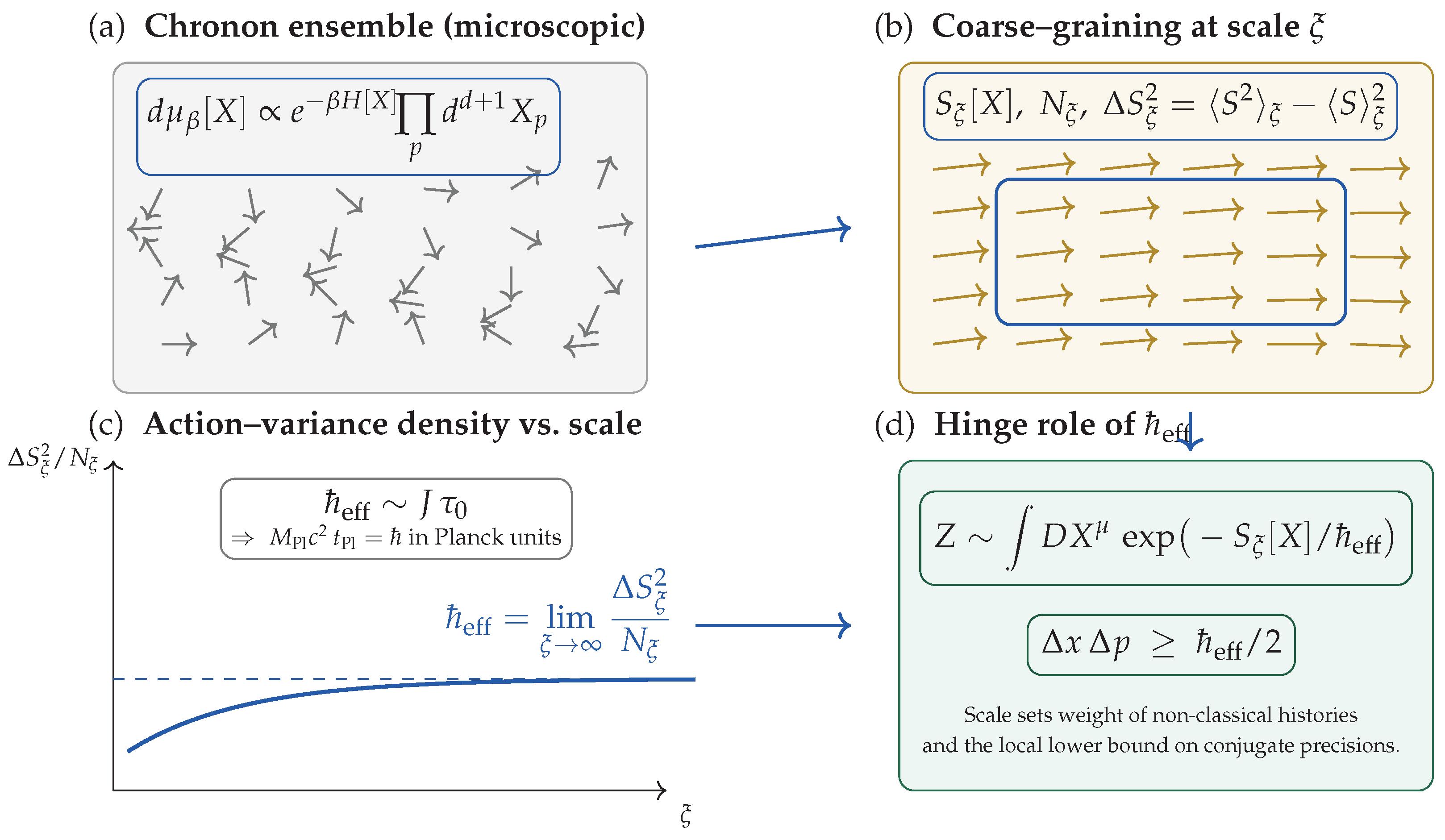
Appendix I.4. Rigorous Derivation of the CFT Uncertainty Bound
In Section 9 we stated Theorem 21, asserting that the uncertainties of canonically conjugate observables in Chronon Field Theory admit a universal lower bound set by the emergent Planck scale . Here we provide the rigorous derivation.
Theorem I.1
(CFT uncertainty for conjugate pairs on a stabilized leaf). Let be a smooth foliation orthogonal to in a stabilized domain, and let be a twice Fréchet–differentiable effective action at coarse–graining scale ξ with strictly hyperbolic linearization. Denote by the retarded/advanced Green’s operators for the linearized Euler–Lagrange operator and by
the Peierls bracket on sufficiently regular functionals . Define quasi–local relational observables on a leaf by
where is the leaf coordinate functional, the Noether stress tensor of , and a positive mollifier of width ξ. Assume further that leaf translations along are symmetries up to errors. Then:
(i) .
(ii) With as in Appendix I, the emergent commutator satisfies .
(iii) Hence the Robertson–Schrödinger inequality yields
If are not canonically conjugate in the above sense (i.e., at leading order), no universal -scaled lower bound exists; only model-dependent covariance terms remain.
Proof. (i) By Noether’s theorem for leaf translations, , where is the generator of -translations. Since shifts as , one obtains . Replacing by its mollified changes the bracket only by , giving (i).
(ii) Consider the coarse–grained path measure . Schwinger–Dyson identities imply
for quasi–local observables . Applying this to , and using (i) yields (ii).
(iii) The Robertson–Schrödinger inequality applied to and gives
Discarding the nonnegative anticommutator term and inserting (ii) establishes the claim. □
Appendix I.5. Future Directions
A full computation of requires specifying the chronon interaction Hamiltonian , the correlation structure of , and the boundary-induced alignment conditions. Numerical studies on discrete chronon lattices may enable extraction of as a scaling limit [17,96], allowing direct comparison with the physical value of Planck’s constant.
This approach offers a pathway to deriving quantum action scales from spacetime-level statistics without postulating quantization a priori.
Appendix J. Double–Slit Experiment in Chronon Field Theory: Rigorous Formulation
Appendix J.1. Set-Up and Objects of the Model
Let be the microscopic chronon field, and its coarse-grained, unit-norm alignment field where stabilized. Two narrow path world-tubes connect source to screen points . Define the fine-grained two-point correlator
We say the two paths are bias-phase coherent at scale ℓ if the cross-path kernel
exceeds a threshold set by instrument noise; projects the phase-relevant components (defined by the local frame). Intuitively, measures whether the local potential average alignments along the two paths preserve a mutual phase reference across the slit separation.
Appendix J.2. Amplitude Composition and Fringe Visibility
Let denote bias-compatible thread families through slit i; define the CFT amplitude at as a restricted path integral over histories compatible with the -induced causal structure:
Here encodes stability of bias correlation along . The screen intensity
is conveniently written as
with phase difference determined by geometric/optical path data and
where the sesquilinear pairing is induced by the foliation (Appendix N). In our framework,
separating generic phase diffusion from the ancestry overlap induced by .
Interference requires to remain near unity, i.e., persistent cross-path bias correlation at the experiment’s scale. This is the rigorous version of the narrative in Section 5 that “interference occurs when local potential average alignments remain sufficiently correlated across both paths.”
Appendix K. Entanglement from Φ-Ancestry: Rigorous Formulation and Solvable Model
Appendix K.1. Formal Definition of Φ-Ancestry
Let be the fine-grained chronon two-point correlation function
Two coarse-grained world-tubes are said to share a Φ-ancestry if there exists a connected spacetime region in their common past such that
for some fixed .
In CFT, two subsystems prepared in the same ancestry region are correlated because their local bias orientations are statistically dependent:
We retain local parameter independence:
and no-signalling:
but relax measurement independence:
Appendix K.2. Solvable Toy Model
Setup.
Consider a microscopic chronon field on Minkowski space. Let be a preparation region in the common past of detectors A and B. Define the hidden variable as the coarse statistic of over . Apparatus settings may be statistically dependent on n via the shared ancestry.
Outcomes are
with zero-mean, independent noises, symmetric about zero, and independent across sites given n.
Measurement-Dependence Channel.
Let
a product of von Mises–Fisher factors, with concentration tuning the ancestry strength. recovers measurement independence; yields perfect correlation with settings.
Appendix K.3. No-Signalling
Because are symmetric and independent of the remote setting given n,
and the model respects operational no-signalling.
Appendix K.4. Correlator and Clauser–Horne–Shimony–Holt Inequality (CHSH)
In the noiseless limit,
As , this integral yields the quantum singlet form , giving
for the standard quadruple of settings. The minimal to achieve can be determined numerically.
Appendix K.5. Theorem Statements
Theorem K.1
(Bell violation with ancestry). For any there exists such that in the above model.
Proposition A1
(No-signalling). Under symmetric, independent noise , the marginals obey and for all .
Corollary A2
(Quantum limit). In the limit and vanishing noise, and .
Appendix K.6. Continuum Anchor
The same structure can be realised by taking to be a stationary random field with spectral weight and defining as a low-pass filter . Finite correlation length and common past volume determine the effective .
Appendix K.7. Numerical Recipe
Sample , draw , compute , and average to estimate E and as a function of .
Appendix L. Derivation of the Born Rule in CFT
In CFT, measurement can be viewed as an unbiased competition among several possible alignments of a microscopic system with the stable field of an apparatus. The system begins with statistical tendencies toward different outcomes; during interaction one tendency eventually locks in while the others fade. Because the process has no built-in bias, the chance of each outcome is fixed by its initial weight, and repeated trials make the observed frequencies concentrate around these values. What appears as “collapse” is thus the stabilization of one alignment, with the Born rule emerging as the unique statistical law of this competition.
We summarize here the main rigorous results of Ref. [70], restated in a compact theorem–proof format.
Assumptions X.1–X.4. (Apparatus domains, interface coupling, detailed balance, observer axioms.)
Theorem L.1
(Simplex diffusion limit). Under Assumptions X.1–X.4, the overlap vector converges in law to a diffusion on with generator
The vertices are absorbing.
Theorem L.2
(Born rule via martingale absorption). Each coordinate is a bounded martingale up to the absorption time τ, hence
Thus the probability of outcome i equals the initial overlap .
Theorem L.3
(Frequency large deviations). For N repeated trials, the empirical frequency vector satisfies a large deviation principle with rate function
minimized uniquely at .
Full details: For complete derivations and mathematical proofs, see Ref. [70].
Appendix M. Philosophical Implications of Chronon Field Theory
Chronon Field Theory (CFT) is not intended as a mere re–packaging of quantum mechanics. Its central postulate—now supported by rigorous results in Appendices A and B—is that a single dynamical, future–directed timelike field generates temporal order and builds the effective spacetime geometry. Appendix A (Ref. [69]) shows that the unit–norm property and Lorentzian signature can emerge dynamically from a broad class of chronon models, while Appendix L (Ref. [70]) derives the Born rule from CFT’s statistical–geometric structure. These results place CFT outside the conceptual starting points of most current interpretations. Here we outline five broad implications.
Appendix M.1. Time and Geometry as Built, Not Given
In standard approaches, time is an external parameter and geometry a fixed background. CFT inverts this: both temporal flow and causal structure arise from the integral curves and local orientation of . This resonates with temporal relationalism [8,88], but here the mechanism is explicitly field–theoretic. Within an otherwise Lorentzian manifold, neither time direction nor foliation is fixed a priori; both emerge dynamically from chronon–field stabilization and can fluctuate or fail at sufficiently small scales. At the microscopic level, the unit–norm property is no longer a postulate but a derived coarse–grained feature (Appendix H), making the existence of a stable time direction a contingent dynamical fact.
Appendix M.2. Causality Without Collapse or Branching
In CFT, causal order and metric structure are outcomes of a stabilized , not abstract bookkeeping devices. A measurement is the local, scale–dependent transition from a fluctuating micro–domain to the macro–coherent of an apparatus. This transition is physical: it embeds a “fuzzy” causal patch into a larger ordered geometry.
On this account, quantum “nonlocality” requires neither superluminal signalling nor the ontology of Many–Worlds. Correlations propagate within the causal network defined by [84]; measurement is the joining of two causal patches, not an instantaneous update of a global wavefunction.
Appendix M.3. Objectivity After the Quantum
Where QBism [41] and Relational QM [87] tie the quantum state to agents, CFT retains an agent–independent ontology. and the geometry it defines exist whether or not they are observed. The wavefunction is tied to the foliation induced by , but that foliation is a physical feature, not a belief–state. Measurement is a geometric reconfiguration of spacetime’s causal fabric, not an observer’s information update, preserving objective realism [33,72] in a Lorentz–covariant setting.
Appendix M.4. Probability as Large–Scale Pattern
In CFT, probabilities reflect the ensemble of chronon–field configurations—and hence local geometries—compatible with given boundaries. Randomness is not fundamental; it emerges from coarse–graining over admissible causal–geometric configurations. Appendix L shows that, in the semiclassical limit, this reproduces the Born rule exactly; in partially stabilized regimes, it predicts calculable deviations, offering potential empirical tests. This fits with Humean approaches [71] where probabilistic laws summarise stable patterns in the actual world.
Appendix M.5. Ontological Economy
CFT avoids the proliferation of worlds of Everett [34], the dual ontology of Bohmian mechanics [16], and the subjectivism of QBism [41]. Its single fundamental entity is the chronon field; time, causal order, and effective geometry are all emergent features of its dynamics. This fits naturally with a field–realist stance [66], in which the ontology consists solely of fields and their interactions.
Appendix M.6. In Summary
CFT’s conceptual commitments can be summarised as:
- Time: local, dynamical, scale–dependent, generated by ;
- Causality & geometry: intrinsic to the field’s structure;
- Measurement: physical stabilization of geometry, not epistemic act;
- Probability: derived geometric–statistical law (Born rule in the stabilized limit);
- Reality: field–theoretic, covariant, observer–independent.
In this light, CFT offers a realist re–framing of quantum theory, treating spacetime structure as something the quantum world constructs from within, rather than something imposed from without.
References
- Aharonov, Y., Albert, D.Z., and Vaidman, L., 1988. How the result of a measurement of a component of the spin of a spin- particle can turn out to be 100. Physical Review Letters, 60(14), pp.1351–1354. [CrossRef]
- Anderson, M.H., Ensher, J.R., Matthews, M.R., Wieman, C.E., and Cornell, E.A., 1995. Observation of Bose–Einstein condensation in a dilute atomic vapor. Science, 269(5221), pp.198–201. [CrossRef]
- Arnowitt, R., Deser, S., and Misner, C.W., 1962. The dynamics of general relativity. In Gravitation: An Introduction to Current Research, pp.227–265. Wiley.
- Aspelmeyer, M., Kippenberg, T.J., and Marquardt, F., 2014. Cavity optomechanics. Reviews of Modern Physics, 86(4), pp.1391–1452. [CrossRef]
- A. Ashtekar and R. S. Tate, “An algebraic extension of Dirac quantization: Examples,” J. Math. Phys., 35, 6434 (1993). [CrossRef]
- Ashtekar, A. and Schilling, T.A., 1999. Geometrical formulation of quantum mechanics. In On Einstein’s Path, pp.23–65. Springer.
- Ballentine, L.E., 1970. The statistical interpretation of quantum mechanics. Reviews of Modern Physics, 42(4), pp.358–381. [CrossRef]
- Barbour, J., 1999. The End of Time. Oxford University Press.
- Barbour, J., 2014. The Janus point: A new theory of time. arXiv:1409.0917.
- Bassi, A. and Ghirardi, G.C., 2003. Dynamical reduction models. Physics Reports, 379(5–6), pp.257–426. [CrossRef]
- Becchi, C., Rouet, A., and Stora, R., 1976. Renormalization of the abelian Higgs–Kibble model. Communications in Mathematical Physics, 42(2), pp.127–162.
- Bell, J.S., 1964. On the Einstein Podolsky Rosen paradox. Physics Physique Fizika, 1(3), pp.195–200. [CrossRef]
- Bell, J.S., 1990. Against “measurement”. Physics World, 3(8), pp.33–40.
- Berry, M.V., 1984. Quantal phase factors accompanying adiabatic changes. Proceedings of the Royal Society A, 392(1802), pp.45–57. [CrossRef]
- Binney, J.J., Dowrick, N.J., Fisher, A.J., and Newman, M.E.J., 1992. The Theory of Critical Phenomena: An Introduction to the Renormalization Group. Oxford University Press.
- Bohm, D., 1952. A suggested interpretation of the quantum theory in terms of “hidden” variables. I and II. Physical Review, 85(2), pp.166–193. [CrossRef]
- Bombelli, L., Lee, J., Meyer, D., and Sorkin, R.D., 1987. Space–time as a causal set. Physical Review Letters, 59(5), pp.521–524. [CrossRef]
- Bohr, N., 1928. The quantum postulate and the recent development of atomic theory. Nature, 121, pp.580–590.
- J. Butterfield, “Laws, causation and dynamics at different levels,” Interface Focus, 2, 101–114 (2012). [CrossRef]
- Callender, C., 2017. What Makes Time Special? Oxford University Press.
- Cariñena, J.F., Clemente-Gallardo, J., and Marmo, G., 2007. Geometrization of quantum mechanics. Theoretical and Mathematical Physics, 152(1), pp.894–903.
- Caves, C.M., 1980. Quantum–mechanical noise in an interferometer. Physical Review D, 23(8), pp.1693–1708. [CrossRef]
- Chaikin, P.M. and Lubensky, T.C., 1995. Principles of Condensed Matter Physics. Cambridge University Press.
- Coleman, S., Wess, J., and Zumino, B., 1969. Structure of phenomenological Lagrangians. I. Physical Review, 177(5), pp.2239–2247. [CrossRef]
- Cronin, A.D., Schmiedmayer, J., and Pritchard, D.E., 2009. Optics and interferometry with atoms and molecules. Reviews of Modern Physics, 81(3), pp.1051–1129. [CrossRef]
- DeWitt, B.S., 1973. The Many-Worlds Interpretation of Quantum Mechanics. Princeton University Press.
- Deutsch, D., 1999. Quantum theory of probability and decisions. Proceedings of the Royal Society A, 455(1988), pp.3129–3137. [CrossRef]
- Dirac, P.A.M., 1930. The Principles of Quantum Mechanics. Oxford University Press.
- Dirac, P.A.M., 1958. The theory of gravitation in Hamiltonian form. Proceedings of the Royal Society A, 246(1246), pp.333–343. [CrossRef]
- Dirac, P.A.M., 1964. Lectures on Quantum Mechanics. Belfer Graduate School of Science, Yeshiva University.
- Dittrich, B., 2007. Partial and complete observables for Hamiltonian constrained systems. General Relativity and Gravitation, 39, pp.1891–1927.
- Dowker, F., 2005. Causal sets and the deep structure of spacetime. In A. Ashtekar (ed.), 100 Years of Relativity, pp.445–464. World Scientific.
- Einstein, A., Podolsky, B., and Rosen, N., 1935. Can quantum–mechanical description of physical reality be considered complete? Physical Review, 47(10), pp.777–780. [CrossRef]
- Everett, H., 1957. “Relative state” formulation of quantum mechanics. Reviews of Modern Physics, 29(3), pp.454–462. [CrossRef]
- Faddeev, L.D. and Popov, V.N., 1967. Feynman diagrams for the Yang–Mills field. Physics Letters B, 25(1), pp.29–30. [CrossRef]
- Feynman, R.P., Leighton, R.B., and Sands, M., 1965. The Feynman Lectures on Physics, Vol. 3. Addison–Wesley.
- Feynman, R.P. and Hibbs, A.R., 2010. Quantum Mechanics and Path Integrals. Dover Publications (updated ed.).
- Frobenius, G., 1877. Über das Pfaffsche Problem. Journal für die reine und angewandte Mathematik, 82, pp.230–315.
- Fröhlich, J., 1981. Mathematical aspects of the physics of disordered systems. In Les Houches Session XXXIX, North-Holland.
- Fuchs, C.A., 2010. QBism, the Perimeter of Quantum Bayesianism. arXiv:1003.5209.
- Fuchs, C.A., Mermin, N.D., and Schack, R., 2014. An introduction to QBism with an application to the locality of quantum mechanics. American Journal of Physics, 82(8), pp.749–754. [CrossRef]
- Gambini, R. and Pullin, J., 2009. Relational physics with real rods and clocks and the measurement problem. Foundations of Physics, 39(11), pp.1143–1155.
- Gell-Mann, M. and Hartle, J.B., 1990. Quantum mechanics in the light of quantum cosmology. In W.H. Zurek (ed.), Complexity, Entropy, and the Physics of Information. Addison–Wesley.
- M. Gell-Mann and J. B. Hartle, “Classical equations for quantum systems,” Phys. Rev. D, 47, 3345 (1993), arXiv:gr-qc/9210010.
- F. Girelli and E. R. Livine, “Reconstructing quantum geometry from quantum information: Spin networks as harmonic oscillators,” Class. Quantum Grav., 23, 7521–7545 (2006).
- Ghirardi, G.C., Rimini, A., and Weber, T., 1986. Unified dynamics for microscopic and macroscopic systems. Physical Review D, 34(2), pp.470–491. [CrossRef]
- Gleason, A.M., 1957. Measures on the closed subspaces of a Hilbert space. Journal of Mathematics and Mechanics, 6(6), pp.885–893.
- F. Gliozzi and F. Capra, “Effective actions from microscopic ensembles: a statistical field theory perspective,” JHEP 2023, 76 (2023), arXiv:2301.07104.
- Goldenfeld, N., 1992. Lectures on Phase Transitions and the Renormalization Group. Addison–Wesley.
- Halperin, B.I., Lubensky, T.C., and Ma, S.-K., 1974. First-order phase transitions in superconductors and smectic-A liquid crystals. Physical Review Letters, 32(6), pp.292–295. [CrossRef]
- Halliwell, J.J., 1995. A review of the decoherent histories approach to quantum mechanics. Annals of the New York Academy of Sciences, 755(1), pp.726–740.
- Hardy, L., 2005. Probability theories with dynamic causal structure: A new framework for quantum gravity. arXiv:gr-qc/0509120.
- Hardy, L., 2007. Towards quantum gravity: a framework for probabilistic theories with non-fixed causal structure. Journal of Physics A, 40(12), pp.3081–3099. [CrossRef]
- Harrigan, N. and Spekkens, R.W., 2010. Einstein, incompleteness, and the epistemic view of quantum states. Foundations of Physics, 40(2), pp.125–157.
- Hawking, S.W. and Ellis, G.F.R., 1973. The Large Scale Structure of Space–Time. Cambridge University Press.
- Heisenberg, W., 1927. Über den anschaulichen Inhalt der quantentheoretischen Kinematik und Mechanik. Zeitschrift für Physik, 43, pp.172–198.
- Heisenberg, W., 1955. The Physical Principles of the Quantum Theory. Dover Publications.
- Hensen, B., et al., 2015. Loophole-free Bell inequality violation using electron spins separated by 1.3 kilometres. Nature, 526, pp.682–686.
- Henneaux, M. and Teitelboim, C., 1992. Quantization of Gauge Systems. Princeton University Press.
- Isham, C.J., 1992. Canonical quantum gravity and the problem of time. In Integrable Systems, Quantum Groups, and Quantum Field Theories, pp.157–287. Springer.
- Joos, E. and Zeh, H.D., 1985. The emergence of classical properties through interaction with the environment. Zeitschrift für Physik B, 59(2), pp.223–243.
- Joos, E., Zeh, H.D., Kiefer, C., Giulini, D., Kupsch, J., and Stamatescu, I.-O., 2003. Decoherence and the Appearance of a Classical World in Quantum Theory (2nd ed.). Springer.
- Kent, A., 2020. Quanta and reality: Selected talks by Ghirardi, Leggett, and Zeh. Foundations of Physics, 50, pp.176–192.
- Kibble, T.W.B., 1979. Geometrization of quantum mechanics. Communications in Mathematical Physics, 65(2), pp.189–201.
- Kuchař, K.V., 1992. Time and interpretations of quantum gravity. In Proceedings of the 4th Canadian Conference on General Relativity and Relativistic Astrophysics, pp.211–314.
- Ladyman, J. and Ross, D., 2007. Every Thing Must Go: Metaphysics Naturalized. Oxford University Press.
- Landau, L.D. and Lifshitz, E.M., 1958. Statistical Physics, Part 1. Pergamon Press.
- Lee, J.M., 2013. Introduction to Smooth Manifolds (2nd ed.). Springer.
- Li, B., 2025. Emergence and Exclusivity of Lorentzian Signature and Unit–Norm Time from Random Chronon Dynamics, preprint, Zenodo. [CrossRef]
- Li, B., 2025. Deriving the Born Rule from Boundary–Induced Alignment in Chronon Field Theory, preprint, Zenodo. [CrossRef]
- Loewer, B., 2004. David Lewis’s Humean theory of objective chance. Philosophy of Science, 71(5), pp.1115–1125. [CrossRef]
- Maudlin, T., 2019. Philosophy of Physics: Quantum Theory. Princeton University Press.
- Misner, C.W., Thorne, K.S., and Wheeler, J.A., 1973. Gravitation. W.H. Freeman.
- Y. J. Ng, “Selected topics in Planck-scale physics,” Mod. Phys. Lett. A, 18, 1073–1097 (2003), arXiv:gr-qc/0305019.
- Oeckl, R., 2003. A “general boundary” formulation for quantum mechanics and quantum gravity. Physics Letters B, 575(3–4), pp.318–324. [CrossRef]
- O’Neill, B., 1983. Semi–Riemannian Geometry with Applications to Relativity. Academic Press.
- Oriti, D., 2014. Group field theory and loop quantum gravity. In Loop Quantum Gravity: The First 30 Years, pp.125–155. World Scientific.
- Oreshkov, O., Costa, F., and Brukner, Č., 2012. Quantum correlations with no causal order. Nature Communications, 3, 1092.
- T. Padmanabhan, “Lessons from Classical Gravity about the Quantum Structure of Spacetime,” J. Phys. Conf. Ser., 306, 012001 (2011), arXiv:1012.4476.
- Page, D.N. and Wootters, W.K., 1983. Evolution without evolution: Dynamics described by stationary observables. Physical Review D, 27(12), pp.2885–2892. [CrossRef]
- Perez, A., 2013. The spin–foam approach to quantum gravity. Living Reviews in Relativity, 16(1), p.3.
- Peres, A. and Terno, D.R., 2002. Quantum information and relativity theory. Reviews of Modern Physics, 76(1), pp.93–123. [CrossRef]
- Pikovski, I., Zych, M., Costa, F., and Brukner, Č., 2015. Universal decoherence due to gravitational time dilation. Nature Physics, 11(8), pp.668–672.
- Price, H. and Wharton, K., 2015. Disentangling the quantum world. Entropy, 17(11), pp.7752–7767. [CrossRef]
- H. P. Robertson, “The Uncertainty Principle,” Phys. Rev., 34, 163–164 (1929).
- Rovelli, C., 1990. Quantum mechanics without time: A model. Physical Review D, 42(8), pp.2638–2646. [CrossRef]
- Rovelli, C., 1996. Relational quantum mechanics. International Journal of Theoretical Physics, 35(8), pp.1637–1678.
- Rovelli, C., 2004. Quantum Gravity. Cambridge University Press.
- Rovelli, C. and Smolin, L., 1990. Loop space representation of quantum general relativity. Nuclear Physics B, 331(1), pp.80–152. [CrossRef]
- Sakurai, J.J., 1995. Modern Quantum Mechanics. Addison–Wesley.
- Saunders, S., Barrett, J., Kent, A., and Wallace, D. (eds.), 2010. Many Worlds? Everett, Quantum Theory, and Reality. Oxford University Press.
- Schlosshauer, M., 2007. Decoherence and the Quantum–to–Classical Transition. Springer.
- Schrödinger, E., 1935. Die gegenwärtige Situation in der Quantenmechanik. Naturwissenschaften, 23, pp.807–812; 823–828; 844–849. [CrossRef]
- Schwinger, J., 1948. Quantum electrodynamics. I. A covariant formulation. Physical Review, 74(10), pp.1439–1461. [CrossRef]
- R. D. Sorkin, “Causal sets: Discrete gravity (Notes for the Valdivia summer school),” Lectures on Quantum Gravity, Springer, 2005, arXiv:gr-qc/0309009.
- Surya, S., 2019. The causal set approach to quantum gravity. Living Reviews in Relativity, 22(1), p.5.
- Sundermeyer, K., 1982. Constrained Dynamics. Springer.
- Teitelboim, C., 1983. The Hamiltonian structure of space–time. In General Relativity and Gravitation, pp.195–225. Plenum Press.
- Tegmark, M., 1998. The interpretation of quantum mechanics: Many worlds or many words? Fortschritte der Physik, 46(6–8), pp.855–862.
- Tomonaga, S., 1946. On a relativistically invariant formulation of the quantum theory of wave fields. Progress of Theoretical Physics, 1(2), pp.27–42. [CrossRef]
- Tyutin, I.V., 1975. Gauge invariance in field theory and statistical physics in operator formalism. Lebedev Physics Institute preprint 39.
- von Neumann, J., 1932. Mathematische Grundlagen der Quantenmechanik. Springer.
- von Neumann, J., 1955. Mathematical Foundations of Quantum Mechanics. Princeton University Press.
- Wald, R.M., 1984. General Relativity. University of Chicago Press.
- Wald, R.M., 1994. Quantum Field Theory in Curved Spacetime and Black Hole Thermodynamics. University of Chicago Press.
- Wallace, D., 2012. The Emergent Multiverse: Quantum Theory According to the Everett Interpretation. Oxford University Press.
- Weinberg, S., 1989. Testing quantum mechanics. Annals of Physics, 194(2), pp.336–386. [CrossRef]
- Weinberg, S., 1996. The Quantum Theory of Fields, Vol. II: Modern Applications. Cambridge University Press.
- Wheeler, J.A., 1957. On the nature of quantum geometrodynamics. Annals of Physics, 2(6), pp.604–614. [CrossRef]
- Wheeler, J.A., 1978. The “past” and the “delayed-choice” double-slit experiment. In A.R. Marlow (ed.), Mathematical Foundations of Quantum Theory, pp.9–48. Academic Press.
- Wheeler, J.A., 1984. Law without law. In J.A. Wheeler and W.H. Zurek (eds.), Quantum Theory and Measurement, pp.182–213. Princeton University Press.
- Wheeler, J.A. and Zurek, W.H. (eds.), 1983. Quantum Theory and Measurement. Princeton University Press.
- Wood, C.J. and Spekkens, R.W., 2015. The lesson of causal discovery algorithms for quantum correlations: Causal explanations of Bell-inequality violations require fine-tuning. New Journal of Physics, 17(3), 033002.
- Yin, J., et al., 2017. Satellite-based entanglement distribution over 1200 kilometers. Science, 356(6343), pp.1140–1144. [CrossRef]
- Zurek, W.H., 2003. Decoherence, einselection, and the quantum origins of the classical. Reviews of Modern Physics, 75(3), pp.715–775. [CrossRef]
- Zurek, W.H., 2005. Probabilities from entanglement, Born’s rule from envariance. Physical Review A, 71(5), 052105. [CrossRef]
Figure 2.
Schematic: -threads propagate causally through both slits, guiding the quantum system toward interference regions. This is an interpretive model; a derivation from the CFT action remains to be worked out.
Figure 2.
Schematic: -threads propagate causally through both slits, guiding the quantum system toward interference regions. This is an interpretive model; a derivation from the CFT action remains to be worked out.
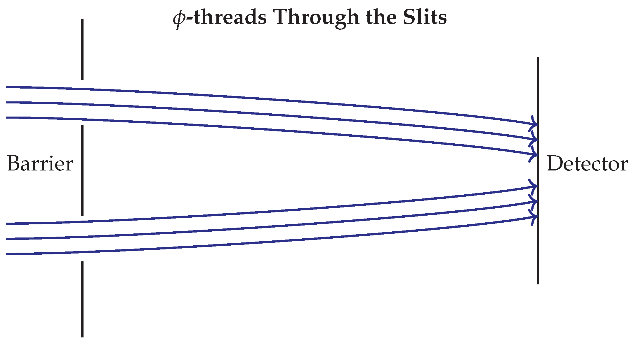
Figure 3.
Which–path detection as boundary–induced alignment in CFT. The –thread through the upper slit enters the detector’s ordered –domain (green) and is dynamically aligned to its causal geometry (solid green trajectory). Its original phase orientation (blue ticks) is replaced by the detector’s aligned phase (green ticks), breaking phase correlation with the lower slit path (blue). The lower path retains local –coherence but no longer shares a common phase reference with the upper path, eliminating interference. No nonlocal collapse is invoked; the loss of interference is a causal–geometric consequence of embedding a locally coherent micro–domain into a macro–coherent causal structure.
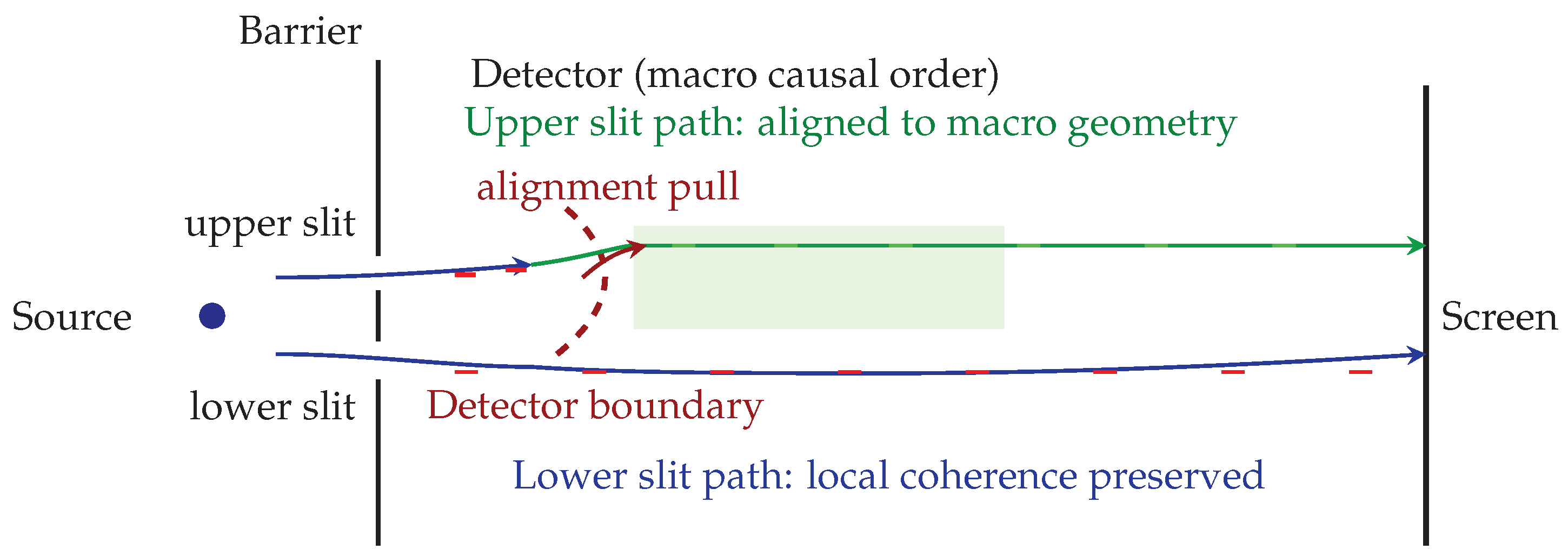
Figure 4.
CFT view of Schrödinger’s cat. The microdomain has several short–range causal threads (red, dashed). After interaction, it aligns with the macro–coherent (blue, solid), inheriting its time direction. Inside the cat’s domain, one outcome exists throughout; for an external observer, that outcome is only identified once causal contact is made.
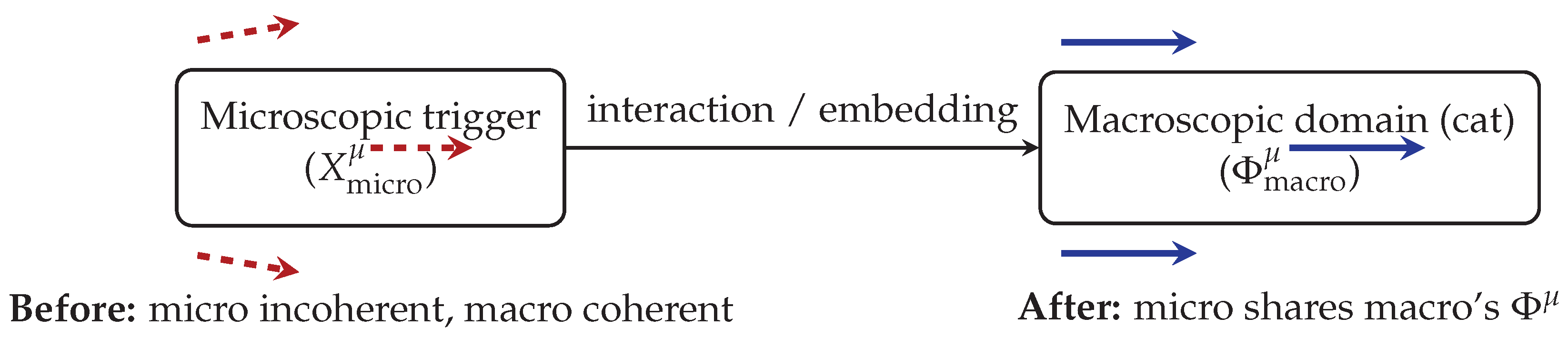
Figure 5.
CFT view of entanglement. The curved layers are intrinsic foliation surfaces of constant proper time defined by the coarse–grained . Events A and B are spacelike–separated detections, each with its own local light cone (, ). They remain correlated because both originate from a shared Φ ancestry region in which their –threads formed a single topologically coherent structure. The correlations violating Bell inequalities are a feature of this pre–existing geometry, not the result of superluminal influence or branching worlds.
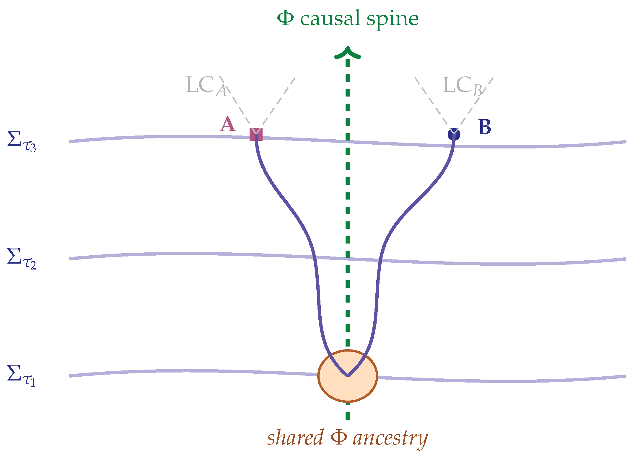
Figure 6.
Emergent uncertainty in CFT. (a) Microscopic domain with incoherent chronon biases : large variance , no stable foliation. (b) Mesoscopic domain: partial alignment reduces variance and begins to define . (c) Macroscopic domain: coherent, unit–norm yields classical records. (d) As coherence increases, the uncertainty product approaches a lower bound governed by the locally emergent ; the inset covariance ellipse depicts spatial variance.
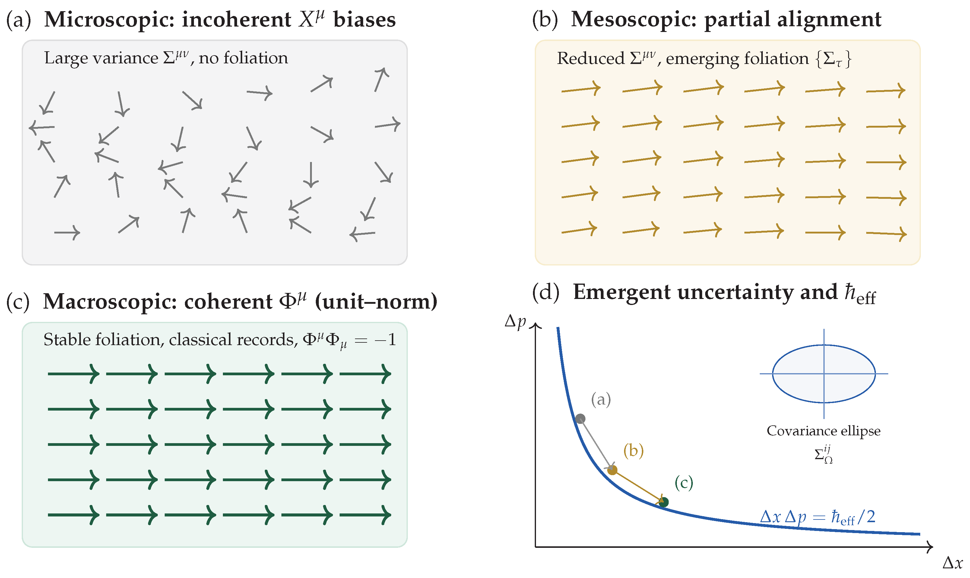
Disclaimer/Publisher’s Note: The statements, opinions and data contained in all publications are solely those of the individual author(s) and contributor(s) and not of MDPI and/or the editor(s). MDPI and/or the editor(s) disclaim responsibility for any injury to people or property resulting from any ideas, methods, instructions or products referred to in the content. |
© 2025 by the authors. Licensee MDPI, Basel, Switzerland. This article is an open access article distributed under the terms and conditions of the Creative Commons Attribution (CC BY) license (http://creativecommons.org/licenses/by/4.0/).
Copyright: This open access article is published under a Creative Commons CC BY 4.0 license, which permit the free download, distribution, and reuse, provided that the author and preprint are cited in any reuse.


