Submitted:
26 August 2025
Posted:
28 August 2025
You are already at the latest version
Abstract
We derive the Born rule in Chronon Field Theory (ChFT) from first principles under realistic measurement assumptions. A recent work in ChFT shows that Lorentzian signature and causal structure emerge dynamically from a unit–norm constraint on the chronon field, providing the geometric foundation for the time–asymmetric alignment dynamics studied here. First, we obtain a diffusion limit for alignment order parameters on the outcome simplex and prove that the overlaps with apparatus eigen–domains form martingales up to the absorption time; optional stopping then yields single–shot Born probabilities. Second, we derive the stochastic limit from noisy chronon gradient flow with boundary coupling by a hydrodynamic limit (tightness, identification of the generator, and boundary layer analysis). Third, we establish a large–deviation principle for empirical frequencies in repeated measurements via Sanov’s theorem, with rate function minimized at the Born vector. We quantify robustness to finite temperature, imperfect interfaces, and basis degeneracies, and outline falsifiable predictions for alignment timescales and drift bounds. Conceptually, the analysis shows that measurement is not a collapse of the system into one of its own eigenstates, but stochastic absorption of the system field into pre–stabilized apparatus eigen–domains. This does not directly contradict the standard textbook view—since apparatus domains are engineered to correspond to system eigenbases—but offers a deeper dynamical interpretation of why outcomes are definite and Born–weighted.
Keywords:
born rule
; chronon field theory
; stochastic processes
; hydrodynamic limit
; large deviations
; Sanov’s theorem
; quantum foundation
1. Introduction
Motivation.
Chronon Field Theory (ChFT) models quantum measurement as boundary–induced alignment, in which a microscopic chronon domain with weakly correlated orientations couples across an interface to a macroscopic apparatus region whose coarse–grained field is stabilized (future–directed, unit–norm, twist–free). This coupling drives the domain’s effective field into alignment with one of a finite set of apparatus eigen–domains, yielding a definite outcome without invoking nonlocal collapse. Prior work established that the Lorentzian, unit–norm phase is both exclusive and selected by measurement within apparatus regions, and showed that this phase emerges dynamically from a global unit–norm constraint on the chronon field in flat configuration space, thereby grounding causal structure and temporal asymmetry in the intrinsic geometry of the field space [63]. A key remaining challenge, and the focus of this paper, is to derive the Born rule—the quadratic dependence of outcome probabilities on initial amplitudes—from chronon dynamics alone, without introducing additional probabilistic axioms.
Conceptual mechanism.
At the core of CFT is a field-theoretic model of quantum measurement in which outcome selection emerges from alignment geometry at the apparatus boundary. The apparatus defines a finite set of stabilized pointer configurations—the eigen–domains—with which the chronon field of the microscopic system can stochastically align. This alignment is local and continuous in spacetime, but due to coarse–graining and boundary coupling, the dynamics becomes probabilistic and irreversible on macroscopic scales. The outcome simplex encodes the overlaps between the evolving chronon field and these eigen–domains, and absorption into a vertex corresponds to a definite measurement result. Conceptually, this means that measurement is not a collapse of the system into one of its own eigenstates, but absorption of the system field into apparatus eigen–domains that are engineered to correspond to the system’s eigenbasis. This does not contradict the standard textbook view, but reframes it: the apparatus, rather than the system, selects the effective measurement basis, yielding both outcome definiteness and Born weights from physical chronon dynamics without postulates.
Objective.
This paper provides an operational and rigorous derivation of the Born rule in the CFT measurement setting under explicit, verifiable assumptions on the apparatus, interface, and noise. That is, given a system prepared in state and an observable with eigenstates , the probability of obtaining outcome is
We treat the alignment overlaps with apparatus eigen–domains as order parameters,
collectively forming a process on the outcome simplex . Our main results establish that, under boundary–consistent noise and detailed balance at the interface, (i) the coarse–grained chronon dynamics yields a diffusion limit for on with absorbing vertices, (ii) the coordinates are martingales up to the absorption time, and therefore (iii) single–shot absorption probabilities equal the initial overlaps , i.e., the Born weights. We then obtain a large–deviation principle (LDP) for empirical outcome frequencies in repeated trials, with rate function minimized at the Born vector.
Contributions.
In this paper we prove the following:
- Geometric mechanism for outcome selection. We model measurement as stochastic field alignment with a finite family of apparatus eigen–domains, yielding definite outcomes via absorption in the outcome simplex without invoking collapse.
- Simplex diffusion (Theorem 3.1). Starting from a noisy gradient–flow model for with boundary coupling to (consistent with a Gibbs noise model at inverse temperature and interface strength ), we derive, under mild regularity and symmetry assumptions, a diffusion limit for the projected overlap process on with absorbing vertices . The limiting generator has continuous, Lipschitz coefficients and preserves the simplex.
- Martingale structure and Born probabilities (Proposition 17, Theorem 4.1). We show that detailed balance at the interface enforces zero drift for each coordinate: . Hence is a (uniformly integrable) martingale up to the absorption time at the simplex vertices. By optional stopping, the absorption probabilities satisfyyielding the Born rule when are the initial overlaps with the apparatus eigen–domains.
- Collapse as absorption (Section 5). We interpret the selection of a definite measurement outcome as stochastic absorption of the alignment overlap vector at a simplex vertex. This dynamical mechanism replaces the conventional wavefunction collapse postulate with a local, continuous, and probabilistic alignment process, reconciling definiteness of outcomes with causal and reversible dynamics.
- Hydrodynamic grounding (Theorem 6.1). We justify the diffusion approximation by proving tightness of the projected processes under chronon microdynamics, identifying the limit via the martingale problem [31], and computing the covariance from boundary fluctuations through a fluctuation–dissipation relation.
- Frequency large deviations (Theorem 7.1). For repeated measurements prepared with identical initial overlaps, we obtain a Sanov–type LDP for empirical frequencies with good rate function minimized uniquely at [19].
- Robustness bounds (Theorem 8.1). We quantify deviations from Born weights under imperfect interfaces (finite ), finite temperature , and small symmetry–breaking drifts, obtaining explicit perturbative error bounds of the form
Relation to prior work.
Conceptually, our derivation parallels the martingale structure underlying stochastic Schrödinger equations and quantum trajectories [3,94], but differs in two essential ways: (i) the stochasticity arises from classical chronon fluctuations at the apparatus boundary within CFT’s emergent causal geometry, rather than from postulated stochastic modifications to Schrödinger evolution; (ii) the simplex diffusion and its zero–drift property are derived from interface detailed balance and symmetry of the alignment energy, not imposed.
Compared to objective collapse models [6,39], our approach does not introduce new dynamical laws or coupling constants. Relative to purely epistemic accounts [13,84], outcome probabilities here emerge from physical stochastic absorption in the alignment geometry, not knowledge updates. Decoherence-based arguments [99] suppress interference but do not yield definite outcomes or derive Born weights; our model addresses both via the absorbing boundary structure of the outcome simplex.
Finally, unlike decision-theoretic derivations in Everettian settings [20,91], or subjectivist reconstructions such as QBism [34], the present framework grounds the Born rule in a local, emergent field theory with classical causal structure and no branching or agent-centric assumptions. The absorption law is tied directly to macroscopic alignment geometry and fluctuations, offering a new class of explanation distinct from stochastic mechanics [69] or gravitational collapse models [21,76].
Structure of the paper.
Section 2 formalizes the operational setting: apparatus eigen–domains, alignment overlaps, admissible noise, and observer axioms. Section 3 derives the limiting diffusion on the outcome simplex and states the required regularity and symmetry assumptions. Section 4 proves the martingale property and derives single–shot Born probabilities by optional stopping, including hitting and integrability lemmas. Section 6 provides the hydrodynamic limit from chronon microdynamics, establishing tightness and identifying the limiting generator and covariance via boundary fluctuation–dissipation. Section 7 proves the frequency LDP for repeated trials and sketches an alternative thermodynamic LDP via constrained free energies. Section 8 gives quantitative stability bounds and extensions to degeneracies and POVMs. Section 9 outlines experimental and numerical signatures. We conclude with a discussion of open problems and future directions.
To orient the reader, Figure 1 summarizes the logical pipeline/flowchart of our derivation. The starting point is the chronon dynamics in the apparatus boundary layer, modeled as a reversible noisy alignment process. Under suitable mixing and time–scale separation, these microscopic dynamics converge to an effective diffusion for the overlap vector on the outcome simplex. This diffusion is neutral and martingale–valued, so that absorption at the simplex vertices yields outcome probabilities equal to the initial overlaps—precisely the Born rule. At the level of repeated trials, empirical frequencies concentrate at the Born vector according to a large–deviation principle, providing a statistical law of large numbers with exponential accuracy. Finally, realistic imperfections such as finite coupling, temperature, or geometric asymmetry enter only as small drift or covariance corrections, for which quantitative stability bounds are available. In this way the figure provides a schematic overview, connecting microscopic chronon alignment to the emergence and robustness of Born statistics.
For Non-specialists. Because some of our arguments draw on techniques from probability theory, statistical physics, and information theory, we provide a self-contained pedagogical appendix for non-specialist readers. There we review the essential background on martingales and optional stopping, Wright–Fisher diffusions on the simplex, and large deviations via relative entropy and Sanov’s theorem, together with simple examples and diagrams. Readers familiar with these standard tools may skip the appendix.
2. Operational Setup and Measurement Geometry
2.1. Apparatus Eigen–Domains and Alignment Observables
We formalize the macroscopic apparatus, its stabilized alignment field, the measurement interface, and the outcome observables that will generate a process on the outcome simplex.
Definition 1
(Stabilized apparatus domain). An apparatus domain is an open, connected subset equipped with a smooth, future–directed, unit–norm timelike vector field
that is twist–free in :
Consequently, there exists a smooth proper–time function on whose level sets are spacelike hypersurfaces orthogonal to . We call the apparatus foliation.
Remark 2 (Emergent causal structure from chronon constraints).
The apparatus field induces the local causal structure and time direction in by defining a unit–norm, twist–free timelike flow. This structure is not imposed arbitrarily: in a companion analysis [63], it is shown that such Lorentzian signature arises naturally from a unit–norm constraint on the chronon field over a flat background configuration space. There, the kinetic term in the effective action, constrained to preserve unit norm, selects a hyperbolic geometry with a distinguished timelike direction—providing a geometric foundation for the causal alignment process assumed in the present derivation. (See Appendix L for a justification of the eigen–domain structure.)
Definition 3
(Measurement interface and channels). Let be the (mesoscopic) microdomain prepared for measurement, and let be the spacelike measurement interface on a fixed apparatus leaf . Denote by the induced Riemannian metric on and by its volume form.
A family of channels is a measurable partition
with each of positive –measure. Define , so that
We refer to (or ) as the apparatus eigen–domains (resp. an orthonormal channel basis).
Remark 4 (Geometry and physical meaning).
The field fixes the local time direction and causal geometry in (Def. 1). The partition encodes distinct, macroscopically disjoint pointer channels (e.g. separate detector pixels or paths) on the interface where the microdomain first couples to the apparatus. Orthogonality is in the function space , not in Minkowski space; distinct channels are disjoint in space, which is the operational origin of outcome exclusivity [98].
Remark 5 (Channel symmetry and standard QM).
In the present framework, we assume symmetry of the apparatus eigen–domains, so that no outcome channel is intrinsically favored beyond the system’s own overlaps. This assumption is not an additional hypothesis, but rather the field–theoretic restatement of what is already built into the standard measurement postulate: projective measurements treat all eigenstates of a given observable on equal footing, and more generally POVMs require , ensuring completeness and unbiasedness of the outcome channels. In textbook quantum mechanics this symmetry is taken as axiomatic, whereas here it is realized dynamically through the geometry and stochastic alignment of the apparatus domains.
Definition 6
(Alignment scalar and alignment observable). Let be the coarse–grained chronon field in a neighbourhood of . Define the local alignment scalar on by
which satisfies whenever both and are unit–norm, future–directed timelike fields. Let be a fixed strictly increasing function (e.g. ). The channel strengths are
Definition 7
(Alignment overlaps and outcome simplex). Provided , define the alignment overlaps (or overlap vector)
Then takes values in the outcome simplex
Lemma 8
(Normalization, positivity, and continuity).
Under the hypotheses of Definitions 1–7, the map is well–defined on the set where and satisfies:
Remark 9 (Choice of f and invariance).
Any strictly increasing f yields the same ordering of channel strengths and, after normalization, the same up to a continuous, strictly order–preserving reparametrization of the pre–normalized scores. The choice is convenient analytically (smooth, convex) and physically interpretable as a quadratic energy gain from alignment [37].
Remark 10 (Single–point vs. spatially averaged overlaps).
The channel basis (Def. 3) implements a spatial coarse–graining of the local alignment scalar over each channel . This averaging is essential for robustness and for the hydrodynamic limit: it ensures that is insensitive to microscopic fluctuations below the interface scale and provides Lipschitz continuity of the overlaps with respect to in trace norms, which will be used in Section 3, Section 4, Section 4 and Section 6 [85].
Dynamics notation.
2.2. Observer Axioms and Admissible Dynamics
We recall the operational axioms that constrain physically realizable observers and specify the admissible stochastic dynamics for the alignment process at the measurement interface. The axioms ensure causal consistency at the macroscopic level; the dynamics below is an effective description of boundary–driven relaxation in the apparatus and will be shown to imply a diffusion limit for the alignment overlaps on the outcome simplex.
Definition 11
(Observer axioms). An observer is a macroscopic open system supported in a stabilized apparatus domain (Definition 1) whose operation satisfies:
- (O1)
- Well–posed local dynamics. The physical degrees of freedom (matter + fields) obey local second–order PDEs admitting a well–posed Cauchy problem on spacelike slices of the apparatus foliation [47].
- (O2)
- Finite–speed signalling. There exists a cone structure compatible with such that disturbances from compactly supported initial data propagate inside the corresponding domains of dependence.
- (O3)
- Acyclic causal order. The causal precedence relation on is irreflexive and transitive; no closed causal loops exist in the operational regime.
- (O4)
Interface parameters.
We fix an apparatus leaf and a spacelike interface (Definition 3) with orthonormal channel basis . Two control parameters enter the interface model:
The coupling quantifies the energetic penalty for misalignment between and on ; the temperature parameterizes thermal fluctuations of the chronon degrees of freedom in the boundary layer.
Effective alignment functional.
On a neighbourhood U of we consider the coarse–grained functional (bulk + boundary)
with , , (ordered phase).
Definition 12
(Admissible alignment dynamics). An admissible dynamics for near is either of the following two classes:
(H) Hyperbolic (causal) stochastic dynamics. A damped stochastic wave equation on U,
with , where is a space–time Gaussian field of zero mean, white in time and smooth at spatial scale (the boundary microscopic scale), and is a positive self–adjoint mobility operator on U. Boundary condition on :
with outward normal n, Gaussian boundary noise (white in time, smooth on ), and positive self–adjoint boundary mobility .
(P) Overdamped (gradient–flow) stochastic dynamics. An –gradient flow on U,
with boundary condition
where and are positive self–adjoint mobilities (bulk and boundary).
Assumption 13
(Detailed balance and fluctuation–dissipation). In either class (H) or (P), the bulk and boundary mobilities are chosen so that the Markov semigroup of the process is reversible with respect to the Gibbs measure
i.e. detailed balance holds:
where is the generator. Equivalently, the noise covariances satisfy the fluctuation–dissipation relation with the same mobilities that define the drift (class P) or the damping operators (class H).
Assumption 14
(Well–posedness and locality). For class (H), the deterministic part of (2) is strictly hyperbolic with finite propagation speed in ; the stochastic forcing has compact spatial correlation support of diameter , ensuring that for any the influence of data outside the domain of dependence is exponentially suppressed. For class (P), the dynamics (4) is the overdamped limit of (H) on timescales ; it is confined to a thin tubular neighbourhood of of thickness and cannot be used operationally for signalling outside . In both cases, for initial data there exists a unique (probabilistically strong) solution with continuous paths in on finite time intervals.
Remark 15 (Compatibility with observer axioms).
Axioms (O1)–(O3) apply to the macroscopic propagation of matter and information in . Class (H) respects finite–speed propagation at the level of alignment dynamics. Class (P) is an effective, strongly damped limit describing local relaxation of inside the apparatus boundary layer; since it is confined to U and reversible w.r.t. , it does not generate superluminal signalling or causal anomalies at the operational level. Axiom (O4) is ensured by the existence and uniqueness of the minimizer of in the apparatus (stability of records), as established in the measurement selection results.
Consequence for overlaps.
Under Assumptions 13–14, the process (Definition 7) is a Markov process on whose drift is determined by the –reversible dynamics. In Section 3 we prove that, after a diffusive rescaling and projection, converges to a diffusion with absorbing vertices and, by detailed balance, has zero drift along each coordinate—yielding the martingale structure central to our Born–rule derivation.
3. From Noisy Alignment Dynamics to a Simplex Diffusion
3.1. Noisy Gradient Flow for with Boundary Coupling
We work with the overdamped (gradient–flow) class (P) from Definition 12, in the spirit of stochastic gradient flows for SPDEs [17]. Let U be a tubular neighbourhood of the interface . The coarse–grained alignment functional is
with , , fixed.
The stochastic alignment dynamics is the gradient flow of with Gibbs–consistent noise (Assumption 13), consistent with the fluctuation–dissipation framework for SPDEs [45,86]:
where W is a cylindrical Wiener process on with covariance trace–class at spatial scale , B is a boundary Wiener process on with trace–class covariance, and , are positive self–adjoint mobilities. By Assumption 14, for any , (8)–(9) has a unique strong solution with continuous –paths on finite times [17].
Let be the trace operator. Recall the alignment overlaps (Def. 7) built from the local scalar and a fixed strictly increasing :
Set .
To compute the stochastic evolution of we use Itô’s formula for functionals of infinite–dimensional diffusions [17]. If is twice Fréchet differentiable with appropriate growth and trace–class noise, then
We apply and then the quotient rule with . The derivatives and act via the chain rule on restricted to , yielding local multipliers proportional to and .
3.2. Projected Order Parameters and Limiting SDE
The resulting evolution for can be written as
where , are the coordinates of W and B in orthonormal bases, and , , are obtained from , , the mobilities, and the trace. By Assumption 13, the quadratic variation of p is governed by the reversible Dirichlet form of ; is induced by the deterministic part of (8)–(9) plus the Itô correction.
We now perform a diffusive rescaling that averages out fast boundary fluctuations in the alignment layer, following standard diffusion-approximation theory [31]. Fix a scale parameter and define
Under time–scale separation (fast relaxation of at fixed p) and mixing in the boundary layer, weak convergence of to a Markov diffusion p on holds with generator
where the effective covariance and drift are obtained by fluctuation-averaging [73]. Permutation symmetry of channels and invariance under rigid motions preserving imply that has the Wright–Fisher form [31,33]
where is a scalar boundary diffusion intensity. Detailed balance at the interface enforces zero effective drift [86]:
Finally, the absorbing condition at faces follows from standard boundary classification for absorbing Wright–Fisher diffusions [33].
A canonical SDE representation of (11)–(12) is
where is a matrix of independent standard Brownian motions. The form (14) is a standard Wright–Fisher diffusion representation [31,33]; it preserves the simplex constraint and ensures almost surely.
Assumption 16
(Regularity and symmetry). We assume:
- (R1)
- (R2)
- (Boundary mixing & time–scale separation) The alignment layer near is rapidly mixing on time scale ; conditional on p, the fast variables are ergodic with a unique reversible measure induced by , and their autocovariances are integrable, consistent with homogenization theory [73].
- (R3)
- (Channel symmetry) The geometry and noise are invariant under permutations of and under isometries of that preserve ; f is fixed once and for all.
- (R4)
- (Absorbing vertices) If for some i, then the limiting dynamics leaves p at almost surely, in analogy with absorbing boundaries in Wright–Fisher diffusions [33].
Theorem 3.1
(Diffusion limit on the outcome simplex). Let be the rescaled overlap process associated with (8)–(9). Suppose Assumptions 13, 14, and 16 hold. Then, as , the laws of on are tight and converge weakly to the unique solution of the martingale problem for the generator in (11) with covariance (12) and zero drift (13), subject to absorbing boundary condition at the vertices [31,86]. Equivalently, where p solves (14) on with absorption at .
Proof sketch.
Tightness follows from Aldous’ criterion [1] using (R1) and uniform moment bounds derived from the reversible Dirichlet form. Identification of the limit uses the martingale problem framework [31,86]: for smooth f, is a martingale, where is computed from (10). Under (R2), with covariance (12) obtained by Green–Kubo formulas for boundary fluctuations [42], and under detailed balance (Assumption 13) the effective drift vanishes. Absorption (R4) is inherited by the limit. Uniqueness in law for (14) with degenerate diffusion on is standard [31,33]. □
4. Martingale Structure and Absorption Probabilities
4.1. Zero–Drift Structure from Detailed Balance
For the limiting diffusion of Theorem 3.1, detailed balance at the interface (Assumption 13), together with channel symmetry (R3), implies in (11). Intuitively, in the neutral (symmetric) alignment landscape the apparatus does not bias transitions between channels; the stochastic fluctuations are balanced and purely diffusive on [31].
Proposition 17
(Martingale property). Let be the –valued diffusion of Theorem 3.1. Then for each , is a bounded martingale with respect to the natural filtration up to the absorption time . In particular, for all .
4.2. Optional Stopping and Born Weights
Let denote the ith vertex of (the pure ith channel). Define as above.
Theorem 4.1
(Single–shot Born probabilities). Assume the hypotheses of Theorem 3.1 and Proposition 17. Then
If the microdomain is prepared with initial overlaps relative to the apparatus eigen–domains, the absorption probabilities equal the Born weights .
Proof sketch.
See Appendix N for the full proof.
4.3. Hitting, Non-Explosion, and Boundary Behavior
Lemma 18
Proof sketch.
In the neutral Wright–Fisher diffusion with m types and no mutation, standard boundary classification shows that the boundary is attainable and absorbing [31,33]. Successive extinction of types occurs until fixation at a vertex. Lyapunov functions of the form satisfy away from vertices, implying that V is a strict supermartingale and giving finiteness of by Foster–Lyapunov criteria [66]. See Appendix M for details. □
Consequence.
Lemmas 18 and Proposition 17 justify optional stopping in Theorem 4.1 and complete the single–shot Born–rule derivation under the chronon alignment dynamics. See Appendix N for the full proof.
5. Collapse, Definiteness, and the Outcome Simplex
In standard quantum mechanics, the measurement problem centers on how a quantum system, initially described by a coherent superposition, yields a single, definite outcome upon observation. The traditional response is the wavefunction collapse postulate, an explicit discontinuous update to the system’s state conditioned on measurement [90]. This section interprets how Chronon Field Theory (ChFT) resolves this issue dynamically, by replacing postulated collapse with stochastic absorption in the outcome simplex.
5.1. Collapse as Stochastic Absorption
Let denote the time-dependent overlap vector encoding the alignment of the chronon field with the m apparatus eigen–domains (Definition 7). As shown in Proposition 17, each coordinate is a bounded martingale under the interface-coupled chronon dynamics, and the process is absorbed almost surely at one of the simplex vertices in finite time (Lemma 18).
This absorption event corresponds to a physical measurement outcome. Specifically, absorption at implies that channel i dominates the alignment, i.e.,
The field configuration becomes fully aligned with the ith apparatus eigen–domain, and this alignment is macroscopically stable due to the properties of the stabilized apparatus region (Definition 1). Thus, the measurement produces a definite, classically recordable outcome without the need to invoke discontinuous projection or nonlocal effects.
5.2. Comparison to Conventional Collapse
This absorption-based mechanism fulfills the empirical role of wavefunction collapse but arises here as an emergent property of local, reversible, and stochastic dynamics at the boundary layer:
- The outcome is definite due to absorption: the system eventually enters a simplex vertex state , excluding all other outcomes.
- The process is probabilistic via martingale properties: the absorption probabilities are given by the initial overlaps , reproducing the Born rule (Theorem 4.1).
- The dynamics is local and continuous in spacetime: all stochasticity originates from chronon fluctuations at the measurement interface , governed by reversible SPDEs (Section 3).
In contrast to standard collapse models (e.g., GRW [39]), no additional dynamics or modification of Schrödinger evolution is introduced. Unlike purely epistemic views [46,84], the stochasticity arises from an objectively fluctuating alignment process. Compared to quantum trajectory or stochastic Schrödinger frameworks [5,22,40], the present derivation ties the martingale and absorption structure to coarse–grained, classical field interactions, rather than postulating stochasticity at the level of the wavefunction.
5.3. System Eigenstates versus Apparatus Eigen–Domains
In the textbook formulation of quantum measurement, a system initially prepared in a superposition
of eigenstates of some observable O is said to “collapse” into one of these eigenstates upon measurement, with Born probability . The apparatus is then taken to record this outcome by correlating its pointer state with the corresponding eigenstate of the system.
Chronon Field Theory (ChFT) reformulates this picture. In CFT, the apparatus is not a passive recorder but an active dynamical system that defines a finite set of stable, coarse–grained alignment channels, or eigen–domains. The chronon field of the microscopic system couples to these domains across the measurement interface , and its effective alignment process is described by the overlap vector . As shown in Section 5, the overlaps undergo a martingale diffusion and are absorbed almost surely at a simplex vertex , corresponding to one of the apparatus eigen–domains. In this sense, the measurement outcome is realized as absorption of the system’s chronon field into a pre–existing apparatus channel, rather than collapse of the system into its own eigenstate.
The two perspectives are consistent once the apparatus is designed so that its eigen–domains are engineered to correspond to the eigenbasis of the measured observable. For example, in a Stern–Gerlach experiment the apparatus field geometry implements two stable alignment domains corresponding to “spin up” and “spin down” along the chosen axis. What the textbook account describes as collapse of the spin state into or is, in CFT, realized dynamically as absorption of the chronon alignment into one of the two apparatus domains. The Born probabilities arise from the initial overlaps and the martingale absorption law.
This reframing highlights a key conceptual advance: in CFT the apparatus, not the system, determines the measurement basis. The eigen–domains are stabilized features of the macroscopic apparatus field, and the system’s stochastic alignment with them yields both definiteness and Born weights. Thus, CFT explains dynamically why a particular set of outcomes is available at all, while reproducing the standard quantum prediction that the system is “found in an eigenstate” of the chosen observable.
See Figure 2 for a visual illustration.
5.4. Definiteness Without Projection
The key insight is that outcome definiteness is dynamically encoded in the absorbing boundary structure of the outcome simplex . Once the process reaches a vertex , it remains there with probability one, reflecting irreversible alignment with a single apparatus domain. This yields a natural resolution of the measurement problem within CFT:
Collapse is thus reinterpreted as an emergent, irreversible flow toward absorbing states in the geometry of alignment overlaps, replacing the postulated discontinuity of traditional interpretations.
5.5. Interpretational Implications
This reinterpretation of collapse as absorption supports several key principles:
- 1.
- Locality: All causal influences are confined to the measurement interface and its neighborhood.
- 2.
- No superluminal effects: Alignment propagation respects the apparatus foliation and causal structure induced by .
- 3.
- Objective definiteness: The selection of an outcome is a physical stochastic process with classical records encoded in macroscopic apparatus channels.
- 4.
- No auxiliary postulates: The Born rule and outcome definiteness follow directly from the chronon field dynamics and interface coupling.
In this way, CFT offers a conceptually and mathematically coherent resolution of the collapse problem by grounding it in physically well-defined stochastic geometry.
6. Hydrodynamic Limit from Chronon Microdynamics
6.1. Microscopic Model, Scaling, and Tightness
We resolve the diffusion limit of Section 3 directly from the microscopic chronon dynamics in a boundary layer around the interface . Let be the microscopic spacing and let be the coarse–graining scale. For a small parameter we consider a family of discretizations with
and a fixed physical interface covered by a boundary layer.
Let be the set of lattice sites, and let denote boundary sites (one layer thick) identified with via nearest–point projection. Channels are discrete partitions refining the continuum .
Microscopic stochastic dynamics.
At each we have a microscopic chronon vector . The stochastic dynamics is the overdamped Langevin system consistent with the discrete version of the alignment functional (7), in the spirit of interacting particle systems with Gibbs stationary measures [85]:
where is the discrete energy plus a boundary penalty
Here are independent standard Brownian motions in , and · is the Minkowski inner product. The unique invariant measure is the discrete Gibbs measure by detailed balance [55].
6.1.0.13. Block averages and overlap observables.
On mesoscopic blocks (diameter ) define , and interpolate to a field . The discrete alignment scalar on a boundary site is
and the discrete channel strengths and overlaps are
with weights approximating the surface element on . By Lemma 8 (trace continuity), approximates the continuum as .
Semimartingale decomposition.
Applying Itô to (17) and using (15)–(16), each admits the decomposition
where is a martingale and is the compensator (drift). Quadratic covariations satisfy
A ratio Itô calculation yields a semimartingale form for with drift and covariance built from and [55,88].
Assumption 19
(Mixing and propagation of chaos). There exist constants independent of such that:
- (C1)
- (C2)
- (C3)
- (Boundary fast scale) The relaxation/mixing times satisfy under the diffusive rescaling used below, as in standard hydrodynamic scaling for reversible particle systems [55].
Theorem 6.1
(Tightness and identification of the limit). Let be the diffusively rescaled overlap process constructed from (17). Assume regularity (Assumption 16), detailed balance at the boundary (Appendix P), well–posedness of the projected SDE (Appendix M), and mixing/chaos (Assumption 19). Then:
- (i)
- (ii)
-
(Limit generator) Any weak limit p solves the martingale problem on with generator
- (iii)
Consequently, p is the Wright–Fisher diffusion on with absorbing vertices as in Theorem 3.1.
Proof sketch.
(i) Tightness: The semimartingale decomposition (18) and the ratio Itô formula give
with predictable quadratic variation . Under (C1)–(C3), and are uniformly controlled, so Aldous–Rebolledo tightness applies [1,79,80].
(ii) Identification uses the martingale–problem method [31]: for smooth f,
is a martingale, where is computed from ; mixing yields in the Green–Kubo sense [42,56,73].
(iii) Symmetry forces isotropy on the tangent space , giving the Wright–Fisher covariance; reversibility (detailed balance) kills the averaged drift [86]. Absorption follows because once a channel monopolizes the boundary weight, cross–channel fluctuation terms vanish. □
6.2. Boundary Layer and Coefficient Identification
We now express the limiting covariance intensity in terms of boundary fluctuations (FDT) and quantify drift cancellation and error rates.
Alignment currents and Green–Kubo formula.
Let denote the stochastic time derivative of in (17). Define the (centered) alignment currents
which are square–integrable martingale noises supported in the boundary layer. Then, under Assumption 19, a Green–Kubo representation of is [42,56,85]
where . Channel symmetry reduces (22) to a single scalar .
Drift cancellation by detailed balance.
The raw drift is the conditional expectation of given . Detailed balance and invariance under channel permutations imply
so in the limit [55,86]. If small asymmetries (e.g. areas not exactly equal or weak channel–dependent mobilities) are present, then
for a constant C depending on geometry and regularity; thus the Born probabilities are stable to first order.
Rates and boundary thickness.
Let be the spectral gap from (C1) and let be the mixing time. Then for and small ,
so convergence in law holds with an explicit qualitative rate provided is bounded away from zero and , reflecting spectral–gap/log–Sobolev control of relaxation [2,62]. The coefficient scales linearly with the effective boundary mobility and inversely with the channel areas in the symmetric case,
up to dimensionless factors depending smoothly on , in line with Green–Kubo/hydrodynamic scaling [85].
Remark 20 (Absorbing faces in the microscopic model).
In the discrete dynamics, once (all boundary spins aligned to channel i so ) the coupling terms between distinct channels vanish and only intra–channel fluctuations remain, which preserve . This yields the absorbing vertices in the limit.
Remark 21 (Choice of f and universality of the limit).
The choice of the increasing function f in (17) affects microscopic weights but not the limiting normalized process p: after normalization, the diffusion matrix must be tangent to the simplex and isotropic under channel permutations, forcing the Wright–Fisher form [31,33]. Hence the limiting law of p is universal within the class of smooth strictly increasing f.
7. Large Deviations for Empirical Frequencies
7.1. IID Repetition from Absorption Law
Fix an apparatus with channels and initial overlap vector for the prepared microdomain on the interface leaf . Let be the Wright–Fisher diffusion on of Theorem 3.1 with zero drift and absorbing vertices , started at . Let be the absorption time (finite a.s., Lemma 18), and define the outcome random variable
By Theorem 4.1, (Born weights).
A trial is one prepare–evolve–absorb cycle followed by a reset of the apparatus boundary layer to its stationary macrostate and a fresh preparation with the same overlap . Let be the outcomes from such trials, and let be the number of repetitions.
Independence/mixing assumptions. We work under either:
- (A1)
- IID trials. The apparatus reset fully decorrelates successive trials and the prepared microdomains are independent. Thus are i.i.d. with common law on .
- (A2)
-
Fast mixing trials. is strictly stationary and –mixing with coefficients satisfying
Define the empirical frequency vector by
Theorem 7.1
(Sanov LDP for outcome frequencies). Let be generated by the absorption law with single–trial distribution . Then satisfies a large–deviation principle on with speed N and good, convex rate function
with the conventions and if for some i with . This holds under either:
- (i)
- (ii)
Consequently, for any closed and open ,
and almost surely, with exponentially small tail probabilities governed by I.
Proof sketch.
(i) Under (A1), are i.i.d. with law , so Sanov’s theorem applies; on a finite alphabet the rate is .
(ii) Under (A2), level–2 LDPs for strictly stationary –mixing sequences with sufficiently decaying mixing coefficients hold with the same Cramér transform as in the i.i.d. case [10]. Since the single–trial SCGF remains and block decoupling yields asymptotic additivity, Gärtner–Ellis [19,29] gives . □
Remarks.
7.2. Alternative Thermodynamic LDP (Optional)
We sketch a thermodynamic derivation of the same rate function I via constrained free energies, avoiding explicit trial–wise independence. Consider N repetitions realized as N disjoint boundary windows (in time or space), each coupled to the same stabilized apparatus and prepared with the same . Let be the (finite–volume) boundary partition function for window k with alignment functional at inverse temperature . Write for the tilted partition function that weights each realization by .
Assumption 22
(Approximate factorization and exponential tightness). There exists such that, uniformly for on compacts,
- (F1)
- (Free energy additivity) with .
- (F2)
- (Exponential tightness) The family is exponentially tight under the –tilted Gibbs law.
These hold, e.g., if windows are separated by buffers so inter-window correlations are exponentially small, and if the one–window outcome law is by the single–trial martingale/absorption result.
Proposition 23
(Constrained free energy and rate function). Under Assumption 22, the sequence satisfies an LDP on with good rate
Proof sketch.
Discussion.
The thermodynamic route shows that, beyond explicit i.i.d. repetitions, the large–deviation structure is controlled by the tilted boundary free energy, which is fixed by the single–trial law and approximate additivity. Both the stochastic (Sanov) and thermodynamic (Varadhan) derivations identify the same rate function minimized uniquely at the Born vector .
8. Robustness and Extensions
8.1. Imperfect Interfaces, Finite Temperature, and Small drifts
In realistic devices the interface coupling is finite (), the boundary layer has nonzero temperature (), and small asymmetries in channel geometry or mobility may be present. These effects can produce a small effective drift in the limiting simplex dynamics (Section 3), in addition to (i) a bias in the initial overlaps due to imperfect preparation and (ii) small deviations of the diffusion matrix from the symmetric Wright–Fisher form [31,33]. We quantify the impact on absorption probabilities.
Notation.
Let be the zero–drift Wright–Fisher generator with intensity (Theorem 3.1). Let be the perturbed generator. For each vertex , denote by the absorption probability for , i.e.
interpreted in the weak sense appropriate for degenerate operators at the boundary [30,31]. For the unperturbed process, .
Define small parameters
Here measures drift strength relative to diffusion; and control norm pinning and thermal roughness at the boundary; captures channel area asymmetry (for ; any fixed strictly increasing f gives an equivalent measure).
Theorem 8.1
(Quantitative stability of Born weights). Assume the hypotheses of Theorem 3.1 and the hydrodynamic limit (Theorem 6.1) with small symmetry breaking so that is continuous and , and the diffusion matrix satisfies
Then there exists such that, for every initial overlap ,
where are the ideal overlaps computed with perfect pinning and symmetric channels. In particular, when (ideal preparation), the absorption probabilities deviate from Born weights by at most the right–hand side of (25).
Proof sketch.
Let and solve the Dirichlet problems for and , respectively. A variation–of–parameters identity gives
with homogeneous boundary data. Weighted Schauder estimates for degenerate Wright–Fisher operators [30,31] yield
where depends only on m and boundary weights. This bounds the first two terms in (25). The preparation error accounts for imperfect initial overlaps due to finite and geometric asymmetries; under the regularity assumptions in Section 2, this error is . Combining gives (25). □
Remark 24 (Coupling viewpoint).
8.2. Degeneracies, Continuous Spectra, and POVMs
Degenerate outcomes.
Suppose the apparatus eigen–domains are grouped into degenerate bins (e.g. identical eigenvalues or coarse readout), and only the bin label is recorded. Let be the face corresponding to bin k and define . By linearity of the Wright–Fisher SDE on coordinates (Appendix M), is again a Wright–Fisher coordinate (summing components preserves martingales and absorption) [31,33]. Therefore,
and the Born weights add across degenerate channels.
Continuous spectra.
For a continuum of channels (outcome space ), approximate by partitions with mesh and define as initial overlaps for . The absorption measure converges weakly to a probability measure on with density determined by the overlap field (the Radon–Nikodym derivative is the limit of normalized ). Hence Born probabilities extend to continuous outcomes by a standard projective limit [8].
POVMs via Naimark dilation.
Let be a POVM on the microscopic Hilbert space. Realize it as a projective measurement on an enlarged ancilla+system space via Naimark’s dilation [68,77]. In the CFT interface picture, add ancilla alignment channels coupled unitarily to the system before the boundary layer, so that each corresponds to a union of orthogonal projective channels in the dilation. By the degeneracy argument above,
with the density operator induced by the preparation (pure state: ).
8.3. Basis invariance and Gleason-Type Constraints
We now justify that quadratic (Born) dependence is forced by natural consistency axioms once outcomes are identified with orthogonal apparatus channels.
Definition 25
(Frame function on projectors). Let be a complex Hilbert space of dimension . A map assigning probabilities to rank–one orthogonal projectors is a frame function if:
- (F1)
- (Normalization and additivity) For every orthonormal basis , .
- (F2)
- (Noncontextuality) depends only on P, not on the basis in which P is embedded.
- (F3)
- (Measurability/continuity) is Borel measurable on the unit sphere (or continuous).
Proposition 26
(Gleason-type constraint). Assume (F1)–(F3). Then there exists a unique density operator ρ such that
In particular, for pure preparations , one has .
Proof sketch.
This is Gleason’s theorem [41] for complex Hilbert spaces of dimension . In our setting, (F1) is frame additivity across apparatus eigen–decompositions; (F2) is basis invariance of the interface (Section 2); (F3) follows from continuity of overlaps. Thus the only consistent assignment is quadratic. For 2–dimensional systems, add an ancilla and use Naimark dilation (or continuity and nontrivial mixing) to extend the result [11]. □
Synthesis.
The martingale/absorption derivation fixes the single–trial law to be in any apparatus basis. Proposition 26 shows that basis–independent, additive assignments over orthogonal channels must be quadratic; therefore identifying (Section 2) is not merely convenient but forced by structural consistency. The stability estimate in Theorem 8.1 then quantifies deviations under realistic imperfections.
9. Experimental and Numerical Signatures
This section discusses measurable and simulable consequences of the alignment picture. We give parameter scalings for alignment/fixation times, show how to bound residual drift by weak monitoring at the interface, and outline a simulation suggestion at both microscopic (chronon) and macroscopic (simplex SDE) levels.
Alignment and fixation timescales; dependence on and
Two stages control the time to a recorded outcome.
(i) Deterministic alignment in the boundary layer.
Let evolve by the deterministic gradient flow associated with the interface free energy (zero noise limit of (8)–(9)). Write for the unique minimizer in the boundary layer and measure deviations in an –norm adapted to the boundary metric.
Theorem 9.1
(Exponential alignment). Assume is λ–convex in a neighborhood of and that the linearized operator at has spectral gap with respect to the boundary inner product. Then there exists such that for all sufficiently small neighborhoods,
Consequently, the time to enter an –ball of radius ε satisfies
with γ increasing monotonically in the boundary penalty η and decreasing with temperature (via effective convexity).
(ii) Stochastic fixation on the outcome simplex.
After alignment, the overlaps follow the Wright–Fisher diffusion on with intensity (Theorem 3.1). Let . Then
for constants depending only on m [33,43]; in the two–channel case [54],
The diffusion intensity admits a Green–Kubo representation in terms of boundary alignment currents :
which scales as
with the effective boundary mobility (increasing with ) and a dimensionless stiffness factor depending smoothly on [59].
Drift Constraints from Weak Monitoring
Residual symmetry breaking (finite , geometry, temperature) produces a small effective drift in the simplex dynamics, biasing outcome probabilities (Theorem 8.1). We outline an experiment to bound by weakly monitoring the overlaps before absorption.
Protocol.
Prepare many identical runs with the same and weakly interrogate the interface at a cadence faster than fixation yet weak enough not to alter at leading order. From short increments collected away from the boundary, define
(the latter from sample variances).
Sample complexity and bound.
Under the neutral model, and . A Bernstein/Freedman inequality [36,89] yields
for a universal , where is the time average along the run (bounded by ). To certify with confidence it suffices that
A union bound over gives a uniform constraint on , which feeds into Theorem 8.1 to bound deviations from Born weights.
Numerical Method: Chronon Lattice and Simplex SDE
We recommend a two–tier simulation strategy.
Tier I: microscopic chronon simulation (boundary layer).
- Validate detailed balance numerically (time–reversal tests [14]) and estimate the small drift by conditional averages; symmetry implies within tolerance in the symmetric case.
- Perform finite–size scaling in and to map and the deterministic gap (from relaxation of ).
Tier II: macroscopic SDE on the simplex.
- Verify the martingale property and the absorption law across a grid of initial conditions.
- Add a small drift and perturb as indicated by the chronon estimates; quantify deviations from Born via Theorem 8.1.
- For repeated trials, generate empirical frequency histograms and compare with the Sanov LDP (Theorem 7.1): plot against [19].
Reporting and diagnostics.
Experimental readout.
In atom/photonic interferometry or solid–state platforms with spatially resolved detectors, can be tuned by coupling (aperture, impedance matching); by temperature/cryogenics; and by detector geometry. Weak monitoring of overlaps can be implemented by low–gain probe pulses or non–destructive readouts calibrated to leave invariant to first order. Expected signatures: faster lock–in with stronger coupling (decreasing ) and Born–consistent outcome frequencies with deviations bounded by Theorem 8.1.
10. Discussion
Synthesis.
We have given a coordinated derivation of Born probabilities in the chronon framework along three complementary paths: (i) a martingale/absorption argument on the outcome simplex (Section 3 and Section 4), where detailed balance and channel symmetry force zero drift and optional stopping identifies single–shot outcome weights with initial overlaps (cf. [31]); (ii) a hydrodynamic limit from microscopic chronon dynamics (Section 6), which yields the Wright–Fisher diffusion for the overlap vector and pins down the diffusion intensity by a boundary Green–Kubo formula [59]; (iii) a large–deviation analysis of empirical frequencies (Section 7), establishing that fluctuations concentrate exponentially at the Born vector with rate [19]. Robustness bounds (Section 8) quantify deviations induced by finite interface strength, temperature, geometric asymmetry, and small residual drifts.
Operational comparison to other approaches.
Collapse models (e.g. GRW/CSL [4]) postulate stochastic modifications of the Schrödinger equation; by contrast, stochasticity here is classical, confined to the apparatus boundary layer, and enters only through the chronon alignment dynamics. Unitary quantum evolution for the microscopic degrees of freedom is not modified; definite outcomes arise by absorbing fixation of the overlap diffusion. Quantum trajectories and continuous measurement theories [94] also produce martingale structures for conditional state components, typically from measurement back–action; our derivation replaces back–action dynamics with boundary–induced alignment under detailed balance, then projects onto overlaps that obey a neutral diffusion on the simplex. QBist/epistemic accounts interpret Born weights as degrees of belief; in contrast, the present probabilities are frequencies of absorption events in a single–world dynamics, grounded in Dirichlet problems for a diffusion obtained from a hydrodynamic limit. Consistent histories [38] identifies decoherent sets of histories and assigns probabilities via a decoherence functional; our construction is effectively a consistent–histories reduction on the interface coarse–graining, with the additional structure that the coarse–grained stochastic dynamics is explicitly identified and reversible with respect to a Gibbs measure. Finally, unlike branching/many–worlds, the alignment plus absorption yields exclusivity via absorbing vertices on , not by postulated multiplicity of outcomes.
Conceptual economy.
Three structural ingredients suffice: (i) a stabilized apparatus foliation and unit–norm timelike ; (ii) a reversible noisy alignment dynamics satisfying fluctuation–dissipation [14]; (iii) orthogonal channelization of the interface and projection to overlaps. No additional probability postulates are needed. Gleason–type constraints (Proposition 26; cf. [41]) then show that the quadratic form is not merely convenient but forced by basis–invariant additivity over orthogonal channels.
Scope and limitations.
The diffusion limit rests on mixing/chaos hypotheses for the boundary layer and on time–scale separation (Assumptions 16, 19). These are natural for short–range ferromagnetic chronon couplings and sufficiently strong interface pinning, but require refinement for long–range interactions, glassy disorder, or nonlocal mobilities. The Wright–Fisher covariance and zero drift arise from channel symmetry and detailed balance; small violations introduce controlled errors (Theorem 8.1), yet a full classification of admissible symmetry breakings that still yield Born weights remains open. The present treatment is classical on the apparatus side; while this matches the coarse–grained aim, it leaves open the back–reaction of quantized fluctuations (below).
Open problems.
We list directions where further mathematical development is needed.
- Quantization of and constraint algebra. Develop a constraint–consistent quantum theory of the chronon field (canonical or BRST), and analyze how quantum fluctuations of modify the boundary fluctuation–dissipation relation and the overlap diffusion coefficients.
- Nonlocal couplings and memory. Extend the hydrodynamic limit to kernels with finite tails (retarded or spatially nonlocal mobilities), including colored boundary noise [74]. Identify conditions under which the projected process on remains Markov, or quantify controllable non–Markovian corrections and their effect on fixation probabilities.
- Beyond second–order dynamics. Analyze the strictly hyperbolic (damped wave) class (H) at the stochastic level in curved backgrounds, derive its diffusive limit at the interface, and compare transport coefficients with the overdamped class (P).
- Sequential and incompatible measurements. For a sequence of measurements with noncommuting channel decompositions, characterize the joint process on the product of simplices and show that Lüders’ rule emerges in the chronon–alignment picture.
- Entangled preparations and multipartite interfaces. Extend the analysis to two or more spatially separated interfaces coupled to a common preparation, track the joint overlap diffusion, and derive Tsirelson–bound–consistent correlations without superluminal signalling.
- Sharp rates and finite–size corrections. Prove quantitative rates for the hydrodynamic convergence (Section 6) and for the Sanov LDP under –mixing (Theorem 7.1), including explicit constants in terms of and geometry.
Empirical outlook.
The alignment picture yields concrete scalings: the lock–in time decreases with interface strength and inverse temperature , and fixation times scale as (Eqns. (28)–(31)). Weak monitoring of overlaps provides direct bounds on residual drift (Eqns. (33)–(34)), which translate into quantitative bounds on deviations from Born via Theorem 8.1. These signatures are accessible in interferometric, photonic, and solid–state platforms with tunable coupling and temperature.
Within CFT, Born probabilities arise as absorption probabilities of a neutral diffusion on the outcome simplex, itself the hydrodynamic limit of reversible noisy alignment at the apparatus boundary. The derivation is operational, basis–invariant, and robust to realistic limitations. Completing the quantum treatment of , extending to nonlocal dynamics, and refining rates will test the universality of this mechanism and further integrate it with covariant emergent–spacetime programs.
11. Conclusion
We have given a complete, operational derivation of the Born rule within the chronon framework for measurement as boundary–induced alignment. At the level of effective observables, we proved that the alignment–overlap vector on the outcome simplex arises as the hydrodynamic limit of reversible noisy alignment in the boundary layer and converges to a neutral Wright–Fisher diffusion (Theorem 3.1; cf. [31]). Channel symmetry and detailed balance enforce zero drift, so each coordinate is a martingale up to fixation; optional stopping then identifies single–shot outcome probabilities with initial overlaps, yielding the Born weights (Theorem 4.1, cf. martingale methods in [28]). On repeated trials, empirical frequencies obey a Sanov large–deviation principle with rate minimized at the Born vector (Theorem 7.1; see [19]). Quantitative robustness was established against finite interface strength, temperature, and small asymmetries, with explicit error bounds on deviations from Born probabilities (Theorem 8.1). Degeneracies, continuous spectra, and POVMs were handled by grouping, approximation, and Naimark dilation (cf. [68]), while basis–invariant additivity forces the quadratic law via a Gleason–type constraint (Proposition 26; cf. [41]).
A practical path to a chronon–based probability law.
The results here supply a pipeline from device parameters to outcome statistics: (i) calibrate the deterministic alignment gap and the boundary diffusion intensity from relaxation and fluctuation measurements (Green–Kubo formula, Eq. (30); cf. [59]); (ii) bound residual drifts by weak monitoring of overlaps pre–fixation (Eqs. (33)–(34)); (iii) predict fixation times and outcome probabilities via the simplex SDE with absorption and apply the robustness bound (25). This yields a chronon–level, device–controllable account of Born statistics without additional probabilistic postulates.
Next steps.
Three most pressing directions need further development:
- Hydrodynamic program to completion. Strengthen Theorem 6.1 to full (non–sketch) proofs with explicit rates in terms of and geometry; treat long–range kernels and colored noise while preserving Markovian limits or quantifying controlled memory corrections (cf. [74]).
- Tighter robustness and sequential protocols. Sharpen constants in Theorem 8.1; analyze cascaded and incompatible measurements (product simplices), deriving Lüders’ rule and quantifying composition errors from residual drift (cf. [12]).
- Experimental tests. Measure and lock–in times (Eqs. (28)–(31)) across tunable interfaces; implement weak–monitoring bounds on and verify Sanov scaling for frequency histograms. Extending to multipartite interfaces will test nonlocal correlations against Tsirelson bounds [79] within the alignment picture.
We have shown that, Born probabilities emerge here as fixation probabilities of a neutral diffusion that is itself the macroscopic shadow of reversible boundary alignment. This closes the conceptual loop between chronon microdynamics, apparatus geometry, and quantum outcome statistics, and provides a concrete route to broaden, test, and ultimately quantize the chronon description in future work.
Interpretational summary.
Chronon Field Theory provides a unified account of outcome definiteness and Born statistics grounded in geometric field interactions. The alignment field mediates coupling between a microscopic quantum system and a macroscopic apparatus with stabilized eigen–domains. Under stochastic fluctuations at the measurement interface, the system probabilistically aligns with one domain, modeled as absorption in the outcome simplex. This structure yields definite outcomes without invoking nonlocality or wavefunction collapse, and derives Born weights as hitting probabilities.
Engineered Definiteness.
A final reflection concerns the status of definiteness itself. In standard accounts, the system is thought to collapse into one of its own eigenstates, as though the definite outcome were already latent in the microscopic degrees of freedom. The present analysis suggests a deeper view: the chronon field of the microscopic system is not classically aligned, and the measured classical features must be engineered by the detector. Definiteness arises only through coupling to an apparatus whose geometry provides stabilized eigen–domains. What the observer records as a single, definite outcome is thus the reflection of the system’s potential structure in the engineered alignment channels of the measuring device. In this sense, the apparatus does not merely reveal but actively constructs the conditions under which the Born rule applies. Such a perspective is consistent with the operational content of textbook quantum mechanics, but reframes it: measurement outcomes are not passively discovered, but dynamically produced by the stochastic geometry of system–apparatus interaction.
Appendix L Existence of Apparatus Eigen–Domains
This appendix provides a formal justification for the existence of a finite family of apparatus eigen–domains along the measurement interface in Chronon Field Theory (ChFT). These domains play a central role in defining the alignment overlap vector and in formulating the measurement dynamics as a stochastic absorption process on the outcome simplex .
Proposition A27
(Existence of Apparatus Eigen–Domains). Let denote a macroscopic apparatus region with stabilized coarse–grained field , assumed to be future–directed, unit–norm, and twist–free, and let denote the measurement interface. Then, under the unit–norm constraint and the alignment-based interface energy coupling, the boundary region Γ admits a finite partition into disjoint open subsets
calledapparatus eigen–domains, with the following properties:
- 1.
- Each corresponds to a distinct, locally stable alignment configuration of the chronon field with the apparatus field ;
- 2.
-
The alignment energy , defined over viais maximized when aligns with the dominant direction in ;
- 3.
- The number of such eigen–domains m is finite, determined by coarse–graining resolution and the topological stability of alignment basins under boundary noise;
- 4.
- The overlap vector constructed from the defines the initial condition for the stochastic alignment process (Definition 7).
These domains correspond to the measurable outcome channels of the apparatus and provide the geometric basis for stochastic absorption and outcome selection in Chronon Field Theory.
Proof sketch.
We outline why a finite family of stable alignment basins (eigen–domains) must exist along the measurement interface under the assumptions of the CFT model.
Step 1: Stabilization of.
The apparatus field is assumed to be stabilized on macroscopic scales (Definition 1). It is approximately constant in both norm and direction within localized neighborhoods on , enabling local alignment analysis.
Step 2: Variational structure of alignment energy.
The alignment energy density is given by a function of the inner product , which is maximized when the fields are aligned. With the choice and the unit–norm constraint on , the energy functional over has local minima corresponding to aligned configurations.
The companion paper [63] establishes that under a global unit–norm constraint, the chronon field selects Lorentzian signature and prefers alignment with stable time-like directions. These preferred directions arise as energetic minima under the boundary coupling.
Step 3: Domain formation via local minima.
Due to coarse–graining and microscopic fluctuations, is not globally homogeneous. Small inhomogeneities in , local curvature, or interface imperfections create multiple distinct local minima in the alignment energy landscape. Each such minimum corresponds to a region where a specific alignment direction dominates.
The field tends to align stochastically with one of these regions under the boundary dynamics, producing a discrete set of alignment basins—i.e., eigen–domains.
Step 4: Finiteness and measurability.
Because is smooth at the macroscopic scale, only a finite number of such domains can arise within the spatial resolution of the apparatus. Each is an open measurable subset of , and the full boundary decomposes as a finite disjoint union .
Conclusion.
Therefore, a finite collection of eigen–domains emerges from the variational dynamics and stabilized apparatus structure. These domains support distinct alignment channels and provide the geometric basis for the stochastic absorption process used in deriving the Born rule. □
Figure A3.
Schematic representation of the measurement interface , partitioned into three eigen–domains , , and , each corresponding to a locally stabilized alignment direction of the apparatus field, denoted , , and . These coarse–grained domains emerge from the variational coupling between the system and measurement apparatus, and support distinct alignment channels through which the system’s state becomes entangled with macroscopic pointer configurations. The wavy arrows indicate domain–localized stochastic absorption events, representing the probabilistic registration of measurement outcomes and forming the geometric substrate for Born rule derivation.
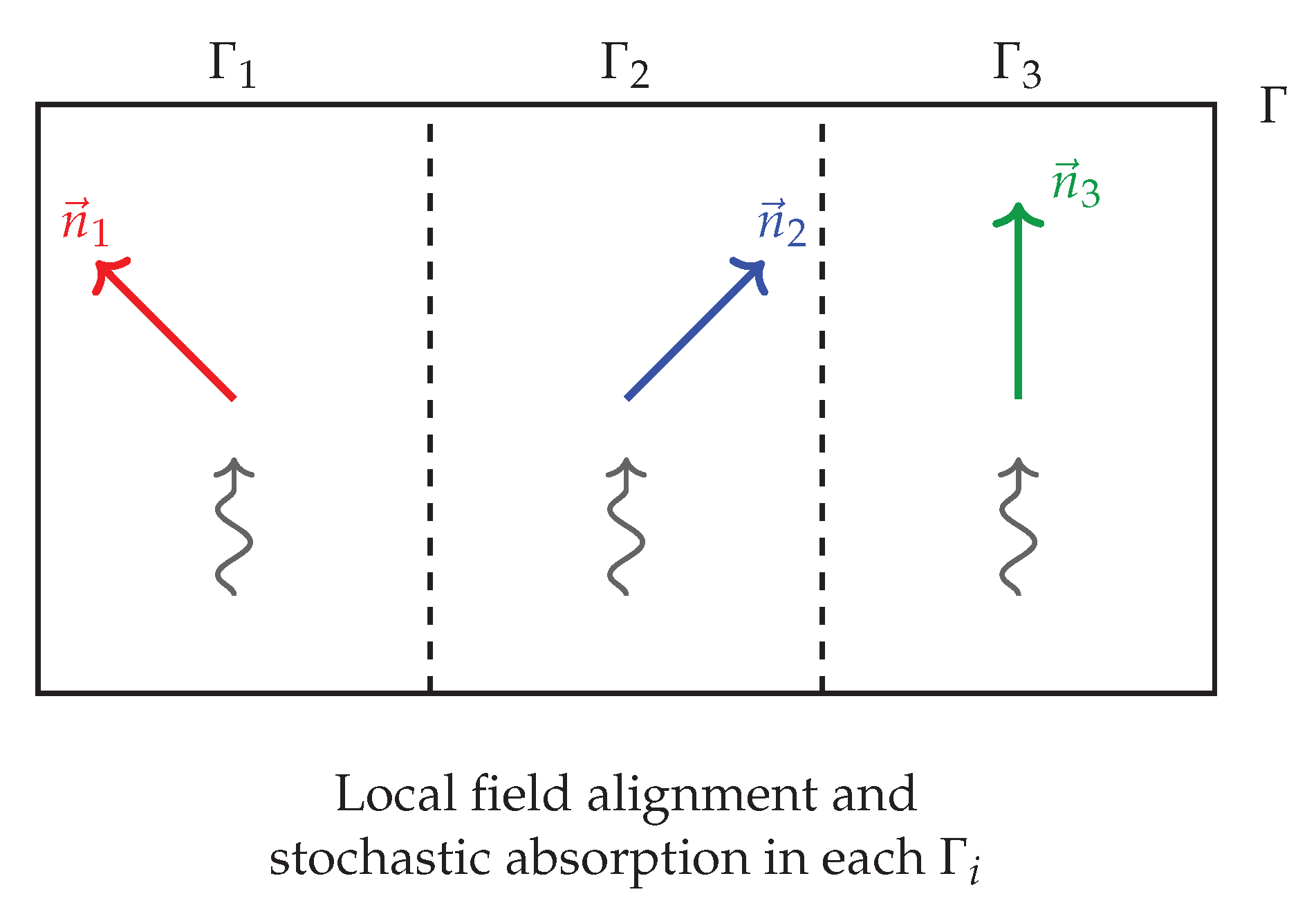
Remark A28.
See Figure A3. When the microsystem undergoes stochastic absorption within one of the eigen–domains—say, —this domain becomes the site of measurement registration, establishing a definite alignment with the corresponding apparatus direction . The remaining domains and , though still present as structural components of the apparatus interface, become dynamically suppressed. That is, they no longer carry amplitude in the post-measurement state and cease to participate in the entangled system–apparatus configuration. From the perspective of the variational dynamics, these domains no longer contribute to the extremal action paths and are effectively bypassed in the realized outcome. In this sense, they become dynamically empty, providing no support for further absorption events once the outcome is registered in .
Appendix M SDE on the Simplex with Absorbing Faces
We collect well–posedness, boundary classification, and basic identities for Itô diffusions on the probability simplex
with focus on the neutral (zero–drift) Wright–Fisher covariance and absorbing boundary at the vertices ; see, e.g., [31,33,54].
Generators, SDE representations, and invariance
We consider second–order operators on of the form
with the Wright–Fisher covariance
and drift tangent to , i.e. for all p. The form (A36) is canonical for neutral multi-allele Wright–Fisher limits [31,33].
Proposition A29 (SDE representation and invariance).
Well–posedness and boundary classification
Because is only positive semidefinite and degenerates at , strong well-posedness may fail globally; the right framework is the martingale problem with boundary conditions [31,86].
Definition A30 (Martingale problem with absorbing boundary).
Let be smooth functions compactly supported in the interior. A probability measure on solves the martingale problem for with absorbing boundary at vertices if and for all ,
is a –martingale, and if p is absorbed on first hitting any vertex : for all whenever ; cf. [86, Ch. 6].
Theorem M.1 (Existence and uniqueness in law).
Assume b is continuous, locally Lipschitz on , tangent (), and at most linear growth. Then for each initial law on , the martingale problem for (A35)–(A36) with absorbing vertices is well–posed: there exists a solution and it is unique in law. Moreover, the solution coincides with the weak solution of the SDE (A37), absorbed at the vertices [31,86].
Remark A31 (Reflecting vs. absorbing faces; mutation drift).
Conservation, martingales, and absorption times
Proposition A32 (Conservation laws and coordinate martingales).
For the neutral case :
- 1.
- for all t.
- 2.
- Each coordinate is a bounded martingale up to the absorption time , hence and [31].
Theorem M.2 (Absorption in finite time; estimates).
In the neutral, absorbing case , the first hitting time τ of the vertex set is a.s. finite with . Moreover, there exist depending only on m such that
For ,
Reflecting faces and stationary Dirichlet laws
Notes on strong solutions and pathwise uniqueness
The diffusion coefficient in (A37) is only Hölder and vanishes at , so global pathwise uniqueness need not hold; cf. the Yamada–Watanabe criteria [95]. On each compact subset of coefficients are locally Lipschitz, yielding strong well–posedness up to the (random) hitting time of the boundary [53, §5.2]. For our purposes, uniqueness in law via the martingale problem (Theorem M.1) suffices [86].
Summary and comparison
- Our main text uses the neutral, absorbing case to represent selection of a unique outcome by fixation at a vertex, with absorption probabilities given by initial coordinates (martingale/optional stopping) [31].
Appendix N Optional Stopping: Uniform Integrability and Hitting Times
This appendix states the uniform–integrability (UI) criteria and a version of Doob’s optional stopping theorem used in Section 4, and supplies complete proofs of Proposition 17, Theorem 4.1, and Lemma 18 for the Wright–Fisher diffusion on the simplex with absorbing vertices (Appendix M). Standard background can be found in [26,53,81,93].
Uniform integrability and optional stopping
Definition A34 (Uniform integrability).
A family is uniformly integrable if
A càdlàg martingale is uniformly integrable if is UI [81, §III.3].
Lemma A35 (Bounded martingales are UI).
If is a martingale with almost surely for all t, then is uniformly integrable [93, Prop. 10.10].
Proof.
For any , . Hence the defining supremum is 0 for all . □
Theorem N.1 (Doob’s optional stopping for UI martingales).
Proof of Proposition 17 (martingale property)
Recall the generator on the simplex interior (Appendix M)
with by detailed balance/symmetry (Section 4.1).
Proof of Proposition 17.
For the coordinate function , we have , , hence on . Dynkin’s formula (e.g. [53, Prop. 5.3.4]) yields that is a local martingale up to the absorption time . Because , is bounded, thus a true martingale (Lemma A35) and uniformly integrable. Therefore for all . □
Proof of Theorem 4.1 (Born probabilities by optional stopping)
Proof of Theorem 4.1.
Let be the absorption time (finite a.s. by Lemma 18). By Proposition 17, is a bounded martingale and hence uniformly integrable (Lemma A35). Applying Theorem N.1 with gives
At time , is a vertex so , i.e. . Therefore
which equals under the identification of initial overlaps with squared amplitudes in the apparatus basis. □
Proof of Lemma 18 (finite a.s. absorption and )
We provide explicit Lyapunov–function estimates on the neutral Wright–Fisher diffusion () with absorbing vertices.
Upper bound via entropy.
Let (extend continuously at the boundary by as ). For , and . Thus
a strictly negative constant on . Let . Dynkin’s formula gives
hence, letting and using with at absorption,
This proves .
Lower bound via quadratic variance.
Let . Then , so
Dynkin’s formula at yields
Letting and using ,
Since on , (A42) implies
Combining (A41)–(A43) yields finite mean absorption time with dimension–dependent bounds; for , the exact mean follows from the scale–speed calculation for one–dimensional Wright–Fisher diffusions [33, §4.6]; see also [54, §15].
Remarks on stopping at unbounded times
Summary
- Each coordinate is a bounded martingale up to absorption (Proposition 17); hence it is uniformly integrable (Lemma A35).
Appendix O Hydrodynamic Limit: Tightness and Martingale Problem
We give a complete proof of the diffusion limit stated in Theorem 3.1 and Theorem 6.1. All processes live on the compact metric state space ; hence tightness is established in the Skorokhod topology on [8,50].1
Prelimit semimartingale structure
Recall the diffusively rescaled overlap process with coordinates , cf. (17). From the microscopic dynamics (15)–(16) and Itô’s formula (ratio rule), one obtains for each i
where is an –valued continuous martingale with predictable quadratic covariation
The processes and are progressively measurable functionals of the boundary layer configuration, uniformly bounded on compacts by Assumptions 14 and 19.
Compact containment and modulus of continuity
Lemma A36 (Compact containment).
For every and there exists a compact such that
Proof.
itself is compact; hence take . The claim is tautological. □
Lemma A37 (Aldous modulus criterion).
Fix . For each ,
Proof.
Proposition A38.
Tightness in . The laws of are tight on under the Skorokhod topology.
Proof.
Remark on criterion.
If one worked with piecewise–constant channel counts (càdlàg with jumps from microscopic discretization), an criterion can be used: compact containment as above plus control of the oscillation functional on small intervals; see [92, Ch. 12].
Identification of the limit generator
Lemma A39 (Averaging of characteristics).
Under Assumptions 19(C1)–(C3), the fast boundary layer is ergodic at fixed p with reversible invariant law given by the Gibbs measure conditioned on the overlap. Then, for every ,
with
where a and are given by the Green–Kubo and drift averages (20)–(21).
Proof sketch.
By time–scale separation, decompose any observable into its conditional expectation given and a centered fluctuation. Reversibility and a spectral gap yield integrable autocovariances; consequently, the Kipnis–Varadhan theory identifies the covariance limit with the Green–Kubo integral [56]. Convergence of characteristics follows from the perturbed test function/martingale–problem method for two–time–scale Markov processes [31,61]. Detailed balance and channel symmetry force . □
Proposition A40 (Limit martingale problem).
Let along a subsequence. Then for every ,
i.e. p solves the martingale problem for with absorption at the vertices.
Proof.
From (A47) and Lemma A39,
with . Tightness and the Skorokhod representation theorem [8] yield a.s. convergence along a further subsequence; passing to the limit in the martingale identity gives the claim. Absorption is inherited from the prelimit since once a single channel carries all boundary weight, cross–channel covariations vanish; this stability is closed under weak convergence [80]. □
Lemma A41 (Uniqueness for the limit martingale problem).
The martingale problem for with covariance and absorbing vertices is well–posed (unique in law).
Proof.
See Theorem M.1 in Appendix M; cf. [31, Chs. 8–9]. □
Theorem O.1 (Hydrodynamic limit).
The family converges in distribution on to the unique solution of the martingale problem for , i.e. to the Wright–Fisher diffusion with covariance (12) and zero drift, with absorbing vertices.
Quantitative estimates and rates (sketch)
Under the spectral gap and mixing time in Assumption 19, the corrector solving the Poisson equation for the fast dynamics admits . Perturbed test function estimates then yield for and ,
consistent with the heuristic rate quoted in Section 6.2; see [78, Chs. 3–5] for quantitative averaging bounds and corrector estimates in reversible settings, and [60] for weak convergence of stochastic integrals used in diffusion approximations.
Summary
- Prelimit overlap processes are continuous semimartingales with uniformly controlled characteristics.
Appendix P Boundary Fluctuation–Dissipation and Drift Cancellation
We justify rigorously that the effective drift of the overlap diffusion on the outcome simplex vanishes under detailed balance and channel symmetry, and quantify perturbative corrections when these conditions are weakly broken.
Reversible Boundary Dynamics and Dirichlet form
Recall the overdamped, reversible boundary dynamics (8)–(9) driven by the alignment functional in (1). Let denote the generator on functionals ; by Assumption 13 it is self–adjoint on with carré du champ (Dirichlet form) [2,35]
Let the channel strengths and overlaps be defined by (17) (continuum version uses surface integrals over ). Write and .
Symmetry and Conditional Expectations
We work with the –algebra generated by the overlaps. Let denote conditional expectation under . Channel symmetry is expressed by the invariance of the microscopic model under permutations of the channel partition :
with the same strictly increasing f used in all . Then, for any bounded measurable H,
In particular, the conditional expectations of the linear and quadratic characteristics are exchangeable:
for some bounded measurable scalars depending only on p.
Drift Cancellation
Define the effective drift of p as the conditional expectation (at the micro timescale)
The drift of the macroscopic limit is then obtained from by averaging in time (Section 3); equality of the two holds already at the level of conditional expectations under time–scale separation [61,78].
Theorem P.1 (Drift cancellation).
Assume detailed balance (self–adjoint in ) and channel symmetry (A52). Then for all ,
Consequently, the limiting overlap diffusion on has zero drift: .
Proof.
Apply (A50) with and take :
Insert (A51), use (A54), and . For the first sum,
For the second sum, separate diagonal and off–diagonal parts via (A54) and compute the finite sums explicitly, obtaining
Fluctuation–dissipation (same mobility prefactors in and for reversible diffusions) and reversibility imply a Green–Kubo identity for T [42,56,78]:
Substituting cancels both and contributions, yielding . □
Remark A42 (Free–energy viewpoint).
Let be the constrained partition function (microcanonical conditional measure) at fixed p, and the corresponding constrained free energy. Under quasi–equilibrium reduction of reversible diffusions (Mori–Zwanzig/GENERIC), the slow drift takes gradient form with mobility D given by a Green–Kubo covariance [44,67,72,78,100]. Channel symmetry forces to be constant on , hence .
Conditions and Counterexamples
The cancellation in Theorem P.1 hinges on two ingredients:
- Reversibility (detailed balance): self–adjoint in and fluctuation–dissipation for bulk and boundary noise (Assumption 13); see, e.g., [35, Ch. 1].
- Channel symmetry: invariance (A52), equal channel areas, identical weights f, and channel–independent mobilities on .
Violations yield nonzero drift:
- 1.
- 2.
- 3.
- Channel–dependent f: Using different in biases the projection and again yields a nonzero ; cf. linear-response interpretation below [42].
Perturbative Corrections and Bounds
We quantify drift when symmetry is weakly broken by a small parameter (e.g. relative area/mobility mismatch , or weak nonreversible perturbation of the generator).
Proposition A43 (Linear response of the drift).
Suppose where is reversible and symmetric under (A52), and is a bounded perturbation (not necessarily symmetric). Let be the effective drift and the covariance of the projected diffusion. Then, uniformly on compact subsets of ,
where is the symmetric Wright–Fisher covariance and
is the first–order change in constrained free energy ( the constrained partition function at fixed p under ). In particular, with C depending on bounds for and mixing constants of the boundary layer [42,58,78].
Proof sketch.
Use quasi–equilibrium projection for reversible diffusions: to first order, the slow dynamics is a gradient flow of the constrained free energy with mobility (Green–Kubo), and the –dependence of is given by the logarithmic derivative of the constrained partition function (linear response) [42,78]. Mixing of the fast variables controls the response norm uniformly [58]. □
Corollary A44 (Quantitative cancellation).
Under the weak–asymmetry regime of Proposition A43, the deviation from neutral drift satisfies
where quantifies channel area/shape mismatch, mobility/noise imbalance, and the size of the skew–adjoint perturbation. This is consistent with the robustness bound in Theorem 8.1; see also [78].
Summary.
Detailed balance fixes the relation between drift and noise (fluctuation–dissipation). Permutation symmetry forces the constrained free energy to be constant on , hence the projected drift vanishes identically. Small violations introduce a drift that is the gradient of an effective free energy and is perturbatively small, with size controlled by symmetry–breaking and nonreversibility parameters.
Appendix Q Sanov and Varadhan Tools
This appendix states the large–deviation inputs used in Section 7 and records short proofs tailored to a finite outcome alphabet . We write for the set of laws on . For a sequence of outcomes with one–trial law , the empirical measure (frequency vector) is
Sanov’s theorem on a finite alphabet
Theorem Q.1 (Sanov, finite alphabet).
Let be i.i.d. with . Then satisfies an LDP on with speed N and good, convex rate function
with the convention and if for some i with .
Proof sketch.
Theorem Q.2 (Sanov under –mixing).
Assume is strictly stationary with one–trial law and α–mixing coefficients satisfying for some . Then obeys the same LDP as in Theorem Q.1 with rate .
Proof sketch.
Partition into big blocks of size separated by gaps of size with , , and . By mixing, blocks are asymptotically independent in the exponential scale; apply Sanov on blocks and control the contribution of gaps (negligible in the speed N). Equivalently, use the Gärtner–Ellis theorem: the log–MGF of admits the same limit by block decoupling. See [19, §4.5] and [71]. □
Varadhan’s lemma and the convex dual I
Let and define the scaled cumulant generating function (SCGF)
whenever the limit exists and is finite on all .
Lemma A45 (SCGF for i.i.d. and mixing sequences).
Proof.
Theorem Q.3 (Varadhan/Gärtner–Ellis).
Suppose Λ exists, is lower semicontinuous and essentially smooth on (true for (A57)). Then satisfies an LDP with good, convex rate function given by the Legendre–Fenchel transform
Proof.
Proposition A46 (Identification of I as relative entropy).
Application to Theorem 7.1 and Proposition 23
Theorem 7.1.
Part (i) is Theorem Q.1. Part (ii) follows from Theorem Q.2, which in turn can be derived via Theorem Q.3 using Lemma A45.
Proposition 23.
Let denote the tilted partition function of N windows (or trials). Assumption 22(F1) asserts uniformly on compacts, and (F2) gives exponential tightness of under the tilted laws. Applying Varadhan’s lemma (or Gärtner–Ellis) yields the LDP with rate I given by (A58), which equals by Proposition A46.
Remarks
- Goodness of I. On the compact set , I has compact level sets automatically.
- Zeros in . If for some i, then unless . This matches the fact that outcomes with zero single–trial probability almost surely never appear in the empirical measure.
- Contraction. Any continuous linear map of (e.g. binning degenerate outcomes) inherits the LDP with the contracted rate; grouping coordinates gives [19, §4.2].
Appendix R Notation and Glossary
This appendix collects the principal symbols, objects, and standing assumptions used throughout.
Sets, geometry, and indices
- m
- Number of measurement channels (outcomes), .
- Probability simplex .
- ith vertex of (unit vector with 1 in coordinate i).
- Foliation leaf (intrinsic time slice) induced by the stabilized apparatus field .
- Interface (detector) boundary on , partitioned into channel domains .
- Euclidean pairing on (for vectors of channel weights).
- Indices
- Roman denote channel coordinates.
Chronon fields, coarse–graining, and energies
- Microscopic chronon vector field (fine scale).
- Coarse–grained (effective) chronon field; denotes the stabilized apparatus field (unit–norm, twist–free on ).
- Alignment free energy with interface penalty ; in discrete form generates .
- Microscopic energy on the boundary layer lattice; includes nearest–neighbor couplings, norm pinning, and boundary alignment with strength .
- Inverse temperature in Gibbs measures (thermal noise parameter).
- Gibbs measure on the boundary layer associated with (or ), reversible for the microscopic dynamics.
- f
- Fixed strictly increasing scalar function used to build channel strengths from local alignments (e.g. ).
Channel strengths, overlaps, and observables
- Channel strength for : boundary integral (continuum) or sum (discrete) of f applied to the local alignment with .
- T
- Total strength .
- Normalized overlap , .
- Initial overlap vector for a prepared microdomain on the interface.
Stochastic dynamics and generators
- Generator of the reversible microscopic (boundary) diffusion for ; self–adjoint in .
- Carré du champ ; Dirichlet form .
- Overlap process on (projected slow variable).
- Diffusion intensity of the overlap process; Green–Kubo coefficient extracted from boundary fluctuations.
- Covariance matrix on : (Wright–Fisher form).
- Effective drift on (vanishes under detailed balance and channel symmetry).
- Limit generator on : .
- Absorption (fixation) time: .
Hydrodynamic scaling and prelimit objects
- Microscopic lattice spacing (ultraviolet scale).
- Coarse–graining (mesoscopic) block scale; in the limit.
- Boundary layer neighborhood of of thickness .
- Diffusively rescaled prelimit overlap process (time scale ).
- Prelimit semimartingale characteristics of (drift and quadratic covariation).
Large deviations and thermodynamic tilts
- Empirical frequency vector from N repeated trials: .
- Sanov rate function on .
- Limiting scaled cumulant generating function: .
- Tilted partition function for N windows/trials: .
Standing assumptions (cross–reference)
- Assumption 16
- Regularity and symmetry of the limit SDE: Lipschitz coefficients on , nonexplosion, absorbing faces, and channel permutation symmetry (implies zero drift).
- Assumption 19
- Mixing/propagation of chaos for the boundary layer: spectral gap, exponential decorrelation on scale , and fast mixing compared to diffusive scaling.
- Assumption 13
- Detailed balance and fluctuation–dissipation: reversible in and noise consistent with thermal equilibrium.
- Assumption 14
- Well–posedness of the microscopic SPDE/SDE with boundary conditions induced by ; existence of the Gibbs invariant measure.
- Assumption 22
- Approximate factorization for repeated windows/trials: additivity of free energy and exponential tightness for tilted measures (used in Varadhan derivation).
Frequently used functions and inequalities
- Shannon entropy ; controls mean fixation times (Appendix M).
- Quadratic variance ; Lyapunov function for absorption (Appendix M).
- Kullback–Leibler divergence (relative entropy).
- BDG
- Burkholder–Davis–Gundy inequalities for martingale increments (tightness).
- Aldous
- Aldous–Rebolledo tightness criterion for semimartingales on .
Typographic Conventions
- ,
- Deterministic and stochastic differentials in Itô form.
- ,
- First and second partial derivatives with respect to .
- ⇒
- Convergence in distribution (weak convergence) on Skorokhod space.
- ≍
- Asymptotic proportionality up to dimensionless constants depending on fixed parameters (geometry, stiffness).
Appendix P: A Pedagogical Guide to the Derivation
P.0 Narrative Overview: From Field Alignment to Born Probabilities
This appendix provides a pedagogical overview of the derivation of the Born rule in Chronon Field Theory (ChFT), with an emphasis on the key ideas, probabilistic tools, and logical flow. Readers may wish to begin with this section to orient themselves before working through the formal results in detail.
Initial Setup and Physical Picture.
The measurement process in CFT begins with a microscopic chronon field loosely aligned across a boundary interface with a macroscopic apparatus field . The apparatus is pre-aligned with a fixed future-directed, unit-norm, twist-free configuration, and the interface is partitioned into m disjoint channels corresponding to possible outcomes. The local alignment between and across each channel determines a scalar score , which is then normalized to yield a probability-like overlap coordinate:
This defines the initial vector , the outcome simplex, which encodes how strongly the chronon field initially aligns with each outcome channel.
Why matters.
The initial overlaps play the role of effective amplitude squares . They capture all physically accessible information about the prepared state relevant to measurement outcomes, in a manner consistent with the apparatus geometry and coarse–graining; they serve as the initial condition for the stochastic process , whose evolution determines the measurement result. Conceptually, this highlights a shift from the textbook picture: the measurement is not a collapse of the system into one of its own eigenstates, but stochastic absorption of the system field into apparatus eigen–domains. Since apparatus domains are engineered to correspond to the system’s eigenbasis, there is no contradiction with the standard account; rather, CFT provides a deeper dynamical explanation of why those eigenstates appear as possible outcomes.
From Stochastic Dynamics to Absorption.
The dynamics of arises from a noisy alignment process—specifically, a stochastic gradient flow for coupled to the apparatus across . Under a hydrodynamic scaling limit, this yields a diffusion process on governed by a neutral (zero-drift) Wright–Fisher-type stochastic differential equation. This process has the following properties:
- It starts at ;
- Each coordinate is a bounded martingale;
- The process is almost surely absorbed at one of the vertices (i.e., for some i);
- Absorption is irreversible and corresponds to a definite measurement outcome.
Deriving the Born Rule.
Since each is a martingale up to the absorption time , the optional stopping theorem applies:
But is the indicator function for outcome i, so this expectation is exactly the probability of observing i:
Thus, the Born rule emerges.
P.1 What the Born Rule Says (and How We Will Phrase It)
Statement. If a system is prepared in state and measured in an orthonormal basis , the probability of outcome is
Interface phrasing. In our setup, the apparatus interface is partitioned into m disjoint channels (distinct pointer regions). We form alignment overlaps that sum to 1, so the vector lies on the outcome simplex
The target is to show that single–shot outcome probabilities equal the initial overlaps:
Illustration: See Figure A4, diagram of the simplex for with a point and absorbing vertices:
Figure A4.
Simplex for . Vertices are absorbing; (red) marks an initial overlap vector. Dotted guides indicate barycentric geometry; faint arrows suggest possible neutral diffusion paths toward vertices.
Figure A4.
Simplex for . Vertices are absorbing; (red) marks an initial overlap vector. Dotted guides indicate barycentric geometry; faint arrows suggest possible neutral diffusion paths toward vertices.
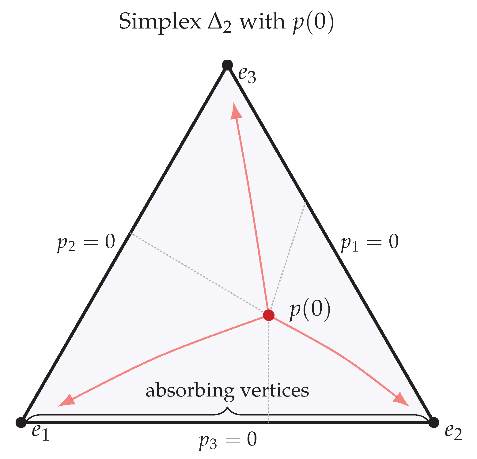
P.2 Why Derive It Rather Than Assume It?
- Foundational clarity. We seek a dynamics–based route to probabilities, avoiding postulates.
- Device–level parameters. The diffusion intensity and timescales are tied to measurable interface properties (coupling, temperature).
- Robustness. Small asymmetries or imperfections appear as small drifts/covariance perturbations whose effects can be bounded.
High–level roadmap. (i) boundary alignment ⇒ stochastic overlap dynamics on ; (ii) under symmetry and detailed balance, each coordinate has zero drift (is a martingale); (iii) absorption at vertices gives outcome probabilities by optional stopping.
P.3 Chronons, overlaps, and noise: the physical picture
Chronon alignment. A microscopic field in a boundary layer near tends to align with the stabilized apparatus field. Thermal/environmental noise at the boundary shakes this alignment.
- Overlaps . Spatially averaged alignment “strengths’’ over each channel , normalized to sum to 1.
- Neutral fluctuations. With symmetric channels and detailed balance, fluctuations are unbiased among channels: no preferred direction on .
- Absorption. Once one channel dominates (all weight at a vertex of ), the process is effectively locked in: a definite outcome.
Therefore, the coarse–grained dynamics is a neutral diffusion on with absorbing vertices.
In the following Illustration, Figure A5, the boundary layer of the apparatus region interface splits into channels, with arrows showing alignment and noise:
Figure A5.
Boundary layer. The microdomain (left) aligns with the apparatus field in A (right) through the interface , which is partitioned into channels . Solid green arrows indicate alignment flow across the interface; wavy red arrows depict boundary noise. Bars on the apparatus side schematically represent overlap observables .
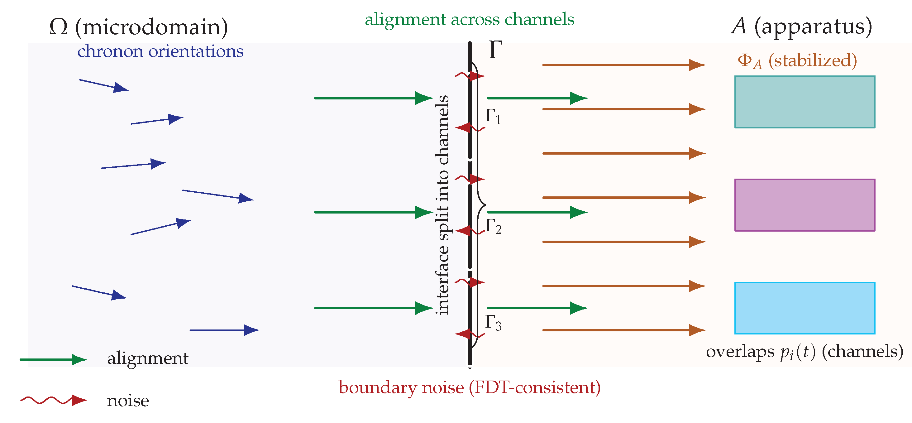
P.4 The two–outcome case (): martingale ⇒ Born probabilities
Let and write for the weight of channel 1 (so channel 2 has ). The neutral diffusion on the 1–simplex takes the canonical form
where is a diffusion intensity set by boundary fluctuations and is standard Brownian motion.
Key facts (intuition, no heavy measure theory needed).
- 1.
- Martingale property. Since there is no drift term in (A61), the conditional expectation stays constant:
- 2.
- Absorption (fixation). The endpoints are absorbing; with probability 1, hits in finite time (no “hovering’’ forever in the open interval).
- 3.
-
Optional stopping. Let be the first hitting time of . For bounded martingales like , the optional stopping theorem givesBut , so .
Conclusion (two–outcome Born rule).
Identifying matches the Born rule.
Illustration: 1D sketch of as a random path starting at and hitting 0 or 1 (See Figure A6):
Figure A6.
One-dimensional sketch of the overlap coordinate under neutral diffusion. The process starts at (red) and, depending on noise, is absorbed at (solid path, time ) or at (dashed path, time ).
Figure A6.
One-dimensional sketch of the overlap coordinate under neutral diffusion. The process starts at (red) and, depending on noise, is absorbed at (solid path, time ) or at (dashed path, time ).
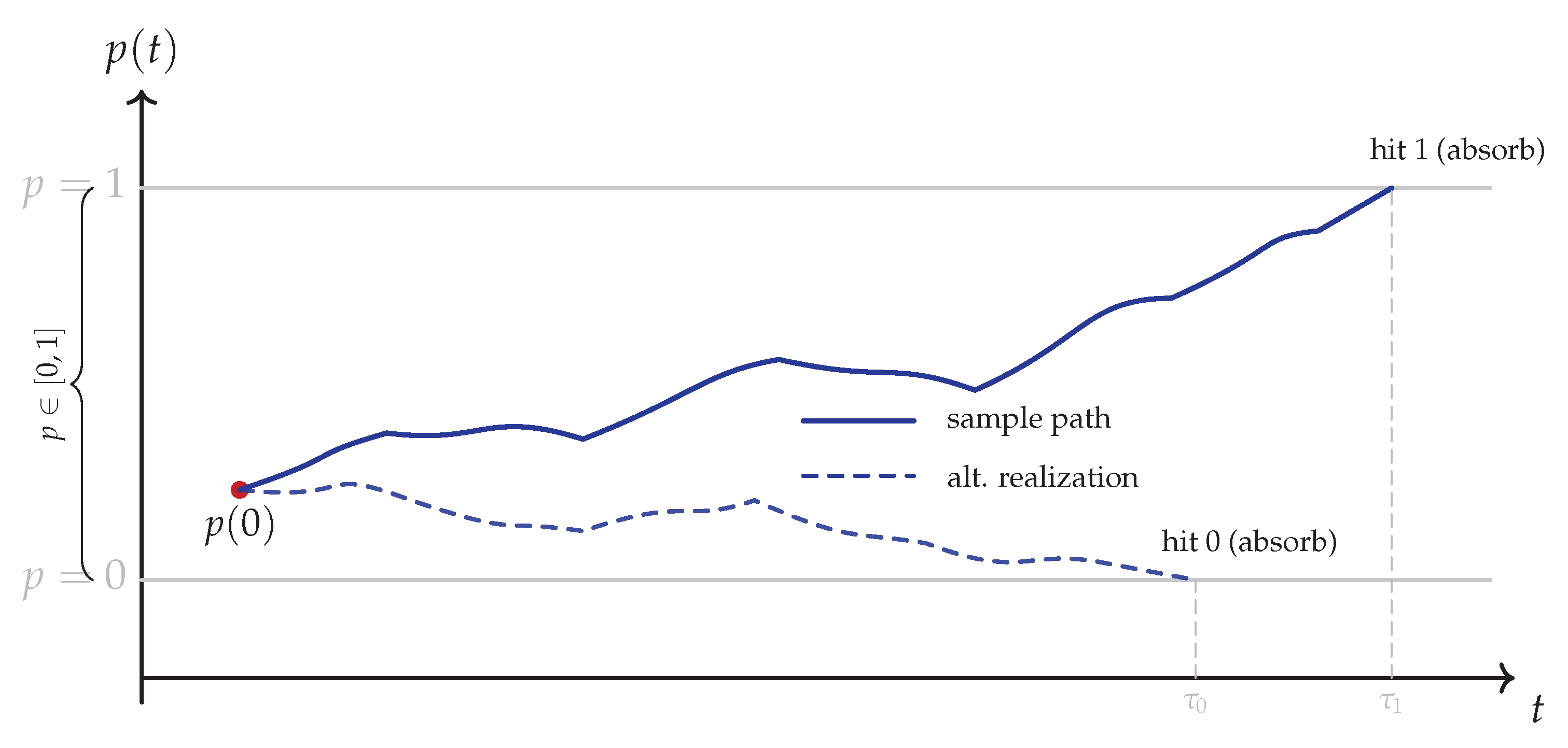
P.5 From Two Outcomes to Many: Simplex Diffusion, Frequencies, and Robustness
Many outcomes. For , the overlap vector follows a neutral Wright–Fisher diffusion:
with absorbing vertices (pure channels). Each coordinate is a bounded martingale, so the same optional–stopping logic gives
Repeated trials & frequencies. Independent repeats (or sufficiently mixing repeats) produce empirical frequencies that concentrate at with exponentially small tails; the large–deviation rate is the relative entropy .
Robustness. Small asymmetries or finite–temperature effects appear as a small drift or a small perturbation of the covariance. Deviations in absorption probabilities can be bounded proportionally to these small parameters (qualitative statement).
Illustration: 2D simplex () with sample diffusion paths from to vertices (See Figure A7):
Figure A7.
Diffusion on the simplex starting at (red). Sample paths (colored) terminate at absorbing vertices , illustrating fixation to a single outcome.
Figure A7.
Diffusion on the simplex starting at (red). Sample paths (colored) terminate at absorbing vertices , illustrating fixation to a single outcome.
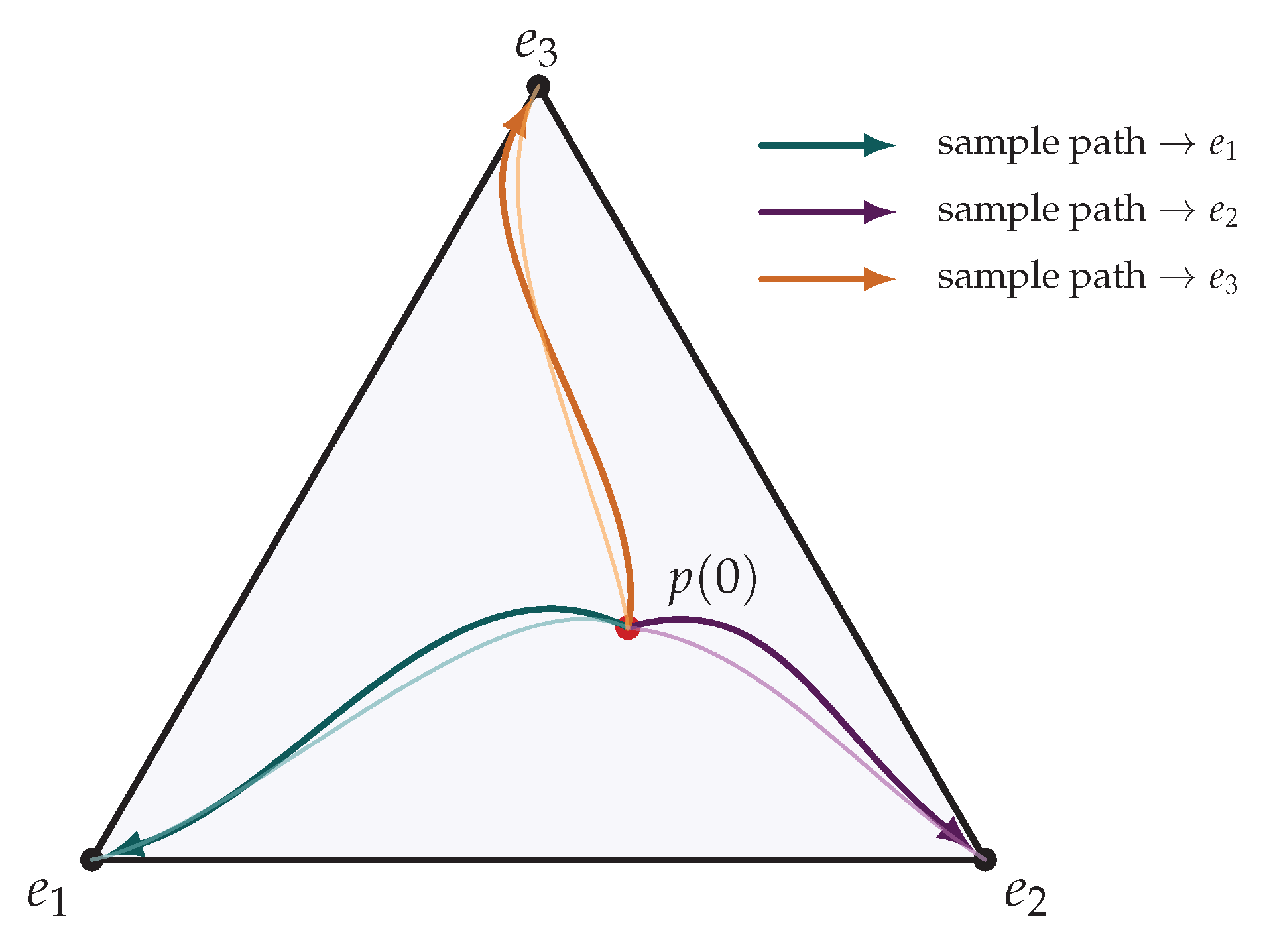
P.6 Martingales and Optional Stopping
A stochastic process adapted to a filtration is called a martingale if
and . Intuitively, martingales have no drift: their conditional expectation at a later time is the current value.
A key tool in our derivation is the optional stopping theorem (OST), which provides conditions under which for a random stopping time . For bounded martingales, OST holds for any bounded stopping time. In our context, the coordinate processes on the simplex are martingales that almost surely hit one of the absorbing vertices. OST then identifies the absorption probabilities with the initial values . See Figure A8 for an illustration.
Figure A8.
A martingale path (blue) stopped at a random time . Optional stopping ensures .
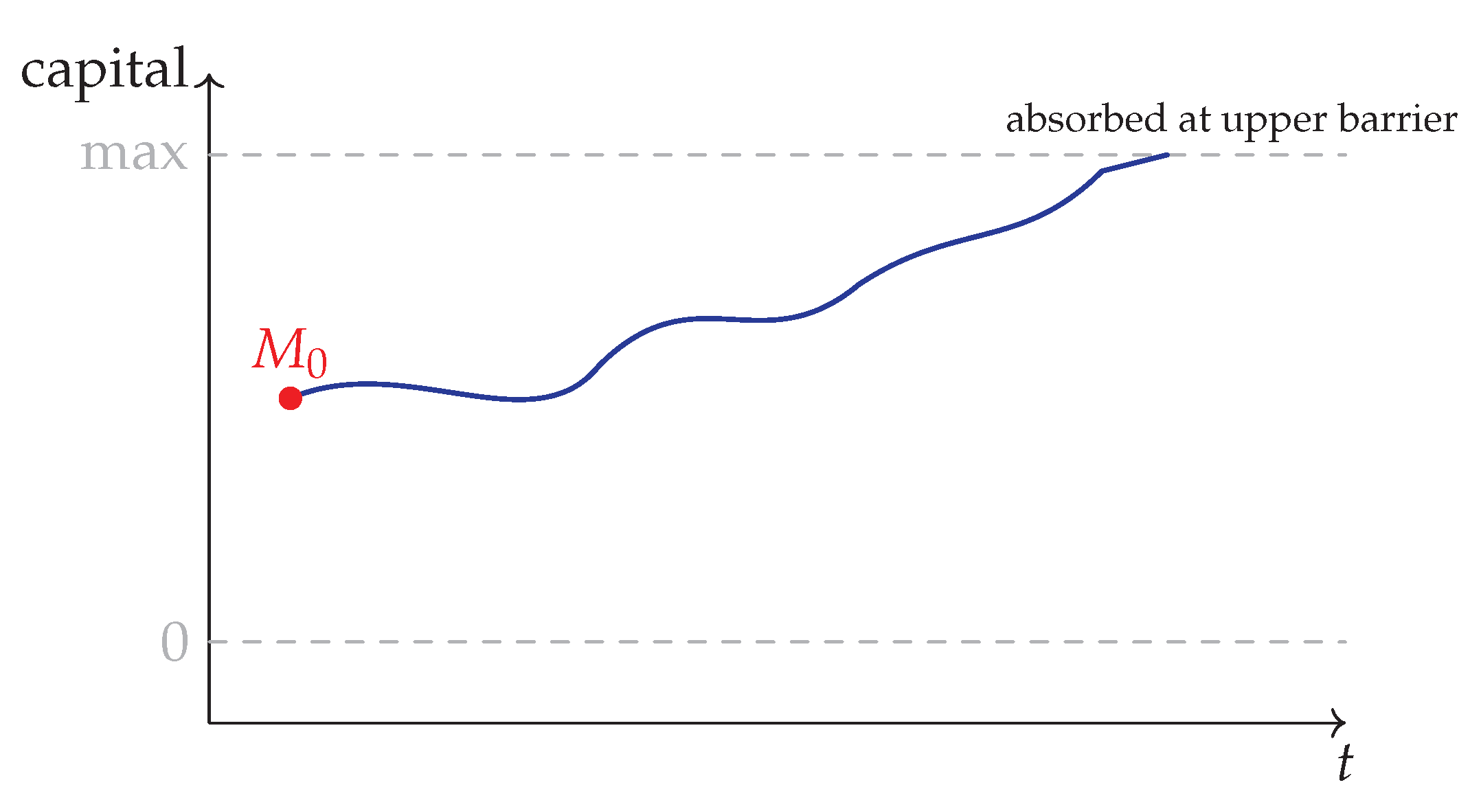
P.7 Wright–Fisher Diffusions on the Simplex
The Wright–Fisher diffusion is a canonical stochastic model for allele frequencies in a population of fixed size. For m types, the state space is the simplex
In the diffusion limit of large populations, the process evolves according to the Itô SDE
with correlated Brownian motions . The vertices of are absorbing: once the process hits a vertex (fixation of a single type), it remains there. The absorption probabilities equal the initial proportions, echoing the martingale property.
In our apparatus model, the overlap coordinates follow an analogous diffusion with absorbing vertices, making the Wright–Fisher process a natural reference point. See Figure A9 for an illustration.
Figure A9.
Wright–Fisher diffusion on : starting from , sample paths eventually fixate at one absorbing vertex.
Figure A9.
Wright–Fisher diffusion on : starting from , sample paths eventually fixate at one absorbing vertex.
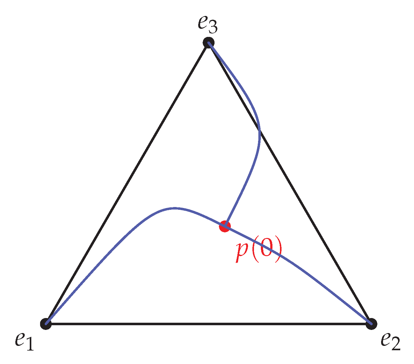
P.8 Relative Entropy and Sanov’s Theorem
Relative entropy (or Kullback–Leibler divergence) between two probability distributions q and p on a finite alphabet is
It is always nonnegative and vanishes iff .
Sanov’s theorem describes the large deviations of empirical measures from i.i.d. samples. If are drawn i.i.d. from distribution p, and denotes the empirical distribution, then
in the sense of large-deviation asymptotics. Thus the most likely empirical frequency vector is p itself, and deviations are exponentially suppressed with rate .
In our repeated-trial setting, Sanov’s theorem explains why the empirical frequencies of outcomes concentrate near the Born vector, with relative entropy furnishing the rate function of the large-deviation principle. See Figure A10 for an illustration.
Figure A10.
Sanov’s theorem: the probability that empirical frequencies (red) deviate from the true distribution (blue) decays like .
Figure A10.
Sanov’s theorem: the probability that empirical frequencies (red) deviate from the true distribution (blue) decays like .
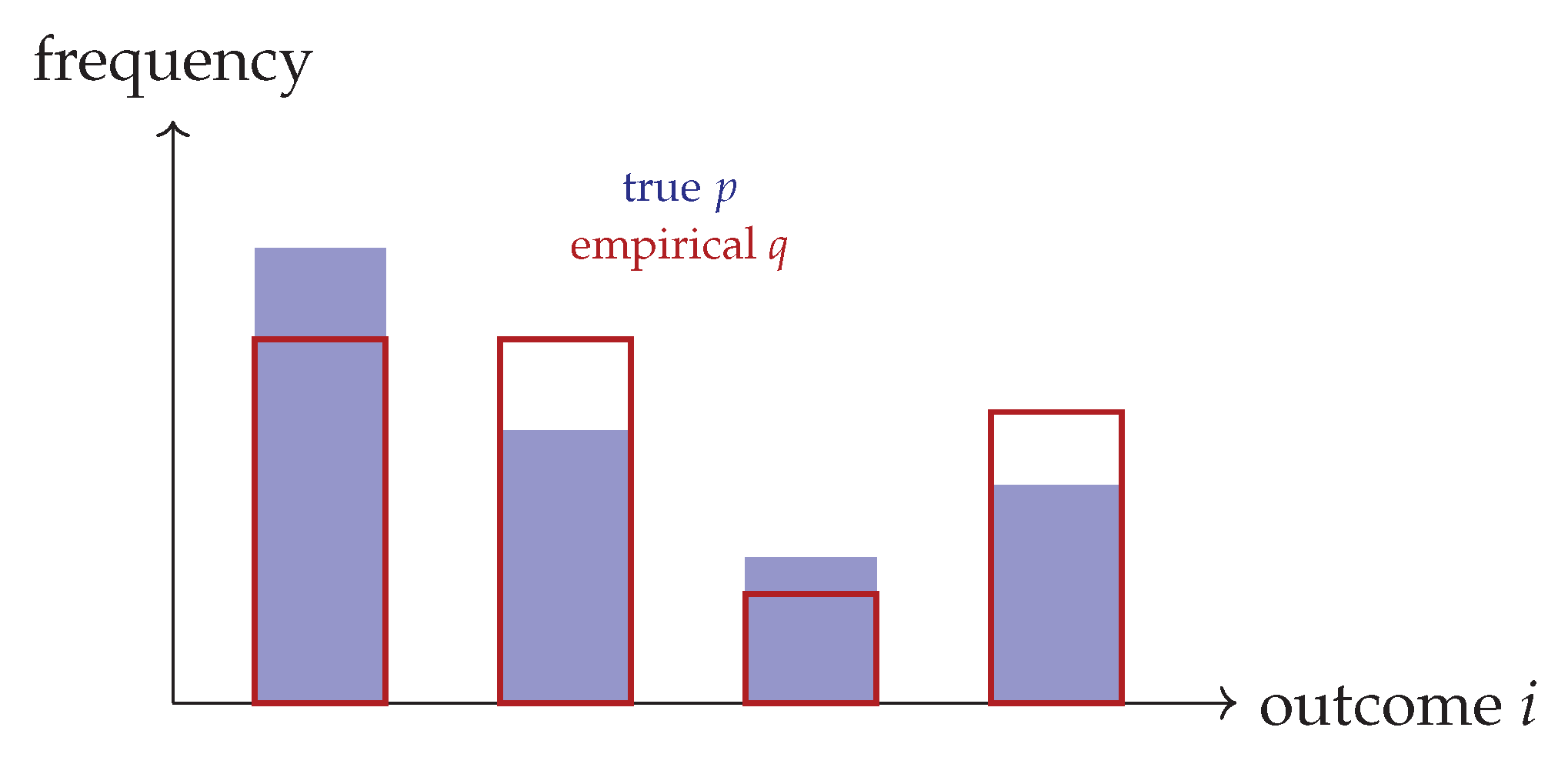
Funding
This research received no external funding
Abbreviations
The following abbreviations are used in this manuscript:
| ChFT | Chronon Field Theory |
References
- D. J. Aldous. Stopping times and tightness. Annals of Probability, 6(2):335–340, 1978. [CrossRef]
- D. Bakry, I. Gentil, and M. Ledoux. Analysis and Geometry of Markov Diffusion Operators. Springer, 2014.
- A. Barchielli and M. Gregoratti. Quantum Trajectories and Measurements in Continuous Time: The Diffusive Case. Springer, 2009.
- A. Bassi and G. C. Ghirardi. Dynamical reduction models. Physics Reports, 379(5-6):257–426, 2003. [CrossRef]
- A. Bassi and G. C. Ghirardi. The GRW model: Past, present and future. J. Phys. A: Math. Theor., 40:2919–2933, 2009.
- A. Bassi, K. Lochan, S. Satin, T. P. Singh, and H. Ulbricht. Models of wave-function collapse, underlying theories, and experimental tests. Rev. Mod. Phys., 85(2):471–527, 2013. [CrossRef]
- P. Billingsley. Probability and Measure, 3rd ed. Wiley, 1995.
- P. Billingsley. Convergence of Probability Measures, 2nd ed. Wiley, 1999.
- H. Brezis, Functional Analysis, Sobolev Spaces and Partial Differential Equations, Springer, 2010.
- W. Bryc and A. Dembo. Large deviations for quadratic functionals of stationary Gaussian processes. J. Theor. Probab., 9(4):725–752, 1996.
- P. Busch. Is the quantum state (an) observable? In Quantum Structures and the Nature of Reality, pp. 61–70. Springer, 1999.
- P. Busch, P. Lahti, and P. Mittelstaedt. The Quantum Theory of Measurement, 2nd ed. Springer, 1996.
- C. M. Caves, C. A. Fuchs, and R. Schack. Quantum probabilities as Bayesian probabilities. Phys. Rev. A, 65:022305, 2002. [CrossRef]
- D. Chandler. Introduction to Modern Statistical Mechanics. Oxford University Press, 1987.
- B. S. Cirel’son. Quantum generalizations of Bell’s inequality. Lett. Math. Phys., 4(2):93–100, 1980. [CrossRef]
- T. M. Cover and J. A. Thomas. Elements of Information Theory, 2nd ed. Wiley, 2006.
- G. Da Prato and J. Zabczyk. Stochastic Equations in Infinite Dimensions. Cambridge University Press, 1992.
- J. Dedecker and F. Merlevède. Necessary and sufficient conditions for the conditional central limit theorem. Annals of Probability, 34(3):1044–1051, 2006. [CrossRef]
- A. Dembo and O. Zeitouni. Large Deviations Techniques and Applications, 2nd ed. Springer, 1998.
- D. Deutsch. Quantum theory of probability and decisions. Proc. R. Soc. Lond. A, 455:3129–3137, 1999. [CrossRef]
- L. Diósi. A universal master equation for the gravitational violation of quantum mechanics. Phys. Lett. A, 120(8):377–381, 1987. [CrossRef]
- L. Diósi. Continuous quantum measurement and Itô formalism. Phys. Lett. A, 129(8-9):419–423, 1988. [CrossRef]
- R. L. Dobrushin. The description of a random field by means of conditional probabilities and conditions of its regularity. Theory of Probability and Its Applications, 13(2):197–224, 1968. [CrossRef]
- H.-O. Georgii. Gibbs Measures and Phase Transitions, 2nd ed. de Gruyter, 2011.
- F. den Hollander. Large Deviations. American Mathematical Society, 2000.
- J. L. Doob. Stochastic Processes. Wiley, 1953.
- R. Durrett. Probability Models for DNA Sequence Evolution, 2nd ed. Springer, 2008.
- R. Durrett. Probability: Theory and Examples, 5th ed. Cambridge University Press, 2019.
- R. S. Ellis. Entropy, Large Deviations, and Statistical Mechanics. Springer, 1985.
- C. L. Epstein and R. Mazzeo. Wright–Fisher diffusion in one dimension. SIAM J. Math. Anal., 45(2):625–652, 2013.
- S. N. Ethier and T. G. Kurtz. Markov Processes: Characterization and Convergence. Wiley, 1986.
- L. C. Evans, Partial Differential Equations, 2nd ed., Graduate Studies in Mathematics, Vol. 19, American Mathematical Society, 2010.
- W. J. Ewens. Mathematical Population Genetics I: Theoretical Introduction, 2nd ed. Springer, 2004.
- C. A. Fuchs, N. D. Mermin, and R. Schack. An introduction to QBism with an application to the locality of quantum mechanics. Am. J. Phys., 82(8):749–754, 2014. [CrossRef]
- M. Fukushima, Y. Oshima, and M. Takeda. Dirichlet Forms and Symmetric Markov Processes, 2nd ed. de Gruyter, 2011.
- D. A. Freedman. On tail probabilities for martingales. Annals of Probability, 3(1):100–118, 1975. [CrossRef]
- M. I. Freidlin and A. D. Wentzell. Random Perturbations of Dynamical Systems, 3rd ed. Springer, 2012.
- M. Gell-Mann and J. B. Hartle. Quantum mechanics in the light of quantum cosmology. In Complexity, Entropy and the Physics of Information, 1990.
- G. C. Ghirardi, A. Rimini, and T. Weber. Unified dynamics for microscopic and macroscopic systems. Phys. Rev. D, 34(2):470–491, 1986. [CrossRef]
- N. Gisin. Quantum measurements and stochastic processes. Phys. Rev. Lett., 52:1657–1660, 1984. [CrossRef]
- A. M. Gleason. Measures on the closed subspaces of a Hilbert space. J. Math. Mech., 6(6):885–893, 1957.
- M. S. Green. Markoff random processes and the statistical mechanics of time-dependent phenomena. II. J. Chem. Phys., 22:398–413, 1954. R. Kubo. Statistical-mechanical theory of irreversible processes. I. J. Phys. Soc. Japan, 12(6):570–586, 1957. [CrossRef]
- R. C. Griffiths. The expected time to absorption in neutral stochastic processes. Advances in Applied Probability, 11(3):486–501, 1979.
- M. Grmela and H. C. Öttinger. Dynamics and thermodynamics of complex fluids. I. Physical Review E, 56(6):6620–6632, 1997. [CrossRef]
- M. Hairer, An Introduction to Stochastic PDEs, arXiv:0907.4178, 2011. [CrossRef]
- N. Harrigan and R. W. Spekkens. Einstein, incompleteness, and the epistemic view of quantum states. Found. Phys., 40:125–157, 2010. [CrossRef]
- S. W. Hawking and G. F. R. Ellis, The Large Scale Structure of Space-Time, Cambridge University Press, 1973.
- W. Hoeffding. Probability inequalities for sums of bounded random variables. J. Am. Stat. Assoc., 58(301):13–30, 1963. [CrossRef]
- R. Holley and D. Stroock. Logarithmic Sobolev inequalities and stochastic Ising models. Communications in Mathematical Physics, 115(3):553–569, 1988.
- J. Jacod and A. N. Shiryaev. Limit Theorems for Stochastic Processes, 2nd ed. Springer, 2003.
- E. Joos et al. Decoherence and the Appearance of a Classical World in Quantum Theory, 2nd ed. Springer, 2003.
- O. Kallenberg. Foundations of Modern Probability, 2nd ed. Springer, 2002.
- I. Karatzas and S. E. Shreve. Brownian Motion and Stochastic Calculus, 2nd ed. Springer, 1991.
- S. Karlin and H. M. Taylor. A Second Course in Stochastic Processes. Academic Press, 1981.
- C. Kipnis and C. Landim. Scaling Limits of Interacting Particle Systems. Springer, 1999.
- C. Kipnis and S. R. S. Varadhan. Central limit theorem for additive functionals of reversible Markov processes. Communications in Mathematical Physics, 104(1):1–19, 1986. [CrossRef]
- P. E. Kloeden and E. Platen. Numerical Solution of Stochastic Differential Equations. Springer, 1992.
- T. Komorowski, C. Landim, and S. Olla. Fluctuations in Markov Processes: Time Symmetry and Martingale Approximation. Springer, 2012.
- R. Kubo. The fluctuation–dissipation theorem. Reports on Progress in Physics, 29(1):255–284, 1966. [CrossRef]
- T. G. Kurtz and P. Protter. Weak limit theorems for stochastic integrals and stochastic differential equations. Annals of Probability, 19(3):1035–1070, 1991. [CrossRef]
- T. G. Kurtz. Averaging for martingale problems. In Stochastic Analysis, pp. 186–209. Academic Press, 1992.
- D. A. Levin and Y. Peres. Markov Chains and Mixing Times, 2nd ed. AMS, 2017.
- B. Li. Emergence and Exclusivity of Lorentzian Signature and Unit–Norm Time from Random Chronon Dynamics. Zenodo, . [CrossRef]
- R. S. Liptser and A. N. Shiryayev. Statistics of Random Processes I: General Theory. Springer, 1977.
- C. Maes and K. Netočný. Time-reversal and entropy. Journal of Statistical Physics, 110(1):269–310, 2003. [CrossRef]
- S. P. Meyn and R. L. Tweedie, Markov Chains and Stochastic Stability, 2nd ed. Cambridge University Press, 2009.
- H. Mori. Transport, collective motion, and Brownian motion. Progress of Theoretical Physics, 33(3):423–455, 1965. [CrossRef]
- M. A. Naimark. Spectral functions of a symmetric operator. Izvestiya Akad. Nauk SSSR Ser. Mat., 4:277–318, 1940.
- E. Nelson. Derivation of the Schrödinger equation from Newtonian mechanics. Phys. Rev., 150(4):1079–1085, 1966. [CrossRef]
- A. Dembo and O. Zeitouni. Large Deviations Techniques and Applications, 2nd ed. Springer, 1998.
- S. Orey and S. Pelikan. Large deviations for stationary processes. Annals of Probability, 17(4):1481–1495, 1989.
- H. C. Öttinger. Beyond Equilibrium Thermodynamics. Wiley, 2005.
- G. C. Papanicolaou and W. Kohler, Asymptotic theory of mixing stochastic ordinary differential equations, Communications on Pure and Applied Mathematics, 27(5):641–668, 1974. [CrossRef]
- G. A. Pavliotis. Stochastic Processes and Applications. Springer, 2014.
- G. A. Pavliotis and A. M. Stuart. Multiscale Methods: Averaging and Homogenization. Springer, 2008.
- R. Penrose. On gravity’s role in quantum state reduction. Gen. Relativ. Gravit., 28(5):581–600, 1996. [CrossRef]
- A. Peres. Neumark’s theorem and quantum inseparability. Foundations of Physics, 20:1441–1453, 1990. [CrossRef]
- G. A. Pavliotis and A. M. Stuart. Multiscale Methods: Averaging and Homogenization. Springer, 2008.
- R. Rebolledo. Central limit theorems for local martingales. Zeitschrift für Wahrscheinlichkeitstheorie und Verwandte Gebiete, 51:269–286, 1980. [CrossRef]
- J. Jacod and A. N. Shiryaev. Limit Theorems for Stochastic Processes, 2nd ed. Springer, 2003.
- D. Revuz and M. Yor. Continuous Martingales and Brownian Motion, 3rd ed. Springer, 1999.
- I. N. Sanov. On the probability of large deviations of random variables. Mat. Sb., 42(84):11–44, 1957.
- R. D. Skeel and J. Izaguirre. An impulse integrator for Langevin dynamics. Molecular Physics, 100(24):3885–3891, 2002. [CrossRef]
- R. W. Spekkens. Evidence for the epistemic view of quantum states: A toy theory. Phys. Rev. A, 75:032110, 2007. [CrossRef]
- H. Spohn, Large Scale Dynamics of Interacting Particles, Springer, 1991.
- D. W. Stroock and S. R. S. Varadhan, Multidimensional Diffusion Processes, Springer, 1979.
- S. R. S. Varadhan. Large Deviations and Applications. SIAM, 1984.
- S. R. S. Varadhan. Stochastic Processes. Courant Lecture Notes in Mathematics, vol. 16, AMS/CIMS, 2007.
- R. Vershynin. High-Dimensional Probability: An Introduction with Applications in Data Science. Cambridge University Press, 2018.
- J. von Neumann. Mathematical Foundations of Quantum Mechanics. Princeton University Press, 1955.
- D. Wallace. The Emergent Multiverse: Quantum Theory According to the Everett Interpretation. Oxford University Press, 2012.
- W. Whitt. Stochastic-Process Limits. Springer, 2002.
- D. Williams. Probability with Martingales. Cambridge University Press, 1991.
- H. M. Wiseman and G. J. Milburn. Quantum Measurement and Control. Cambridge University Press, 2009.
- T. Yamada and S. Watanabe. On the uniqueness of solutions of stochastic differential equations. Journal of Mathematics of Kyoto University, 11(1):155–167, 1971.
- B. Zegarliński. Logarithmic Sobolev inequalities for Gibbs measures. Probability Theory and Related Fields, 89(2):199–213, 1991.
- W. H. Zurek. Environment-induced superselection rules. Phys. Rev. D, 26(8):1862–1880, 1982. [CrossRef]
- W. H. Zurek. Decoherence, einselection, and the quantum origins of the classical. Rev. Mod. Phys., 75(3):715–775, 2003. [CrossRef]
- W. H. Zurek. Probabilities from entanglement, Born’s rule from envariance. Phys. Rev. A, 71:052105, 2005. [CrossRef]
- R. Zwanzig. Memory effects in irreversible thermodynamics. Journal of Chemical Physics, 33(5):1338–1341, 1961.
| 1 |
Figure 1.
Pipeline from chronon microdynamics to observable outcome statistics. See Figure 1. Starting from microscopic “chronon” dynamics at the apparatus boundary, the system relaxes by reversible noisy alignment. In the hydrodynamic limit this reduces to a neutral Wright–Fisher diffusion for the overlap vector on the outcome simplex. Because each overlap coordinate is then a martingale, absorption at the simplex vertices yields outcome probabilities equal to the initial overlaps — the Born rule. Repeating the experiment many times, empirical frequencies concentrate at the Born vector with exponentially small deviations (Sanov LDP). Finite interface strength, temperature, or asymmetries only introduce small, quantifiable corrections.
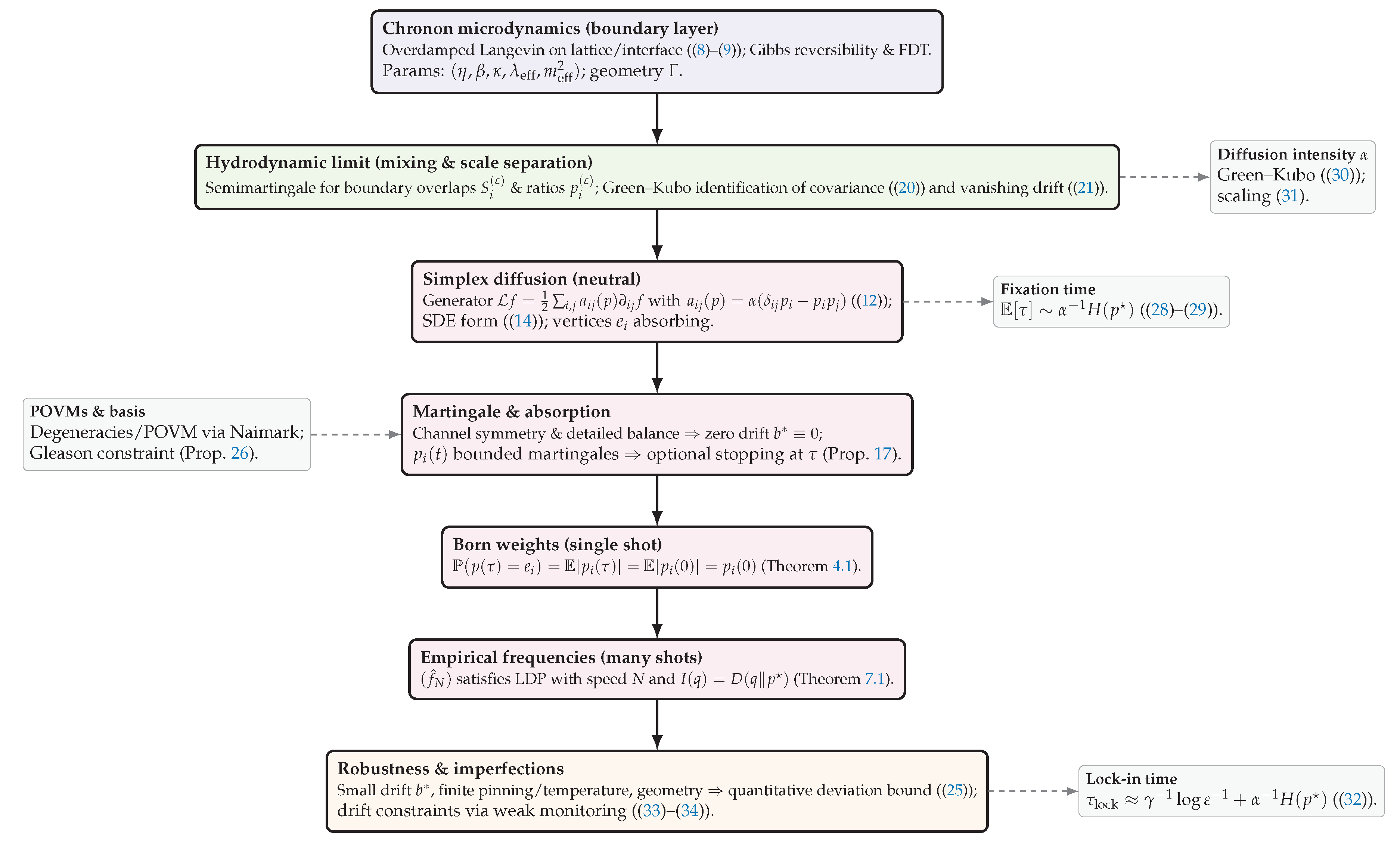
Figure 2.
(a) The apparatus defines stabilized eigen–domains on the interface . A microscopic chronon field, prepared in a superposition , couples locally to and stochastically aligns with one domain. (b) The overlap process diffuses as a bounded martingale and is absorbed at a vertex ; the hitting probabilities equal the initial overlaps (Born rule).
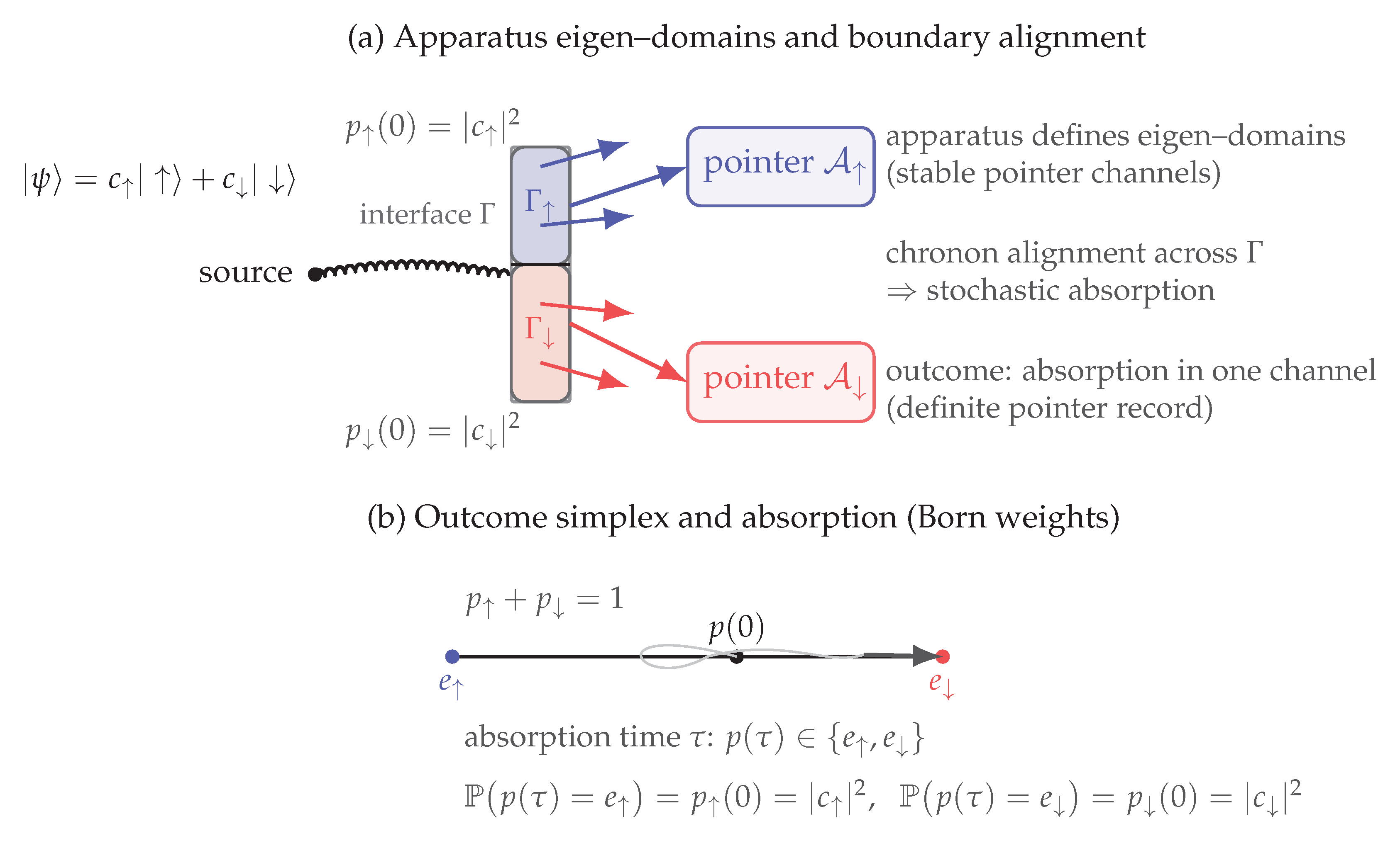
Disclaimer/Publisher’s Note: The statements, opinions and data contained in all publications are solely those of the individual author(s) and contributor(s) and not of MDPI and/or the editor(s). MDPI and/or the editor(s) disclaim responsibility for any injury to people or property resulting from any ideas, methods, instructions or products referred to in the content. |
© 2025 by the authors. Licensee MDPI, Basel, Switzerland. This article is an open access article distributed under the terms and conditions of the Creative Commons Attribution (CC BY) license (http://creativecommons.org/licenses/by/4.0/).
Copyright: This open access article is published under a Creative Commons CC BY 4.0 license, which permit the free download, distribution, and reuse, provided that the author and preprint are cited in any reuse.


