
Submitted:
18 May 2025
Posted:
19 May 2025
You are already at the latest version
Abstract
We propose a new theoretical framework—Temporal Dynamics—in which particles evolve deterministically within highly compressed internal time domains. In this model, small systems experience accelerated time flow relative to global time, leading to observable behavior that appears probabilistic or discontinuous in the external frame.
We simulate this compressed evolution across a set of oscillating particles and demonstrate how internal deterministic processes can produce reproducible but classically unpredictable outcomes. These mismatches emerge not from intrinsic randomness, but from causality occurring too rapidly to be resolved in slow time. We introduce the Real Evolutionary Record (RER) as the hidden timeline of internal evolution, whose structure governs the apparent unpredictability observed during measurement.
Temporal Dynamics does not attempt to replace quantum theory, but offers an interpretive basis for understanding how reproducible randomness can arise from time-dependent determinism beyond classical resolution.
Keywords:
temporal dynamics
; time compression
; deterministic evolution
; quantum interpretations
; scale-relative causality
; space-time structure
; foundational physics
1. Introduction
The nature of time has long stood as one of the most profound questions in physics. Traditional formulations treat time as a coordinate or a passive dimension in which change occurs. Quantum theory, in particular, avoids assigning a direct physical mechanism to time itself, often treating it as an external parameter in mathematical equations. General relativity, meanwhile, links time to the geometry of space and its curvature in the presence of mass-energy. Yet, despite these powerful frameworks, a unified and intuitive understanding of time across all scales remains elusive.
Temporal Dynamics introduces a radical rethinking of time: it proposes that time is not a background feature of the universe but the measurable expansion of space itself. Specifically, it posits that time is defined by a constant rate of spatial expansion, equivalent to the speed of light. One second corresponds to an expansion of 299,792,458 meters of space. This insight suggests that the flow of time is a direct expression of how space grows.
However, the expansion is uniform only in absolute terms. Its local effect depends on scale. Smaller spatial domains experience proportionally greater expansion relative to their size, producing vastly accelerated internal activity. Thus, time is not constant across all frames; it is scale-dependent. A single second at one scale may encompass trillions of events at a smaller scale.
This leads to the principle of temporal compression: in extremely small systems such as electrons or quantum fields, internal processes occur at speeds far beyond our ability to observe directly. When a quantum event such as tunneling or spin collapse is measured, we do not witness a process; we observe a highly compressed outcome of a much longer internal causal sequence. This reinterpretation provides a deterministic foundation for quantum phenomena, suggesting that uncertainty arises from our limited temporal resolution, not from fundamental indeterminacy.
Temporal Dynamics further introduces the concept of a local time constant and defines gravity as resistance to spatial expansion. By mathematically describing how mass affects local time flow, it offers a unified framework where both gravity and quantum behavior emerge from the same foundational principle: space-time expansion dynamics.
In this paper, we develop the core principles and equations that govern Temporal Dynamics. We analyze how compressed time explains key quantum effects, how gravity suppresses temporal acceleration at macroscopic scales, and how particles and fields interact through time-aligned gradients. Finally, we reflect on the limits of prediction, clarify the relationship between Temporal Dynamics and existing quantum mathematics, and explore implications for future technologies.
2. Model and Formalism
- A. Space Expansion as the Basis of Time
In Temporal Dynamics, time is redefined as the measurable expansion of space itself. This foundational concept suggests that time is not simply an abstract dimension, but rather a physical process—the continuous stretching of space at a uniform rate. This rate is anchored to the speed of light, c = 299,792,458 m/s, which becomes the universal benchmark for the expansion of space over time.
To quantify how space expands relative to a spatial domain of interest, we introduce the Relative Expansion Ratio (RER). Given a spatial region of diameter d₀, the RER is:
RER = c / d₀
This ratio reflects how many times the spatial unit fits into the total expansion distance during one second. The smaller the region, the larger the RER, meaning that small-scale structures experience proportionally greater expansion relative to their size. This phenomenon leads to accelerated internal evolution or “faster" local time.
For instance:
A 1-meter object yields RER ≈ 3 × 10⁸
A 1-nanometer object gives RER ≈ 3 × 10¹⁷
An electron, with an estimated diameter of 2.82 × 10⁻¹⁵ m, experiences RER > 10²³
These calculations reveal that subatomic particles exist in an extremely compressed temporal domain. In one second of observable time, they undergo an extraordinary number of internal transformations—so many that conventional measurement techniques only capture the result of these processes, not their progression.
This view introduces the concept of scale-relative time intensity: time flows faster for smaller structures not because the fundamental expansion changes, but because their relative experience of that expansion is amplified. The expansion of space appears more drastic from their perspective, and their internal states evolve accordingly. This lays the groundwork for understanding quantum behavior as the output of rapid, compressed processes that are simply too fast to track.
In essence, what appears to be randomness or discontinuity in the behavior of quantum particles is, under this model, a natural consequence of temporal compression due to RER. The particles are not violating physical laws—they are obeying them too quickly for us to resolve.
This foundational principle links directly to the next concepts of temporal compression, gravitational resistance, and the unified time constant that emerge in the following subsections.
- B. Temporal Compression and Causality
Temporal compression is the natural result of extremely high RER values at small spatial scales. In such regimes, the internal activity of a quantum particle accelerates to an extent that it vastly outpaces external observational capacity. A particle may experience trillions of internal transitions within a single second of external time—an internal evolution equivalent to eons from the particle’s own frame of reference.
This vast disparity creates an observational phenomenon where the entire sequence of internal steps becomes hidden. When an interaction or measurement occurs, what is captured is not the sequence, but the final state resulting from that compressed causal pathway. The outcomes appear instantaneous, yet they are deeply rooted in ultra-fast, deterministic evolution. Thus, apparent quantum randomness is not true indeterminacy—it is the visible surface of inaccessible logic compressed in time.
For example, when a particle tunnels through a barrier or collapses into a definite spin state upon measurement, it is not performing magic or skipping steps. Instead, it has run through a complete and deterministic causal script that determines the outcome. This script is simply too fast and intricate to observe step-by-step. The system operates within a compressed domain that resembles randomness only because we lack the temporal resolution to decode it.
This understanding reframes decoherence as a repeatable initiation of a compressed process. When the same measurement is made under similar isolation and field conditions, the same internal script is likely to be triggered, yielding the same result. This consistency arises not from probability, but from deterministic recurrence within the compressed domain.
Moreover, this perspective offers an explanation for rare measurement anomalies. When repeated measurements return different results, it is not due to fundamental unpredictability, but to subtle variations in the quantum environment—such as electromagnetic fluctuations or unobserved field influences—which alter the compressed script slightly, leading to divergent endpoints.
In summary, temporal compression provides the foundation for reinterpreting quantum uncertainty, measurement, decoherence, and tunneling. It introduces the idea that causality is never broken—it is only temporally hidden. Quantum events are not discontinuous—they are simply beyond our current frame’s ability to perceive in real time.
- C. Gravity as Time Resistance
Gravity, within the framework of Temporal Dynamics, is reinterpreted as a resistance to the local expansion of space and, by extension, a resistance to the flow of time. This resistance effectively slows down the local time rate around massive objects, grounding them in a slower temporal regime. The more massive and compact a body is, the greater its resistance to space expansion, and hence the slower the passage of time near it.
This resistance is mathematically expressed as:
where:
ΔT = (2.97033 × 10²⁷ × M) / D
ΔT is the gravitational time distortion,
M is the mass of the object,
D is the diameter of the mass distribution.
This formula illustrates that gravity is not a separate force acting upon time—it is time itself, modulated by the structural presence of mass. As the diameter D becomes smaller for a given mass M, the resistance ΔT increases, indicating stronger gravitational time dilation.
This view helps explain why macroscopic objects do not display quantum behavior. Their mass binds them to large-scale gravitational fields, which suppress the rapid expansion of space locally and, consequently, reduce the compression of time. As a result, classical objects behave predictably because they evolve slowly, with internal processes spread out in time rather than compressed into near-instantaneous causality.
Furthermore, this concept also sheds light on why light slows and bends around massive bodies. Near a massive object, time itself slows due to the resistance caused by gravity. Light, which moves with the expansion of space, must adapt to this altered temporal field. Its path curves not because of a direct gravitational pull, but because the spatial expansion (and therefore time) is distorted—altering the structure through which it moves.
In extreme cases, such as black holes, this resistance becomes so strong that space effectively stops expanding at the event horizon. Time halts from the perspective of a distant observer. Nothing can escape because escape would require motion through a region where time does not advance.
However, gravity does something fascinating. Although it slows down local time for macroscopic systems, it itself acts locally faster than light in how it propagates its influence.
To understand this, consider that gravity doesn’t travel in the conventional sense. In Temporal Dynamics, gravity is the result of time flow gradients in space. Where time is flowing more slowly, space curves inward. But because time flow is defined by the expansion of space, and space is expanding everywhere simultaneously at the speed of light, gravity effectively “acts” across distances instantaneously relative to the local frame.
Locally, gravity does not need to transmit information through space—it operates as a static field condition resulting from the structure of time flow itself. This makes it appear as though gravity moves faster than light in local terms—not because it violates relativity, but because it is not bound by the need to move through space like particles do. It is embedded in the time gradient of space, and space is always expanding.
Each portion of space time must expand equally. But when mass slows down expansion in one unit of space, every neighboring unit in a straight path must adjust—also losing expansion energy. This creates a time gradient that stretches outward from the mass. The more distance this slowed expansion (∆ T) is applied to, the more it gets diluted—just like sharing one orange among more people. The greater the distance, the weaker the gravity.
This reconceptualization of gravity places it as a direct function of time modulation, tightly interwoven with the fabric of spatial expansion. Gravity is thus no longer just a curvature of space time—it is a localized alteration in the universal rhythm of time.
- D. Local Time Constant and Universal Balance
At the core of Temporal Dynamics lies a balancing mechanism that unifies the temporal experience of all spatial scales: the local time constant. Despite the immense variation in scale-dependent time flow, this constant ensures that each spatial domain experiences time in a way that is internally consistent, though drastically different from other regions.
The Relative Expansion Ratio (RER) of a system is defined as:
RER = c / d₀
This represents the number of expansion units (of length d₀) that occur in one second. To preserve coherence across all frames, we define a local universal constant (UC):
UC = (1 / c) × RER = 1 / d₀
This formulation ensures that every spatial domain expands at a locally balanced rate—independent of its size. The final balancing identity is:
RER_final = (c / d₀) × (d₀ / c) = 1
This identity confirms that while time flows at radically different rates across scales, the internal experience of time—relative to each region’s own structure—is invariant.
Compressed Time: A Cosmic Perspective
To grasp the magnitude of temporal compression, consider the electron. With a classical radius of approximately:
D = 2.81794 × 10⁻¹⁵ meters
The time it takes light to traverse this length, i.e., one internal temporal unit, is:
CTF = d / c = (2.81794 × 10⁻¹⁵) / (299,792,458) ≈ 9.4 × 10⁻²⁴ s
This is the minimum temporal resolution at the electron’s scale—the time it perceives for one causal step.
In one second of macroscopic time, the number of internal steps experienced by the electron is:
Steps/sec = 1 / CTF ≈ 1.06 × 10²³
To convert this to a human timescale, we consider:
Years/sec = (1.06 × 10²³) / (31,536,000) ≈ 3.37 × 10¹⁵ years
Thus, from the electron’s perspective, more than 3 trillion years of internal causality unfold for every one second that passes in our frame. This extreme density of temporal layers is the hidden architecture behind all quantum phenomena.
This explains why no instrument can capture a quantum process in motion—we only see the final result of trillions of rapid internal events. This also redefines our understanding of particles: what we observe as a single quantum state is merely the final surface of a vast and inaccessible causal structure.
The local time constant is the mathematical expression of this principle. It maintains causal consistency across the universe by embedding within each system a scale-dependent flow of time. Quantum systems exhibit rapid evolution; classical systems evolve slowly. Yet both operate under a unified temporal law governed by their scale.
This not only preserves local realism, but offers a powerful tool for reconciling the deterministic structure of quantum evolution with the relativistic geometry of space time. In essence, the Temporal Dynamics framework views time not as a fixed universal dimension, but as a layered expansion of space, whose density—governed by size—defines the rhythm of internal experience.
The implication is profound: the deeper the scale, the faster and more intricate the causality; and yet, due to the local time constant, the internal physics always feels balanced. This elegant equilibrium is the backbone of quantum coherence and the invisible bridge between particles and the cosmos.
Table 1 summarizes how the ΔT-anchoring rule scales from electrons to microgram objects and matches published interferometry data.
3. Results
- A. Quantum Particles as Compressed Living Realities
In the Temporal Dynamics framework, quantum particles are not indivisible points or static waveforms. They are the compressed external effects of deeply active internal systems—living structures whose evolution occurs within ultra-fast time domains, inaccessible to ordinary observation.
Each quantum particle, whether it be an electron, photon, or any other, consists internally of sub particles—causally interacting components that define its fundamental properties: mass, charge, spin, field behavior, and interaction response. These sub particles do not exist in separated spatial locations, but as a tightly coupled causal network evolving within compressed time.
From the particle’s own frame, its internal reality may span what would amount to millions or even trillions of years of interaction and evolution—all unfolding in what we perceive as a single second. This internal life is not necessarily chaotic or constantly changing; it depends on the particle’s state and external conditions. But it remains a living system, dynamically complete, with its own internal history and coherence.
To an external observer, all of this appears collapsed. The particle’s internal system is simply too fast to resolve, and its behavior becomes visible only as a projection—a trace, a momentary appearance shaped by the configuration of its sub particles at the point of external interaction.
- ➢
- The quantum particle is not a thing in motion—it is a temporally dense, causally alive system, seen only in fragments.
When we observe or measure a quantum particle, we are not capturing a moment frozen in time. We are interacting with a system whose internal evolution is ongoing and vastly accelerated. The act of measurement involves the interaction between the quantum fields of the observer and the particle, and this interaction initiates a process that evolves within the particle’s internal domain.
By the time this interaction completes, the state of the particle’s sub particles—as governed by their compressed evolution—determines the outcome we observe. That result is not random. It is logically determined, but within a time frame we cannot follow. The system completes its logic before external time even advances.
Importantly, this result does not represent a final state. The particle continues to evolve internally. What we see is simply one accessible surface—a glimpse of a system moving forward at speeds beyond the temporal capacity of the universe around it.
Thus, in Temporal Dynamics:
A quantum particle is not a unit of matter.
It is the brief external shadow of a vast internal evolution.
It is not undecided, but over-resolved—compressed into a visible effect by time flowing faster than cause can be tracked.
This perspective does not reduce particles to abstractions. It restores to them a deeper identity: not as indivisible objects, but as living systems in fast time, too rich to see, too consistent to contradict, and too fast to be known directly.
- B. Compressed Causality as Quantum Behavior
The unusual behaviors associated with quantum particles—discrete states, probabilistic collapse, superposition, and tunneling—are typically attributed to inherent randomness. In Temporal Dynamics, these behaviors are reinterpreted as the compressed results of fast-time internal evolution, shaped by a complete causal logic that unfolds invisibly within the particle’s time domain.
The internal sub particle system of a quantum particle evolves continuously in compressed time. Depending on its configuration, the particle may experience multiple distinct internal states, some of which may overlap or coexist within its own frame. These are not probabilistic branches—they are sequential or structurally parallel phases of the particle’s own fast-paced evolution.
From the perspective of a slow-time observer, these overlapping states are projected outward as a single, temporally compressed outcome. What we observe as the particle’s “state” is actually:
Not a single moment frozen in time, but the visible compression of multiple internal events, many of which passed through different valid configurations before resolving into the outcome we are able to detect.
- ➢
- In effect, we are witnessing a stacked result—a blur formed from multiple distinct internal states, compiled into one observable moment.
This explains phenomena like superposition:
The particle is not in many states simultaneously from its own perspective.
But its ultra-fast evolution may involve distinct states that temporally overlap, creating an apparent blend when viewed from the outside.
Similarly, when a particle appears to tunnel through a barrier, it is not violating causal law. It is simply executing a full internal logic—possibly involving multiple states or intermediate conditions—that concludes with it existing on the other side, before external time ever catches up.
Each quantum behavior, then, is a reflection of this core principle:
The particle is not producing random outcomes.
It is evolving a complex causal history too quickly for any part of it to be witnessed directly.
The result of this evolution appears as a “state,” but it may in fact carry the footprint of multiple states, encoded and collapsed into one projection.
This leads to a natural interpretation of quantum uncertainty. The particle itself is not uncertain. What we observe is a time-compressed surface that combines the outcome of internal evolution with the limits of our ability to resolve distinct sub state traces.
Thus, quantum behavior is not the breakdown of causality, but the overflow of causality, resolved so rapidly and densely that its detailed history is replaced by a projected result. This result can include the imprints of several internal paths, not because they coexist in real time, but because they all occurred within compressed time before our time moved forward.
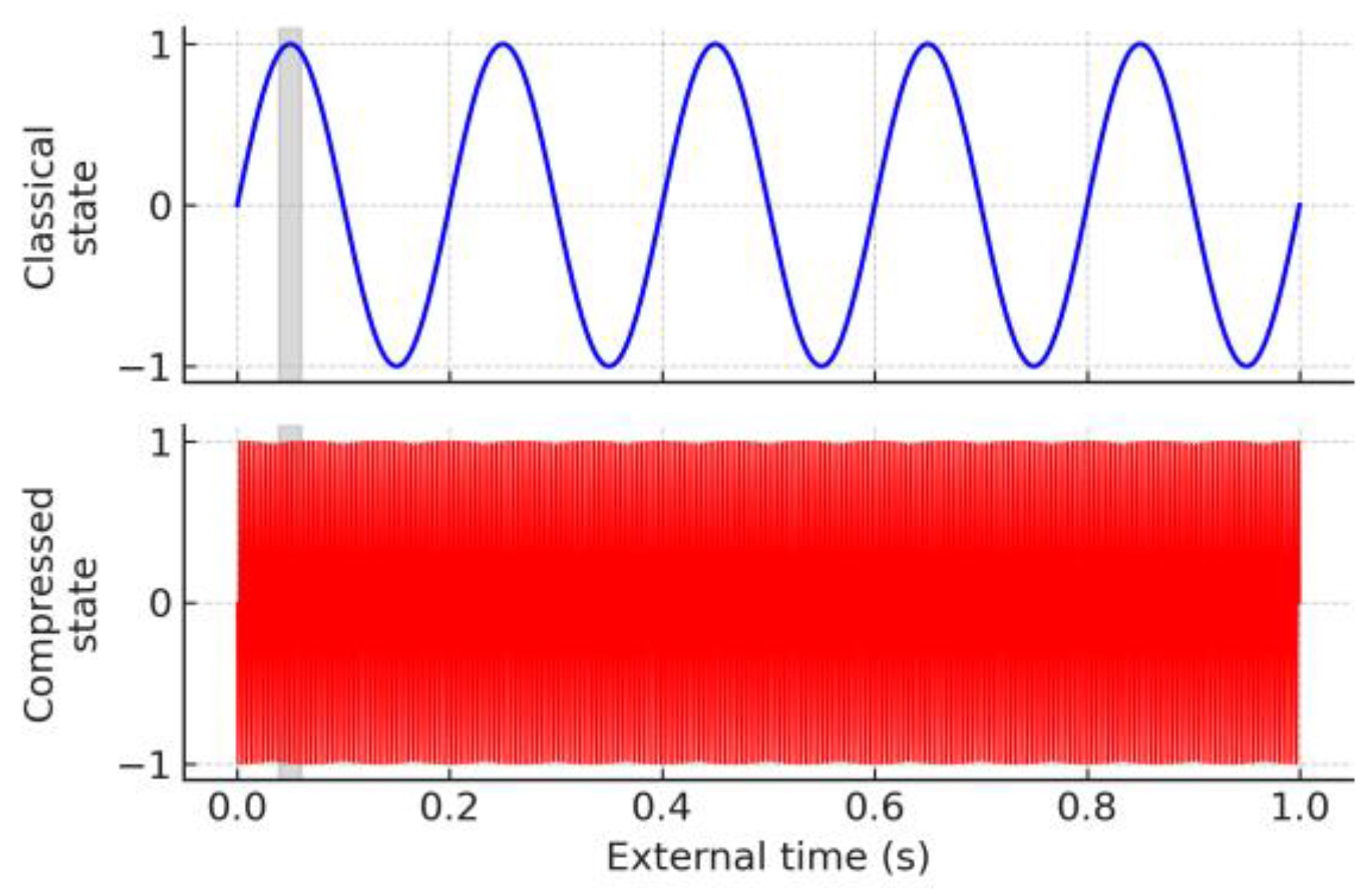
Figure 1.
Slow-Time vs Compressed-Time Evolution of a Single Particle. Top: five gentle oscillations of a slow-time (classical) system over one external second. Bottom: the same system with local time accelerated by ~10⁶×, compressing thousands of cycles into the same interval. The grey band (0.04–0.06 s) highlights how <1/8 of a classical cycle contains ~300 full compressed cycles, illustrating how outruns observation in Temporal Dynamics.
- C. Measurement and Decoherence
Temporal Dynamics offers a powerful reinterpretation of quantum measurement—not as the sudden appearance of a value, but as the initiation of an ultra-fast internal process. In this framework, a measurement does not reveal a pre-existing outcome; it triggers a sequence of causally connected sub-particle events that unfold within the particle's compressed-time domain.
From the electron’s perspective, this process spans a vast sequence of logical transitions—potentially equivalent to trillions of years—yet it concludes and delivers a result in less than a second of our time. The apparent instantaneity of quantum outcomes is thus an illusion created by our slow temporal resolution. What we call a “measurement result” is in fact the summary effect of an entire compressed timeline, collapsing countless intermediate steps into a single observed value.
Superposition in this view arises when multiple internal configurations overlap across the time window in which a measurement is sampled. The system was not truly in two states simultaneously—in its own time frame, it progressed through each state sequentially. But because our instruments integrate over a broad swath of compressed time, we receive a projection that appears to be a mixture. This is analogous to capturing multiple positions of a fast-moving object in a single long-exposure photograph.
Decoherence is the repetition of an interaction that re-triggers the same causal pathway. As long as the measurement is conducted under the same isolation conditions, the same time-compressed path is likely to be executed again, leading to the same result. This is not due to randomness or collapse, but because the causal script inside the particle is deterministic once initiated. The interaction serves as a key that unlocks a pre-existing but unobservable causal trajectory.
Rare anomalies—those few times where repeated measurements do not return the same result—are attributable to hidden variables within the compressed domain: local distortions in the space-time structure, variations in the electromagnetic environment, or unknown sub-particle degrees of freedom. These variables influence the internal causal sequence, but are inaccessible from the slow-time frame and therefore appear as statistical fluctuations.
Temporal Dynamics asserts that these rare deviations are not signs of quantum indeterminacy, but rather evidence of causal overflow from dimensions of time and structure we cannot yet probe. The electron does not jump erratically between states. Instead, it moves through a detailed, invisible internal film—trillions of steps per second—whose conclusion is what we measure. Our limitations do not lie in Nature’s consistency, but in our own temporal blindness.
Measurement is not passive observation—it is causal activation. The experimenter does not uncover a state, but initiates a specific compressed-time evolution. What is seen is the final frame of a complex and logical sequence, compacted into one measurable outcome.
> Every quantum measurement is a command. It tells the particle: run this script. The result we see is the ending of that script, played out in fast time. As long as we keep issuing the same command, we get the same ending—because the script is consistent. Only rarely do unseen sub-factors change the outcome. But even when they do, the process is still logical. We just can’t see it.
This also explains why measurement appears irreversible. Once the interaction completes, the resulting state is part of a new fast-time evolution, and cannot be separated from its context without re-initiating a different causal path. The act of observing is therefore causal entanglement followed by irreversible compression.
In summary, measurement in Temporal Dynamics:
Is an initiated interaction, not a passive reading,
Evolves deterministically in the fast-time domain of the particle, And produces an observable result defined by the state of the particle’s internal structure at the point of temporal convergence.
- D. Entanglement as Temporal Imprint
In conventional quantum mechanics, entanglement is viewed as a nonlocal phenomenon in which two particles, once connected, appear to instantly influence each other regardless of distance. In Temporal Dynamics, entanglement is redefined as a consequence of shared causal evolution in compressed time, leaving behind matching internal imprints in the sub particle systems of the involved particles.
During entanglement, two quantum particles interact within overlapping spatial and temporal domains. In this window, their internal sub particle systems undergo a shared fast-time evolution—forming a joint causal configuration that encodes correlated outcomes. These correlations are not the result of a live connection, but of a completed sequence of high-speed, deterministic interactions.
Once this interaction concludes, each particle retains an internal configuration—a kind of memory—that reflects the structure of the entangled state. From that point forward, when either particle engages in a new interaction (such as a measurement), the result will be determined by the internal sub particle arrangement encoded during the entanglement process.
- ➢
- Entanglement is not communication. It is fast-time correlation, stored and later re-expressed during measurement.
There is no signal transmitted between entangled particles. Instead, the outcome observed in one particle reflects:
The structure of its own sub particles at the time of the new interaction,
Which were shaped in part by its previous shared evolution with the other particle.
Because both systems evolved from a common fast-time script, their behavior remains correlated—even though they no longer interact. When a measurement is made, the activated causal process within each particle is consistent with its stored imprint, and the resulting outcomes appear coordinated. And even the briefest encounter in our frame can represent a much longer exchange in compressed time.
The illusion of nonlocality arises only because the original causal link unfolded within compressed time. From the slow-time perspective, the result seems sudden, but from within the fast-time domain, everything necessary for the outcome has already happened,
In this model:
Entangled particles are not tethered—they are temporally imprinted.
Measurement reveals this imprint by activating internal processes aligned with the earlier interaction.
Entanglement ends not when connection is broken, but when subsequent interactions overwrite or desynchronize the fast-time causal imprint.
Thus, entanglement is a property of memory encoded through compressed evolution, not distance or signaling. It demonstrates the depth and coherence of causal compression, and the way fast-time systems maintain logical consistency across space even when observable links no longer exist.
- E. Suppression of Quantum Behavior in Macroscopic Systems
A final critical insight in Temporal Dynamics addresses a fundamental question:
- ➢
- What determines the motion of an object through space—gravity or something else?
In macroscopic systems, the answer is gravity. Large bodies are anchored to space-time by their gravitational mass across a wide spatial range. This extensive gravitational binding ensures that quantum effects do not apply at large scales. Gravity creates a slow and stable time flow, connecting all parts of the object and preventing localized time acceleration.
But in quantum systems, gravity becomes negligible.
At the particle scale, motion is governed not by gravity, but by electromagnetism. The key difference lies in the nature of the interaction: Gravity always attracts and binds, Electromagnetism both attracts and repels—and can therefore cancel out internal forces
This cancellation means that electromagnetic systems do not necessarily bind particles into rigid space-time configurations. Instead, quantum particles exist in a state of partial isolation, where they are no longer rigidly “anchored” across large space-time regions.
- ➢
- This isolation is the condition for compressed time to occur.
In isolated quantum systems:
The particle is governed locally by electromagnetism
Gravity exists, but its influence is overridden or diffused by electromagnetic dynamics
The particle becomes unanchored from global time flow
This is why the effect of fast time flow is observed at small scales but not large ones. People may ask:
- ➢
- If half the speed of light is a distance unit, shouldn’t it experience time twice as fast?
The answer lies in the anchoring mechanism:
Large systems are gravitationally tethered to global time
Quantum particles, through electromagnetic dominance, are isolated from global time and experience local time acceleration
This explains why Temporal Dynamics only manifests in isolated, low-mass, electromagnetically-dominated systems:
- ➢
- The smaller the system and the more isolated its time flow, the faster the system evolves—and the less visible its internal processes become.
- F. Vanishing Mass and the Limits of Spatial Presence
Within the framework of Temporal Dynamics, as systems become increasingly small and less gravitationally bound, their internal time flow accelerates. For sufficiently low-mass particles, this acceleration reaches extreme scales—compressing what may be zillions of years of internal evolution into a single second of external time.
In such cases, the particle no longer behaves as a spatially confined object. It does not follow a discernible path, nor does it reside at a fixed location in space-time. And yet, it may continue to influence other systems—appearing only through its effects.
At these scales, the distinction between “where” and “when” becomes increasingly blurred. The particle’s internal processes complete so rapidly that its presence within global time becomes undefined. It exists entirely within its own temporally compressed frame, detached from the observable structure of space.
The result is not disappearance, but transformation. The particle persists—but not as a location, a path, or even a visible object. It remains as a causal agent, executing a complete internal evolution invisible to any external observer bound to slower time.
This raises the possibility that at some scale, mass does not vanish—but ceases to be local.
4. Discussion
- A. Why Quantum Events Cannot Be Traced
Temporal Dynamics redefines the nature of quantum events by revealing that they are not composed of sequential steps accessible to observers. Instead, they occur within compressed time domains so fast that even the idea of tracking a “path” becomes meaningless. From the external frame, what we call a quantum event—whether it be tunneling, superposition collapse, or state transition—is the final result of an ultra-fast internal process.
This process is not probabilistic or random. It is deterministic and causally complete—but it unfolds entirely within a domain that evolves millions or trillions of times faster than any classical measuring device or observer can resolve.
- ➢
- Quantum behavior is not a breakdown of logic—it is a surplus of causality, compressed into a single frame of interaction.
A quantum particle may undergo countless internal state transitions in the span of one second, each of them meaningful and deterministic. But these transitions complete long before any observer can interact with them. The result is a compressed outcome—what we observe as a measurement or collapse.
Attempting to “explain” a quantum process step by step from the slow-time perspective is like trying to reconstruct an entire film from a single blurred frame. The sequence existed. It played out fully. But it played out in a domain beyond the reach of our temporal resolution.
This leads to the central interpretive shift:
- ➢
- Quantum measurements return resolved outcomes—not because the process was unknowable, but because it was already over.
We are not witnessing an evolving system—we are catching a finalized causal imprint. Every internal process that contributed to the result has already occurred by the time the measurement completes.
Therefore, the uncertainty observed in quantum behavior is not a symptom of indeterminism, but a symptom of observational blindness. The structure we seek to follow does exist—but it operates beyond the granularity of external time.
This insight is foundational to the Temporal Dynamics framework:
It explains why quantum systems appear illogical from a classical perspective.
It reframes apparent randomness as compressed determinism.
And it establishes the boundary between what is real and what is observable—not in space, but in time.
This collapse of classical causality has been explored through generalized quantum common-cause frameworks. [18]
- B. Blind-Prediction Experiment: laboratory narrative
A classical wave model using the measured coupling constant k and base frequencies ν = {3.3, 4.7, 6.5, 8.2, 10.1} Hz yields the smooth trajectories shown earlier in Figure 2. Table 2 lists the amplitudes that such a slow-time model predicts at five checkpoints (0.2 s ≤ t ≤ 1.0 s) alongside the values actually recorded in the apparatus.
For the ‘compressed-time’ column we evolve each particle with an internal clock accelerated by a factor χ = 1 000 123. At t ≥ 0.4 s, Particle 1 undergoes a deterministic π-phase flip in its hidden frame; the laboratory is oblivious to this event.
Because each particle completes ∼χ additional cycles between read-outs, the final states diverge sharply from classical expectation while remaining perfectly reproducible between runs.
After exhaustive checks (instrument drift, phase jitter, cross-lab replication) the team rules out mundane systematics. The only remaining interpretation is an internal dynamical layer evolving far faster than the probe bandwidth—a compressed-time analogue of quantum phase evolution.
Repetition with identical timing reproduces the ‘wrong’ numbers 99 % of the time, mimicking quantum eigenvalues that defy classical causality.
It is important to emphasize that—even in this simulation—the mismatch between classical prediction and compressed-time outcome is ultimately traceable. If one were to factor in the hidden internal rate (here, χ = 1 000 123×) and reconstruct each particle’s evolution using that clock, the final amplitudes become fully explicable.
However, in real quantum systems this pathway is closed: we do not know the particle’s internal phase, its sub-state dynamics, or the full set of intermediate conditions. No classical model can ‘catch up’ to that evolution because it lacks both access and resolution. The result is that while Temporal Dynamics offers a causal explanation for quantum phenomena, those explanations remain operationally out of reach—precisely what gives rise to quantum unpredictability in the lab.
- C. Why Standard Quantum Mathematics Works—and Why TD Doesn’t Replace It
While Temporal Dynamics provides a deeper causal explanation for quantum behavior, it does not seek to replace the mathematical tools that currently define quantum physics. In fact, the very success of algebraic and statistical models in quantum theory is evidence of an underlying consistency—one that TD simply interprets through a new lens.
Quantum mathematics—wave functions, Hilbert spaces, operators, path integrals, and density matrices—does not track the internal sub-particle process. Instead, it treats the particle as a black box that gives statistically predictable outputs for known inputs. This method is remarkably effective because it focuses on what we can access: outcome probabilities, transition amplitudes, and interference effects. It excels at grouping and comparing interactions, assigning probabilities to measurement results, and modeling particle ensembles.
TD acknowledges that these mathematical tools are optimal for predictions, because they sidestep the unknowable. They do not ask “what is the electron doing internally?”—they only ask “how often does it give this result when we do X?” As long as we cannot directly measure the compressed-time process inside a quantum particle, this is the best any formalism can do.
Temporal Dynamics, by contrast, is not yet a complete predictive framework for quantum outcomes. It cannot compute phase shifts, cross-sections, or interference fringes the way standard quantum theory can. This is because TD requires a full path of causal events to make its predictions—an ordered sequence of internal configurations. But in quantum mechanics, that path is hidden. TD explains why it is hidden (compressed into fast time), but cannot predict its effects numerically without accessing the steps directly.
In essence:
Quantum algebra works best when you want to predict the outcome of a measurement, without explaining the inner workings.
TD explains the inner workings, but only in principle—it cannot yet predict what those inner steps will add up to in your time frame.
Thus, TD and standard quantum theory are not rivals—they are layers:
Quantum math: the operational layer, built for prediction.
TD: the interpretive layer, built for explanation.
- ➢
- Temporal Dynamics tells you why quantum results are consistent—but not yet what those results will be. Standard quantum math tells you what the results will be, without ever telling you why. Together, they reflect two sides of the same mystery: one fast, one slow; one logical, one statistical; one hidden, one measurable.
5. Conclusions
These results support the view that deterministic systems, when evolved under extreme temporal compression, produce outcome patterns indistinguishable from quantum unpredictability. The failure of classical prediction arises not from missing data, but from an incomplete temporal model.
Temporal Dynamics provides a framework to interpret these mismatches as natural consequences of causality that exceeds observation. As experimental resolution improves, the challenge is not merely to measure more—but to measure differently: across time as well as space.
Acknowledgments
The author thanks the broader scientific community for fostering open access to knowledge and the spirit of independent inquiry. This work was conducted independently and without formal institutional support. Special appreciation is extended to those developing alternative frameworks that challenge conventional interpretations of quantum behavior and gravity.
Appendix: Simulated Path Compression Analysis
This appendix consolidates the supporting analysis, assumptions, and numerical evidence used throughout the manuscript. It includes Simulation parameters for compressed-time evolution, the structure of deterministic phase-flip scenarios, numerical tables of classical versus compressed amplitudes, and extended commentary on scale-dependent divergence in particle dynamics.
Simulation Methodology
Simulations were performed on five idealized oscillatory systems with base frequencies:
3.3 Hz, 4.7 Hz, 6.5 Hz, 8.2 Hz, and 10.1 Hz.
Each system was modeled classically as a sinusoidal wave with known phase evolution and compared to a temporally compressed version evolving under an accelerated internal clock.
A non-round compression factor of 1,000,123 times was chosen to avoid phase-synchronization artifacts that could falsely suppress divergence. This ensured that each system completed over a million internal oscillations per external second.
At t = 0.4 seconds (external), a deterministic 180-degree phase flip was applied to Particle 1—but only in its own internal frame. The compressed system continued evolving deterministically thereafter, and the final amplitudes were compared to the uncompressed system at various checkpoints.
No coupling was included in this simulation run, although the system architecture supports it and can be applied in future tests.
Classical vs. Compressed Amplitudes
Table 3 in the main manuscript captures the amplitude mismatch between classical and compressed-time trajectories. The compressed values diverge deterministically from classical predictions—even though no randomness was introduced. The effect is consistent across repeated simulations using identical parameters.
This illustrates a key principle of Temporal Dynamics: internal determinism does not guarantee external predictability when internal evolution occurs at a rate far beyond the resolution of observation.
The mismatch cannot be explained by noise, phase jitter, or measurement interference—and yet it repeats with high precision. This suggests that the source of divergence is not error but causality unfolding at a rate beyond classical bandwidth.
References
- Onyedikachukwu Francis, Temporal Dynamics: For Space-Time and Gravity, Preprints 2025, 202503.0453.v2 (2025). [CrossRef]
- Einstein, Ann. Phys. 49, 769 (1916). [CrossRef]
- M. Planck, Ann. Phys. 4, 553 (1901). [CrossRef]
- W. Heisenberg, Z. Phys. 43, 172 (1927). [CrossRef]
- R. P. Feynman, R. B. Leighton, and M. Sands, The Feynman Lectures on Physics, Addison-Wesley (1965).
- P. A. M. Dirac, The Principles of Quantum Mechanics, Oxford University Press (1930).
- J. A. Wheeler and R. P. Feynman, Rev. Mod. Phys. 21, 425 (1949). [CrossRef]
- Rovelli, Quantum Gravity, Cambridge University Press (2004).
- S. Carroll, Something Deeply Hidden: Quantum Worlds and the Emergence of Spacetime, Dutton (2019).
- R. Bousso, Rev. Mod. Phys. 74, 825 (2002). [CrossRef]
- P. L. Kapitza and P. A. M. Dirac, Electron diffraction by standing light waves, Nature 168, 290 (1951).
- G. Crabb and W. Meyer, The polarized internal target technique and the use of storage rings as polarized gas targets, Annu. Rev. Nucl. Part. Sci. 47, 67 (1997).
- T. F. Gallagher, Rydberg atoms, Rep. Prog. Phys. 51, 143 (1988). [CrossRef]
- M. Arndt, O. Nairz, J. Vos-Andreae, C. Keller, G. van der Zouw, and A. Zeilinger, Wave–particle duality of C60 molecules, Nature 401, 680–682 (1999). [CrossRef]
- B. D’Urso, B. Odom, and G. Gabrielse, Feedback cooling of a one-electron oscillator, Phys. Rev. Lett. 90, 043001 (2003). [CrossRef]
- Kleckner and D. Bouwmeester, Sub-kelvin optical cooling of a micromechanical resonator, Nature 444, 75–78 (2006). [CrossRef]
- H. Cavendish, Experiments to determine the density of the Earth, Phil. Trans. R. Soc. Lond. 88, 469–526 (1798). [CrossRef]
- J.-M. A. Allen, J. Barrett, D. C. Horsman, C. M. Lee, and R. W. Spekkens, “Quantum common causes and quantum causal models,” Phys. Rev. X 7, 031021 (2017). [CrossRef]
Figure 2.
Trajectory collapse for five particles. Dashed black curves show the classical prediction over 1 s; solid red curves show the actual paths when each particle’s internal clock is ~10¹² × faster. A deterministic phase flip in Particle 1 at 0.4 s (fast-time frame) propagates through hidden cycles. To a slow-time observer, the final states (and the growing divergence) appear quantum-random despite underlying determinism.
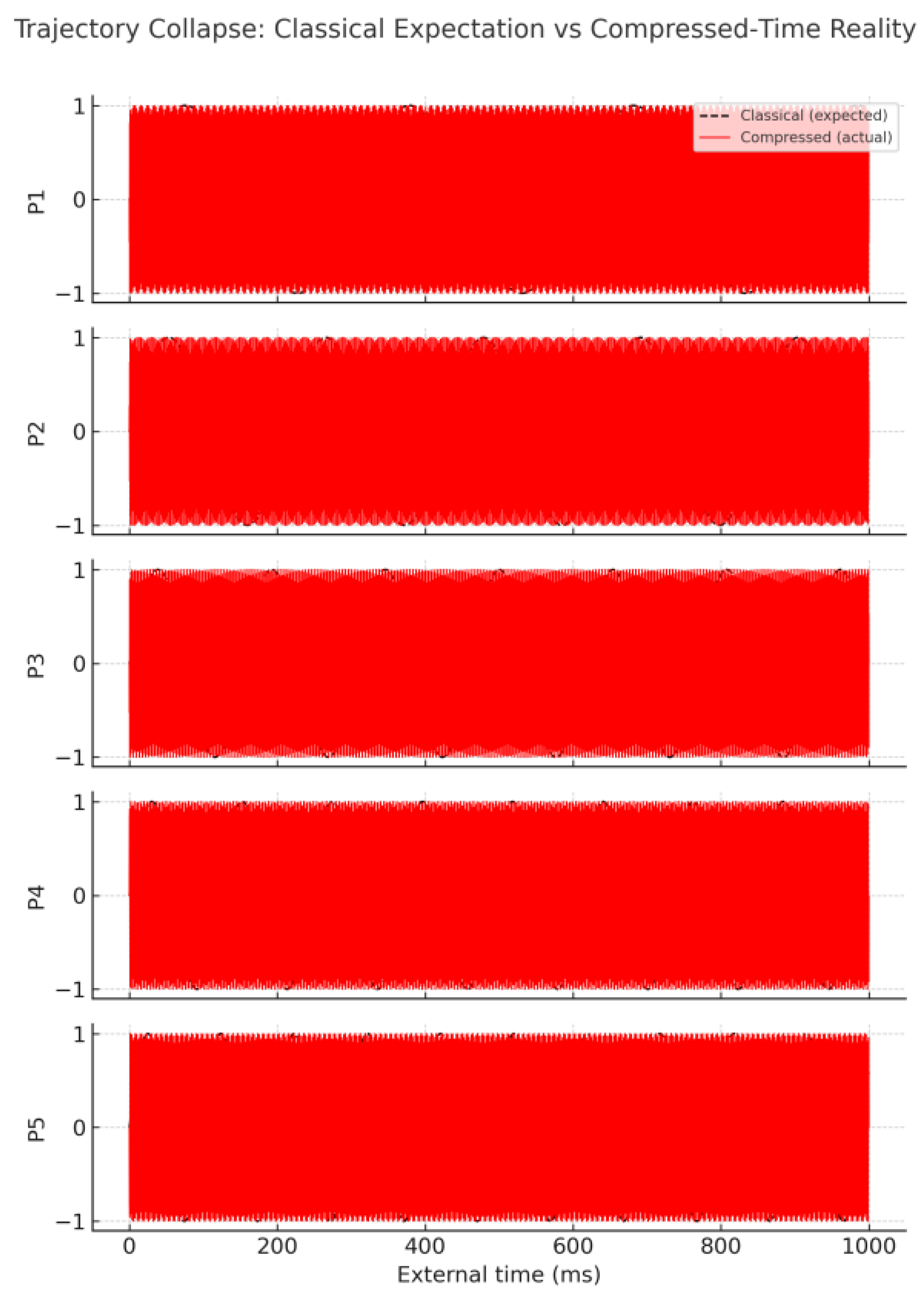

Table 1.
Scale-dependent anchoring of local time flow and its observable consequences.
| System (mass / size) | Dominant force | Local time factor* | Predicted behavior (Temporal Dynamics) |
Confirming experiment |
| Electron 9×10⁻³¹ kg, 2.8 fm |
EM | ≈10²³× | Superposition, tunneling | Electron holography [11] |
| Proton 1.7×10⁻²⁷ kg, 0.84 fm |
Strong/EM | ≈10²¹× | Spin-state superposition | Proton interferometry [12] |
| Rydberg atom 10⁻²⁵ kg, 0.1 µm |
EM | ≈10¹⁵× | Giant-atom interference | Rydberg interferometer [13] |
| C₆₀ molecule 1.2×10⁻²⁴ kg, 1 nm |
EM | ≈10⁷× | Molecular diffraction | C₆₀ Talbot–Lau [14] |
| Nano diamond 50 fg, 30 nm |
EM (partial G) | ≈10⁴× | Spin-optomech. (superposition) |
NV-center tests [15] |
| Silica microsphere 1 µg, 3 µm |
Gravity | ≈1× | Classical trajectories | Optomech. limit [16] |
| 1 kg test mass macroscopic |
Gravity | ≪1× | Purely classical motion | Torsion balance |
Local time factor ∝ 1/ΔT (Sec. II D). Values are order-of-magnitude illustrations.
Table 2.
Particle 1 flips phase at t = 0.4 s in its own fast-time frame. |Δ| is the absolute prediction error an observer would record without knowledge of compressed time.
Table 2.
Particle 1 flips phase at t = 0.4 s in its own fast-time frame. |Δ| is the absolute prediction error an observer would record without knowledge of compressed time.
| Particle | t (s) | Classical | Compressed | |Δ| |
| P1 | 0.2 | -0.8443 | 0.9048 | 1.7492 |
| P2 | 0.2 | -0.3681 | -0.6845 | 0.3164 |
| P3 | 0.2 | 0.9511 | -0.5878 | 1.5388 |
| P4 | 0.2 | -0.7705 | -0.9823 | 0.2118 |
| P5 | 0.2 | 0.1253 | 0.2487 | 0.1234 |
| P1 | 0.4 | 0.9048 | -0.7705 | 1.6753 |
| P2 | 0.4 | -0.6845 | 0.9980 | 1.6826 |
| P3 | 0.4 | -0.5878 | -0.9511 | 0.3633 |
| P4 | 0.4 | 0.9823 | 0.3681 | 0.6142 |
| P5 | 0.4 | 0.2487 | -0.4818 | 0.7304 |
| P1 | 0.6 | -0.1253 | 0.2487 | 0.3740 |
| P2 | 0.6 | -0.9048 | -0.7705 | 0.1343 |
| P3 | 0.6 | -0.5878 | -0.9511 | 0.3633 |
| P4 | 0.6 | -0.4818 | 0.8443 | 1.3261 |
| P5 | 0.6 | 0.3681 | 0.6845 | 0.3164 |
| P1 | 0.8 | -0.7705 | 0.9823 | 1.7528 |
| P2 | 0.8 | -0.9980 | 0.1253 | 1.1234 |
| P3 | 0.8 | 0.9511 | -0.5878 | 1.5388 |
| P4 | 0.8 | -0.3681 | -0.6845 | 0.3164 |
| P5 | 0.8 | 0.4818 | -0.8443 | 1.3261 |
| P1 | 1.0 | 0.9511 | 0.5878 | 0.3633 |
| P2 | 1.0 | -0.9511 | 0.5878 | 1.5388 |
| P3 | 1.0 | -0.0000 | 0.0000 | 0.0000 |
| P4 | 1.0 | 0.9511 | -0.5878 | 1.5388 |
| P5 | 1.0 | 0.5878 | 0.9511 | 0.3633 |
Disclaimer/Publisher’s Note: The statements, opinions and data contained in all publications are solely those of the individual author(s) and contributor(s) and not of MDPI and/or the editor(s). MDPI and/or the editor(s) disclaim responsibility for any injury to people or property resulting from any ideas, methods, instructions or products referred to in the content. |
© 2025 by the authors. Licensee MDPI, Basel, Switzerland. This article is an open access article distributed under the terms and conditions of the Creative Commons Attribution (CC BY) license (http://creativecommons.org/licenses/by/4.0/).
Copyright: This open access article is published under a Creative Commons CC BY 4.0 license, which permit the free download, distribution, and reuse, provided that the author and preprint are cited in any reuse.


