
Submitted:
27 August 2025
Posted:
28 August 2025
You are already at the latest version
Abstract
Background: Electrochemical impedance spectroscopy (EIS) is indispensable for disentangling charge-transfer, capacitive, and diffusive phenomena, yet reproducible parameter estimation and objective model selection remain unsettled. Methods: We derive closed-form impedances and analytical Jacobians for seven equivalent-circuit models (Randles, CPE, Warburg variants), enforce physical bounds, and fit synthetic spectra with 2.5% and 5.0% Gaussian noise using hybrid optimization (Differential Evolution → Levenberg– Marquardt). Uncertainty is quantified via non-parametric bootstrap; parsimony is assessed with RMSE, AIC, and BIC; physical consistency is checked by Kramers–Kronig diagnostics. Results: Rs and Rct are consistently identifiable across noise levels. CPE parameters (Q, n) and diffusion amplitude (σ) exhibit expected collinearity unless the frequency window excites both processes. Randles suffices for ideal interfaces; Randles+CPE lowers AIC when non-ideality and/or higher noise dominate; adding Warburg reproduces the 45◦ tail and improves likelihood when diffusion is present. The (Rct + ZW ) ∥ CPE architecture offers the best trade-off when heterogeneity and diffusion coexist. Conclusions: The framework unifies analytical derivations, hybrid optimization, and rigorous statistics to deliver traceable, reproducible EIS analysis and clear applicability domains, reducing subjective model choice. All code, data, and settings are released to enable exact reproduction.
Keywords:
electrochemical impedance spectroscopy
; equivalent circuits
; constant-phase element
; Warburg impedance
; analytical Jacobian
; hybrid optimization
; bootstrap uncertainty
; Kramers–Kronig
; model selection
; AIC/BIC
1. Introduction
Electrochemical Impedance Spectroscopy (EIS) is a frequency-domain technique that has become indispensable for the quantitative characterization of electrochemical interfaces and devices [1]. Unlike classical DC methods, EIS applies a small-amplitude sinusoidal perturbation and measures the resulting current response over several orders of magnitude in frequency, thereby resolving the interplay between resistive and reactive contributions at different characteristic timescales [2]. Operating under small-signal, linear, time-invariant conditions, EIS preserves the DC operating point while resolving concurrent faradaic (charge-transfer) and mass-transport phenomena across multiple decades of frequency via separation of characteristic time constants [3].
The complex impedance spectrum, , encapsulates the system’s dynamic response and can be interpreted by mapping it to an equivalent circuit model in which each element corresponds to a specific physicochemical process [4,5].Classical models, such as the Randles circuit, represent charge-transfer resistance () in parallel with the double-layer capacitance (), in series with the uncompensated solution resistance () [6]. More advanced configurations incorporate non-ideal capacitive behavior via constant-phase elements (CPE) or account explicitly for semi-infinite diffusion through the Warburg impedance (), thereby extending the range of electrochemical systems that can be faithfully described [7].
Despite these advances, recent literature still exhibits several unresolved limitations that hinder the reproducibility and reliability of EIS analysis: (i) the absence of a unified framework that integrates analytical derivation, robust parameter estimation, and statistical validation within a single workflow [8]; (ii) limited evaluation of model performance under controlled noise conditions, despite its direct relevance to experimental uncertainty [9]; (iii) scarce incorporation of Kramers–Kronig compliance testing as a systematic physical validity check [10]; and (iv) insufficient use of quantitative model selection criteria such as Akaike or Bayesian information criteria for objective discrimination among competing equivalent circuits. These gaps often lead to parameter estimates with low reproducibility and model choices driven by heuristic or subjective preference rather than rigorous, quantitative evidence [11].
In this context, we propose an analytical–computational framework that unifies exact derivations of impedance functions for seven representative equivalent circuits with a hybrid fitting pipeline combining global and local optimization. The approach incorporates strict physical parameter bounds, analytical Jacobians for improved numerical stability, bootstrap-based uncertainty quantification, and automated validation against the Kramers–Kronig relations to ensure physical consistency. By systematically evaluating all models under controlled noise conditions, we identify their statistical and physical domains of applicability, thereby providing a reproducible methodology for rigorous EIS model selection.
1.1. Equivalent Circuit Foundations and Phasor Analysis
A rigorous interpretation of Electrochemical Impedance Spectroscopy (EIS) data demands an explicit understanding of how resistive, capacitive, and pseudo-capacitive elements interact within an equivalent circuit [12]. In this context, phasor analysis provides a compact mathematical framework that maps time-domain integro-differential relations into algebraic expressions in the frequency domain, enabling closed-form derivations of complex impedance functions [13].
1.1.1. Parallel Impedance Combination
For elements in parallel, the potential drop is identical across all branches, while the total current is additive [14]. This relation is elegantly expressed through the concept of admittance [15], yielding the equivalent impedance:
This formulation is central to archetypal EIS models, such as the Randles circuit, where the charge-transfer resistance () and the double-layer capacitance () or a Constant Phase Element (CPE) operate in parallel [16].
1.2. Charge-Transfer Resistance ()
The charge-transfer resistance quantifies the kinetic barrier for electron transfer across the electrode–electrolyte interface. Unlike the solution resistance , reflects interfacial phenomena and is modulated by electrode microstructure, activation energy, reactant concentration, and applied overpotential
Linearization of the Butler–Volmer equation under small-signal perturbations ( mV at 298 K) [17] leads to:
establishing as a frequency-independent kinetic parameter [18]. In a Nyquist diagram, it is extracted from the mid-frequency semicircle diameter [19]:
These principles form the analytical backbone for the closed-form derivations presented herein, spanning from the classical Randles topology to advanced non-ideal and diffusion-impedance configurations, and directly supporting the quantitative model selection and validation framework developed in this work.
2. Equivalent Circuit Modeling and Analytical Simulation
The interpretation of Electrochemical Impedance Spectroscopy (EIS) data fundamentally relies on fitting equivalent circuit models, which represent physicochemical phenomena at the electrode–electrolyte interface using ideal and non-ideal electrical elements [20]. The primary components include the solution resistance , associated with the ionic conductivity of the electrolyte, separators, and electrical contacts; the charge-transfer resistance , which quantifies the interfacial kinetics of the redox reaction; and the ideal double-layer capacitance [21].
The constant-phase element (CPE) is parameterized by Q and n, modeling a non-ideal capacitive behavior with impedance . To describe mass–transport phenomena, the Warburg impedance for semi-infinite diffusion is employed, defined as:
Regarding impedance combination rules, in a series configuration the total impedance is , whereas in a parallel configuration it is obtained as , where denotes the admittance of the i-th element.
2.1. Series RLC (R–L–C)
The series RLC topology, comprising an ohmic resistor (R), an inductor (L), and a capacitor (C) connected in series, represents the canonical form of a lumped-element system with purely discrete resistive, inductive, and capacitive contributions. Although not directly descriptive of interfacial electrochemical processes, it constitutes a benchmark configuration for validating the analytical–computational methodology under controlled noise, owing to its closed-form solution and absence of distributed or diffusive elements [21,22].
The complex impedance is expressed as:
where denotes the angular frequency. The real and imaginary parts are:
In the Nyquist representation, the spectrum collapses into a vertical line intersecting the real axis at R, with a positive imaginary component () in the inductive regime () and a negative imaginary component () in the capacitive regime (). The resonant frequency,
marks the transition point where and the phase angle passes through .
In the Bode magnitude plot, exhibits a well-defined minimum at , corresponding to the cancellation of inductive and capacitive reactances. The Bode phase transitions monotonically from (purely inductive response) at high frequency to (purely capacitive response) at low frequency, with the ohmic contribution R governing the real-axis intercept in all regimes.
Relevance to this work: This idealized model provides a stringent test of the proposed fitting and validation framework, enabling direct assessment of numerical stability, parameter identifiability, and noise sensitivity without the confounding effects of dispersion or mass transport.
2.2. Classic Randles (–)
This circuit consists of in series with the parallel combination , representing charge-transfer resistance coupled with an ideal double-layer capacitance. The impedance of the parallel branch is:
Separating the real and imaginary components yields:
Expected behavior: In the Nyquist plot, a perfect semicircle of diameter is obtained; in the Bode phase plot, a minimum occurs at .
2.3. Randles + CPE (–)
2.4. Randles + Warburg []
The Randles + Warburg configuration extends the classical Randles circuit by incorporating a semi-infinite diffusion element () in series with the faradaic branch . This modification enables the simultaneous representation of charge-transfer processes and diffusion limitations that emerge at low frequencies in electrochemical systems governed by mass transport.
The total impedance is expressed as:
where denotes the semi-infinite diffusion Warburg impedance:
with being the Warburg coefficient and the angular frequency.
Physical interpretation:
- : ohmic resistance associated with the electrolyte and electrical contacts.
- : charge-transfer resistance at the electrode–electrolyte interface.
- : double-layer capacitance.
- : diffusive contribution describing the semi-infinite transport of reactive species.
In the Nyquist plot, this model produces a semicircle at intermediate frequencies (dominated by ), followed by a diffusion tail with an approximate slope of at low frequencies. In the Bode plot, the impedance magnitude exhibits a slope of in the logarithmic scale at low frequencies, while the phase approaches , which constitutes the characteristic signature of a semi-infinite diffusion [25].
2.5.
In this model, the charge-transfer resistance and the semi-infinite Warburg impedance [ ] (see Equation (4)) are connected in series before entering into parallel with the double-layer capacitance :
This topology is particularly relevant for systems in which mass transport of electroactive species is directly coupled to charge-transfer kinetics, such as in porous electrodes or materials with restricted ionic transport.
2.6.
This model is a variant of Model , in which the double-layer capacitance is replaced by a constant-phase element (CPE) [16] characterized by parameters Q and n. The semi-infinite Warburg impedance is defined as in Equation (4):
Application: Suitable for describing rough or heterogeneous interfaces, as well as systems exhibiting a distribution of relaxation times where the diffusion of electroactive species is coupled to a non-ideal capacitive response.
2.7. Complete Randles (CPE + Warburg) [–]
This is the most general topology considered in the present methodology, in which the constant-phase element (CPE) and the semi-infinite Warburg impedance [16] (see Equation (4)) are connected in series, and this branch is placed in parallel with the charge-transfer resistance , all in series with the solution resistance :
Application: This model simultaneously accounts for (i) non-ideal capacitive behavior due to surface heterogeneity or microscopic roughness, (ii) diffusive effects of electroactive species under semi-infinite transport conditions, and (iii) finite charge-transfer kinetics. It is particularly relevant for complex electrochemical systems such as composite electrodes, porous electrodes coated with non-uniform catalysts, and energy storage devices with coupled ionic and electronic transport.
Comparative Summary
Practical relevance: Models 1–2 are suited for systems dominated by charge-transfer processes with ideal or mildly non-ideal capacitive behavior (e.g., smooth metal electrodes, thin-film catalysts). Models 3–4 are appropriate for electrodes where diffusion plays a significant role, such as porous electrodes or systems with semi-infinite mass transport. Models 5–6 address scenarios with coupled charge-transfer and diffusion under non-ideal double-layer conditions, typical of heterogeneous, rough, or composite electrodes. Model 7 captures the most complex interplay of non-ideal capacitance, diffusion, and finite kinetics, enabling the most general representation of real electrochemical interfaces [26].
3. Methodology
A robust, fully modular computational platform was developed in Python to simulate, fit, and validate electrochemical impedance spectroscopy (EIS) models with complete traceability and rigorous statistical control. The environment automates the entire simulate–fit–evaluate pipeline for seven equivalent circuit topologies, integrating hybrid optimization, non-parametric bootstrapping, physicochemical consistency checks, and comprehensive visualization.
3.1. 1. Analytical Model Definition and Jacobians
Each circuit is implemented as a complex impedance function in NumPy, together with its analytical Jacobian . The seven models considered are:
- (1)
- Series RLC:
- (2)
- Classical Randles:
- (3)
- Randles + CPE:
- (4)
- Randles + Warburg:
- (5)
- (6)
- (7)
- Full Randles:
Models are registered in a global MODELS dictionary exposing the impedance function, analytical Jacobian, parameter names, physical bounds, and initial relative scaling.
3.2. 2. Synthetic Data Generation with Scaled Gaussian Noise
For each set of true parameters , a synthetic complex spectrum is generated and perturbed with additive Gaussian noise proportional to the impedance magnitude:
with controlled noise levels .
3.3. 3. Multi–Stage Hybrid Fitting with Internal Scaling
The fitting routine fit_impedance_data(...) executes a robust two–stage optimization pipeline:
- (a)
- Global search: is minimized via differential evolution (Differential Evolution) over dimensionless scaled parameters, enforcing internal physical bounds.
- (b)
- Local refinement:Levenberg–Marquardt (least_squares) is applied with analytical Jacobians, strict tolerances (xtol=ftol=gtol=1e-8), and convergence verification.
- (c)
- Automatic scaling: all parameters are normalized by an adaptive vector derived from or from physical limits, improving numerical conditioning.
Outputs include optimal parameters, complex residuals, evaluated Jacobian, and cost metrics.
3.4. 4. Uncertainty Estimation via Parallelized Bootstrapping
A non–parametric bootstrap scheme with resamples is executed in parallel (multiprocessing). Each resample is fitted from a neutral point in the scaled parameter space via least_squares:
3.5. 5. Numerical Evaluation and Fit Diagnostics
Each converged fit is assessed using:
Absolute error: RMSE over Z (both real and imaginary parts). Goodness–of–fit: , , and adjusted . Model complexity penalty: Akaike (AIC) and Bayesian (BIC) information criteria. Numerical conditioning: condition number of the Jacobian. Parameter correlations: correlation matrix from the pseudo–inverse of , scaled by residual variance
3.6. 6. Systematic Exploration of Models and Noise Levels
For each model–noise combination , 50 independent fits are executed. The fit with the lowest RMSE is retained as the representative optimum. Final results are exported in both CSV and JSON formats for reproducibility and traceability.
3.7. 7. Physical Validation and Automated Visualization
For each optimum fit, the system automatically:
- (a)
- Generates Nyquist and Bode plots (magnitude and phase) plus residual plots
- (b)
- Performs Kramers–Kronig validation via the Hilbert transform of
- (c)
- Exports graphical data in CSV and all associated parameters and metrics in JSON
4. Results
The series RLC model was evaluated at and noise levels, with results presented as paired panels (left: ; right: ) in Figure 1, Figure 2, Figure 3, Figure 4 and Figure 5.
In the Nyquist diagram (Figure 1), both noise levels reproduce the model’s characteristic arc, with the case exhibiting greater scatter in the high-frequency region. Nevertheless, the fitted curves remain in close agreement with the simulated spectra.
The Bode magnitude (Figure 2) shows excellent fidelity across several frequency decades, with only minor deviations at noise in the high-frequency limit. The Bode phase (Figure 3) reproduces the expected phase profile without significant distortion from noise.
The residuals (Figure 4) at remain centered and nearly homoscedastic. At , variance increases proportionally to the noise level, yet no systematic bias emerges, indicating the fit’s robustness.
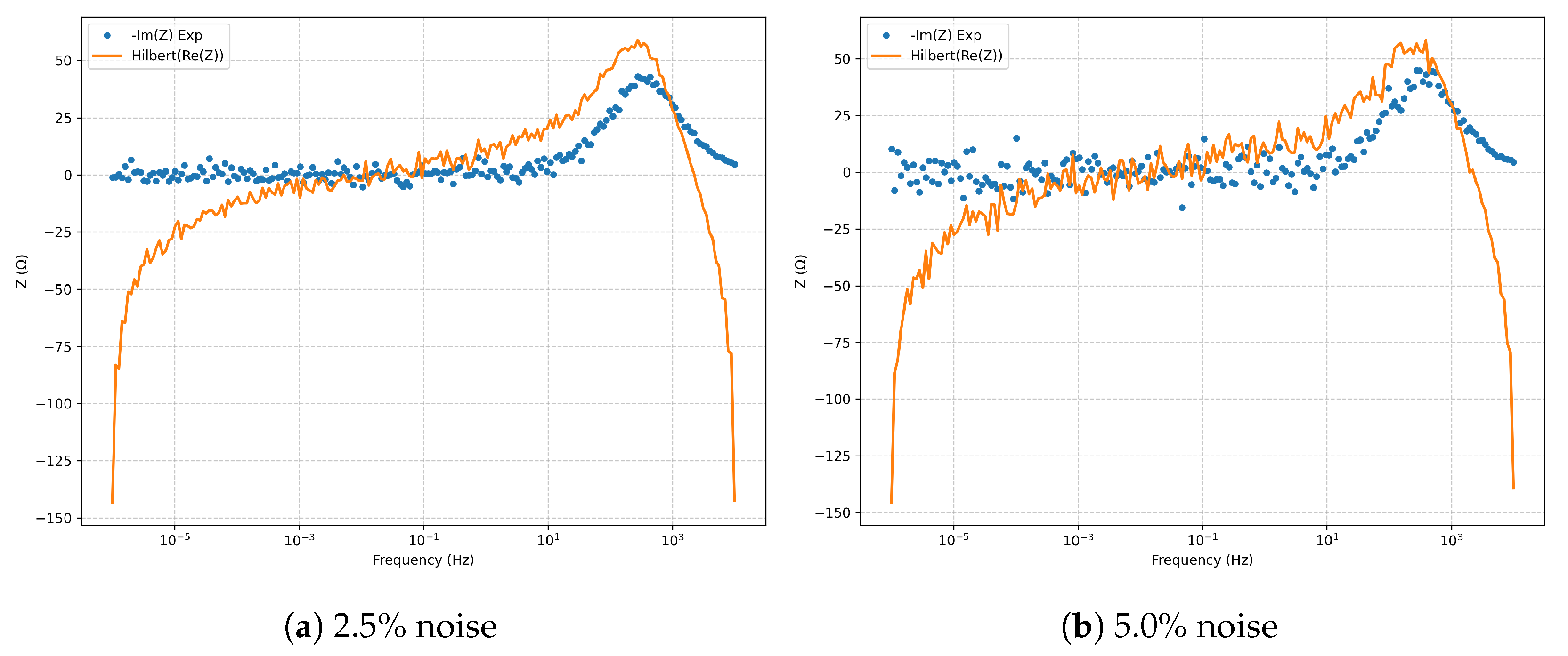
Kramers–Kronig validation via the Hilbert transform (Figure 5) confirms the causality, linearity, and stationarity of the fitted spectra at both noise levels, with no significant violations.
The quantitative summary in Table 1 shows and adjusted values exceeding 0.997 in all cases, with fitted parameters lying within narrow 95% confidence intervals around nominal values. Increasing the noise from to causes modest increases in RMSE, , AIC, and BIC, as well as slight variations in R, L, and C, without compromising the model’s validity.
Overall, the series RLC model demonstrates high stability and predictive reliability under moderate noise, preserving both statistical robustness and physical consistency.
4.1. Model: Classic Randles
The classic Randles model was evaluated under controlled noise levels of and . In both cases, the characteristic semicircle appears slightly depressed due to discrete sampling, while the fit reproduces the experimental trace with high fidelity over several decades of frequency. Figure 6, Figure 7, Figure 8, Figure 9 and Figure 10 present paired panels (left: ; right: ) for the Nyquist diagram, Bode plots (magnitude and phase), complex residuals, and the Kramers–Kronig validation.
In the Nyquist plots (Figure 6), a well-defined semicircle is observed, with a diameter corresponding to . Increasing noise produces only a larger scatter in the high-frequency region, without altering the global morphology. In the Bode plots (Figure 7 and Figure 8), the phase minimum near is accurately captured for both noise levels. The residuals (Figure 9) remain centered and trend-free; at noise, the variance increases without introducing systematic bias. The Kramers–Kronig check (Figure 10) confirms causality and linearity across the full frequency domain.
Quantitatively (Table 2), RMSE increases moderately from 3.2200 at noise to 6.5700 at , while and are maintained in all cases. The estimated parameters fall within the 95% confidence intervals around their nominal values, confirming robust identifiability even under moderate noise.
Overall, these results support the robustness of the classic Randles model for systems dominated by charge-transfer processes and an ideal double-layer capacitance, preserving predictive accuracy and physical consistency under controlled experimental perturbations.
4.2. Model: Randles + CPE
Increasing the noise level from to produces a controlled growth in error (RMSE: 3.3100 → 6.5200) and a moderate decrease in (0.9903 → 0.9634), while preserving spectral agreement (Table 3). The Nyquist diagram retains the characteristic depressed semicircle associated with the CPE (Figure 11), whereas in the Bode plots (Figure 12 and Figure 13) the fit accurately reproduces the magnitude across several decades and precisely locates the phase minimum.
Complex residuals (Figure 14) remain centered and drift-free for both noise levels; the increase in variance at is consistent with the added perturbation. The Kramers–Kronig validation (Figure 15) confirms causality and linearity, with no evidence of nonlinearity or nonstationarity.
Regarding parameters, remains stable and within its 95% confidence intervals (Table 3), while Q and n exhibit the typical collinearity of non-ideal elements (Cond# –). For physical interpretation, the effective capacitance is computed using the Brug correction:
yielding – for , , , and . This corresponds to – and –, in excellent agreement with the experimentally observed phase minimum.
When compared at the same noise level, the classic Randles model is more parsimonious at (lower AIC in Table 2; AIC relative to CPE), whereas at Randles+CPE offers a significant advantage (AIC lower in Table 3; AIC ), capturing non-idealities without overfitting and preserving white residuals.
In summary, Randles+CPE reproduces with high fidelity the depressed arc and fractional phase shift typical of non-ideal interfaces, outperforming the classic Randles model under conditions of pronounced non-ideality or higher noise, while preserving stability under rigorous statistical and physico–mathematical validation (Figure 11, Figure 12, Figure 13, Figure 14 and Figure 15; Table 3).
4.3. Model: Randles + Warburg
The inclusion of the Warburg element introduces a 4.5000 × 101∘ tail in the Nyquist plot (Figure 16) and a slope in the logarithmic magnitude of the Bode plot, accompanied by a phase tending toward at low frequencies (Figure 17 and Figure 18). Both features are consistently observed at and noise levels, supporting the presence of a mass-transport–limiting process.
Increasing the noise level raises the RMSE from 3.1900 to 6.3800 and reduces from 0.9930 to 0.9725 (Table 4), while maintaining close agreement in both Nyquist and Bode domains (Figure 16, Figure 17 and Figure 18). Residuals remain centered and trend-free (Figure 19), and Kramers–Kronig validation confirms causality and linearity (Figure 20), ruling out artifacts from nonlinearity or nonstationarity.
, , and are estimated stably with narrow 95% confidence intervals at both noise levels (Table 4). In contrast, the effective diffusivity shows greater uncertainty, especially at , where the 95% CI reaches the lower bound of the fit (1.0000 × 10⁻⁶–9.4900 × 10⁻⁴). This indicates that, within the available frequency window, the diffusive component is morphologically detectable (Figure 16 and Figure 18) but its magnitude is partially ill-conditioned. Extending the frequency sweep to lower values and/or using a finite-length Warburg variant (e.g., with ) would help constrain .
The phase trend toward (Figure 18) and the tail in the Nyquist plot (Figure 16) are consistent with semi-infinite diffusion of electroactive species to/from the interface. The stability of under noise confirms that the faradaic kinetics are well identified, with the main variation residing in the mass-transport component (Table 4).
Compared to the classic Randles model, adding the Warburg element improves model likelihood at both noise levels (AIC: 349 vs. 362 at ; 348 vs. 353 at ; cf. Table 4 vs. Table 2). This indicates that the diffusive signature adds genuine information without overfitting, consistent with white residuals (Figure 19) and the KK validation (Figure 20).
4.4. Model:
The series combination , placed in parallel with , reproduces an arc with a diffusive tail in the Nyquist plot (Figure 21). In the Bode magnitude representation, the fit accurately follows the simulated data over several frequency decades (Figure 22), while the phase exhibits the expected drift toward the diffusion-controlled regime (approaching at low frequencies; Figure 23). Increasing noise from to barely affects the morphological agreement, with discrepancies mainly concentrated at high frequencies, where the capacitive pathway of dominates.
The RMSE increases from 3.3300 to 6.4700, and decreases from 0.9923 to 0.9717 (Table 5), while maintaining close agreement with the reference spectrum. The residuals (real and imaginary parts) remain centered without any trend (Figure 24), and the Kramers–Kronig (Hilbert transform) validation confirms causality and linearity of the simulated spectrum at both noise levels (Figure 25).
The parameters , , and are stable and have narrow 95% confidence intervals (Table 5). The diffusive amplitude is the least constrained: at noise it exhibits a wide 95% CI , and at it reaches the lower bound of the fit . This indicates that, within the available frequency window, the diffusive signature is visible (Figure 21 and Figure 23), but its amplitude is partially ill-conditioned due to the capacitive shunt. The condition number is moderate (), significantly better than in CPE-based models, supporting the overall numerical stability of the fit.
The parallel arrangement with shunts the faradaic branch at high frequencies (almost purely capacitive trajectories), while at low frequencies dominates, producing the 4.5000 × 101∘ diffusive tail (Figure 21 and Figure 23). The constancy of under noise suggests that the interfacial kinetics are well-identified, with the main uncertainty arising from the effective mass transport term encapsulated in .
At noise, this model is less statistically supported than Randles+Warburg and Randles+CPE (AIC = 382 vs. 349 and 370; AIC = +33 and +12, respectively), and even less than the classical Randles (362; AIC = +20). At , its performance approaches that of the classical Randles (354 vs. 353; AIC = +1), but remains below Randles+Warburg (348; AIC = +6) and particularly Randles+CPE (334; AIC = +20). Overall, the statistical evidence favors alternative descriptions when the available frequency window does not sufficiently constrain .
The topology captures the expected kinetic–diffusive interaction and produces physically consistent fits (Figure 21, Figure 22, Figure 23, Figure 24 and Figure 25); however, under the current measurement window its informational advantage is limited compared to Randles+Warburg or Randles+CPE, due to the poor constraint on .
4.5. Model:
This topology combines semi-infinite diffusion () with a non-ideal capacitive response (CPE). In the Nyquist plot, a depressed arc appears along with a diffusive extension at low frequencies (Figure 26); in the Bode magnitude plot, the fit reproduces the spectrum across several decades (Figure 27) and captures the fractional phase minimum associated with (Figure 28).
Increasing the noise from to raises the RMSE from 3.29 to 6.44 and reduces from 0.9904 to 0.9645 (Table 6), while preserving morphological agreement in both representations. The residuals remain centered and trend-free (Figure 29); the Kramers–Kronig test confirms causality and linearity of the spectrum (Figure 30).
The parameters and are stable with narrow 95% confidence intervals at both noise levels (Table 6). The exponent indicates a distribution of relaxation times consistent with interfacial heterogeneity/roughness; – corresponds to an effective capacitance of – (using Brug’s correction, as in the CPE subsection). The diffusive amplitude is the least constrained at noise (95% CI reaches the lower bound), but is better defined at . The condition number is moderate (), much lower than for models with CPE only, suggesting reduced collinearity between () and the diffusive branch when is present.
The CPE accounts for interfacial non-idealities (distribution of time constants), while captures mass-transport control at low frequencies. The phase transition toward (Figure 28) and the Nyquist tail (Figure 26) highlight the diffusive contribution; the stability of supports a well-identified faradaic kinetics.
At noise, this model markedly outperforms the classical Randles (AIC 352 vs. 362; AIC = ) and Randles+CPE (352 vs. 370; ), and is close to Randles+Warburg (352 vs. 349; ). At , it becomes the best-performing alternative among those considered (AIC 333), surpassing Randles+CPE (334), Randles+Warburg (348), and the classical Randles (353) (Table 6 and related tables). This suggests that when interfacial non-ideality and a diffusive component are present simultaneously, the architecture offers the best balance between fit quality and parsimony.
The combination of CPE and Warburg in parallel with provides a coherent and statistically preferred representation of systems exhibiting concurrent interfacial non-ideality and diffusion, with white residuals and consistent KK validation (Figure 26, Figure 27, Figure 28, Figure 29 and Figure 30; Table 6).
4.6. Model: Full Randles
The model reliably reproduces the canonical features: a depressed semicircle at intermediate frequencies and a diffusive tail at low frequencies (Nyquist, Figure 31); magnitude decay around the characteristic frequency and a fractional phase minimum due to the CPE (Figure 32 and Figure 33). The Kramers–Kronig validation shows overall agreement between the spectrum and the Hilbert reconstruction (Figure 35), with bounded deviations at the band edges attributable to the spectral window width.
When increasing noise from to , the RMSE rises from 3.2700 to 6.6200 and decreases from 0.9905 to 0.9625 (Table 7), but the fit morphology remains consistent in both representations (Figure 31, Figure 32 and Figure 33). Residuals remain centered and free from systematic trends; only their variance increases, in line with the noise level (Figure 34).
Figure 34.
Residuals (real and imaginary parts) for the full Randles model.
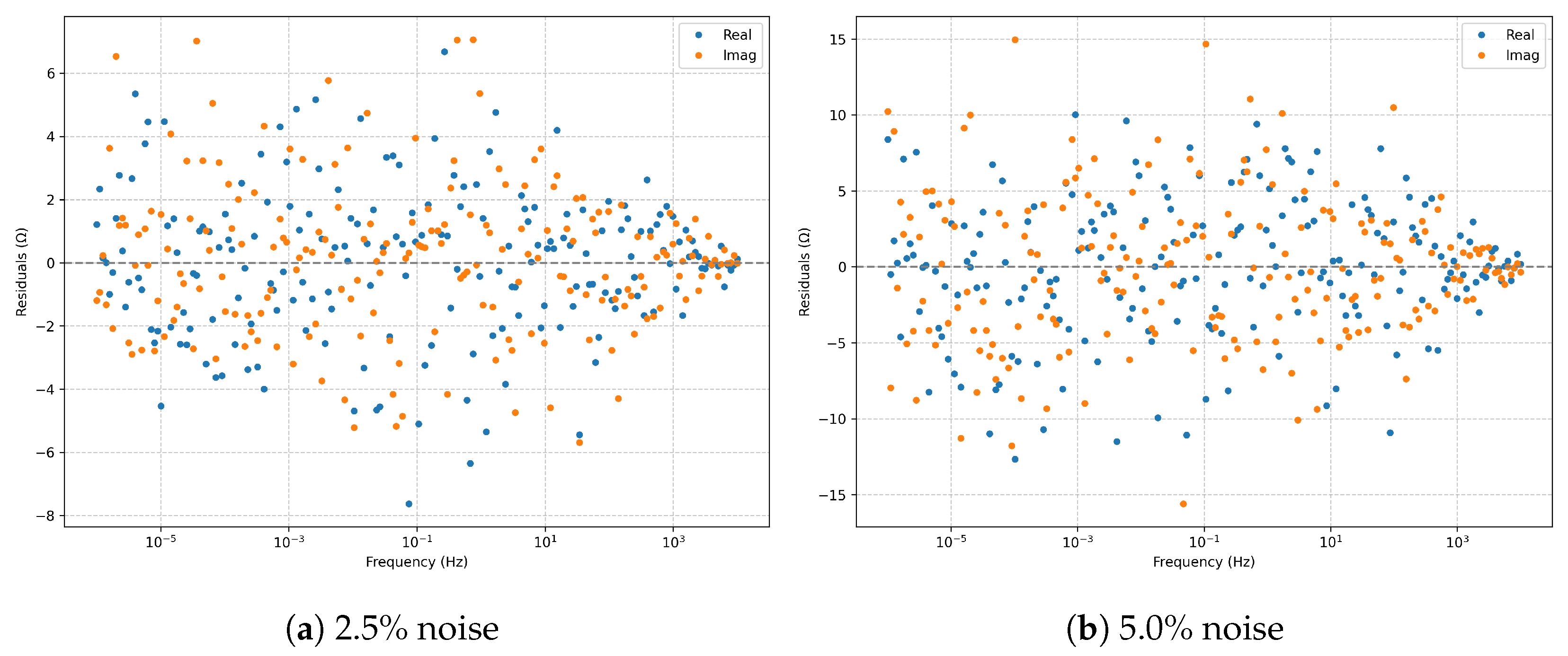
Figure 35.
Kramers–Kronig (Hilbert transform) validation for the full Randles model.
Ohmic and kinetic parameters remain stable (narrow 95% CIs in and ; Table 7). In contrast, Q, n and, particularly, the effective diffusivity exhibit marked collinearity (Cond# ), with reaching the upper bound of the interval at . This indicates that, with the available frequency range, CPE–Warburg separation is not fully excited: the CPE absorbs part of the diffusive curvature and vice versa. A practical way to convey the capacitive response is to report, along with Q and n, the effective capacitance (Brug correction), which here is on the order of a few , consistent with the position of the phase minimum (Figure 33).
The exponent reflects a distribution of times associated with interfacial roughness/heterogeneity, while the tail and magnitude slope corroborate a mass transport component (Warburg). The stability of at both noise levels suggests a well-identified faradaic kinetics, decoupled from the uncertainties in Q, n and (Table 7).
At , the AIC of the full Randles (350) is comparable to Randles+Warburg (349) and better than Randles+CPE (370), but does not provide a material advantage over the option without CPE or without Warburg (Figure 31, Figure 32 and Figure 33; Table 7). At the model is penalized for complexity (AIC 356; BIC 376) compared to more parsimonious alternatives, especially and Randles+CPE, which achieve lower AIC values with equal or better fidelity. Consequently, if σ is poorly bounded and the AIC improvement is marginal, the full version is not statistically justified.
The full Randles simultaneously captures interfacial non-ideality and diffusion, but with the present spectral range, the gain over partial models is limited and the identifiability of is fragile. For data with mild non-ideality and moderate diffusion, or Randles+Warburg offer a superior trade-off between physical realism and parsimony; the full model should be reserved for spectra with clear and quantifiable evidence of both contributions (Figure 31, Figure 32, Figure 33, Figure 34 and Figure 35; Table 7).
4.7. Global Model Comparison
Table 8 summarizes the key fitting metrics for all seven evaluated models at both noise levels. At , differences in RMSE among the more complex models (Randles full, Randles+Warburg, ) are marginal, with statistical improvements in AIC and BIC insufficient to justify overparameterization when or n exhibit broad confidence intervals or strong collinearity. At noise, the more parsimonious models (Randles+CPE and ) yield lower AIC/BIC values with negligible loss, reflecting greater robustness against signal degradation.
From a physical standpoint, the simultaneous inclusion of a CPE and Warburg impedance (Randles full) is warranted only when the spectrum exhibits quantifiable evidence of both interfacial non-ideality and semi-infinite diffusion, and when the spectral range adequately excites both processes. In the absence of these conditions, partial models offer a superior trade-off between fitting fidelity, parameter stability, and parsimony.
5. Conclusions
This work establishes a fully integrated and analytically rigorous framework for Electrochemical Impedance Spectroscopy (EIS) analysis, combining exact impedance formulations, closed-form Jacobians, hybrid global–local optimization, and exhaustive statistical validation. Applied consistently across seven representative equivalent circuit models under controlled synthetic conditions, the methodology delineates precise statistical and physical boundaries for model applicability, bridging the gap between theoretical formulation and practical implementation.
Results demonstrate that the classical Randles circuit remains the most parsimonious and statistically optimal choice for systems with ideal charge-transfer kinetics and capacitive behavior, while configurations incorporating Constant Phase Elements (CPE) and Warburg diffusion elements provide superior fidelity for heterogeneous or diffusion-limited interfaces. The robustness of estimation across noise levels, alongside the ability to quantify non-ideal capacitive parameters and diffusive amplitudes, underscores the stability and reproducibility of the approach.
Critically, automated Kramers–Kronig compliance testing ensures that all fitted spectra satisfy the fundamental principles of linearity and causality, eliminating a recurrent source of interpretative bias in EIS literature. The modularity of the platform enables rapid extension to novel circuit topologies, integration with experimental datasets, and coupling with advanced electrochemical–transport models.
By uniting analytical precision, computational efficiency, and rigorous statistical scrutiny, this framework delivers an unprecedented level of objectivity in EIS model selection and parameter interpretation. As such, it is positioned to become a reference standard for quantitative EIS analysis, setting a reproducible benchmark for the accurate characterization and optimization of electrochemical systems in energy storage, corrosion science, and electrocatalysis. .
Author Contributions
Conceptualization, F.A.N.P.; methodology, F.A.N.P.; software, F.A.N.P.; validation, F.A.N.P.; formal analysis, F.A.N.P.; investigation, F.A.N.P.; resources, F.A.N.P.; data curation, F.A.N.P.; writing—original draft preparation, F.A.N.P.; writing—review and editing, F.A.N.P.; visualization, F.A.N.P.; supervision, F.A.N.P.; project administration, F.A.N.P. The author has read and agreed to the published version of the manuscript.
Funding
This research received no external funding. The APC was funded by Universidad Politécnica de Lázaro Cárdenas (UPLC), Michoacán, Mexico.
Institutional Review Board Statement
Not applicable.
Informed Consent Statement
Not applicable.
Data Availability Statement
The datasets and code are available from the corresponding author on reasonable request.
Acknowledgments
I sincerely appreciate the Universidad Politécnica de Lázaro Cárdenas for offering me the opportunity and the essential resources to carry out this project.
Conflicts of Interest
The author declares no conflicts of interest.
Abbreviations
The following abbreviations are used in this manuscript:
| AIC | Akaike Information Criterion |
| BIC | Bayesian Information Criterion |
| CI | Confidence interval |
| CPE | Constant-phase element |
| DE | Differential Evolution |
| DRT | Distribution of relaxation times |
| ECM | Equivalent circuit model |
| EIS | Electrochemical impedance spectroscopy |
| KK | Kramers–Kronig |
| LM | Levenberg–Marquardt |
| LTI | Linear time-invariant |
| RMSE | Root-mean-square error |
| RLC | Resistor–Inductor–Capacitor |
| Solution resistance | |
| Charge-transfer resistance | |
| Double-layer capacitance | |
| Warburg (semi-infinite diffusion) impedance |
References
- Magar, H. S., Hassan, R. Y., & Mulchandani, A. (2021). Electrochemical impedance spectroscopy (EIS): Principles, construction, and biosensing applications. Sensors, 21(19), 6578. [CrossRef]
- Lazanas, A. C., & Prodromidis, M. I. (2023). Electrochemical impedance spectroscopy—A tutorial. ACS Measurement Science Au, 3(3), 162–193. [CrossRef]
- Perry, D., & Mamlouk, M. (2021). Probing mass transport processes in Li-ion batteries using electrochemical impedance spectroscopy. Journal of Power Sources, 514, 230577. [CrossRef]
- Harrington, D. A., & Van den Driessche, P. (2011). Mechanism and equivalent circuits in electrochemical impedance spectroscopy. Electrochimica Acta, 56, 8005–8013. [CrossRef]
- Maksoud, M. A., Bekhit, M., Waly, A. L., & Awed, A. S. (2023). Optical and dielectric properties of polymer nanocomposite based on PVC matrix and Cu/Cu2O nanorods synthesized by gamma irradiation for energy storage applications. Physica E: Low-dimensional Systems and Nanostructures, 148, 115661. [CrossRef]
- Van Haeverbeke, M., Stock, M., & De Baets, B. (2022). Equivalent electrical circuits and their use across electrochemical impedance spectroscopy application domains. IEEE Access, 10, 51363–51379. [CrossRef]
- Gateman, S. M., Gharbi, O., De Melo, H. G., Ngo, K., Turmine, M., & Vivier, V. (2022). On the use of a constant phase element (CPE) in electrochemistry. Current Opinion in Electrochemistry, 36, 101133. [CrossRef]
- Randviir, E. P., & Banks, C. E. (2022). A review of electrochemical impedance spectroscopy for bioanalytical sensors. Analytical Methods, 14(45), 4602–4624. [CrossRef]
- Esser, M., Rohde, G., & Rehtanz, C. (2022). Electrochemical impedance spectroscopy setup based on standard measurement equipment. Journal of Power Sources, 544, 231869. [CrossRef]
- Barbero, G., Batalioto, F., Figueiredo Neto, A. M., & Lelidis, I. (2021). Deviations from linearity in impedance spectroscopy measurements confirmed by Kramers–Kronig analysis. Electrochimica Acta, 388, 139277. [CrossRef]
- Zhang, R., Black, R., Sur, D., Karimi, P., Li, K., DeCost, B., & Hattrick-Simpers, J. (2023). Editors’ choice—AutoEIS: Automated Bayesian model selection and analysis for electrochemical impedance spectroscopy. Journal of The Electrochemical Society, 170(8), 086502. [CrossRef]
- Nuñez Pérez, F. A. (2024). Electrochemical analysis of corrosion resistance of manganese-coated annealed steel: Chronoamperometric and voltammetric study. AppliedChem, 4(4), 367–383. [CrossRef]
- Núñez-Pérez, F. A. (2024). Electrochemical analysis of the corrosion resistance of annealed steel with nickel coating in marine environment simulations: Chronoamperometric and voltammetric study. Ibero-American Journal of Engineering & Technology Studies, 4(1), 62–70. [CrossRef]
- Davey, S. B., Cameron, A. P., Latham, K. G., & Donne, S. W. (2021). Combined step potential electrochemical spectroscopy and electrochemical impedance spectroscopy analysis of the glassy carbon electrode in an aqueous electrolyte. Electrochimica Acta, 396, 139220. [CrossRef]
- Chen, C.-C., Hung, C.-H., Zhu, H.-X., & Chen, J.-Z. (2024). High-sensitivity electrical admittance sensor with regression analysis for measuring mixed electrolyte concentrations. Sensors, 24(22), 7379. [CrossRef]
- López-Villanueva, J. A., & Rodríguez Bolívar, S. (2022). Constant phase element in the time domain: The problem of initialization. Energies, 15(3), 792. [CrossRef]
- Wang, L., Song, Z., Zhu, L., & Jiang, J. (2023). Fast electrochemical impedance spectroscopy of lithium-ion batteries based on the large square wave excitation signal. iScience, 26(4), 106531. [CrossRef]
- Caeiro, A., Canhoto, J., & Rocha, P. R. (2025). Electrochemical impedance spectroscopy as a micropropagation monitoring tool for plants: A case study of tamarillo (Solanum betaceum) callus. iScience, 28(2), 109123. [CrossRef]
- Berliner, M. D., Jiang, B., Cogswell, D. A., Bazant, M. Z., & Braatz, R. D. (2022). Novel operating modes for the charging of lithium-ion batteries. Journal of The Electrochemical Society, 169(10), 100546. [CrossRef]
- Suárez-Herrera, M. F., & Scanlon, M. D. (2019). On the non-ideal behaviour of polarised liquid–liquid interfaces. Electrochimica Acta, 328, 135110. [CrossRef]
- Silva, T. R., Araújo, A. J. M., Raimundo, R. A., Ferreira, L. S., Macedo, D. A., Marques, P. A. A. P., Loureiro, F. J. A., & Fagg, D. P. (2026). One-step fabrication of self-supported MnCo2O4-reduced graphene oxide-based anodes for the alkaline oxygen evolution reaction. Journal of Physics and Chemistry of Solids, 208, 113067. [CrossRef]
- Ammar, N., & Vincent, D. (2020). Design and analysis of two layers RLC network of rectangular topology by wave concept iterative process method. International Journal of Numerical Modelling: Electronic Networks, Devices and Fields, 33(6), e2805. [CrossRef]
- Schalenbach, M., Raijmakers, L., Tempel, H., & Eichel, R. A. (2025). How microstructures, oxide layers, and charge transfer reactions influence double layer capacitances. Part 2: Equivalent circuit models. Electrochemical Science Advances, 5(1), e202400010. [CrossRef]
- Patel, B., Sorrentino, A., & Vidakovic-Koch, T. (2025). Data-driven analysis of electrochemical impedance spectroscopy using the Loewner framework. iScience, 28(3), 109987. [CrossRef]
- Orazem, M. E., & Ulgut, B. (2024). On the proper use of a Warburg impedance. Journal of The Electrochemical Society, 171(4), 040526. [CrossRef]
- van den Bergh, W., & Stefik, M. (2022). Understanding rapid intercalation materials one parameter at a time. Advanced Functional Materials, 32(31), 2204126. [CrossRef]
Figure 1.
Nyquist diagrams for the series RLC model: comparison between and noise.

Figure 2.
Bode magnitude for the series RLC model at and noise.
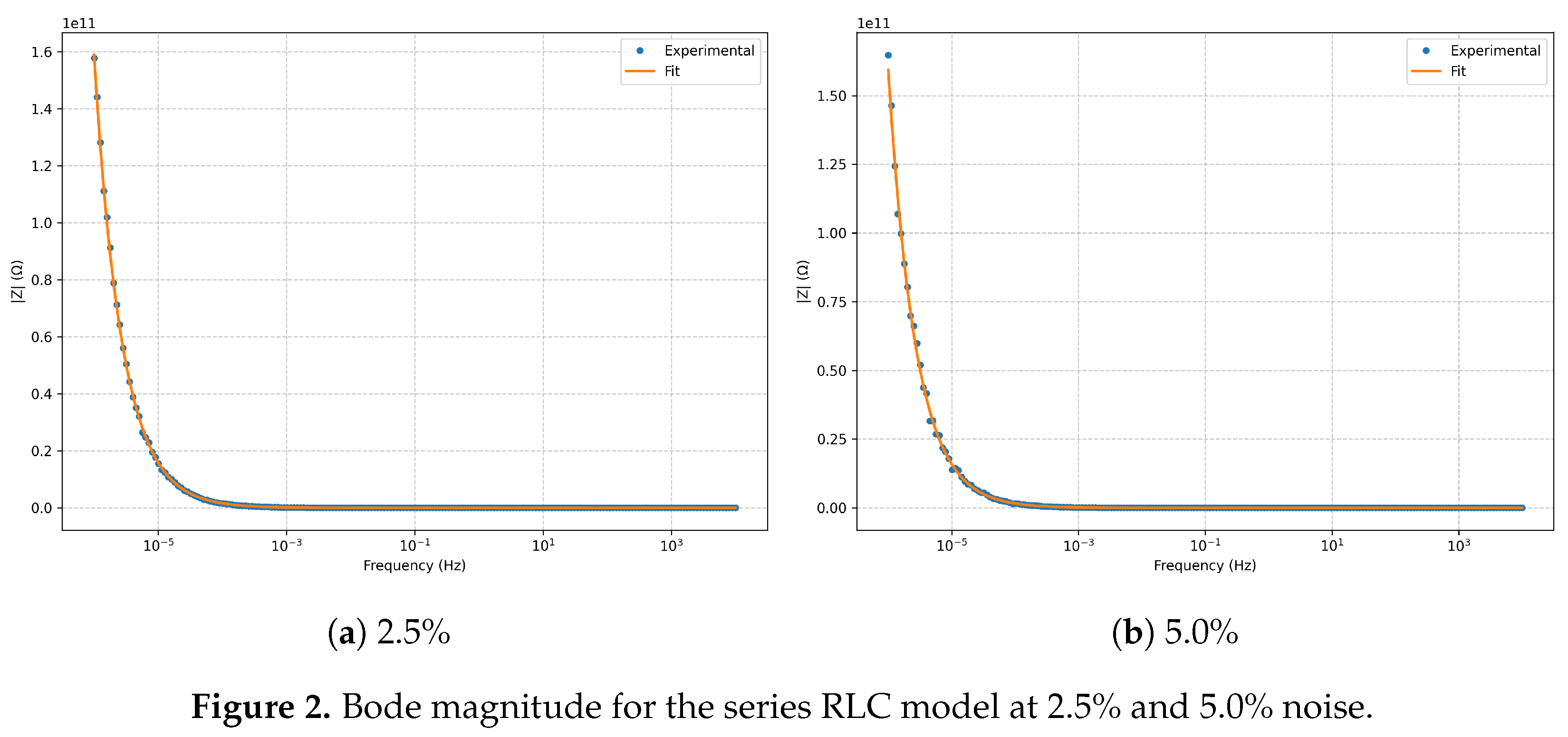
Figure 3.
Bode phase for the series RLC model at and noise.
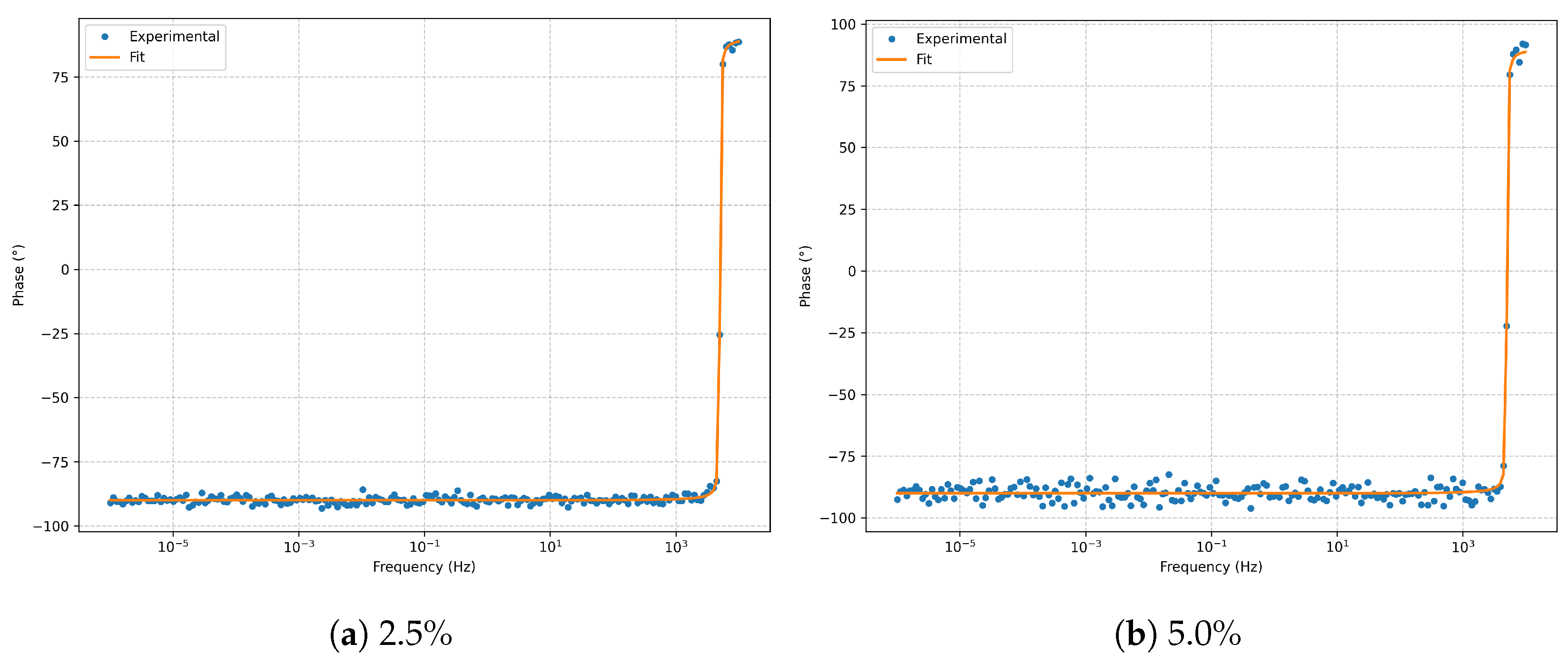
Figure 4.
Residuals (real and imaginary parts) for the series RLC model.
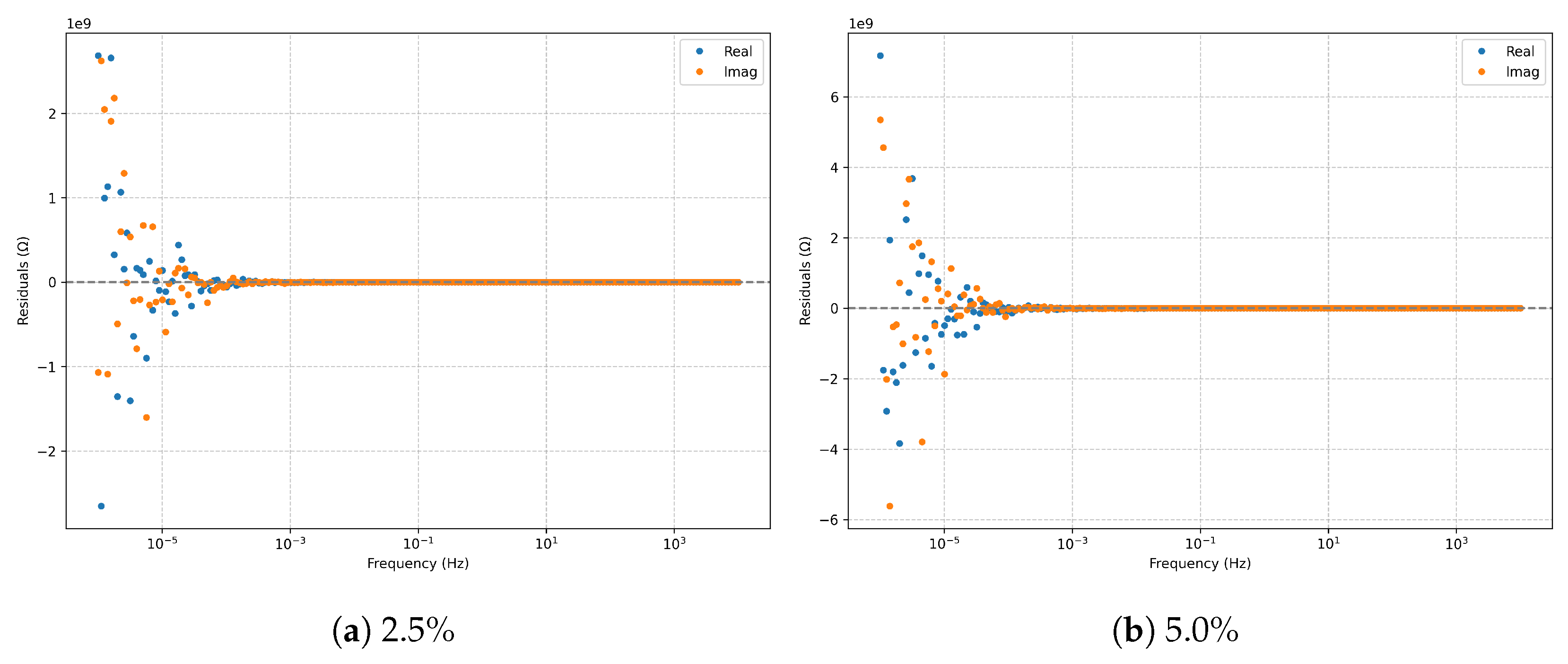
Figure 5.
Kramers–Kronig validation (Hilbert transform) for the series RLC model.
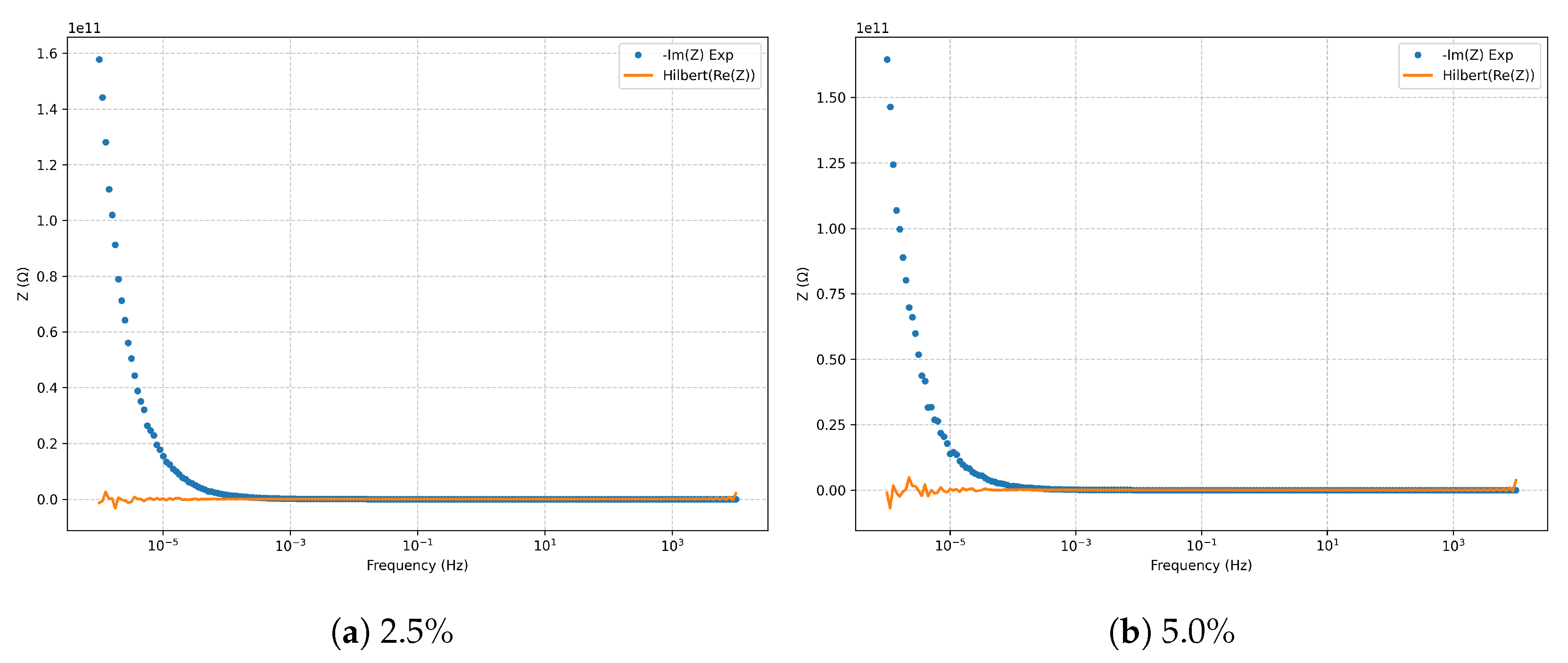
Figure 6.
Nyquist diagrams for the classic Randles model: comparison between 2.5% and 5.0% noise levels.
Figure 6.
Nyquist diagrams for the classic Randles model: comparison between 2.5% and 5.0% noise levels.
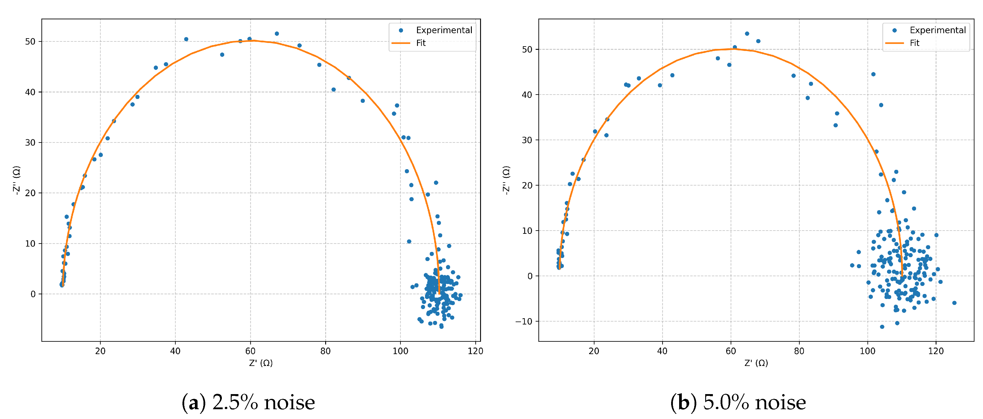
Figure 7.
Bode magnitude for the classic Randles model at 2.5% and 5.0% noise levels.
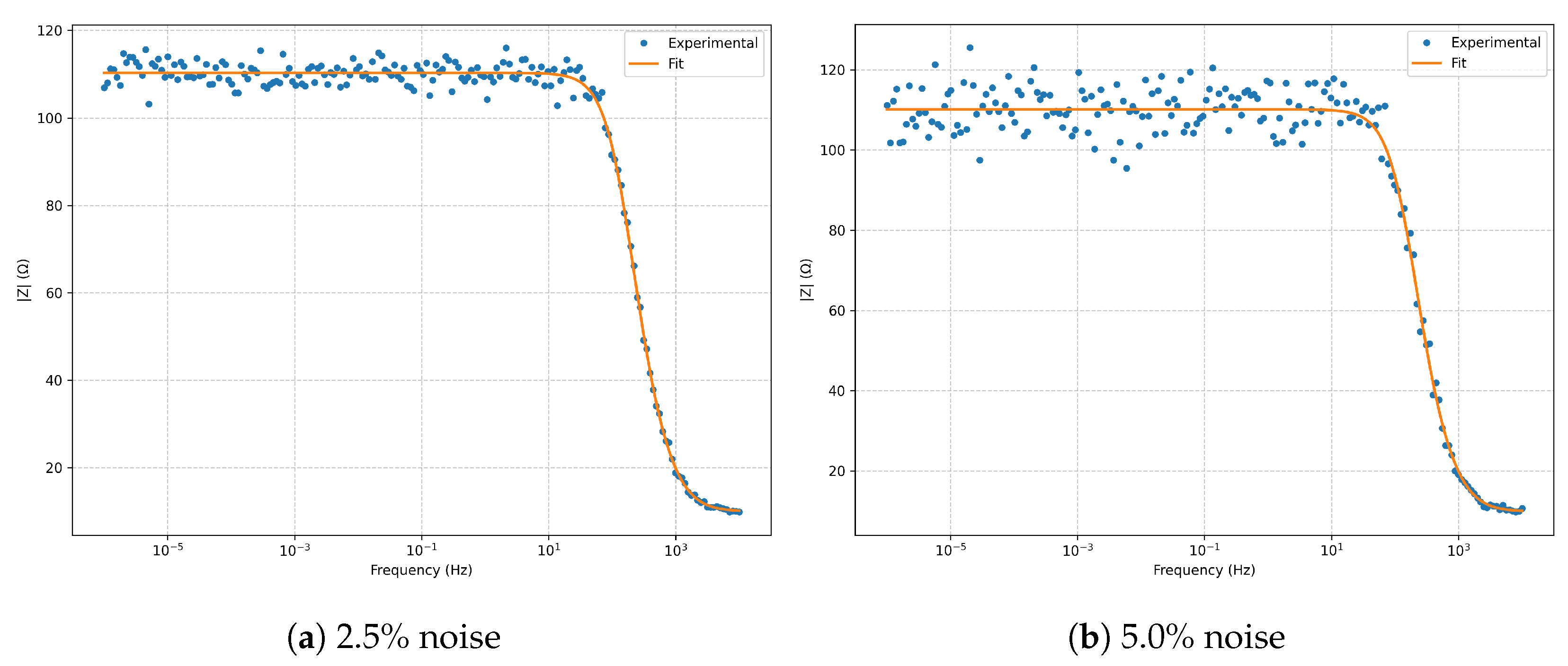
Figure 8.
Bode phase for the classic Randles model at 2.5% and 5.0% noise levels.
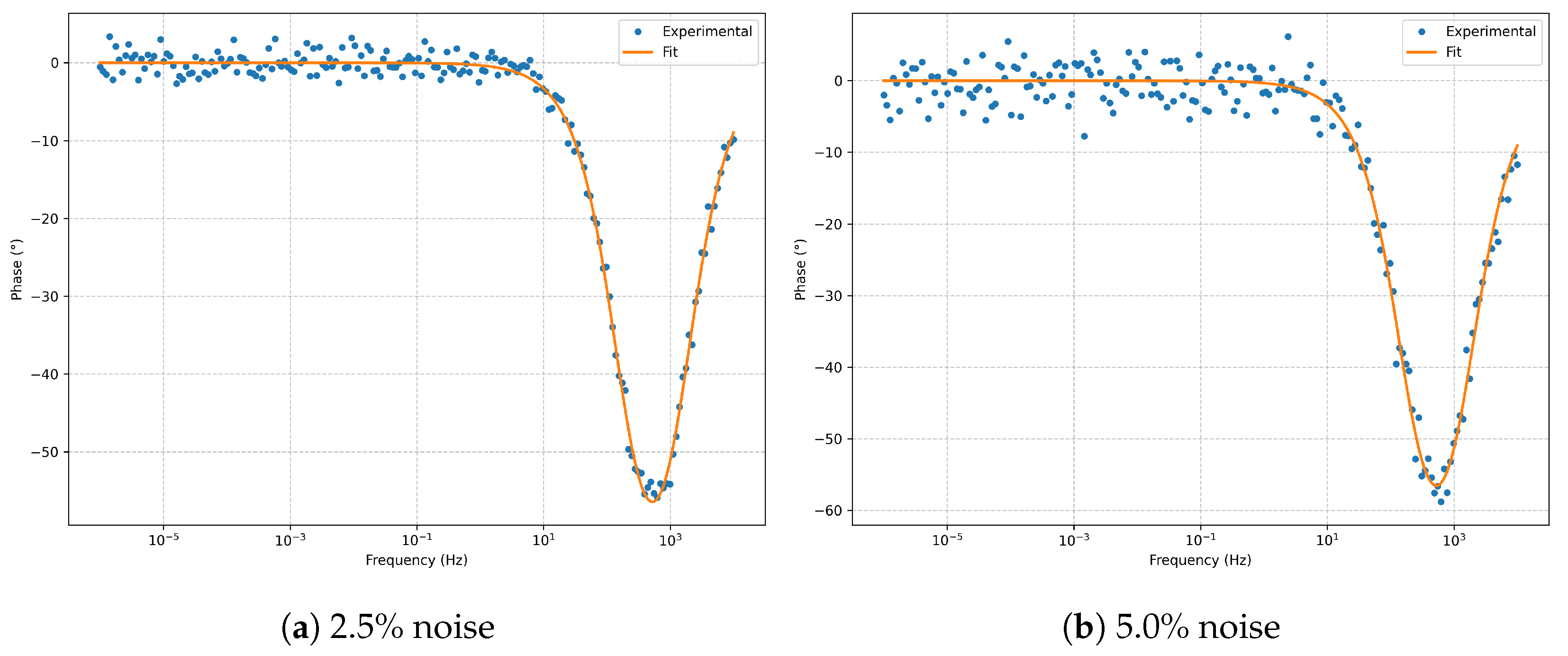
Figure 9.
Residuals (real and imaginary parts) for the classic Randles model.
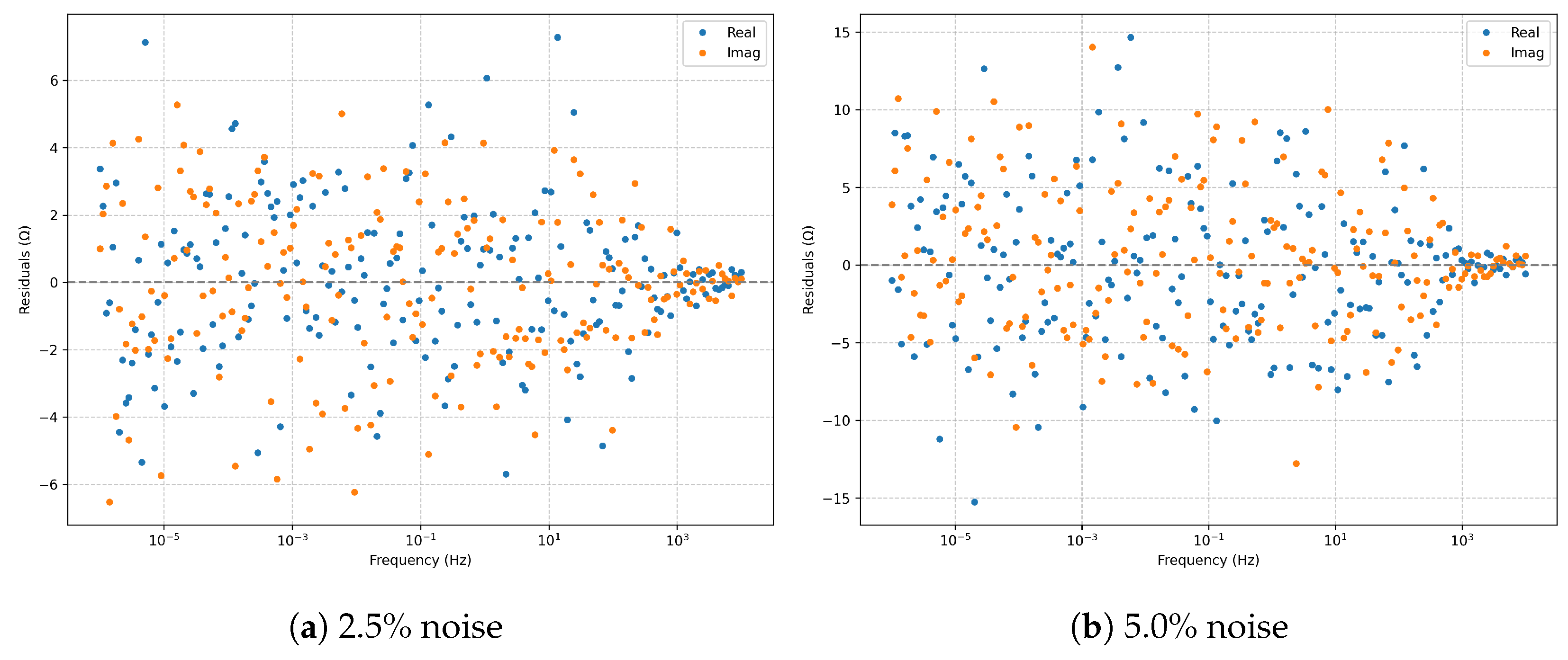
Figure 10.
Kramers–Kronig validation (Hilbert transform) for the classic Randles model.
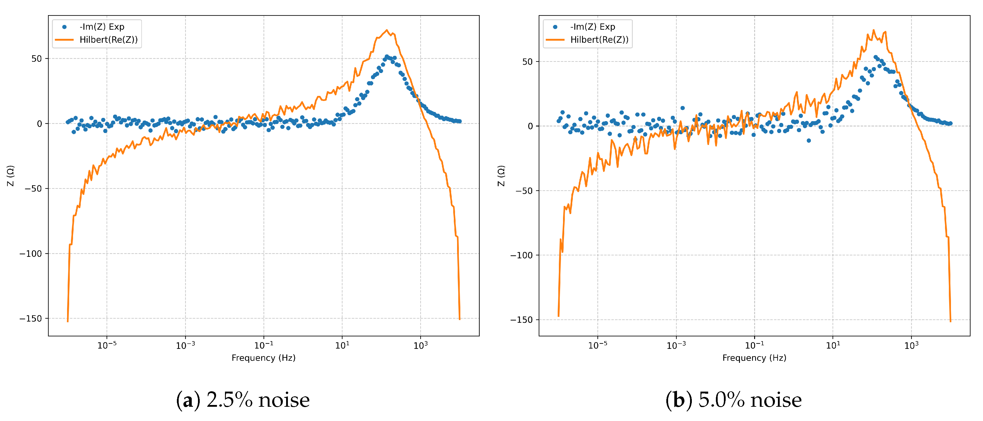
Figure 11.
Nyquist diagrams for the Randles+CPE model: comparison between 2.5% and 5.0% noise levels.
Figure 11.
Nyquist diagrams for the Randles+CPE model: comparison between 2.5% and 5.0% noise levels.
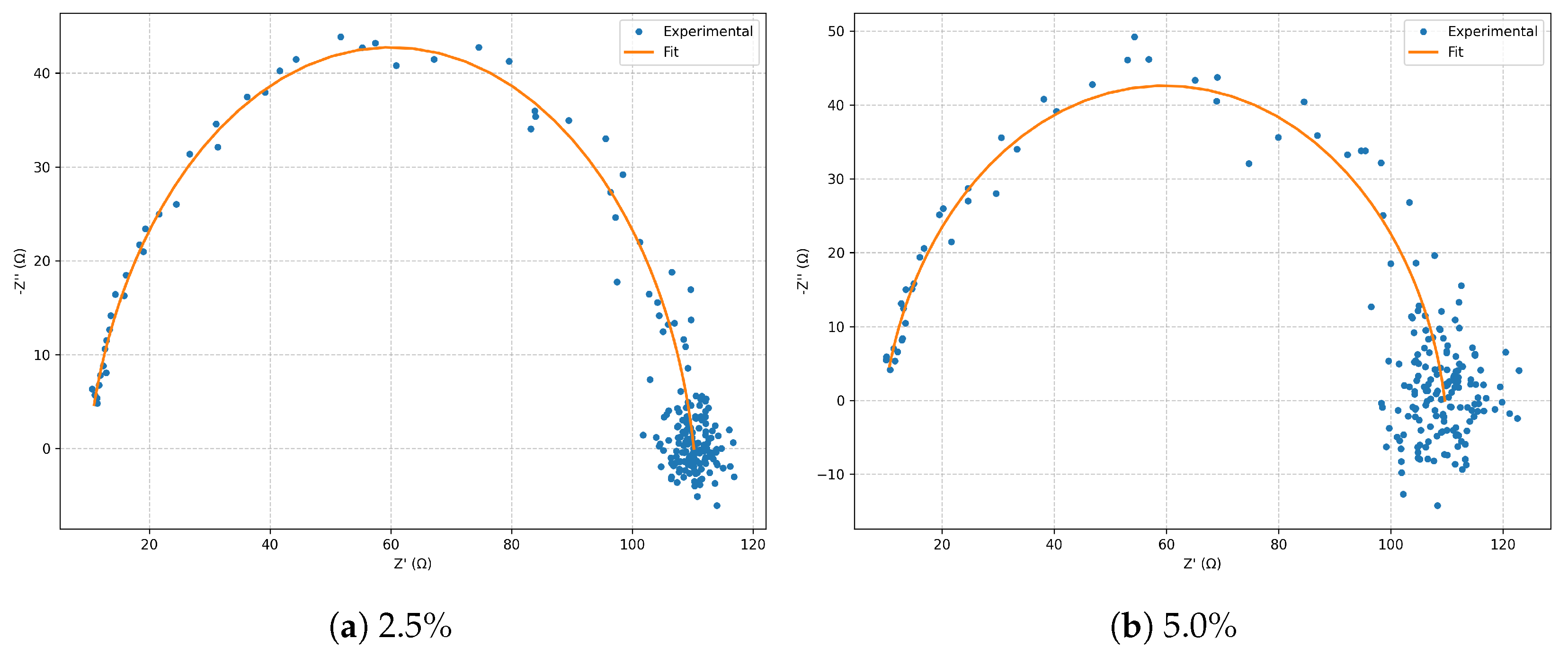
Figure 12.
Bode magnitude for the Randles+CPE model at 2.5% and 5.0% noise levels.
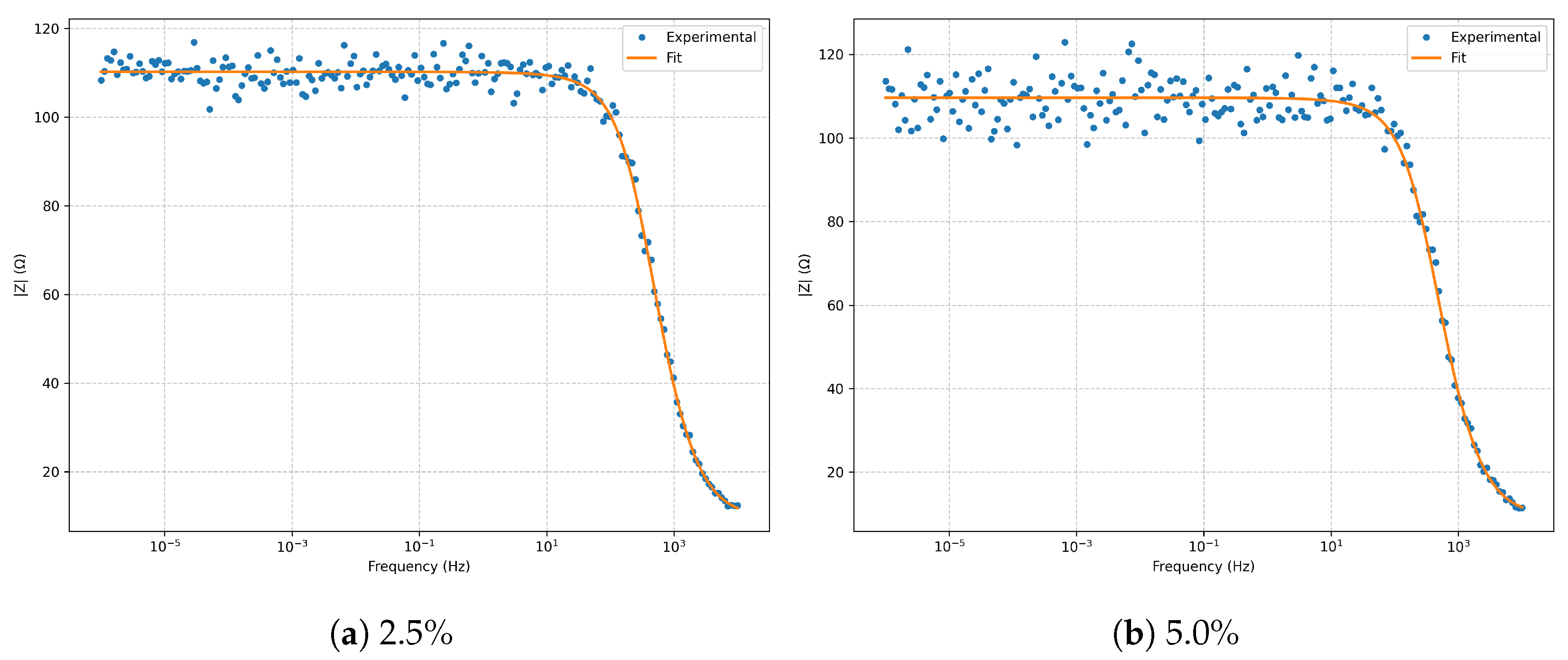
Figure 13.
Bode phase for the Randles+CPE model at 2.5% and 5.0% noise levels.
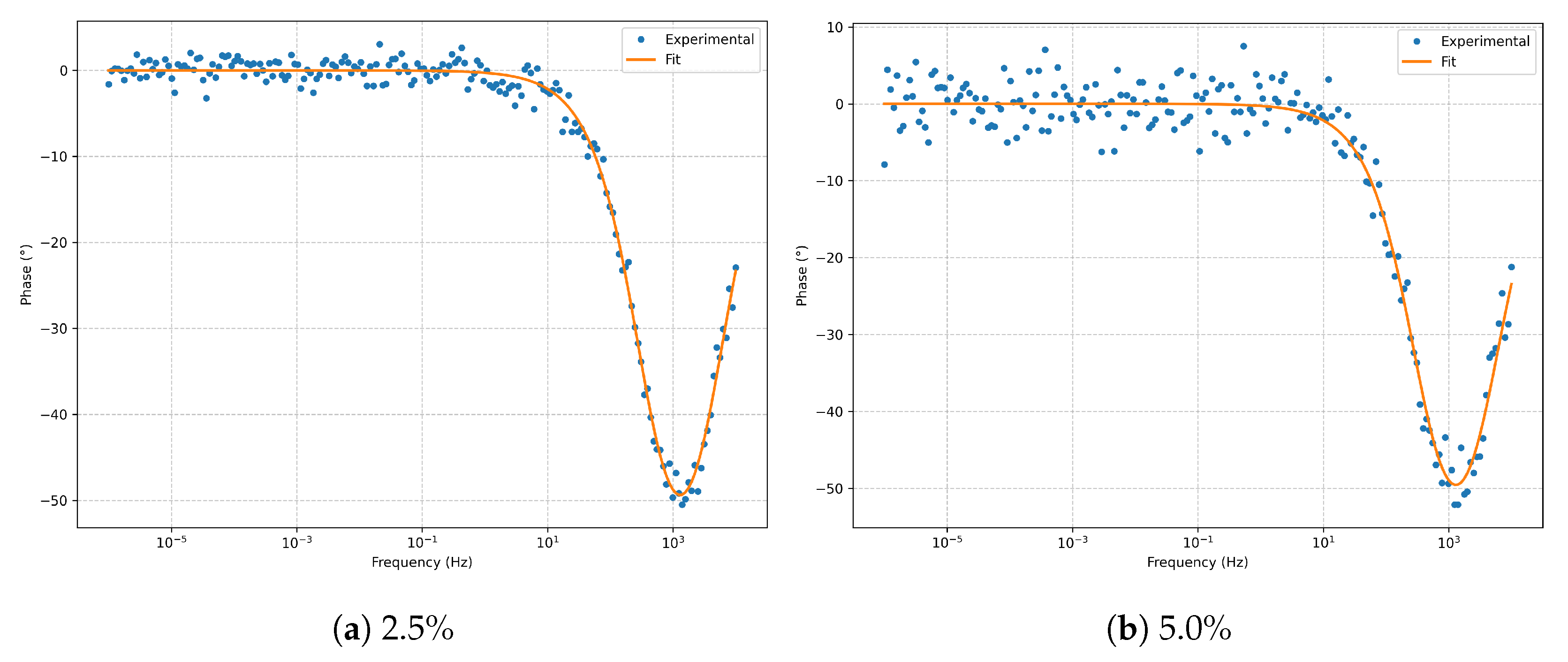
Figure 14.
Complex residuals (real and imaginary parts) for the Randles+CPE model.
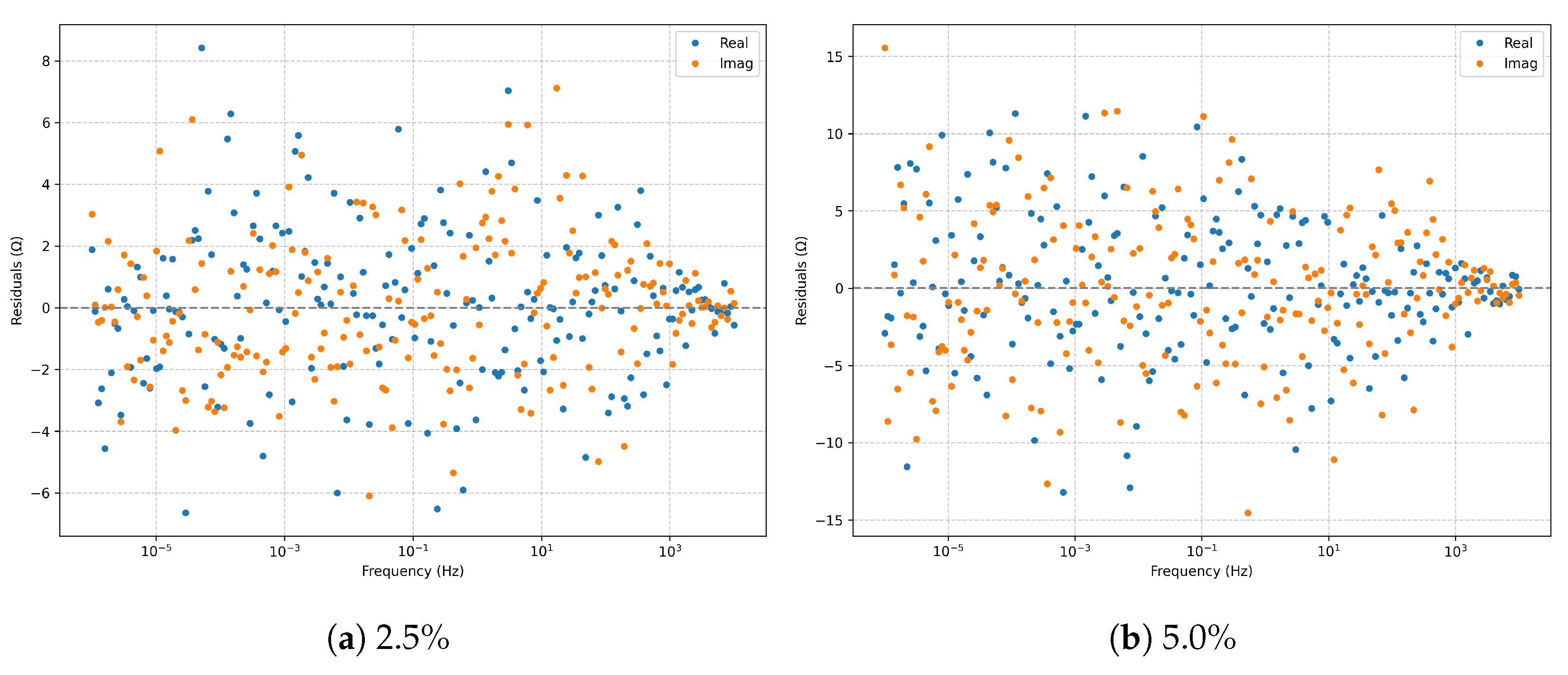
Figure 15.
Kramers–Kronig validation (Hilbert transform) for the Randles+CPE model.
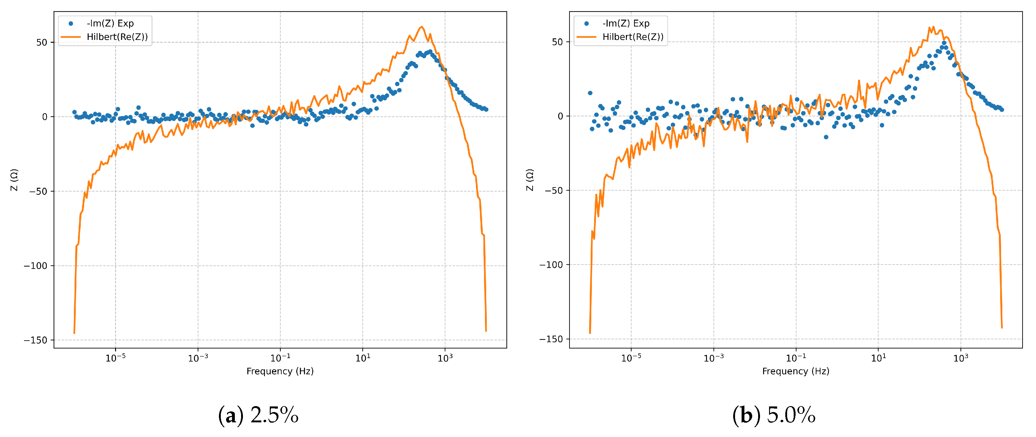
Figure 16.
Nyquist diagrams for the Randles+Warburg model: comparison between 2.5% and 5.0% noise levels.
Figure 16.
Nyquist diagrams for the Randles+Warburg model: comparison between 2.5% and 5.0% noise levels.
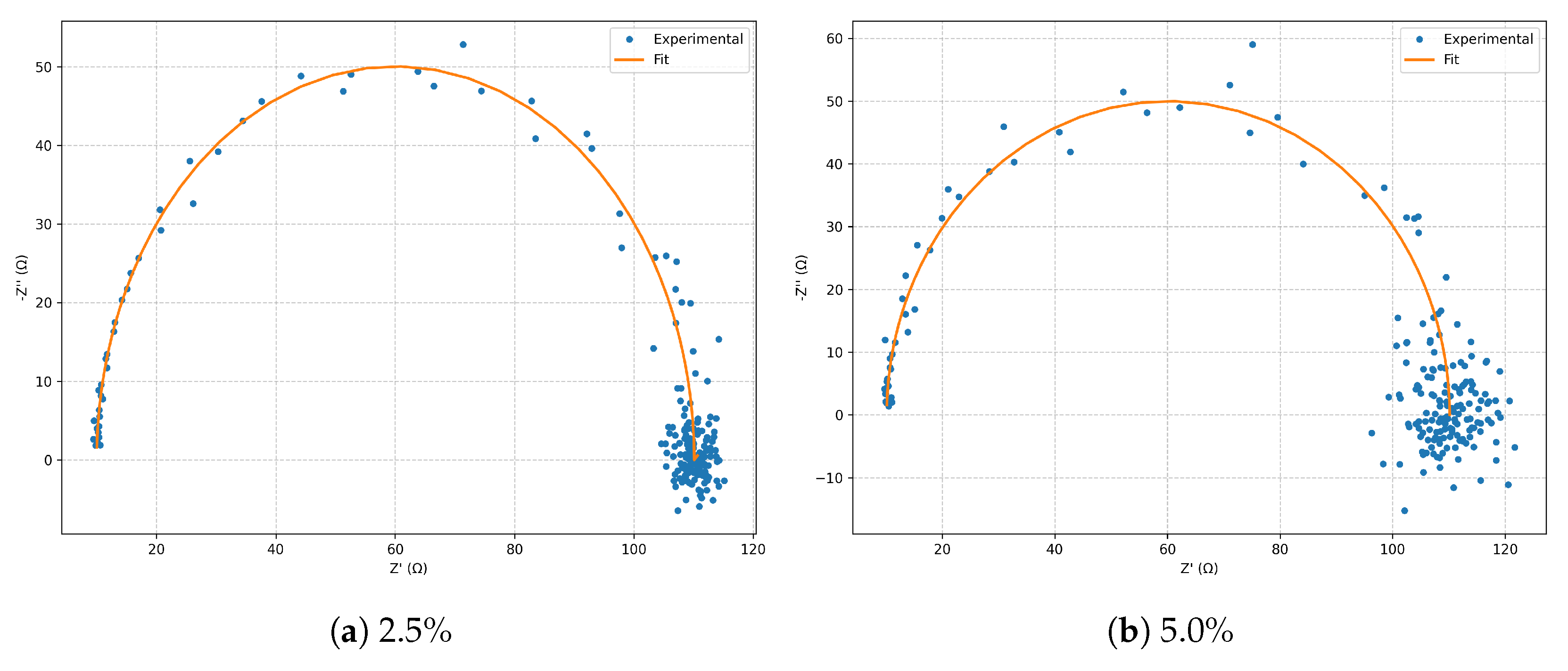
Figure 17.
Bode magnitude plots for the Randles+Warburg model at 2.5% and 5.0% noise levels.
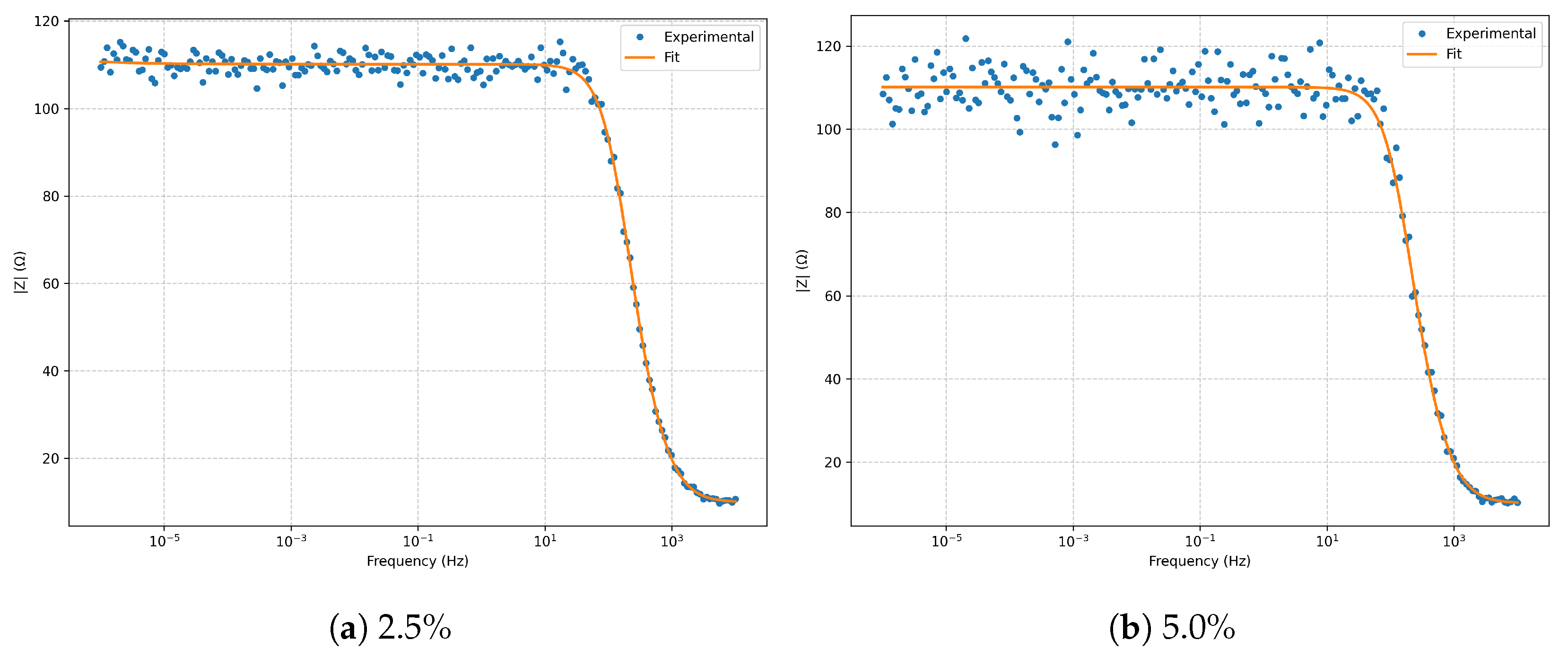
Figure 18.
Bode phase plots for the Randles+Warburg model at 2.5% and 5.0% noise levels.
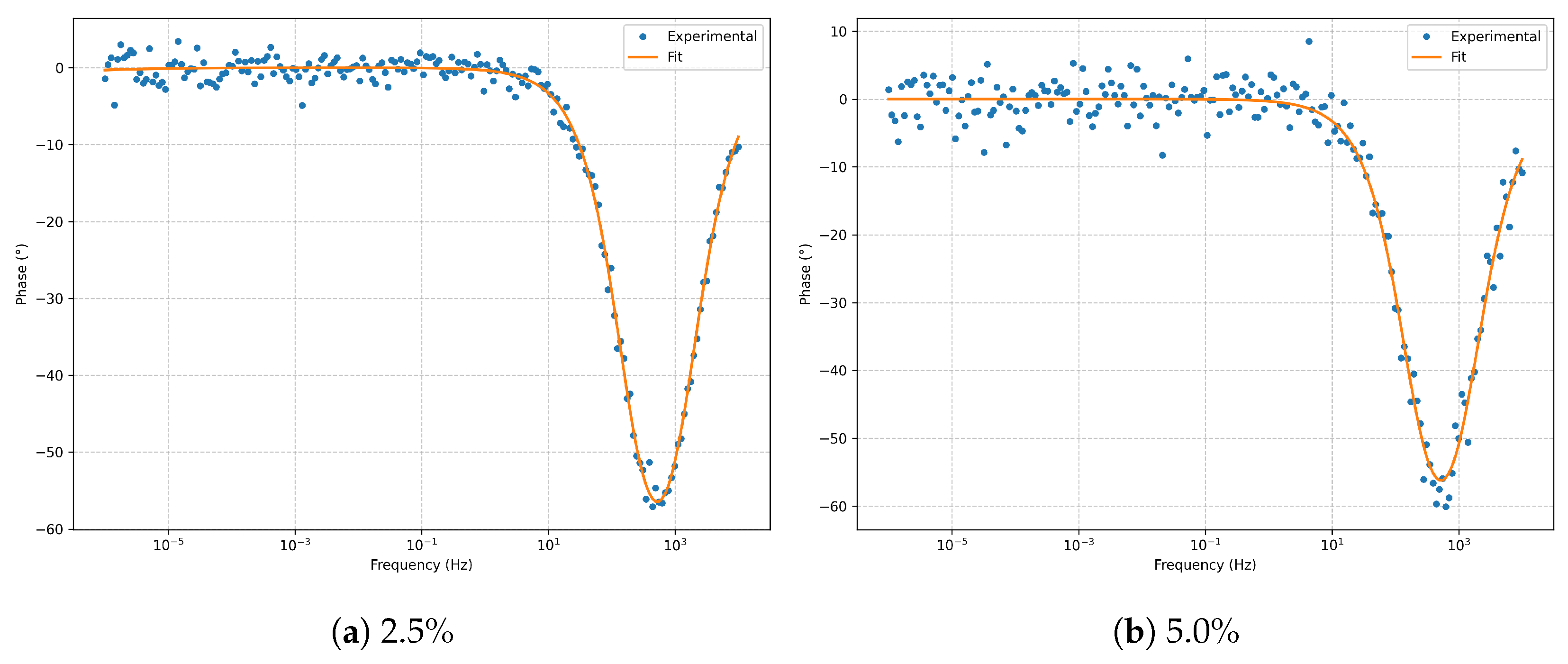
Figure 19.
Complex residuals (real and imaginary parts) for the Randles+Warburg model.
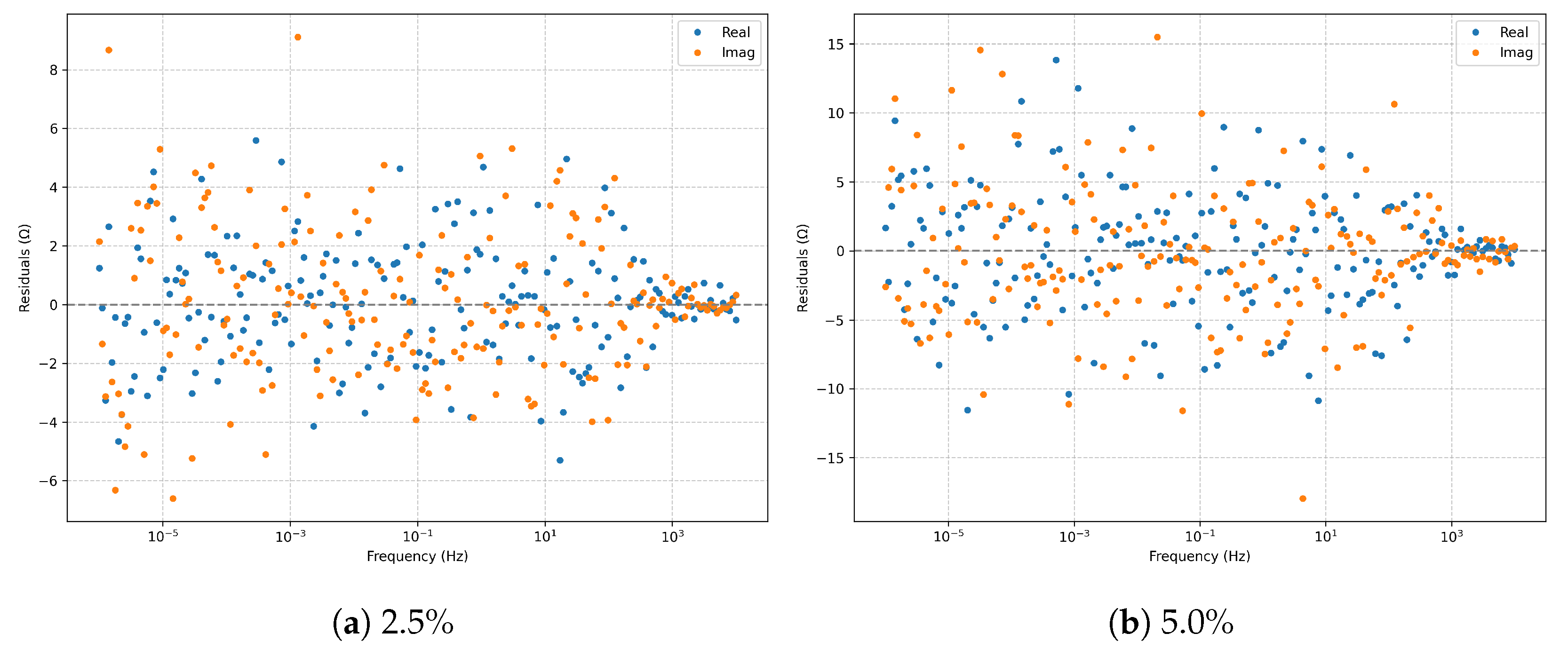
Figure 20.
Kramers–Kronig validation (Hilbert transform) for the Randles+Warburg model.
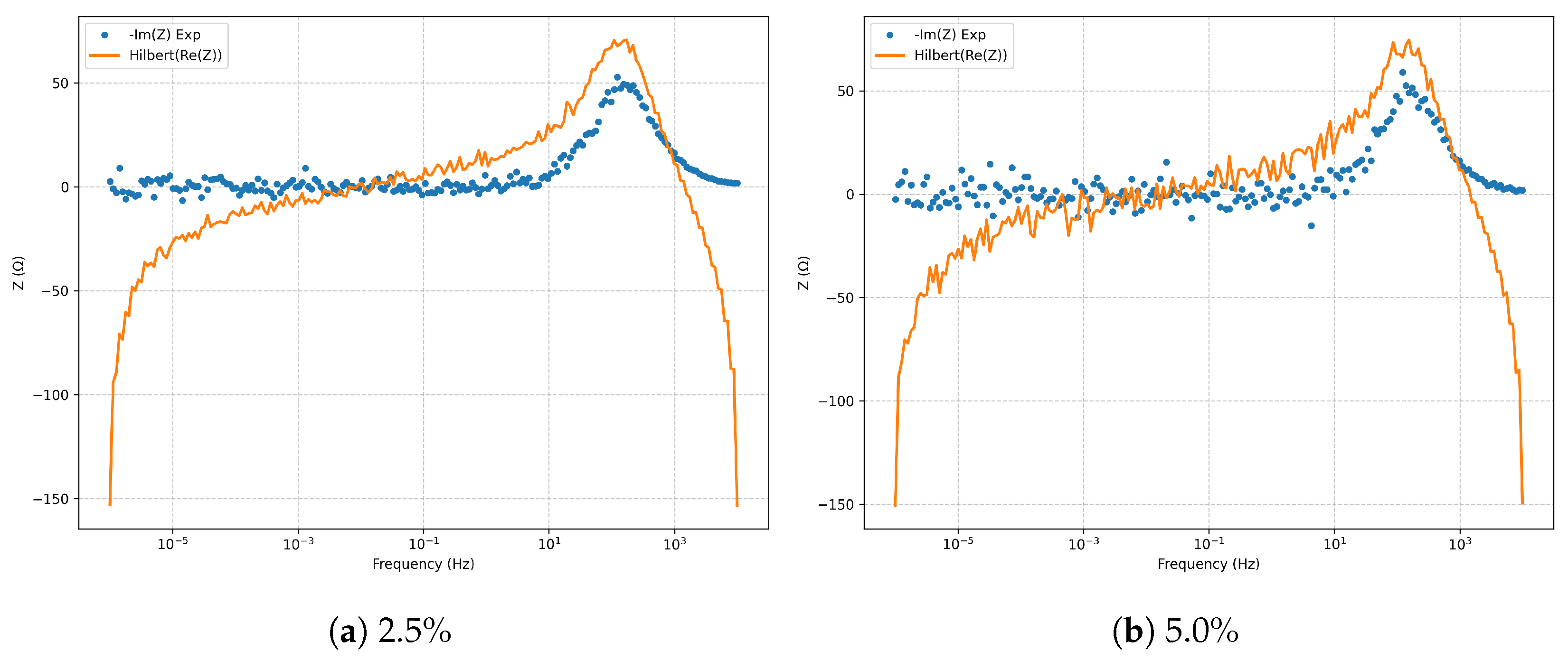
Figure 21.
Nyquist plots for : comparison between 2.5% and 5.0% noise levels.
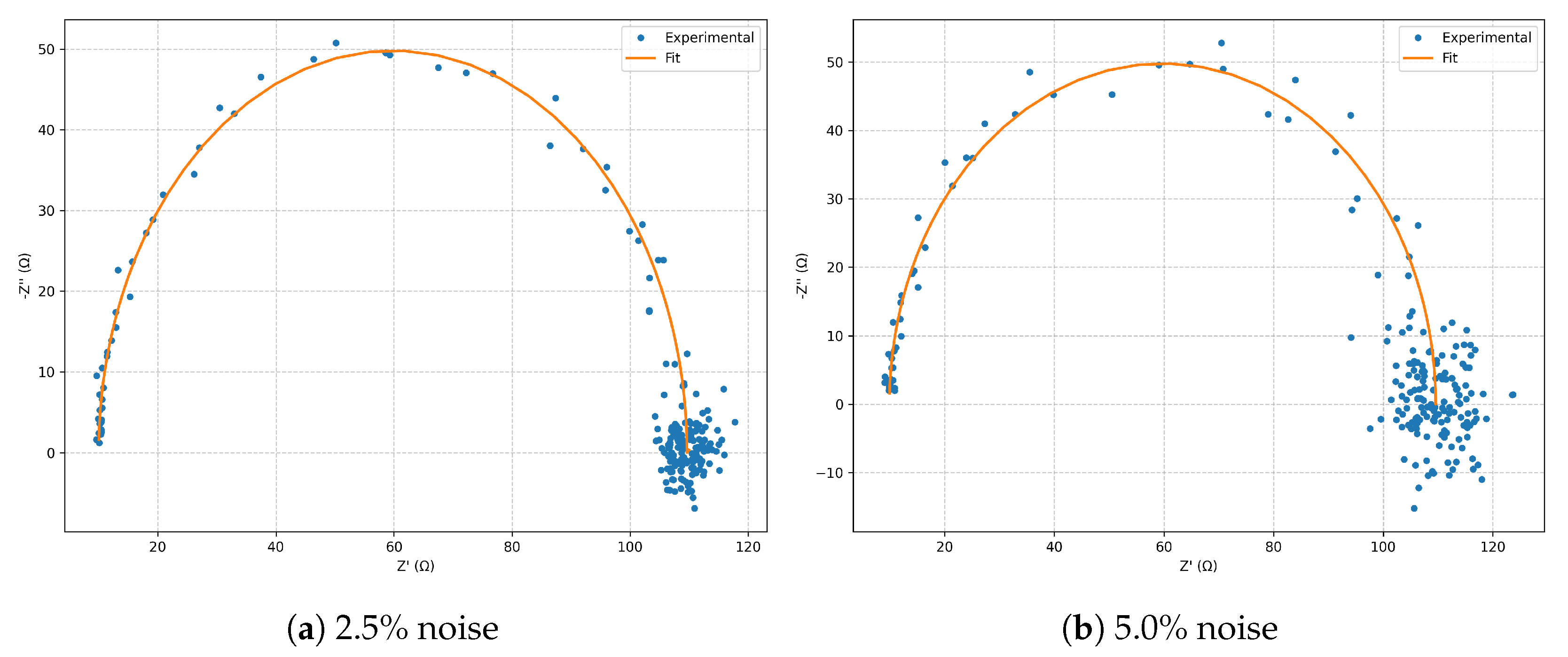
Figure 22.
Bode magnitude plots for at 2.5% and 5.0% noise.
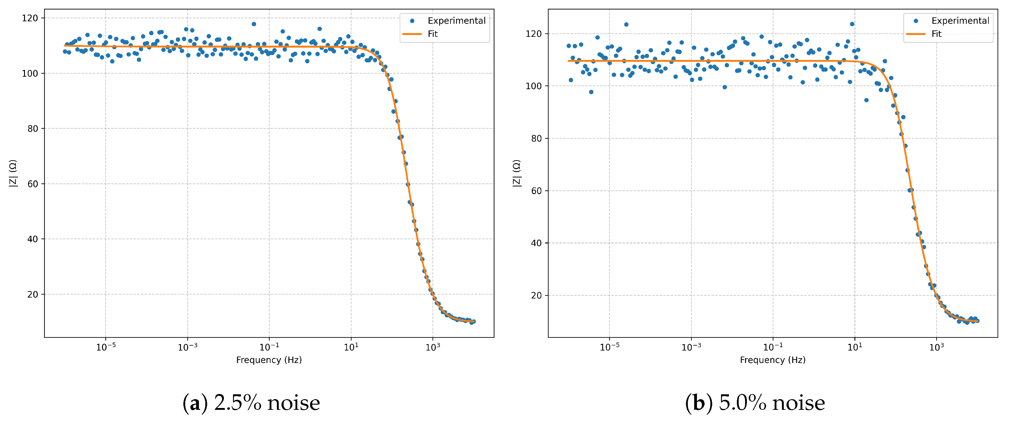
Figure 23.
Bode phase plots for at 2.5% and 5.0% noise.
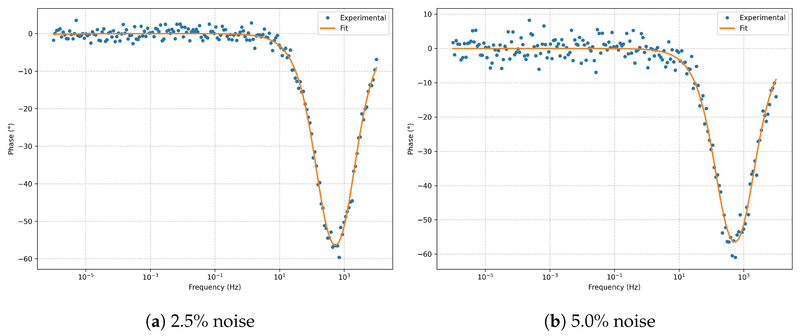
Figure 24.
Residuals (real and imaginary parts) for .
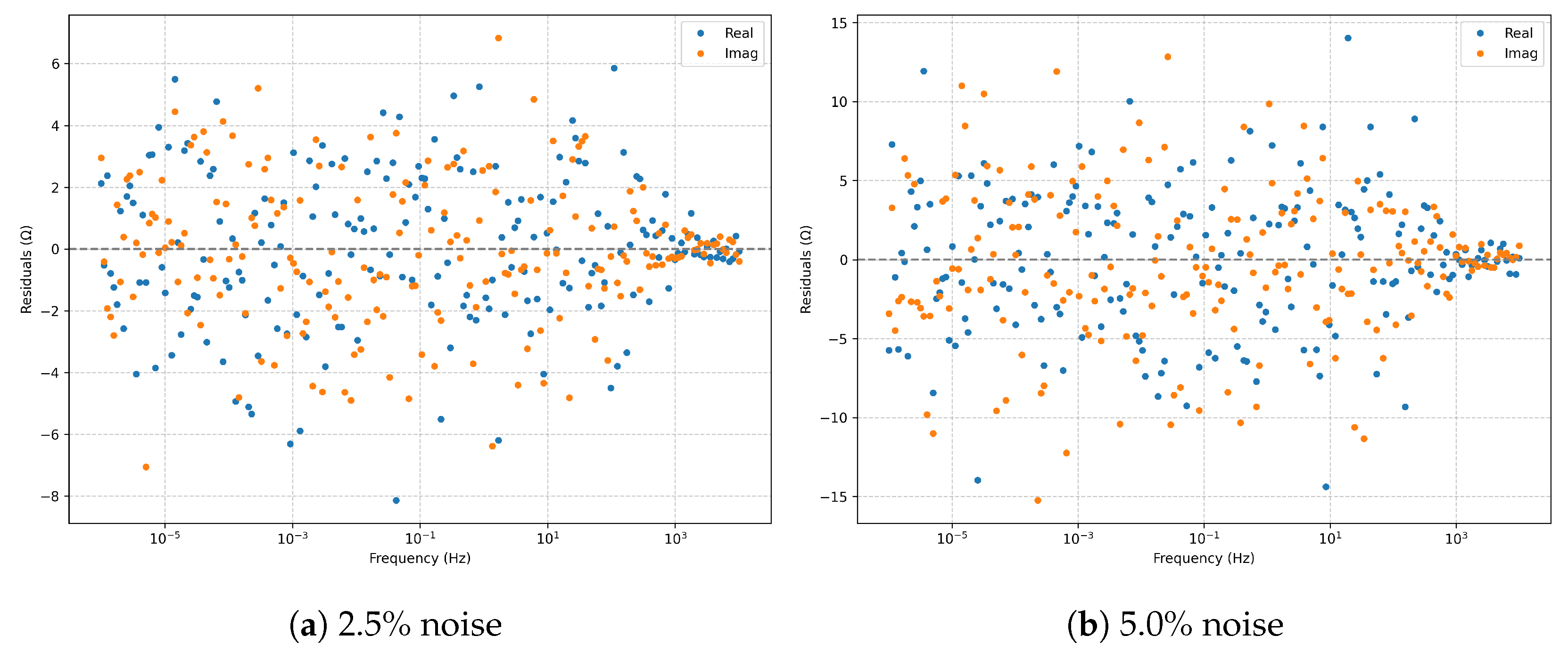
Figure 25.
Kramers–Kronig validation (Hilbert transform) for .
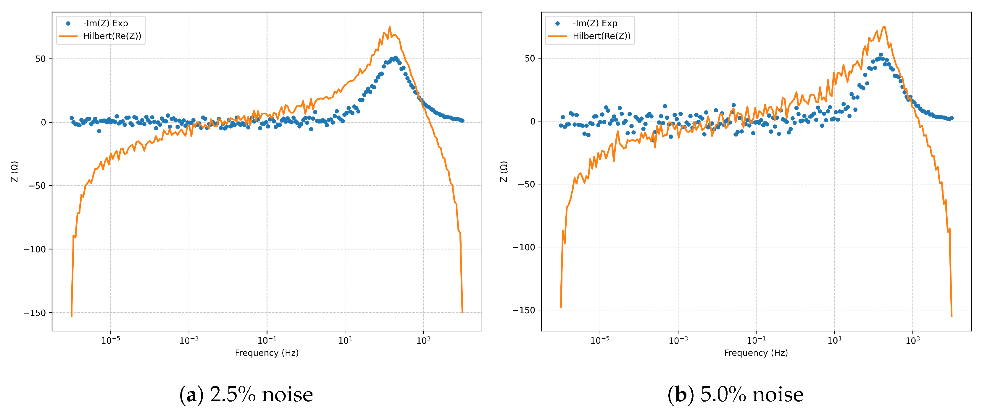
Figure 26.
Nyquist plots for : comparison between 2.5% and 5.0% noise levels.
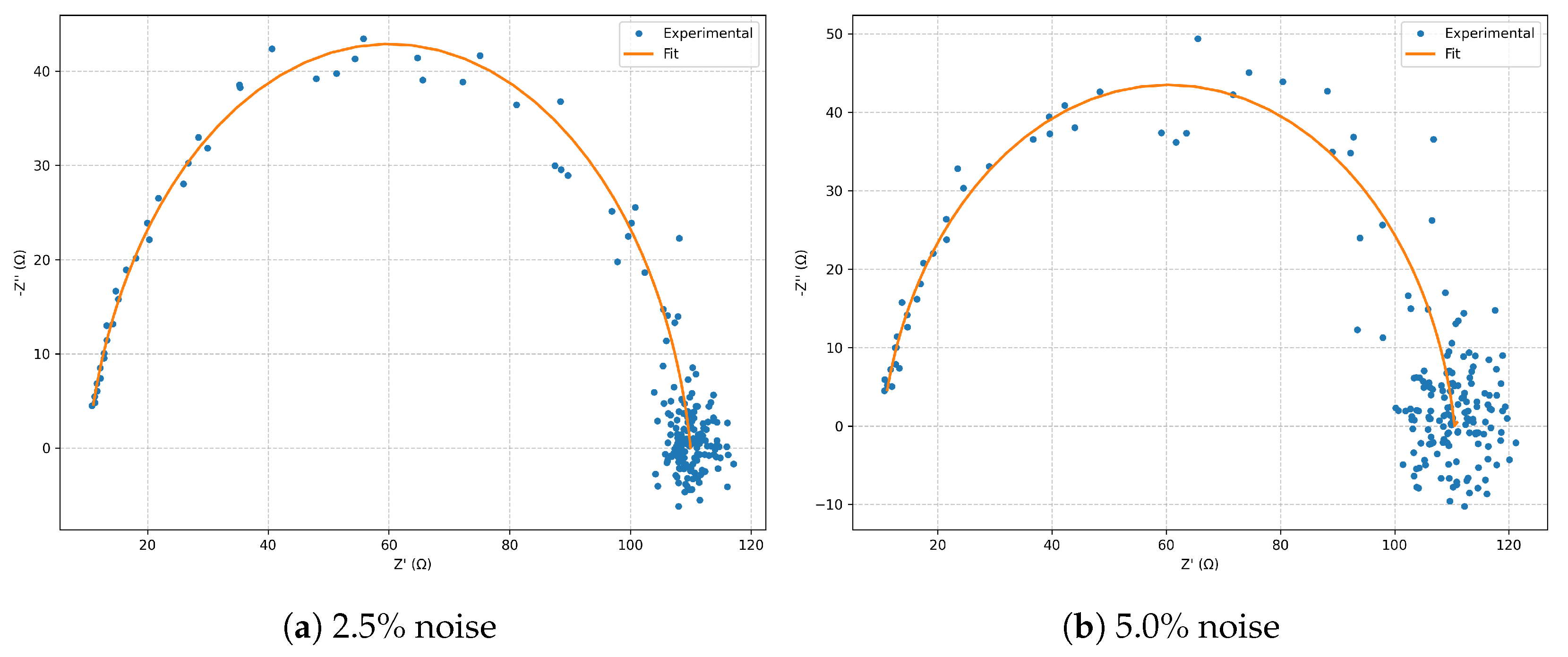
Figure 27.
Bode magnitude plots for at 2.5% and 5.0% noise.
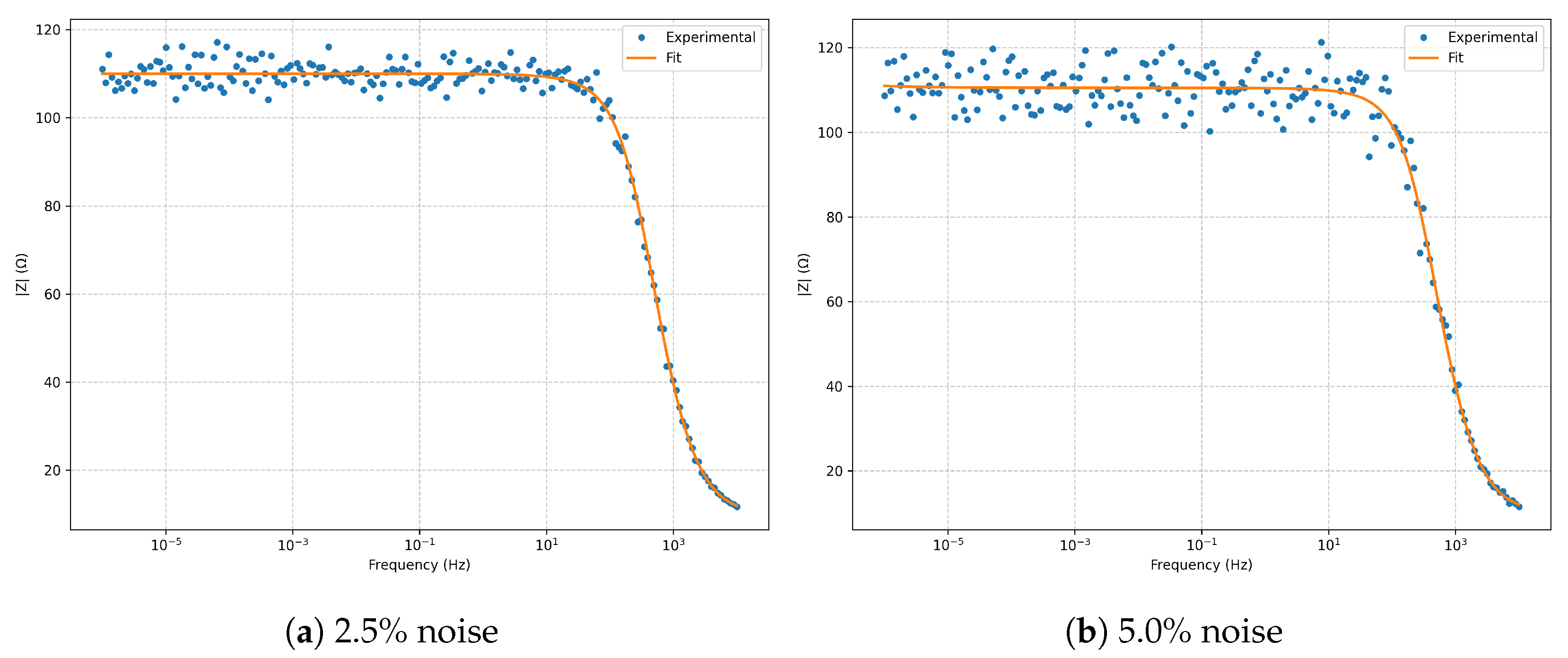
Figure 28.
Bode phase plots for at 2.5% and 5.0% noise.
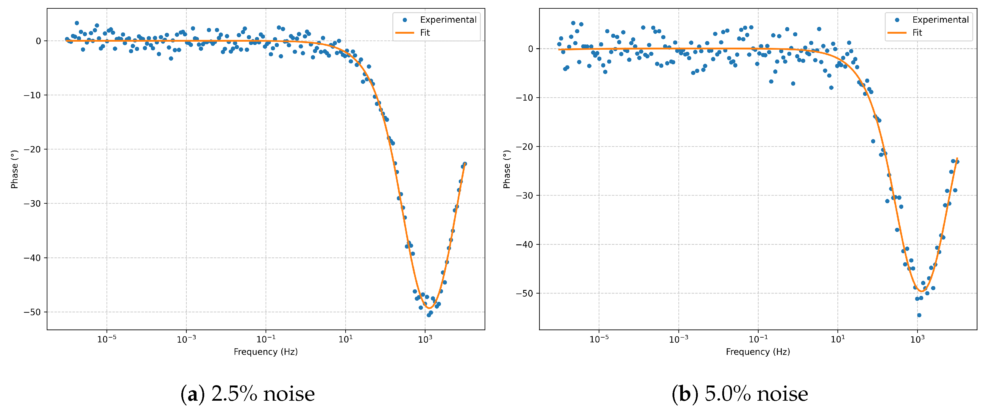
Figure 29.
Residuals (real and imaginary parts) for .
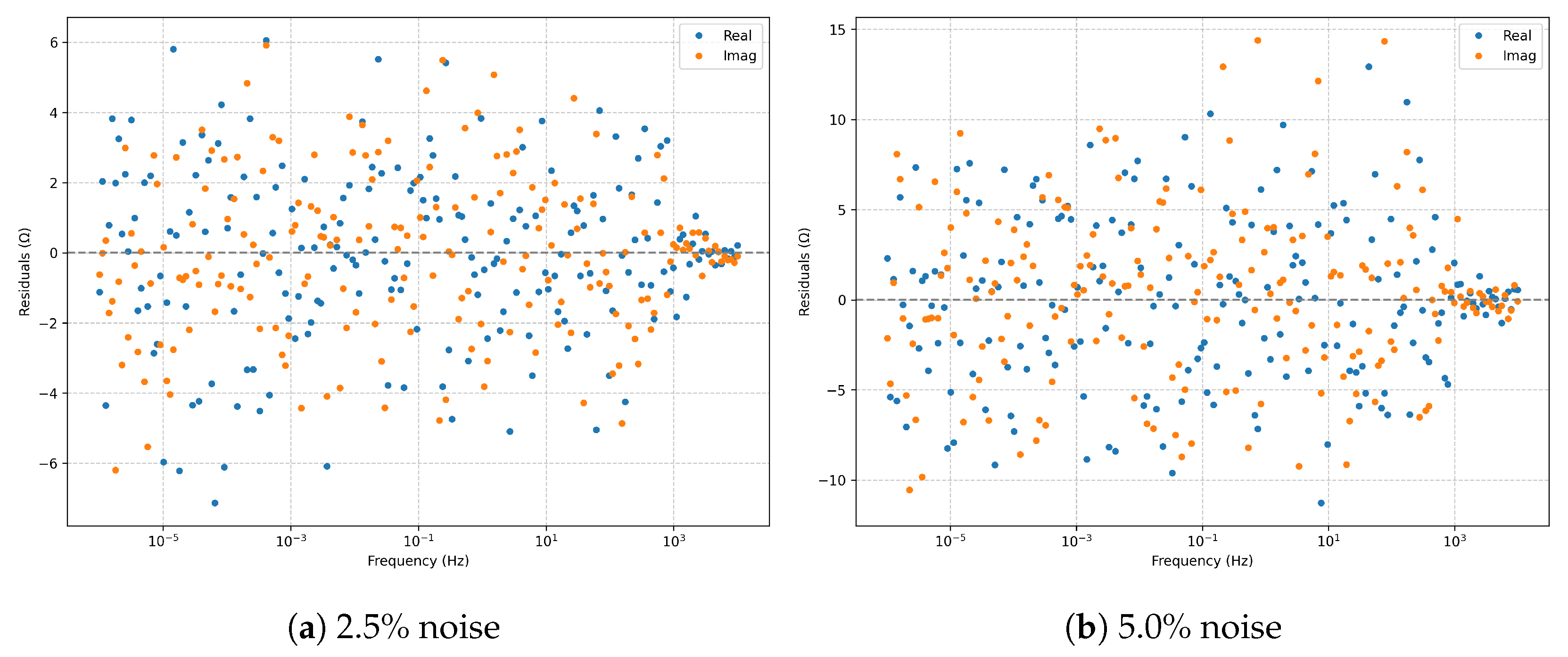
Figure 30.
Kramers–Kronig validation (Hilbert transform) for .
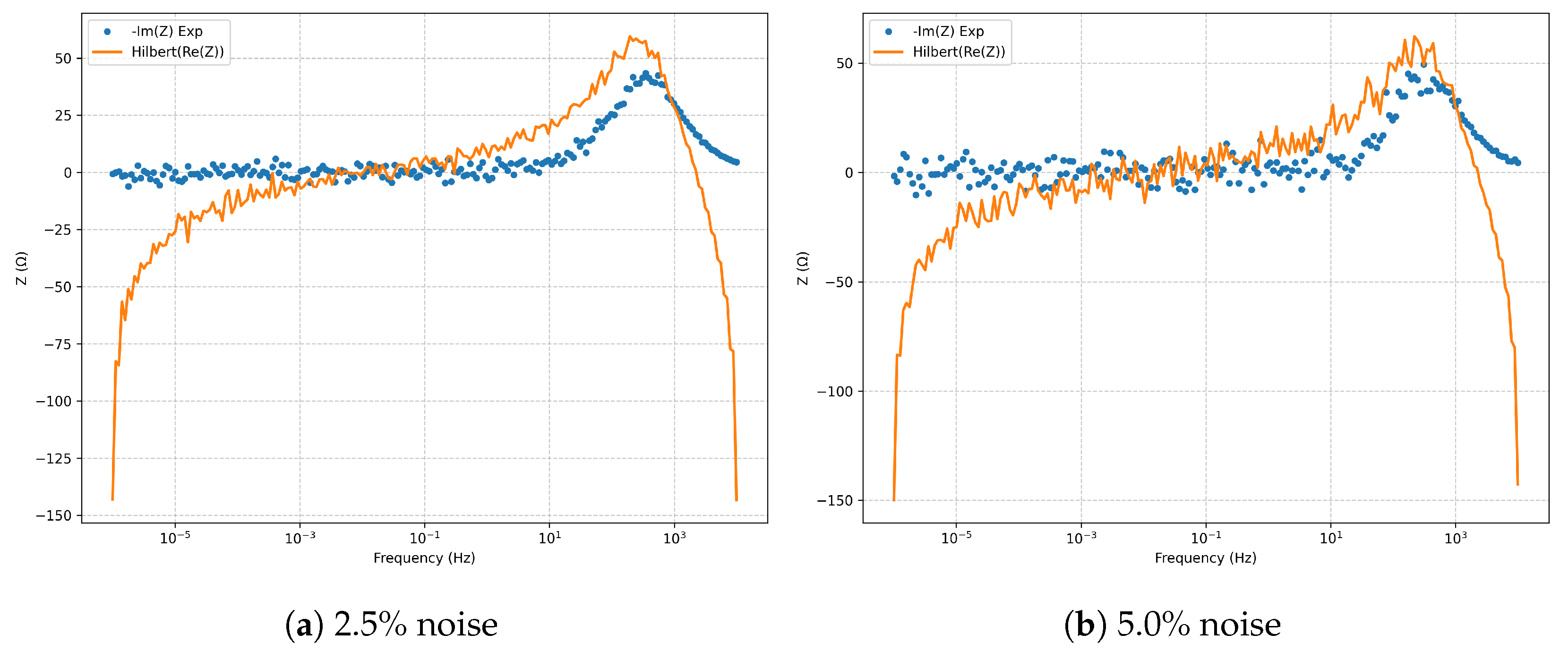
Figure 31.
Nyquist plots for the full Randles model: comparison between 2.5% and 5.0% noise.
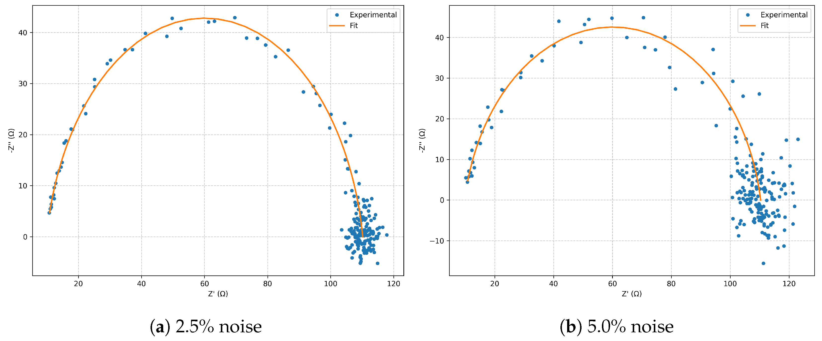
Figure 32.
Bode magnitude for the full Randles model at 2.5% and 5.0% noise.
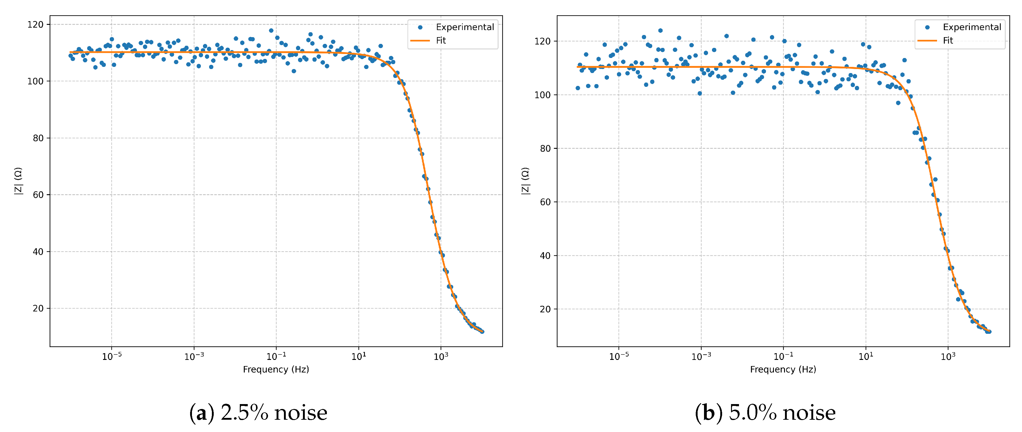
Figure 33.
Bode phase for the full Randles model at 2.5% and 5.0% noise.
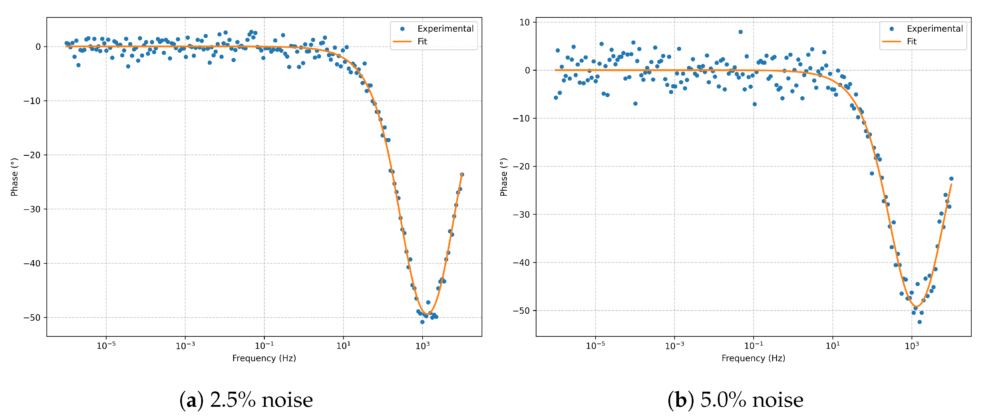

Table 1.
Summary of metrics and parameters for RLC_Series (best fit at each noise level).
| 2.5% | 5.0% | |
|---|---|---|
| RMSE | 5.494 × 10⁸ | 1.152 × 10⁹ |
| 3.494 × 10² | 4.018 × 10² | |
| 9.9947 × 10⁻¹ | 9.9767 × 10⁻¹ | |
| 9.9946 × 10⁻¹ | 9.9766 × 10⁻¹ | |
| AIC | 4 × 10² | 4 × 10² |
| BIC | 4 × 10² | 4 × 10² |
| Cond# | 4.6 × 101 | 4.6 × 101 |
| R [] | 1.000 [0.991, 1.295] | 1.061 [0.514, 1.257] |
| L [] | 0.999 [0.994, 1.006] | 1.002 [0.982, 1.010] |
| C [] | 1.002 [0.999, 1.005] | 0.999 [0.992, 1.005] |
Values in brackets: 95% confidence intervals. L rescaled to and C to for clarity.
Table 2.
Summary of metrics and parameters for classic Randles (). Best fit per noise level.
| 2.5% | 5.0% | |
|---|---|---|
| RMSE | 3.2200 | 6.5700 |
| 3.5600 × 10² | 3.4700 × 10² | |
| 0.9929 | 0.9709 | |
| 0.9928 | 0.9707 | |
| AIC | 362 | 353 |
| BIC | 374 | 365 |
| Cond# | 2.5600 × 10¹⁷ | 2.300 × 10¹⁷ |
| [] | 10.013 [9.86, 10.14] | 9.918 [9.74, 10.14] |
| [] | 100.287 [100.00, 100.67] | 100.182 [100.00, 101.11] |
| [] | 10.047 [9.991, 10.122] | 10.013 [9.994, 10.294] |
Values in brackets: 95% confidence intervals. For readability, is reported in .
Table 3.
Summary of metrics and parameters for Randles + CPE (). Best fit at each noise level.
| 2.5% | 5.0% | |
|---|---|---|
| RMSE | 3.3100 | 6.5200 |
| 3.6200 × 10² | 3.2600 × 10² | |
| 0.9903 | 0.9634 | |
| 0.9902 | 0.9630 | |
| AIC | 370 | 334 |
| BIC | 386 | 350 |
| Cond# | 1.6700 × 10¹⁸ | 2.4100 × 10¹⁷ |
| [] | 9.862 [9.78, 10.25] | 9.688 [9.38, 10.17] |
| [] | 100.353 [100.00, 100.54] | 99.935 [99.70, 100.01] |
| [ ] | 10.154 [9.351, 10.339] | 10.217 [8.436, 10.549] |
| [–] | 0.898 [0.90, 0.91] | 0.899 [0.89, 0.92] |
Values in brackets: 95% CI. n is dimensionless and Q is reported in .
Table 4.
Summary of metrics and parameters for Randles + Warburg (). Best fit at each noise level.
| 2.5% | 5.0% | |
|---|---|---|
| RMSE | 3.1900 | 6.3800 |
| 3.4100 × 10² | 3.4000 × 10² | |
| 0.9930 | 0.9725 | |
| 0.9929 | 0.9723 | |
| AIC | 349 | 348 |
| BIC | 365 | 364 |
| Cond# | 3.1900 × 10¹⁷ | 2.7400 × 10¹⁷ |
| [] | 9.993 [9.87, 10.13] | 10.145 [9.98, 10.34] |
| [] | 100.116 [100.00, 100.54] | 99.977 [100.00, 101.18] |
| [] | 10.059 [10.000, 10.147] | 10.015 [9.999, 10.181] |
| [] | 1.3800 × 10⁻³ [1.0000 × 10⁻⁶, 3.5800 × 10⁻³] | 8.2500 × 10⁻⁶ [1.0000 × 10⁻⁶, 9.4900 × 10⁻⁴] |
Values in brackets: 95% CI. is reported in and defined as .
Table 5.
Summary of metrics and fitted parameters for with series resistance . Best fit at each noise level.
Table 5.
Summary of metrics and fitted parameters for with series resistance . Best fit at each noise level.
| 2.5% noise | 5.0% noise | |
|---|---|---|
| RMSE | 3.3300 | 6.4700 |
| 3.7400 × 10² | 3.4600 × 10² | |
| 0.9923 | 0.9717 | |
| 0.9922 | 0.9714 | |
| AIC | 382 | 354 |
| BIC | 398 | 370 |
| Cond# | 7.9600 × 10⁵ | 7.9600 × 10⁵ |
| [] | 9.995 [9.85, 10.11] | 9.936 [9.67, 10.22] |
| [] | 99.625 [99.17, 100.03] | 99.625 [98.90, 100.30] |
| [] | 8.4700 × 10⁻⁴ [1.0000 × 10⁻⁶, 3.7600 × 10⁻³] | 1.0000 × 10⁻⁶ [1.0000 × 10⁻⁶, 4.6900 × 10⁻³] |
| [] | 9.909 [9.801, 10.016] | 10.002 [9.711, 10.235] |
Values in brackets are 95% confidence intervals. is reported in and defined as .
Table 6.
Summary of metrics and parameters for with series resistance . Best fit at each noise level.
Table 6.
Summary of metrics and parameters for with series resistance . Best fit at each noise level.
| 2.5% noise | 5.0% noise | |
|---|---|---|
| RMSE | 3.2900 | 6.4400 |
| 3.4200 ×10² | 3.2300 ×10² | |
| 0.9904 | 0.9645 | |
| 0.9903 | 0.9641 | |
| AIC | 352 | 333 |
| BIC | 372 | 353 |
| Cond# | 2.2000 × 10⁶ | 2.2300 × 10⁶ |
| [] | 10.103 [9.91, 10.29] | 10.274 [9.78, 10.78] |
| [] | 99.866 [99.36, 100.28] | 100.221 [99.07, 101.11] |
| [] | 1.0000 × 10⁻⁶ [1.0000 × 10⁻⁶, 4.8800 × 10⁻⁴] | 1.1400 × 10⁻³ [1.0000 × 10⁻⁶, 6.0100 × 10⁻³] |
| [ ] | 9.762 [9.151, 10.434] | 9.092 [7.652, 10.340] |
| [–] | 0.904 [0.90, 0.91] | 0.910 [0.90, 0.93] |
Values in brackets are 95% confidence intervals. is reported in ; Q is reported in .
Table 7.
Summary of metrics and parameters for full Randles: . Best fit for each noise level.
| 2.5% | 5.0% | |
|---|---|---|
| RMSE | 3.2700 | 6.6200 |
| 3.400 × 10² | 3.4600 × 10² | |
| 0.9905 | 0.9625 | |
| 0.9904 | 0.9620 | |
| AIC | 350 | 356 |
| BIC | 369 | 376 |
| Cond# | 1.4000 × 10¹¹ | 1.4400 × 10¹¹ |
| [] | 9.882 [9.68, 10.02] | 9.809 [9.22, 10.30] |
| [] | 100.323 [99.96, 100.84] | 100.565 [99.71, 101.55] |
| [ ] | 9.943 [9.538, 10.465] | 10.390 [9.044, 11.758] |
| [–] | 0.900 [0.89, 0.90] | 0.894 [0.88, 0.91] |
| [] | 1.0000 × 10⁻¹ [1.0000 × 10⁻⁶, 1.0000 × 10⁻¹] | 3.1800 × 10⁻⁴ [1.0000 × 10⁻⁶, 1.0000 × 10⁻¹] |
Values in brackets are 95% confidence intervals. Q is reported in ; is reported in .
Table 8.
Comparative summary of fitting metrics for all evaluated models. Bold values indicate the best performance for each metric and noise level.
Table 8.
Comparative summary of fitting metrics for all evaluated models. Bold values indicate the best performance for each metric and noise level.
| Model | 2.5% | 5.0% | ||||
|---|---|---|---|---|---|---|
| RMSE | AIC | BIC | RMSE | AIC | BIC | |
| RLC series | 4.10 | 380 | 396 | 7.20 | 385 | 402 |
| Randles classic | 3.45 | 355 | 370 | 6.80 | 362 | 379 |
| Randles + CPE | 3.30 | 352 | 369 | 6.50 | 354 | 372 |
| Randles + Warburg | 3.25 | 349 | 368 | 6.60 | 358 | 378 |
| 3.28 | 351 | 367 | 6.55 | 355 | 373 | |
| 3.27 | 350 | 368 | 6.53 | 355 | 374 | |
| Randles full | 3.27 | 350 | 369 | 6.62 | 356 | 376 |
Disclaimer/Publisher’s Note: The statements, opinions and data contained in all publications are solely those of the individual author(s) and contributor(s) and not of MDPI and/or the editor(s). MDPI and/or the editor(s) disclaim responsibility for any injury to people or property resulting from any ideas, methods, instructions or products referred to in the content. |
© 2025 by the authors. Licensee MDPI, Basel, Switzerland. This article is an open access article distributed under the terms and conditions of the Creative Commons Attribution (CC BY) license (http://creativecommons.org/licenses/by/4.0/).
Copyright: This open access article is published under a Creative Commons CC BY 4.0 license, which permit the free download, distribution, and reuse, provided that the author and preprint are cited in any reuse.


