
Submitted:
17 September 2025
Posted:
25 September 2025
You are already at the latest version
Abstract
Electrochemical impedance spectroscopy (EIS) is a widely used technique for analyzing battery dynamics over a broad frequency spectrum. Conventional state-of-the-art EIS methods involve applying a sequence of sinusoidal excitation signals, ranging from very low to very high frequencies, to capture the impedance response of the battery. However, this process is time-consuming, often requiring several hours to complete. Alternatively, approaches using pulse-based excitation have shown promise in reducing test time but often suffer from challenges in handling measurement noise and poor frequency resolution, especially at low frequencies. This work presents an improved rectangular pulse-based impedance characterization technique that enhances low-frequency resolution, increases robustness to noise, and reduces experimental time. This is accomplished through the following three key contributions of this paper: First, it establishes statistical noise properties in the Fourier-transformed signals, enabling effective noise reduction through averaging. Second, it proposes a log-frequency clustering approach to average impedance data, enhancing the accuracy of the impedance spectrum. Third, it presents a systematic pulse design method using the knowledge of the approximate time constants of the system to select the sampling interval, pulse width, and rest duration for reduced test time, improved low-frequency resolution, and enhanced signal-to-noise ratio (SNR). Together, the proposed approach enables faster, and a more accurate impedance characterization. Simulation analysis and experimental results confirm that the proposed approach enhances spectral resolution at low frequencies, mitigates the impact of noise at high frequencies, and significantly improves the reliability of impedance estimates at a faster measurement time-frame.
Keywords:
battery management systems
; electrochemical impedance spectroscopy
; battery testing
; impedance analysis
; state of health
1. Introduction
Electrochemical impedance spectroscopy (EIS) is a well-established method for analyzing the dynamic behavior of electrochemical systems, including batteries, [1,2,3]. The impedance parameters derived from the EIS play a central role in estimating the key battery states such as state of charge (SOC) [4,5], state of health (SOH) [6,7,8,9,10], and remaining useful life (RUL) [11]. Leveraging the EIS within battery management systems (BMS) enables accurate battery state estimation that improves the performance, safety, and reliability in applications, such as electric vehicles (EVs) and energy storage systems.
1.1. Literature Review
State-of-the-art EIS techniques involve applying small amplitude sinusoidal current signals at multiple discrete frequencies, typically spanning from low to high, and measuring the resulting voltage to construct the impedance spectrum [12,13,14]. While effective, this approach is inherently time-consuming, especially at low frequencies, which limits its practical utility in real-time applications. To address this limitation, pulse-based excitation methods have gained attention due to their ability to significantly shorten the measurement time while still enabling accurate impedance estimation [15,16,17,18,19,20,21,22]. Unlike sinusoidal excitation, which captures information at a single frequency and requires sequential sweeps, pulse excitation excites a broad range of frequency components at once, making it a more efficient alternative. By applying a fast Fourier transform (FFT) [23] to the input current and the concomitant voltage response, the impedance spectrum can be derived, enabling analysis in the frequency domain.
In [24], a voltage step signal was utilized as the excitation source for impedance analysis, while the authors in [25] employed both step and pulse current signals to estimate the impedance. In both studies, the impedance spectrum was derived by applying the Laplace transform to the input and output signals. A novel method was proposed in [26] to extract the impedance spectrum directly from the pulse charge/discharge curves of batteries, offering an alternative approach to traditional EIS techniques. In [27], a rapid computation method for broadband battery impedance utilizing the S-transform employing Gaussian window was introduced. Furthermore, wavelet transform-based methods were explored in [28,29,30], where pulse current and voltage signals were analyzed in the time-frequency domain to extract the impedance information, highlighting the potential of wavelet analysis for EIS. In a broader comparison, authors in [31] investigated various excitation signals, including rectangular pulses, Gaussian inputs, and sinc waveforms, and compared their resulting impedance spectra against those obtained through standard sinusoidal excitation.
1.2. Research Gap & Motivation
Although pulse-based methods have demonstrated strong potential as faster and more efficient alternatives to conventional EIS, several critical challenges remain unaddressed in the literature. A primary limitation lies in the sensitivity to noise, particularly in the high-frequency region where the signal-to-noise ratio (SNR) tends to degrade. This often results in unreliable impedance estimates when compared with sinusoidal excitation. While studies such as [12,13] have systematically analyzed noise effects in sinusoidal-based EIS, equivalent investigations for pulse-based approaches are sparse. As a result, the robustness of pulse excitation under realistic measurement conditions remains insufficiently understood.
Another important gap concerns the systematic selection of pulse design parameters, including sampling frequency, pulse duration, and relaxation period, which directly determine the spectral content and resolution of the resulting impedance. Existing works on step or pulse excitations [24,25,26] demonstrate feasibility but provide little methodological guidance on parameter tuning for accurate and reliable impedance estimation across the full frequency range. In particular, the low-frequency region suffers from limited resolution, and improper choice of excitation parameters can further compromise accuracy.
Moreover, while alternative signal processing methods such as wavelet transforms [28,29,30] and generalized excitation signal comparisons [31] have been explored, there is still no unified framework linking pulse signal design, noise robustness, and impedance estimation accuracy.
By systematically analyzing the interplay of noise, excitation parameters, and spectral resolution, this work aims to establish clear methodological guidelines for pulse-based impedance estimation, thereby enabling faster, more robust, and accurate characterization of batteries in real-world settings.
1.3. Contributions
The key contributions of this paper are outlined below
- Statistical analysis of the noise characteristics: The first major contribution of this work is the analytical derivation of the statistical property, i.e., the mean of the Fourier-transformed voltage noise, current noise, and resulting impedance noise. This paper mathematically shows that the voltage and current measurement noises retain their zero-mean property in the frequency domain. This property enables effective noise reduction in the raw impedance estimates through averaging, leading to a significant improvement in the accuracy of the impedance spectrum.
- Zero-padding approach to improve resolution: The impedance spectrum derived from the proposed rectangular pulse excitation exhibits a non-uniform distribution of impedance estimates across the frequency range. There is a higher concentration of estimates in the high-frequency region and fewer in the low-frequency region. To enhance the resolution in the low-frequency domain, a zero-padding technique is introduced.
- Log-scaled frequency clustering for improved spectral representation: To address the imbalance in the number of measurements across different frequencies, a log-scale clustering strategy is proposed. By grouping impedance values into logarithmically spaced frequency bins and averaging within each bin, a more uniform and noise-reduced spectral representation is obtained across the frequency ranges.
- Time-constant informed rectangular pulse design for accurate characterization: This paper also introduces a systematic method for designing rectangular pulse excitation signals, based on the knowledge of the approximate time constants of the system. It offers practical recommendations for selecting the sampling interval, pulse width, and zero-current duration, with the goal of reducing the experimental time, enhancing low-frequency spectral resolution, and improving the SNR.
1.4. Organization of the Paper
The remainder of this paper is organized in the following sections : Section 2 introduces the rectangular pulse excitation signal and its transformation in the frequency domain using Fourier transform. Statistical analysis of the impedance noise is performed in Section 3. Section 4 discusses the design of the excitation signal for improved SNR. Simulation analyses are provided in Section 5, whereas the experimental procedures and results are detailed in Section 6. The paper is concluded in Section 7.
2. Rectangular Pulse Excitation Signal
This section discusses the characterization of the electrochemical impedance behaviour of Li-ion batteries using a rectangular pulse excitation signal. Figure 1 shows a rectangular excitation current signal (in blue) and typical battery response (in red).
The equivalent circuit model (ECM) of the battery is shown in Figure 2, which consists of (i) a voltage source in open-circuit condition, , (ii) ohmic resistance, , and (iii) two RC circuits with RC-pairs , and and (iv) Warburg impedance at very low frequencies.
The voltage response, of the battery corresponding to the input , is depicted in red in Figure 1.
The impedance response, , for a given frequency, , is determined as
where and are the frequency transforms of , and respectively, obtained by Fourier transform. For further details on battery modeling and EIS theory, refer to [32]. Figure 3 shows the typical impedance response of a battery.
The rectangular pulse excitation signal shown in Figure 1 can be discretized by sampling at intervals of `’ seconds. Let `K’ denote the number of samples in the `ON’ duration of the pulse, i.e., , and the total number of samples in the signal be denoted as . The discrete rectangular pulse signal, , shown in Figure 4, is defined as
For DFT, the continuous frequency `’ of the transform is discretised to `N’ frequency bins as
where is the sampling frequency, and is the frequency resolution of the transform, which denotes the spacing between frequency bins in the DFT.
The DFT of the current signal, , which is a vector of values, is given by,
Refer to Appendix A for the details of this transformation, which can be written as , for , and
The DFT of the response, , is given by,
3. Mean and Variance of the Impedance Noise
This section presents a statistical analysis of impedance noise.
3.1. Mean of the Impedance Noise
Let us denote the measured voltage from the battery in vector format as
where is the true voltage signal and is the voltage noise vector.
The DFT of the measured voltage, , can be written as
where is the unitary DFT matrix given by
and, and are given by
Similarly, the DFT of the input current can be written as
where and are given by
See Appendix B for details on how the zero-mean property of voltage and current noise is preserved in the frequency domain.
Let us now consider the impedance at the frequency bin
where is the row of which is denoted for simplicity as
By recognizing that , let us decompose it into its real and complex parts as
Now, can be written as
where and are the real and imaginary parts, respectively, of the impedance. This can be further written according to the signal and noise portions as follows
where
and , are given below.

It can be verified that
4. Excitation Signal Design for Improved SNR
4.1. Selection of Sampling Time,
The sampling time should be chosen to accurately capture the system dynamics associated with the smallest time constant [33]. As a rule of thumb, it should be less than one-tenth of the system’s minimum time constant, i.e.,
where for the ECM shown in Figure 2, the system’s minimum time constant is determined by the smallest RC product, i.e.,
Remark 1.
There is a trade-off in selecting the sampling time .
- 1
- Smaller : The advantage of smaller is that, the high-frequency response of the battery is accurately captured. However, choosing a very small can be challenging to implement in practice.
- 2
- Larger : Larger reduces the volume of collected data, lowering the computational load. However, it limits the ability to capture high-frequency impedance features and introduces the risk of aliasing if fast dynamics are present.
4.2. Selection of
This section discusses how the minimum for the pulse design is determined based on the zero-crossings in the frequency spectrum. The DFT of the current excitation signal is given in (A2). To determine the points `m’ where this signal crosses zero, i.e., to find the zero-crossings, we set
which is
The zero-crossings occur when,
This means that,
where p is an integer. Then,
where is the duty-cycle of the pulse. This implies that the zero-crossings of the excitation signal’s spectrum occur at integer multiples of , or equivalently, at integer multiples of . The total number of zero-crossings, , within frequency bins – equivalent to – is
The lowest corresponds to a rectangular pulse whose total number of zero-crossings, , is minimized. In this design, the main lobe of the spectrum will exclusively span all frequencies of interest up to the system’s maximum frequency, corresponding to . This requires that the first and only zero-crossing of the spectrum occurs at
In terms of frequency, (32) translates to , which crosses zero at , i.e.,
Solving this yields,
Based on the criteria for sampling time in (24), the criteria for minimum in (34) can be written as,
Thus, for the pulse design can be chosen as
Remark 2.
There is a trade-off in selecting the pulse duration .
- 1
- Smaller : The advantage of smaller is that it reduces the number of zero-crossings in the excitation spectrum. Smaller ensures that the amplitudes of the main and side lobes remain relatively close, which means that the excitation amplitude stays nearly constant across all frequencies. Another advantage of smaller is that it reduces the total experiment time. Finally, smaller reduces the effect to the OCV during the experiment thereby ensuring that the battery’s operating condition is not significantly altered during the experiment.
- 2
- Larger : Larger leads to a significantly larger main lobe amplitude in the excitation spectrum. Since zero-crossings occur at integer multiples of , a higher duty cycle results in a narrower main lobe, concentrating more energy at low frequencies. This characteristic is particularly advantageous for accurately estimating the low-frequency resistance of the battery.
4.3. Selection of
With set, the zero-current duration of the excitation signal, , can be chosen to be atleast ten times the system’s largest time constant, i.e.,
which provides sufficient time for the dynamics of the system to settle. The total duration of the excitation signal, is given by
where and are determined based on the system’s time constants.
4.4. Zero-Padding
In [34], was chosen to achieve a desired frequency resolution for the DFT. In this paper, its selection is refined based on the knowledge of the system’s time constants. To further improve low-frequency resolution, zero-padding is applied by appending zeros to the time-domain signal prior to the DFT, increasing the number of frequency bins and reducing their spacing. This enhances low-frequency detail in the impedance spectrum without increasing the actual experiment duration.
5. Simulation Analysis
This section presents the analysis of pulse-based EIS through simulations conducted in MATLAB. In this paper, it is assumed that to eliminate any bias effects caused by the OCV. The following parameters of the ECM are used in the simulations : , , , , , and diffusion effects are assumed to be zero. The impedance, , for the ECM depicted in Figure 2 is theoretically expressed as
Figure 5(a) shows the theoretical impedance spectrum i.e., the magnitude of impedance versus frequency for a range of frequencies between 0 Hz and 1000 Hz. When the frequency is zero, the impedance of the circuit is the sum of resistances, . Theoretically, at infinite frequency, the impedance of the circuit is its ohmic resistance, .
The section of the plot in Figure 5(b) between markers and ∇ indicates the low frequency impedance response. It can be determined from Figure 5(a) that, the corresponding low frequency range varies between 0 Hz and ≈ 0.6 Hz. The section of the plot in Figure 5(b) between ∇ and + is the high frequency response of the circuit, with frequencies ranging from 0.6 Hz to 500 Hz.
The following demonstrations illustrate the effects of varying and , applying zero-padding, and changing the SNR levels on the Nyquist response.
5.1. Effect of Sampling Time
The impact of varying the sampling times, , on the Nyquist plot is analysed through simulations, and the results are shown in Figure 6. For each value of , the pulse width, is set to 2 according to (34), while the rest period, is held constant at 40 seconds, chosen according to (38), where, seconds. As increases, the sampling frequency decreases, thereby limiting the maximum frequency captured to , which narrows the observable frequency range.
The mean-square error (MSE) in the simulated Nyquist plot for of Monte-carlo simulations is defined as
where,
is the MSE for each run r, is the simulated Nyquist plot and is the theoretical Nyquist plot.
The absolute relative percentage error in is defined as
where is the observed high-frequency resistance from the Nyquist plot, and is its true value.
5.2. Effect of
The influence of different values on the Nyquist plot is depicted in Figure 8 and Figure 9. Pulse parameters were fixed at seconds, and seconds for this analysis. The excitation and response signal spectra are shown in Figure 8(a) and Figure 8(b), respectively. As increases, the number of zero-crossings in the signals also increases.
Figure 9 illustrates the corresponding Nyquist plot for varying values. Although variations are apparent in the excitation and response spectra, the Nyquist plot remains largely unchanged across the values considered. This lack of observable difference in the impedance results is attributed to the absence of noise in the analysis.
5.3. Effect of Zero-Padding
Figure 10(a) & (b) illustrate the impact of zero-padding the time-domain signal on the Nyquist plot. Figure 10(b) illustrates two cases of zero-padding, where zeros are appended to the original signal at lengths of 20 times and 10 times the original signal, respectively. It can be seen that, zero-padding increases the number of frequency bins, thereby improving frequency resolution, especially in the lower frequency range. In this analysis, pulse parameters were maintained at seconds, = 2, and seconds.
5.4. Effect of SNR
This section analyzes the impact of varying SNR on the Nyquist plot. The results incorporate the proposed logarithmic frequency clustering and averaging approach, along with zero-padding to enhance frequency resolution.
The following summarizes the frequency clustering and the averaging method: Firstly, the uniformly spaced frequency points are grouped into logarithmically spaced bins, consistent with the frequency scales typically used in traditional EIS techniques. Within each bin, the noisy impedance measurements are averaged, resulting in a smoother impedance spectrum. Averaging on a logarithmic frequency scale reduces the effective number of measurements.
In this paper, we define the signal to noise ratio (SNR) of the excitation signal (current) as
where is the amplitude of the AC current excitation signal (or the amplitude of the step current pulse depending on the context) and is the standard deviation of the uncertainty in The SNR of the measured battery voltage response varies depending on the SOC of the battery and its internal impedance. For simplicity, the SNR of the measured response is expressed as
where is the standard deviation of the voltage measurement noise. Figure 11(a) and Figure 11 (b) present two error metrics, MSE (defined in (41)), and ARPE in (defined in (43)) across varying values. For this analysis,the SNR of the voltage measurement is varied between 45 dB and 60 dB, while the current measurement is maintained at a constant SNR of 60 dB. Pulse parameters were fixed at seconds, and seconds.
It can be observed that when is approximately equal to the minimum time constant, i.e., , both the MSE and absolute percentage error reach a plateau.
6. Experimental Results
This section discusses the results of experiments performed on a designed 1-RC circuit whose parameters are known.
6.1. Pulse-EIS on the 1-RC Circuit
Figure 12 illustrates the designed 1-RC circuit connected to the Arbin battery cycler (LBT21084, Arbin Instruments, USA)., used to conduct experiments and collect data. The Arbin tester has 16 independently controlled channels, each with a voltage range of 0-5V and a current range of ±10A.
The only time constant of the system is, seconds. The parameters of the excitation signal were determined considering the system’s time constant and the recommendations outlined in the earlier discussion., i.e.,
where is chosen as and 2 seconds.
Figure 13 shows the excitation current signal (in blue) of amplitude ≈ 5 mA applied to the 1-RC circuit for an ON duration seconds, with a total duration of 2 seconds, and its voltage response (in red).
Figure 14(a) & (b) show the spectra of the excitation signal and voltage response obtained through the FFT.
Using the proposed pulse signal, Figure 15(a) shows the obtained raw impedance data, and Figure 15(b) shows the zero-padded and log-cluster averaged impedance spectrum.
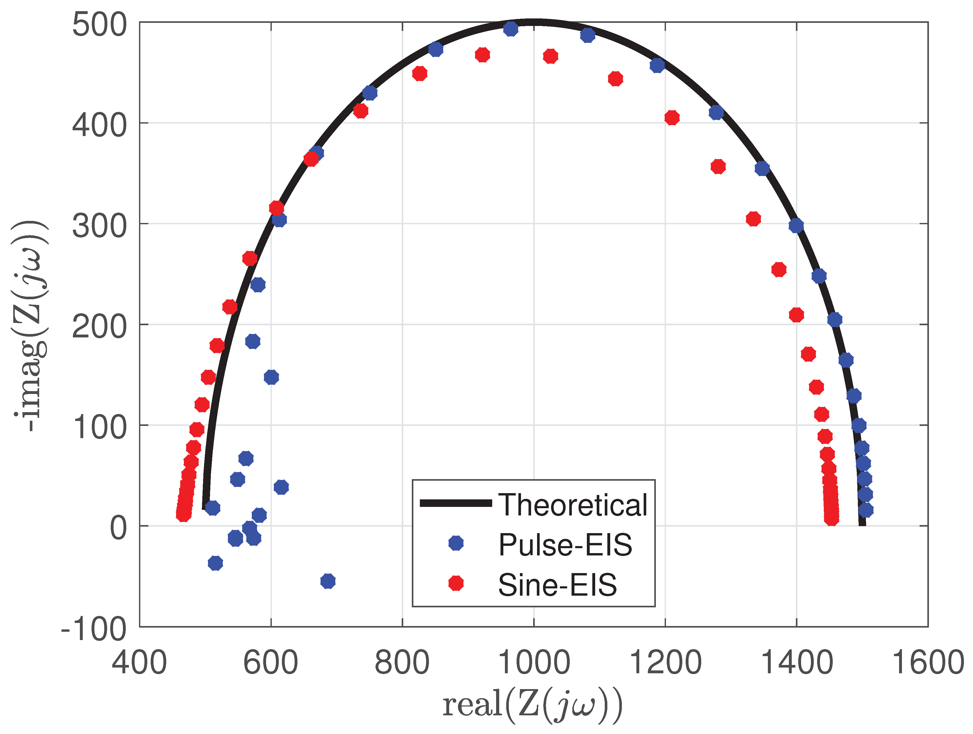
Figure 16 shows the pulse-EIS in comparison to the state-of-the-art EIS using sinusoidal signals, and the theoretical plot. The state-of-the-art EIS response is obtained using the Gamry interface 5000P, by exciting the RC circuit using sinusoidal signals of frequencies 0.01Hz to 100 Hz.
7. Conclusion
The key findings of the paper are summarized below,
- There is a rule of thumb to selecting the sampling time: The sampling time, , should be chosen to be less than atleast one-tenth of the system’s minimum time constant i.e., .
- There is a rule of thumb for the excitation pulse design: The pulse excitation signal comprises a non-zero portion lasting and a zero portion lasting . A general rule of thumb for selecting these durations is to set approximately equal to the minimum time constant, i.e., of the system, and approximately ten times the maximum time constant, i.e., .
- Noise can be reduced through averaging: This paper demonstrated that the measurement noise in both voltage and current signals retains its zero-mean property after applying the discrete Fourier transform, enabling effective noise reduction through averaging.
- Zero-padding improves resolution: When a pulse excitation signal is used, the resulting responses are unevenly distributed across the frequency domain, with a higher concentration appearing in the high-frequency region. To improve resolution in the low-frequency range, zero-padding is applied. While zero-padding also increases resolution in the high-frequency region, responses from closely spaced frequencies can be grouped and averaged to reduce noise. This approach leads to a more balanced spectral distribution.
Author contributions: Conceptualization, B.B. and K.R.P.; methodology, B.B. and S.S.; software, S.S.; validation, S.S.; formal analysis, S.S.; data curation, S.S.; writing—original draft preparation, S.S.; writing—review and editing, B.B., K.R.P., S.S., ; visualization, S.S.; supervision, B.B.; project administration, B.B.; funding acquisition, B.B.
Funding: This research was funded by Natural Sciences and Engineering Research Council of Canada (NSERC) grant number RGPIN-2024-04557.
Conflicts of Interest: The authors declare no conflict of interest. The funders had no role in the design of the study; in the collection, analyses, or interpretation of data; in the writing of the manuscript; or in the decision to publish the results.
Appendix A. DFT of Excitation Signal
For the signal defined in (2), the DFT is,
For ,
Appendix B. Mean of the Transformed Voltage and Current Noise
The DFT of the voltage noise is shown in (11). Considering voltage noise at the frequency bin to be denoted by , we have
The mean of the transformed voltage noise, given is assumed to be zero-mean noise, is
Similarly, it can be shown that the zero-mean property is preserved in the transformed current noise.
References
- Chen, H.; Bai, J.; Wu, Z.; Song, Z.; Zuo, B.; Fu, C.; Zhang, Y.; Wang, L. Rapid impedance measurement of Lithium-Ion batteries under pulse ex-citation and analysis of impedance characteristics of the regularization distributed relaxation time. Batteries 2025, 11, 91. [Google Scholar] [CrossRef]
- Nunes, H.; Martinho, J.; Fermeiro, J.; Pombo, J.; Mariano, S.; do Rosário Calado, M. Impedance analysis and parameter estimation of lithium-ion batteries using the eis technique. IEEE Transactions on Industry Applications 2024. [Google Scholar] [CrossRef]
- Meddings, N.; Heinrich, M.; Overney, F.; Lee, J.S.; Ruiz, V.; Napolitano, E.; Seitz, S.; Hinds, G.; Raccichini, R.; Gaberšček, M.; et al. Application of electrochemical impedance spectroscopy to commercial Li-ion cells: A review. Journal of Power Sources 2020, 480, 228742. [Google Scholar] [CrossRef]
- Messing, M.; Shoa, T.; Ahmed, R.; Habibi, S. Battery SoC estimation from EIS using neural nets. In Proceedings of the 2020 IEEE transportation electrification conference &, 2020, expo (ITEC). IEEE; pp. 588–593.
- Bourelly, C.; Vitelli, M.; Milano, F.; Molinara, M.; Fontanella, F.; Ferrigno, L. Eis-based soc estimation: A novel measurement method for optimizing accuracy and measurement time. IEEE Access 2023, 11, 91472–91484. [Google Scholar] [CrossRef]
- Li, C.; Yang, L.; Li, Q.; Zhang, Q.; Zhou, Z.; Meng, Y.; Zhao, X.; Wang, L.; Zhang, S.; Li, Y.; et al. SOH estimation method for lithium-ion batteries based on an improved equivalent circuit model via electrochemical impedance spectroscopy. Journal of Energy Storage 2024, 86, 111167. [Google Scholar] [CrossRef]
- Zhou, Z.; Li, Y.; Wang, Q.G.; Yu, J. Health indicators identification of lithium-ion battery from electrochemical impedance spectroscopy using geometric analysis. IEEE Transactions on Instrumentation and Measurement 2023, 72, 1–9. [Google Scholar] [CrossRef]
- Teliz, E.; Zinola, C.F.; Díaz, V. Identification and quantification of ageing mechanisms in Li-ion batteries by Electrochemical impedance spectroscopy. Electrochimica Acta 2022, 426, 140801. [Google Scholar] [CrossRef]
- Fu, Y.; Xu, J.; Shi, M.; Mei, X. A fast impedance calculation-based battery state-of-health estimation method. IEEE Transactions on Industrial Electronics 2021, 69, 7019–7028. [Google Scholar]
- Li, A.G.; West, A.C.; Preindl, M. Characterizing degradation in lithium-ion batteries with pulsing. Journal of Power Sources 2023, 580, 233328. [Google Scholar] [CrossRef]
- Guha, A.; Patra, A. Online Estimation of the Electrochemical Impedance Spectrum and Remaining Useful Life of Lithium-Ion Batteries. IEEE Transactions on Instrumentation and Measurement 2018, 67, 1836–1849. [Google Scholar] [CrossRef]
- Wu, Y.; Sundaresan, S.; Balasingam, B. Battery parameter analysis through electrochemical impedance spectroscopy at different state of charge levels. Journal of Low Power Electronics and Applications 2023, 13, 29. [Google Scholar] [CrossRef]
- Abaspour, M.; Pattipati, K.R.; Shahrrava, B.; Balasingam, B. Robust approach to battery equivalent-circuit-model parameter extraction using electrochemical impedance spectroscopy. Energies 2022, 15, 9251. [Google Scholar] [CrossRef]
- Srinivasan, R.; Fasmin, F. An introduction to electrochemical impedance spectroscopy; CRC Press, 2021.
- Pérez, G.; Gandiaga, I.; Garmendia, M.; Reynaud, J.; Viscarret, U. Modelling of Li-ion batteries dynamics using impedance spectroscopy and pulse fitting: EVs application. In Proceedings of the 2013 World Electric Vehicle Symposium and Exhibition (EVS27). IEEE; 2013; pp. 1–9. [Google Scholar]
- Schmidt, J.P.; Ivers-Tiffée, E. Pulse-fitting–A novel method for the evaluation of pulse measurements, demonstrated for the low frequency behavior of lithium-ion cells. Journal of Power Sources 2016, 315, 316–323. [Google Scholar]
- Kollmeyer, P.; Hackl, A.; Emadi, A. Li-ion battery model performance for automotive drive cycles with current pulse and EIS parameterization. In Proceedings of the 2017 IEEE transportation electrification conference and expo (ITEC). IEEE; 2017; pp. 486–492. [Google Scholar]
- Tang, X.; Lai, X.; Liu, Q.; Zheng, Y.; Zhou, Y.; Ma, Y.; Gao, F. Predicting battery impedance spectra from 10-second pulse tests under 10 Hz sampling rate. IScience 2023, 26. [Google Scholar]
- Li, A.G.; Fahmy, Y.A.; Wu, M.M.; Preindl, M. Fast time-domain impedance spectroscopy of lithium-ion batteries using pulse perturbation. In Proceedings of the 2022 IEEE Transportation Electrification Conference &, 2022, Expo (ITEC). IEEE; pp. 155–160.
- Wang, L.; Song, Z.; Zhu, L.; Jiang, J. Fast electrochemical impedance spectroscopy of lithium-ion batteries based on the large square wave excitation signal. IScience 2023, 26. [Google Scholar]
- Boškoski, P.; Debenjak, A.; Mileva Boshkoska, B.; Boškoski, P.; Debenjak, A.; Mileva Boshkoska, B. Fast electrochemical impedance spectroscopy; Springer, 2017.
- Gabrielli, C.; Huet, F.; Keddam, M.; Lizee, J. Measurement time versus accuracy trade-off analyzed for electrochemical impedance measurements by means of sine, white noise and step signals. Journal of electroanalytical chemistry and interfacial electrochemistry 1982, 138, 201–208. [Google Scholar] [CrossRef]
- Duhamel, P.; Vetterli, M. Fast Fourier transforms: a tutorial review and a state of the art. Signal processing 1990, 19, 259–299. [Google Scholar] [CrossRef]
- Takano, K.; Nozaki, K.; Saito, Y.; Kato, K.; Negishi, A. Impedance Spectroscopy by Voltage-Step Chronoamperometry Using the Laplace Transform Method in a Lithium-Ion Battery. Journal of The Electrochemical Society 2000, 147, 922. [Google Scholar] [CrossRef]
- Onda, K.; Nakayama, M.; Fukuda, K.; Wakahara, K.; Araki, T. Cell impedance measurement by Laplace transformation of charge or discharge current–voltage. Journal of the Electrochemical Society 2006, 153, A1012. [Google Scholar] [CrossRef]
- Li, T.; Wang, D.; Wang, H. New method for acquisition of impedance spectra from charge/discharge curves of lithium-ion batteries. Journal of Power Sources 2022, 535, 231483. [Google Scholar] [CrossRef]
- Wang, X.; Kou, Y.; Wang, B.; Jiang, Z.; Wei, X.; Dai, H. Fast Calculation of Broadband Battery Impedance Spectra Based on S Transform of Step Disturbance and Response. IEEE Transactions on Transportation Electrification 2022, 8, 3659–3672. [Google Scholar] [CrossRef]
- Li, W.; Huang, Q.A.; Yang, C.; Chen, J.; Tang, Z.; Zhang, F.; Li, A.; Zhang, L.; Zhang, J. A fast measurement of Warburg-like impedance spectra with Morlet wavelet transform for electrochemical energy devices. Electrochimica Acta 2019, 322, 134760. [Google Scholar] [CrossRef]
- Hoshi, Y.; Yakabe, N.; Isobe, K.; Saito, T.; Shitanda, I.; Itagaki, M. Wavelet transformation to determine impedance spectra of lithium-ion rechargeable battery. Journal of Power Sources 2016, 315, 351–358. [Google Scholar] [CrossRef]
- Itagaki, M.; Ueno, M.; Hoshi, Y.; Shitanda, I. Simultaneous determination of electrochemical impedance of lithium-ion rechargeable batteries with measurement of charge-discharge curves by wavelet transformation. Electrochimica Acta 2017, 235, 384–389. [Google Scholar] [CrossRef]
- Lohmann, N.; Weßkamp, P.; Haußmann, P.; Melbert, J.; Musch, T. Electrochemical impedance spectroscopy for lithium-ion cells: Test equipment and procedures for aging and fast characterization in time and frequency domain. Journal of Power Sources 2015, 273, 613–623. [Google Scholar] [CrossRef]
- Balasingam, B. Robust Battery Management System Design With MATLAB; Artech House, 2023.
- Kuo, B.C. Automatic control systems; Prentice Hall PTR, 1987.
- Sundaresan, S.; Pattipati, K.; Balasingam, B. Fast Electrochemical Impedance Spectroscopy for Battery Testing. IEEE International Symposium on Industrial Electronics.
Figure 1.
Current excitation & voltage response
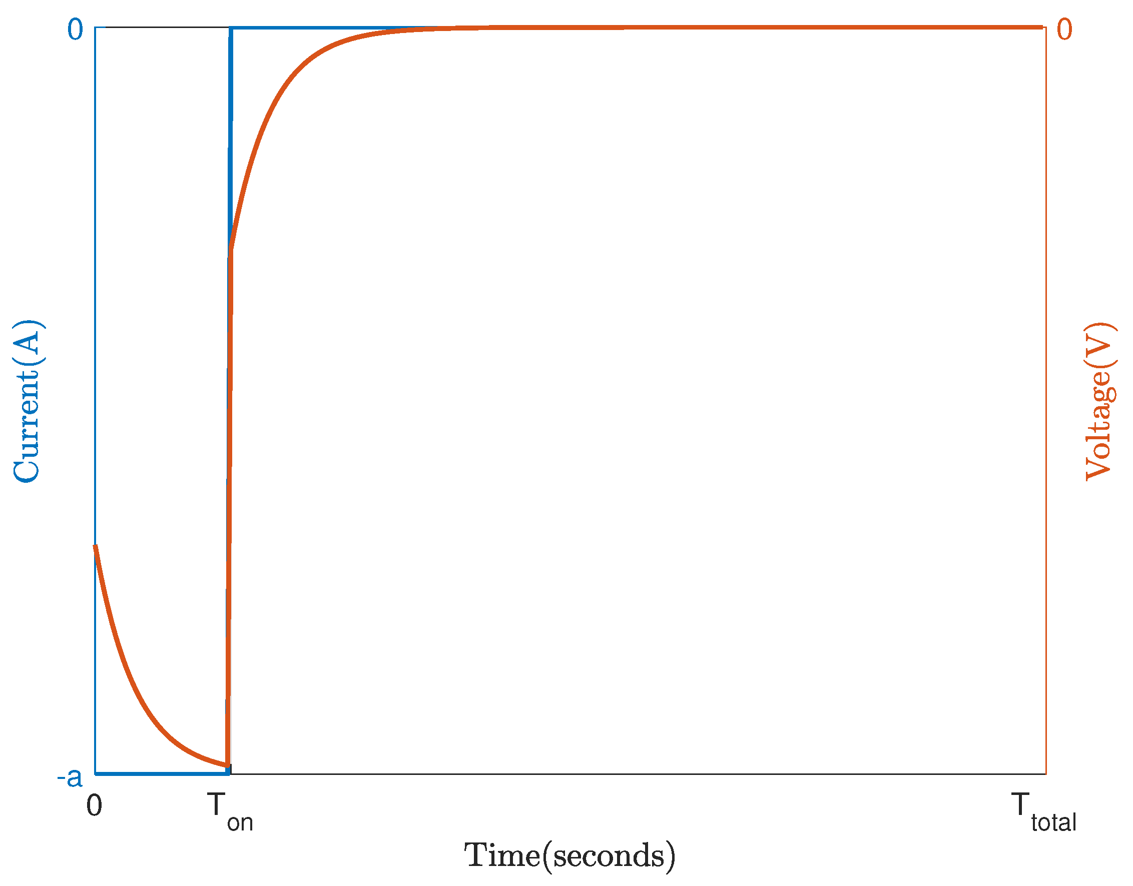
Figure 2.
Equivalent circuit model of the battery with highlighted components
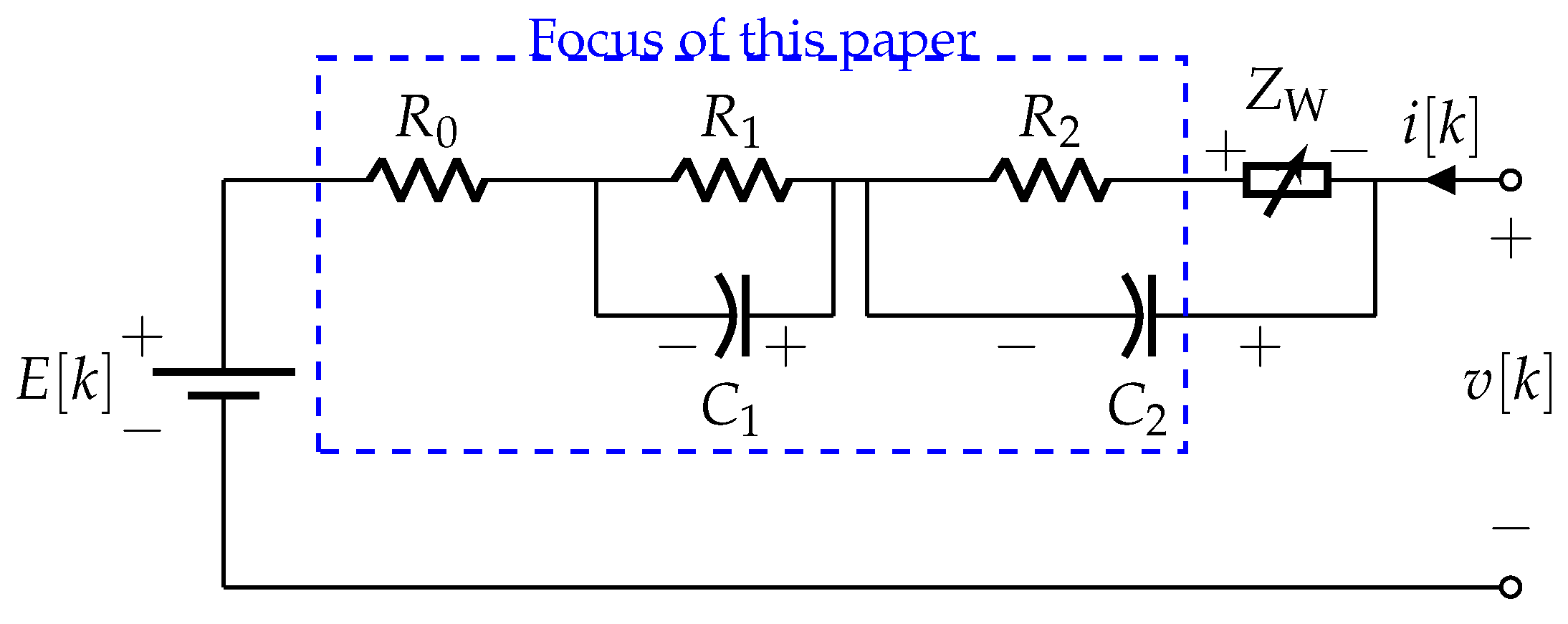
Figure 3.
Typical Nyquist plot of a battery
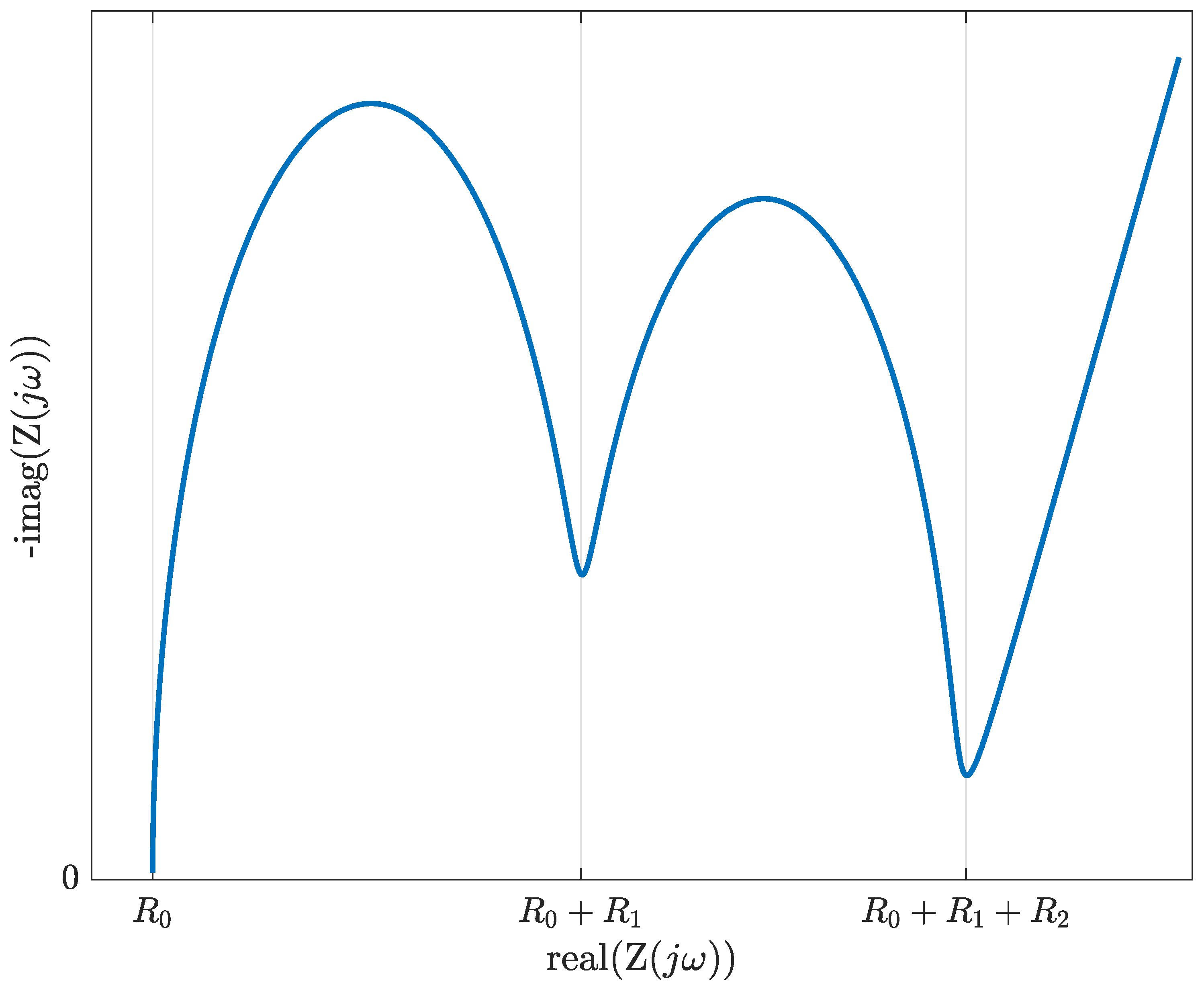
Figure 4.
Discrete rectangular pulse excitation signal
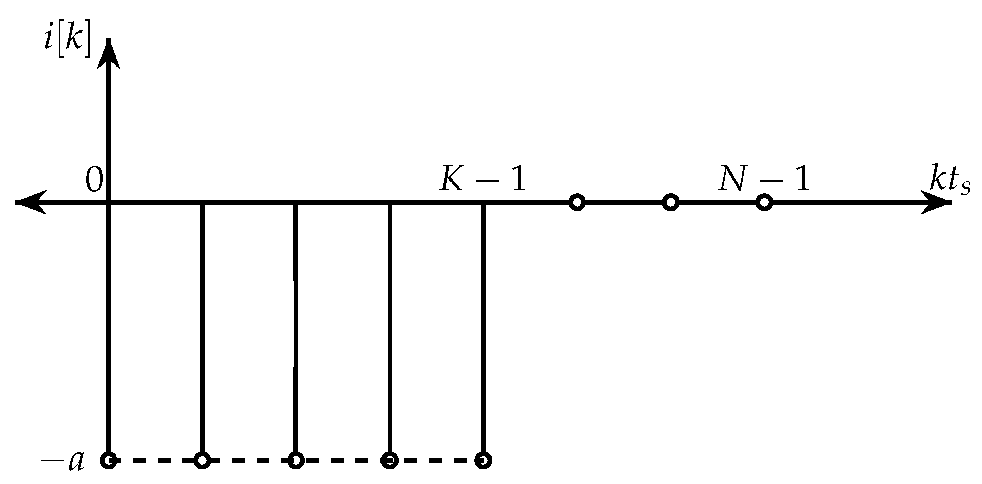
Figure 5.
Frequency response of the RC-circuit
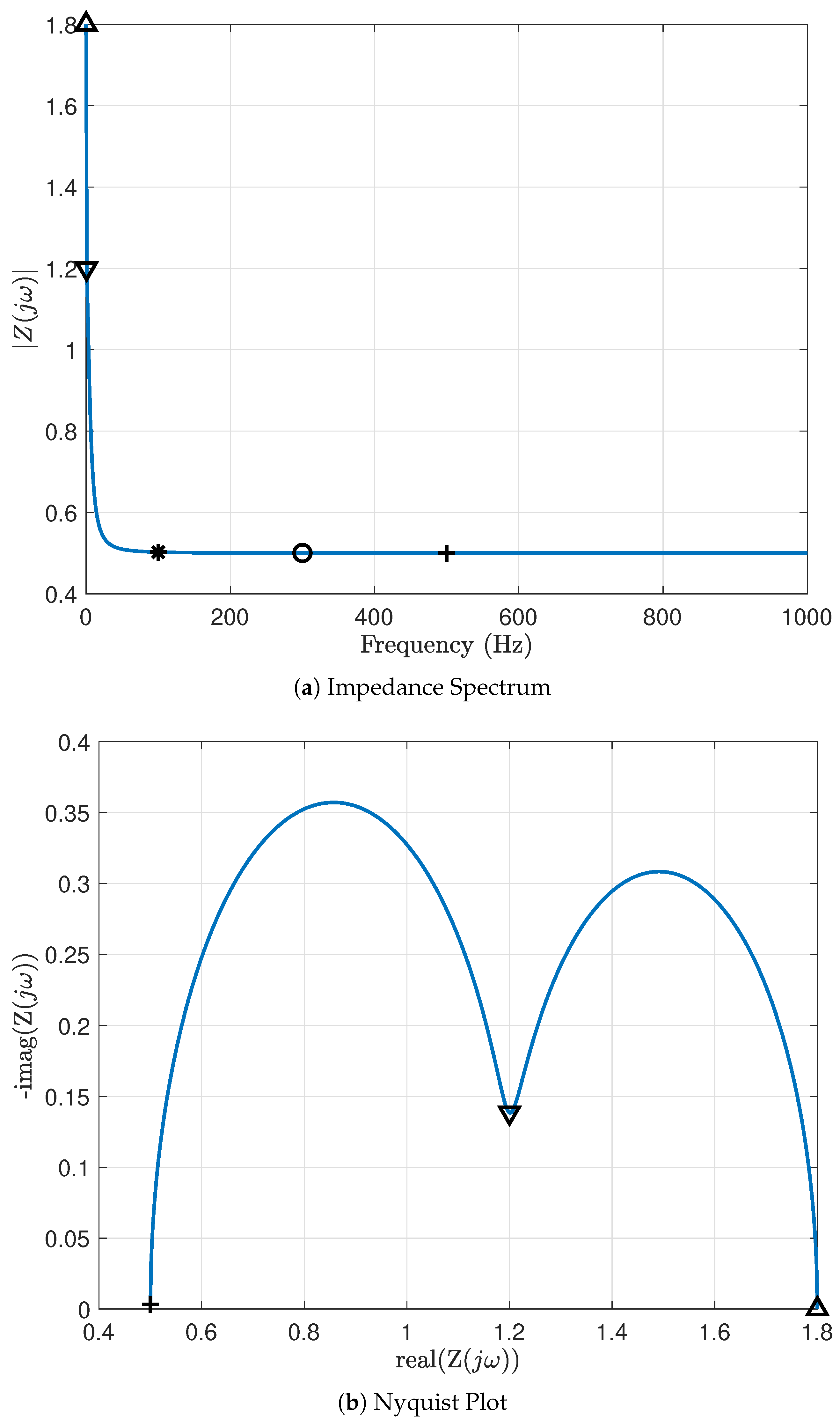
Figure 6.
Nyquist response for varying values
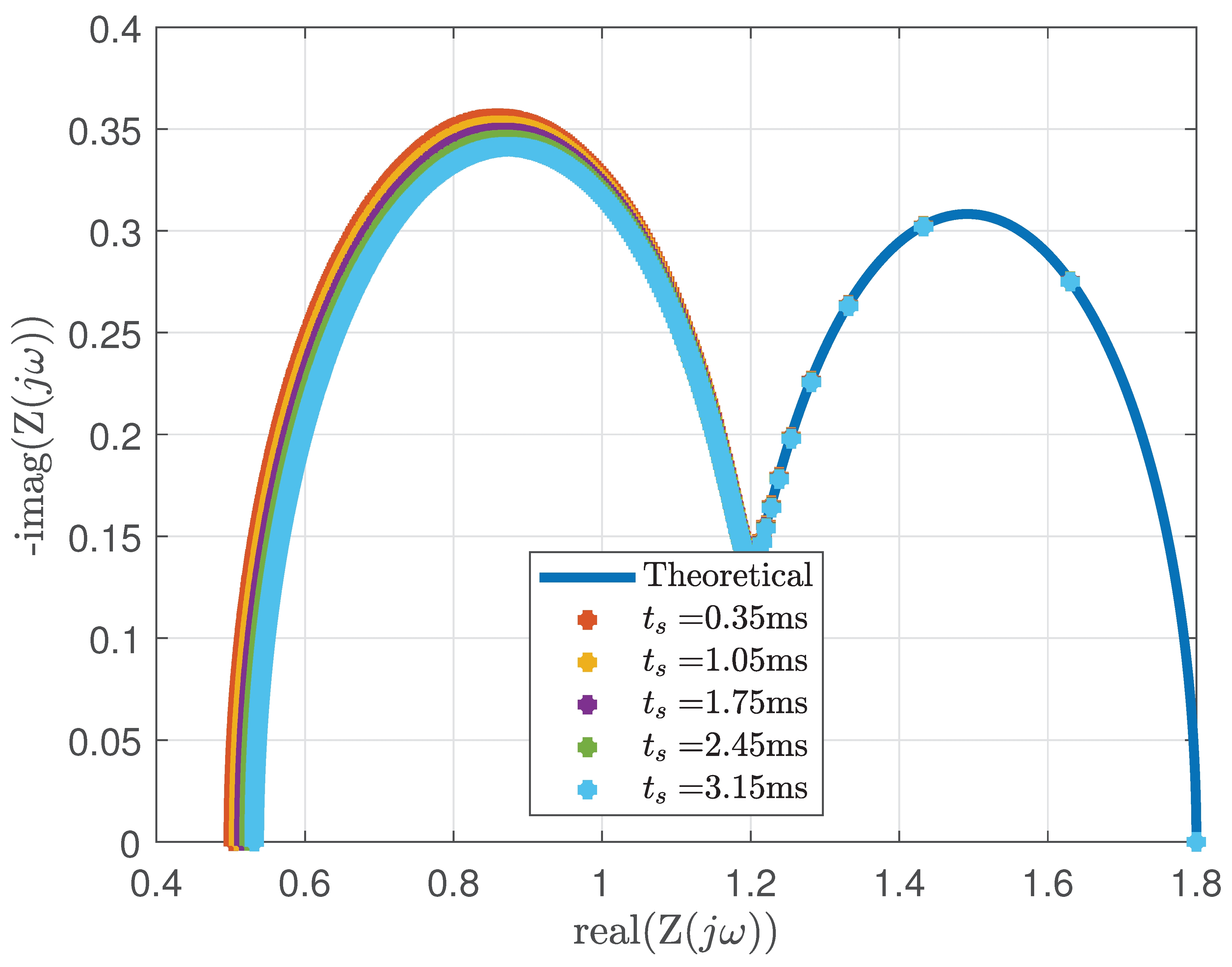
Figure 7.
Error metrics for varying values
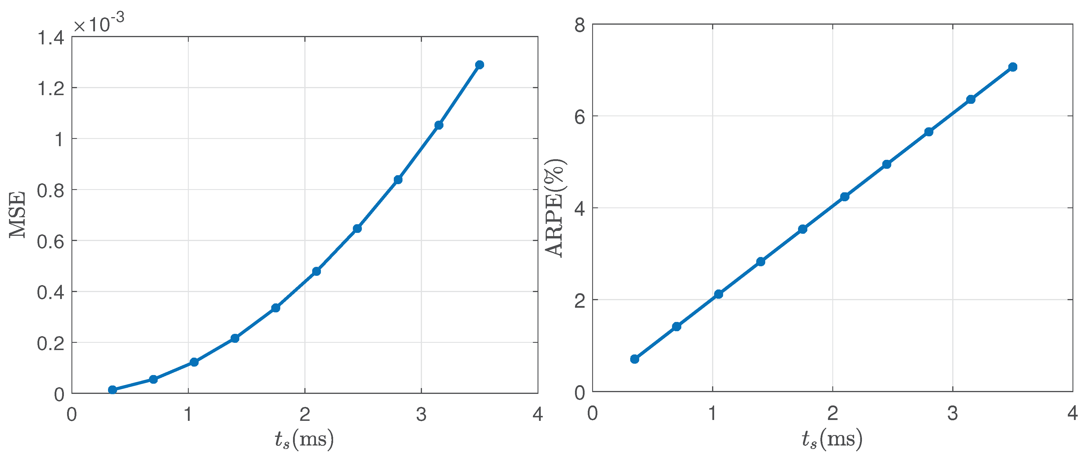
Figure 8.
Excitation & response spectra for varying values
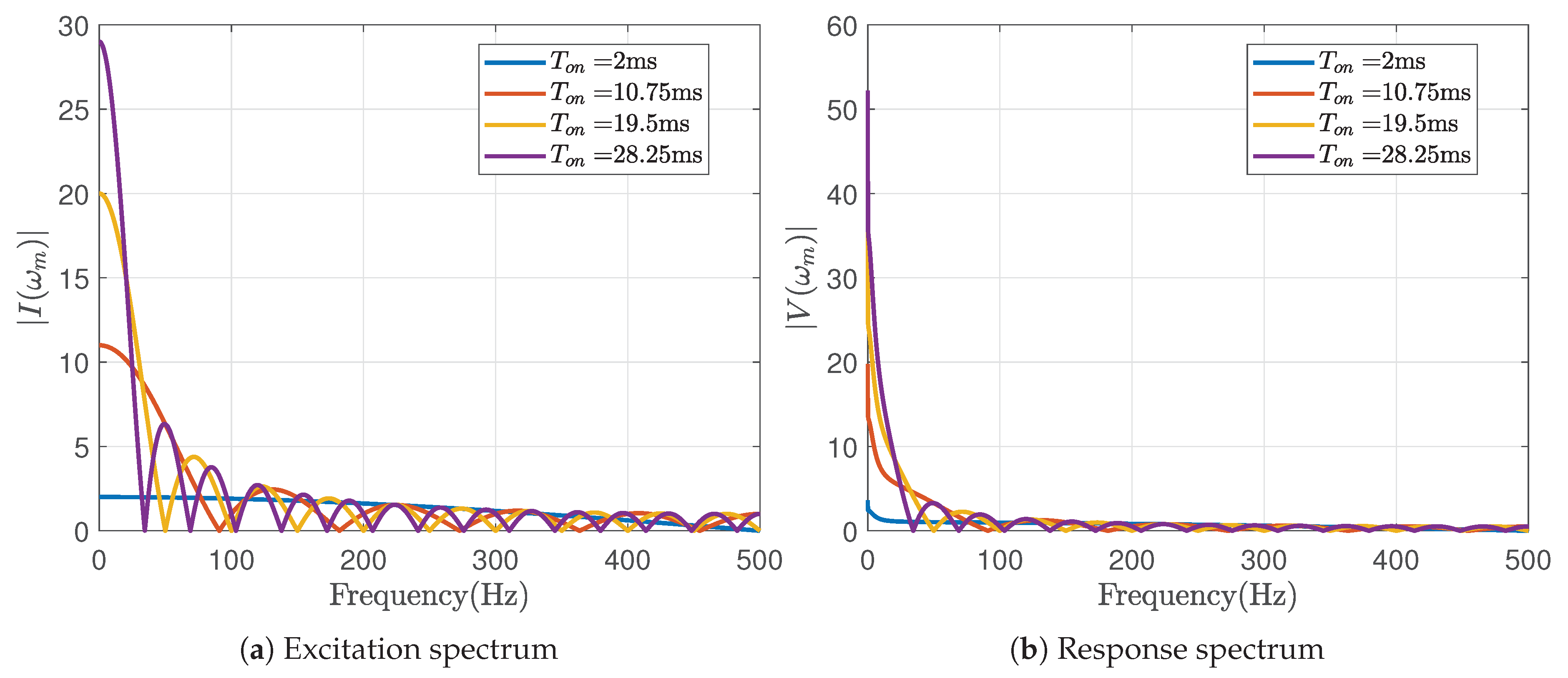
Figure 9.
Nyquist response for varying values
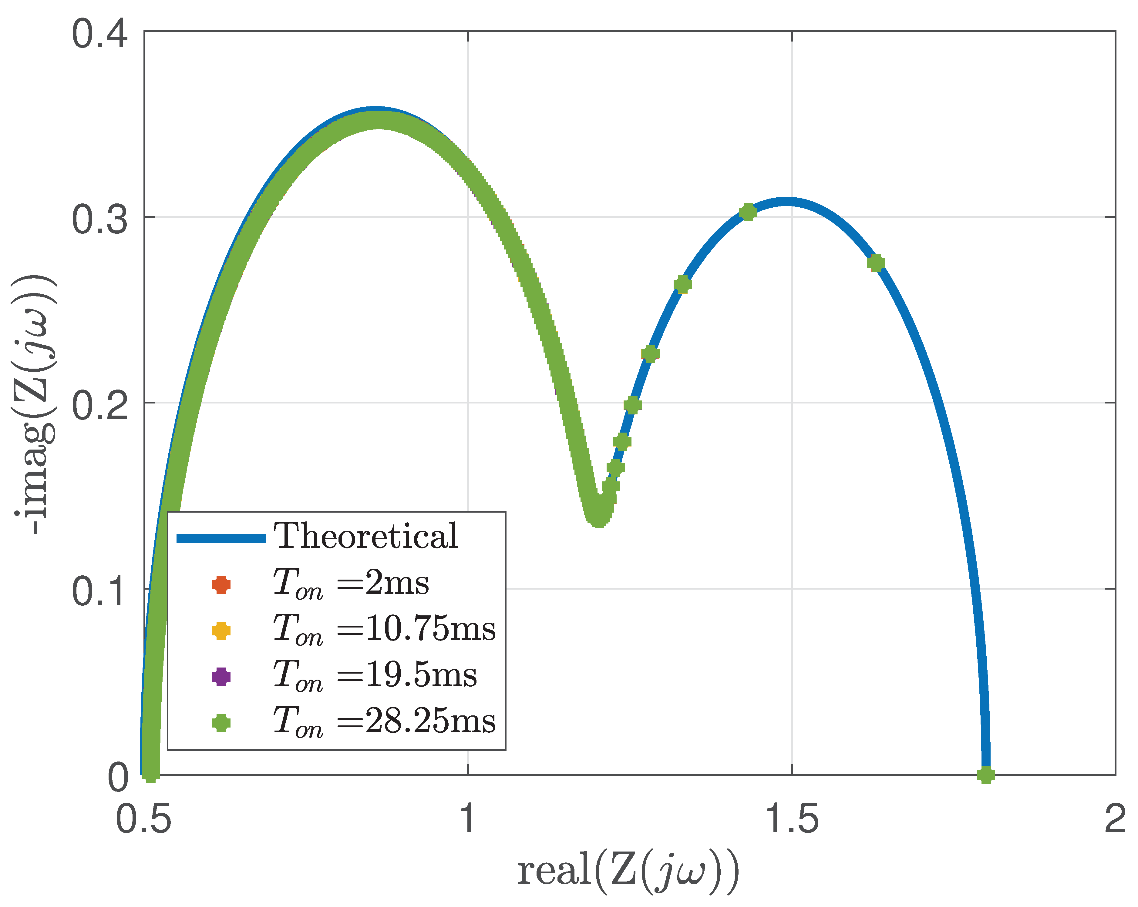
Figure 10.
Effects of zero-padding on the Nyquist plot
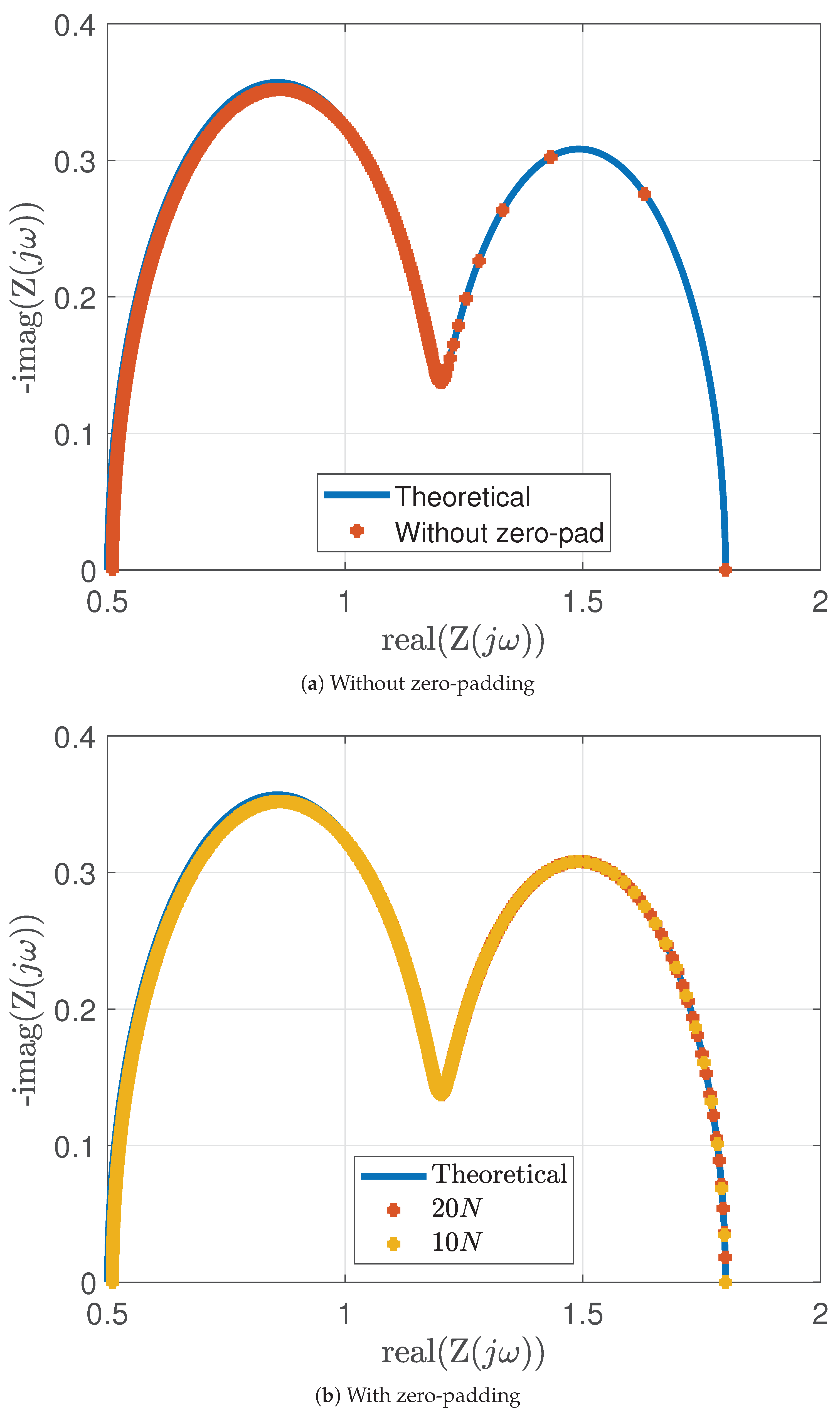
Figure 11.
Error metrics with varying
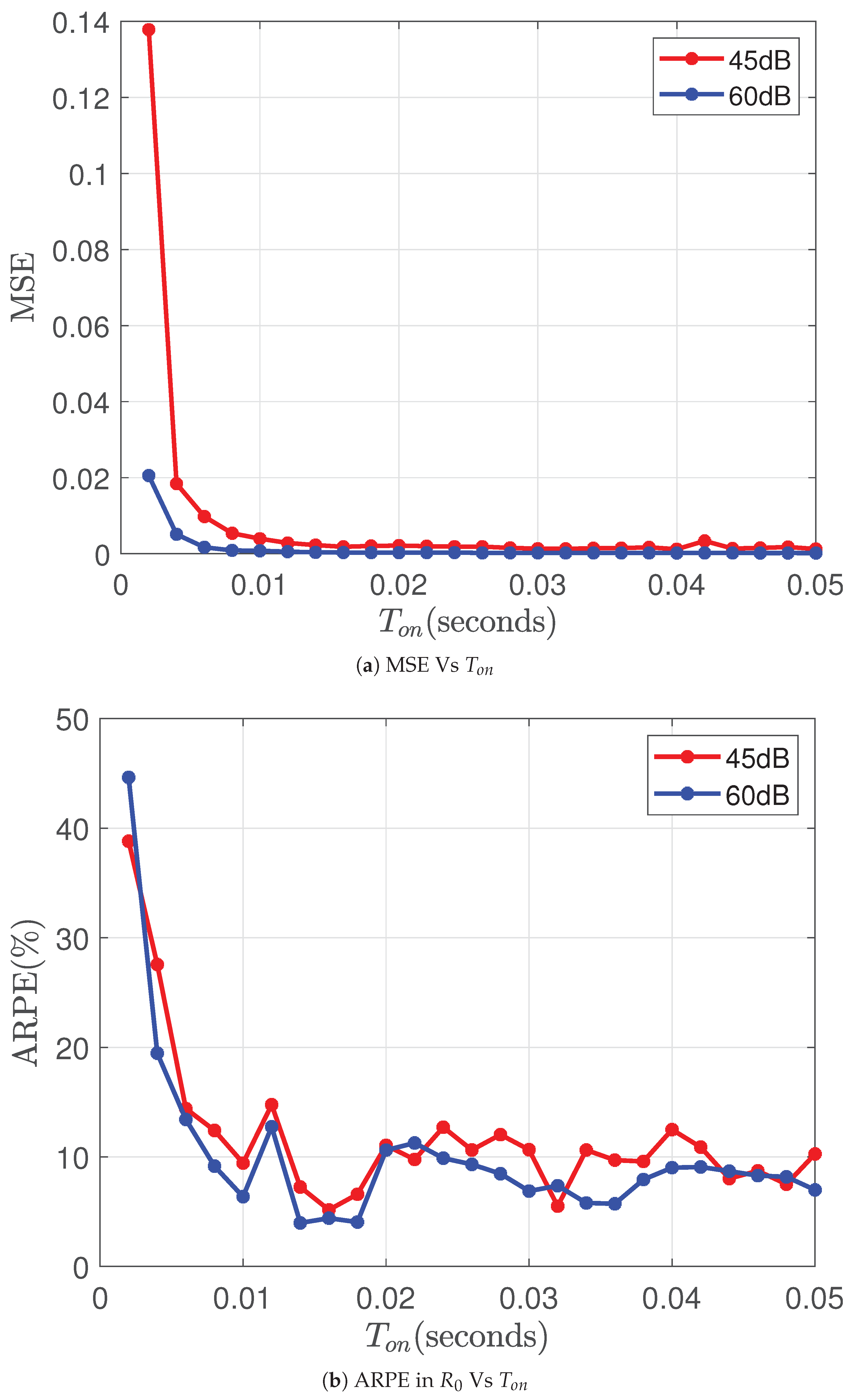
Figure 12.
1-RC experimental setup
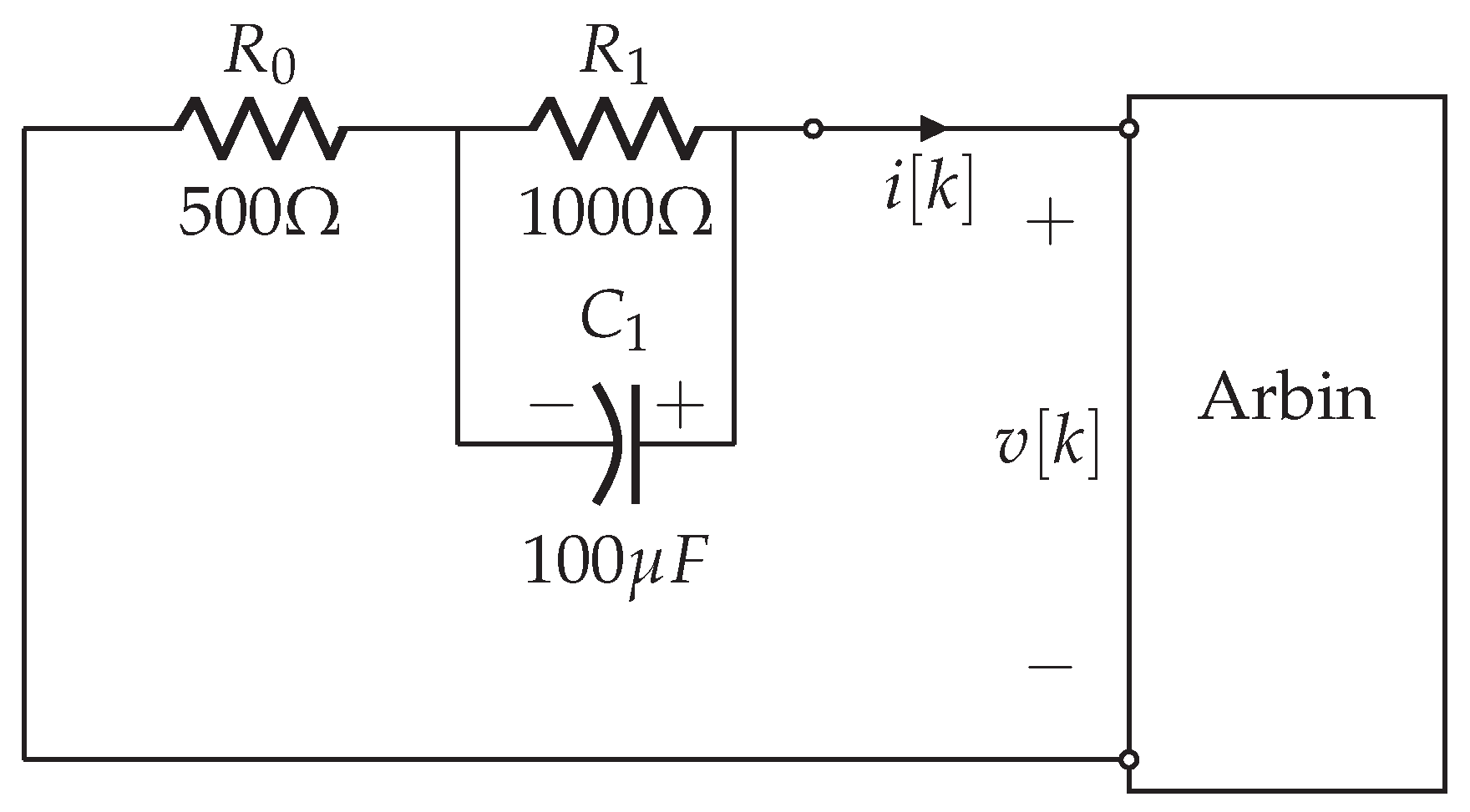
Figure 13.
V-I data from the 1-RC circuit
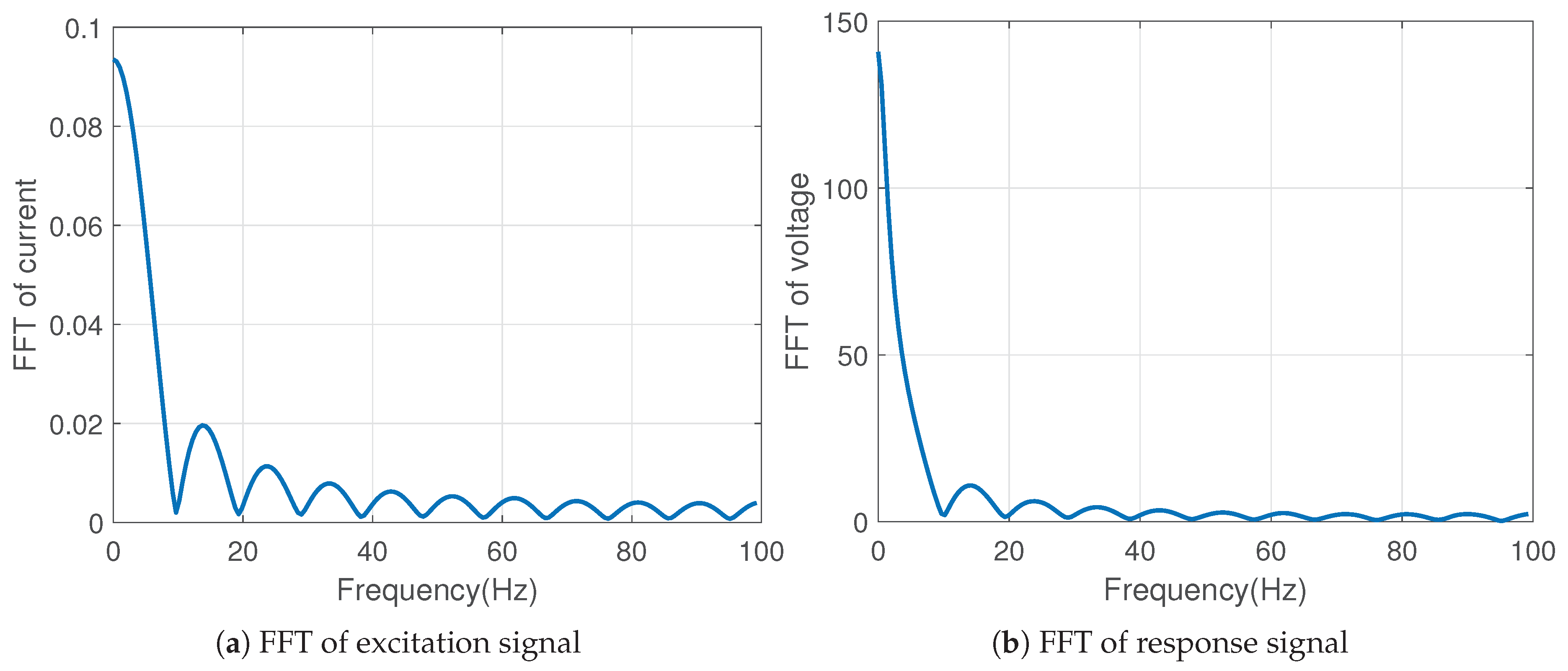
Figure 14.
Excitation and response spectra
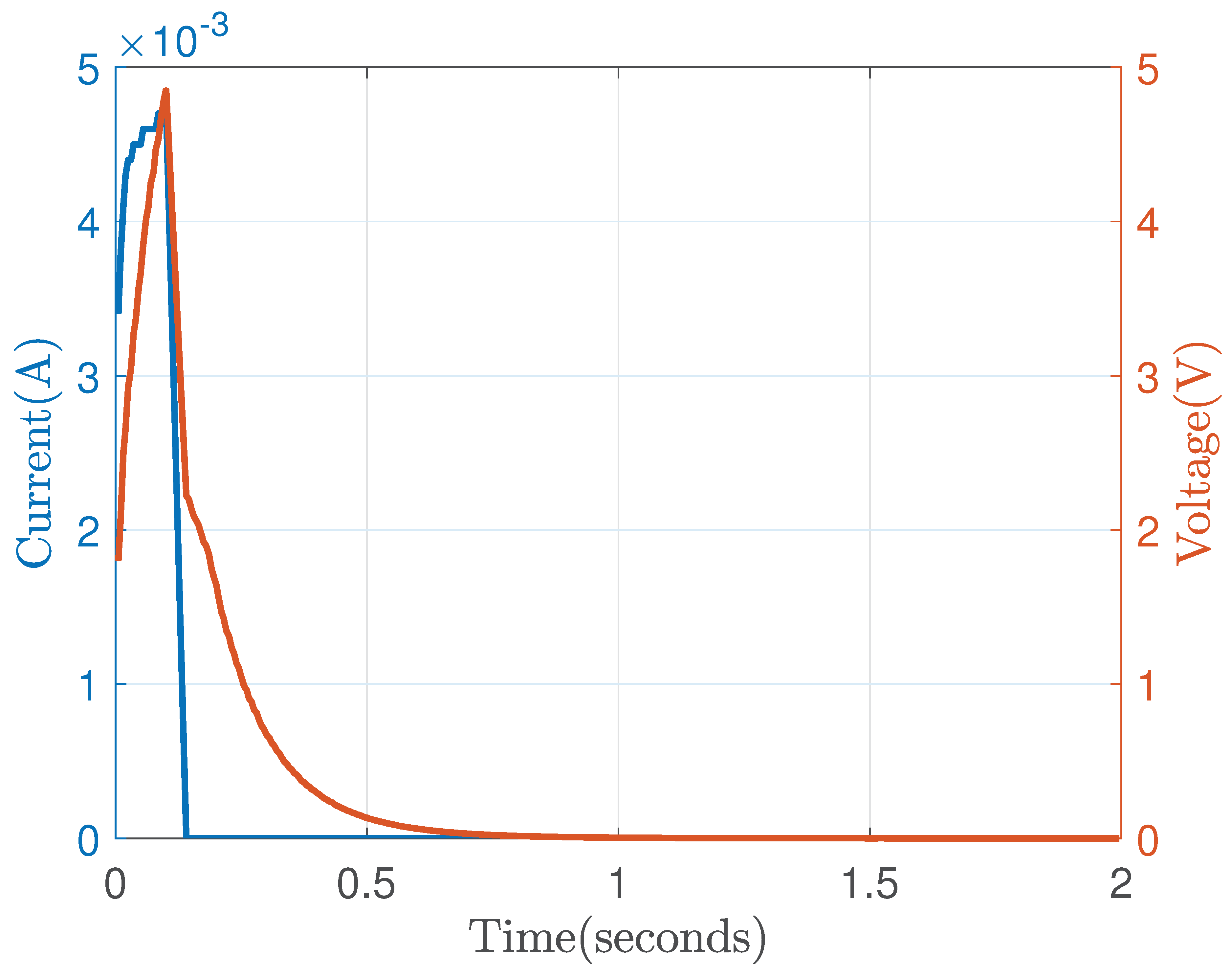
Figure 15.
Pulse-EIS for the 1-RC circuit
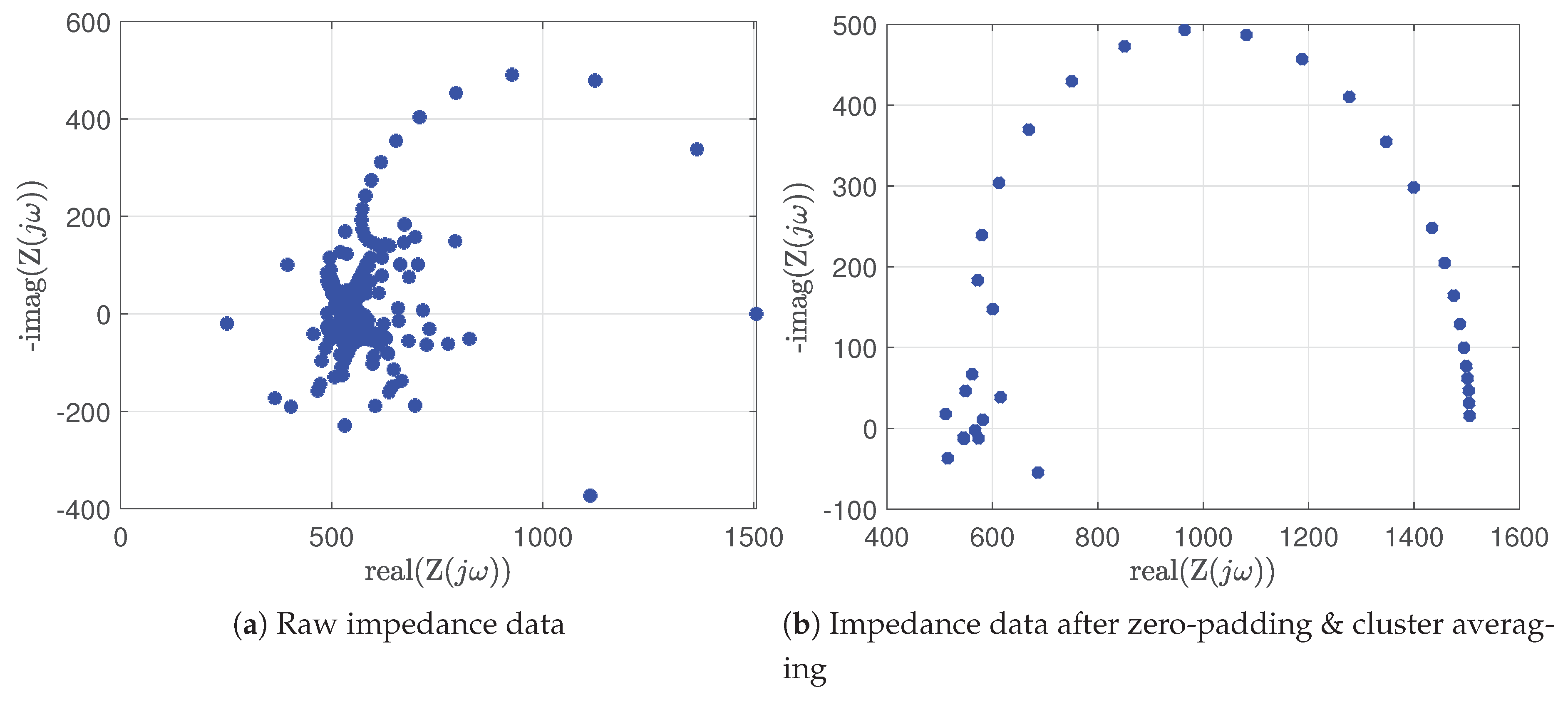
Figure 16.
Comparison of the Nyquist plots
Disclaimer/Publisher’s Note: The statements, opinions and data contained in all publications are solely those of the individual author(s) and contributor(s) and not of MDPI and/or the editor(s). MDPI and/or the editor(s) disclaim responsibility for any injury to people or property resulting from any ideas, methods, instructions or products referred to in the content. |
© 2025 by the authors. Licensee MDPI, Basel, Switzerland. This article is an open access article distributed under the terms and conditions of the Creative Commons Attribution (CC BY) license (https://creativecommons.org/licenses/by/4.0/).
Copyright: This open access article is published under a Creative Commons CC BY 4.0 license, which permit the free download, distribution, and reuse, provided that the author and preprint are cited in any reuse.


