
Submitted:
05 February 2025
Posted:
05 February 2025
You are already at the latest version
Abstract
The galvanostatic intermittent titration technique (GITT) was applied to NMC622 positive electrodes, with Electrochemical Impedance Spectroscopy (EIS) performed at quasi-equilibrium conditions determined by cutoff criteria based on relaxation rates. Below an open-circuit voltage (OCV) of 3.8 V, the cutoff criterion of 0.1 mV h−1 was reached after approximately 8 hours. However, above 3.8 V, a non-saturating voltage decay was observed, increasing up to ∼0.56 mV h−1 above 4.1 V during charging steps. This persistent voltage decay upon subsequent discharging steps led to non-monotonic relaxation behavior. A pulse time of 10 minutes did not satisfy the t dependence required for GITT kinetic analysis. Instead, the initial 36-second transients were extended for chemical diffusivity evaluation, aligning with the Warburg-like response observed in EIS, consistent with the sequential reaction-diffusion assumption. GITT analysis for solid-state diffusivity is ineffective for spherical active particles dispersed in porous electrodes and performs even worse due to liquid-phase diffusion within the pores, where t+=0.3. The apparent SOC-independent chemical diffusivity obtained from GITT across both low and high OCV ranges suggests that the process is dominated by liquid-phase diffusion. The application of the physics-based three-rail transmission line model (TLM) developed by Gaberšček et al. in EIS holds practical potential for deconvoluting the two diffusion kinetics.
Keywords:
GITT
; EIS
; spherical diffusion
; chemical diffusivity
; relaxation
; pulse times
; short-time solution
; 3-rail transmission line model
; liquid phase diffusion
; transference number
1. Introduction
Introduced by Weppner and Huggins [1], the Galvanostatic Intermittent Titration Technique (GITT) has gained widespread acceptance to assess chemical diffusivity in battery electrode materials as a function of state-of-charge (SOC). Currently, there are several issues in conventional practices.
- Relaxation periods are set to constant, e.g., 1 h, in automated procedures provided by the commercial potentio/galvanostats, are not likely to reach equilibrium OCVs, which is one of the main purposes of GITT.
- The titration pulse should be short enough for the square root-of-time-dependent solution of the diffusion equation [1,2]. Conventionally, the entire SOC range of the layered oxide electrodes, which is assumed to be a solid solution, is titrated. With the 0.1C current, the pulse duration 1 h makes 10 steps, 10 min 60 steps, and 1 min 600 steps. In most studies, the pulse duration is not short enough.
- Original GITT kinetic analysis is for thin-film electrodes. The applicability to the spherical active material particles dispersed in porous electrodes is questioned. EIS employing a physics-based equivalent circuit model, recently developed by Gaberšček et al., has the practical potential to properly determine chemical diffusivity. [3,4,5,6,7].
In the present work, GITT and EIS are combined for the thermodynamic and kinetic properties of LiNi0.6Mn0.2Co0.2O2, NMC622. When equilibrium OCV is reached after each titration step, EIS is measured, which can be compared to the voltage transients upon the following current pulse for the GITT kinetic analysis for chemical diffusivity. Sufficiently long relaxation periods were assured to reach quasi-equilibrium.
2. Experimental
Commercial powder (NMC622, Umicore) with an average size 5.07±0.97 m, determined by SEM, was thoroughly mixed with conductive carbon black (EQ-lib-Super65, MTI) and polyvinylidene fluoride (PVDF; Mv = 600,000, MTI) binder in N-Methyl-2-pyrrolidone (NMP; 99%, Sigma-Aldrich), in a weight ratio of 8:1:1, respectively. This mixture was then uniformly coated on aluminum foil using a doctor blade of 180 m thickness. Subsequently, the coated foil was dried under vacuum at 80 ∘C for 12 h. Afterward, the dried electrode was punched into discs with a diameter of 14 mm. A 16 mm in diameter lithium chip was used as the reference and counter electrode. Each cell is configured in a CR2032 coin cell with a working electrode, a separator (3501, Celgard®, 25m), and a lithium electrode. A 50 l of electrolyte containing 1 M lithium hexafluorophosphate (LiPF6; 99,99%, Sigma-Aldrich) in ethylene carbonate (EC; 98%, Sigma-Aldrich) and dimethyl carbonate (DMC; 99%, Sigma-Aldrich) in a 1:1 volume ratio, respectively, was subsequently introduced into the separator. All cell fabrication procedures were performed in an argon-filled glovebox. The cells manufactured were aged at 25∘C for 18 h prior to electrochemical testing.
The amount of active material in a cell was approximately 3 mg, and the capacity value for the calculation of the C rate was assumed to be 180 mAhg−1 [8,9]. The coin cells were loaded into a Peltier chamber (Memmert IPP30plus, Germany) set at 30∘C using a 10-coin cell holder (Neoscience, Korea). The temperature variation of the cell during battery testing was continuously measured using K-type thermocouples attached directly at the top of the cells. Electrochemical measurements were made using Biologic software (VSP300, France) using the dedicated EC-Lab software®.
For clarity, large data in Figures were presented by utilizing data distance threshold skip method of OriginLab® 2023 (OriginLab Corporation, Northampton, MA, USA). Impedance analysis and simulation were made using ZView® (Scribner Ass. Inc., USA) and Python codes updated from one provided by Prof. Miran Gaberšček, National Institute of Chemistry, Ljubljana, Slovenia, in 2023, June.
3. Formation Cycles
Ten consecutive charge-discharge cycles stabilized fresh cells at 0.1 C rate between 2.5 V and 4.3 V, Figure 1. The first charging typically shows a high capacity, 200 mAhg−1, which can be attributed to SEI formation, and the capacity stabilized close to the nominal value of 180 mAhg−1, Figure 1(a). The differential capacity curves in Figure 1(b) clearly show the asymmetry between the charging and discharging. Two split peaks in charge and single peaks in discharge are characteristic of the high-nickel composition above 622 [10,11]. While charging starts above 3.7V, discharging gradually decreases below the peak of around 3.7V.
The setup in this work monitored the temperature of each battery cell in situ, Figure 1(c). For the coin cells, endothermic/exothermic heat effects upon charging/discharging and Joule heating are very small to be distinguished from the noise. Endothermic heat effects due to SEI formation were observed in the first charging cycles. The observation supports the application of three to five SEI formation cycles. The decomposition of solvent molecules may explain the endothermicity of the SEI formation reaction.
4. GITT: Overview
Figure 2 shows the raw data of GITT as a function of time, left, and the state of charge, right. Pulses 54.4 A corresponding to 0.1 C were applied for the active material 3.02 mg for 10 min, and the relaxation to equilibrium was manually controlled to meet the criteria mV h−1 or mV h−1, Figure 3 and Figure 4, detailed in the next section. After reaching equilibrium criteria, EIS was measured with an AC voltage of 10 mV to OCV from 1 MHz to 10 mHz. Then the next titration pulse was applied. The voltage measurement intervals were changed from 1 s during the pulse to 10 s for the first hour of relaxation and 60 s afterward. The cutoff was set from 2.5 to 4.2 V, but stable OCV for GITT can be achieved above 3.6 V, as shown.
5. GITT for Equilibrium OCVs
GITT for a charging and discharging cycle in Figure 2 took more than two months, and the degradation or time-dependent change is likely in the cell components: electrolyte, lithium reference electrode as well as the NMC622 electrode. It is shown that the capacity fades from 180 mAhg−1 upon charging to 150 mAhg−1 when discharging. Similar results were obtained from two different cells.
In most studies GITT relaxation periods appear to be fixed by the automated sequences as 40 min[12,13], 135 min [14], 1 h [11,15], 2 h [16,17], 3 h [13], 4 h [18,19], 5 h [20,21], 6 h [22], 10 h [23] etc. It can be more than a day [24].
Figure 3 and Figure 4 show relaxation behaviors of the selected steps. The raw data were measured for every minute. In plots the `Smart Skip’ provided by OrginLab® was utilized for clarity. Slow relaxation is perceptive only over a long time. A criterion such as mV / h [25] is needed. The cutoff control available in EC-Lab® for the automated procedure did not work for a slow relaxation as mV h−1 due to noise. The relaxation time to this cutoff was evaluated as mV h−1 for the mV h−1 criterion for a possible operand implementation, as the two-hour difference gives a significant trend over fluctuation.
Figure 3(a) and (b) show the example in charging Step 2 that reaches the cutoff criterion of =0.1 mV h−1 around 9 h. Estimation starts after 2 h. The colored symbols are smoothed for clarity. A slower decrease in voltage was monitored until 15 h. Figure 3(c) shows the change in the decay rates, becomes mV h−12 around 13 h. The equilibrium OCV, , was taken at the cut-off as 3.595 V from the cut-off criterion of =0.1 mV h−1 at 9 h. Figure 4(d) and (e) show the discharge step 111, reaching the criterion in the opposite direction -0.1 mV h−1 at 11 h for =3.578 V. As shown in in Figure 3(f), the change in the decay rate decreased and increased again near the end of the monitoring time.
At high OCV above 3.8 V, as shown in Figure 3(d) and (e), the decay rate does not decrease to reach the criterion of 0.1 mV h−1, but decays linearly at 0.56 mV h−1 at near 10 h. Therefore, a second criterion = 10−4mV h−2 is applied for =4.188 V. Figure 5(a) shows values roughly increase to 9-12 h, and decay rates increase with increasing OCV to 0.56 mV/h. As shown in Step 52 in Figure 2, the decrease in voltage continues indefinitely.
More peculiar is that upon discharge, as shown in Figure 4(a,b), the relaxation becomes nonmonotonic, showing overshooting. The long-time relaxation is thus similar to the charging steps in Figure 3(d). values vary between 5-8 h, and the decay rates appear to be shifted downward from those in charging steps. The discharge titration capacity is reduced to 150 mAhg−1. Degradation may have occurred while staying at high OCV for more than 10 days during charging steps. The characteristic relaxation behaviors were confirmed in three different cells and should be related to the kinetics of NMC622. Recently, Kang et al.[20,26] suggested an improved kinetic analysis method from the relaxation curves exploiting long-time relaxation for bulk diffusion.
6. GITT for Chemical Diffusivity
In the original GITT, chemical diffusivity is estimated by the transient voltage where the short-time solution of the diffusion equation can be applied [15,27,28]. The chemical diffusivity, according to Weppner and Huggins [1,2,12,14,15],
where (=600 s), , and are the transient change due to diffusion without `’ including ohmic and charge transfer polarizations, and the difference in OCVs, as indicated for Step 46, in Figure 6(a). is the molar mass and , the molar volume (cm3/mol) of the active material NMC622.
To apply the short-time solution for thin film electrodes to battery electrodes with dispersed active material particles, the surface area determined by the Brunauer-Emmett-Teller (BET) method was used [11,13,29]. Assuming spherical particles of the same size, r, Eq. 1 becomes
Two approaches assume 1-dimensional and 3-dimensional (spherical) diffusion, respectively. The spherical diffusion has a higher surface area to volume ratio and three times faster relaxations for the same diffusion length [30,31]. In this work the particle size r estimated from SEM, 2.54±0.49m is used for the chemical diffusivity according to Eq. 2, as in Ref. [17,18].
For the kinetic factor, , “” contribution needs to be subtracted. position was estimated from of the EIS taken before the polarization, Figure 6(d). Figure 6(b) shows the logarithmic plot to show the short-time behavior more clearly. Figure 6(c) shows that dependence holds only for the initial 60 s or so. -st extrapolated from the short time dependence is substantially lower than at high OCV, Figure 6(b).
Figure 8 shows the dependence of the OCV of , -st, from the charging and discharging titrations, (b), and thus obtained (a). The thermodynamic factor from shows fluctuating behavior at high OCV where linear decay occurs indefinitely and the cutoff criterion = 10−4mV h−2 is applied, Figure 3 and Figure 4. No reliable estimation of (or -st) is made at low voltages below 3.65 V for discharging and below 3.7 V for charging, where is too large to be estimated; Figure 7. from the extrapolated dependence is somewhat higher and more consistent in charging and discharging than . Dee et al. [2] tested short times as 2, 5, 20, 30, 60 s and found that the chemical diffusivity decreased with more extended titration periods, which appears qualitatively consistent with the results in Figure 8(a).
Pulse periods in most GITT studies are too long as 5 min [11], 10 min[13,15,20,22,23], 10.95 min [14], 15 min[17], 20 min [12], 25 min[16], 30 min[19], 1 h [18] etc. The pulse period determines the number of steps. If pulse time sufficiently short for a short-time solution is used, the GITT experiment can be impractically long, especially with relaxation periods sufficiently long. In the original research [1], very small solid solution regions between two-phase regions were examined, while the current application covers the entire SOC for layered oxides.
from and -st is around 10−11 cm2s−1, no significant and clear variation with OCV, consistent with other studies [11,17,18,19]. Similar observations have been reported for all layered oxides [11,19]. Such little dependence on the OCV in the chemical diffusivity in these materials is surprising. In the following sections, the limitation in the GITT application that does not consider porous electrodes and overlapping liquid phase diffusion will be addressed by the physics-based 3-rail battery impedance model suggested by Miran Gaberšček et al. [3,4,5,6,7], for possible artifacts in the current status of the GITT analysis.
7. EIS Modeling: Conventional
Thermodynamic and kinetic aspects can be more clearly understood by relating to the equivalent circuit elements as [31]
or
in terms of specific material properties of lithium ionic conductivity, , electronic conductivity, and the volumetric chemical capacitance, .
The chemical or diffusion capacitance, , estimated as vary between 2 and 7 F, with a maximum around 3.75 V, Figure 8(c). They are comparable to the differential capacity from the continuous charge-discharge cycles, Figure 1(b). The volumetric capacitance in Eq. 4 is indicated using the true density of NMC622 4.98 gcm−3. From in Figure 8(a) and (c), and can be obtained, Figure 8(d). For Step 46 in Figure 6, =2054 from the short-time extrapolation corresponds to 5.2×10⁻⁸cm−1, assuming much higher . Conductivity and diffusion resistance can be more easily conceptualized in the case of 1-dim diffusion with the diffusion length l in thickness slab, but Eq. 3 can be consistently used with the matching definition of the diffusion impedance, Eq. 5 and Eq. 6 for spherical and planar geometry [31].
In the determination of from the GITT analysis, the diffusion response is assumed to start at , Figure 6(a). The CPE-like low-frequency response of EIS should be the high-frequency limit of Eq. 5 as
If one-dimensional diffusion is assumed, as often done, the high frequency limit of Eq. 6 becomes
The response can be modeled by a constant-phase-element (CPE), briefly notated as "Q" element in the following,
with =0.5. Q 0.1015 Fs−10.5 from =2054, determined by GITT short-time analysis. With 2.53 F, indeed matches slope-one behavior in the lowest frequency data, indicated by the dotted circle in Figure 6(d). When 1-dim diffusion is assumed, Eq. 8, the becomes 2054/9=228.
The slope-one behavior deviates at high frequencies due to the overlapping capacitive effects, which can be the double layer capacitance associated with the charge transfer resistance. EIS provides details in contribution due to the differences in the associated capacitance effects in logarithmic scale, as shown in Figure 6(f). Figure 6 shows the correlation between voltage transients in GITT analysis and resistance values EIS, on linear scale, (a) and (d), and in logarithmic scale, (b) and (d). Short-time information corresponding to and is not shown in the time domain with the shortest interval of 0.1 s. Although the response in the time domain is equivalent, the EIS is superior since short-time responses are easily measured, Figure 6, and modeling or analysis of the processes in multi-time scale is applicable.
The impedance spectra, similarly reported for Li-NMC622 coin cells, e.g. [11,32], are typically modeled using multiple CPEs or Q elements, Figure 9(d), represented using ZView® program. Identical results can be obtained using any analysis software when the magnitude (modulus) of calculated or modeled impedance weighting (`calc modulus’ option in ZView®)) is used with the least squares optimization algorithm. The fit results in cross symbols show that the modeling matches the data in circles.
In the present modeling of the components in series, the notations and represent the contributions added to and . The CPE3 has CPE3-T or Q fitted to 0.0986 Fs−0.5 close to 0.1015 Fs−0.5 from the GITT analysis. becomes 2174 very close to 2054 from GITT analysis. The thick blue spectrum in Figure 9 indicates the simulated . The dotted line in Fig Figure 9(a,b,c) represents the simulation of CPE, or infinite-length Warburg impedance, to the lower frequency range. The solid line represents the simulation of the finite-length Warburg or 1-dim diffusion, Eq. 6 with with 2174/9=241.5, with limiting resistance =80.5. The limiting DC resistance , and can be seen more clearly in logarithmic scale in (c).
The simulated 3-dim diffusion exhibits an upward deviation from the high-frequency slope-one behavior, which appears to better describe the experimental data, Figure 9(b). The famous finite-length Warburg diffusion for one-dimensional diffusion, Eq. 6, exhibits a downdard deviation before capacitive diverging. Lower frequency data are needed to compare two diffusion impedances and to check the models more definitely.
The analysis so far shows the consistency in GITT and EIS according to 3-dim spherical diffusion. However, because the active material spheres are dispersed, a porous electrode model should be used because the electrolyte resistance in the tortuous pore network is not negligible. Moreover, since the transference number of the active Li+ ions in the electrolyte is approximately 0.3, chemical diffusion arising from the blocked inactive, unused, anions in the liquid phase needs to be considered. This will be discussed in the following sections.
Several issues must be noted for the analysis using CPEs as in Figure 9(d) conventionally performed. The SOC-independent contact impedance cannot be nicely fitted by a single , but by two s, which are notated R1-1, R1-2, CPE1-1, and CPE1-2. The CPE1-1-P is 0.57657, strongly depressed, while CPE1-2-P is close to 1, 0.99495, almost an ideal semicircle. The substantial overlap of the two s is shown by CPE1-1-T and CPE1-2-T, which is very similar, 5.125E-5 and 8.6033E-5. The high-frequency slope of the response in orange is from CPE1 with the exponent 0.57657, and the smaller estimation of , far from the intercept is correlated. The parameters of two are strongly correlated and the individual parameters are not likely physically significant. The position from fitting is higher from the minimum position used for reading. is substantially smaller than the hump position used for reading. The fit results should not be considered more scientific or accurate, however. The results depend on the model details. One may use only one for . , CPE2 and CPE3 may be connected in Randle’s circuit. They may be more physical modeling despite the worse overall fitting (not shown) and the R parameters are different. The excellent goodness of fit is due to multiple CPEs with adjustable ’s (CPE-P in ZView®)).
The response of overlapping with diffusion impedance was attributed to the charge transfer resistance [32], with the characteristic SOC dependence indicated in Figure 7. The associated capacitance should be the double-layer capacitance, indicated in Figure 6(f), around 0.0015 F. The magnitude of the capacitance in can be directly found by subtracting the series resistance, as shown in Figure 6(f), as the capacitance of the circuit is reduced by the series resistance. The value is comparable to Q, CPE2-T 0.020719 Fs−1α, and often, Q values are reported as capacitance, which is incorrect. Q becomes C only when =1. In the conventional EIS modeling using CPEs, an effective C from is more properly estimated from the peak frequency, , as . also indicates which are higher or lower frequency responses. Therefore, it is recommended to use the equation with parameters R and and as
where . The equation corresponds to a special case of Havriliak-Negami impedance [30],
which is available in ZView® and applied in Figure 9(e). The fit results of the two models are shown to be identical. can be estimated from ZHN2-T and ZHN2-R or as as 0.0166 F, matching the value indicated in Figure 7(f).
8. EIS Modeling: Porous Electrodes
The non-negligible resistance of the electrolyte in the tortuous pore network, , should be described by the transmission line models (TLM) indicated in the gray box in Figure 10, which is equivalent to the model in Figure 11(b) where
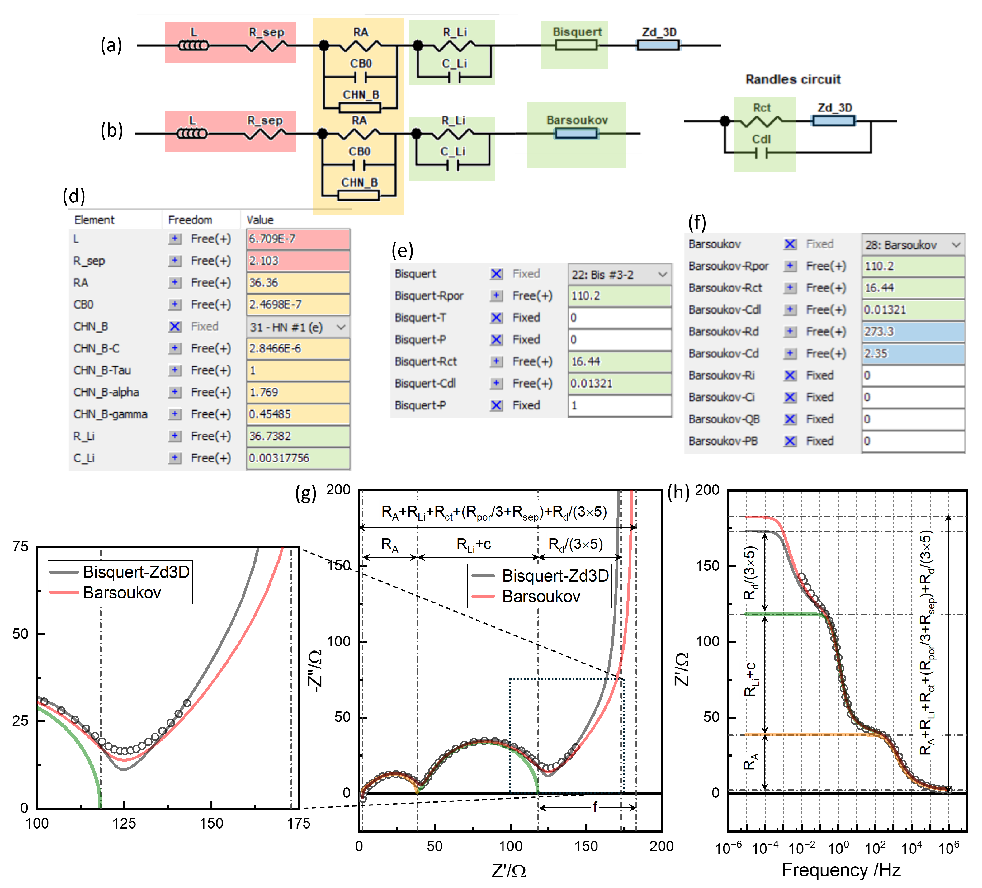
named as Barsoukov TLM in view of the extensive description[30]. The related battery models are available in MEISP[33] (or FitmyEIS[34]), or ZView® DX-28, can be used, as shown in Figure 11(b) and (f). As the relaxation times for are substantially longer, high-frequency response of can be described by
with =0 in Eq. 12, a model for electrodes in fuel cells or electrolyzers [35], which is known as a Bisquert TLM in view of the extensive work by Prof. Bisquert e.g.[36]. ZView® DX-22 model can be used as shown in Figure 11(a) and (e). The impedance magnitude of becomes
The c notation is after [3,4].
With substantial contribution to by the lithium counter electrode, separately confirmed [37] modeled as , is fitted (adjusted) to 110.2 and 16.44 , which gives c=43.05. With =36.74 becomes 79.78, as indicated in Figure 11 and Figure 12. The for NMC electrode is fitted to 0.01321 F and 0.003177 F, differ by the factor 4, but, as shown in the inset of Figure 11(c), the effects in EIS, affected by the series , are similar. The overall is somewhat reduced due to the series connection of the two capacitors and modified by R parameters. is now closer to the hump or minimum, reading position of than the conventional CPE fitting in Figure 9.
The substantial of the porous network in is indicated by the high-frequency slope-one behavior in the green spectrum, which is the overlapping range of and . The modeling is thus strongly correlated with the modeling of the response. The or is represented as a single , unlike two () modeling in the previous section. The additive capacitance functions describe the overlapped feature. A modified Debye circuit, or Havriliak-Negami capacitance,
with well-defined low-frequency limiting capacitance , and high-frequency limit . The exponents are fitted as =0.455 and =1.769, which is close to the versatile case of =0.5 and =2 [38,39,40]. The model is more excellent than the strongly overlapping ()s, since and and are directly indicated in the raw data, Figure 12(c). The distributed capacitance can physically describe the lateral inhomogeneity in the electrode and current collector interface. The well-defined limiting corresponds less depressed arc at the low frequency, shown in detail in the inset of Figure 12(a), compared to Figure 11(b). It is also shown that is closer to the intercept than for the conventional CPE fitting with =0.57≪1, Figure 9.
The capacitance function, physically shown to block the electrolyte rail in Figure 10, can be directly connected in parallel to and can also be connected outside the TLM. The ohmic resistance of the separator, or is notated as , represented as n resistors of , which is trivial for =1, can also be connected outside the TLM. The black round boxed part can be thus represented by the model Figure 11(b).
Characteristic SOC dependence in or is due to charge transfer resistance of NMC electrode, [4,6,7]. and are likely to dullify the SOC dependence of in or . Ideal Bisquert TLM and parallel circuit describe the data excellently (correlated with the modeling of ) and R and C parameters are obtained without complications in using CPEs in the previous section, Figure 9. The results also indicate the poor reliability in the separated parameters, as the respective NMC electrode and Li electrode response are not ideally described [4,6,7,41]. Similarly, as CPE modeling, modeling of the multiple responses can describe the overall data with large correlated uncertainties in the parameters. For the theoretical discussion in the following, these parameters are used and =819.9, the adjusted one to the final model in Figure 12. in Figure 11 is defined as 819.9/3=273.3.
Figure 11(g,h) shows the difference when the diffusion impedance is properly included in TLM, notated as “Barouskov”, (b) in comparison when it is connected in series to the electrode reaction, notated as “Bisquert-Zd3D”, (a), often done in the literature, as pointed out in the previous section. while for “Bisquert-Zd3D”, , are simply added.
Diffusion impedance in TLM increases the DC limit resistance, , with non-negligible , on the other hand. The overall DC resistance of Barsoukov TLM, , of TLM, becomes
where , pore resistance , as for , Warburg Open, and for are simply added, as if they are connected in series. They do not match the well-distingished in EIS, which is , Eq. 14 and plus . The additional resistance due to the solid-state diffusion becomes
which becomes , only when =0. With non-negligible , i.e. for TLM, The c and f cannot be simply attributed to the single or components. The resistance values read from the plots or determined by the conventional modeling do not provide clear physical significance. The physics-based EIS modeling should deconvolute the meaningful R parameters.
As shown more clearly in the magnified view in Figure 12(b), the transient above for porous electrodes, the “Barsoukov” case, describes the raw data better in that the transition is more smoothly connected, compared to , Eq. 7, connected to the “Bisquert” response in series. parameter 819.9 could be better adjusted but is kept to the final adjustment for the liquid phase diffusion in the following section for clarity.
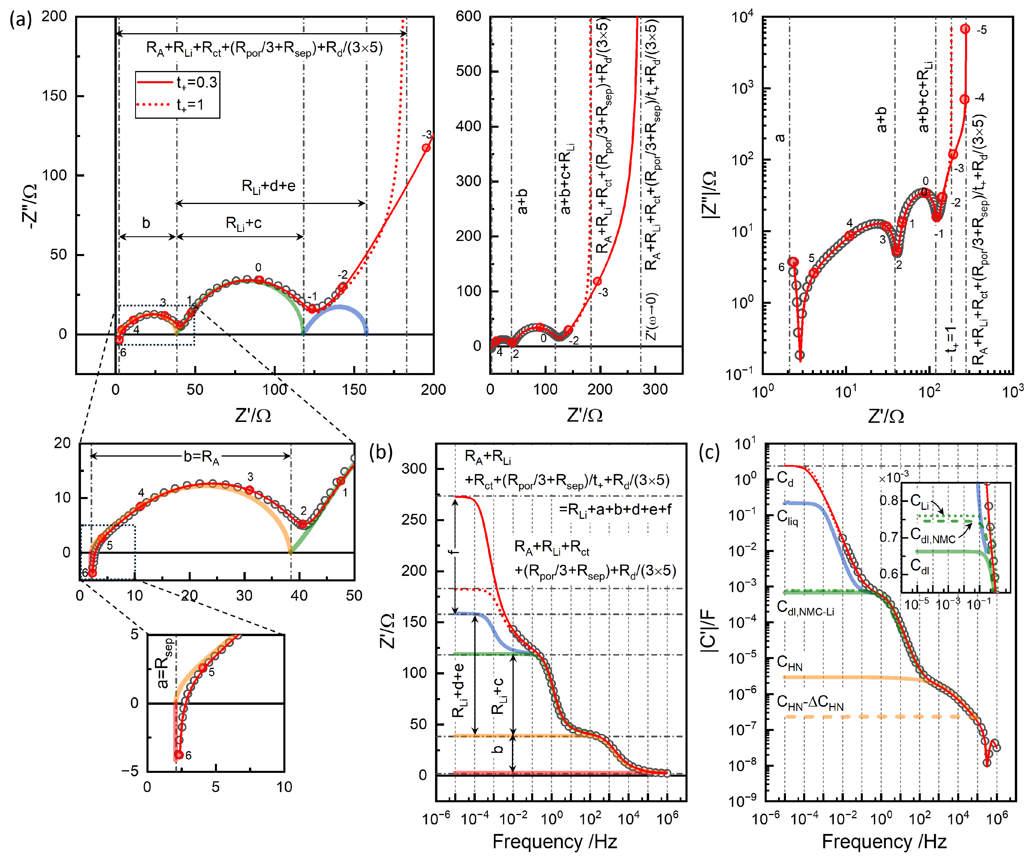
Figure 12.
3-rail TLM simulations for =1 and 0.3: (a) impedance plane plots in different ranges of linear and logarithmic scales; (b) Real impedance Bode plot; and (c) Capacitance Bode plot. Colored partial spectra indicate and and , , from raw data Figure 6(c,d,e).
Figure 12.
3-rail TLM simulations for =1 and 0.3: (a) impedance plane plots in different ranges of linear and logarithmic scales; (b) Real impedance Bode plot; and (c) Capacitance Bode plot. Colored partial spectra indicate and and , , from raw data Figure 6(c,d,e).
9. EIS vs. GITT: Transference Number
In the Barsoukov model discussed above, the electrolyte in the separator, , and in pores is considered a pure resistor. On the other hand, Newman’s battery model is centered on diffusion in the solution or electrolyte, which arises because negative ions, here, , unused, build up the salt concentration gradient, whereby the Li+ ion transport occurs, which is described by the solution diffusivity, [42]. The concentration gradient established in the liquid phase can be seen in battery simulations by Newman’s model, e.g., PyBaMM [43].
The impedance study according to Newman’s model [44,45,46] pointed out that the chemical diffusivity of active material cannot be correctly estimated since the solution diffusion process overlaps. Although liquid diffusivity, 10−6cm2s−1, is far higher than solid-state diffusivity, 10−11cm2s−1, as the effective diffusion length of the electrodes and the separator can be 3 to 5 times the nominal thickness 180m and 25m, due to the tortuosity, which is much larger than the active particle size 2.54m for solid-state diffusion. As the relaxation times increases with the squared distance over the diffusivity, they can be comparable [46].
In Newman’s concentrated solution theory for lithium-ion battery electrolytes the parameters of kinetic interactions between solvated cations, solvated anions, and large solvent molecules are involved in the diffusivity, , conductivity, , and transference number, . Most applications of the Newman model do not consider full kinetic parameters for interactions, but independently varied , conductivity, [44,45,46].
When Nernst-Planck flux behavior of the binary electrolyte, Li+ and , is assumed, ambipolar diffusion occurs similar to the for the lithium intercalation in the active mixed-conductor material, Eq. 4, as
where represents the liquid electrolyte conductivity. and the
which can be represented by the equivalent circuits in the lower blue box in Figure 10. The Nernst-Planck model of LIB appears roughly and self-consistently applicable since the determination by the Bruce-Vincent method [47], widely used, is also based on the Nernst-Planck model. Newman’s model becomes the Nernst-Planck model for the dilute solution as the kinetic interactions are negligible [42]. Nernst-Planck model is centered on the charge neutrality between the two carriers and the thermodynamic activity different from the ideal dilute solution can be still addressed in , similarly as for defined by the lithium activity represented by OCV [48].
Moškon et al.[3,4] practically simplified a more rigorous 3-dimensional network, as also reported by Siroma et al.[49], into the 2-dimensional 3-rail TLM in Figure 10, where the porous electrode model discussed above and the Nernst-Planck electrolyte model are combined. In the present version, the parameter is applied consistently to the liquid electrolyte in different regions, which is physically reasonable and simplifies parameter fitting (adjustment).
The porous battery electrode or the Barsoukov model considered in the previous section corresponds to the Li+ transference number =1. for LIB electrolytes by Bruce-Vincent method are around 0.3 [50]. The principle is more rigorously and practically applicable by measuring EIS down to the low frequency close to DC limit without DC polarization [37,51] and values around 0.3 are found for 1M LiPF6 EC:DMC 1:1 [37].
The full equivalent circuit in Figure 10 describes essential reactions in solids and liquids and interfaces in a physics-based way. A numerical calculation is required to describe the three-rail TLM and/or the liquid electrolyte TLM through different regions like the separator and electrodes [41]. The code was provided to J.S.L. by Prof. M. Gaberšček in 2023, June, and is now available in the supplementary information of Ref. [6,7].
The blue spectrum indicated in Figure 12, simulated with =0, represents the simulation of additional impedance when =0.3 compared to =1, Figure 11, involving the chemical capacitance and . The respective Li+ ion resistance are =2.103/0.3=7.01, and =109.9/0.3=366.3, and PF−6 ion resistance, =2.103/0.7=5.00, and =109.9/0.7=157.
The additional contribution in the blue spectrum from the separator with =0.3 is thus
amounting to 4.907. For pores in the electrode, replaces in Eq. 14
amounting to 77.72, whereas c = 43.05, and thus = 34.67 is the additional contribution. The magnitude of the additional impedance represented by the blue spectrum is thus =39.58.
The diffusional relaxation is represented by and as [52,53].
where and are effective length of the tortuous liquid paths. The factor becomes 4.76 for =0.3.
While it is likely that , as 4.907 vs. 34.67, and that , the two responses are not distinguished in the experimental data [4,6,7]. It is assumed =2.1 F from the capacitance value indicated in the raw data, Figure 6(f), , corresponds to of the chemical capacitance of the `Jamnik-Maier model’ [52,53]. The factor 3 for Warburg Short behavior and from the halved diffusion length in the symmetric cells. The model can be analyzed/simulated using ZView® DX-15, for example.
With these parameters determined and/or assumed so far, i.e., =2.35 F, from GITT OCV, , , , , , , from Bisquert model for porous electrodes, and with assumed, or separately determined, and = 2.1 F from the indication in the raw data in Figure 6(f), is best adjusted to 819.9, Figure 12, which is less than from GITT analysis, shot-time extended, 2054, highlighted in Figure 8(d), or 2174 from the equivalent EIS analysis, Figure 8(d), and the corresponding increase in , Figure 8(a), from the highlighted value. The difference is within a factor 3. The overall DC resistance can be generalized as
which becomes Eq. 16 for =1, Figure 12 and f indicated in Figure 12.
with d in Eq. 21 and e in Eq. 20.
Due to the difficulty in reliable estimation of the parameters in , i.e., in separating and with parameters and , the present analysis is limited to one data of Step 46 for a theoretical demonstration. When and are properly estimated from the symmetrical cells or half cells of three-electrodes cells, using the physics-based model, a stronger SOC dependence is likely observed. Dee et al. [2] reported a stronger OCV dependence of of an NCA electrode from Newman’s model compared to GITT analysis. A strong decrease in of an NCA electrode with OCV was found [37]. The strong OCV-dependent kinetics of NMC 622 electrode is also suggested by the relaxation behavior observed in this work, Figure 5.
10. Outlook
After more than a decade of efforts for GITT combined with EIS studies led by J.S.L, GITT is not considered a useful method for determining the chemical diffusivity of battery electrodes. Apart from the current status of too long pulse time and likely insufficient relaxation times, against the original principle and purpose for short-time diffusion solution and the equilibrium OCV curves, the response of the liquid phase in pores is likely to affect the GITT analysis for solid phase diffusivity strongly. Uncharacteristic OCV dependence of the diffusivity observed in many studies [11,12,13,14,15,16,17,18,19,20,22,23] suggested to be the indication of the liquid-phase diffusion.
Despite important physics-based insights into EIS, numerical or unwieldy analytic models [44,45,46,49] have been very limited in raw data analysis, since the experimental data must be compared with the simulation for each set of parameters to be adjusted. The Python code for the 3-rail TLM [6,7] is simple and the calculation is much faster than the rigorous network with negligible accuracy loss [4]. The 3-rail TLM by Gaberšček et al. has been demonstrated for experimental data [3,4,6,7,41]. The analysis can be rigorously applied to symmetric cells [6,7] or three-electrode cells [37], which are the single-electrode responses. For essential low-frequency information, e.g., down to 10−4 Hz within a practical time, ca. 3 h, multi-sine EIS can be utilized, available in commercial instruments [37].
As demonstrated in Figure 11, the Bisquert or Barsoukov TLM, or a general two-rail TLM has an analytic solution [54], and the parameters can be fitted using optimization algorithms. The liquid phase diffusion represented by , , and , and the solid-state diffusion, by and , overlap non-trivially, as indicated by d and f. The determination of these parameters or deconvolution of the two diffusion processes should be done by manual adjustment using 3-rail simulations, which seem to require insight, expertise, time, and patience [3,4,6,7,41]. Recently, an approximate two-rail TLM has been developed for the three-rail TLM[55], where Nernst-Planck liquid electrolyte TLM is approximated by simplified lumped circuits in the two-rail porous electrode model, so that optimization using analytic two-rail TLM is possible.
Even with such a substantial advance, as a general problem in the least-squares fitting for the multiparameter determination, the unphysical correlation of the fit parameters is difficult to avoid or control. EIS of the temperature-dependent multiple data set can address the unphysical correlation of the fit parameters in the single data analysis [31,51]. It has recently proved to be a powerful approach in battery EIS where temperature-independent C parameters and contact impedance can be uniquely separated from Arrhenius behavior R parameters when multiple data at different temperatures are fitted together [37]. Application to NMC622 and other electrode materials is under progress.
11. Conclusions
The current status of GITT for battery electrodes faces two major challenges that contradict its original principles and purpose: (1) the use of excessively long pulse times in short-time GITT analysis and (2) insufficient relaxation time, which prevents the system from reaching complete equilibrium. More critically, the method assumes a sequential reaction-diffusion process for thin-film electrodes, which is not applicable to active particles dispersed in porous electrodes, especially considering liquid-phase diffusion where = 0.3. The weak OCV dependence of chemical diffusivities in NMC622 and other layered oxides observed in GITT is likely due to overlapping liquid-phase diffusion in the transient response. In contrast, strong dependence in solid-state kinetics is evident in non-trivial relaxation behavior, such as the indefinite linear decay at high OCV. To accurately deconvolute liquid- and solid-phase diffusion, a physics-based 3-rail transmission line model (TLM) must be applied. Temperature-dependent EIS measurements across multiple cells at different SOC levels, combined with the development of an analytical approximation for the numerical 3-rail TLM, will pave the way for a breakthrough in the practical and powerful application of EIS in battery research.
Author Contributions
Conceptualization, J.S.L. and E.C.S.; methodology, J.S.L. and E.C.S.; software, T.L.P and S.H.; validation, J.S.L., H.H.C., and J.L.; formal analysis, A.I., T.L.P, and J.S.L.; investigation, A.I., T.T.T.N., T.T.T.H., N.A.G., P.C.W, S.B.Y., and O.J.L.; data curation, A.I. and J.S.L.; writing—original draft preparation, A.I., T.T.T.N.; writing—review and editing, J.S.L; supervision, J.S.L., C.J.P., and J.K.; funding acquisition, J.K. and J.S.L. All authors have read and agreed to the published version of the manuscript.
Funding
This work was supported by the National Research Foundation of Korea (NRF) grants funded by the Ministry of Science and ICT (MSIT) (grant no. NRF - 2018R1A5A1025224) and also partly supported by "Regional Innovation Strategy (RIS)" through the NRF funded by the Ministry of Education (MOE) (2021RIS-002).
Data Availability Statement
The raw data supporting the conclusions of this article will be made available by the authors on request.
Acknowledgments
We greatly appreciate Prof. Miran Gaberšček, National Institute of Chemistry, Ljubljana, Slovenia, for providing the Python code in 2023, June, and for critical and valuable discussions.
Conflicts of Interest
The authors declare no conflicts of interest.
References
- Weppner, W.; Huggins, R.A. Electrochemical Methods for Determining Kinetic Properties of Solids. Annu. Rev. Mater. Sci. 1978, 8, 269–311. [Google Scholar] [CrossRef]
- Dees, D.W.; Kawauchi, S.; Abraham, D.P.; Prakash, J. Analysis of the Galvanostatic Intermittent Titration Technique (GITT) as applied to a lithium-ion porous electrode. Journal of Power Sources 2009, 189, 263–268. [Google Scholar] [CrossRef]
- Moškon, J.; Gaberšček, M. Transmission line models for evaluation of impedance response of insertion battery electrodes and cells. J. Power Sources Adv. 2021, 7, 100047. [Google Scholar] [CrossRef]
- Moškon, J.; Žuntar, J.; Talian, S.D.; Dominko, R.; Gaberšček, M. A powerful transmission line model for analysis of impedance of insertion battery cells: a case study on the NMC-Li system. J. Electrochem. Soc. 2020, 167, 140539. [Google Scholar] [CrossRef]
- Gaberšček, M. Understanding Li-based battery materials via electrochemical impedance spectroscopy. Nat. Commun. 2021, 12, 6513. [Google Scholar] [CrossRef]
- Firm, M.; Moškon, J.; Kapun, G.; Talian, S.D.; Kamšek, A.R.; Štefančič, M.; Hočevar, S.; Dominko, R.; Gaberšček, M. Novel Methodology of General Scaling-Approach Normalization of Impedance Parameters of Insertion Battery Electrodes–Case Study on Ni-Rich NMC Cathode: Part I. Experimental and Preliminary Analysis. Journal of the electrochemical society 2024, 171, 120540. [Google Scholar] [CrossRef]
- Firm, M.; Moškon, J.; Kapun, G.; Talian, S.D.; Kamšek, A.R.; Štefančič, M.; Hočevar, S.; Dominko, R.; Gaberšček, M. Novel Methodology of General Scaling-Approach Normalization of Impedance Parameters of Insertion Battery Electrodes–Case Study on Ni-Rich NMC Cathode: Part II. Detailed Analysis Using a Transmission Line Model. Journal of the electrochemical society 2024, 171, 120543. [Google Scholar] [CrossRef]
- Kim, J.H.; Park, K.J.; Kim, S.J.; Yoon, C.S.; Sun, Y.K. A method of increasing the energy density of layered Ni-rich Li [Ni 1- 2x Co x Mn x] O 2 cathodes (x = 0.05, 0.1, 0.2). J. Mater. Chem. A 2019, 7, 2694–2701. [Google Scholar] [CrossRef]
- Chen, Y.; Song, S.; Zhang, X.; Liu, Y. The challenges, solutions and development of high energy Ni-rich NCM/NCA LiB cathode materials. J. Phys.: Conf. Ser. 2019, 1347, 012012. [Google Scholar] [CrossRef]
- Noh, H.J.; Youn, S.; Yoon, C.S.; Sun, Y.K. Comparison of the Structural and Electrochemical Properties of Layered Li[NixCoyMnz]O2 (x = 1/3, 0.5, 0.6, 0.7, 0.8 and 0.85) Cathode Material for Lithium-Ion Batteries. J. Power Sources 2013, 233, 121–130. [Google Scholar] [CrossRef]
- Hyun, H.; Jeong, K.; Hong, H.; Seo, S.; Koo, B.; Lee, D.; Choi, S.; Jo, S.; Jung, K.; Cho, H.H.; et al. Suppressing High-Current-Induced Phase Separation in Ni-Rich Layered Oxides by Electrochemically Manipulating Dynamic Lithium Distribution. Adv. Mater. 2021, 33, 2105337. [Google Scholar] [CrossRef] [PubMed]
- Park, J.H.; Yoon, H.; Cho, Y.; Yoo, C.Y. Investigation of Lithium Ion Diffusion of Graphite Anode by the Galvanostatic Intermittent Titration Technique. Materials 2021, 14, 4683. [Google Scholar] [CrossRef] [PubMed]
- Li, Z.; Du, F.; Bie, X.; Zhang, D.; Cai, Y.; Cui, X.; Wang, C.; Chen, G.; Wei, Y. Electrochemical Kinetics of the Li[Li0.23Co0.3Mn0.47]O2 Cathode Material Studied by GITT and EIS. J. Phys. Chem. C 2010, 114, 22751–22757. [Google Scholar] [CrossRef]
- Verma, A.; Smith, K.; Santhanagopalan, S.; Abraham, D.; Yao, K.P.; Mukherjee, P.P. Galvanostatic Intermittent Titration and Performance-Based Analysis of LiNi0.5Co0.2Mn0.3O2 Cathode. J. Electrochem. Soc. 2017, 164, A3380. [Google Scholar] [CrossRef]
- Kim, J.; Park, S.; Hwang, S.; Yoon, W.S. Principles and Applications of Galvanostatic Intermittent Titration Technique for Lithium-Ion Batteries. J. Electrochem. Sci. Technol. 2022, 13, 19–31. [Google Scholar] [CrossRef]
- Juston, M.; Damay, N.; Forgez, C. Extracting the Diffusion Resistance and Dynamic of a Battery Using Pulse Tests. J. Energy Storage 2023, 57, 106199. [Google Scholar] [CrossRef]
- Shen, Z.; Cao, L.; Rahn, C.D.; Wang, C.Y. Least Squares Galvanostatic Intermittent Titration Technique (LS-GITT) for Accurate Solid Phase Diffusivity Measurement. J. Electrochem. Soc. 2013, 160, A1842. [Google Scholar] [CrossRef]
- He, L.P.; Li, K.; Zhang, Y.; Liu, J. Structural and Electrochemical Properties of Low-Cobalt-Content LiNi0.6+xCo0.2-xMn0.2O2(0.0≤x≤0.1) Cathodes for Lithium-Ion Batteries. ACS Appl. Mater. Interfaces 2020, 12, 28253–28263. [Google Scholar] [CrossRef]
- Wang, J.; Hyun, H.; Seo, S.; Jeong, K.; Han, J.; Jo, S.; Kim, H.; Koo, B.; Eum, D.; Kim, J.; et al. A Kinetic Indicator of Ultrafast Nickel-Rich Layered Oxide Cathodes. ACS Energy Lett. 2023, 8, 2986–2995. [Google Scholar] [CrossRef]
- Kang, S.D.; Kuo, J.J.; Kapate, N.; Hong, J.; Park, J.; Chueh, W.C. Galvanostatic Intermittent Titration Technique Reinvented: Part II. Experiments. J. Electrochem. Soc. 2021, 168, 120503. [Google Scholar] [CrossRef]
- Jetybayeva, A.; Schön, N.; Oh, J.; Kim, J.; Kim, H.; Park, G.; Lee, Y.G.; Eichel, R.A.; Kleiner, K.; Hausen, F.; et al. Unraveling the state of charge-dependent electronic and ionic structure–property relationships in NCM622 cells by multiscale characterization. ACS Appl. Energy Mater. 2022, 5, 1731–1742. [Google Scholar] [CrossRef]
- Cui, Z.; Guo, X.; Li, H. Equilibrium Voltage and Overpotential Variation of Nonaqueous Li-O2 Batteries Using Galvanostatic Intermittent Titration Technique. Energy Environ. Sci. 2015, 8, 182–187. [Google Scholar] [CrossRef]
- Assat, G.; Delacourt, C.; Dalla Corte, D.A.; Tarascon, J.M. Practical assessment of anionic redox in Li-rich layered oxide cathodes: a mixed blessing for high energy Li-ion batteries. J. Electrochem. Soc. 2016, 163, A2965. [Google Scholar] [CrossRef]
- Li, A.; Pelissier, S.; Venet, P.; Gyan, P. Fast Characterization Method for Modeling Battery Relaxation Voltage. Batteries 2016, 2, 7. [Google Scholar] [CrossRef]
- Ménétrier, M.; Carlier, D.; Blangero, M.; Delmas, C. On “Really” Stoichiometric LiCoO2. Electrochem. Solid-State Lett. 2008, 11, A179. [Google Scholar] [CrossRef]
- Kang, S.D.; Chueh, W.C. Galvanostatic Intermittent Titration Technique Reinvented: Part I. A Critical Review. J. Electrochem. Soc. 2021, 168, 120504. [Google Scholar] [CrossRef]
- Crank, J. The Mathematics of Diffusion; Oxford University Press, 1979. [Google Scholar]
- Kim, Y.H.; Shin, E.C.; Kim, S.J.; Park, C.N.; Kim, J.; Lee, J.S. Chemical Diffusivity for Hydrogen Storage: Pneumatochemical Intermittent Titration Technique. J. Phys. Chem. C 2013, 117, 19771–19785. [Google Scholar] [CrossRef]
- Shaju, K.M.; Rao, G.V.S.; Chowdari, B.V.R. EIS and GITT Studies on Oxide Cathodes, O2-Li2/3+x(Co0.15Mn0.85)O2 (x = 0 and 1/3). Electrochim. Acta 2003, 48, 2691–2703. [Google Scholar] [CrossRef]
- Barsoukov, E.; Macdonald, J.R. Impedance Spectroscopy: Theory, Experiment, and Applications; John Wiley & Sons, 2018. [Google Scholar]
- Linh, P.T. Python-assisted determination of kinetic parameters in oxygen-ion conducting ceramic membranes and Li-ion batteries. PhD thesis, Chonnam National University, 2021.
- Ansah, S.; Hyun, H.; Shin, N.; Lee, J.S.; Lim, J.; Cho, H.H. A Modeling Approach to Study the Performance of Ni-Rich Layered Oxide Cathode for Lithium-Ion Battery. Comput. Mater. Sci. 2021, 196, 110559. [Google Scholar] [CrossRef]
- Co., K.K.P. Co., K.K.P. MEISP 3.0: Multiple Electrochemical Impedance Spectra Parameterization. http://impedance0.tripod.com/##3, 2002.
- Chukwu, R. FitMyEIS - Electrochemical Impedance Spectroscopy Fitting Tool, 2025. Accessed: 2025-01-31.
- Shin, E.C.; Ma, J.; Ahn, P.A.; Seo, H.H.; Nguyen, D.T.; Lee, J.S. Deconvolution of four transmission-line-model impedances in Ni-YSZ/YSZ/LSM solid oxide cells and mechanistic insights. Electrochim. Acta 2016, 188, 240–253. [Google Scholar] [CrossRef]
- Bisquert, J. Influence of the boundaries in the impedance of porous film electrodes. Physical Chemistry Chemical Physics 2000, 2, 4185–4192. [Google Scholar] [CrossRef]
- Park, C.W. Enhanced Battery Characterization Using Physics-Based Models for State-of-Charge and Temperature EIS with a Three-Electrode System. PhD thesis, Chonnam National University, 2025.
- Abbas, A.; Jung, W.G.; Moon, W.J.; Uwiragiye, E.; Pham, T.L.; Lee, J.S.; Fisher, J.G.; Ge, W.; Naqvi, F.U.H.; Ko, J.H. Growth of (1- x)(Na1/2Bi1/2) TiO3–x KNbO3 single crystals by the self-flux method and their characterisation. Journal of the Korean Ceramic Society 2024, 61, 342–365. [Google Scholar] [CrossRef]
- Lee, K.; Yoon, D.; Kim, H.; Park, H.W.; Min, D.R.; Nguyen, D.T.; Shin, E.C.; Lee, J.S. TiO2 nanocone photoanodes by Ar ion-beam etching and physics-based electrochemical impedance spectroscopy. Electrochim. Acta 2024, 481, 143976. [Google Scholar] [CrossRef]
- Moon, S.H.; Kim, Y.H.; Cho, D.C.; Shin, E.C.; Lee, D.; Im, W.B.; Lee, J.S. Sodium ion transport in polymorphic scandium NASICON analog Na3Sc2 (PO4) 3 with new dielectric spectroscopy approach for current-constriction effects. Solid State Ionics 2016, 289, 55–71. [Google Scholar] [CrossRef]
- Drvarič Talian, S.; Bobnar, J.; Sinigoj, A.R.; Humar, I.; Gaberšček, M. Transmission line model for description of the impedance response of Li electrodes with dendritic growth. The Journal of Physical Chemistry C 2019, 123, 27997–28007. [Google Scholar] [CrossRef]
- Newman, J.; Balsara, N.P. Electrochemical systems; John Wiley & Sons, 2021. [Google Scholar]
- Sulzer, V.; Marquis, S.G.; Timms, R.; Robinson, M.; Chapman, S.J. Python battery mathematical modelling (PyBaMM). Journal of Open Research Software 2021, 9. [Google Scholar] [CrossRef]
- Doyle, M.; Meyers, J.P.; Newman, J. Computer simulations of the impedance response of lithium rechargeable batteries. Journal of the Electrochemical Society 2000, 147, 99. [Google Scholar] [CrossRef]
- Sikha, G.; White, R.E. Analytical expression for the impedance response of an insertion electrode cell. Journal of The Electrochemical Society 2006, 154, A43. [Google Scholar] [CrossRef]
- Huang, J.; Zhang, J. Theory of impedance response of porous electrodes: simplifications, inhomogeneities, non-stationarities and applications. J. Electrochem. Soc. 2016, 163, A1983. [Google Scholar] [CrossRef]
- Bruce, P.G.; Evans, J.; Vincent, C.A. Conductivity and transference number measurements on polymer electrolytes. Solid State Ionics 1988, 28, 918–922. [Google Scholar] [CrossRef]
- Jamnik, J.; Maier, J.; Pejovnik, S. A powerful electrical network model for the impedance of mixed conductors. Electrochimica Acta 1999, 44, 4139–4145. [Google Scholar] [CrossRef]
- Siroma, Z.; Fujiwara, N.; Yamazaki, S.i.; Asahi, M.; Nagai, T.; Ioroi, T. Multi-rail transmission-line model as an equivalent circuit for electrochemical impedance of a porous electrode. Journal of Electroanalytical Chemistry 2020, 878, 114622. [Google Scholar] [CrossRef]
- Zugmann, S.; Fleischmann, M.; Amereller, M.; Gschwind, R.M.; Wiemhöfer, H.D.; Gores, H.J. Measurement of transference numbers for lithium ion electrolytes via four different methods, a comparative study. Electrochimica Acta 2011, 56, 3926–3933. [Google Scholar] [CrossRef]
- Tran, T.H.T. Physics-based impedance modeling of mixed ionic electronic conductors, liquid/polymer/solid electrolytes, and human body segments. PhD thesis, Chonnam National University, 2024.
- Jamnik, J.; Maier, J. Treatment of the impedance of mixed conductors equivalent circuit model and explicit approximate solutions. J. Electrochem. Soc. 1999, 146, 4183. [Google Scholar] [CrossRef]
- Lee, J.S.; Jamnik, J.; Maier, J. Generalized equivalent circuits for mixed conductors: silver sulfide as a model system. Monatsh. Chem. 2009, 140, 1113–1119. [Google Scholar] [CrossRef]
- Adamič, M.; Talian, S.D.; Sinigoj, A.R.; Humar, I.; Moškon, J.; Gaberšček, M. A transmission line model of electrochemical cell’s impedance: case study on a Li-S system. Journal of the Electrochemical Society 2018, 166, A5045. [Google Scholar] [CrossRef]
- Shin, E.C.; Ryu, J.H.; Ka, B.H.; Lee, J.S.; Jeong, D.H.; Ho, K. Method and apparatus for lithium ion battery impedance analysis. 10-2025-0001795, 2025.
Figure 1.
(a) The first 10 charge/discharge cycles of a NMC622 half coin cell. (b) Differential capacity curves. (c) Charge/discharge potential and temperature vs. time.
Figure 1.
(a) The first 10 charge/discharge cycles of a NMC622 half coin cell. (b) Differential capacity curves. (c) Charge/discharge potential and temperature vs. time.
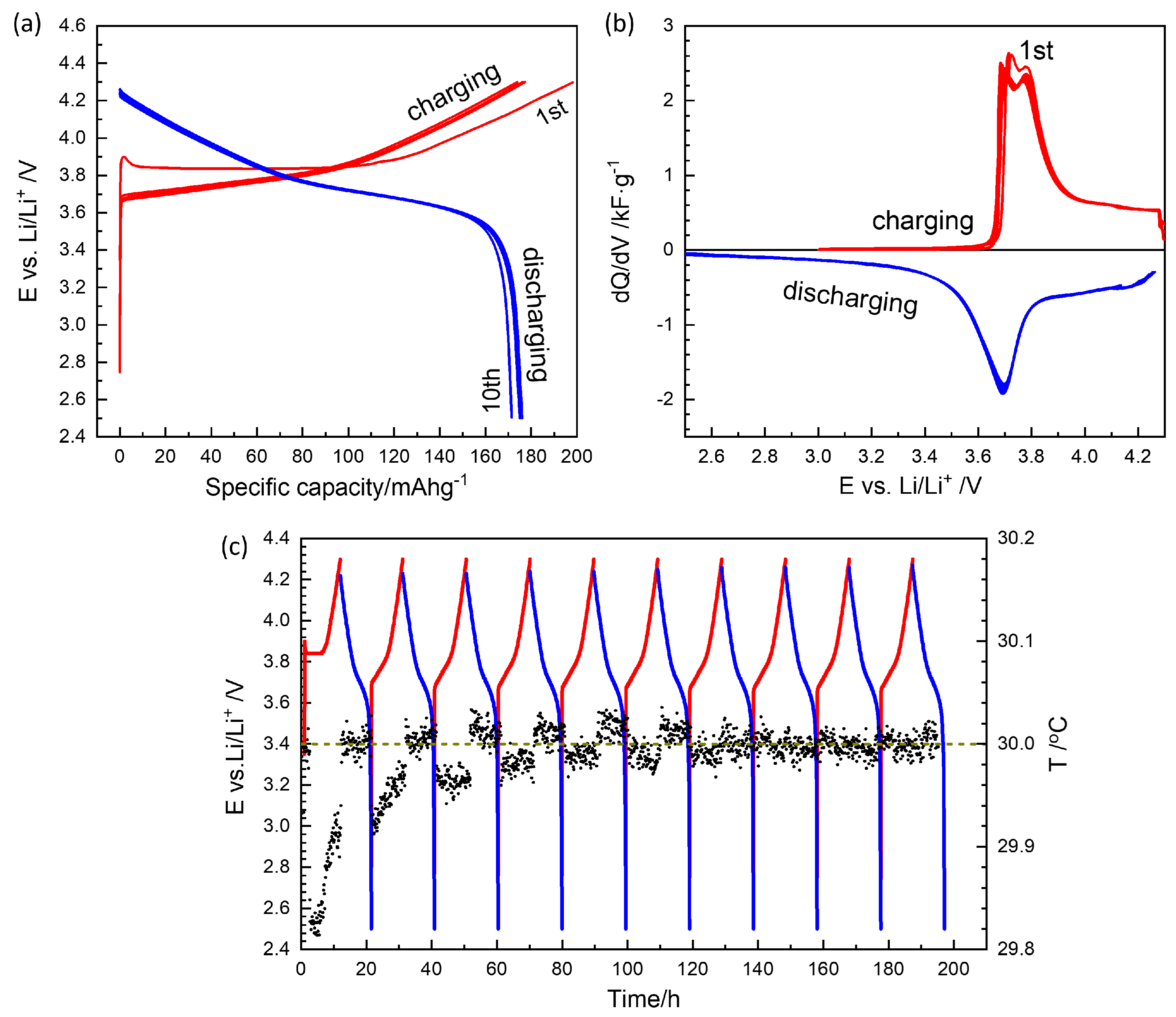
Figure 2.
Potentials during GITT as a function of time (left) and capacity (right). The symbols indicate equilibrium OCV points. Steps 2 and 60 are for Figure 3, 61 and 111 for Figure 4. Step 46 is the example data of the main analysis and discussion.
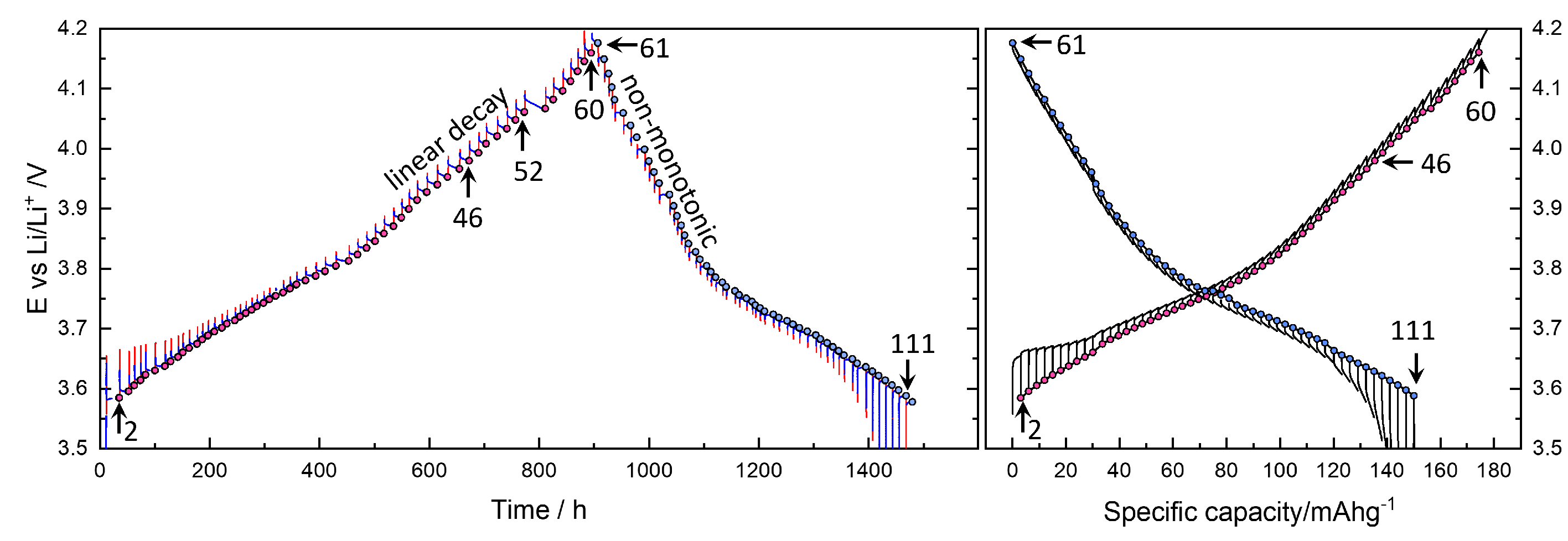
Figure 3.
Relaxation at charging Step 2 and Step 60 (a,d), (b,e) and (c,f).
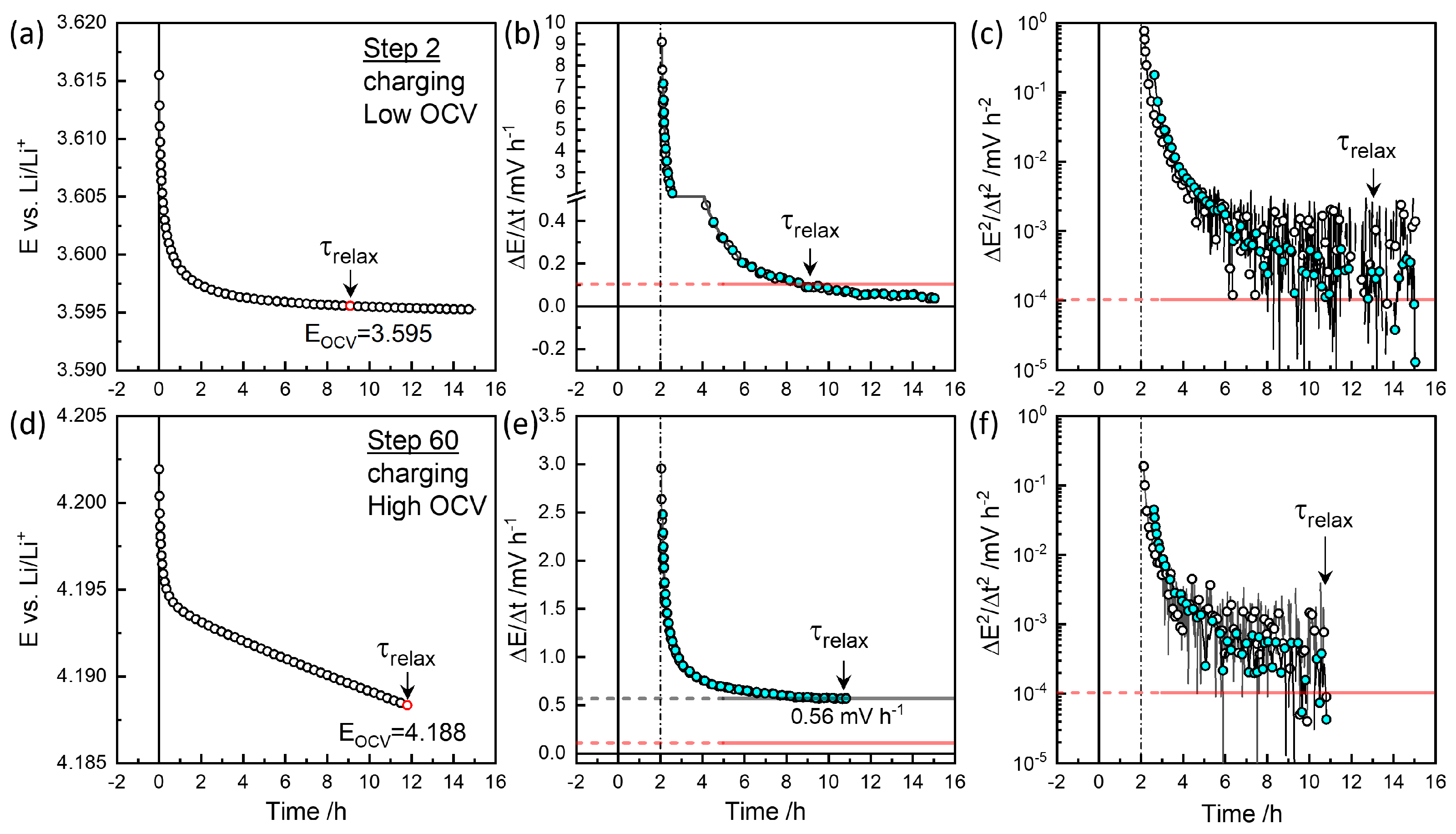
Figure 4.
Relaxation at discharging Step 61 and Step 111 (a,d), (b,e) and (c,f).
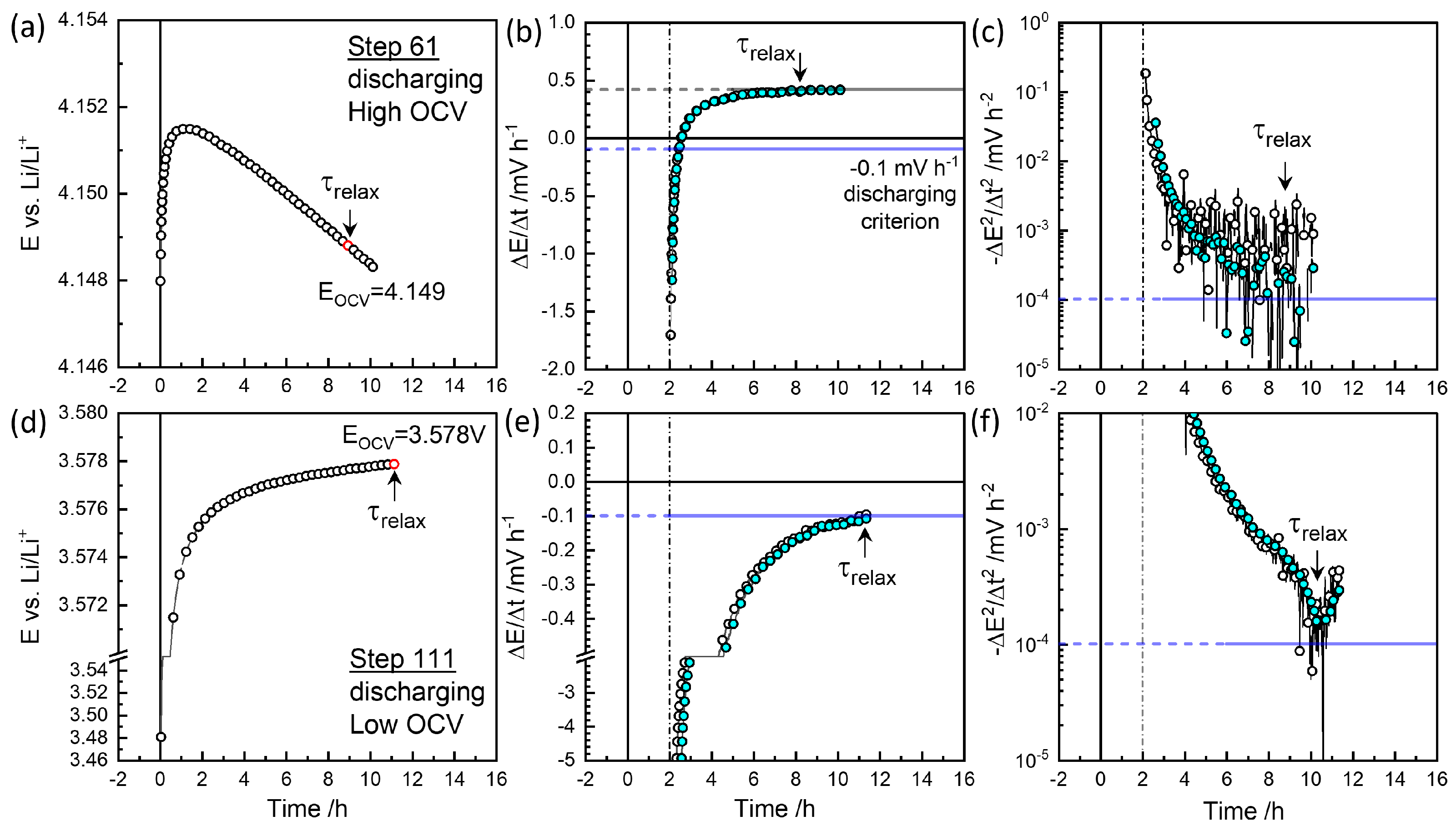
Figure 5.
Relaxation times at = 0.1 mV h−1 (in squares) below 3.8 V or = 10−4 mV h−2 with values increasing up to 0.56 mV h−1 above ca. 3.8 V (in circles) upon charging (a) and discharging (b). For the normal discharging in the opposite direction, = - 0.1 mV h−1. Peculiar non-monotonic relaxations observed at high OCV are indicated by the positive as on charging.
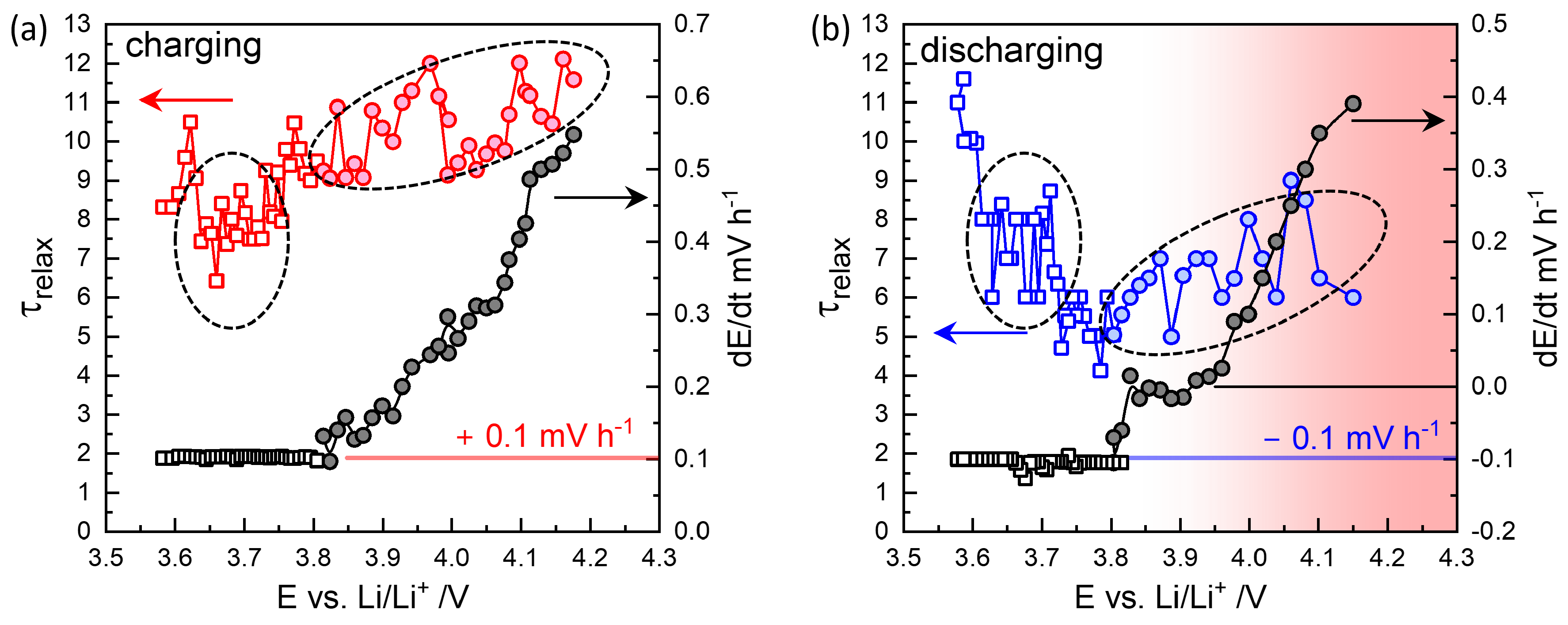
Figure 6.
(a) Polarization and relaxation at charging Step 46 with from and indicated. Corresponding resistance using are indicated on the right axis. (b) Log-log plots for the short-time behavior. (c) vs for GITT analysis. (d) Impedance measured at OCV=3.966 V before titration in (a). Graphically distinguishable resistance points, , , and are indicated. Note that they are not segmental values. (e) The real impedance Bode plot in the logarithmic scale with the resistance points in (d) indicated, and contribution from GITT analysis. (f) Capacitance Bode plot of the raw data (black), and those with , , and subtracted, respectively, directly providing capacitance values associated with the respective impedance arcs.
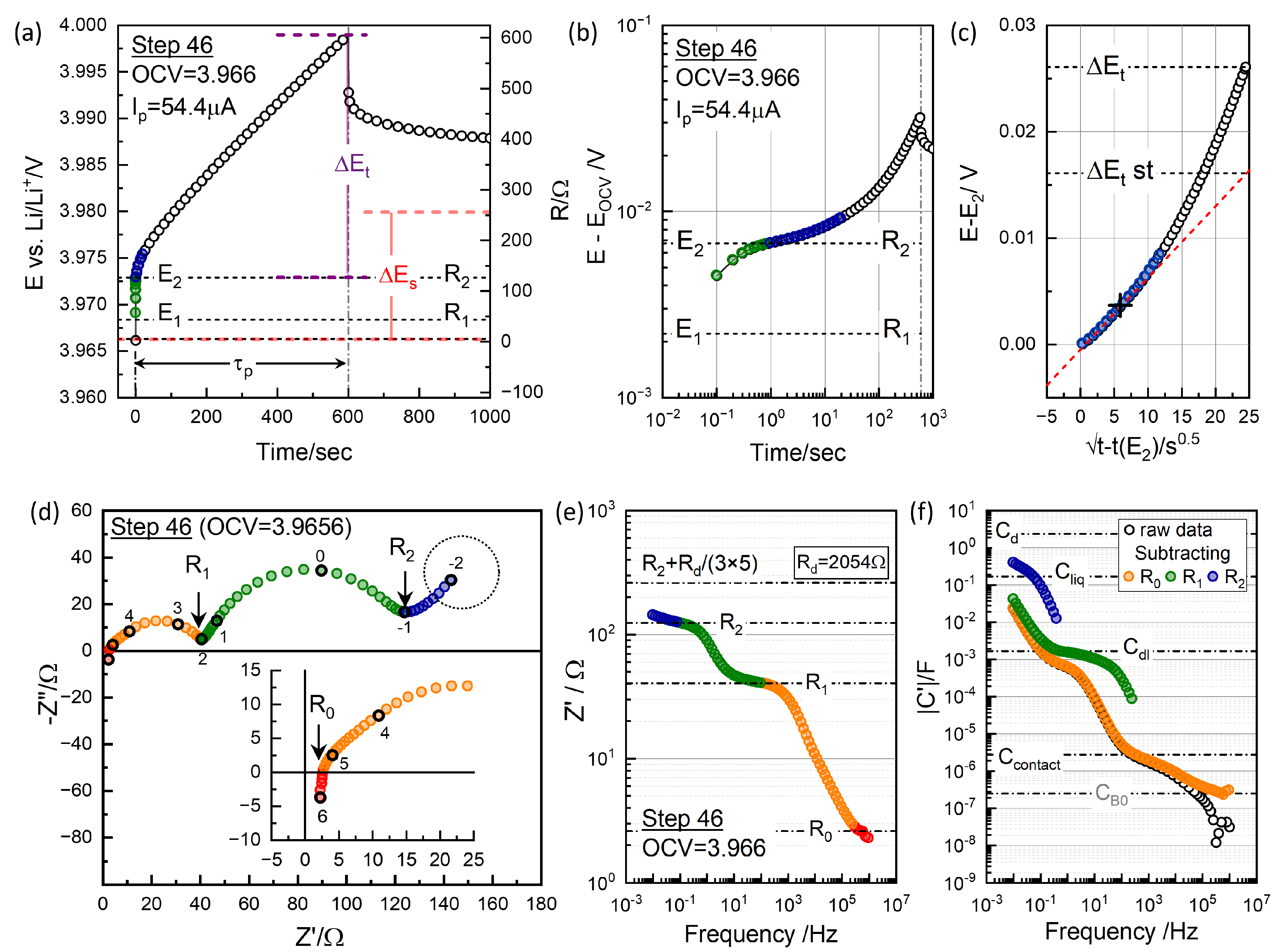
Figure 7.
Selected impedance spectra from charging steps (a) and discharging steps (b) with R parameters as a function of OCV distinguished in the impedance spectra, , , and .
Figure 7.
Selected impedance spectra from charging steps (a) and discharging steps (b) with R parameters as a function of OCV distinguished in the impedance spectra, , , and .
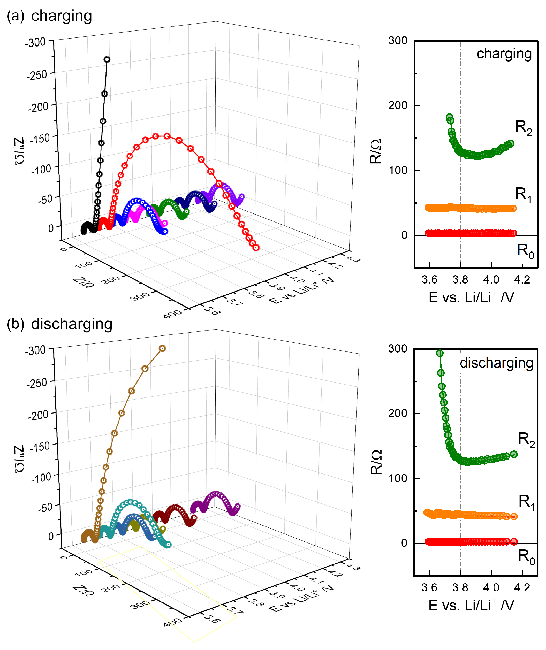
Figure 8.
(a) from charging and discharging GITT analysis. (b) and for charging and discharging steps. (c) and (d) as a function of OCV. The highlighted symbols for Step 46 in Figure 6 and the evaluation using EIS in Figure 12.
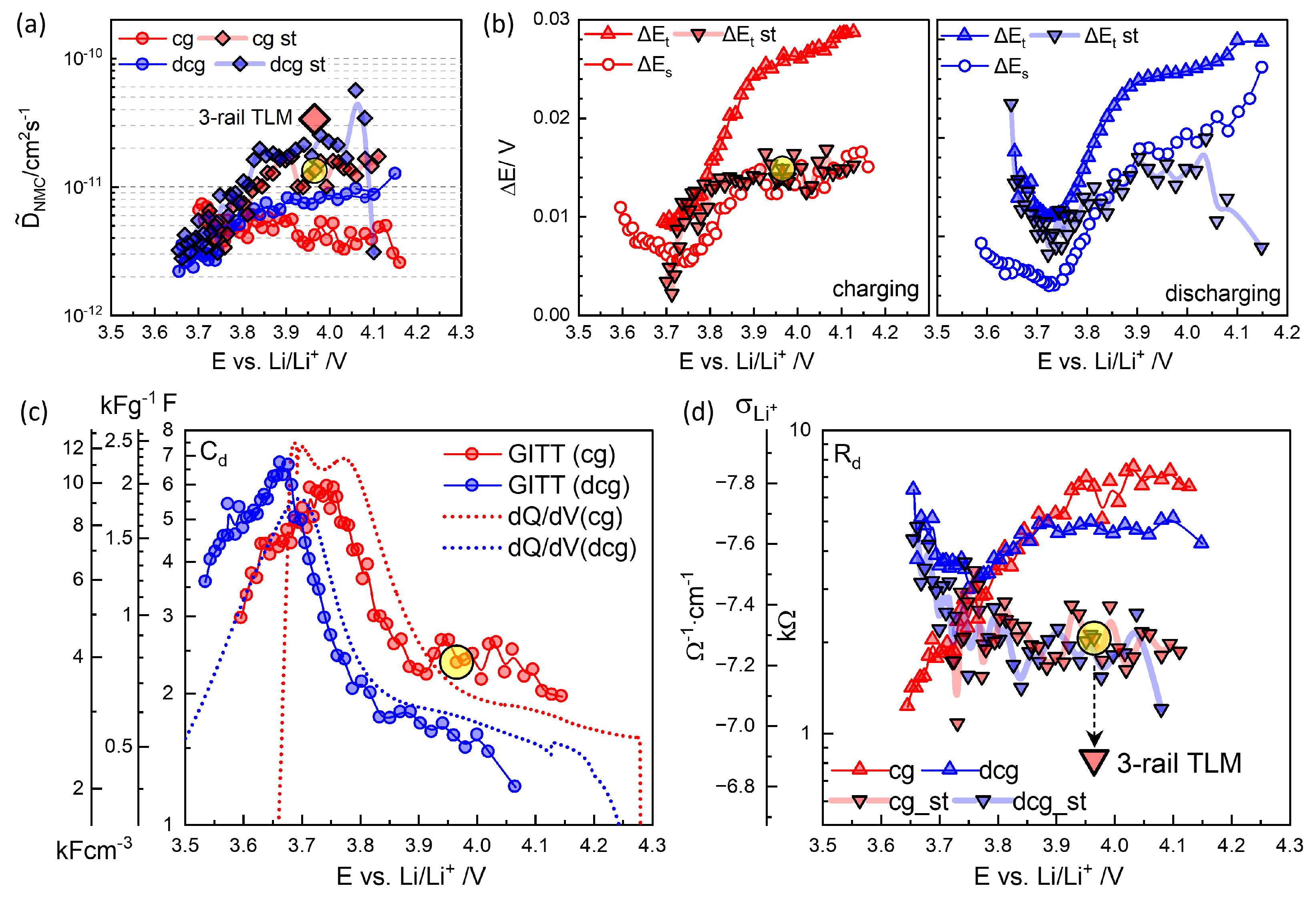
Figure 9.
(a)(b)(c) Impedance data of Step 46 (in circles) and fitted results (in crosses) to the equivalent circuit (d) or (e). Partial spectra simulated using the models corresponding to , , are indicated in colors. Havriliak-Negami impedance function (e) is equivalent but superior to conventional CPE modeling (d), since values are directly parameterized.
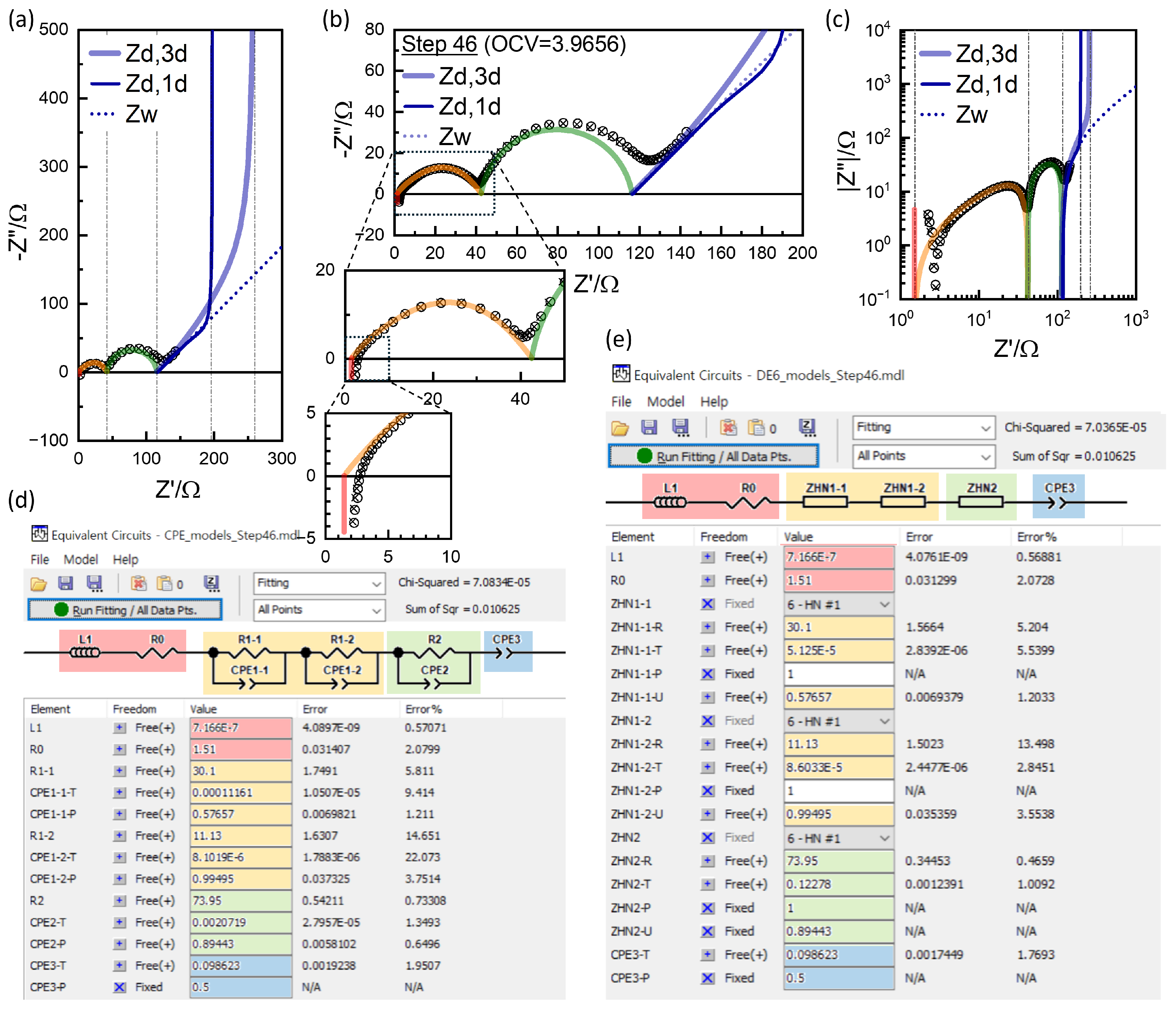
Figure 10.
3-rail-TLM NMC-Li cell (adapted from [4] and the parameters for the simulations in Figure 12.
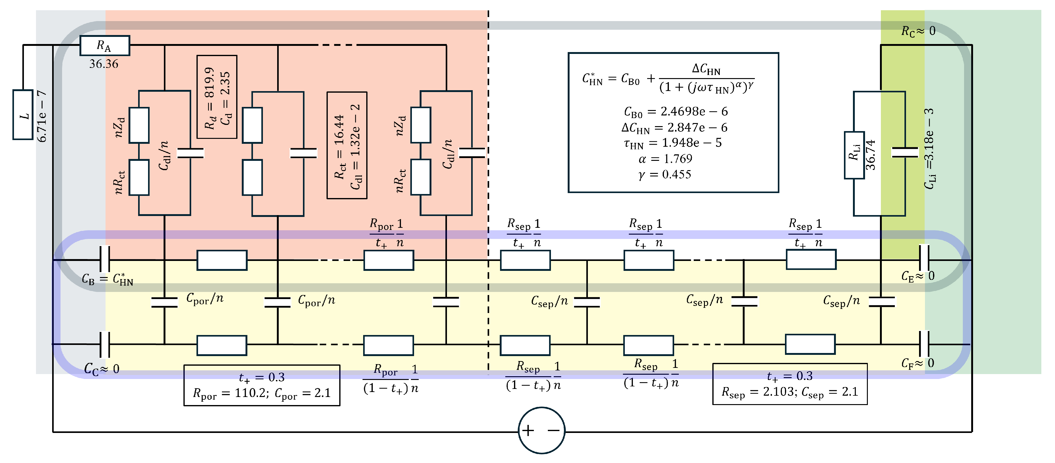
Figure 11.
(a) Bisquert TLM (ZView® DX-22) for porous electrodes with the distributed , , and parameters in (d) and the diffusion impedance connected in series as in Figure 9. (b) Barsoukov TLM (ZView® DX-28) with the parameters in (e) where the diffusion impedance is also distributed together with and in Randles circuit as in Figure 10. Bisquert TLM and are for the response. Contact impedance is described as (=) in parallel with a Havriliak-Negami capacitance (ZView® DE-31) with the parameters in (c). Impedance plane plots (f) and Bode plots (g) for the two equivalent circuits.
Disclaimer/Publisher’s Note: The statements, opinions and data contained in all publications are solely those of the individual author(s) and contributor(s) and not of MDPI and/or the editor(s). MDPI and/or the editor(s) disclaim responsibility for any injury to people or property resulting from any ideas, methods, instructions or products referred to in the content. |
© 2025 by the authors. Licensee MDPI, Basel, Switzerland. This article is an open access article distributed under the terms and conditions of the Creative Commons Attribution (CC BY) license (http://creativecommons.org/licenses/by/4.0/).
Copyright: This open access article is published under a Creative Commons CC BY 4.0 license, which permit the free download, distribution, and reuse, provided that the author and preprint are cited in any reuse.


