
Submitted:
22 August 2025
Posted:
27 August 2025
You are already at the latest version
Abstract
Ice accretion (icing) on aircraft surfaces is a significant safety risk through airfoil shape modification and reduction of aerodynamic efficiency. This process occurs when an aircraft flies through clouds of supercooled water droplets that freeze upon impact on exposed surfaces. To counter this hazard, electro-thermal de-icing systems integrate heaters in critical regions to melt ice and reduce performance losses. In this study, a multiphysics computational model is used to simulate ice accretion and electro-thermal de-icing on a NACA-0012 airfoil, accounting for factors such as airflow, droplet impingement, phase changes, and heat conduction. The model's predictions are validated against experimental data, confirming its accuracy. A cyclic electro-thermal ice protection system (ETIPS) is then tested under both standard and severe supercooled large droplet (SLD) conditions, examining how droplet size and angle of attack affect de-icing performance. Simulations without an active de-icing system show severe aerodynamic degradation, including an 11.1% loss of lift and a 48.2% increase in drag at a 12°∘ angle of attack. For large droplets (median 200 μm ), the drag coefficient increases by 36.5%. Under harsh icing conditions, the effectiveness of the de-icing system is found to depend on droplet size, angle of attack, and heater placement. Even with continuous heater operation, ice continues to accumulate on the leading edge at higher angles of attack. While the ETIPS performs effectively against large droplets in its protected zones, unheated regions experience significant ice buildup (especially with 200 μm droplets), indicating that additional or extended heaters may be necessary to ensure complete protection in extreme conditions.
Keywords:
ice accretion
; electro-thermal de-icing
; conjugated heat transfer
; supercooled large droplets
1. Introduction
Aircraft icing is a significant issue in aviation where an aircraft flies through a cloud of supercooled water droplets that freeze upon impact with its surfaces [1,2,3,4]. The most vulnerable areas prone to icing are wing leading edges, engine inlets, and windshield windows since these parts are directly exposed to incoming airflow and droplet impacts. Ice accumulation changes aerodynamic profiles, reducing performance, adding drag, and affecting stability and control [5,6,7]. Moreover, crushed ice fragments may damage internal components or enter the engine, reducing thrust or blocking the inlets [8,9]. Understanding when and how icing forms determines the variables that control its severity.
Several environmental and operational variables influence the extent of ice accretion. Airspeed, temperature, droplet size, liquid water content (LWC), and exposure time are some of the variables that affect the quantity of ice accretion under icing circumstances [10].The primary ice types are rime, glaze, and mixed: rime forms when small supercooled droplets freeze on impact at low temperature and low LWC, producing a rough, opaque, porous deposit; glaze forms when larger droplets and higher LWC near 0° allow water to spread and refreeze, yielding dense, transparent layers with runback horns; and mixed ice exhibits characteristics of both and can severely degrade aerodynamic performance [10,11,12]. Within this spectrum, one regime–Supercooled Large Droplet (SLD) icing–demands particular attention due to its operational risk.
SLD icing gained heightened attention in the aerospace industry after the fatal 1994 ATR-72 crash, which was attributed to ice buildup on the aircraft’s trailing-edge flaps leading to loss of control. This accident underscored the importance of understanding in-flight SLD icing and its effects on the aerodynamic performance of high-lift configurations. In response, research efforts have intensified to better understand SLD icing phenomena and associated hazards [13,14]. These risks, in turn, motivate robust and energy-efficient ice protection strategies on modern aircraft.
Commercial aircraft employ various Ice Protection System (IPS) technologies to prevent or remove ice. The most commonly used systems include engine bleed-air heating, electro-thermal heaters, pneumatic de-icing boots, and weeping wing (fluid) systems. Among these, hot-air and electro-thermal ice protection systems (ETIPS) are especially prevalent, with ETIPS gaining popularity due to their higher energy efficiency [15,16]. ETIPS are favored in modern aircraft designs because of their relative simplicity and energy efficiency [16], offering power savings of up to 33% compared to traditional thermo-pneumatic systems [17]. However, selecting how and where to apply heat introduces fundamental trade-offs between continuous prevention and periodic removal. IPS design strategies typically combine anti-icing and de-icing methods depending on aircraft requirements: some critical surfaces are continuously heated (anti-icing) while others allow ice to accumulate briefly before periodic removal (de-icing) [18]. A key trade-off exists between these approaches: anti-icing systems prevent ice from forming but consume more energy, whereas de-icing systems allow a thin ice layer to form and then shed it, using less energy overall [19,20]. Consequently, ETIPS are often designed to maximize efficiency by operating in a de-icing mode, which has been shown to be more energy-efficient than continuous anti-icing [21,22]. Furthermore, hybrid approaches that combine passive and active techniques (e.g., superhydrophobic coatings with electro-thermal heating) have proven effective in lowering energy consumption [23,24]. Because these design choices carry safety and energy implications, rigorous assessment methods are essential.
Developing and certifying an IPS can be costly, time-consuming, and even dangerous—especially if flight tests in natural icing conditions are required. Consequently, there is growing interest in Certification by Analysis (CbA), wherein numerical simulations supplement or replace some physical icing tests [25]. Accurate computational models are essential for designing efficient aircraft IPS. These simulations must capture complex phenomena including aerodynamic flow, droplet impingement, phase transitions (freezing and melting), heat transfer, and water film runback behavior [7,26,27,28]. This need has driven a mature ecosystem of icing simulation tools.
Several icing codes have been developed to estimate ice accretion on complex geometries. Representative examples include ANSYS FENSAP-ICE (commercial), NASA’s LEWICE (2D/3D; government-distributed), ONERA’s 2D/3D icing modules, and research/industry tools such as ICECREMO, CANICE, and PoliICE [7,29,30]. Other institution-specific frameworks—including the NRC Morphogenetic Code, IGLOO3D, PoliMIce, SIMBA/MESS3D, and ONICE3D—are not generally available to the public [31]. Availability and licensing therefore vary (commercial, government-distributed, or restricted), and most packages are not openly released or open-source. These tools typically employ Reynolds–Averaged Navier–Stokes (RANS) solvers, with the one-equation Spalart–Allmaras model commonly used for boundary-layer flows where icing originates [32]. Furthermore, time-resolved ice-shape evolution can be captured via multi-shot approaches combined with automatic remeshing, improving predictions of droplet behavior and aerodynamic performance [31].
Conjugate heat transfer (CHT)—the simultaneous solution of solid heat conduction in the multilayer leading edge (with embedded heaters) and fluid-side heat and mass transfer (convection, radiation, and freezing/melting at the interface)—is essential for realistic simulation of electro-thermal anti-icing and de-icing [7,33]. Recent work has shifted from steady approximations to unsteady, phase-change–aware formulations that resolve transient water-film/runback dynamics [7]. The Shallow-Water Icing Model (SWIM) provides an efficient surface-film description that captures runback and wall-temperature feedback during icing events [4]. Despite these developments, rigorous evaluations of electro-thermal de-icing performance across angles of attack and under severe SLD conditions remain limited. Understanding how droplet size and angle of attack influence de-icing effectiveness is critical for improving system reliability in extreme icing.
To address this gap, we investigate a cyclic electro-thermal ice protection system (ETIPS) originally designed for standard flight conditions, now evaluated under more realistic SLD environments. Using a validated RANS-based icing simulation framework that couples Eulerian droplet transport, shallow-water film/runback, phase change, and conjugate heat transfer, we simulate ice formation and de-icing for supercooled droplets larger than 40 m (Langmuir D distribution [34]) across a range of angles of attack, while holding airfoil geometry and heater power fixed. The insights gained are intended to guide the design of more effective de-icing systems, improving both flight safety and operational efficiency.
2. Methodology
Icing and de-icing simulations are crucial for mitigating hazards from ice accretion on aerodynamic surfaces. This section presents a methodology for a coupled multiphase and conjugate-heat-transfer problem involving air (gas), supercooled liquid water droplets, and ice, thermally coupled to the solid surface. The influencing factors include atmospheric conditions (temperature, pressure, droplet size, liquid water content, surface roughness, and velocity) as well as the surface temperature. As shown in Figure 1, the simulation of the icing and de-icing process involves four main steps. In the first step, the airflow solution is computed, which simulates steady-state, compressible, viscous flow using the Finite Element Method (FEM) and the one-equation Spalart–Allmaras (S-A) turbulence model [31,35,36]. The second step is the solution of the droplet impingement problem, where an Eulerian formulation is adopted to treat droplet transport as a continuous-phase flow. The third step computes ice accretion, water runback, and ice surface deformation. The fourth step simultaneously solves heat conduction in the solid domain and the energy balance at the fluid–solid interface. At this stage, conduction from embedded heating pads through the material layers governs the heat flux at the solid surface. This workflow, detailed below, is implemented under the ANSYS FENSAP-ICE framework [35].
2.1. Governing Equations for the Icing/De-icing Model
For the dry-air flow, the conservation equations for mass, momentum, and energy are solved under the assumption of a one-way interaction, where droplets carried by the air do not affect the air velocity field. An Eulerian two-fluid approach is employed to calculate droplet impingement on 3D objects using results from the airflow solution. This approach solves for droplet velocities and water volume fractions, treating particle flow as a continuum. Based on inputs such as Liquid Water Content (LWC) and Median Volumetric Diameter (MVD), it generates a droplet distribution over the airfoil. Within an Eulerian two-fluid formulation, the dispersed water phase is governed by the volume-fraction transport (1) and momentum (2) equations, solved alongside the carrier-gas Euler/Navier–Stokes equations to model droplet transport:
where is the density of liquid water, is the water volume fraction and the droplet velocity; for a given liquid water content (LWC), the water volume fraction can be obtained as . The first term on the right side of the equation represents the aerodynamic drag on droplets of mean diameter d, which is proportional to the relative velocity of the droplet in the air, its drag coefficient , its Reynolds number , and an inertial parameter K, which are defined in equation (3) and equation (4) [35].
The second term represents the gravity and buoyancy forces, which depend on the local Froude number which is defined in equation (5):
For simulating the splashing, bouncing, and breakup of water droplets, just for droplet distributions with a mean diameter greater than 40 (SLD) [35], we consider appropriate physical models. For modeling the droplet breakup, we utilize the Pilch and Erdman correlation, which is based on a critical Weber number that must be exceeded for breakup to occur:
Where the Ohnesorge number (Oh) is a dimensionless parameter that relates viscous forces to inertial and surface tension forces, defined as:
Where is the droplet’s viscosity, d the droplet’s diameter, and the droplet’s surface tension, and for Weber numbers below 13, the breakup mechanism is neglected. To predict whether a droplet will bounce or splash upon impact, we apply the Mundo model. This model modifies the droplet collection efficiency on a surface by determining whether all the impinging water bounces or if a portion of it splashes. In both cases, no splashed or bounced droplets are reintroduced into the computational domain. The condition of splashing or bouncing is determined using the Mundo parameter , defined as:
Where is the Cossali parameter, which depends on the Weber and Ohnesorge numbers. Splashing will occur when:
Where R is the surface roughness height and is set to 500 for all droplet sizes. The secondary-to-primary droplet diameter ratio () and the number of secondary particles () are calculated as:
A system of two partial differential equations based on thin-film approximation is solved on solid surfaces. The first equation expresses mass conservation (equation (12)), and the second expresses conservation of energy (equation (14)).
Where the subscript f identifies water film properties, meaning that is the film thickness and is the velocity of the water film averaged across the thickness and assuming no-slip condition at the wall. The three terms on the right-hand side represent mass transfer by droplet impingement (source), liquid mass loss by evaporation (sink), and ice accretion (sink). Parameter (droplet collection efficiency) is defined in equation (13) [35]:
Where is the unit normal vector to the surface and the last three terms of the equation (14) are the radiative, convective, and conductive heat fluxes that could be supplied by a de-icing or anti-icing heater device. The parameters are physical properties of water and ice. The local wall shear stress and the convective heat flux should be supplied by the airflow solver. The droplet impingement model provides local values of the collection efficiency , droplet sensible energy , and droplet impact velocity . is the de-icing or anti-icing heat flux obtained from the solid heat conduction solver. The solid heat conduction solver handles domains composed of multiple materials with different thermal properties. Heat conduction is inherently unsteady, as heater pads are switched on and off sequentially and heat is transmitted through the various solid layers. To account for both sensible and latent heat, the governing equation can be written with an enthalpy-based term to represent phase change (equation 15) [31,35]:
where is the solid density, the specific heat, the thermal conductivity, and the enthalpy term representing latent heat release during freezing and absorption during melting.
2.2. Numerical model setup and validation
To validate the unsteady de-icing solver, electro-thermal de-icing experiments conducted in the NASA Lewis Icing Research Tunnel (IRT) were selected [37]. The NACA 0012 airfoil, with a chord length of 0.9144 m, was used for the experiments. The leading edge of the airfoil consists of a multi-layered composite structure, which includes an erosion shield, two elastomer layers, a fiberglass/epoxy layer, and a silicone foam layer. Seven heater pads are installed on the leading edge of the airfoil, although they are not symmetrically placed due to manufacturing constraints. These heaters are offset by approximately 4.7625 mm towards the upper surface of the airfoil, as shown in Figure 2.
This study employs a Quasi-3D simulation with a computational grid that contains a single cell in the spanwise (+z) direction under periodic boundary conditions in order to effectively simulate a larger domain. High resolution of the airfoil boundary layer is required to model ice growth and accurately predict shear stress and convective heat transfer. Both the fluid and solid domain computational grids are well-structured and meet the Spalart-Allmaras (S-A) turbulence model demands, with [10]. The S-A model is commonly used in airfoil icing simulations since it has been found to perform well in predicting ice accretion and aerodynamics of iced airfoils [38]. It has been shown to agree well with experimental data for lift, stall angles, and pressure distributions for various ice shapes [39]. The benefit of the S-A model over the k-omega SST model is that, as a one-equation model, it is computationally more efficient. This is the reason for the choice of the S-A model in this study.
As shown in Table 1, a first cell height of m and a growth rate of 1.14 were applied uniformly across all computational grids for the fluid domain. To ensure mesh independence, four distinct grid resolutions—coarse, medium, fine, and very fine—were employed. The boundary conditions for the mesh independence study were as follows: freestream temperature , freestream velocity , surface roughness of , and an angle of attack of . In this study, only the airflow around the airfoil was simulated; the effects of droplet impact and ice accretion were not included. After refining the mesh to the fine grid, the results showed negligible change, with only a 0.69% variation. Consequently, the fine grid was selected for all subsequent simulations in the study.
For the simulations involving airflow, droplet impact, and ice accretion on the external airfoil surface, the fine mesh was employed across all relevant solvers. However, for the solid domain and to simulate heat transfer within the aircraft wing and between the heater layers, a different computational grid was used (Figure 3). This grid had a first element height of m and consisted of a total of 32,000 cells.
The accuracy of capturing temperature changes on heaters during the electrothermal de-icing cycles is minimally affected by the time step, and to reduce computational cost in this study, the time step is set to seconds [40].
The heater pads, positioned between the elastomer layers, distribute heat to the airfoil. The fiberglass/epoxy and foam layers minimize heat leakage to the internal structure of the wing. The properties of the different layers of the electro-thermal de-icing system, as well as the positions of all seven heating elements, are presented in Table 2 and Table 3, respectively.
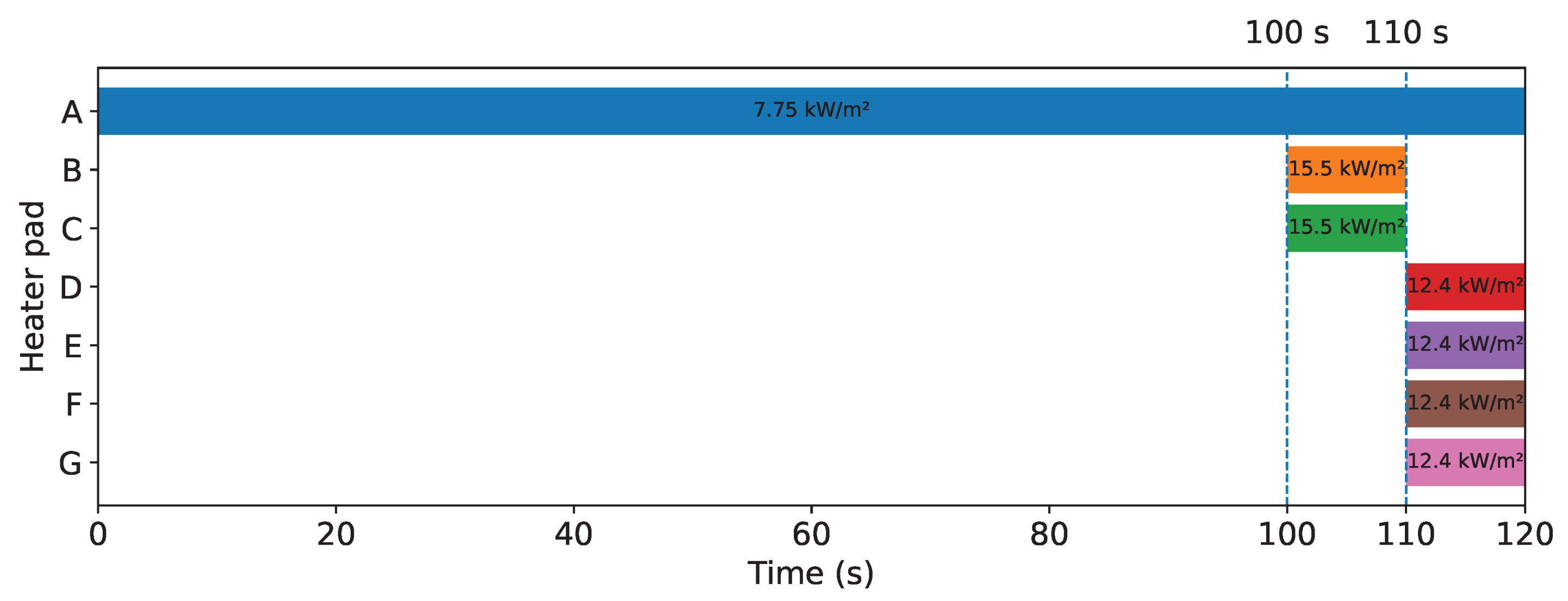
For the heating cycle, all heaters operate in a specific on-off pattern. Each cycle lasts 120 seconds, and the total heating period consists of 5 consecutive cycles, totaling 600 seconds. In the experiment, the start of the heating cycle is precisely synchronized with the initiation of water spray onto the airfoil, meaning the onset of ice accumulation aligns exactly with the beginning of the heating process. To ensure that no ice forms on the leading edge of the airfoil, Heater A remains on continuously throughout the 120-second heating cycle. The other heaters operate cyclically, turning on and off during the heating cycle. The power of each heater and the duration of its operation within each 120-second heating cycle are specified in Table 4.
The different icing cases examined in this study are presented in Table 6. An important point to note is that for cases 1 to 5, where the mean diameter of supercooled droplets is considered to be 20 , a monodisperse distribution has been used, meaning all droplets are assumed to have the same diameter. However, for cases 6 to 8, according to Appendix C and O of the Federal Aviation Regulations (FAR) part 25 [41,42], supercooled large droplets (SLD) are defined as having diameters greater than 40 . Appendix O specifically addresses severe icing conditions, including freezing drizzle and freezing rain, which involve larger supercooled droplets that can create hazardous ice accretion beyond protected surfaces. These conditions are classified as harsh flight environments. For the harsh boundary conditions, supercooled droplets with an MVD of 50 , 100 , and 200 have been used. Unlike the normal conditions, where all droplets were monodisperse, in harsh conditions a Langmuir "D" distribution has been used. The droplet diameters () corresponding to each class (i) and the associated dimensionless ratios and liquid water content weights are summarized in Table 5 [43].

Table 5.
Langmuir “D” distribution Ratios and weight fractions.
| Class i | Ratio /MVD | Weight Fraction [] (%) |
|---|---|---|
| 1 | 0.31 | 5 |
| 2 | 0.52 | 10 |
| 3 | 0.71 | 20 |
| 4 | 1.00 | 30 |
| 5 | 1.37 | 20 |
| 6 | 1.74 | 10 |
| 7 | 2.22 | 5 |
Table 6.
Different cases of icing conditions tested in the present work.
| Case | LWC | MVD | AOA | Roughness Height | Icing Time | ||
|---|---|---|---|---|---|---|---|
| [K] | [m/s] | [g/m3] | [m] | [deg] | [m] | [min] | |
| Normal Flight Condition | |||||||
| Case 1 | 266.483 | 44.704 | 0.78 | 20 | 0 | 500 | 10 |
| Case 2 | 266.483 | 44.704 | 0.78 | 20 | -4 | 500 | 10 |
| Case 3 | 266.483 | 44.704 | 0.78 | 20 | 4 | 500 | 10 |
| Case 4 | 266.483 | 44.704 | 0.78 | 20 | 8 | 500 | 10 |
| Case 5 | 266.483 | 44.704 | 0.78 | 20 | 12 | 500 | 10 |
| Harsh Flight Condition | |||||||
| Case 6 | 266.483 | 44.704 | 0.78 | 50 | 0 | 500 | 10 |
| Case 7 | 266.483 | 44.704 | 0.78 | 100 | 0 | 500 | 10 |
| Case 8 | 266.483 | 44.704 | 0.78 | 200 | 0 | 500 | 10 |
As indicated by Figure 2 and Table 3, heater B is within the impact zone of supercooled droplets and is directly subjected to droplet impingement and ice growth, and thus validation of it with experimental data is extremely critical. On the other hand, Heater D, which is outside the impact zone, may be affected only by runback water flow from the de-icing system, and its simulated results must agree reasonably well with experimental data.
As illustrated in Fig. Figure 4, the performance evaluation of heaters B and D highlights the accuracy and efficiency of the electro-thermal de-icing model. For heater B, the experimental data indicate that the temperature reaches 270 K within 100 s. The results from this study show strong alignment with the experimental trend as well as with other models such as LEWICE [37]. However, the present experiment predicts slightly higher temperatures, with 273 K recorded at 100 s and 292 K at 110 s. The discrepancy could be attributed to differences in the estimation of the water film, which significantly contributes to the thermal behavior in de-icing. Heater B’s temperature then decreases in the cooling regime to around 273 K, closely matching the experimental observation of 271 K. For heater D, which is located outside the impingement zone, the calculated temperature fluctuations also agree well with the experimental data. The present study produced similar results, remaining in close agreement with the measured values, whereas LEWICE overestimated the minimum temperature, leading to a significant discrepancy with the experimental observations.
3. Results and Discussion
3.1. Simulation of Ice Accretion Without De-Icing
In this work, a multi-shot ice accretion simulation technique is utilized to simulate ice accretion on an airfoil. The technique is used by subdividing the overall icing time (e.g., 10 minutes) into smaller intervals (e.g., five 2-minute stages). First, ice accretion is simulated on a clean airfoil for the first interval (2 minutes). Based on the ice profile created on the airfoil’s leading edge, a new geometry for the airfoil is created and the mesh is recreated. The simulation is reiterated for the subsequent 2-minute time interval, considering the modified airfoil geometry resulting from the ice accreted previously. This is an iterative procedure for all the intervals until the entire 10-minute icing time is simulated.
The main advantage of the multi-shot method over a single-shot, 10-minute simulation is that it is more precise. With every stage, the mesh is redefined to reflect the present airfoil shape accurately, particularly in areas of primary interest close to the leading edge. The continuous mesh refinement guarantees that the most critical aerodynamic and thermal phenomena associated with ice accretion are simulated with higher accuracy. Besides, the geometry of ice formed at each stage has a significant influence on the following ice accretion, especially on the forefront, where surface roughness and asymmetry play the most significant roles.
Figure 5 (a) presents the local water droplet collection efficiency on the NACA0012 airfoil in electro-thermal de-icing simulation. For normal icing condition (if angle of attack is ), the collection efficiency reaches a maximum value of 0.54 at the leading edge and decreases to zero when the distance from the leading edge is increased (), since the angle of attack (AOA) is , the curves are symmetrical relative to the upper and lower surfaces of the airfoil, delineating the limits of droplet impingement for a chord position of . As shown in Figure 5 (b), with a transition from normal to harsh SLD conditions, there is a noticeable increase in the collection efficiency at the leading edge, particularly due to the larger supercooled droplet diameter. This leads to a significant expansion of the impingement region. Under normal flight conditions, the impingement limit typically encompasses heaters A, B, and C. However, under harsh conditions, if the MVD is equal to 50 or 100 , heaters A, B, C, D, and E fall within the impingement zone, and as the MVD further increases to 200 , all the heaters are affected.
Figure 6 illustrates the ice accretion profiles on the NACA 0012 airfoil (chord length of 0.9144 m) under the flight and icing conditions specified in Table 6. As shown in Figure 6 (a), with the increase in the angle of attack from -4° to 12°, the amount of ice formed on the leading edge of the airfoil moves more towards the lower surface of the airfoil. As the angle of attack increases, the accumulated ice on the airfoil increases on the lower surface. This expansion of the impingement zone directly influences ice accretion behavior. As depicted in Figure 6 (b), with the increase in the average diameter of the supercooled droplets, the ice thickness on the leading edge remains relatively unchanged, but the ice progression along the chord of the airfoil becomes more pronounced on both the upper and lower surfaces. This phenomenon is closely tied to droplet impact zone and collection efficiency, as the larger droplet diameters enhance droplet break-up, splashing, and bouncing, thereby intensifying the spread of ice formation.
3.2. Aerodynamics Degradation
Ice buildup on the leading edge of an airfoil significantly affects its aerodynamic performance by disrupting the smooth airflow, increasing drag, and reducing lift. he altered leading-edge geometry promotes premature boundary-layer separation; the flow becomes turbulent and forms a separated vortex downstream of the ice, particularly on the suction side, as show in Figure 7 for case 1. This separation slows down the airflow, raises pressure, and causes a sharp drop in lift. The accompanying rise in drag further reduces efficiency and increases fuel consumption.
Studies show that the lift coefficient can decrease by up to [6], while drag can increase by as much as 36% to 200% [44]. These changes, influenced by factors such as temperature and the duration of ice accretion, not only degrade aerodynamic performance but also create significant safety risks, including the potential for loss of control.
As shown in Table 7, under normal flight conditions, an increase in the angle of attack causes a decrease in the lift coefficient and an increase in the drag coefficient. The worst condition is achieved at an angle of attack of , with the lift coefficient decreasing by 11.1% and the drag coefficient increasing by 48.2%. In harsh flight conditions, with the angle of attack fixed at , the lift coefficient remains essentially unchanged as the median volume diameter (MVD) of supercooled droplets increases, whereas the drag coefficient rises markedly by at an MVD of 200 m.
3.3. Analysis of electro-thermal de-icing system in normal icing conditions
When supercooled droplets in the air collide with the wings and body of an aircraft under normal conditions, they form a layer of ice. However, with the use of electro-thermal de-icing systems, heaters embedded beneath the wing surface warm the surface, causing the accumulated ice to melt and form a thin film of water. This thin water layer is pushed backward over the wing by airflow, and if these new areas are not thermally protected by the de-icing system, the water refreezes and forms ice. The concept of cyclic electro-thermal de-icing involves multiple heaters with varying power densities and lengths installed at different locations inside the wing, directly beneath its surface. These heaters operate cyclically, turning on and off in sequence. The de-icing process thus includes a combination of ice accumulation, ice melting, water film dynamics, and refreezing, which can lead to ice accumulation at various locations on the airfoil surface.
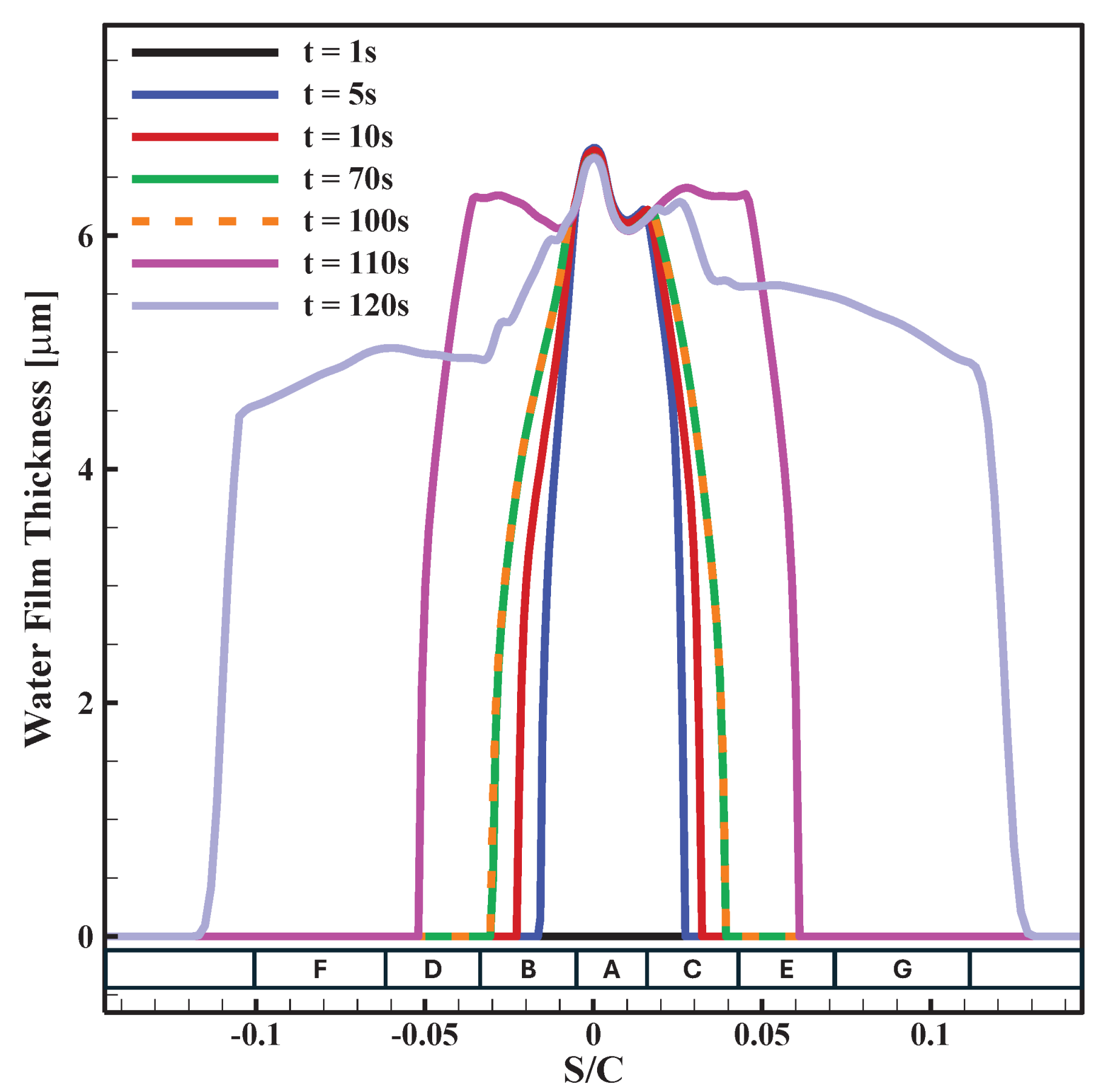
During the cyclic de-icing process, ice accretion can occur in various locations due to the presence of water from melting ice and the runback water film. In the first 100 seconds, when only heater A is on, the ice accretion process begins on the airfoil surface, which has a low initial temperature. As shown in Figure 8; immediately after heater A is turned on, the surface temperature remains below the freezing point (=273.15 K). It takes about 5 seconds for the surface temperature to reach , causing the supercooled water droplets (initially) to freeze instantly, without any runback water. As time passes, the heat power from heater A gradually raises the surface temperature, melting the ice layer and preventing further freezing in the heated area. Eventually, the surface temperature over heater A rises above the freezing point, preventing any ice formation in this area and creating a thin water film with a thickness of just a few microns. As a result, the volume of runback water generated increases, and it flows toward heaters B and C, leading to continued ice accumulation over heaters B and C (as shown in Figure 10 & Figure 12). Between 10 and 70s, the width of the water film continues to expand (Figure 9). By 70s, the surface temperature differences stabilize, and the ice thickness growth becomes steady (Figure 10), indicating that the thermal equilibrium of the icing process is approaching a steady state. During this period, although the width of the liquid film remains unchanged, the ice thickness over heaters B and C continues to increase significantly (as shown in Figure 10 & Figure 12).
Additionally, since the initial temperature of the entire airfoil surface is set to the static ambient temperature at the start of the simulation, the boundary layer temperature around the wing gradually rises due to electro-thermal heating. As shown in Figure 8, the surface temperature in areas outside the influence of water droplets and heaters (surfaces with no heater underneath) increases gradually over time due to convective heat transfer from the air, as also noted in the study by [40].
After 100 s, when heaters B and C are turned on (see timing diagram Figure 11), their heat raises the outer surface temperatures, initiating the melting of ice accumulated during the first 100 seconds over these heaters. As shown in Figure 9 & Figure 12, the width of the water film expands along the airfoil chord over areas D and E, indicating that the ice on heaters B and C is melting. At 110 seconds, heaters D, E, F, and G are turned on while heaters B and C are switched off. Within a short time, the surface temperatures in the areas of heaters B and C drop to the freezing point (Figure 4). Meanwhile, the water film flows downstream over heaters D, E, F, and G between 110 and 120 seconds, covering a wide area on the airfoil surface, as illustrated in Figure 9 and Figure 12.
Figure 9.
Water film thickness distributions at different times in the de-icing process
Since the ice on these heaters melts, the liquid film flows beyond the areas of heaters F and G and begins to freeze again in unprotected regions, forming ice ridges, as shown in Figure 10 & Figure 12. Regarding the formation and movement of the water film, it is assumed that the water layer fully wets the surface. However, the continuous flow of the water layer outside the impingement limit may break into small rivulets or even separate droplets due to hydrodynamic instabilities in the water film [45].
3.4. Analysis of Electro-Thermal De-Icing System at Various Angles of Attack
As shown in Figure 13, for the airfoil surface related to heater A, for small angles of attack, ice accretion on the leading edge of the airfoil occurs only during the first 5 seconds when the surface temperature has not yet reached the ice melting temperature (). After this initial period, due to the continuous operation of heater A, the surface temperature rises above , causing the average ice thickness to nearly reach zero. However, for larger angles of attack, such as or , some ice accretion still occurs on the leading edge of the airfoil despite the heater being continuously active. Specifically, for , ice accretion persists up to 100 s, while for , it persists throughout the entire period of 600s. At higher angles of attack, the thermal load on the upper leading edge increases beyond the heater capacity. This indicates that even when the heater operates continuously, at , the system is not able to fully melt the whole ice in this region. This can be interpreted as follows: as angle of attack () increases, higher local velocities raise the convective heat-transfer coefficient , enhancing cooling. The local energy balance, , may therefore not be satisfied at , so does not remain above and leading-edge ice persists throughout the 600 s window. At , the same heater overcomes these losses, and the surface becomes essentially ice-free after the first few seconds. Although the average ice thickness at is small, even minor ice accretion can degrade aerodynamic performance and increase surface roughness.
Figure 10.
Ice thickness distributions at different times in the de-icing process.
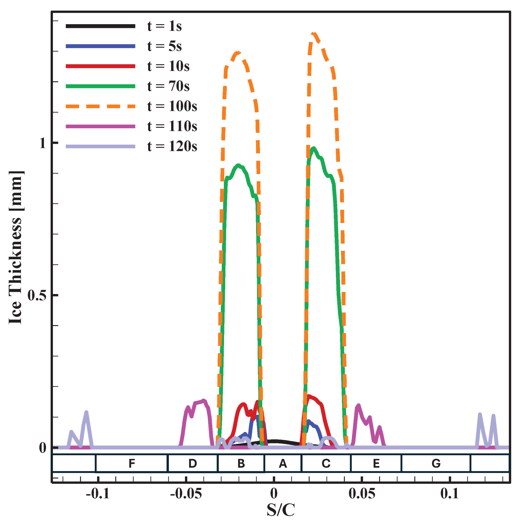
Figure 11.
Heater activation timing.
For the surface above heater B, performance is best at , where the average ice thickness decays toward zero. Moving away from degrades performance—most notably at —because the imposed thermal load during the accumulation phase of each 120 s cycle increases. In all nonzero angles, the first cycle shows the largest build-up, but subsequent cycles exhibit progressively lower peaks, indicating that the periodic heating is largely effective over time. Over heater C the system is effective at : a sizable build-up appears in the first cycle, but the average thickness decreases as cycles proceed. At and the trend reverses. Early cycles show modest accumulation, yet the average thickness grows in later cycles. This is consistent with runback water produced upstream (primarily above heater A) re-freezing near the heater-C footprint, where the available power density is insufficient to fully melt it during the cycle. A thin residual layer then remains at the end of each cycle and compounds over time. Improving high- performance will require re-balancing power or modifying the heater layout in this region (e.g., extended length or higher local heat flux).
Figure 12.
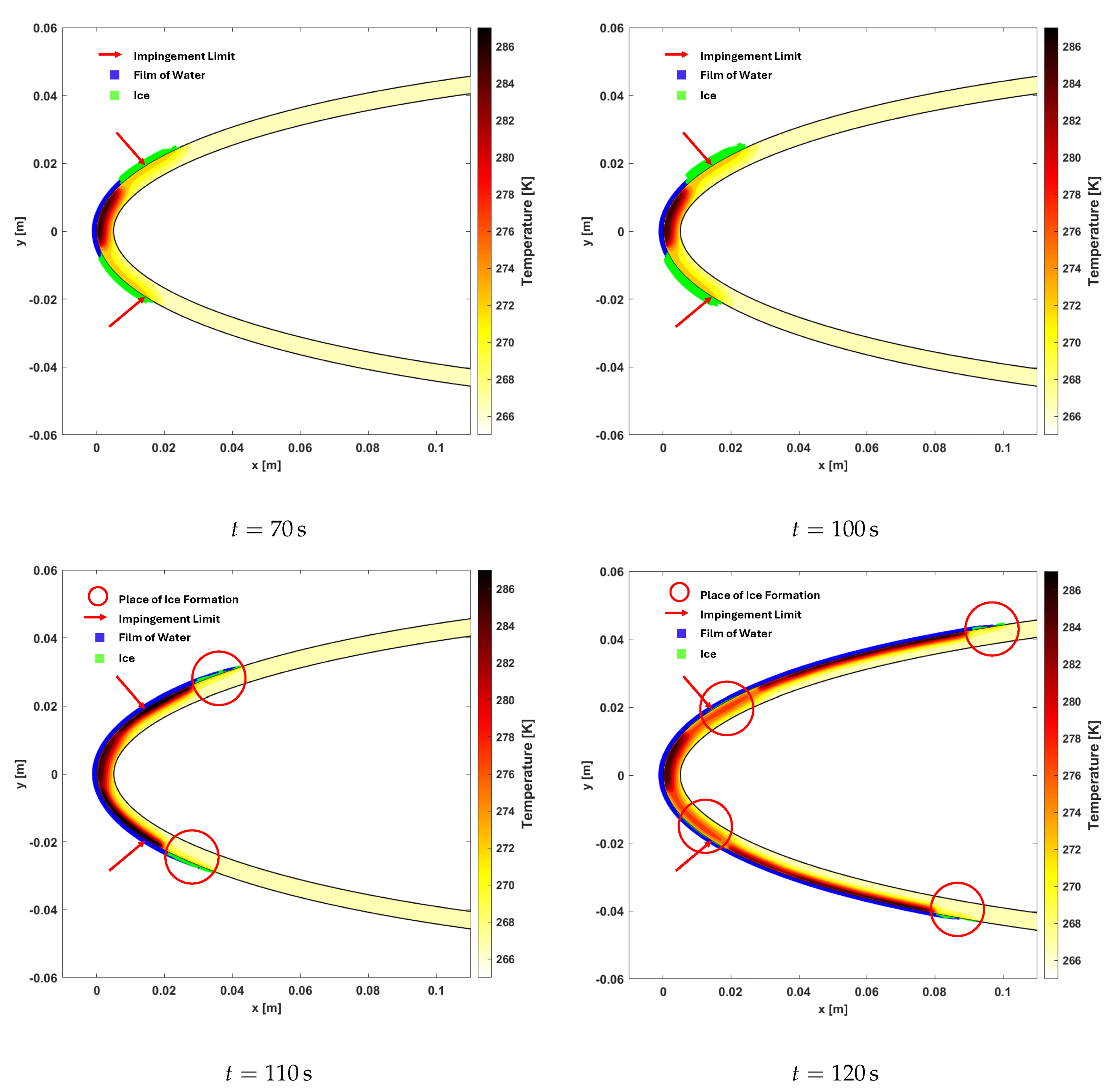
Film of water, ice profile, and temperature contours at different times. To improve visibility, the height of the water film and ice have been increased by a factor of 200 and 2, respectively.
Figure 12.
Film of water, ice profile, and temperature contours at different times. To improve visibility, the height of the water film and ice have been increased by a factor of 200 and 2, respectively.
Above heater E, performance is weak at and ; for higher angles the instantaneous accretion rate is lower than at small , but the average thickness still increases monotonically over time. Only at is a net reduction observed. Because this zone lies farther downstream on the suction surface, its aerodynamic penalty is smaller than that of the leading-edge regions, yet the persistent growth indicates that additional coverage or power would be beneficial. Finally, above heater G, higher angles () yield negligible accretion compared with and . Some ice does accumulate over time, but the amounts remain small; at , however, the end-of-cycle thickness is appreciable. For the thermally unprotected airfoil upper surface, which is located downstream of heater G, no ice accumulates during the de-icing cycle at an angle of attack of . However, at other angles of attack, especially at , the amount of accumulated ice increases over time as expected, due to the increase in the runback water film. Nevertheless, the average ice thickness formed in this region remain small and aerodynamically insignificant over the simulated duration.
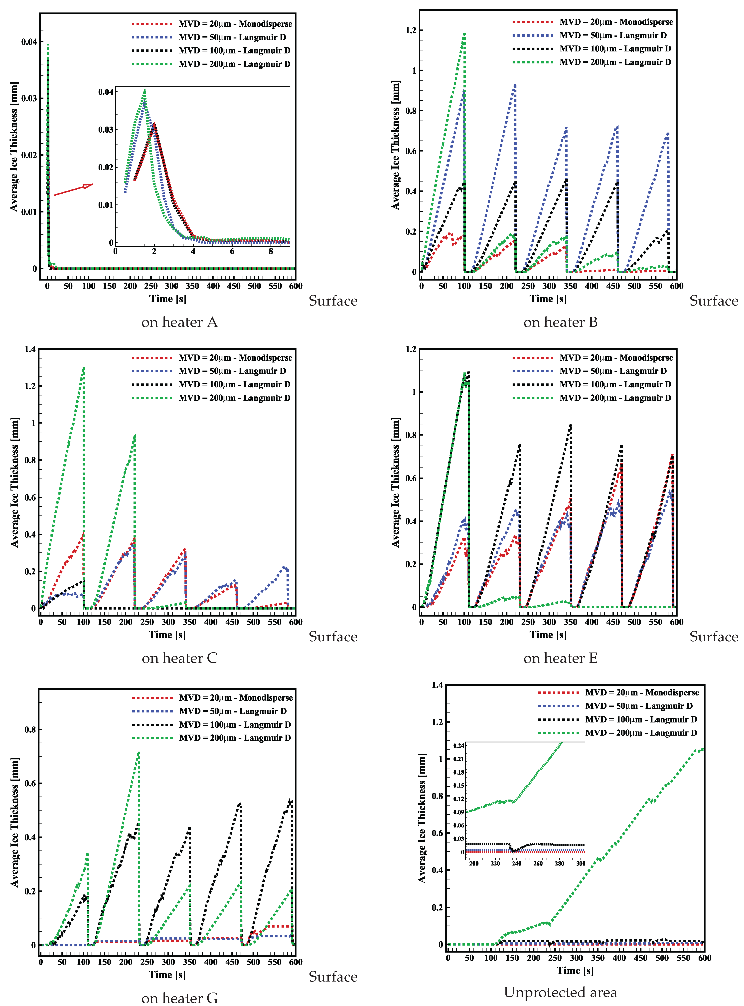
3.5. Analysis of Electro-Thermal De-Icing System in Harsh SLD Condition
Figure 14 compares normal icing (monodisperse) with SLD conditions represented by Langmuir D distribution (MVD=50 m, 100 m, 200 m). Above heater A (continuous operation), only a brief < 5 s accretion occurs before the surface exceeds . By 600 s the leading-edge average thickness is near zero in both normal and SLD conditions, indicating robust protection at this critical location. Because of the asymmetric internal layout, heaters B and C do not behave identically. Over heater B the lowest performance occurs for MVD=50m: the average ice thickness remains roughly constant through time, which is undesirable given its proximity to the leading edge. For MVD m, a large initial build-up appears in the first ∼ 100 s, but subsequent cycles reduce the average thickness to near zero by the end of the simulation. For the airfoil surface associated with heaters C the behavior for MVD m is similar—high early accumulation followed by gradual removal to near zero. Unlike heater B, heater C handles MVD m more effectively, reducing the average thickness throughout the cycles. Given that heater C covers part of the suction surface, this improved response is particularly important for aerodynamic performance. However, on heater E the response to MVD m, m, and m is unsatisfactory: the average thickness remains nearly constant or increases with time. Although this region is farther from the leading edge (so its aerodynamic impact is smaller than for A/B/C), the monotonic growth indicates that additional coverage or power reallocation would help. On heater G the system performs well for MVD m (normal icing conditions) and m, but poorly for m and m, where the average thickness is nearly steady or increasing.
In the thermally unprotected zone downstream of heater G, the response is acceptable for m, m, and m: after ∼ 100 s, runback film entering this region causes a small increase in average thickness, but the values remain low. In stark contrast, m droplets produce a sustained increase throughout the cycle, posing a clear hazard. With no installed heaters, ice can grow to significant thickness and mass, raising the risk of ice shedding and potential damage to downstream surfaces. The results argue for chordwise coverage (more/longer heaters) and/or higher local power density for electro-thermal de-icing in harsh SLD conditions. Consequently, alternative or hybrid strategies, such as combining passive and active methods, should be considered for better performance.
Figure 13.
Comparison of average ice thickness at different angles of attack, Case 1 to Case 5.
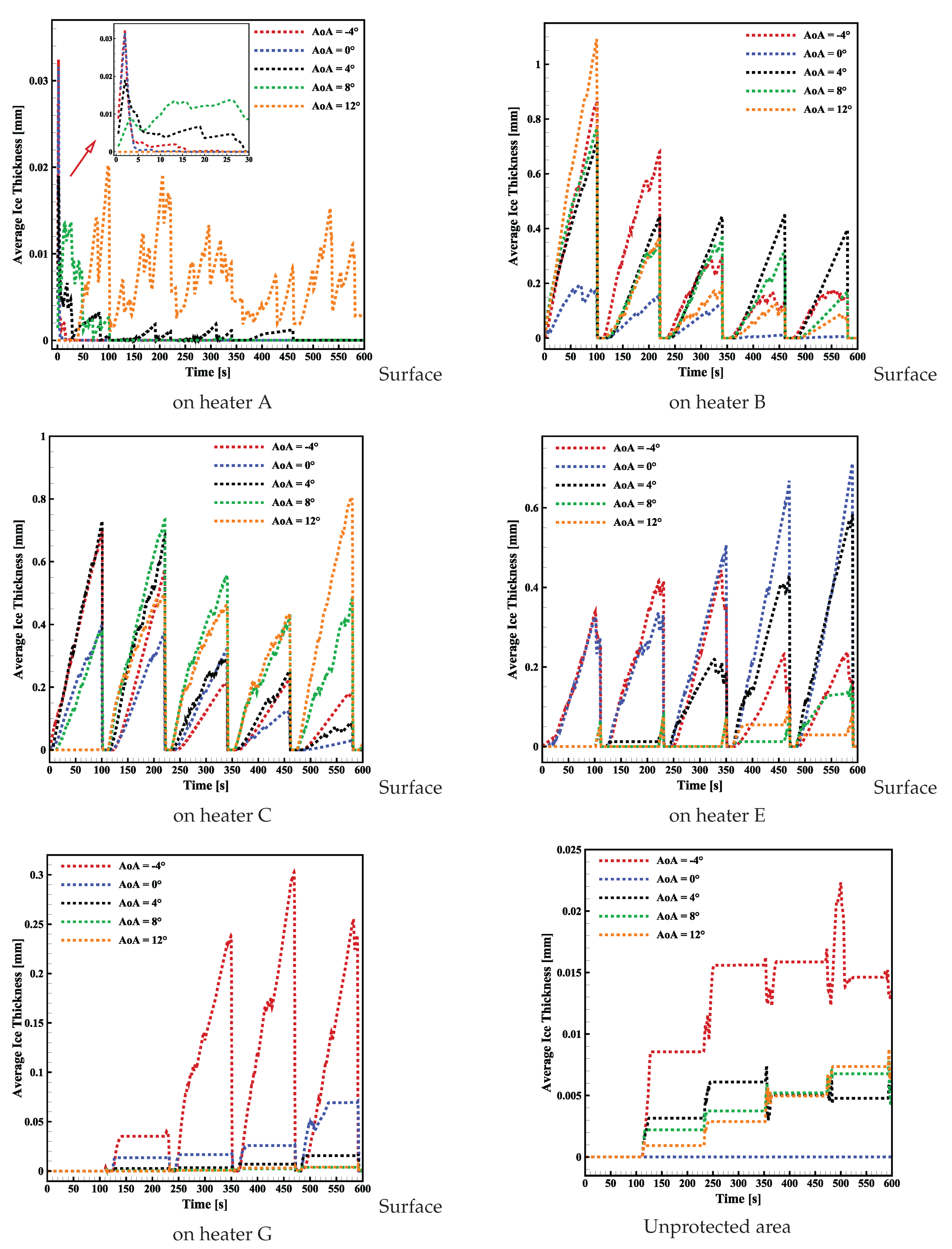
Figure 14.
Comparison of average ice thickness at different supercooled droplet sizes: Case 1 and Cases 6 to 8.
Figure 14.
Comparison of average ice thickness at different supercooled droplet sizes: Case 1 and Cases 6 to 8.
4. Conclusion
This study performed a comprehensive simulation of ice accretion and electro-thermal de-icing on an airfoil under various icing conditions. Accretion was first modeled for 10 minutes using a multi-shot approach that captured geometry changes due to ice build-up. The resulting aerodynamic penalties were significant: at an angle of attack 12°, the lift coefficient decreased by over 10% and the drag coefficient increased by almost 50%. Under SLD conditions with a median volume diameter (MVD) of 200 m, the drag coefficient increased by more than 30%. These results confirm the detrimental impact of icing on performance and underscore the need for effective de-icing strategies.
A cyclic electro-thermal de-icing system (five 2-minute cycles) was then simulated. The model, which shows good agreement with available experimental and numerical data, reproduced heat-transfer processes during freezing, melting, and evaporation. When the leading-edge heater was activated during supercooled droplet impingement for less than 5 s, a thin ice layer formed due to subfreezing surface temperatures but subsequently melted. As the cycle progressed, a water film developed and remained stable for approximately 70 s until downstream heaters are activated, after which runback water refroze in unprotected regions, forming ice ridges. While the baseline assumed monodisperse droplets of (20 m), larger SLD (>40 m) would alter collection efficiency and impingement behavior, highlighting the sensitivity of de-icing outcomes to droplet size.
Performance varied with angle of attack and SLD conditions as a function of heater placement. At small angles of attack, leading-edge accretion was minimal under continuous operation of Heater A, with ice thickness approaching zero after an initial transient. At higher angles, however, ice accumulation persisted despite continuous heating, indicating limitations in fully eliminating accretion in critical aerodynamic regions. Under SLD conditions, Heaters A and C were relatively effective, whereas Heaters B, E, and G were less effective, particularly for larger droplets of over 50 m. For 200 m droplets, ice thickness increased substantially in thermally unprotected areas—an operational hazard due to both ice accumulation and potential shedding. These observations point to the value of additional or longer heaters to extend thermal protection under challenging conditions. Finally, as a prospective alternative and complement to electro-thermal configurations (revised heater sizing and placement), passive icephobic coatings should be explored to improve runback management and reduce refreezing.
Author Contributions
Conceptualization, M.T. and S.G.N.; methodology, M.T. and S.G.N.; software, S.G.N.; validation, S.G.N.; formal analysis, M.T. and S.G.N.; investigation, S.G.N. and M.T; resources, M.T.; data curation, S.G.N.; writing—original draft preparation, S.G.N.; writing—review and editing, M.T.; visualization, S.G.N.; supervision, M.T.; project administration, M.T.; funding acquisition, M.T. All authors have read and agreed to the published version of the manuscript.
Funding
This research received no external funding.
Institutional Review Board Statement
Not applicable.
Informed Consent Statement
Not applicable.
Data Availability Statement
Data are contained within the article.
Acknowledgments
The authors thank the journal staff for their comments and revisions to this paper.
Conflicts of Interest
The authors declare no conflicts of interest.
Nomenclature
The following symbols and abbreviations are used in this manuscript:
| Parameters | |
| Convective heat-transfer coefficient [W ] | |
| Specific heat [J ] | |
| Energy of droplet [J] | |
| h | Thickness [m] |
| L | Latent heat [J kg] |
| LWC | Liquid water content [kg ] |
| Mass transfer rate [kg s] | |
| Q | Heat flux [W m] |
| T | Temperature [K] |
| Mean velocity [m s] | |
| Velocity vector [m ] | |
| Water volume fraction | |
| Weber number | |
| Ohnesorge number | |
| Droplet’s surface tension | |
| Mundo parameter | |
| Cossali parameter | |
| Boltzmann constant [W ] | |
| Solid emissivity | |
| Collection efficiency | |
| Froude Number | |
| Drag coefficient | |
| Droplet Reynolds number | |
| K | Inertial parameter |
| Dynamic viscosity [Pa s] | |
| Wall shear stress [Pa] | |
| Enthalpy change [J] | |
| S | Curvilinear arc length along the airfoil surface from the leading-edge [m] |
| C | Chord length (leading edge to trailing edge) [m] |
| Subscripts | |
| a | Air |
| d | Droplet |
| evap | Evaporation |
| f | Water film |
| rec | Recovery |
| ∞ | Reference (freestream) |
References
- Cao, Y.; Tan, W.; Wu, Z. Aircraft icing: An ongoing threat to aviation safety. Aerospace science and technology 2018, 75, 353–385. [Google Scholar] [CrossRef]
- Kong, W.; Liu, H. Unified icing theory based on phase transition of supercooled water on a substrate. International Journal of Heat and Mass Transfer 2018, 123, 896–910. [Google Scholar] [CrossRef]
- Zhao, Y.; Guo, Q.; Lin, T.; Cheng, P. A review of recent literature on icing phenomena: Transport mechanisms, their modulations and controls. International Journal of Heat and Mass Transfer 2020, 159, 120074. [Google Scholar] [CrossRef]
- Bourgault, Y.; Beaugendre, H.; Habashi, W.G. Development of a shallow-water icing model in FENSAP-ICE. Journal of Aircraft 2000, 37, 640–646. [Google Scholar] [CrossRef]
- Nath, P.; Lokanathan, N.; Wang, J.; Benmeddour, A.; Nichman, L.; Ranjbar, K.; Hickey, J.P. Parametric investigation of aerodynamic performance degradation due to icing on a symmetrical airfoil. Physics of Fluids 2024, 36. [Google Scholar] [CrossRef]
- Lu, H.; Xu, Y.; Li, H.; Zhao, W. Numerical study on glaze ice accretion characteristics over time for a NACA 0012 airfoil. Coatings 2023, 14, 55. [Google Scholar] [CrossRef]
- Esmaeilifar, E.; Raj, L.P.; Myong, R. Computational simulation of aircraft electrothermal de-icing using an unsteady formulation of phase change and runback water in a unified framework. Aerospace Science and Technology 2022, 130, 107936. [Google Scholar] [CrossRef]
- Rausa, A.; Guardone, A. Multi-physics simulation of in-flight ice shedding. In Proceedings of the Journal of Physics: Conference Series. IOP Publishing, 2021, Vol. 1730, p. 012024.
- Sengupta, B.; Raj, L.P.; Cho, M.; Son, C.; Yoon, T.; Yee, K.; Myong, R. Computational simulation of ice accretion and shedding trajectory of a rotorcraft in forward flight with strong rotor wakes. Aerospace Science and Technology 2021, 119, 107140. [Google Scholar] [CrossRef]
- Farabello, L.; Scarabino, A.; Bacchi, F. Numerical analysis of ice accretion on an airfoil: A case study. Revista Facultad de Ingeniería Universidad de Antioquia 2025.
- Mousavi, S.M.; Sotoudeh, F.; Chun, B.; Lee, B.J.; Karimi, N.; Faroughi, S.A. The potential for anti-icing wing and aircraft applications of mixed-wettability surfaces-A comprehensive review. Cold Regions Science and Technology 2024, 217, 104042. [Google Scholar] [CrossRef]
- Janjua, Z.A.; Turnbull, B.; Hibberd, S.; Choi, K.S. Mixed ice accretion on aircraft wings. Physics of Fluids 2018, 30. [Google Scholar] [CrossRef]
- Bodoc, V.; Berthoumieu, P.; Déjean, B. Experimental investigation of large droplet impact with application to SLD icing. Microgravity Science and Technology 2021, 33, 59. [Google Scholar] [CrossRef]
- Zhang, C.; Wang, F.; Kong, W.; Liu, H. The Characteristics of SLD icing accretions and aerodynamic effects on high-lift configurations. In Proceedings of the 33rd AIAA Applied Aerodynamics Conference; 2015; p. 3385. [Google Scholar]
- Yamazaki, M.; Jemcov, A.; Sakaue, H. A review on the current status of icing physics and mitigation in aviation. Aerospace 2021, 8, 188. [Google Scholar] [CrossRef]
- Lee, J.W.; Cho, M.Y.; Kim, Y.H.; Yee, K.; Myong, R.S. Current status and prospect of aircraft ice protection systems. Journal of the Korean Society for Aeronautical & Space Sciences 2020, 48, 911–925. [Google Scholar] [CrossRef]
- Gallia, M.; Carnemolla, A.; Premazzi, M.; Guardone, A. Optimisation of a Nacelle Electro-Thermal Ice Protection System for Icing Wind Tunnel Testing. Transactions on Aerospace Research 2023, 2023, 32–44. [Google Scholar] [CrossRef]
- Tormen, D.; Zanon, A.; De Gennaro, M. Ice Protection System Design for the Next Generation Civil Tiltrotor Engine Intake. Technical report, SAE Technical Paper, 2023.
- Hann, R.; Enache, A.; Nielsen, M.C.; Stovner, B.N.; van Beeck, J.; Johansen, T.A.; Borup, K.T. Experimental heat loads for electrothermal anti-icing and de-icing on UAVs. Aerospace 2021, 8, 83. [Google Scholar] [CrossRef]
- Shi, K.; Duan, X. A review of ice protection techniques for structures in the Arctic and offshore harsh environments. Journal of Offshore Mechanics and Arctic Engineering 2021, 143, 064502. [Google Scholar] [CrossRef]
- Pourbagian, M.; Habashi, W. On Optimal Design of Electro-Thermal In-Flight Ice Protection Systems. In Proceedings of the 5th AIAA Atmospheric and Space Environments Conference; 2013; p. 2937. [Google Scholar]
- Gallia, M.; Rausa, A.; Martuffo, A.; Guardone, A. A comprehensive numerical model for numerical simulation of ice accretion and electro-thermal ice protection system in anti-icing and de-icing mode, with an ice shedding analysis. Technical report, SAE Technical Paper, 2023.
- He, Z.; Wang, J. Anti-icing strategies are on the way. The Innovation 2022, 3. [Google Scholar] [CrossRef]
- He, Z.; Xie, H.; Jamil, M.I.; Li, T.; Zhang, Q. Electro-/Photo-Thermal Promoted Anti-Icing Materials: A New Strategy Combined with Passive Anti-Icing and Active De-Icing. Advanced Materials Interfaces 2022, 9, 2200275. [Google Scholar] [CrossRef]
- Mauery, T.; Alonso, J.; Cary, A.; Lee, V.; Malecki, R.; Mavriplis, D.; Medic, G.; Schaefer, J.; Slotnick, J. A guide for aircraft certification by analysis. Technical report, 2021.
- Gutiérrez, B.A.; Della Noce, A.; Gallia, M.; Bellosta, T.; Guardone, A. Numerical simulation of a thermal Ice Protection System including state-of-the-art liquid film model. Journal of Computational and Applied Mathematics 2021, 391, 113454. [Google Scholar] [CrossRef]
- Bennani, L.; Trontin, P.; Radenac, E. Numerical simulation of an electrothermal ice protection system in anti-icing and deicing mode. Aerospace 2023, 10, 75. [Google Scholar] [CrossRef]
- Niu, Y.; Wang, Z.; Su, J.; Yao, J.; Wang, H. Prediction of Airfoil Icing and Evaluation of Hot Air Anti-Icing System Effectiveness Using Computational Fluid Dynamics Simulations. Aerospace 2025, 12. [Google Scholar] [CrossRef]
- Stewart, E.A.; Bartkus, T.P. Computational Icing Analysis on NASA’s SIDRM Geometry to Investigate Collection Efficiency. In Proceedings of the International Conference on Icing of Aircraft, Engines, and Structures; 2023. [Google Scholar]
- Uranai, S.; Fukudome, K.; Mamori, H.; Fukushima, N.; Yamamoto, M. Numerical simulation of the anti-icing performance of electric heaters for icing on the NACA 0012 airfoil. Aerospace 2020, 7, 123. [Google Scholar] [CrossRef]
- Milani, Z.R.; Matida, E.; Razavi, F.; Ronak Sultana, K.; Timothy Patterson, R.; Nichman, L.; Benmeddour, A.; Bala, K. Numerical Icing Simulations of Cylindrical Geometry and Comparisons to Flight Test Results. Journal of Aircraft 2024, pp. 1–11.
- Martini, F.; Ibrahim, H.; Contreras Montoya, L.; Rizk, P.; Ilinca, A. Turbulence modeling of iced wind turbine airfoils. Energies 15 (22): 8325, 2022.
- Esmaeilifar, E.; Sengupta, B.; Raj, L.P.; Myong, R. In-flight anti-icing simulation of electrothermal ice protection systems with inhomogeneous thermal boundary condition. Aerospace Science and Technology 2024, 150, 109210. [Google Scholar] [CrossRef]
- Papadakis, M.; Wong, S.C.; Rachman, A.; Hung, K.E.; Vu, G.T.; Bidwell, C.S. Large and small droplet impingement data on airfoils and two simulated ice shapes. Technical report, 2007.
- Ansys. Ansys FENSAP-ICE User Manual, Release 2022 R2. Ansys, Canonsburg, PA, 2022. 2022.
- Aupoix, B.; Spalart, P. Extensions of the Spalart–Allmaras turbulence model to account for wall roughness. International Journal of Heat and Fluid Flow 2003, 24, 454–462. [Google Scholar] [CrossRef]
- Wright, B.; Al-Khalil, K.; Miller, D. Validation of nasa thermal ice protection computer codes part2-lewice. Thermal, AIAA 1997, pp. 97–0050.
- Zhou, Z.; Li, F.; Li, G.; Sang, W. Icing numerical simulation for single and multi-element airfoils. In Proceedings of the 28th AIAA Applied Aerodynamics Conference; 2010; p. 4232. [Google Scholar]
- Costes, M.; Moens, F.; Brunet, V. Prediction of iced airfoil aerodynamic characteristics. In Proceedings of the 54th AIAA Aerospace Sciences Meeting; 2016; p. 1547. [Google Scholar]
- Shen, X.; Wang, H.; Lin, G.; Bu, X.; Wen, D. Unsteady simulation of aircraft electro-thermal deicing process with temperature-based method. Proceedings of the Institution of Mechanical Engineers, Part G: Journal of Aerospace Engineering 2020, 234, 388–400. [Google Scholar] [CrossRef]
- Federal Aviation Administration. CFR Part 25 Appendix C. Federal Register Rules and Regulations, 2011.
- Federal Aviation Administration. Airplane and Engine Certification Requirements in Supercooled Large Drop, Mixed Phase, and Ice Crystal Icing Conditions. Federal Register Rules and Regulations, 2014.
- Langmuir, I.; Blodgett, K. A mathematical investigation of water droplet trajectories; Number 5418, Army Air Forces Headquarters, Air Technical Service Command, 1946.
- Yang, X.; Bai, X.; Cao, H. Influence analysis of rime icing on aerodynamic performance and output power of offshore floating wind turbine. Ocean Engineering 2022, 258, 111725. [Google Scholar] [CrossRef]
- Suzzi, N.; Croce, G. Numerical simulation of film instability over low wettability surfaces through lubrication theory. Physics of Fluids 2019, 31. [Google Scholar] [CrossRef]
Figure 1.
Flowchart of the unsteady icing/de-icing simulation.
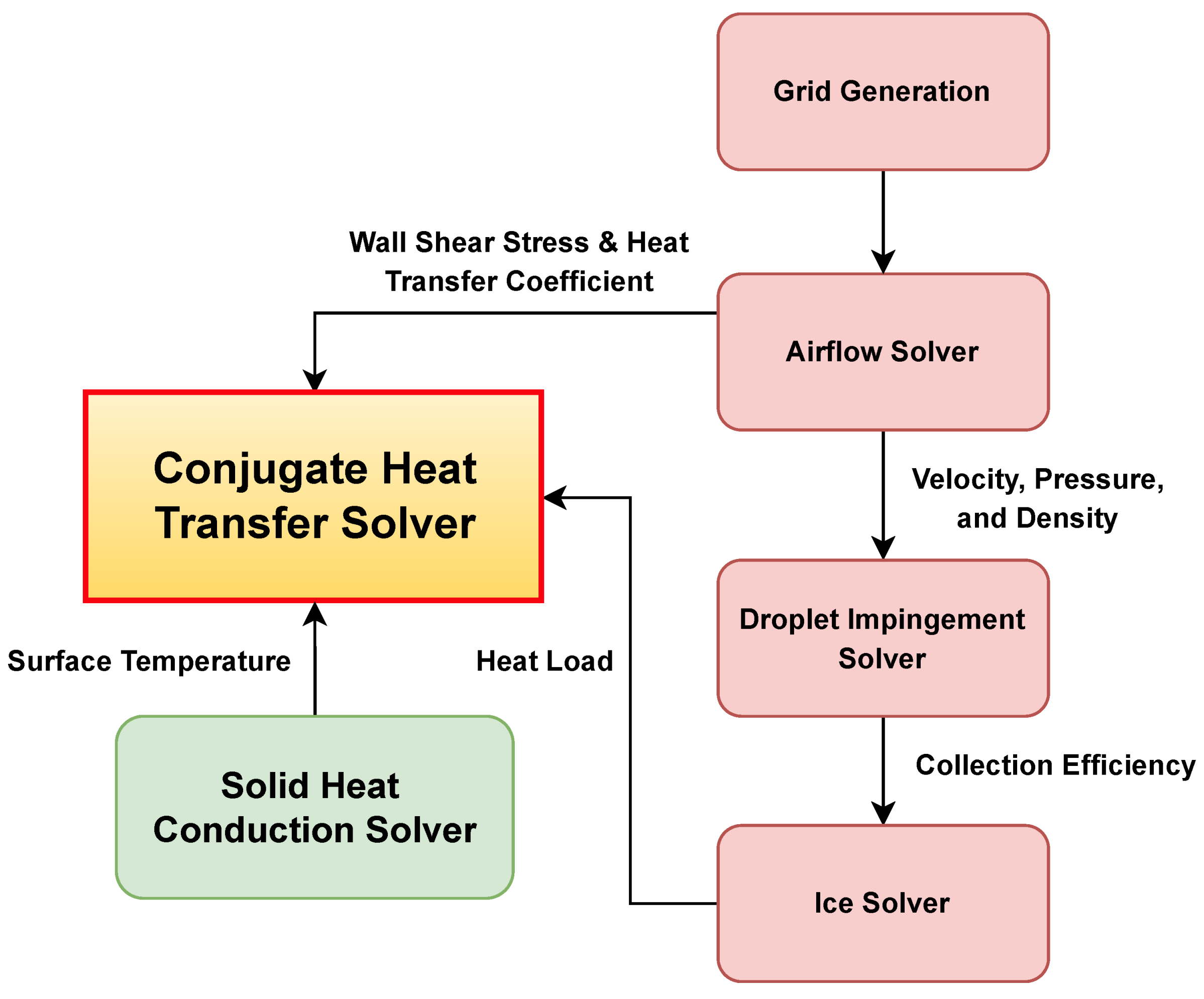
Figure 2.
Geometry and heaters of the electro-thermal de-icing system.
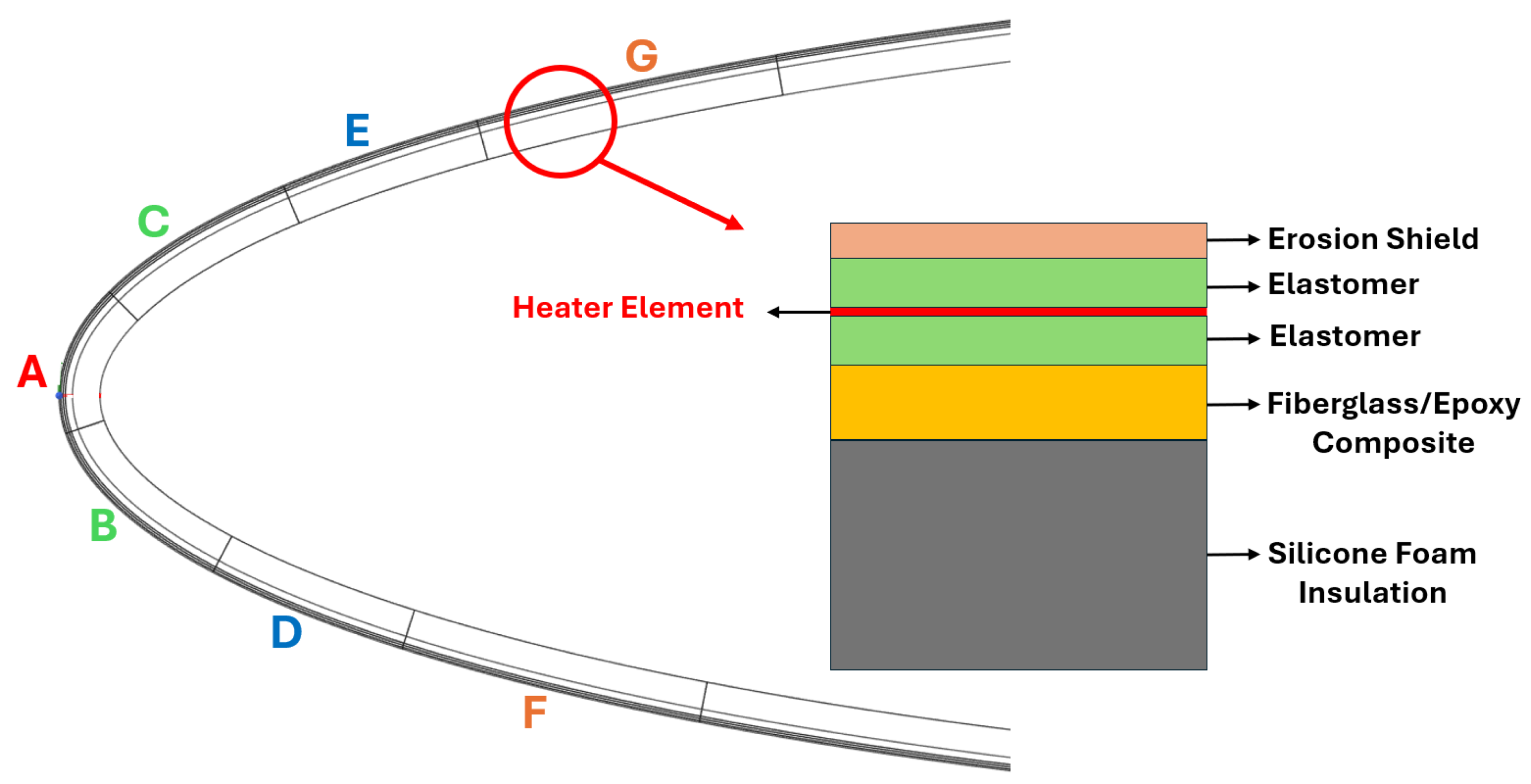
Figure 3.
Computational fluid and solid domain.
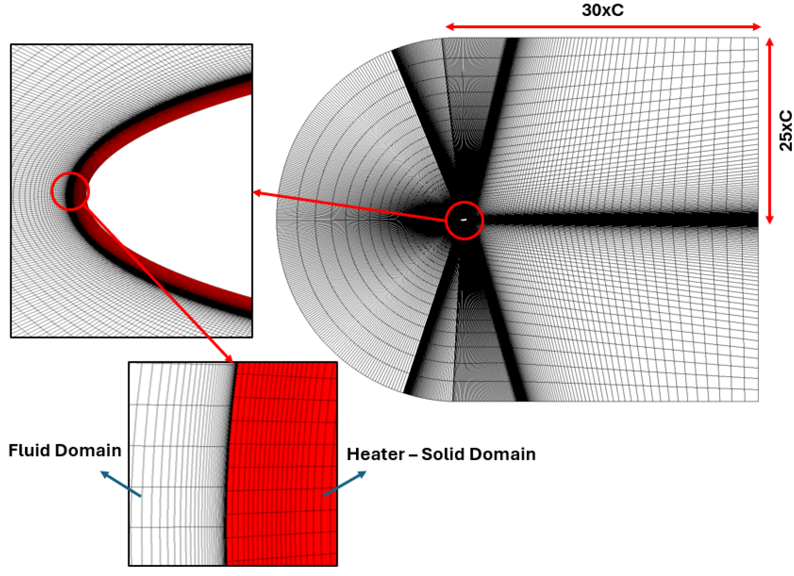
Figure 4.
Comparison of temperature change over time at (a) heater B, (b) heater D.
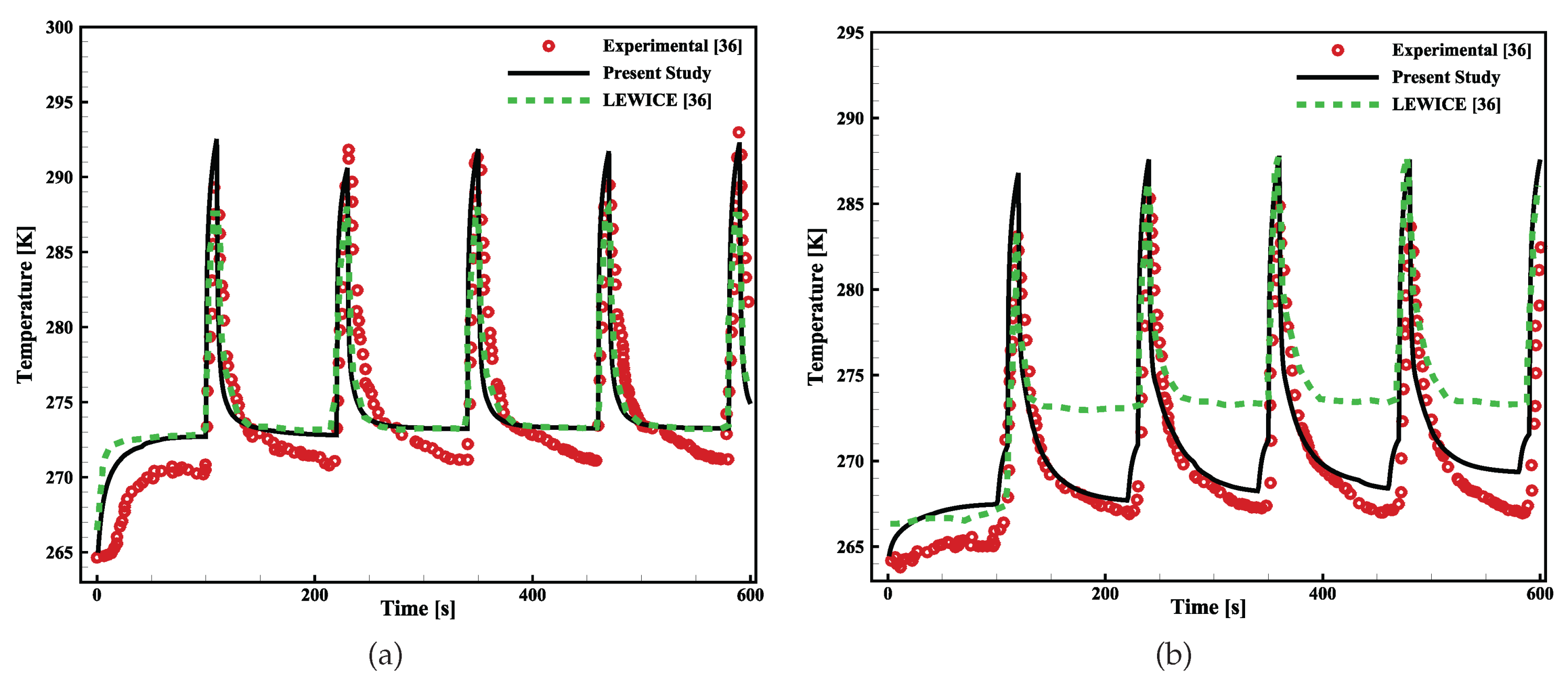
Figure 5.
Collection efficiency at and : (a) Normal flight condition with monodispersed MVD = 20 m at different AOA; (b) Harsh flight condition with Langmuir D distribution of MVD = 50, 100, and 200 m.
Figure 5.
Collection efficiency at and : (a) Normal flight condition with monodispersed MVD = 20 m at different AOA; (b) Harsh flight condition with Langmuir D distribution of MVD = 50, 100, and 200 m.
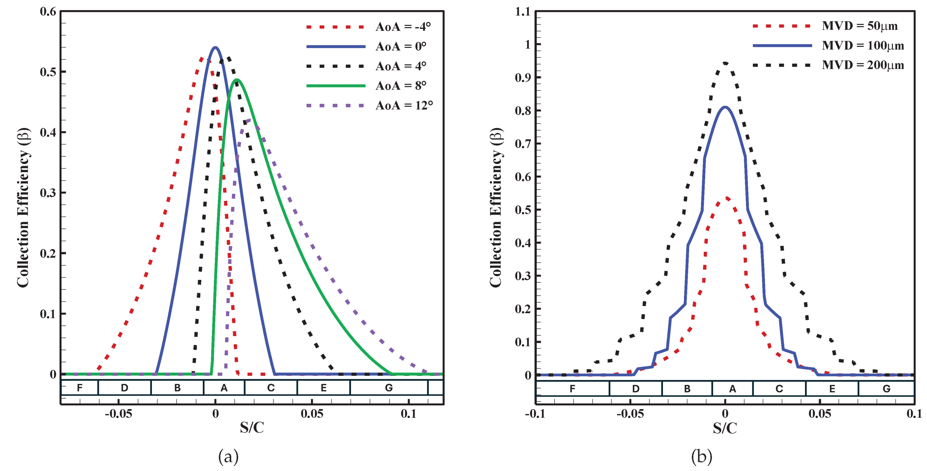
Figure 6.
Ice accretion profiles: (a) Normal flight condition, all cases with MVD = 20 m at different AoA; (b) Harsh flight condition.
Figure 6.
Ice accretion profiles: (a) Normal flight condition, all cases with MVD = 20 m at different AoA; (b) Harsh flight condition.
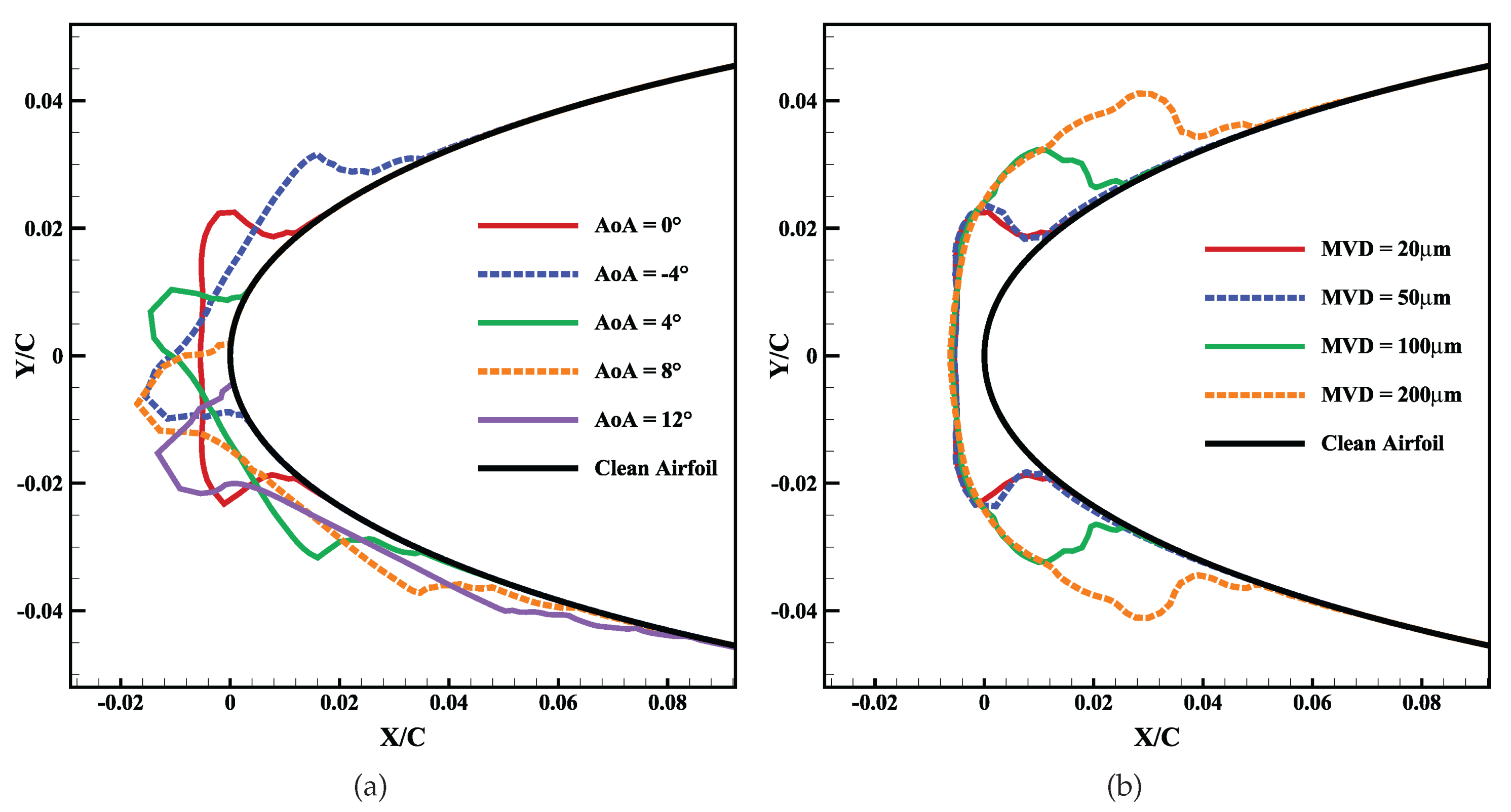
Figure 7.
Streamlines around the airfoil: (a) Clean airfoil; (b) Iced airfoil for case 1.
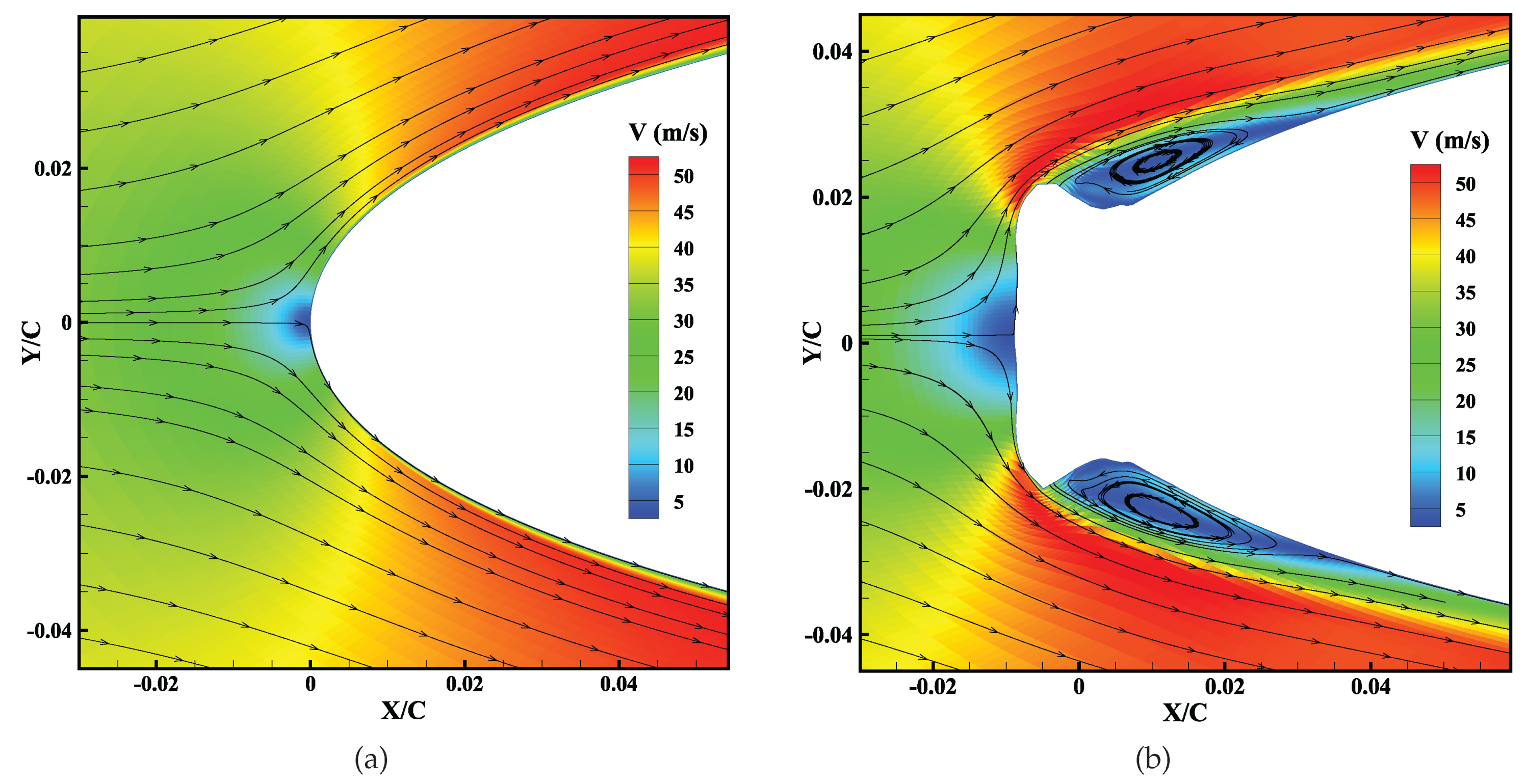
Figure 8.
Surface temperature distributions at different times in the de-icing process
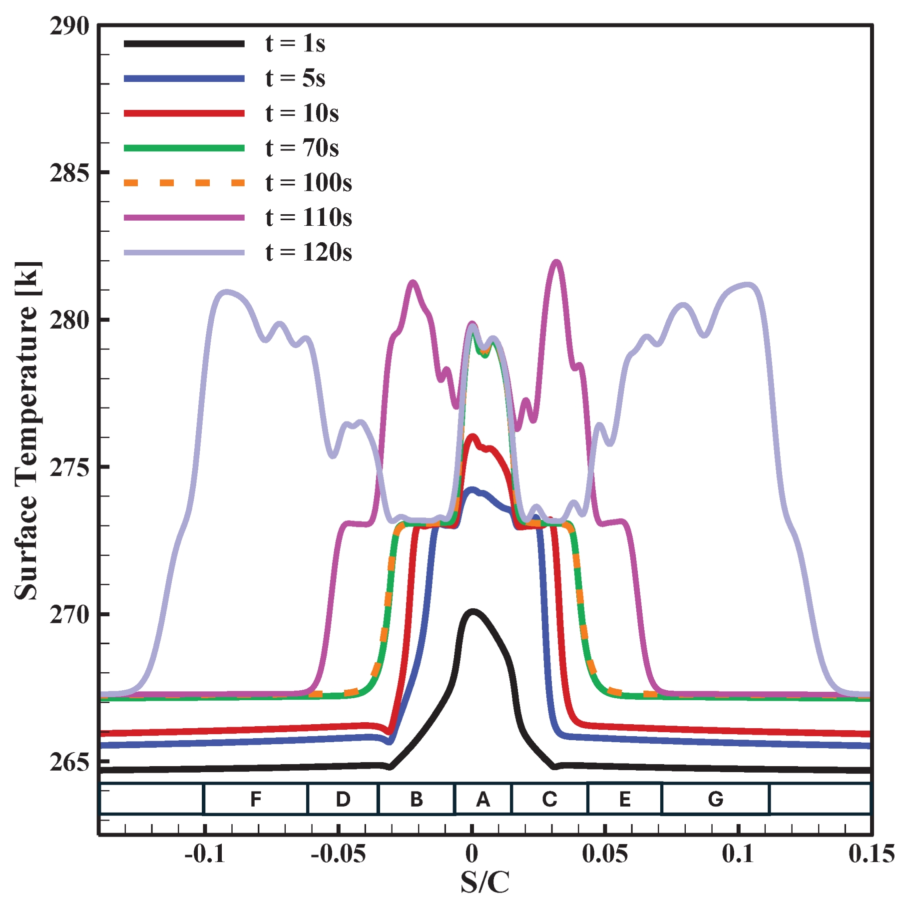
Table 1.
Computational Mesh Independence Evaluation.
| Computational | Total Number | First Cell | Drag Coefficient | Percentage Change |
|---|---|---|---|---|
| Grid | of Cells | Height [m] | (CD) | Compared to |
| Previous Mesh | ||||
| Coarse | 38,500 | 2.00E-06 | 0.01463 | - |
| Medium | 82,400 | 2.00E-06 | 0.01546 | 5.67% |
| Fine | 161,800 | 2.00E-06 | 0.01587 | 2.48% |
| Very Fine | 310,600 | 2.00E-06 | 0.01598 | 0.69% |
Table 2.
Properties of the ETIPS system [37].
Table 2.
Properties of the ETIPS system [37].
| Material | k [W/m.K] | [kg/] | [J/kg.K] | Thickness [mm] |
|---|---|---|---|---|
| Heating element (alloy 90) | 41.018 | 8906.26 | 385.112 | 0.0127 |
| Erosion shield (SS 301 HH) | 16.269 | 8025.25 | 502.32 | 0.2032 |
| Elastomer (COX 4300) | 0.256 | 1383.99 | 1255.8 | 0.2794 |
| Fiberglass/epoxy composite | 0.294 | 1794.07 | 1569.75 | 0.889 |
| Silicone foam insulation | 0.121 | 648.75 | 1130.22 | 3.429 |
Table 3.
Positions of the heating elements [37]
Table 3.
Positions of the heating elements [37]
| Heater | A | B | C | D | E | F | G |
|---|---|---|---|---|---|---|---|
| Start (S/C) | -0.0051 | -0.0329 | 0.0157 | -0.0607 | 0.0435 | -0.1024 | 0.0713 |
| End (S/C) | 0.0157 | -0.0051 | 0.0435 | -0.0329 | 0.0713 | -0.0607 | 0.1129 |
Table 4.
Power Density and duration of heaters
| Heating Element | Power Density [W/] | Duration [s] |
|---|---|---|
| A | 7750 | 0 to 120 |
| B-C | 15500 | 100 to 110 |
| D-E-F-G | 12400 | 110 to 120 |
Table 7.
Aerodynamic Coefficients degradation.
| Case | Change in | Change in | ||||
|---|---|---|---|---|---|---|
| Case 1 | 0 | 0 | - | 0.01587 | 0.01901 | 19.8% |
| Case 2 | -0.4109 | -0.3993 | -2.8% | 0.01706 | 0.02062 | 20.9% |
| Case 3 | 0.4108 | 0.4036 | -1.8% | 0.01705 | 0.02031 | 19.1% |
| Case 4 | 0.797 | 0.7837 | -1.7% | 0.02233 | 0.02558 | 14.6% |
| Case 5 | 1.104 | 0.9813 | -11.1% | 0.03656 | 0.05420 | 48.2% |
| Case 6 | 0 | 0 | - | 0.01587 | 0.01874 | 18.1% |
| Case 7 | 0 | 0 | - | 0.01587 | 0.02088 | 31.6% |
| Case 8 | 0 | 0 | - | 0.01587 | 0.02166 | 36.5% |
Disclaimer/Publisher’s Note: The statements, opinions and data contained in all publications are solely those of the individual author(s) and contributor(s) and not of MDPI and/or the editor(s). MDPI and/or the editor(s) disclaim responsibility for any injury to people or property resulting from any ideas, methods, instructions or products referred to in the content. |
© 2025 by the authors. Licensee MDPI, Basel, Switzerland. This article is an open access article distributed under the terms and conditions of the Creative Commons Attribution (CC BY) license (http://creativecommons.org/licenses/by/4.0/).
Copyright: This open access article is published under a Creative Commons CC BY 4.0 license, which permit the free download, distribution, and reuse, provided that the author and preprint are cited in any reuse.


