Submitted:
21 July 2025
Posted:
23 July 2025
You are already at the latest version
Abstract
Flapping wing micro aerial vehicles (MAVs), inspired by biological flight, offer advantages in acoustic stealth, aerodynamic efficiency, and mechanical resilience over rotary-wing platforms. This study presents the design, aerodynamic modeling, and fabrication of a bird-sized flapping-wing UAV. Employing empirical formulations from classical flight dynamics, structural and mechanical configurations were created with advanced design tools. Aerodynamic performance was predicted using quasi-steady blade element theory and advanced computational methods. Simulations confirmed that lift and thrust exceeded vehicle weight and drag, indicating viable sustained flight. The prototype was constructed using lightweight composite materials—carbon fiber for the fuselage and carbon rods with parachute fabric for wings and tail. A three-bar linkage mechanism converted motor input into oscillatory wing motion, with passive spanwise rotation optimizing the angle-of-attack throughout flapping cycles. Ground tests validated the aerodynamic predictions by demonstrating sufficient lift generation. This work provides a foundational platform for future research in bio-inspired MAVs, specifically targeting autonomous surveillance, lightweight propulsion, and low-speed maneuverability. Flutter analysis also identified a critical flutter velocity of approximately 415 m/s.
Keywords:
bio-inspired
; MAV
; blade element theory
; aerodynamic modeling
; prototyping
1. Introduction
Ornithopter is a flying object heavier than air that uses the concept of flapping of wings like birds. Duplicating a bird flight has been a human desire for many years due to high and efficient maneuverability and power saving abilities of these birds. The principle of flapping wings is the same to that of propeller-driven airplane [1]. However, the wings move up and down along with the forward motion in air. Near the body, the up and down movement is very small, however, as we move towards wingtip the amplitude of these motions increases. When wing moves downward, it slightly bends and the lift force vector makes an angle with the forward flight. This actually happens when a bird flies. In this case, the wing moves downward only, but the whole body moves upward along with the forward motion. In this way the bird generates large amount of thrust force without losing altitude. The wing is twisted such that to keep the angle of attack in position to maintain the altitude.
Figure 1.
Twist of wings and Production of Lift and Thrust.
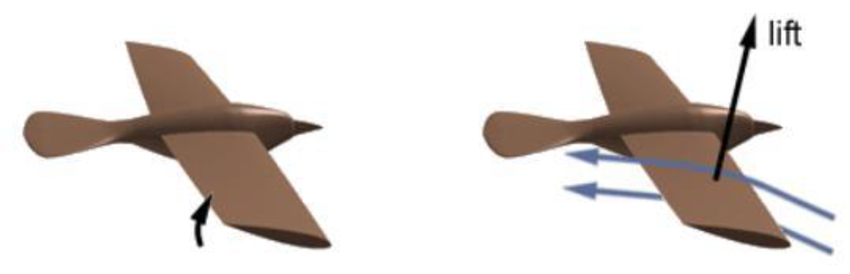
During upstroke, the angle of attack is reduced and the wing can pass through air with minimum resistance. At the same time, the bird folds the wing to decrease the wingspan, thus further reducing the drag. However, this particular capability is not necessary for all birds and ornithopters. Only the inner part of the wing produces lift during upstroke since there is a very small up and down motion near the body, however the magnitude is slightly small as compared to that produced during down stroke. This is the main reason why the body of bird slightly moves up and down during its flight [2].
Figure 2.
Production of Lift and Angle of Attack Adjustment.
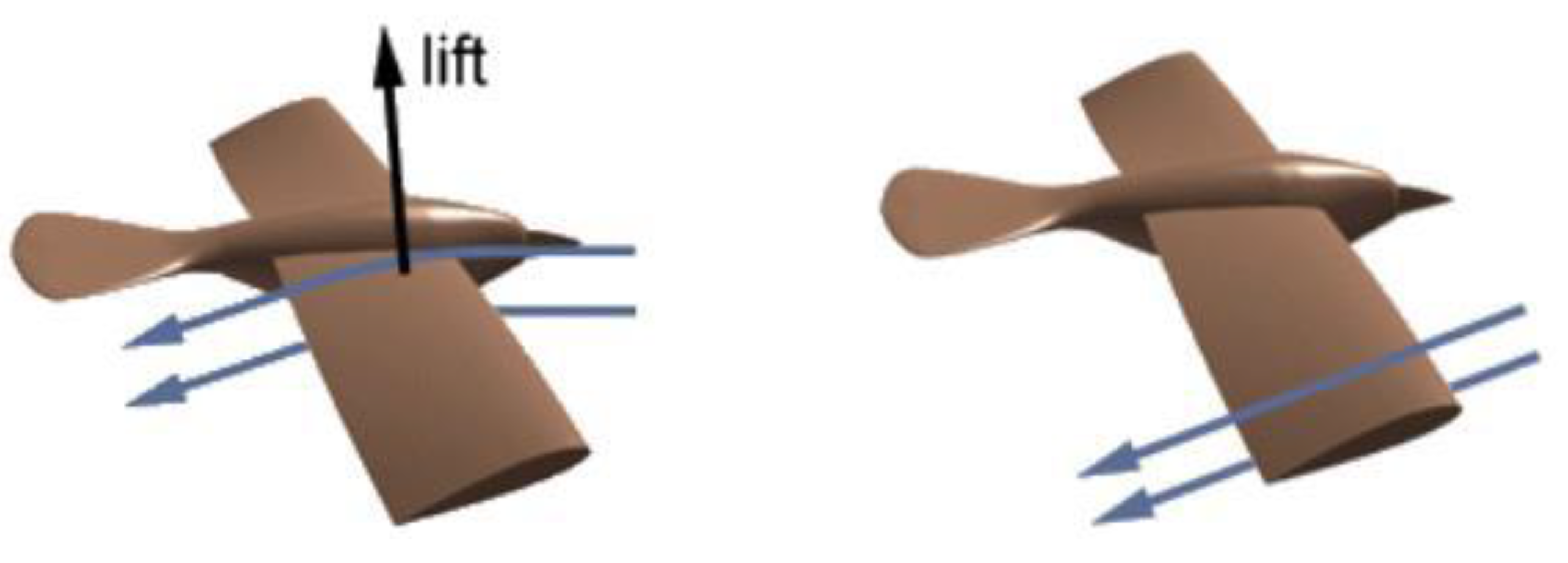
It is also observed from the bird flight that the outer portion of wing produces thrust and inner portion of the wing produces lift during bird flight. Development of these Flapping wing fliers (commonly known as Ornithopter) allows new mission requirements that are difficult or impossible for the large-sized aircrafts to accomplish. These micro vehicles are of special interest because of their use in many civil and military operations: Silent surveillance, buildings inspections, search and rescue missions and mapping. In addition to this these fliers can be equipped with various micro-sensors for microphones and cameras for remote areas detection. Flapping wing Micro Aerial Vehicles (MAVs) are useful for missions, which require more loitering times and longer mission ranges. Ornithopter provide highly versatile and maneuverable flight platform. Following objectives were achieved in this research:-
- Conceptual design of Ornithopter using empirical relations derived experimentally.
- Development of 3-D Model and the Actuation Mechanism with Simulation in CATIA
- Wing tips Kinematics
- Aerodynamics modeling & analysis of the Ornithopter using Modified Strip Theory.
- Fabrication of the modeled Ornithopter.
- Test Flight for successful completion of the project.
2. Literature Review
The early Ornithopters were developed for the manned flight. The initial work was carried out on the feathers that could be used to make wings for a man to fly and published in Chinese Book of Han in 19 AD [3]. Leonardo da Vinci, who studied the flight of birds for the first time and considered to be a pioneer in flapping wing flight, in order to imitate the bird flight, he sketched the design that could be used instead of the flying using the wings attached to the arms. No proper flapping flight was performed until 1929, in which the first successful manned flapping wing flight was achieved. Lippisch, a German engineer, was the first person to achieve the flight driven solely by the muscles of the pilot [4]. The flights were successful, but the Ornithopter did not have enough wing area, the bird could not fly for greater distance. Fig.2.3. shows the Lippisch manned Ornithopter flight.
After one-year Lippisch and his students manufactured many unmanned Ornithopters with power generated by engine. These were experimentally tested and the longest flight time obtained was 16 minutes. In 1942, Schmidt fabricated a small human-powered flapping wing Ornithopter capable of flying 900 meters at a constant height [5]. After 5 years, Schmidt built a double seater Ornithopter with the speed range of 100 to 120 kilometers per hour [6]. Figure 3 shows the Schmidt’s Ornithopter constructed in 1947 [6].
In 1993, DeLaurier constructed an ornithopter wing and tested it for flexibility to be used os a flappin wing [7] this wing was used in fabrication of an ornithopter subsequently as shown in Figure 4. DeLaurier gave a complex aerodynamics model for flapping wing aircraft which is still applicable on the micro-sized aircraft.
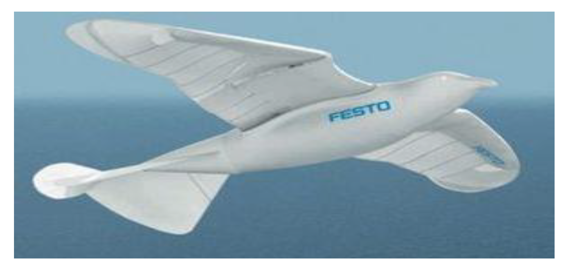
The bird sized aircrafts were started to be constructed during the era of Lippisch. Erich von Holst constructed rubber powered ornithopters and obtained greater efficiency. The model proposed by Eric resembled more closely to the natural birds [8]. In addition to this there are multiple of bird sized aircrafts available in the literature. In 1930, ornithopters were developed that were compressed air powered. These ornithopters, were bird like in shape and developed by Vincenz Chalupsky [9]. 1958, Percival Spencer manufacture bird shaped ornithopters driven by engines [10]. Sean Kinkade started a small-scale commercial production of remotely controlled ornithopter [8]. Some more designs were developed by several other engineers, that include RoboFalcon ornithopters specifically manufactured to chase the flock of birds [12] is remote controlled (RC) bird is commercially available for customers and foam made RC ornithopters close to the real bird were developed by Robert Musters in order to control the natural birds at airports [8]. Recently, Festo AG developed an ornithopter, named SmartBird with bending wing capabilities. The flier is controlled via radio and the motion of a seagull is imitated in the design. It only weighs 450 grams and its flight shows remarkable resemblance with nature [13].
Figure 5.
Festo Smart Bird [13].
Figure 5.
Festo Smart Bird [13].
Some micro ornithopters are capable of carrying camera as payload, thus allowing to be used as spy in buildings and remote areas. The idea is to obtain a flapping wing aircraft so small that it resembles the same to insects and small birds. In 1998, Aerovironment & Caltech developed the first micro aerial vehicle (MAV) ornithopter, named MicroBat [14]. It is of the size of a palm as shown in Figure 6. Till 2002, no hovering flight was achieved for a MAV ornithopter, when the first hovering ornithopter was developed at University of Toronto [15]. In 2006, scholars at the Technical University of Delft and Wageningen University developed Delfy, which is capable of forward and hovering transition during flight [16]. It is also equipped with small video camera thus giving the autonomous navigation ability to the ornithopter]. Nathan Chronister manufactured an ornithopter that can hover and perform quick maneuvers for recreational use in 2007. The size and weight of the ornithopter was same to that of real hummingbird, the smallest bird in the world [8]. However, the quest of miniaturizing wasn’t over yet. In the same year Petter Muren constructed the world’s smallest ornithopter, which was controlled via radio [17]. It has the span of 10 cm and weight of 1 gram only. Another huge breakthrough in the field of MAV was the development of Aerovironment’s Nano Hummingbird in 2010, because of its stabilized flight without any tail. The wing was allowed to rotate about 3 axes thus allowed maximum maneuverability capabilities [18].
For the successful flight of an aircraft, the initial design and analytical working is necessary. For this purpose, the important parameters & performance optimization techniques were studied. Experiments were performed using a motion-tracking technique on free-flying Drosophila to obtain three-dimensional wing trajectories. Similarly, Walker, Thomas, and Taylor [19] measured the complete wing trajectories of locusts and hoverflies in a low-speed closed-loop wind tunnel. The experiments were performed on three different desert locusts in order to obtain the important dynamics parameters [20]. Grätzel [21] also conducted experiments on Drosophila using a high-speed camera to capture the flapping motion of the wings. Zhang et al. [22] employed a Planar Single-Crank Double-Rocker mechanism, developed using ADAMS modeling software, to define the wing motion. Experiments by Ellington [23] and Ennos [24] demonstrated that wing motion follows a simple harmonic function. Harijono et al. [25] developed a kinematic and aerodynamic model by assuming the thin wing to be rigid and the motion to be three-dimensional. Benjamin Y. Leonard [26] divided the wing kinematics into three motions, that were rotation about each axis and considered the motion to be sinusoidal, however, with some offset and phase lag between the rotations as obtained experimentally. Another scholar, Bierling [27] assumed the fuselage of ornithopter to be rigid and the wings were attached at a single rotating joint that move with the required motion. Spline interpolation method was used to observe the wing kinematics data, which was further used to obtain the equations of motion of ornithopter. Whitney and R.J. Wood [28] performed passive-rotation flapping experiments artificial wings driven mathematically to measure the kinematics. This was further used to develop the blade-element aerodynamics model of the flapping wings. Jackson and Bhattacharya [29] derived the equations of motion of flapping using Eulerian Method. The central body was considered to be a point mass so that the hinges of both the wings was the same and placed at the central body. Two frames of references were used, one for each wing. This estimation eliminated the rotational motion of the central body.
The aerodynamic performance of a flapping wing aircraft cannot be completely defined by conventional aerodynamic theories due to the continuously varying flow field [30]. Scientists and biologists performed multiple of experiments to understand the flow phenomena around a flapping wing of natural bird. Many experiments were performed to obtain the effects of various parameters on the aerodynamics of already developed flapping wing aircrafts. As a result of these experiments many empirical relations and models for lift and thrust calculation have been generated, so that these models could be used effectively in analytical study of flapping motion. Analytical modelling for the aerodynamics of flapping wing can be categories into Quasi-steady and Unsteady aerodynamics. If the flapping frequency is low, quasi-steady approach can be applied as it ignores the wake effects and for high flapping frequency unsteady aerodynamics is used as it includes the wake effects.
The wing's complex structure also makes it difficult to understand the inertial forces and moments that play dominant role in determining the lift and thrust. Till now a number of attempts have been made to model the aerodynamics of flapping wing air vehicles. Hui Hu et al [31] performed experiments for aerodynamic performance of flexible membrane wings and discussed the flexibility effect of wings on aerodynamics. Similarly, Fry et al. [32] performed experiments on Drosophila and studied the kinematics and aerodynamics of bird. For this purpose, they used high speed infrared camera that was capable to capture kinematics for measuring the aerodynamic forces produced due to flapping.
There are several modeling techniques developed by many researchers and scholars, which may include blade element theory, momentum theory, lifting line theory and lifting surface theory, as classified by Smith et al [33]. Out of these theories, Blade element theory was implemented by DeLaurier [34] and Wei. Shy [35] in their ornithopter models. Dae-Kwan Kim et al [36] studied the aeroelastic analysis of a flexible flapping wing. The model used by them was modified strip theory with the high relative angle of attack and dynamic stall effects inclusion. Guji and Garcia [37] studied the distribution of forces on morphing wing aircrafts during the turning flight. Peters and his team [38] used the finite state model in order to obtain the aerodynamic forces and moments by improving the classical aerodynamics model of Theodersen [39].
Using the modified strip theory M.Y. Zakaria [40] developed an aerodynamics model and applied the model on commercially available Ornithopters previously done by the flyers considered in their study include SlowHawk 2 and Pterosaur Replica. In addition to these two biological flyers are also taken into account including Corvus monedula and Larus canus. These birds and ornithopters were previously studied by Daniel et al [41]. He investigated the aerodynamics parameters. Valiyff et al [42] performed wind tunnel testing on two commercially available ornithopters at low speed at different free stream velocities and flapping frequencies to verify the developed aerodynamics model based on blade element theory.
The final step in analytical modeling is the development of equations of motion of flapping wing aircraft. Very few engineers and scholars have worked to develop the control theory of ornithopter. Bierling [27], as described before considered the fuselage as rigid body with the wings attached a single joint and presented the complete flight dynamics model for an ornithopter with high flapping frequencies. The aerodynamics model used in the dynamics was the quasi-steady model developed by Fry et al. [32]. Similarly, Taylor et al. [19] examined the desert locust flight and established a fact that this motion confirms the rotary flight due to mass oscillations. Meirovitch [43] used a system of multi-bodies to obtain the equations of motion for an aircraft using the kinematics, structural parameters and aerodynamics of aircraft. Meirovitch obtained six degrees of freedom system and proposed the solution. Deng et al. [44] studied the motion of micro aerial flapping wing vehicles and developed the mathematical model of its motion. Focus was given to the difference between fixed wing and flapping wing dynamics. The analytically derived equations were then used to form the algorithms for body dynamics which was then introduced to the wing aerodynamics model, actuator dynamics and the environmental factors in order to make up Virtual Insect Flight Simulator (VIFS). Some engineers and scientists have worked on the hovering capabilities of an ornithopter and developed equations of motion. Faruque and Humbert [45] developed the longitudinal hovering dynamics of a flapping insect. Quasi-steady aerodynamics given by Fry et al. [32] was used with additional hovering parameters after considering the body to be rigid. In the similar manner they studied and developed the lateral equations of motion for the hover flight. The study was carried out for the longitudinal and lateral control of a flying insect. Jared Grauer et al. [46] used the visual tracking system and obtained the wing trajectory while the ornithopter under consideration was in straight and mean flight. Using the multi-body dynamics, they investigated the kinematics variables and system identification techniques to obtain the aerodynamics model equations of motion. Orlowski [47] derived the dynamics equations of a flapping wing aircraft by considering rigid wings attached to the rigid body. A study validating the use of 3D-printed aircraft models in subsonic wind tunnels confirmed that additive manufacturing can offer not only quick prototyping but also accurate performance replication [48]. This approach aligns with the modular and repairable design adopted in our bird-sized flapping wing aircraft, where interchangeable parts like wing spars and faceplates enhance field usability and adaptability. Manufacturing accuracy also plays a direct role in aerodynamic performance. An experimental investigation used point cloud and surface deviation analysis to evaluate discrepancies between the CAD model and actual wing surfaces [49]. Applying this methodology in ornithopter fabrication can ensure geometric precision in critical aerodynamic surfaces like wings and tail, improving lift symmetry and thrust uniformity during testing and flight.
Recent progress in machine learning and artificial intelligence has brought notable improvements to the field of aerodynamic design and optimization, especially for flapping-wing UAVs. Techniques like convolutional neural networks, generative adversarial networks, and reinforcement learning have enhanced turbulence prediction by approximately 20%, while also significantly cutting down the computational resources and time typically required by conventional CFD methods, which often struggle with capturing complex turbulent flows [50]. These AI-based methods support automated, multi-objective aerodynamic optimization, allowing for rapid refinement of wing shapes and motion patterns that are essential for efficient flapping flight. Furthermore, adaptive neural networks have proven highly effective in nonlinear aerodynamic challenges, including real-time shape optimization, drag minimization, and enhancing flight efficiency in both commercial and military aerospace applications. These networks help accelerate the design process, improve fuel economy, and increase overall system safety, indicating their strong potential to transform the design and operation of bio-inspired flapping wing UAVs [51].
3. Materials & Methods
The conceptual design of the ornithopter was developed based on initial design parameters using empirical relations proposed by Wei Shyy [35]. In addition to geometric parameters, key characteristics such as wingspan, mass, wing surface area, root chord, and flapping frequency were also determined [35]. After the series of experiments, effects of different parameters are studied on the flight characteristics [35]. Wing area, airspeed, density and wing loading are interconnected and are related as follows:
Span is approximated to be 1m and on the basis of the span further estimations are made.
| Mass: | m = (0.85×b) 2.56 |
| m = 0.66 kg | |
| Wing Area: | S = 0.16×m0.72 |
| S = .1186 m2 | |
| Root Chord: | c = (8×S)/(b×π) |
| c = .305 m | |
| Flapping Frequency: | f = 3.87×m−0.33; f = 4.439 Hz |
In summarized form these parameters are tabulated in Table 1.
The Kinkade’s Bird Hawk is selected for this study and proposed its geometric parameters as per the requirement. A detailed design of wing and tail are drawn on CATIA based on the proposed parameters that are given in Table 2.
The ornithopter is modeled on the software CATIA On the basis of geometric parameters CATIA design is made and is shown in Figure 7 This shows a rough sketch of the design according to the dimensions.
Fuselage is designed according to gear assembly diameter and the length of the ornithopter and is shown in Figure 8. Fuselage specifications are shown in Table 3.
Wings are the source of lift and thrust generation so they need to be designed to fulfill these criteria. Wings are designed in such a way that the central portion is stretched and tight whereas the outer portion is flexible. Primary, secondary and tertiary spars are arranged. Arrangement of tertiary spars is the critical part, which allows the flexion in the wing. For the visualization and to use it in the fabrication process the CATIA design is shown in Figure 9.

Table 4.
Wings Specifications.
| Parameters | Values |
|---|---|
| Span | 100 cm |
| Root Chord | 30.5 cm |
| Primary Spar | 50 cm |
| Sec. Spar | 46.16 cm |
| Area | 1186 cm2 |
| Aspect Ratio | 8.348 |
In order to obtain the required flapping frequency i.e., 4.43Hz the gear mechanism is designed with the gear reduction of 43:1. Design specifications of gears are mentioned in the Table 5.
Tail is designed as the 30% surface area as that of wing. Tail would be able to perform two maneuvers i.e., pitch and yaw. CATIA design of tail is shown in Table 6.
Figure 10.
(a) CAD Models of Gears; (b) CAD Model of Tail.

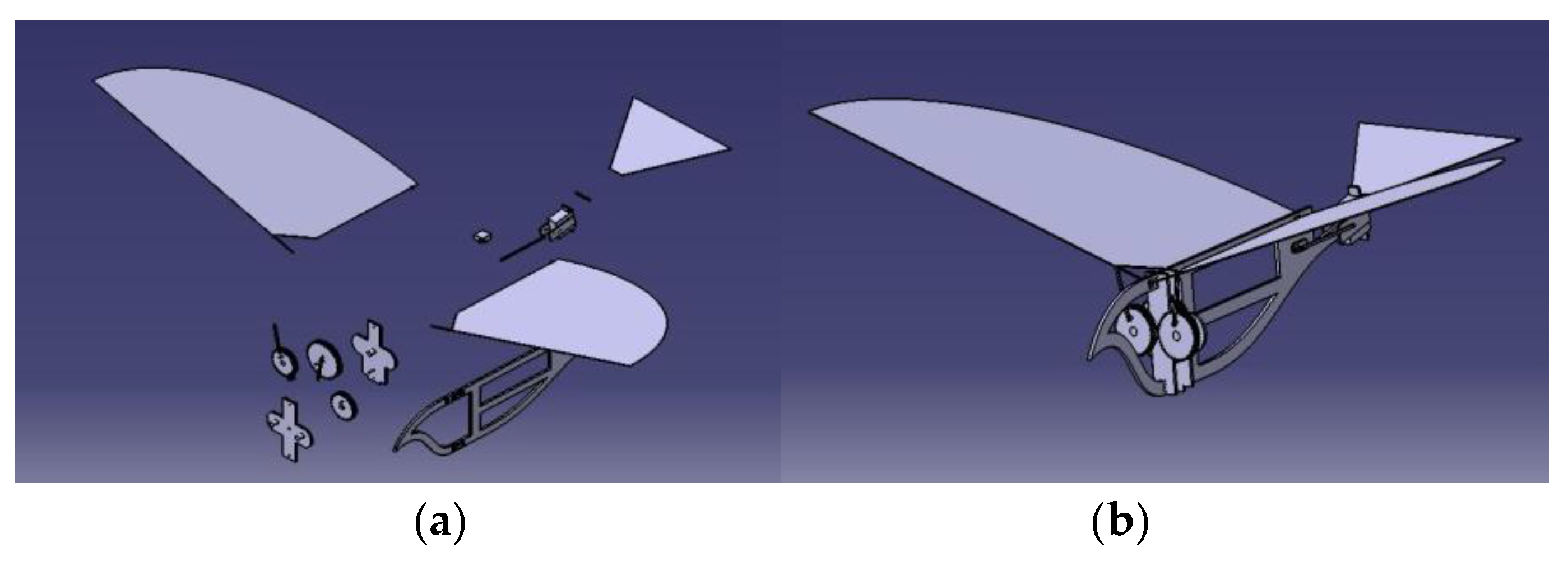
Assembly of bird sized aircraft is performed after designing of all individual parts in CATIA. This 3D model is then simulated to study its flapping mechanism.
Figure 11.
(a) Sub components of final assembly; (b) CAD Model of final assembly.
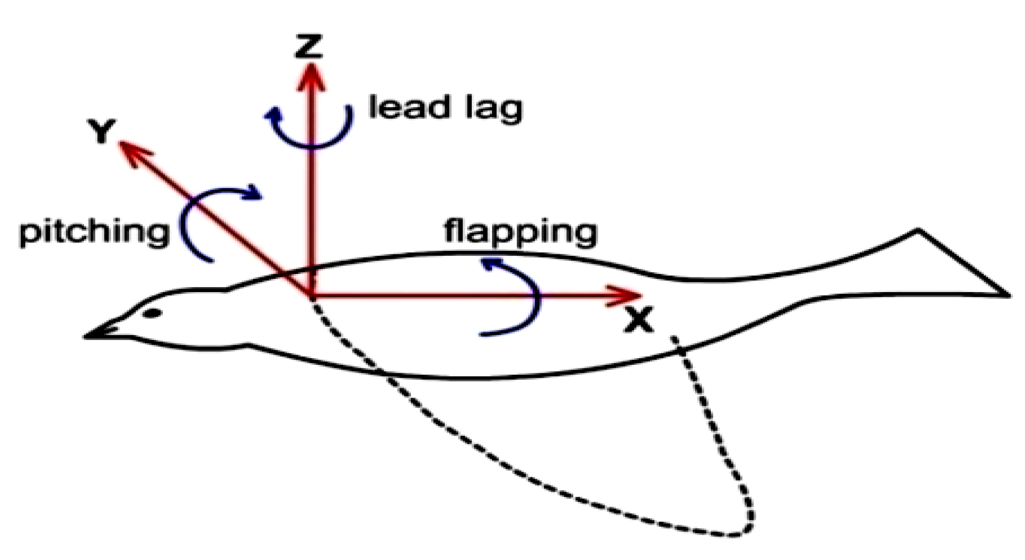
3.1. Kinematics of Flapping Wing & Analytical Modelling of Aerodynamics
The flapping wing motion of ornithopters and entomopters can generally be categorized into three classes based on wing kinematics and the mechanism of force generation: horizontal stroke plane, inclined stroke plane, and vertical stroke plane. One of the most distinctive features of insect flight is their unique wing kinematics]. Due to their smaller scale and biological design, insects fundamentally differ from birds. In insects, all actuation is performed at the wing root, while birds possess internal skeletons with muscle attachments that enable localized actuation along the wing—such as wing warping—although wing deflection in birds may also occur passively. As a result of these differing kinematic mechanisms, the aerodynamic characteristics of insect flight diverge significantly from those observed in fixed-wing, rotary-wing, or even bird flight. Based on Ellington’s study, the generic wing motion (using a semi-elliptical wing model) can be classified under the inclined stroke plane regime. In this case, the aerodynamic force generated during flapping can be decomposed into vertical and horizontal components—lift, thrust, and drag—across both upstroke and downstroke cycles. In contrast, the horizontal stroke plane produces a greater horizontal thrust component, while the vertical stroke plane, often observed during takeoff or hovering (e.g., butterflies), involves wing motion that is nearly perpendicular to the chord.
During flapping, the vertical component of induced airflow is maximal near the wing tips and diminishes toward the root. Consequently, for a constant forward speed, the relative angle of attack (AOA) decreases from tip to root. To maintain an attached flow at the tip and avoid excessive AOA, the wing must pitch in the direction of flapping. During the downstroke, the total aerodynamic force tilts forward, comprising both lift and thrust components. In the upstroke, the AOA is consistently positive near the root but can vary near the tip depending on the degree of pitching. If the AOA at the tip remains positive, the outer wing regions contribute to positive lift and drag. However, if the AOA becomes negative, they produce negative lift but positive thrust. In the present study’s kinematic modeling of flapping-wing flight in pterosaurs, only periodic flapping and pitching motions are considered. For simplification without loss of generality, the flapping axis is assumed to lie close to the body’s longitudinal axis, while the pitching axis is placed at the leading edge of the wing. Both the upstroke and downstroke motions are illustrated in Figure 12 which shows an inclined stroke plane characteristic of hovering flight in the long-eared bat (Plecotus auritus) [48].
The flapping wing motion consists of three main types:
- Flapping: The up-and-down motion generating the majority of the bird's power, with the largest degree of freedom.
- Feathering: The pitching motion along the wing span, adjusting the angle of attack for efficient flight.
- Lead-lag: The in-plane lateral movement of the wing, resulting from phase differences along the span, aiding in stability [38].
Figure 13.
Angular Movements of Wing.
Most of the practical ornithopters only employ flapping motion to generate lift and thrust with passive pitching caused by the aerodynamic and inertial loads because of flexible wings.
Analytical modelling for the aerodynamics of flapping wing is categorized into Quasi-steady and Unsteady aerodynamics [30]. If the flapping frequency is low, quasi-steady approach can be applied as it ignores the wake effects and for high flapping frequency unsteady aerodynamics is used as it includes the wake effects. The focus of this study was to improve the analytical solution while giving special attention to inertial forces, which plays a vital role in the generation of lift and thrust. Elastic bending moment equation is being used to calculate the inertial forces instead of Newtonian mechanics. Former includes both the elastic effects and material properties whereas later only uses the effect of mass to calculate inertial force. Aerodynamic forces are modeled using Blade Element Analysis (a quasi-steady approach), where the time-dependent problem is converted into a series of steady-state problems. Steady-state aerodynamics are used to calculate the forces. Due to the finite wingspan, unsteady wake effects reduce the net aerodynamic forces, which are accounted for using Theodorsen’s function [28]. The model simplifies by neglecting leading edge suction effects and other unsteady lift enhancement mechanisms, as they are minimal in ornithopters. This approach, however, is inadequate for simulating the highly unsteady flight of insects. In addition to aerodynamic forces, the inertial effects of airflow also contribute to the lift and thrust of FMAVs.
3.1.1. Assumptions
- The wings are made of a flexible membrane attached to a spar at the leading edge, with a half-elliptical wing shape.
- Only flapping is induced by the powertrain system, with equal up/down flapping angles.
- The front spar serves as a pivot for passive pitching movement, driven by aerodynamic and inertial loads.
- The flow is assumed to remain attached to the wing.
- Both flapping and pitching movements are modeled as sinusoidal functions, with a specified amount of lag.
- The upstroke and downstroke have equal durations.
Figure 14 illustrates the analytical model of the wing.
3.1.2. Kinematics
The wing flaps from top to bottom with total flapping angle of 2βmax as shown.
Figure 15.
Front view of Flapping Wings.

The flapping angle β varies as sinusoidal function. β and its rate are given by following equations
Here 0 is the maximum pitch angle, is the lag between pitching and flapping angle r is the distance along the span of the wing under consideration
The lag between pitching and flapping angle should be such that when the relative air velocity is maximum, the pitch angle should be maximum (fig. 5.3). It is possible only if the lag is 90o.
Figure 16.
Motion of flapping Wing in Side View.
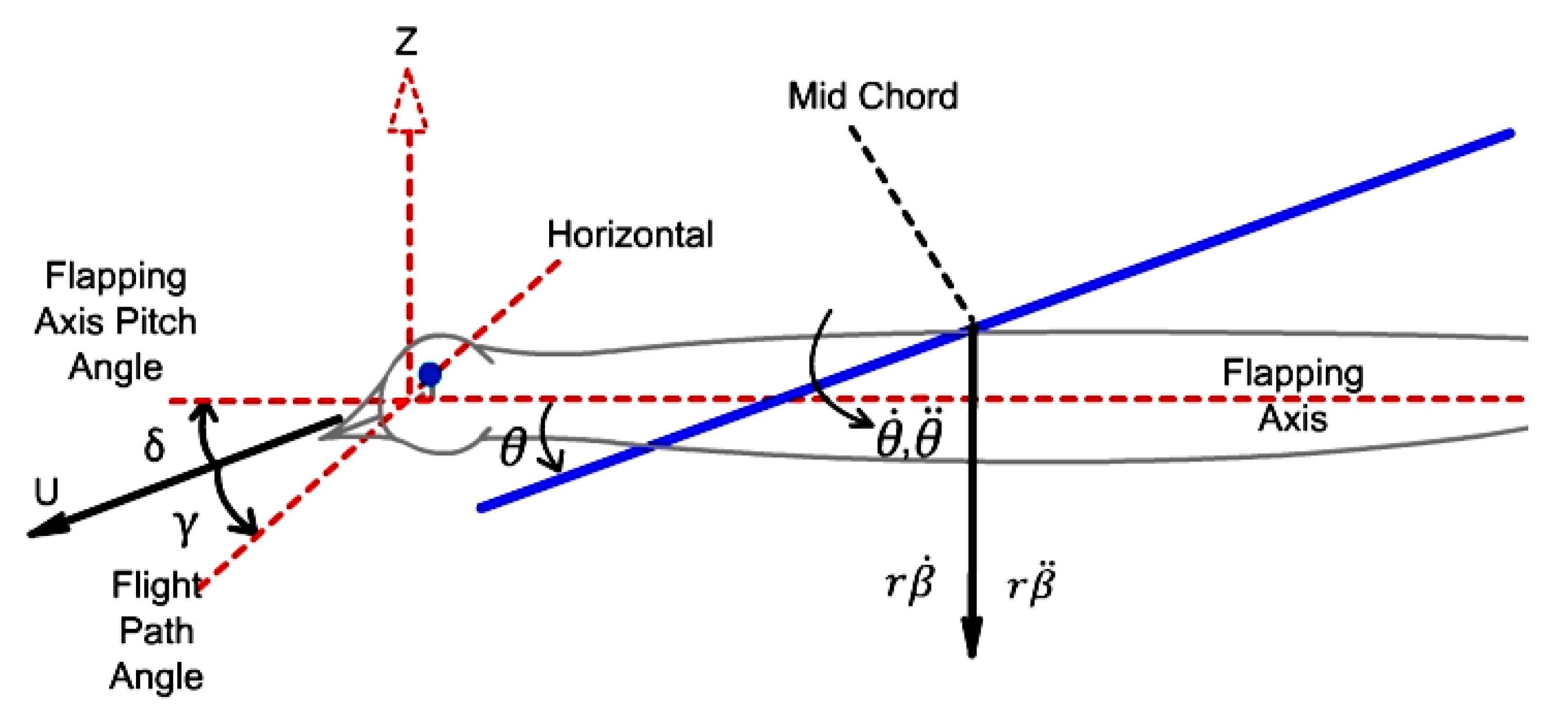
3.1.3. Modelling of Aerodynamic Forces
From Figure 17 we can find the vertical and horizontal components of relative wind velocity as under: -
For horizontal flight, the flight path angle γ is zero. Also 0.75c is the relative air effect of the pitching rate , which is manifested at 75% of the chord length [28].
Now we can find out the relative velocity, relative angle between the two velocity components ψ and the effective AOA as under:-
The section lift coefficient due to circulation (Kutta-Joukowski condition) for flat plate [28] is given by
where C(k) is the Theodorsen Lift Deficiency [17] factor which is a function of reduced frequency k and can be calculated as under
and are given by: -
The sectional lift dLc can be calculated as
Here c is the chord length and dr is width of the element of wing under consideration.
The apparent mass effect (momentum transferred by accelerating air to the wing) for the section, is perpendicular to the wing, and acts at mid chord [17], calculated by
The drag force has two components. These are calculated as:-
The total section drag is then given as
dDd = dDp + dDi
Figure 18.
Forces on Each Section of Wing.
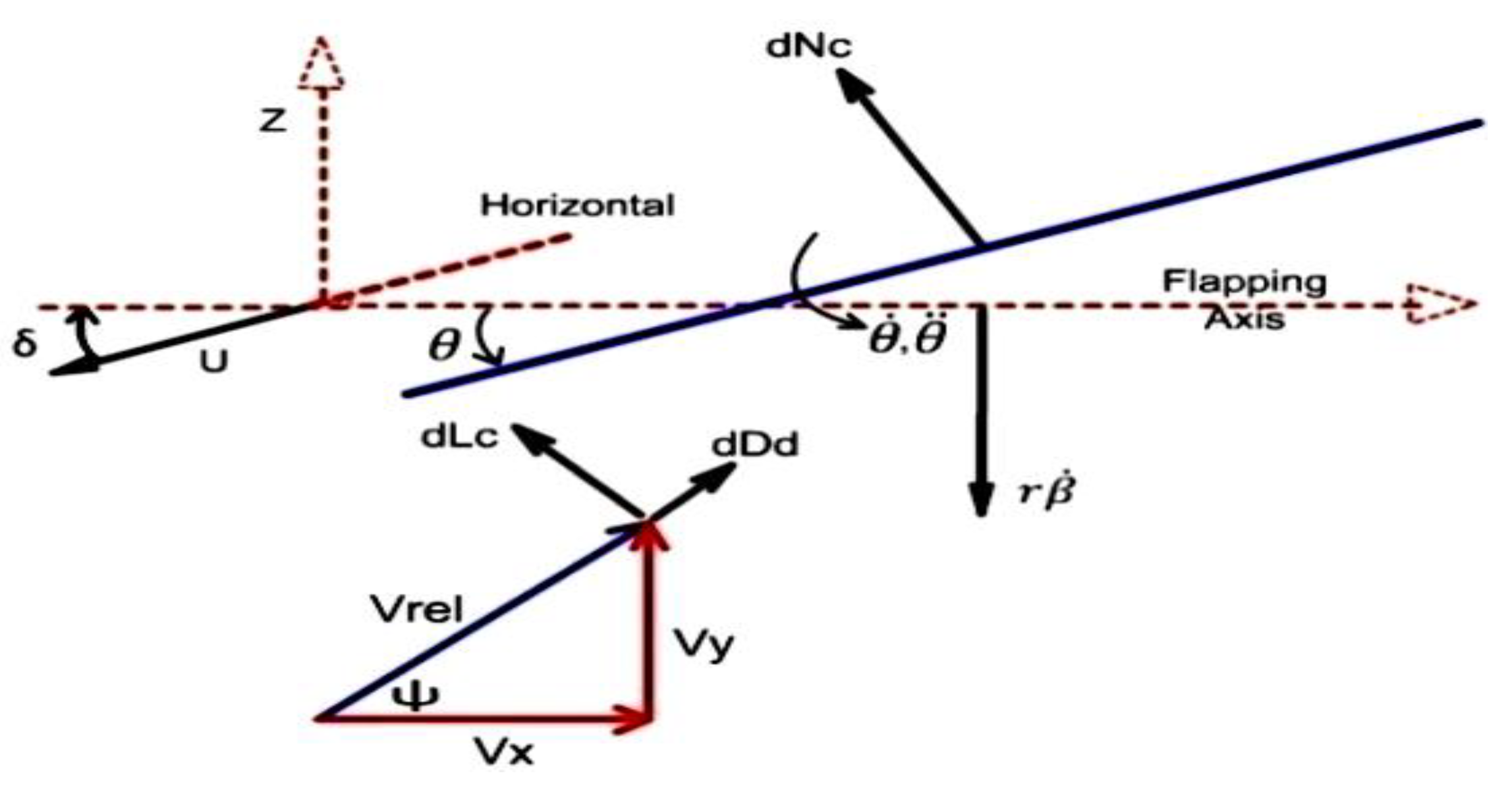
The circulatory lift dLc non-circulatory force dNnc and drag dDd for each wing section change direction at each instant during flapping. These forces are resolved into components perpendicular and parallel to the forward velocity in the vertical and horizontal directions, respectively. The vertical and horizontal components of the forces are given as:-
We can determine the lift and thrust of the ornithopter for each time instance. These forces are calculated for all time steps in one flap cycle, and the average values are taken to find the total average lift and thrust. If the wing is divided into ‘n’ strips of equal width and one flap cycle into ‘m’ equal time steps, then
Average lift =
Average Thrust =
Average Drag =
4. Results
A MATLAB script has been created to implement the analytical model, requiring 10 input parameters: the major and minor axes of the ornithopter wing, forward speed, flapping frequency, total flapping angle, fuselage incidence angle, maximum pitch angle, the lag between pitching and flapping, the number of spanwise strips, and the number of time steps in one flap cycle. The code performs the necessary calculations for all forces involved and presents the results in various graphical formats as needed.
Graphs for the Design Optimization
Before finding the aerodynamic forces, a MATLAB code is written in which the limits of the wingspan and the other factors were find out. The equations were taken from the papers and books. Few of the graphs are shown here in the Figure 19, Figure 20, Figure 21 and Figure 22.
Then a MATLAB code is written for finding the aerodynamic forces. Fig. 5.10 is showing the graph of the forces, which are generated during the flapping. The total lift (Blue), thrust (Green) and drag (Red) forces are shown in this graph. All the forces are in Newton. The fig. 5.10 also shows that the lift becomes negative, for some time, during up stroke but thrust and drag are not negative at most of the time. The parameters are flapping frequency of 4.44 Hz, total flapping angle 600, incidence angle of 50, pitching angle 200 , and lag of 900.
Figure 23.
All Forces Generate during Flapping.
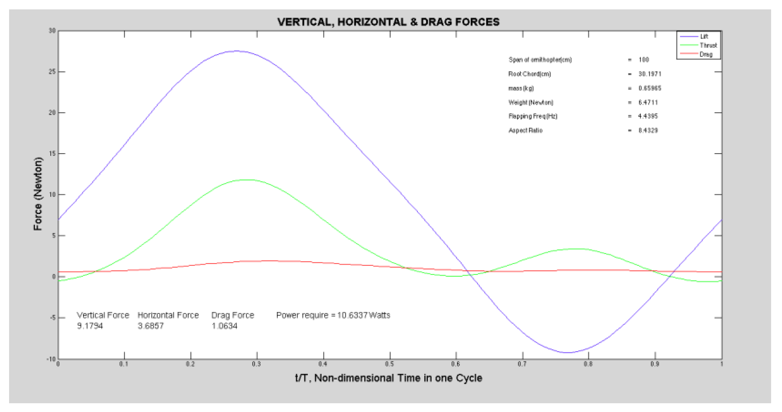
The above graph is giving us the results i.e., the forces in all the directions. The net results are showing that the lift is greater than the weight and the thrust is greater than the drag.
Then again, a MATLAB code is written for fing the leading-edge position of the wing during the cycle and the angles at which the forces are find out Figure 24 is showing the leading-edge position of the wing during the complete cycle. These are the angles at which the aerodynamic forces are calculated.
5. Discussion
The results was then compared with the Harijono Djojodihardjo et. al. [35]
From the above results it can be showed that the forces which are found out are having the same trends as in the Harijono et. a. and Harmons results.
It can be seen from the results that various flapping wing motion parameters influence the desired flight performance. The forward speed, flapping frequency, lag angle, angle of incidence, and total flapping angle are the key parameters. These factors once analyzed understand their impact on the flight characteristics and performance of the flight becomes clear. In this regard, there are numerous possibilities for varying the inputs and obtaining results in different forms, with a fixed wing size and geometry for the ornithopter the lift of the ornithopter is most influenced by the incidence angle and forward speed, while flapping frequency has the least impact. Thrust, on the other hand, is primarily affected by flapping frequency and forward speed, with incidence angle having the least influence. Additionally, the drag force increases as forward speed, incidence angle, and flapping frequency rise. Finally, an increase in the total flapping angle leads to an increase in all forces, but the most pronounced effect is seen on the drag force.
6. Fabrication of Flapping Wing Micro Unmanned Aerial Vehicle (MUAV)
Fabrication process is divided into seven major steps including assemblage of all the components to get the required product and testing of the aerial vehicle.
- Fabrication of Electronics
- Fabrication of Actuation Mechanism
- Fabrication of Fuselage
- Fabrication of Wings
- Fabrication of Tail
- Assembly of all components
- Testing
6.1. Fabrication of Electronics
While the electronics on the ornithopter are not critical to its mechanical function, they play a key role in defining one of the project's most important specifications: the minimum payload capacity. Since the rest of the ornithopter's sizing and design depend on this, the weight of the computer, interface equipment, sensors, and battery must be determined first. To drive the flapping mechanism, a high-torque motor is essential, and a brushless motor is chosen for this purpose. According to Ohm’s Law, the motor’s torque is inversely proportional to its resistance, while its RPM is directly proportional to the voltage, requiring a motor with low resistance. The most suitable motor available locally is selected, and its specifications are provided in Table 7. Motor is shown in Figure 27.
A three-cell lithium polymer (LiPo) battery was chosen due to its high energy and power-to-weight ratio, making it ideal for small, high-performance aerial systems. In the early stages of development, power density is prioritized over flight duration, as short test flights require brief but powerful bursts of energy. LiPo batteries can typically discharge at rates up to 10C, with some capable of 25C continuous discharge, providing the high output needed for flapping. Hence, a 3-cell LiPo pack was selected to meet the ornithopter’s power demands efficiently. Battery Specifications are given at Table 8. Battery is shown in Figure 28.
For the throttle control is used, the standard radios control airplane part i.e., electronic speed controller. Selected speed controller is of 30A as this indicates the upper limit of power required and the selected motor draws maximum current of 28A. Some more specifications of ESC are given in Table 9. Electronic Speed Controller is shown in Figure 29.
6.2. Fabrication of Actuation Mechanism
The drive mechanism is the most crucial part of the ornithopter, as it transforms the electric power from the battery into the flapping motion of the wings. Designing and fabricating this system is particularly challenging due to the need to withstand significant forces that change direction rapidly, while remaining both lightweight and durable. The actuation system includes the gear train and the linkage to the wing spars, which can be further separated into the gearbox and drive linkage components.
6.2.1. Gear Box
According to the requirements as described before the gears were designed and is shown in Figure 30.
In order to reduce weight of the gears, the holes on gears were made. Mounting provisions along with the shafts were machined and are made up of carbon fiber sheet and mild steel respectively. For the gear assembly first of the two plates were made on which the gears are to be fitted. A carbon fiber sheet was made and then from the IE Lab with the help of the carpenter the sheet that was very hard was cut into the desired shape with the help of the saw machine. After cutting the frame of the gearbox and aligning the gears shafts, complete gearbox is made. The test run of gearbox was then performed. Gear assembly was connected with the motor and speed controller and full battery was drained out in order to inspect any fault, but gearbox lived up to our specifications.
Figure 31.
Assembling of gears. (a) Gears and plates (b) Main gear assembled on the plate (c) Planetary gears assembled on the plate.
Figure 31.
Assembling of gears. (a) Gears and plates (b) Main gear assembled on the plate (c) Planetary gears assembled on the plate.
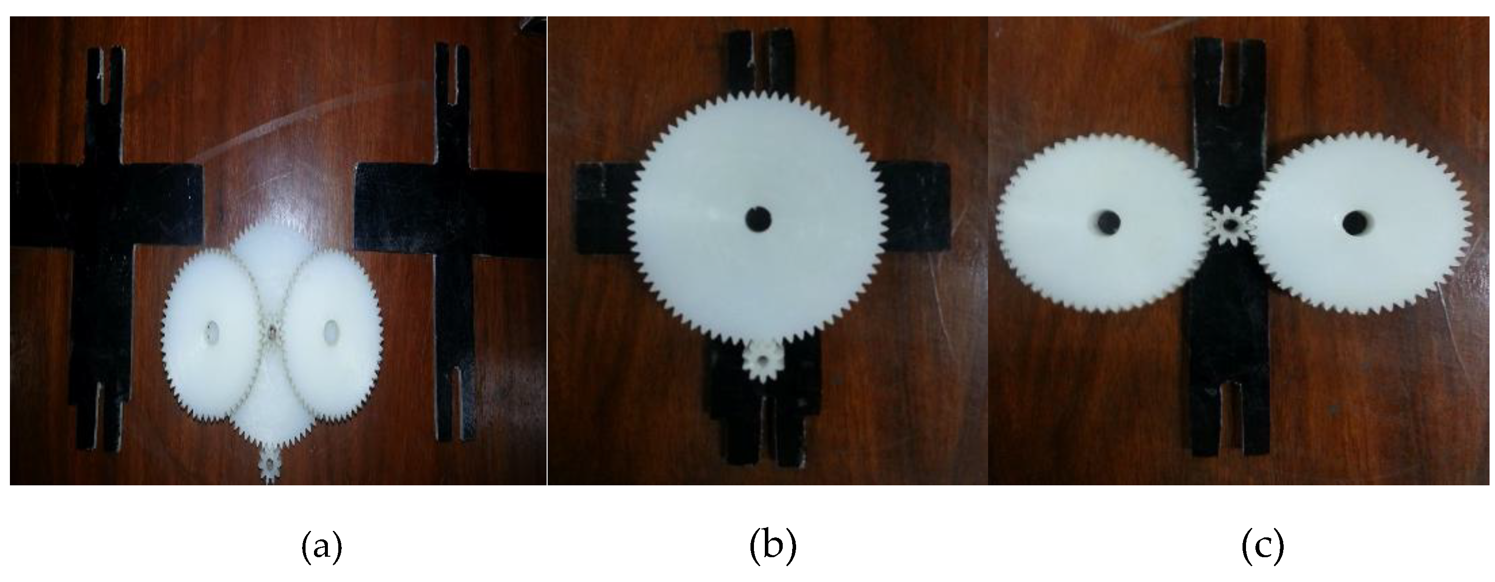
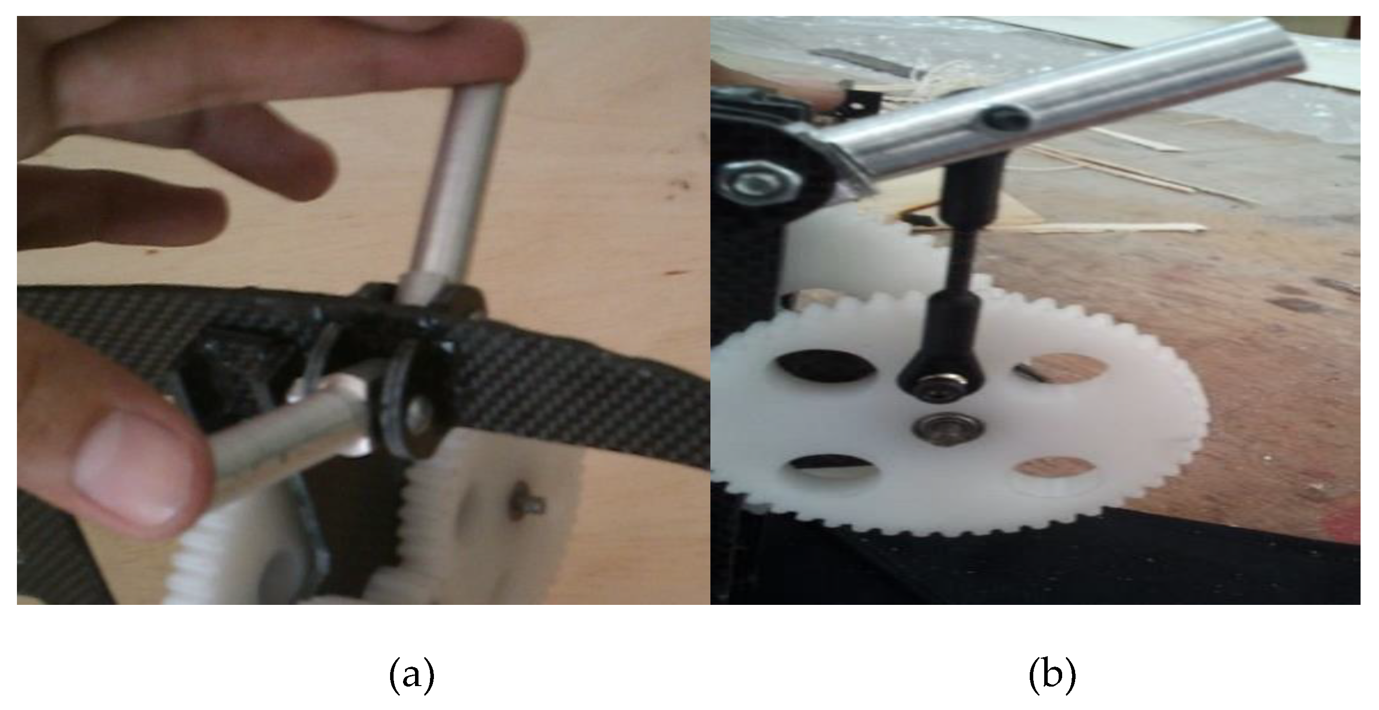
Figure 32 shows gears set mounted on fuselage subsequently.
6.2.2. Drive Linkage
To ensure the forces on the wings produce only thrust and lift, the wings must move in unison. This can be achieved with either a second, opposite four-bar linkage or a gear system that links the motion of one wing to the other. In this design, two separate linkages were chosen because the lightly loaded gearbox could be integrated directly into the ornithopter’s carbon fiber frame, making it easy to set up without interference. Given the small scale, lightweight materials were selected, as the linkages didn’t need to be overly strong. One challenge is that the crank and wing rotation occur on different axes, requiring additional degrees of freedom in the links to accommodate 3D motion. This was achieved using plastic ball joints, though they are prone to failure under load. The drive linkage consists of the connecting rod and wing connector. The connecting rod, made of mild steel with ball joints, links the gears to the wing spar and enables flapping. The wing connector, made of aluminum and ball bearings, links the wings to the fuselage. Since wing connectors were not available, they were custom-made in the IE Lab using a lathe. The connectors were carefully designed to balance strength and weight, ensuring they could withstand the load.
Figure 33.
Drive linkages. (a). Wing connectors; (b) Main drive linkage.
6.3. Fabrication of Fuselage
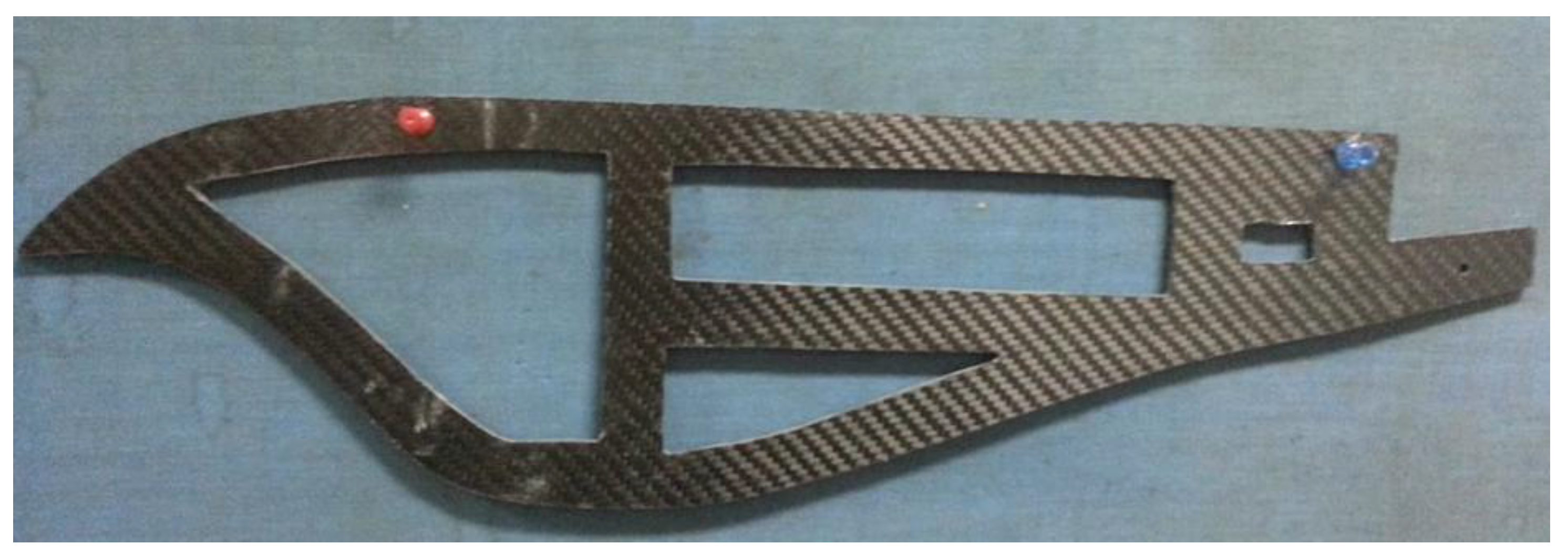
The fuselage of the ornithopter is relatively simple from a design perspective. Since the flapping mechanism is fully contained within the gearbox frame, the main frame primarily provides mounting points for the rear wing mounts, electronics, battery, and tail assembly. There are two design options for the frame: a single flat plate, which relies on its thickness for stiffness, or a three-dimensional structure made from thinner material that gains stiffness from a truss-like design. While the truss design would offer greater stiffness and lighter weight if needed, the frame doesn’t require significant stiffness in all directions. The rear wing mount helps prevent flexing in the direction where a flat plate would be weakest, as the wing spars form a large, stiff triangle. Thus, while the more complex structure might be stiffer and lighter, it offers little advantage in this case. The flat frame is much easier to design and fabricate and could even be lighter. Fuselage of ornithopter is fabricated from carbon fiber sheet due to its high strength and ability to damp out the vibrations. All the components like wing, tail and gearbox would be mounted on it so all the mounting provisions along with the body shape are firstly sketched in CATIA. The carbon fiber sheet was not available locally so it was imported from Greece. The sheet was cut using high precision CNC Machine.
Figure 34.
Fuselage.
6.4. Fabrication of Wings
For hovering flight the flapping of the wings are basically described by two movements.
As seen in the Figure 35 there is a horizontal motion indicated as up and down stroke.
The wings of the ornithopter also rotate around the span axis, which changes the angle of attack and allows for the generation of lift during both the upstroke and downstroke. The mechanism actively controls the horizontal motion, while the wing rotates passively around the pivot. The design of the wing ensures that the trailing edge creates a fanning motion to produce thrust, while the leading edge contributes to lift, alongside the lift generated by the airflow over the wing’s surface. The wing structure is made from carbon fiber tubes and covered with parachute cloth. One wing is shown in Figure 36.
6.4.1. Structure of Carbon Fiber Tube
The wings are supported by a triangular framework built from carbon rods. A primary spar runs along the leading edge, while a strut extends from the rear of the fuselage to a point near the spar’s tip. Several smaller rods branch out from this strut to the wing’s trailing edge and are allowed limited movement. This setup enables a fanning motion of the trailing edge that generates thrust, while the flapping motion of the leading edge contributes to both lift and the aerodynamic force from airflow over the wing.
6.4.2. Stitching of Parachute Cloth
The parachute cloth is stitched in such a way to form a cavity so that the spars pass through them. Firstly, the leading-edge cavity is mage in which the leading edge rod is placed and then after stretching the parachute cloth over the whole wing structure the parachute cloth is the stitched. Since stitching the cloth form pores and cavities hence disturbing the airflow so glue is put on the stitched part so cover the pores. Wing is shown in Figure 37.
6.4.3. Connection of Wings with Fuselage
The ends of the wing spars where the insertion occurs pose a significant engineering challenge, as this is the point where the driving torque is applied. Although the spar itself can withstand the torque, any attachment at the end to transfer the torque will create stress concentrations, which could lead to failure. Additionally, the spars must be designed for easy removal from the shoulder assembly, both for initial wing assembly and for replacement when damaged. To mitigate localized stress, the connectors are designed with a larger diameter. The wing's leading edge is positioned into these connectors, which are then attached to the fuselage, allowing for better load distribution along the spar’s length.
6.5. Fabrication of Tail
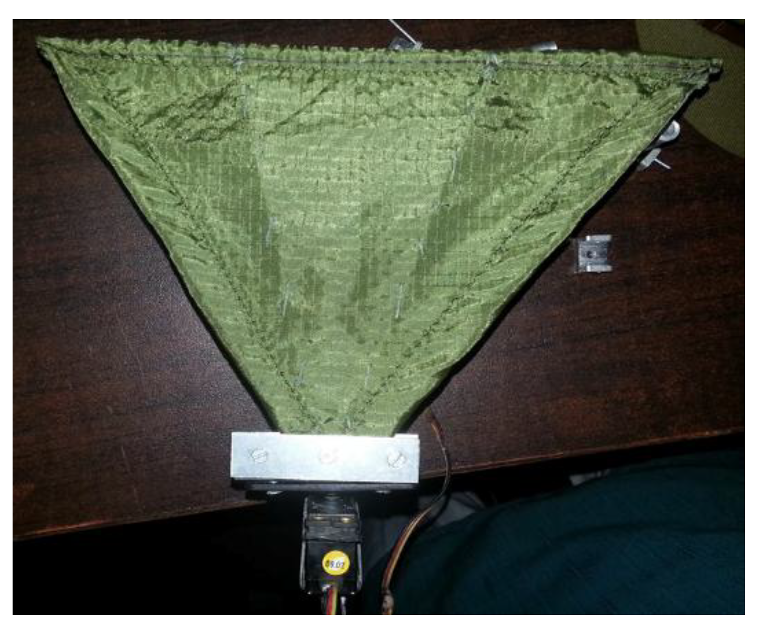
The tail is constructed in the same manner as the wings, utilizing carbon fiber rods and parachute cloth. It plays a dual role: providing pitch control and yaw control. In order to achieve two deflections of control surface two servo motors are used for elevator and rudder. The tail of the ornithopter controls the two primary degrees of freedom, along with the motor throttle. It features two servos: one directly connected to the tail at an angle, and another higher up on the body that moves the tail through a linkage. The rudder servo is angled to prevent unwanted vertical tail movement when adjusting the rudder. This setup allows the tail to stay in its trimmed position during horizontal flight, moving along a curved path independent of the elevator. While it doesn’t fully solve the issue of the elevator servo shifting the tail, it provides a significant control advantage.
6.5.1. Structure of Carbon Fiber Tubes
Firstly, same as for the wings a carbon fiber tubes structure is made and according to that structure parachute cloth is cut and pasted on the structure in order to make the tail.
6.5.2. Stitching of Parachute Cloth
After making the structure and cutting the parachute cloth the parachute cloth is pasted on the structure. The two cavities were made in which the rods are putted and the other rods were stitched and after stitching gluing was done to fill the pores made due to the stitching.
Figure 38.
Tail along with servos after complete fabrication process.
6.6. Assembly of All Components
6.7. Testing
The fabricated ornithopter was then tested in the AVDL (Aerospace vehicle design) Lab. Transmitter and receiver were issued from the AVDL Lab and tested there. The movement of the wings was noted and the joints and the linkages were checked. All the connectors and linkages were checked and all were right. There were no cracks in the joint and linkages. The position of the wing during the complete cycle and all the joints were right after testing the ornithopter, which shows the completion of the scope of the project.
7. Conclusion
This project involves the design, modeling, and fabrication of a bird-sized ornithopter, refined through minor changes to existing analytical models. The first phase covers concept selection, detailed design, and prototype construction using locally available materials. The gear train and wings were prioritized, as they are critical to the actuation and aerodynamic performance. In the second phase, body motion was analyzed using quasi-steady blade element theory through a custom MATLAB program, which estimated lift, thrust, and drag. Results showed sufficient lift and thrust for potential flight. Ground testing confirmed successful wing flapping and tail movement, validating the mechanical design. The ornithopter was built for research, with lightweight, repairable parts like modular spars and faceplates. Though designed at bird-scale, the concept can be adapted for micro aerial vehicles and further enhanced with autopilot systems for surveillance applications.
Author Contributions
Conceptualization, Sheharyar Nasir. and Kamran Hashmi.; methodology, Sheharyar Nasir; software, Kamran Hashmi.; validation, Sheharyar Nasir and Kamran Hashmi.; formal analysis, Kamran Hashmi; investigation, Kamran Hashmi.; resources, Kamran Hashmi.; data curation, Sheharyar Nasir.; writing—original draft preparation, Kamran Hashmi.; writing—review and editing, Sheharyar Nasir.; visualization, Kamran Hashmi.; supervision, Sheharyar Nasir;. All authors have read and agreed to the published version of the manuscript.
Funding
This research received no external funding.
Data Availability Statement
The data presented in this study are available upon request from the corresponding author. The data is not publicly available due to ongoing research and development activities associated with the presented prototype.
Acknowledgments
The authors have reviewed and edited the output and take full responsibility for the content of this publication.”
Conflicts of Interest
The authors declare no conflicts of interest. The funders had no role in the design of the study; in the collection, analyses, or interpretation of data; in the writing of the manuscript; or in the decision to publish the results.
References
- Qiuhong, Li, He Jiandong, Wu Chong, Cui Yuan, and Zhang Bokai. "Study on the Aerodynamic Characteristics of Bird-like Flapping Wings Under Multi-degree-of-Freedom Conditions." International Journal of Aeronautical and Space Sciences (2025): 1-9. [CrossRef]
- Fang X, Wen Y, Gao Z et al (2023) Review of the flight control method of a bird-like flapping-wing air vehicle. Micromachines (Basel) 14:1547. [CrossRef]
- Laufer, Berthold. The Prehistory of Aviation. United States: Field Museum of Natural History, 1928. ISSBN: 9780608021140, 0608021148.
- Lippisch, Alexander M. "Man powered flight in 1929." The Aeronautical Journal 64, no. 595 (1960): 395-398. [CrossRef]
- Lange, Bruno, ‘Typenhandbuch der deutschen Luftahrttechnik’, Koblenz, 1986. ISBN-13: 9783763752843 [Available Online]: https://www.booklooker.de/Bücher/Bruno-Lange+Typenhandbuch-der-deutschen-Luftfahrttechnik/id/A02G9y7E01ZZt?zid=en26cpd3te6294aighk3grkuvi.
- Human Powered Ornithopter Flight In Flapping Wings’, Newsletter, Fall 2010, [Available Online] : www.ornithopter.org.
- DeLaurier JD. The development of an efficient ornithopter wing. The Aeronautical Journal. 1993;97(965):153-162. [CrossRef]
- Chronister, Nathan. "The Ornithopter Design Manual." Published by the Ornithopter Zone, (2008). https://www.ornithopter.org/archive/ODM5.pdf.
- Flugsport, ‘Ornithopters of Vincenz Chalupsky powered by compressed air’, article no. 7, Page no. 191, 1937.
- Goodheart, Benjamin J. "Tracing the history of the ornithopter: past, present, and future." Journal of Aviation/Aerospace Education & Research 21, no. 1 (2011): 31-44. [CrossRef]
- Full History of Ornithopters, Ornithopter Society . Available at: https://ornithopter.org/history.full.shtml.
- Chen, Ang & Song, Bifeng & Wang, Zhihe & Xue, Dong & Liu, Kang. (2022). A Novel Actuation Strategy for an Agile Bioinspired FWAV Performing a Morphing-Coupled Wingbeat Pattern. IEEE Transactions on Robotics. PP. 1-18. [CrossRef]
- Festo Corporate, SmartBird – bird flight deciphered, 2012. Available Online: https://www.festo.com/us/en/e/about-festo/research-and-development/bionic-learning-network/bionic-flying-objects/smartbird-id_33686.
- Pornsin-Sirirak, T. & Tai, Yu-Chong & Ho, Chih-Ming & Keennon, Matt. (2001). Microbat: A Palm-Sized Electrically Powered Ornithopter. Proceedings of NASA/JPL Workshop on Biomorphic Robotics. Available Online: https://www.researchgate.net/publication/254717311_Microbat_A_Palm-Sized_Electrically_Powered_Ornithopter.
- Nick Pornsin-Sirirakm, Yu-Chong Tai, Chih-Ming Ho and Matt Keennon, ‘Microbat: A Palm-Sized Electrically Powered Ornithopter’, Proc. NASA/JPL Workshop on Biomorphic Robotics, pp. 14-17, 200.
- de Wagter, C 2022, 'Hover and fast flight of minimum-mass mission-capable flying robots', Doctor of Philosophy, Delft University of Technology. [CrossRef]
- T. Robyn Lynn Harmon, ‘Aerodynamic Modeling of a Flapping Membrane Wing using Motion Tracking Experiments’, Masters thesis, Faculty of the Graduate School of the University of Maryland, College Park, ProQuest, 2008.
- BBC news, ‘Hummingbird robot revealed in US’, 19 February 2011. https://www.bbc.co.uk/news/world-us-canada-12513315.
- G. K. Taylor, R. J. Bomphrey, and J. Hoen, ‘Insect Flight Dynamics and Control’, AIAA Aerospace Sciences Meeting and Exhibit, 2006.
- Walker, S. M. Thomas, A. L. R. and Tayler, ‘Photogrammetric reconstruction of high-resolution surface topographies and deformable wing kinematics of tethered locusts and free-flying hoverflies’, J. R. Soc. Interface 6, University of Oxford, UK, 2009.
- Graetzel, C. F Fry, S. N. Beyeller, F. Sun Y and Nelson, ‘Real-time microforce sensors and high speed vision system for insect flight control analysis’, Experimental Robotics: The 10th International Symposium on Experiment Robotics, 2008.
- Tao Zhang, Chaoying Zhou, Xingwei Zhang and Chao Wang, ‘Design, Analysis, Optimization and Fabrication of A Flapping Wing MAV’, International Conference on Mechatronic Science, Electric Engineering and Computer, Jilin, China, August 19-22, 2011.
- Ellington CP,‘The Aerodynamics of hovering insect flight’, Phil. Trans. Of Roy. Soc. London, Bio.Sci, Vol. 35, Feb 1984.
- Ennos AR,‘Wing Kinematics and aerodynamics of the free flight of some Diptera’, Journal of Experimental Biology, vol. 142, pp. 49-85, 1989.
- Harijono Djojodihardjoa, Alif Syamim Syazwan Ramli and Surjatin, ‘Kinematic and Aerodynamic Modelling of Flapping Wing Ornithopter’, International Conference on Advances Science and Contemporary Engineering, 2010.
- Benjamin Y. Leonard, ‘Flapping Wing Flight Dynamic Modeling’, Masters of Science thesis, Faculty of the Virginia Polytechnic Institute and State University, 2011.
- Bierling, and Patil,‘Nonlinear Dynamics and Stability of Flapping-wing Flight’, International Forum on Aeroelasticity and Structural Dynamics, 2009.
- J.P. Whitney and R.J. Wood, ‘Aeromechanics of passive rotation in flapping flight’, Journal of Fluid Mech., vol. 660, pp. 197-220, 2010.
- J. Jackson, R. Bhattacharya and T. Strganac, ‘Modelling and suboptimal trajectory generation for a symmetric flapping wing vehicle’, Proceedings of the AIAA Guidance, Navigation and Control Conference and Exhibit, Honolulu, Hawaii, USA, 2008.
- Ellington CP, ‘The aerodynamics of hovering insect flight. I. The quasi-stead analysis’, Philosophical Transactions of the Royal Society of London. Series B, Biological Sciences, vol. 305, issue 1122, pp. 1-15, 1984.
- Hui Hu, Anand Gopa Kumar, ‘An Experimental Study of Flexible Membrane Wings in Flapping Flight’, 46th AIAA Aerospace Sciences Meeting and Exhibit, Orlando, Florida, Jan 2008.
- S.N. Fry, R. Sayaman and M.H. Dickinson, ‘The Aerodynamics of Free-flight Maneuvers in Drosophila’, Science, Vol. 300, April 2003.
- M. J. Smith, P.J. Wilkin, M. H. Williams, ‘The advantages of an unsteady panel method in modelling the aerodynamic forces on rigid flapping wings’, The Journal of Experimental Biology, Vol. 199, 1996.
- J.D. DeLaurier, ‘An Aerodynamic Model for Flapping Wing Flight’, The Aeronautical Journal of the Royal Aeronautical Society, April 1993.
- Wei Shyy, Yongsheng Lian, Jian Tang Dragos Vilieru, Hao Lu, ‘Aerodynamics of Low Reynolds Number Flyers’, CAMBRIDGE University Press, New York, United States, 2008.
- Dae-Kwan Kim, Jun-Seong Lee, Jin-Young Lee and Jae-Hung Han, ‘An Aeroelastic Analysis of a Flexible Flapping Wing Using Modified Strip Theory’, SPIE 15th Annual Symposium Smart Structures and Materials, vol. 6928, 2008.
- E. Cuji. And E. Garcia, ‘Prediction of aircraft dynamics with shape changing wings’, Active and Passive Smart Structures and Integrated Systems, edited by M. Ahmadian, Proc. Of SPIE, United States, 2008.
- D.A. Peter, S. Karunamoorthy and W.M. Cao, ‘Finite state induced flow models part I: Two-dimensional thin airfoil’, Journal of Aircraft, Vol. 32, 1995.
- T. Theodersen, ‘General theory of aerodynamic instability and the mechanism of flutter’, Technical report, NACA Report 496, 1935.
- M.Y. Zakaria, A.M. Elshabka, A.M. Bayoumy, O.E. Abd Elhamid, ‘Numerical Aerodynamic Characteristics of Flapping Wings’, 13th International Conference of Aerospace Sciences and Aviation Technology, May 26-28, 2009.
- Ramji Kamakoti, Mats Berg, Daniel Ljungqvist and Wei Shyy, ‘A Computational Study of Biological Flapping Wing Flight’, Transactions of the Aeronautical Society of the Republic of China, Vol. 32, 2000.
- A. Valiyff, J. R. Harvey, M. B. Jones, S. M. Henbest, and J. L. Palmer, ‘Analysis of Ornithopter-Wing Aerodynamics’, 17th Australian Fluid Mechanics Conference, Auckland, New Zealand, 5-9 December, 2010.
- L. Meirovitch, ‘Methods of Analytical Dynamics’, McGraw-Hill Book Company, New York, 1970.
- X. Deng, L. Schenato, W. C. Wu and S. S. Sastry, ‘Flapping Flight for Biomimetic Robotic Insects: Insects: Part I – System Modeling’, IEEE Transaction on Robotics, Vol. 22, August 2006.
- I. Faruque and J. S. Humbert, ‘Dipteran insect flight dynamics. Part I: Longitudinal motion about hover’, Journal of Theoretical Biology, Vol. 64, May 2010.
- Jared Grauer, Evan Ulrich, James Hubbard Jr., James Hubbard, Darryll Pines, and J. Sean Humbert, ‘Testing and System Identification of an Ornithopter in Longitudinal Flight’, Journal of Aircraft, Vol. 48, March-April, 2011.
- C. Orlowski, A. Girard, and W. Shyy, ‘Derivation and Simulation of the nonlinear dynamics of flapping wing micro-air vehicle’, Progress in Aerospace Sciences, 2012.
- Raza, A., Farhan, S., Nasir, S., & Salamat, S. (2021, January). Applicability of 3D printed fighter aircraft model for subsonic wind tunnel. In 2021 International Bhurban Conference on Applied Sciences and Technologies (IBCAST) (pp. 730-735). IEEE.
- Ahmad, M., Nasir, S., ur Rahman, Z., Salamat, S., Sajjad, U., & Raza, A. (2021). Experimental Investigation of Wing Accuracy Quantification using Point Cloud and Surface Deviation. Pakistan Journal of Engineering and Technology, 4(2), 13-20.
- Sahibzada, S., Malik, F. S., Nasir, S., & Lodhi, S. K. (2025). AI-Augmented Turbulence and Aerodynamic Modelling: Accelerating High-Fidelity CFD Simulations with Physics-informed Neural Networks. International Journal of Innovative Research in Computer Science and Technology, 13(1), 91-97.
- Sahibzada, S., Malik, F. S., Nasir, S., & Lodhi, S. K. (2025). Generative AI Driven Aerodynamic Shape Optimization: A Neural Network-Based Framework for Enhancing Performance and Efficiency. International Journal of Innovative Research in Computer Science and Technology, 13(1), 98-105.
- Norberg, U.M., ‘Hovering Flight of Plecotus auritus’, L. Bijdr. Dierk 40, 62-66 (Proc.2nd int. Bat.Res, Conf.), 1970.
Figure 3.
Schmidt’s Human-Powered Ornithopter.
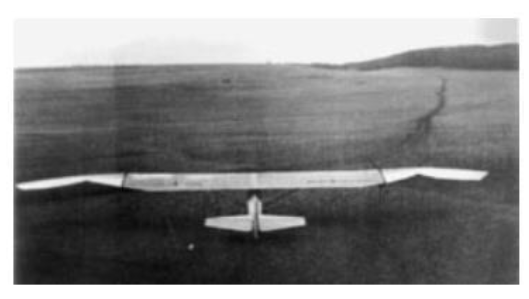
Figure 4.
James DeLaurier’s Ornithopter.
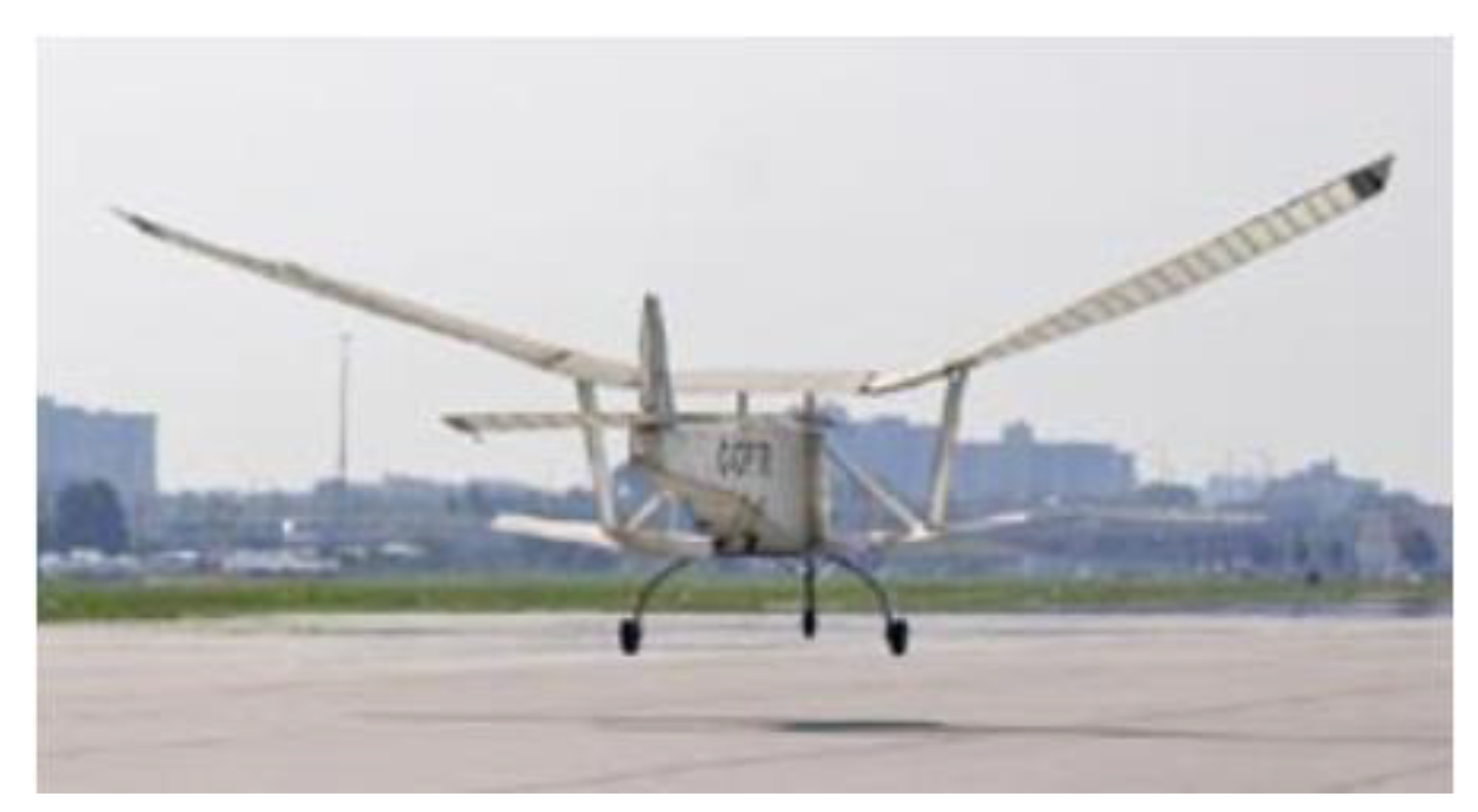
Figure 6.
Micro Air Vehicles Ornithopters developed recently.
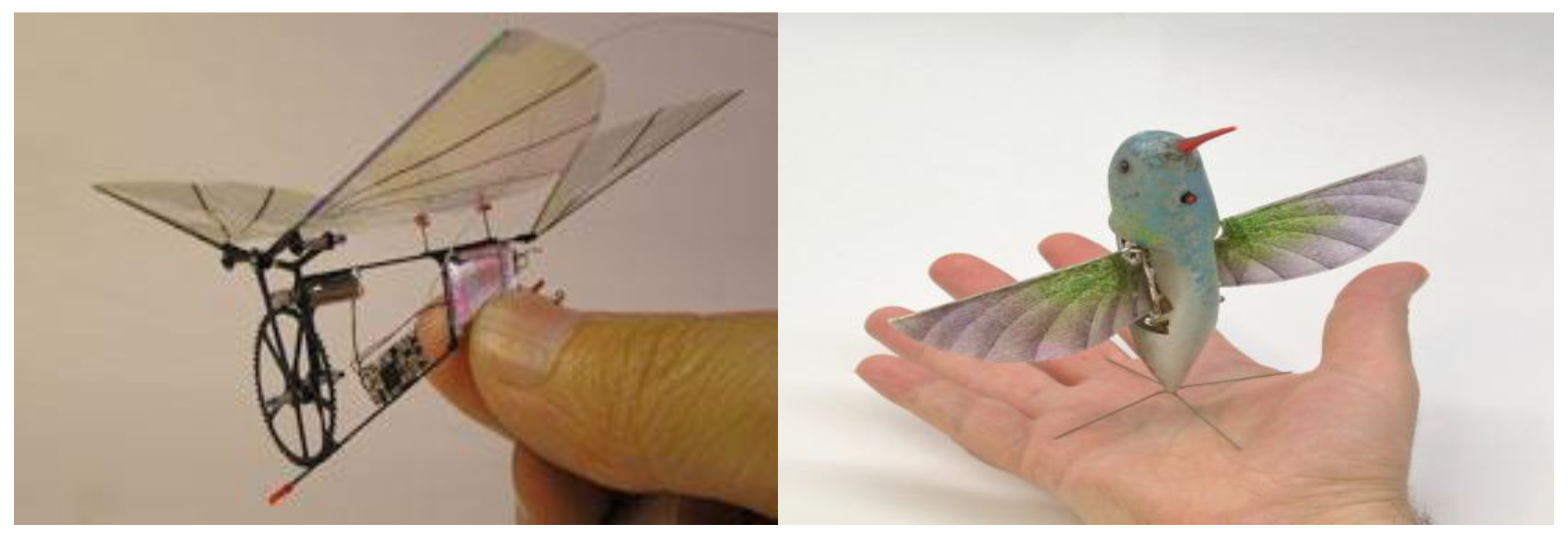
Figure 7.
Basic Sketch.
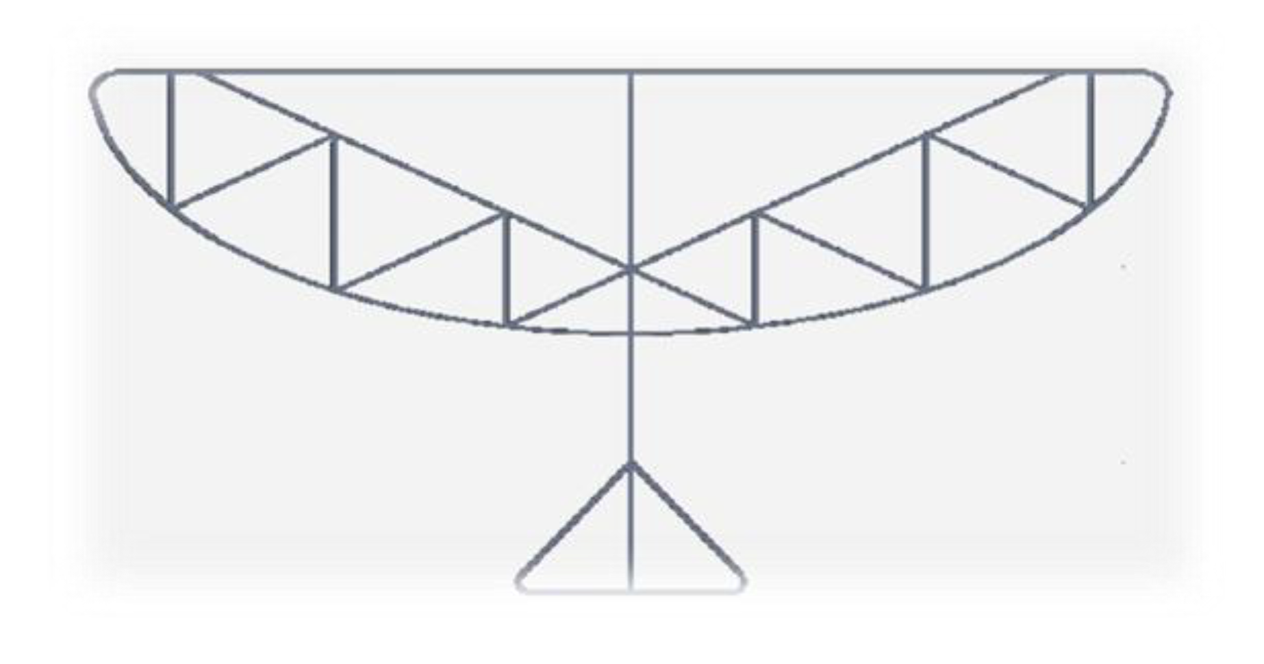
Figure 8.
CAD of fuselage.
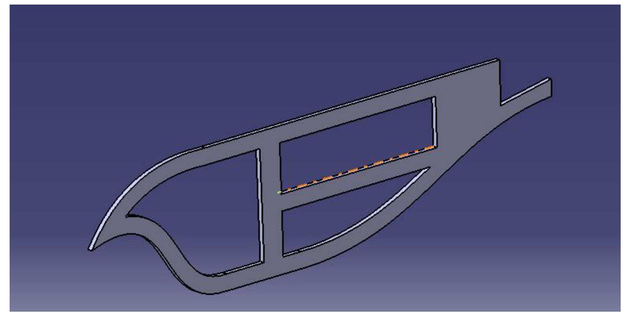
Figure 9.
CAD of Wings.
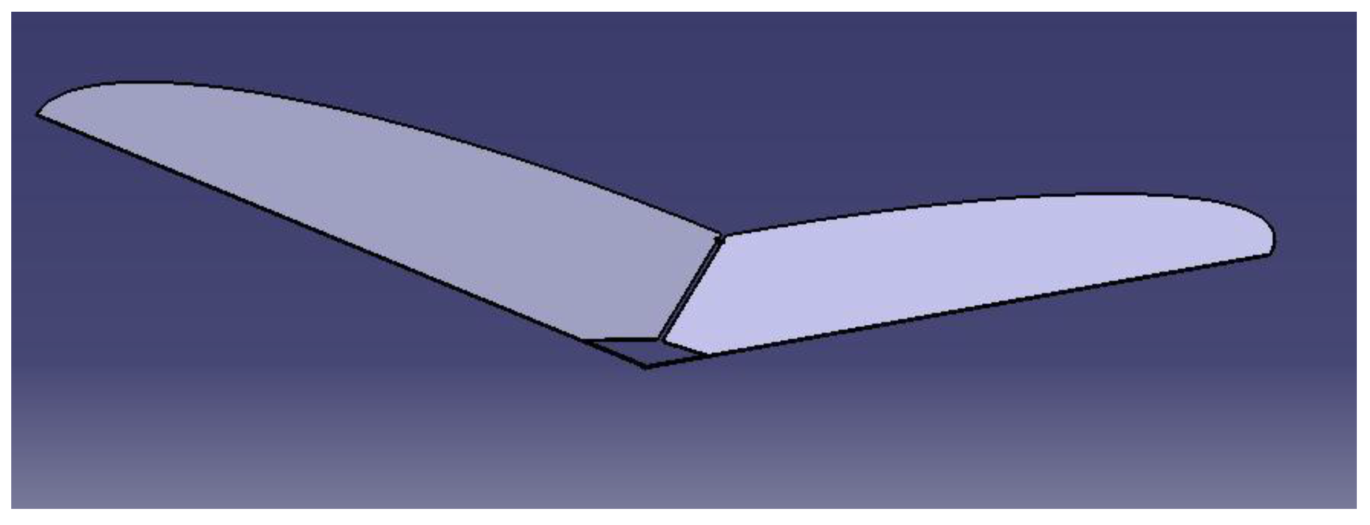
Figure 12.
Forces Generated During Upstroke and Down stroke.
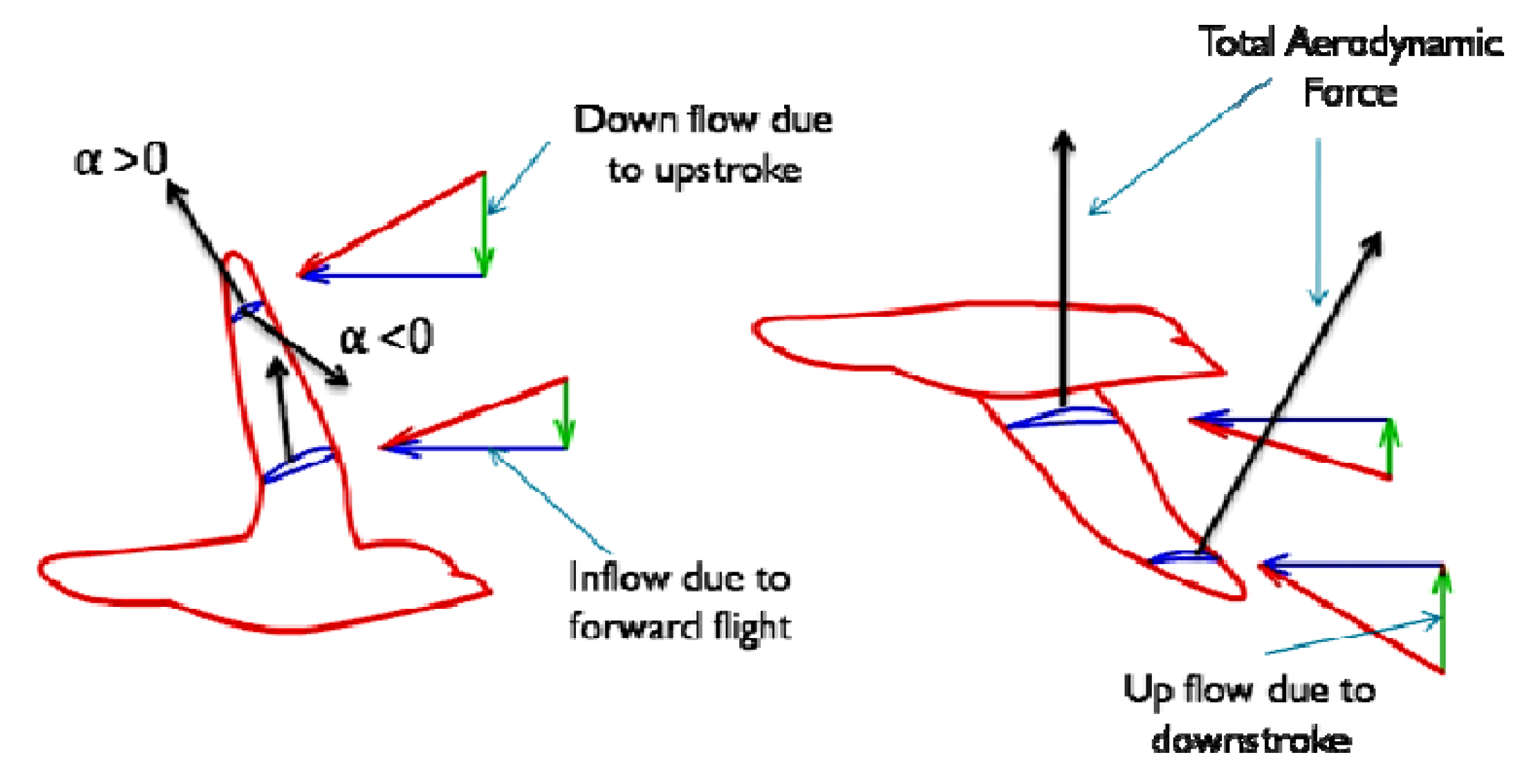
Figure 14.
Wing Form for the Analytical Study.
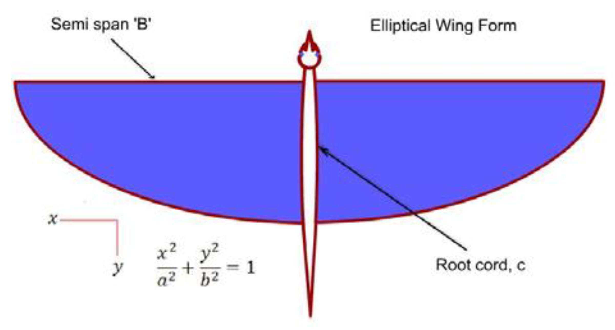
Figure 17.
Relative Air Flow.
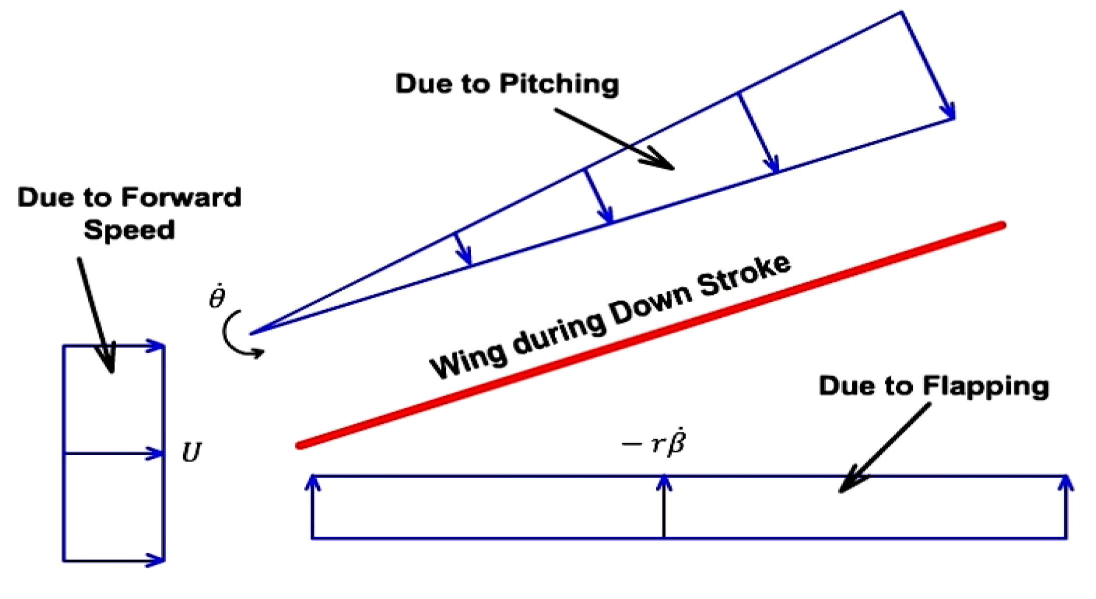
Figure 19.
Mass Limits for Ornithopter.
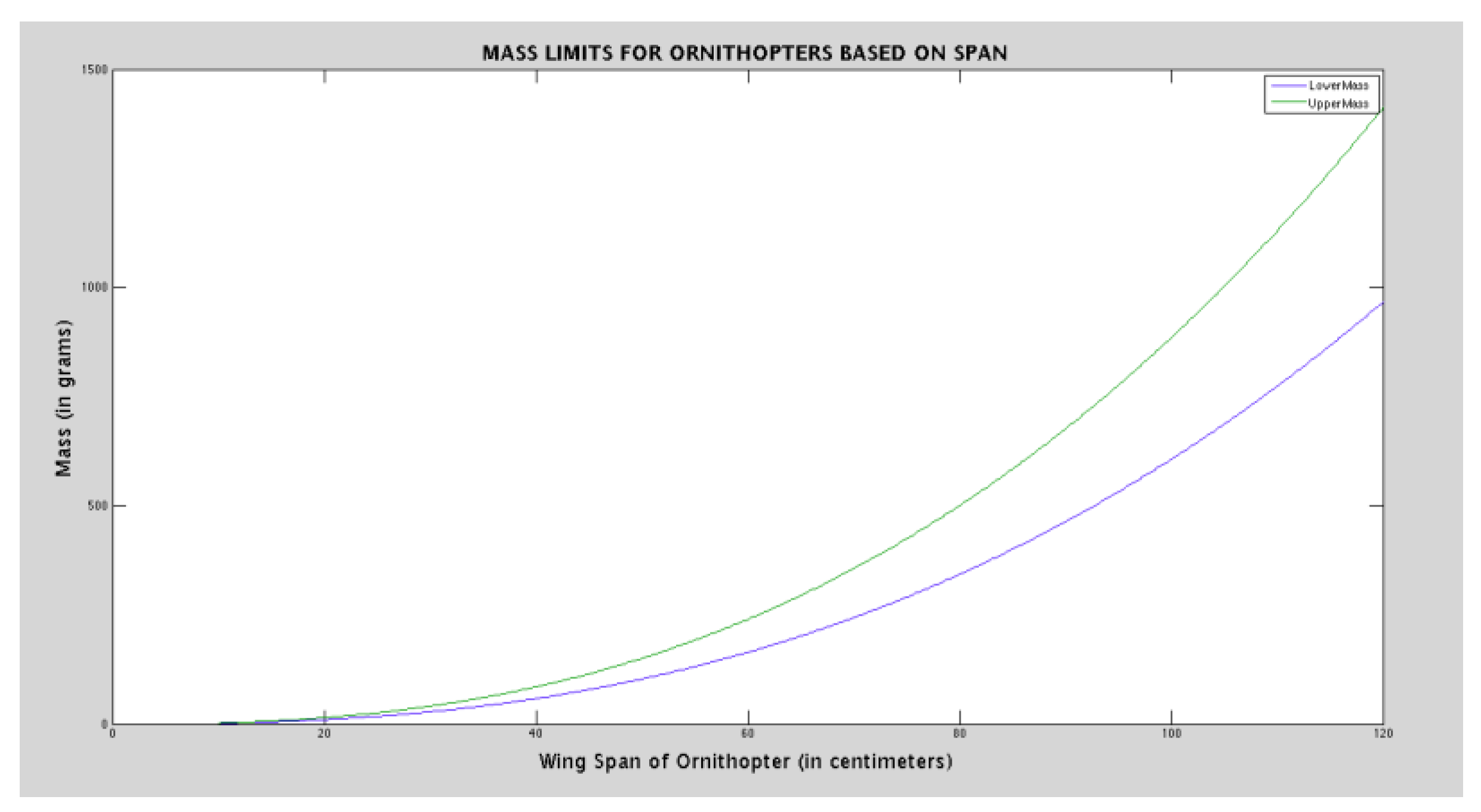
Figure 20.
Wing Area Limits for Ornithopter.
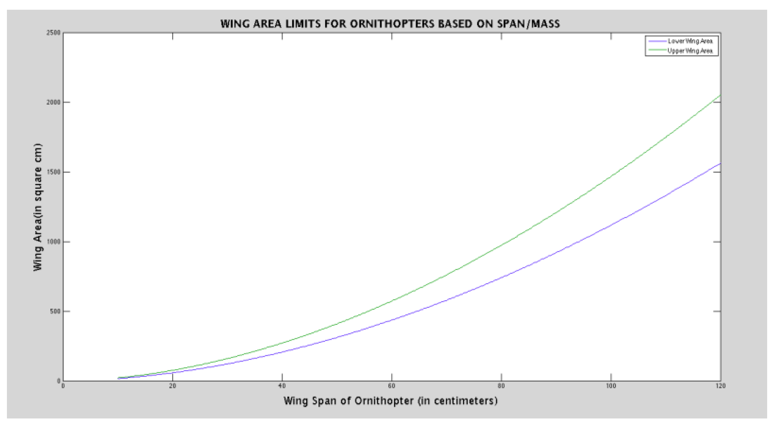
Figure 21.
Flapping Frequency Limit for Ornithopter.
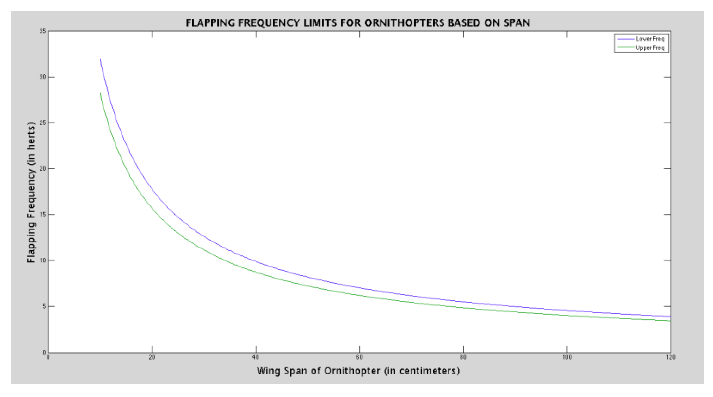
Figure 22.
Aspect Ratio Limits for Ornithopter.
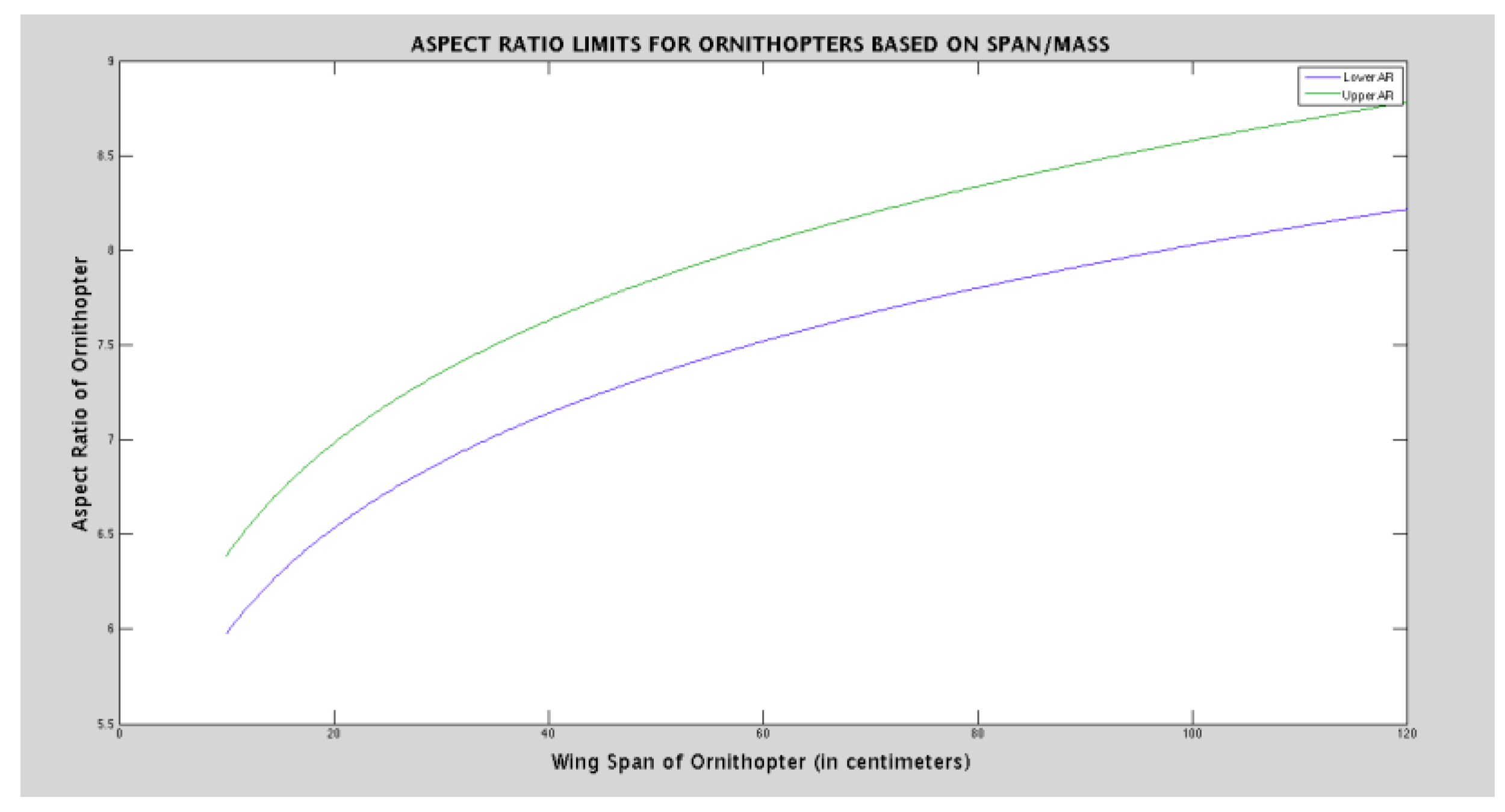
Figure 24.
Variation of leading edge in one complete cycle.
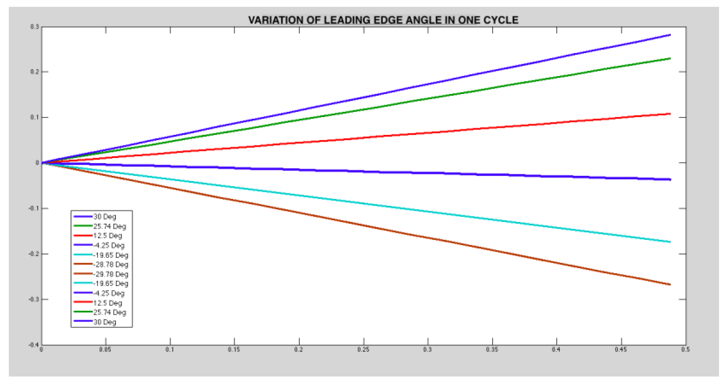
Figure 25.
Lift Force (Present Work vs Harijono [35]).
Figure 25.
Lift Force (Present Work vs Harijono [35]).
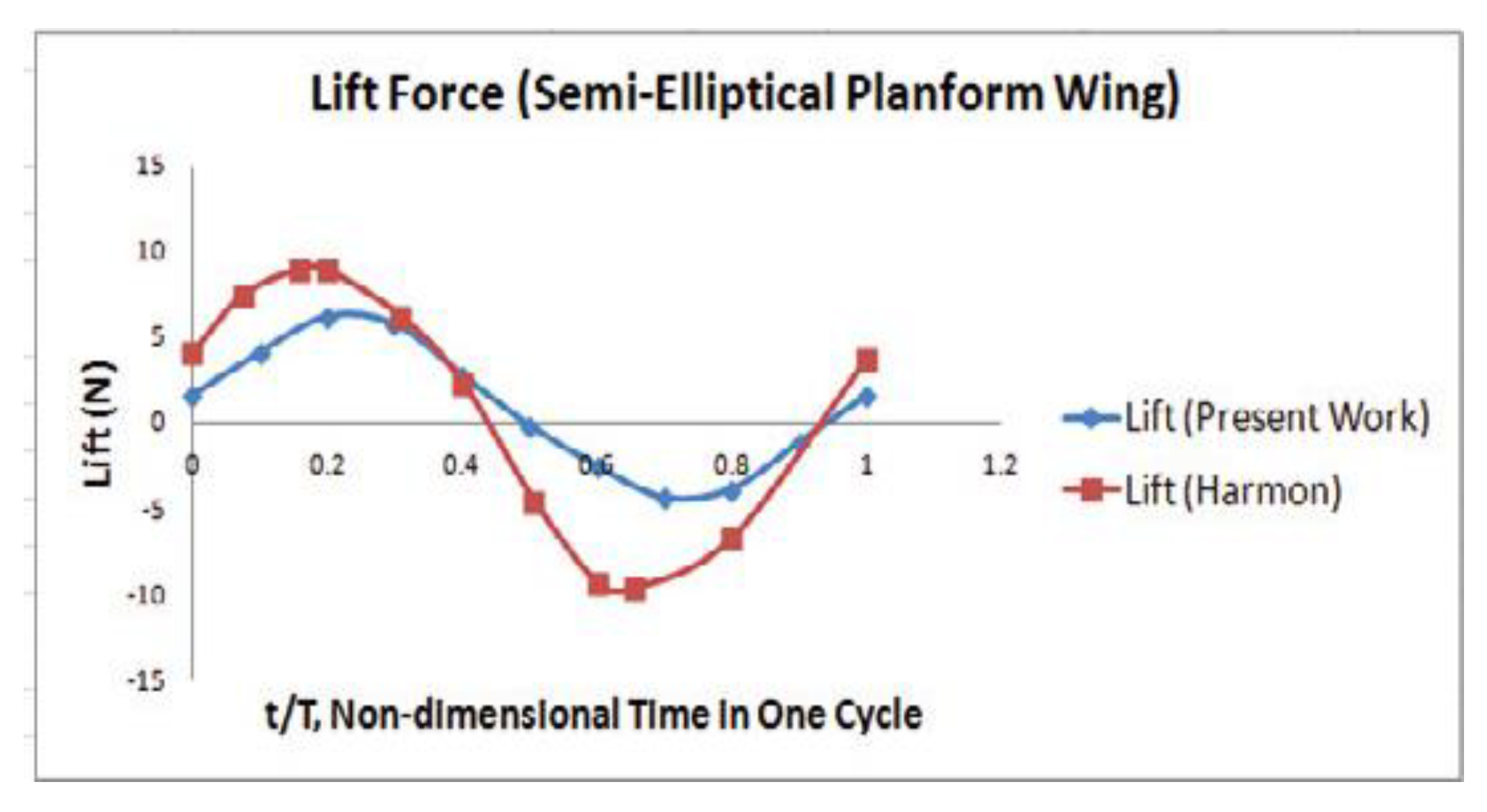
Figure 26.
Thrust Force (Present Work Vs Harjino [35]).
Figure 26.
Thrust Force (Present Work Vs Harjino [35]).

Figure 27.
Brushless Motor.
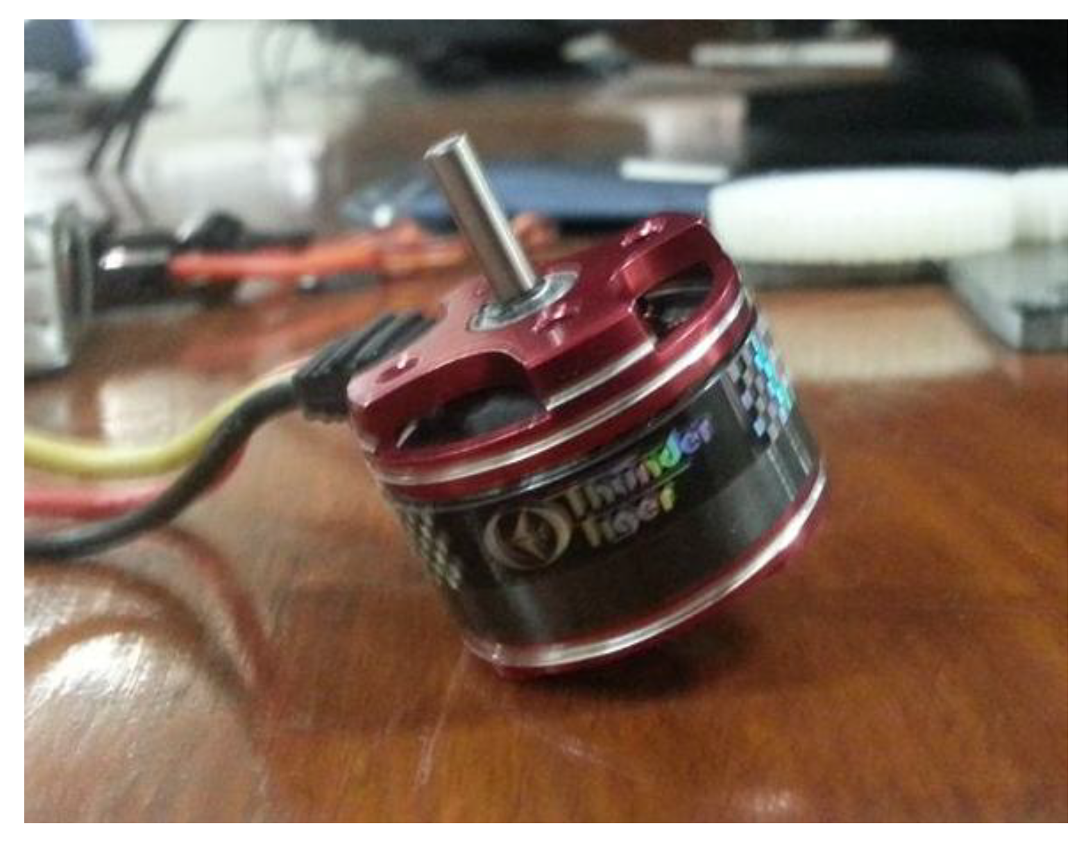
Figure 28.
Battery.

Figure 29.
Electronic Speed Controller.
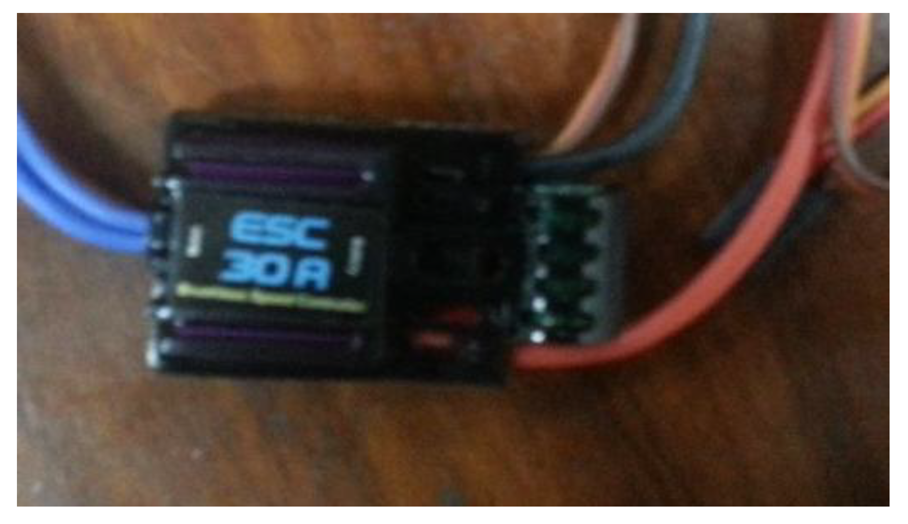
Figure 30.
Gears.
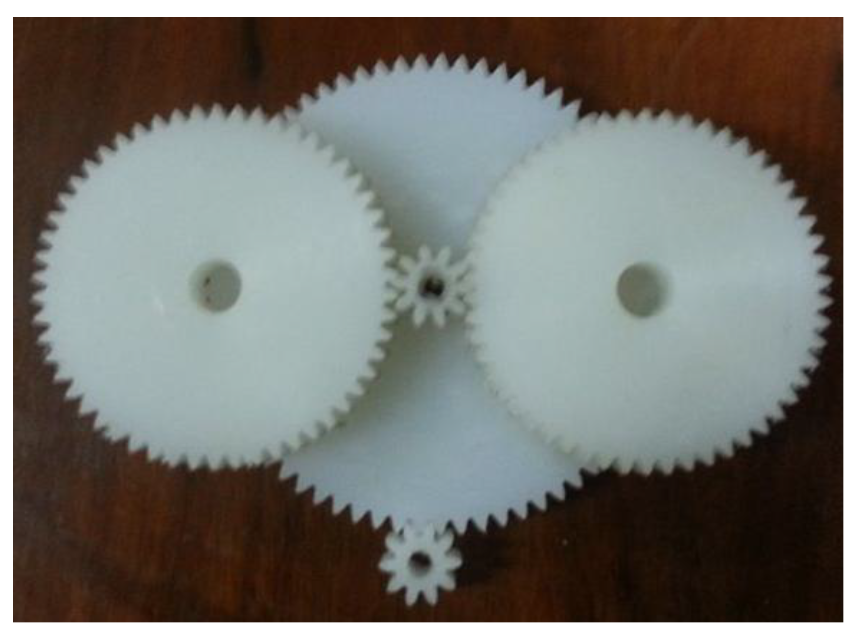
Figure 32.
Gears assembly mounted on fuselage.
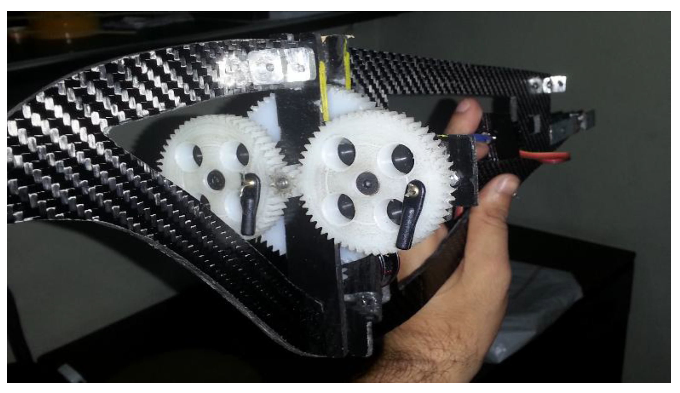
Figure 35.
Wing motion of a fly in hovering flight.
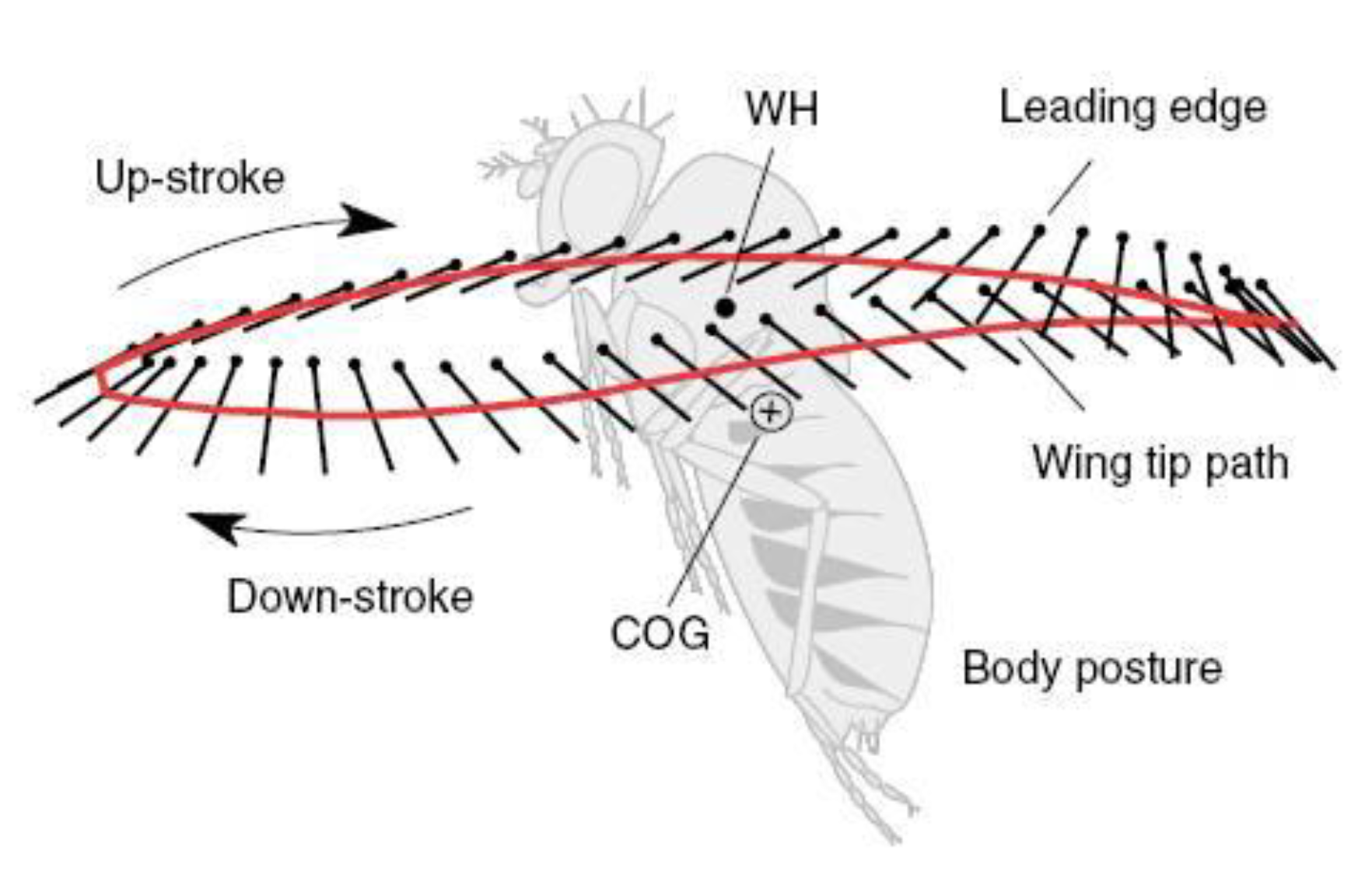
Figure 36.
One Wing.
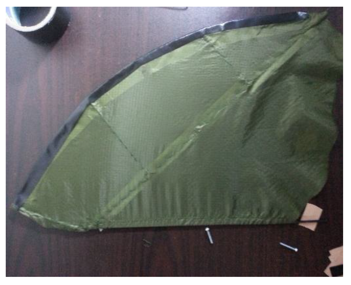
Figure 37.
Wings after complete fabrication process.
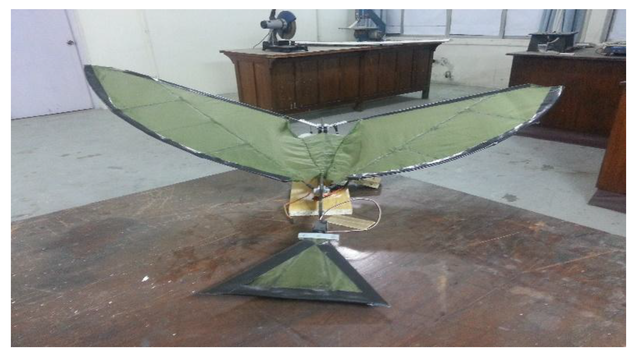
Figure 39.
Front view of assembled flapping wing micro aerial vehicle.
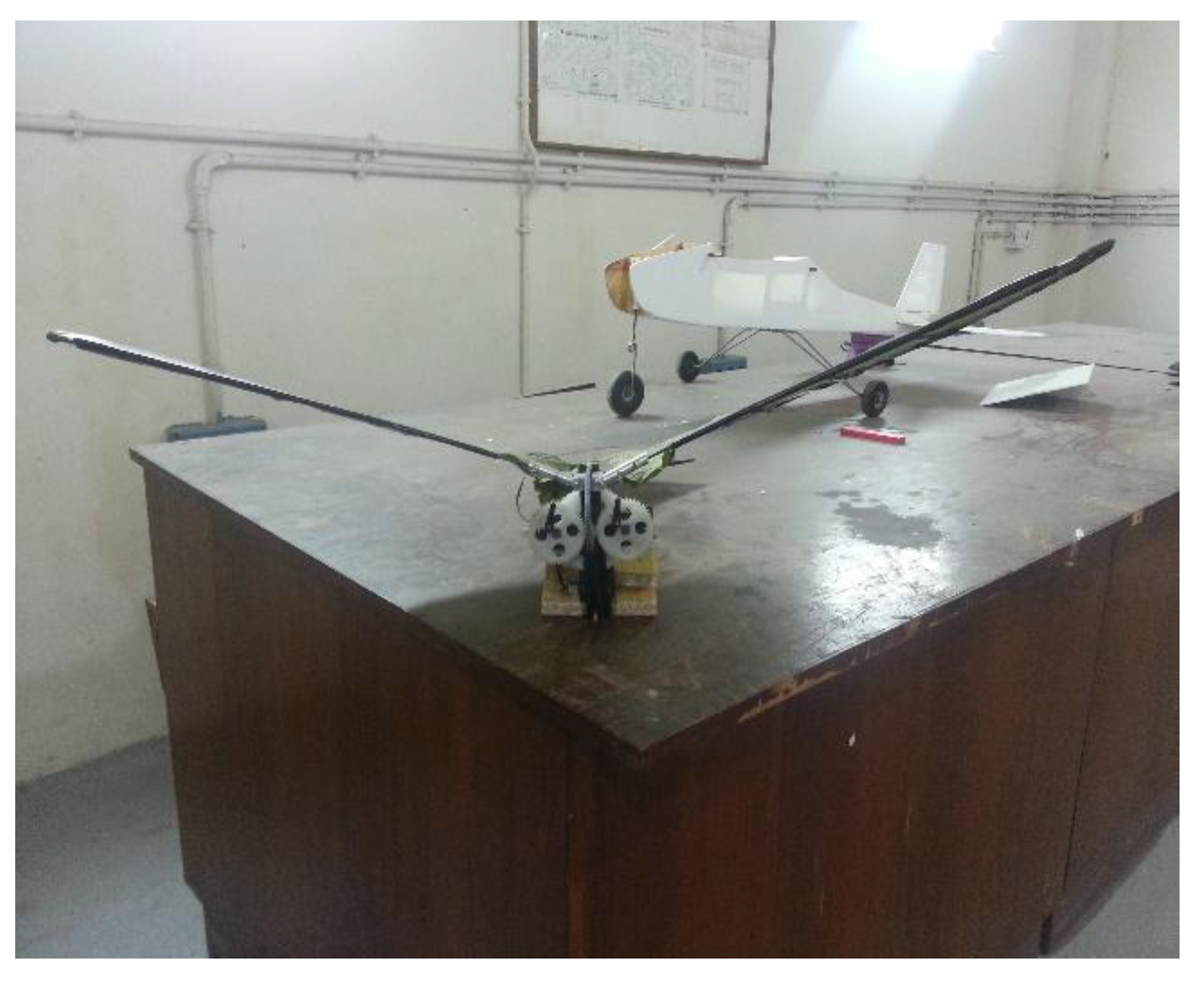
Figure 40.
Side view of assembled flapping wing micro aerial vehicle.

Table 1.
Important Parameters.
| Parameters | Formulas | Value |
|---|---|---|
| Span | Approx. | 1 m |
| Mass | (0.85×b)2.56 | .66 kg |
| Length | .70 m | |
| Wing Area | 0.16×m0.72 | .1186 m2 |
| Root Chord | (8×S)/(b×π) | .305 m |
| Flapping Frequency | 3.87×m−0.33 | 4.42 Hz |
| Upstroke angle | Approx. | 250 |
| Down stroke angle | Approx. | 300 |
Table 2.
Ornithopter Model Specification.
| Areas | Parameters | Values in cm |
|---|---|---|
| Fuselage | Length | 70 |
| Wing | Span | 100 |
| Chord | 30.5 | |
| Primary Spar | 50 | |
| Secondary Spar | 46.14 | |
| Area | 1198 | |
| Aspect Ratio | 8.348 | |
| Tail | Span | 23.59 |
| Chord | 15.25 | |
| Area | 359.8 |
Table 3.
Fuselage Specifications.
| Parameters | Values |
|---|---|
| Length | 50 cm |
| Height | 13 cm |
Table 5.
Gears Specifications.
| Gears | No. of Teeth | Pitch Diameter |
|---|---|---|
| GEAR 1 & 3 | 10 | 1.25 cm |
| GEAR 2 | 71 | 8.87 cm |
| GEAR 4 & 5 | 50 | 6.24 cm2 |
Table 6.
Tail Specifications.
| Parameters | Values |
|---|---|
| Span | 23.60 cm |
| Chord | 15.25 cm |
| Area | 360 cm2 |
Table 7.
Motor Specifications.
| Motor Specifications | |
|---|---|
| RPM/V | 1100RMP/V |
| Weight | 82 gm. |
| Dimension | 28.5mm (Dia.) x 36.5mm (Length) |
| Shaft diameter | 4mm |
| Max thrust | 1200g |
Table 8.
Battery Specifications.
| Battery Specifications | |
|---|---|
| RPM/V | 1100RMP/V |
| Weight | 82 gm. |
| Dimension | 28.5mm (Dia.) x 36.5mm (Length) |
| Shaft diameter | 4mm |
| Max thrust | 1200g |
Table 9.
Specifications of Electronic Speed Controller.
| Electronic Speed Controller Specifications | |
|---|---|
| RPM/V | 1100RMP/V |
| Weight | 82 gm. |
| Dimension | 28.5mm (Dia.) x 36.5mm (Length) |
| Shaft diameter | 4mm |
| Max thrust | 1200g |
Disclaimer/Publisher’s Note: The statements, opinions and data contained in all publications are solely those of the individual author(s) and contributor(s) and not of MDPI and/or the editor(s). MDPI and/or the editor(s) disclaim responsibility for any injury to people or property resulting from any ideas, methods, instructions or products referred to in the content. |
© 2025 by the authors. Licensee MDPI, Basel, Switzerland. This article is an open access article distributed under the terms and conditions of the Creative Commons Attribution (CC BY) license (http://creativecommons.org/licenses/by/4.0/).
Copyright: This open access article is published under a Creative Commons CC BY 4.0 license, which permit the free download, distribution, and reuse, provided that the author and preprint are cited in any reuse.


