
Submitted:
03 June 2025
Posted:
05 June 2025
You are already at the latest version
Abstract
Particle-laden flows are integral to numerous scientific and engineering disciplines, demanding a deep understanding of their rheological characteristics. Over time, various numerical methods have been developed, each offering differing levels of accuracy and analytical depth. In this study, we present a novel approach to modeling fully developed particle suspensions, aiming for simplicity and generality in solving for particle and velocity distributions. Specifically, we utilize the Carreau-Yasuda model to describe fluid viscosity as a demonstration of our proposed method. Furthermore, we investigate the impact of physical and rheological parameters on suspension flows, analyzing both particle volume fraction and velocity distributions. This research contributes to advancing the comprehension and predictive capabilities in handling complex particle-laden flows.
Keywords:
particle-laden flows
; rheology
; numerical modeling
; Carreau-Yasuda model
; suspension dynamics
1. Introduction
Fluid flows with suspended particles are found in many industrial applications such as concrete pumping [1] or extrusion and injection molding processes with filled polymers [2] [3], thus understanding the fundamentals of these flows through numerical modeling is essential. It is more important to investigate the behavior of suspension flows with generalized rheological models to have a broader range of application. We focus on steady state flows in circular tube by assuming the non-Newtonian fluids and present the simple approach of numerical modeling the particle volume fraction and velocity distributions by using the simplified form of shear-induced diffusion equation. We then present the influence of physical parameters as well as the rheological parameters of Carreau-Yasuda model on the concentration and velocity profiles. Understanding the rheology of electrode slurries is one of the applications crucial as it profoundly influences the final coating microstructure. Issues such as high slurry viscosity, which increases pressure and limits coating speed, elasticity leading to instabilities and defects, and excessive flow causing slumping and poorly structured coatings, highlight the complexities in optimizing these formulations. Due to the diverse solvent systems and components involved, pinpointing the origins of these adverse rheological properties can be challenging [4]. Additionally, precise measurement of extensional properties using miniature rheometers has revealed significant variability in slurry behavior across different formulations and binder systems [5]. The paper by Phillips et al. [6] is the fundamental reference used in this paper. They derived the shear-induced diffusion equation for the particle volume fraction () and present the corresponding no-flux boundary condition. The difference between our work and theirs is that they assume Newtonian fluid in Couette and Poiseuille flows, whereas, we consider non-Newtonian flows governed by the Carreau-Yasuda [7] model. In 2003, Chen et al. [8] studied the shear-induced particle migration in non-Newtonian flows of nickel-powder-filled polymers. They facilitated the power- law model to describe the viscosity and shear rate relation of the flow. In addition, they use the Arrhenius law to add temperature dependence to the viscosity model. It is nontrivial to solve the coupled differential equations of velocity and particle volume fraction distributions. Chen et al. [9] presented the numerical scheme to get the solutions of particle volume fraction and velocity fields for non-Newtonian flows for both steady and unsteady cases. They used the Newton-Raphson iterative method to solve the velocity fields and the finite difference method with semi-implicit scheme (known as Crank-Nicolson [10]) to solve the diffusive equation. In contrast with their paper, we use non-dimensionalization of the equations and some changes of variables techniques presented in Wang [11] to reduce the system of differential equations into a system of algebraic equations. The solution is obtained by solving numerically the nonlinear algebraic system which is computationally less intensive than the differential equations-based methods. Moreover, the Carreau-Yasuda model is more general as compared with the Power-Law used. Several other papers have been studied the different fluid flows in various processes considering the particle migration. Choi et al. [12] studies the pipe flow of pumped concrete assuming the shear-induced particle migration. They used the Bingham fluid model to describe the viscosity - shear rate relation. The commercial CFD Fluent software was used to get the numerical solutions. The paper by Siqueira and Carvalho [13] presented a numerical investigation of particle migration in a planar extrudate flow of suspensions of some hard spheres. In particular, they studied the Newtonian flow in parallel-plates and then the extruded flow in the ambient atmosphere. The numerical solutions have been obtained by the stabilized finite element method together with the elliptic mesh generation method to compute the position of the free surface. Rebouças et al. [14] studied the fully-developed suspension flow in a circular tube and the effects of particle and shear-induced viscosity. Their work is similar to ours in the sense that they also presented the numerical solution of shear-induced diffusion equation with the assumption of non-Newtonian flow and investigated the effects of average particle volume fraction on the concentration and velocity profiles. Moreover, the results of both concentration and velocity profiles for different bulk concentration () of the suspensions and the parameter agree with our numerical solutions. The difference between their approach and ours is that they used the procedure to overcome the singularity of the model near the centerline of the tube. Also they used Cross model to describe the fluid viscosity whereas we use the Carreau-Yasuda model that has more parameters (with extra variable a). Another difference is that we present the effects of the whole range of parameters including the pressure gradient, average particle volume fraction, all 5 parameters of Carreau-Yasuda and the model parameter (thereafter ). In addition to numerical studies, Rueda [15] presented a complete experimental study of the rheological characteristics of suspension flows. In particular, the author evaluates the influence of various parameters on the viscosity.
2. Model and Methods
2.1. Governing Equations of Fluid
The flow is governed by equation of continuity for an incompressible mass
the conservation equation of linear momentum
and the Newton’s Law of viscosity
2.2. Particle Poiseuille Flow Through a Cylindrical Tube
Let denote the particle fraction. Consider the Krieger & Dougherty [16] model with the following terms on particle volume induced relative viscosity
and convective diffusion of particles satisfying the conservation equation for the particle volume fraction
According to Phillips et al. [6], can be neglected for very large Peclet number . Then replacing the flux terms in (5) with the equations from (4) gives us
Since we are considering the flow in cylindrical tube, the divergence is in general form. No-flux boundary condition at the wall which is represented as
So, combining (6) and (7), we get the generalized system of differential equations of velocity profile and particle volume fraction distribution, which is
with the no-flux boundary condition at the wall
2.3. Steady State Velocity and Particle Distributions
In steady state flow, and we assume the r-direction, so the second equation in the coupled system (8) becomes
which can be integrated over r and applying the no-flux boundary condition to compute the constant of integration, we get
which means no-flux everywhere in suspension in steady-state scenario. This equation can be integrated with the boundary condition at the wall, so we get the following simplification
Now we want to simplify the system. By rearrangement of the first part of the coupled system (8) we get
and integration of (13) gives us
applying the boundary case (at ), we get the constant of integration . So, we have the simplified equation
Summarizing the coupled ODE for steady-state case, we have the following system of differential equations
2.4. Nondimensionalization and Numerical Details
In order to further simplify the coupled system (16), we introduce the nondimensional variables as following
Substituting the new variables (17) into (16) gives us the system in nondimensional form as
At the wall we have , , and , and the first equation in (18) becomes,
where is the magnitude of the pressure gradient. Suppose we use the Krieger-Dougherty equation for and the Carreau-Yasuda model for as in (4), we have
Combining Eqs. 19 and 20 gives
Here, is taken to be . Given , , and R, we can obtain by solving the above nonlinear equation (Eq. 21) for . Once is obtained, then it is straightforward to obtain , which is used as the unit for viscosity. Using the identity shown in Eq. 19, we can rewrite Eq. 18 as
where and is taken to be in this work, following Phillips et al. [6]. Again, using the Krieger-Dougherty equation for and the Carreau-Yasuda model for , we have
where
Here, , , and . The term is the time constant in dimensionless form, using as the characteristic time scale. Combining Eqs. (22) and (23), we have
and combining Eqs. (22)-(24), we have
From the above two equations, Eqs.(26) and (27), one can easily obtain the volume fraction , the shear rate distribution , and the volume fraction as a function of the shear rate, . The velocity distribution can be obtained using the method of Wang (2021, under review). Using as the unit for velocity, i.e., , we have
Once the shear rate distribution is obtained, it is straightforward to obtain by solving the above ODE numerically.
If we try to solve the system for s, complications in the numerical computations arise, for instance, is highly nonlinear. Thus, following the idea from the paper of Wang (2021), it is wise to solve for instead of s. This means, given , we want to solve for and which can be easily obtained by root finding () the following equation
and substituting the solution back to one of the equations (26) or (27) to find . Because is required to solve the system, with given , it can be estimated by using the concept of binary search or so-called "interval halving method". Since is always less than the , we know that the true is greater than 0 and less than . By using this information, we can find the the corresponding that is shown as an intermediate step in Figure 1.
3. Results and Discussion
3.1. Verification and Validation of Numerical Results
Now we want to generate some output by using the algorithm shown in Figure 1. The Python programming language was used to implement the numerical algorithm. We assume that the fluid viscosity is described by the Carreau-Yasuda model. The following table represents the constant values we chose to use as a base in the computations. Figure 2 and Figure 3 show the numerical solutions of the system.
The solutions of particle volume fraction () and the dimensionless shear rate (s) distributions are shown in Figure 2a,b. The dimensionless velocity () profile in Figure 3a is computed from the integration of the simple ODE (28). The iterative behavior of the inner algorithm that finds the best approximation of is shown in Figure 3b.
To verify the numerical model and the corresponding Python code used to solve for and s, we back-substitute these solutions into the system (Eqs. 26, 27 labeled as and , respectively) and check the errors. As we can notice, the errors are considerably small with the order of (Figure 3).
3.1.1. Newtonian Fluid
In this section, the validation of our numerical algorithm in comparison with Phillips et al.’s [6] analytical solution is presented. Authors of the analytical solution of the equation governing at steady state presented the explicit formula for as
where . This explicit formula describes the particle volume fraction distribution at steady state Newtonian case. We compare our numerical algorithm with the analytical solution for different and the result is shown in Figure 4.
We can see that our numerical solution perfectly agrees with their results.
3.1.2. Power-Law Fluid
Next, let us consider the viscosity defined by power-law model as following
where K is the fitted parameter and n is the power-law index. We incorporate this equation into our numerical algorithm to solve for concentration profiles for different values of power-law index n. To validate our numerical approach, let us derive the analytical solution in a similar way presented by Phillips et al. [6]. From Eq. 15 we have
and substituting this formula into Eq. 12 gives us
Letting with yields the analytical solution for the fully-developed steady-state power-law fluid as
Figure 5 shows both analytical solution from the above derivation and our numerical solution for different power-law index n. Interestingly, when , that is , vanishes and the solution of Eq. 38 is constant for any value of . For values the concentration profiles are higher near the centerline and lower near the wall of the circular tube, however if we observe very small particle volume fraction near the centerline and it increases towards the wall. From this special case, we can conclude that for and the particle volume fraction distribution is exactly flat at . Generally speaking, when in Eq. 38 the concentration profile is along the radial position.
3.1.3. Other Relative Viscosity Models
3.2. Influence of Average Particle Volume Fraction
Now we analyze the influence of the parameter change on the output. In particular, we will alter one parameter at a time while keeping everything else fixed (as in Table 1) and observe the change in the output. The parameters that will be altered are the average particle volume fraction (), pressure drop (), the Carreau-Yasuda model parameters, and the . First, let us consider the effect of average volume fraction on the output results.
We change the values of the average particle volume fraction from 0.1 to 0.4 while keeping other parameters fixed (as in Table 1). In Figure 7a, the concentration profile moves upward as increases. This observation is as expected as the result in Figure 7b where the relation between and lies below the diagonal line which agrees with the theory that . We can also see that the velocity profile decreases with the increasing average particle volume fraction (Figure 7c). Correspondingly, the average velocity decreases as well (Figure 7d). In general, the plots in Figure 7 suggest that the particle volume fraction and velocity distribution is highly dependant on the average particle volume fraction.
3.3. Influence of Pressure Gradient
Next, we want to see the influence of pressure drop on the output, so we vary it from Pa to Pa, and keep everything else constant (as in Table 1).
The behavior of the concentration profile is not uniform, since, in Figure 8a, it decreases near the centerline () but increases near the wall () as the pressure drop increases. Clearly, the vs. curve moves upwards as shown in Figure 8b, and the velocity profile increases as well as the average velocity (Figure 9a,b) with the increasing pressure drop. Overall, we can see that seemingly the pressure drop affects the velocity profile, but has weak relation with the particle volume fraction.
3.4. Influence of Carreau-Yasuda Parameters
Our next analysis examines the effect of the viscosity at infinite shear rate, , which was varied from 100 to 700 Pa·s.
We can notice the higher value of leads to a slight increase near the center and slight decrease of particle volume fraction distribution () near the wall in Figure 10a. The and relation curve moves downwards as shown in Figure 10b. The velocity decreases gradually as well as the average velocity with the increase of (Figure 10c,d).
Somehow strong impact is observed on the velocity profile, but the concentration profile stays almost unaffected. Same behavior is shown in Figure 11 when we increase the from 1000 Pa·s to 7000 Pa·s. No considerable influence is made by the change of dimensionless parameter a as can be seen from Figure 12. In particular, the velocity profile decreases by increasing a, but stops changing regardless the change in the parameter (Figure 12c) which is same for the average velocity.
Interestingly, the time constant of Carreau-Yasuda model affects the output of and v curves to a high extent. When we vary the parameter from 1.2 s to 5 s, in Figure 13a, the distribution decreases near the centerline () and increases near the wall (). However almost no change is observed about .
The relation curve between and moves upward as shown in Figure 13b, and the velocity profile as well as the average velocity linearly increase with the increasing as demonstrated in Figure 13c,d).
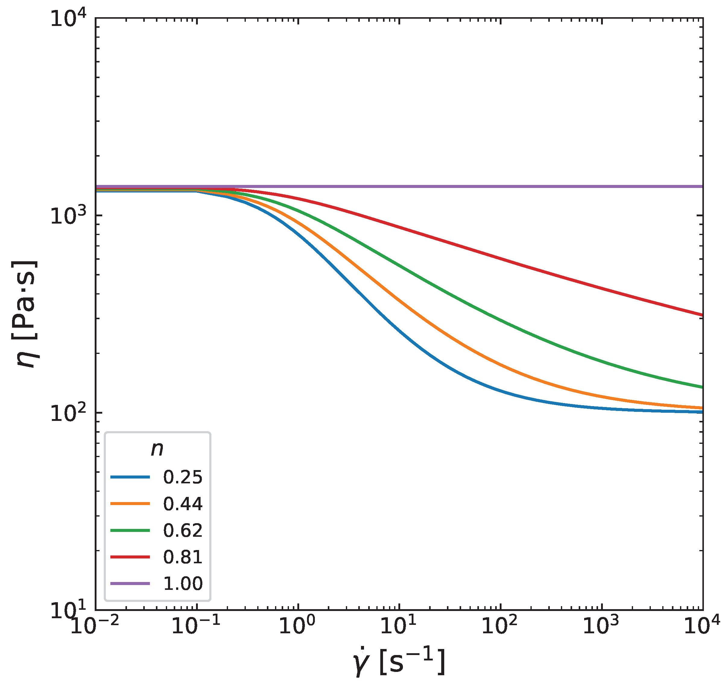
The parameter n was varied from 0.1 to 1 and the concentration profile is less near the wall and is more near the center as shown in Figure 14a. This means that if we assume the Newtonian fluid rheology, this would model the concentration distribution with higher values closer to the center and lower values closer the wall. The velocity profile and average velocity decrease as n goes towards 1 (Figure 14c,d).
3.5. Influence of Other Model Parameters
The fitting parameter, , took the values from 0.4 to 0.95. This change affected the output considerably (Figure 15 and Figure 16). In particular, the particle volume fraction distribution is higher near the center and is lower near the wall. There is a point about where does not change. The velocity profile and average velocity increase gradually as increases.
4. Conclusions
In this study, fully-developed fluid flows with filled particles in circular tube were analyzed. The Carreau-Yasuda and Krieger & Dougherty models were used to describe the particle-filled fluid and effective viscosities. respectively. The well-known diffusive flux model, proposed by Phillips et al. [6], was taken as a base of our analysis. The model was simplified by means of the non-dimensionalization technique and corresponding numerical method was applied for the solution. The verification was achieved by back-substituting the solution to the model that showed very small error. With simplicity of our approach, the influence of particle and flow distributions by the model and the rheological parameters were observed. In particular, both particle concentration and velocity profiles showed strong dependancy on the relation with the rheology parameters , n and model parameter and . The particle volume fraction distribution was weakly varied by the change in pressure gradient and rheology parameters , and a, but they strongly affected the velocity profile.
For future research, the circuit network method [19] offers a promising avenue for further investigation. This method could be particularly useful for studying similar fluid dynamics in more complex scenarios, such as coating and extrusion die manifolds, where the behavior of particle-filled fluids in confined geometries presents additional challenges and opportunities for analysis.
Author Contributions
Conceptualization, M.A. and D.W.; methodology, M.A.; software, M.A.; validation, M.A., Y.W. and D.Z.; formal analysis, M.A.; investigation, M.A.; resources, D.W. and A.P.; data curation, M.A.; writing—original draft preparation, M.A.; writing—review and editing, M.A., Y.W. and D.Z.; visualization, M.A.; supervision, D.W.; project administration, D.W.; funding acquisition, D.W. All authors have read and agreed to the published version of the manuscript.
Funding
This research was funded by Nazarbayev University under the Research Grant Program No. SEDS2023010
Institutional Review Board Statement
Not applicable
Informed Consent Statement
Not applicable
Data Availability Statement
The authors confirm that the Python source code of the results is publicly available at GitHub
Acknowledgments
During the preparation of this manuscript, the authors used ChatGPT (OpenAI, GPT-4, May 2025 version) to assist with LaTeX formatting of figures, including restructuring subfigure layouts and standardizing image paths. The authors have reviewed and edited the output and take full responsibility for the content of this publication.
Conflicts of Interest
The authors declare no conflicts of interest.
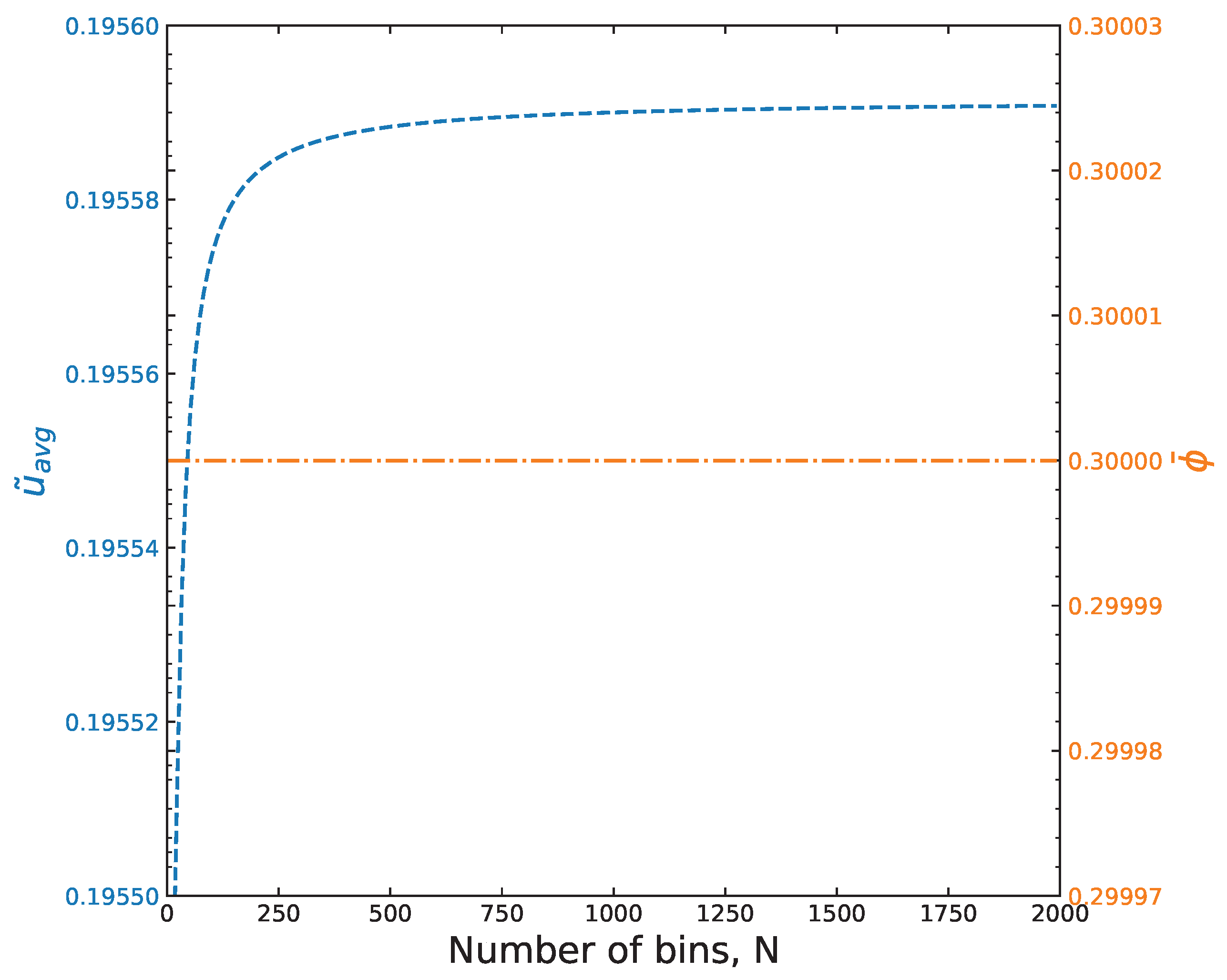
Appendix A. Function Error and Optimal Mesh Size in Numerical Computations
Figure A1.
Absolute errors of the system with Carreau-Yasuda viscosity model.
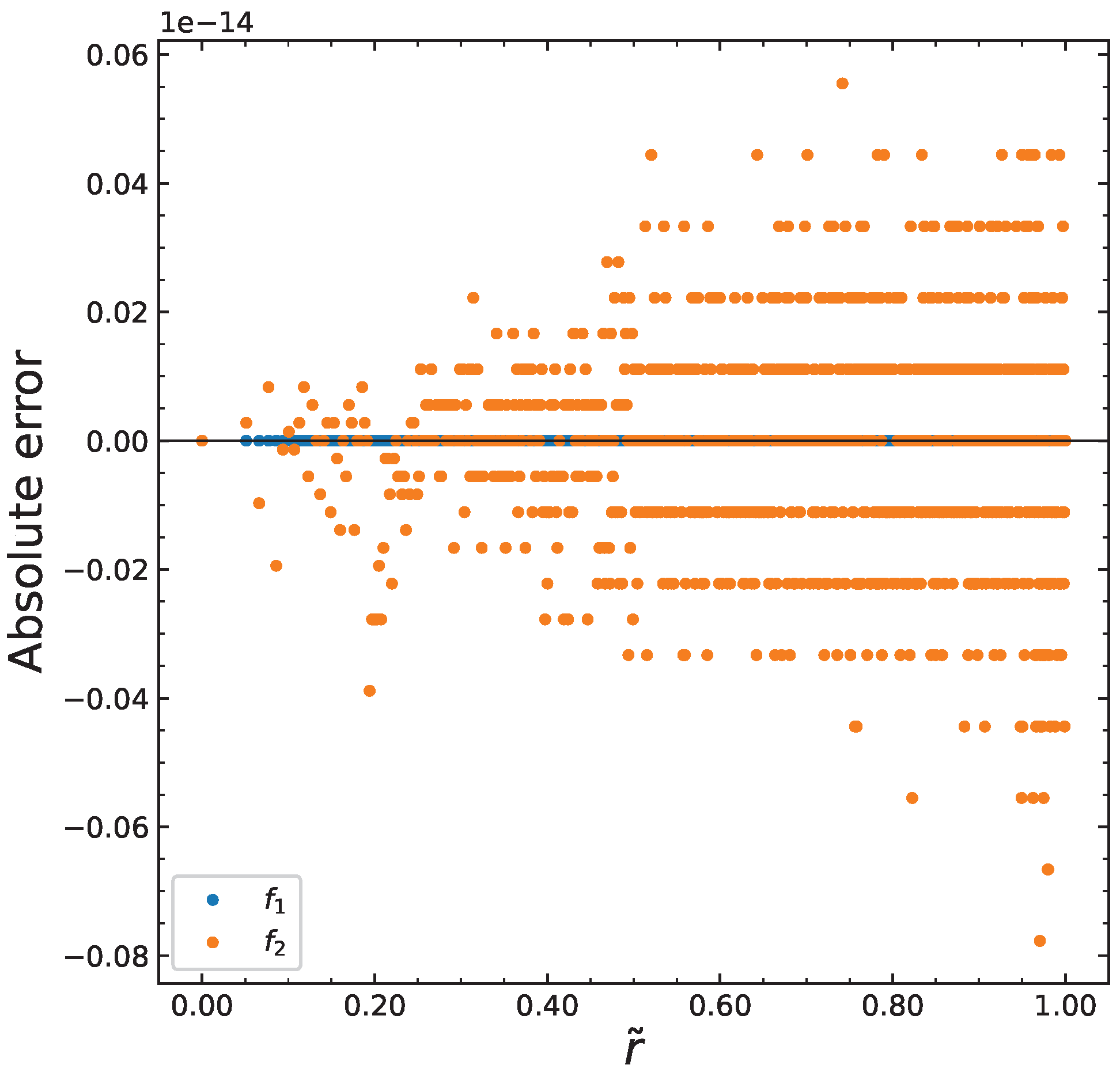
Figure A2.
Average velocity and average particle volume fraction at various number of bins.
Appendix B. Influence of Carreau-Yasuda model parameters on viscosity
Figure A3.
Influence of change in on the viscosity
Figure A4.
Influence of change in on the viscosity
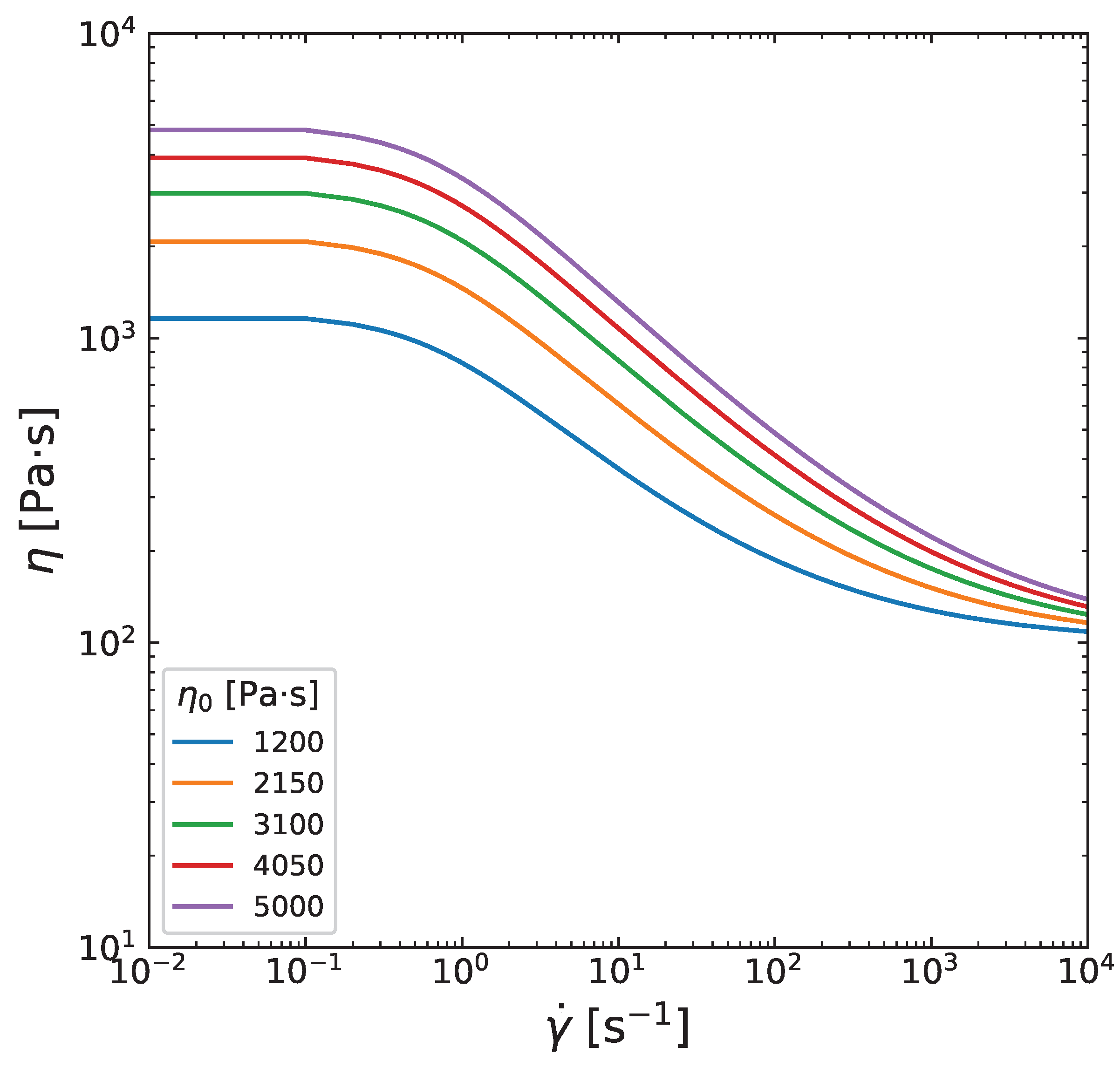
Figure A5.
Influence of change in a on the viscosity
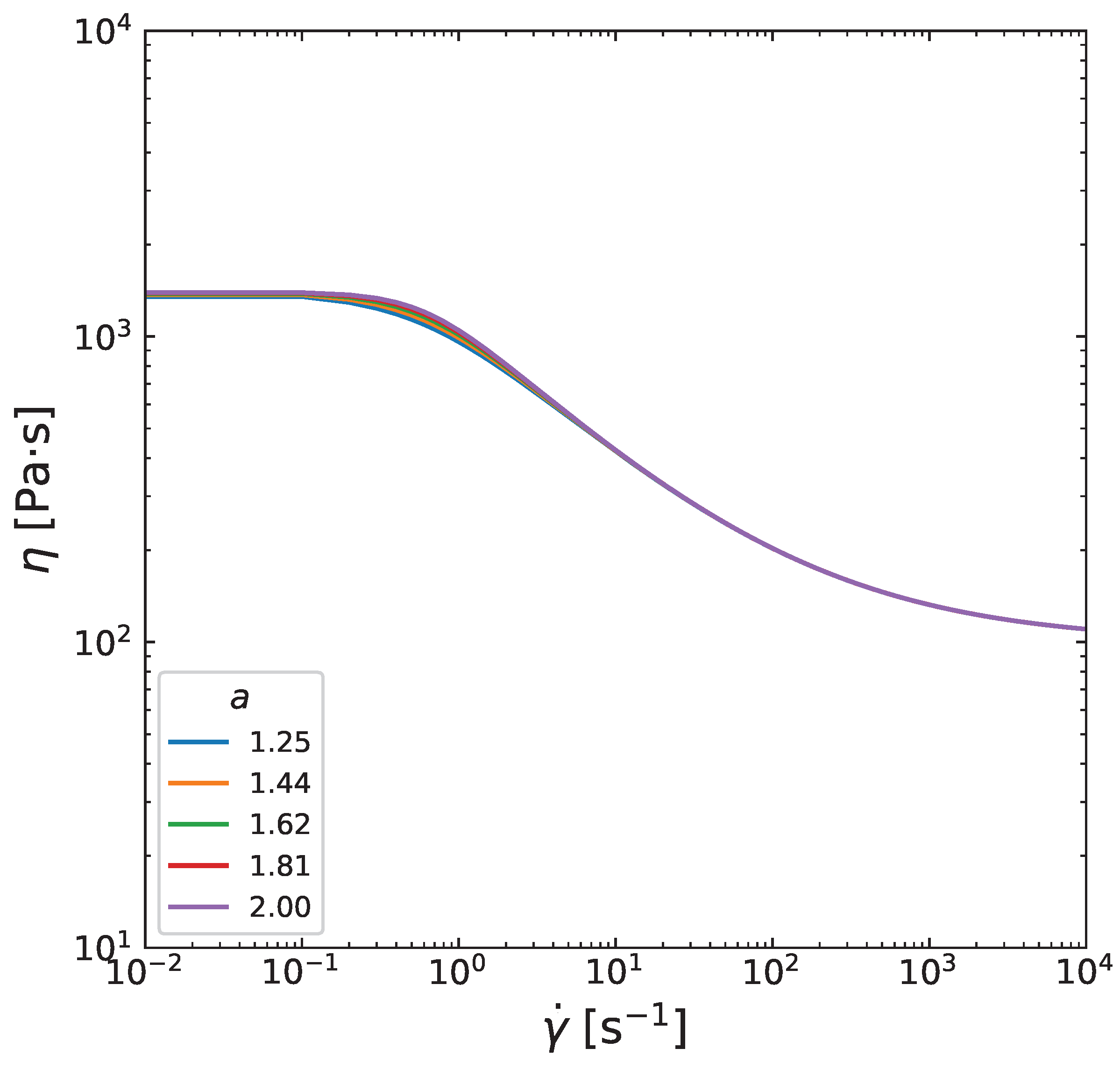
Figure A6.
Influence of change in on the viscosity
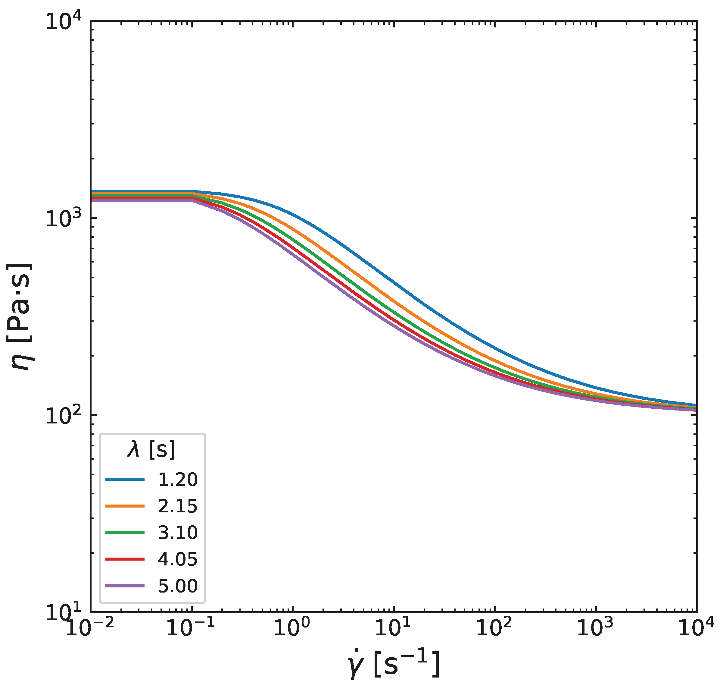
Figure A7.
Influence of change in n on the viscosity
References
- Xie, X.; Zhang, L.; Shi, C.; Liu, X. Prediction of lubrication layer properties of pumped concrete based on flow induced particle migration. Construction and Building Materials 2022, 322. [Google Scholar] [CrossRef]
- Rueda, M.; Auscher, M.; Fulchiron, R.; Périé, T.; Martin, G.; Sonntag, P.; Cassagnau, P. Rheology and applications of highly filled polymers: A review of current understanding. Progress in Polymer Science 2017, 66, 22–53. [Google Scholar] [CrossRef]
- Quintana, J.; Heckner, T.; Chrupala, A.; Pollock, J.; Goris, S.; Osswald, T. Experimental study of particle migration in polymer processing. Polymer Composites 2019, 40(6), 2165–2177. [Google Scholar] [CrossRef]
- Reynolds, C.D.; Hare, S.D.; Slater, P.R.; Simmons, M.J.H.; Kendrick, E. Rheology and Structure of Lithium-Ion Battery Electrode Slurries. Energy Technology 2022, 10, 2200545. [https://onlinelibrary.wiley.com/doi/pdf/10.1002/ente.202200545]. [CrossRef]
- Reynolds, C.; Lam, J.; Yang, L.; Kendrick, E. Extensional rheology of battery electrode slurries with water-based binders. Materials & Design 2022, 222, 111104. [Google Scholar] [CrossRef]
- Phillips, R.; Armstrong, R.; Brown, R.; Graham, A.; Abbott, J. A Constitutive Equation for Concentrated Suspensions that Accounts for Shear- Induced Particle Migration. Physics of Fluids A: Fluid Dynamics 1992, 4(30), 30–40. [Google Scholar] [CrossRef]
- Bird, R.; Armstrong, R.; Hassager, O. Dynamics of polymeric liquids. Volume 1., 2nd ed.; John Wiley & Sons: New York, 1987. [Google Scholar]
- Chen, X.; Tan, K.; Lam, Y.; Chai, J. The Transverse Particle Migration of Highly Filled Polymer Fluid Flow in a Pipe. Innovation in Manufacturing Systems and Technology (IMST) 2003. Available at http://hdl.handle.net/1721.1/3757.
- Chen, X.; Lam, Y.; Tan, K.; Chai, J.; Yu, S. Shear-Induced Particle Migration modelling in a concentrated suspension flow. Modelling Simul. Mater. Sci. Eng. 2003, 11(4), 503–522. Available at https://iopscience.iop.org/article/10.1088/0965-0393/11/4/307. [CrossRef]
- Cebeci, T. Convective heat transfer., 2nd ed.; Springer-Verlag Berlin and Heidelberg GmbH & Co. KG: Berlin, Germany, 2002. [Google Scholar]
- Wang, Y. Steady isothermal flow of a Carreau–Yasuda model fluid in a straight circular tube. Journal of Non-Newtonian Fluid Mechanics 2022, 310, 104937. [Google Scholar] [CrossRef]
- Choi, M.; Kim, Y.; Kwon, S. Prediction on pipe flow of pumped concrete based on shear-induced particle migration. Cement and Concrete Research 2013, 52, 216–224. [Google Scholar] [CrossRef]
- Siqueira, I.; Carvalho, M. Particle migration in planar die-swell flows. J. Fluid Mech. 2017, 825, 49–68. [Google Scholar] [CrossRef]
- R.B.Rebouças.; Siqueira, I.; de Souza Mendes, P.; Carvalho, M. On the pressure-driven flow of suspensions: Particle migration in shear sensitive liquids. Journal of Non-Newtonian Fluid Mechanics 2016, 234, 178–187. [Google Scholar] [CrossRef]
- Rueda, M. Rheology and processing of highly filled materials. Materials. Universite de Lyon 2017. [Google Scholar]
- Krieger, I.; Dougherty, T. A Mechanism for Non-Newtonian Flow in Suspensions of Rigid Spheres. Transactions of the Society of Rheology 1959, 3(137). [Google Scholar] [CrossRef]
- J.S. Chong, E.C.; Baer, A. Rheology of concentrated Suspensions. Journal of Applied Polymer Science 1971, 15, 2007–2021. [Google Scholar] [CrossRef]
- Quemada, D. Rheology of concentrated disperse systems and minimum energy dissipation principle. Rheologica Acta 1977, 16, 82–94. [Google Scholar] [CrossRef]
- Razeghiyadaki, A.; Wei, D.; Perveen, A.; Zhang, D.; Wang, Y. Effects of Melt Temperature and Non-Isothermal Flow in Design of Coat Hanger Dies Based on Flow Network of Non-Newtonian Fluids. Polymers 2022, 14. [Google Scholar] [CrossRef] [PubMed]
Figure 1.
Proposed algorithm flowchart
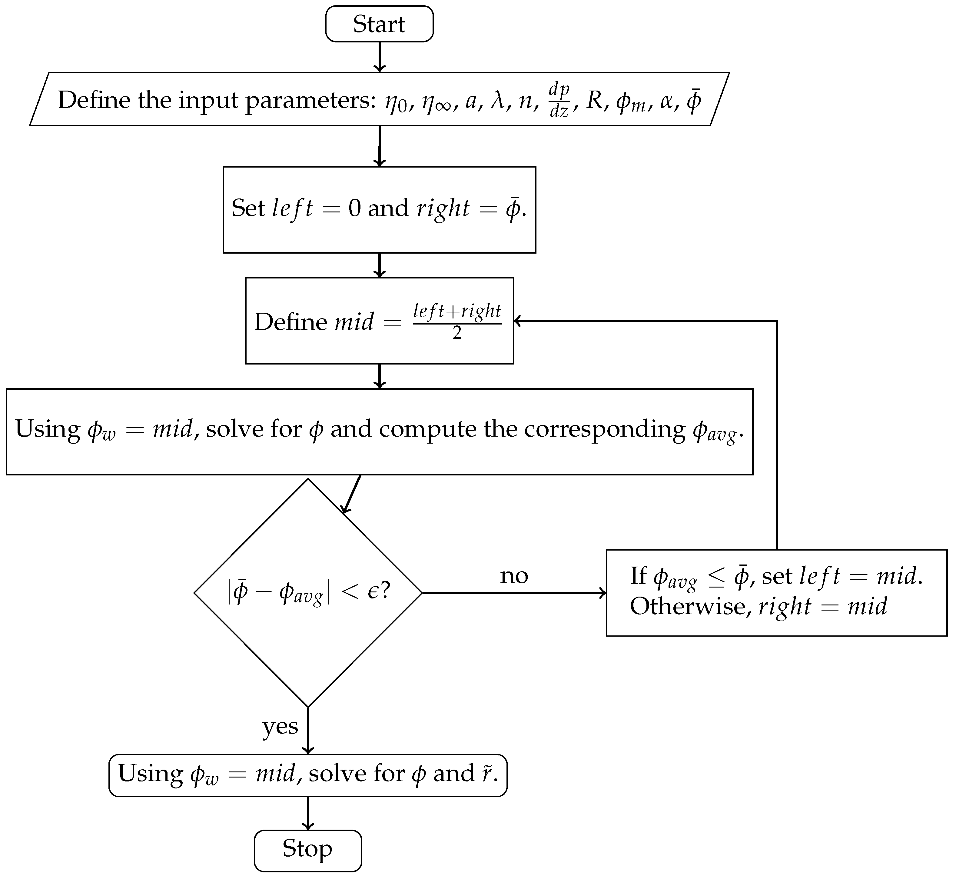
Figure 2.
The results of the numerical algorithm.
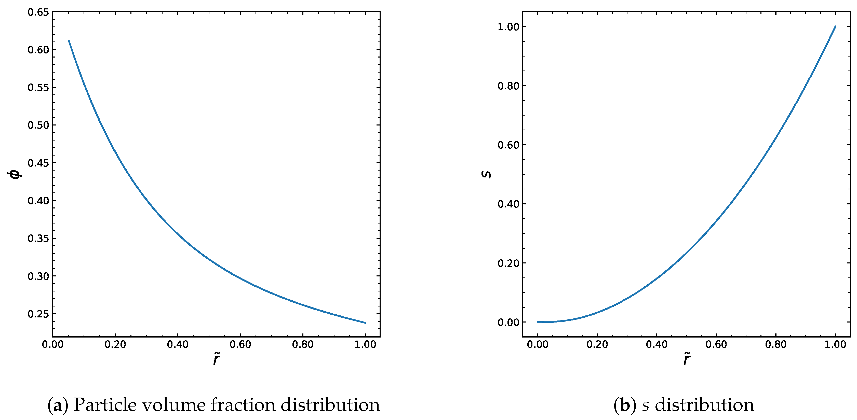
Figure 3.
The results of the numerical algorithm.
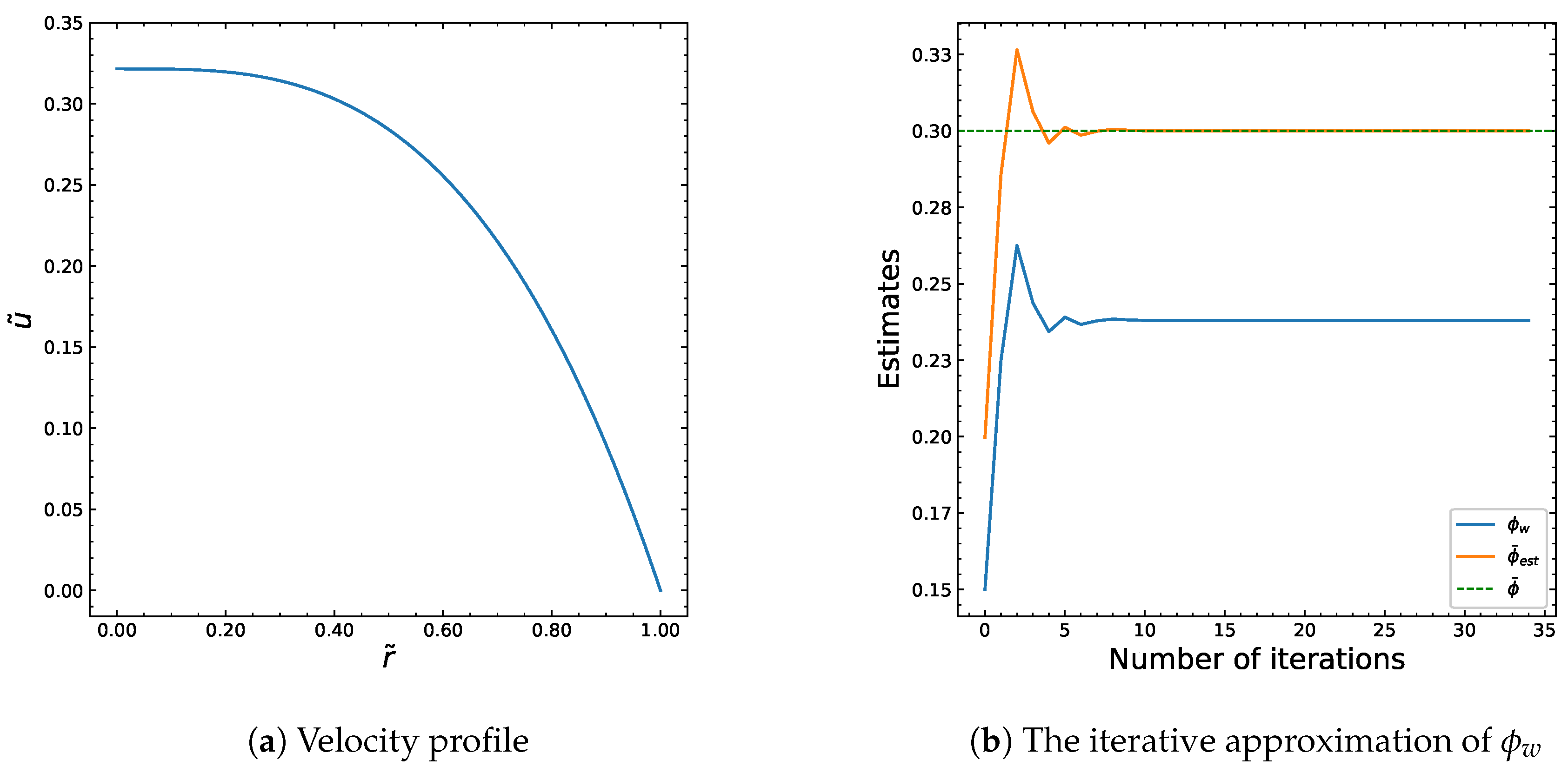
Figure 4.
The analytical and numerical solutions of particle volume fraction distribution for different .
Figure 4.
The analytical and numerical solutions of particle volume fraction distribution for different .
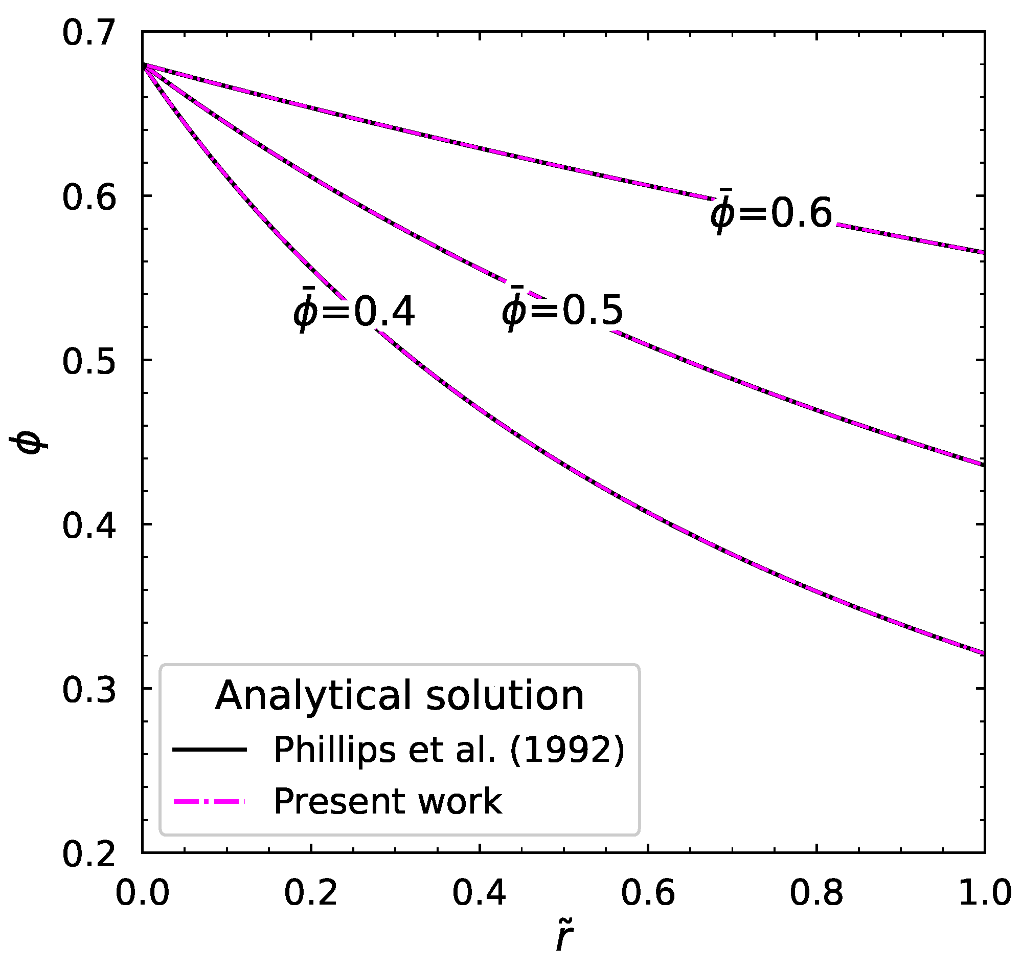
Figure 5.
The analytical and numerical solutions of particle volume fraction distribution for different power-law index n.
Figure 5.
The analytical and numerical solutions of particle volume fraction distribution for different power-law index n.
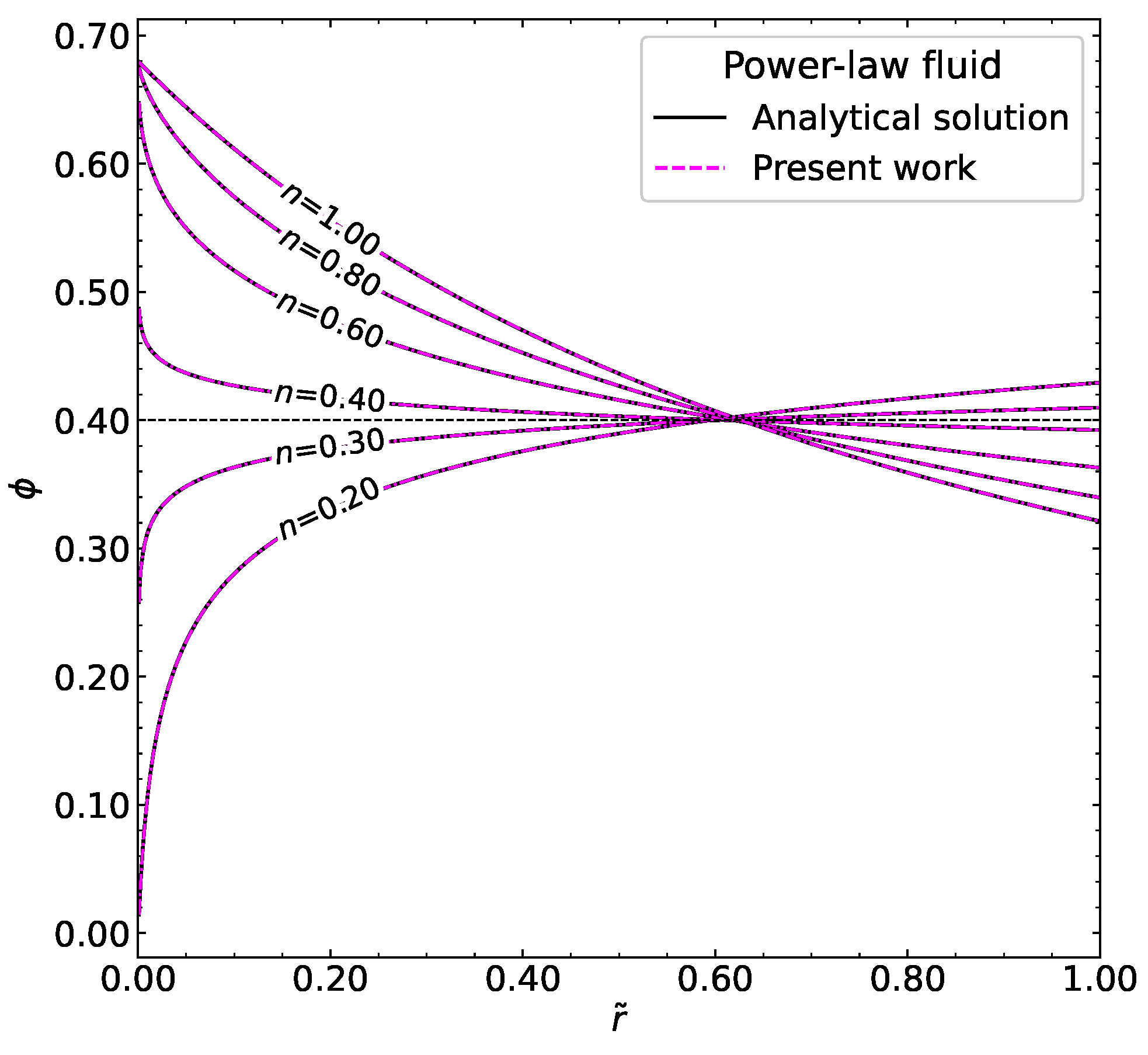
Figure 6.
The velocity and concentration profiles using various relative viscosity models.
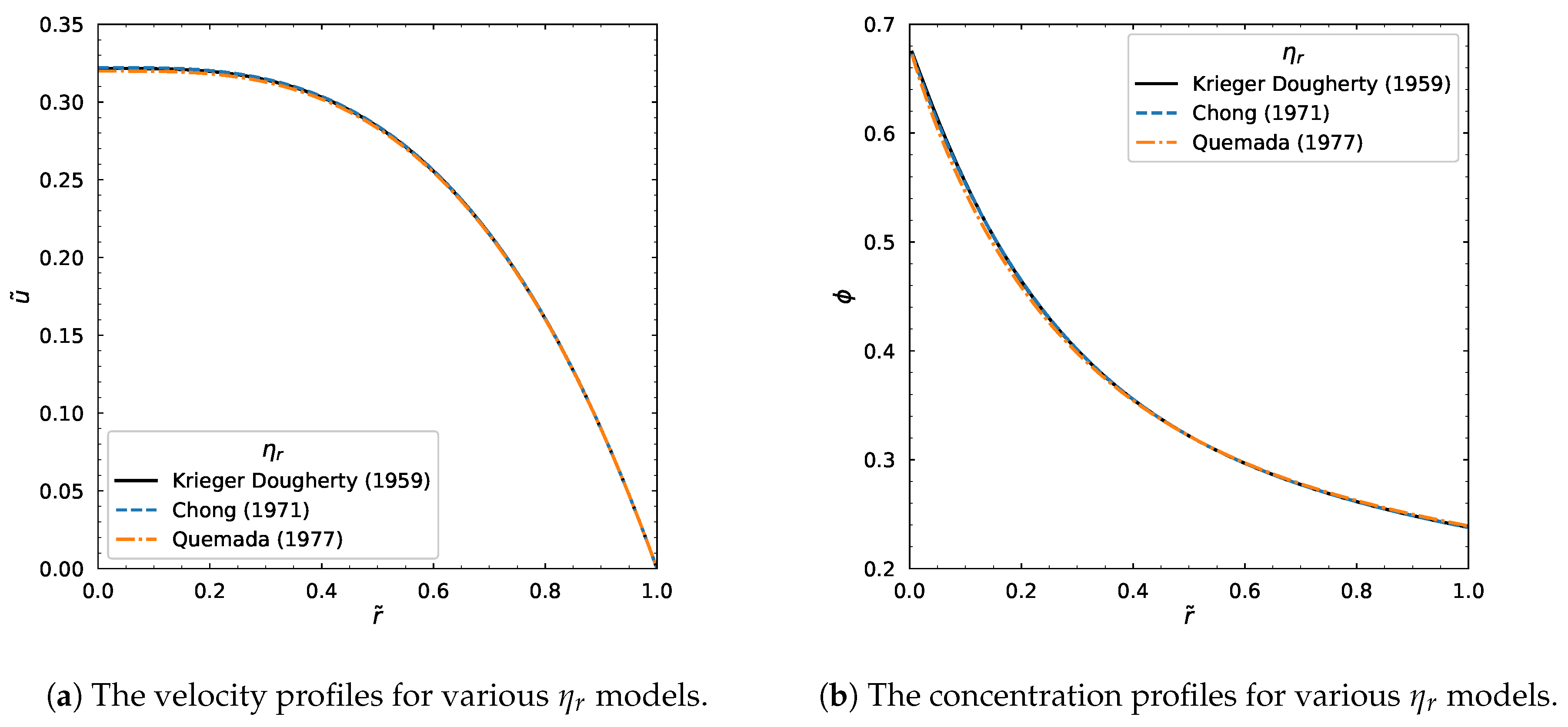
Figure 7.
Influence of . Input values used for the simulation: R = 0.01 m, = 0.68, = 0.66, = 100 Pa·s, = 1400 Pa·s, = 1.6 s, a = 1.25, n = 0.5, = 0.6 MPa/m
Figure 7.
Influence of . Input values used for the simulation: R = 0.01 m, = 0.68, = 0.66, = 100 Pa·s, = 1400 Pa·s, = 1.6 s, a = 1.25, n = 0.5, = 0.6 MPa/m
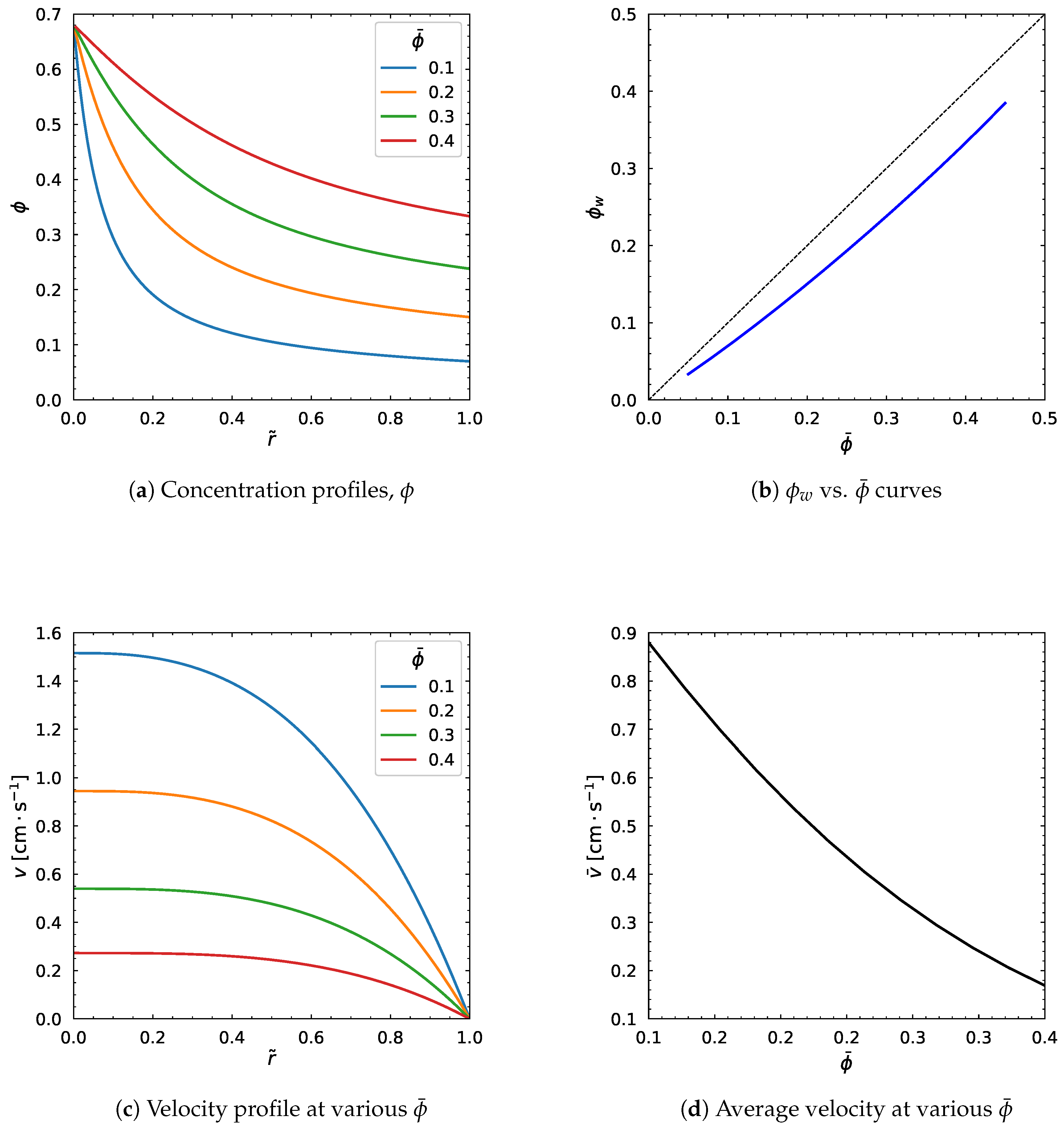
Figure 8.
Influence of pressure gradient, . Input values used for the simulation: R = 0.01 m, = 0.68, = 0.66, = 100 Pa·s, = 1400 Pa·s, = 1.6 s, a = 1.25, n = 0.5, = 0.30
Figure 8.
Influence of pressure gradient, . Input values used for the simulation: R = 0.01 m, = 0.68, = 0.66, = 100 Pa·s, = 1400 Pa·s, = 1.6 s, a = 1.25, n = 0.5, = 0.30
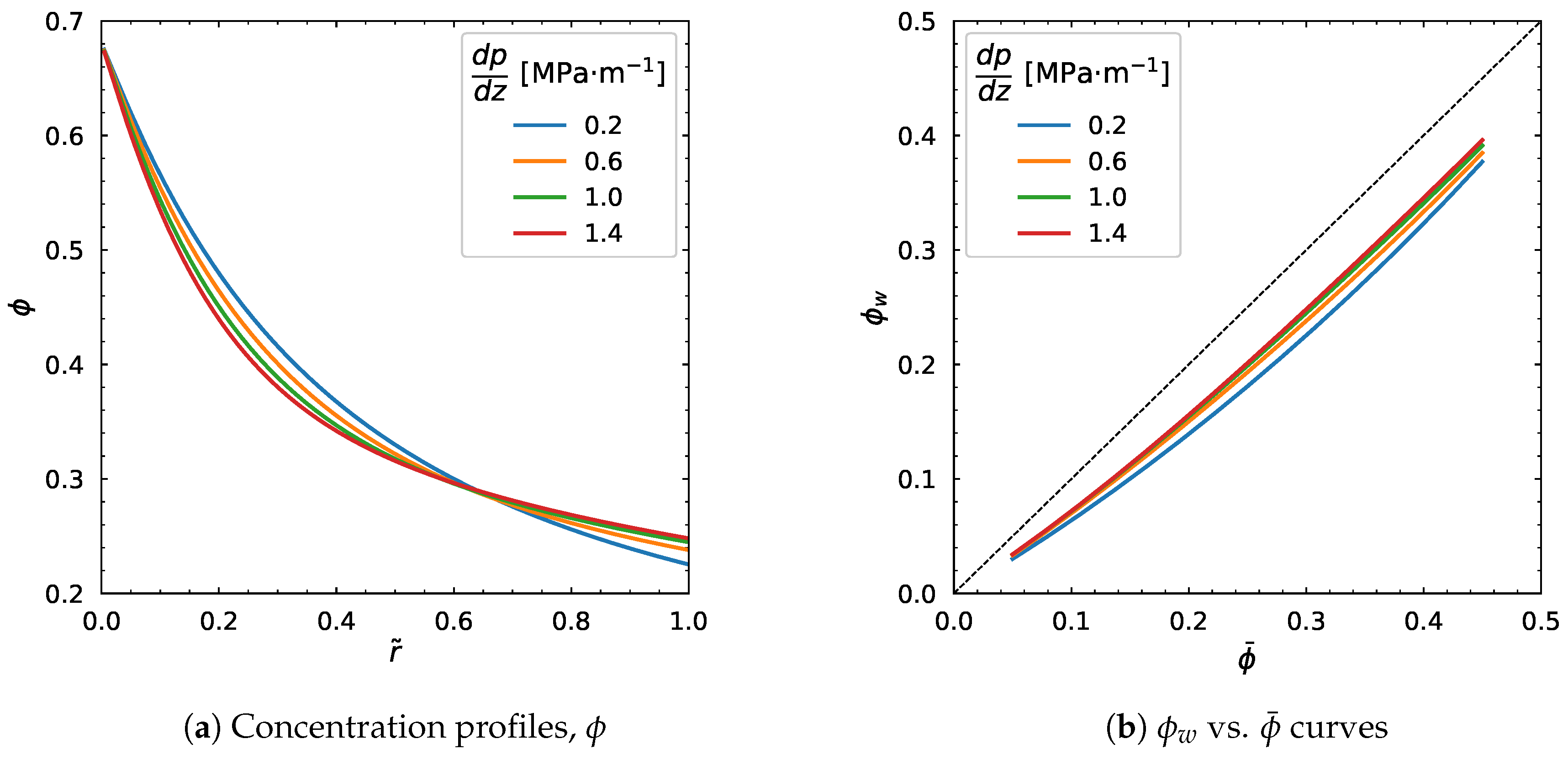
Figure 9.
Influence of pressure gradient, . Input values used for the simulation: R = 0.01 m, = 0.68, = 0.66, = 100 Pa·s, = 1400 Pa·s, = 1.6 s, a = 1.25, n = 0.5, = 0.30
Figure 9.
Influence of pressure gradient, . Input values used for the simulation: R = 0.01 m, = 0.68, = 0.66, = 100 Pa·s, = 1400 Pa·s, = 1.6 s, a = 1.25, n = 0.5, = 0.30
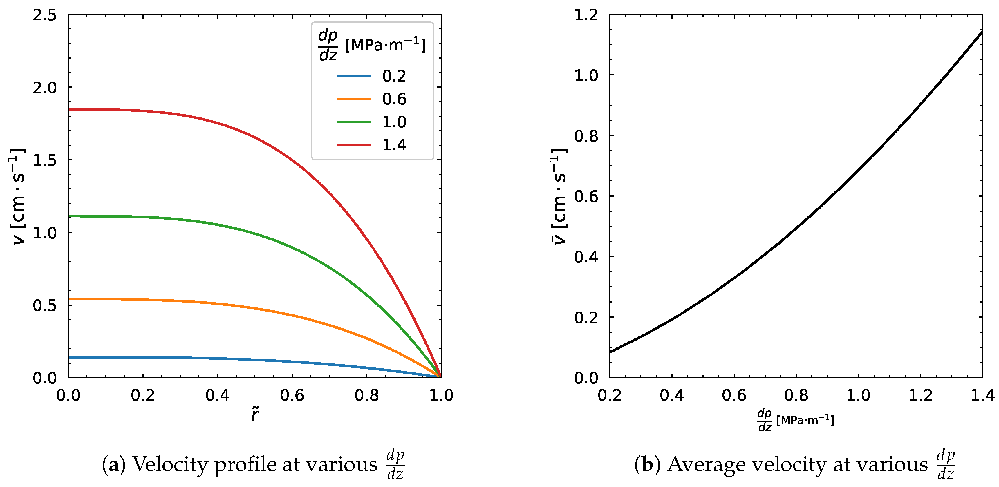
Figure 10.
Influence of . Input values used for the simulation: R = 0.01 m, = 0.68, = 0.66, = 1400 Pa·s, = 1.6 s, a = 1.25, n = 0.5, = 0.6 MPa/m, = 0.30
Figure 10.
Influence of . Input values used for the simulation: R = 0.01 m, = 0.68, = 0.66, = 1400 Pa·s, = 1.6 s, a = 1.25, n = 0.5, = 0.6 MPa/m, = 0.30
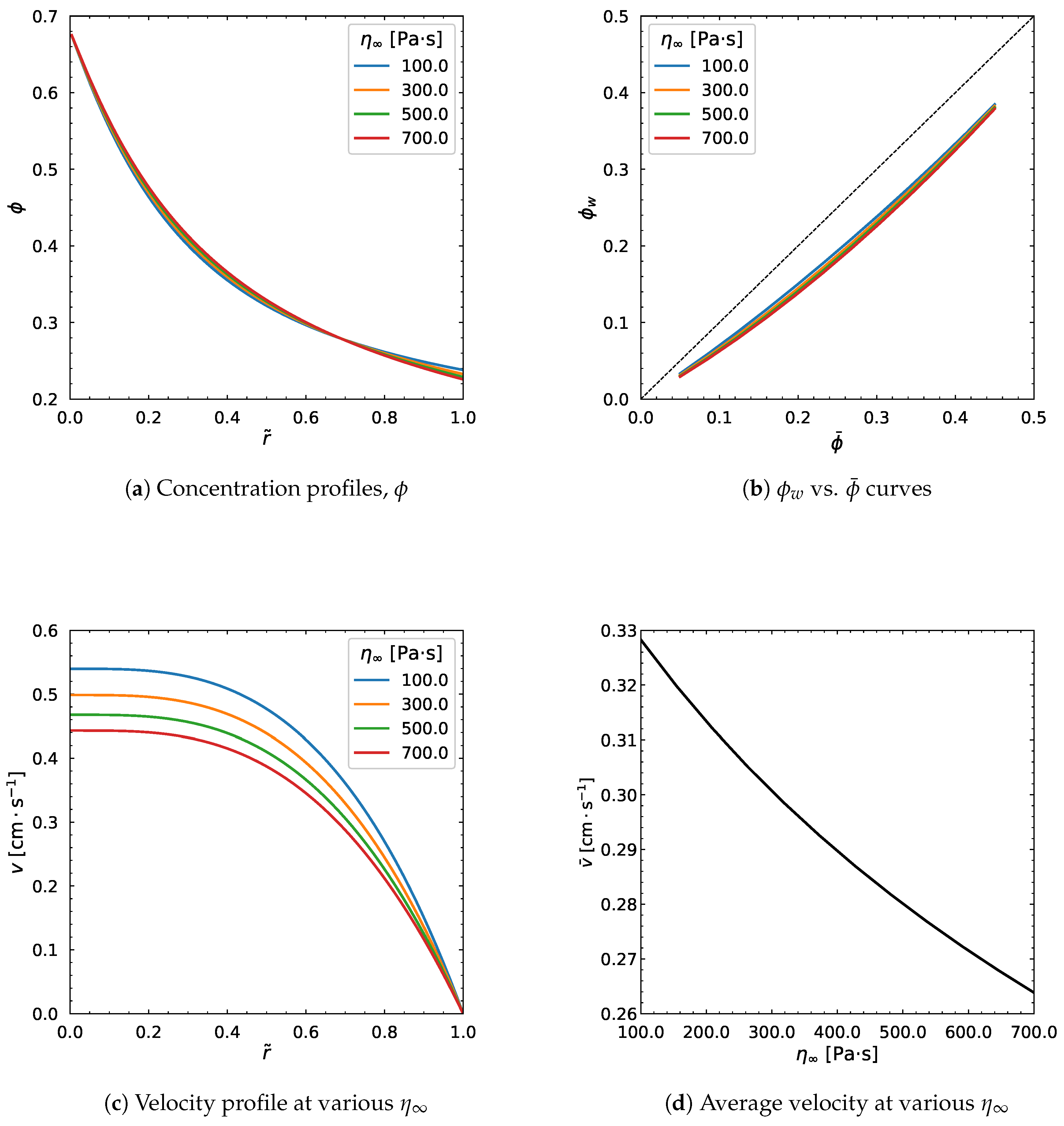
Figure 11.
Influence of . Input values used for the simulation: R = 0.01 m, = 0.68, = 0.66, = 100 Pa·s, = 1.6 s, a = 1.25, n = 0.5, = 0.6 MPa/m, = 0.30
Figure 11.
Influence of . Input values used for the simulation: R = 0.01 m, = 0.68, = 0.66, = 100 Pa·s, = 1.6 s, a = 1.25, n = 0.5, = 0.6 MPa/m, = 0.30
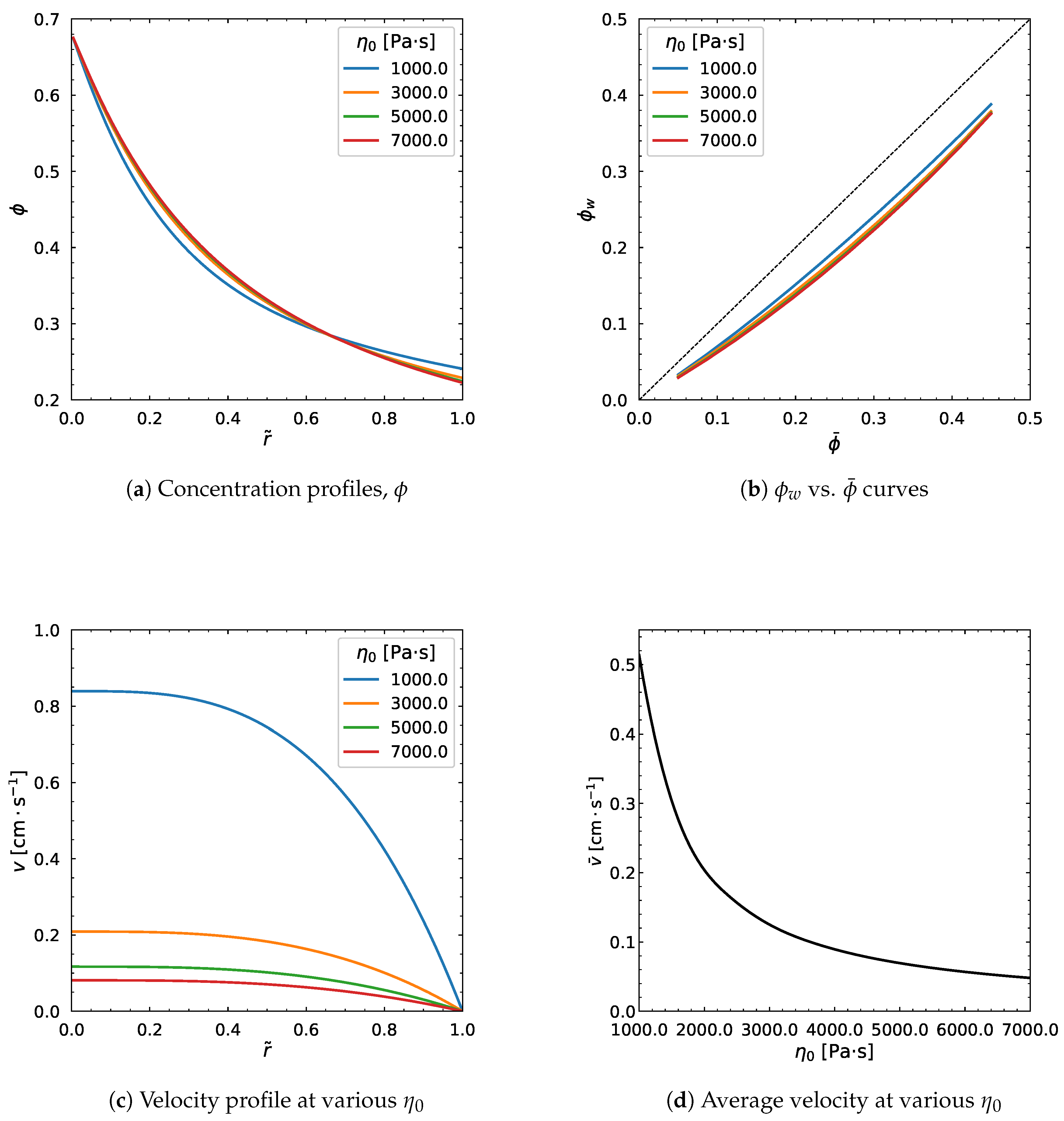
Figure 12.
Influence of a. Input values used for the simulation: R = 0.01 m, = 0.68, = 0.66, = 100 Pa·s, = 1400 Pa·s, = 1.6 s, n = 0.5, = 0.6 MPa/m, = 0.30
Figure 12.
Influence of a. Input values used for the simulation: R = 0.01 m, = 0.68, = 0.66, = 100 Pa·s, = 1400 Pa·s, = 1.6 s, n = 0.5, = 0.6 MPa/m, = 0.30
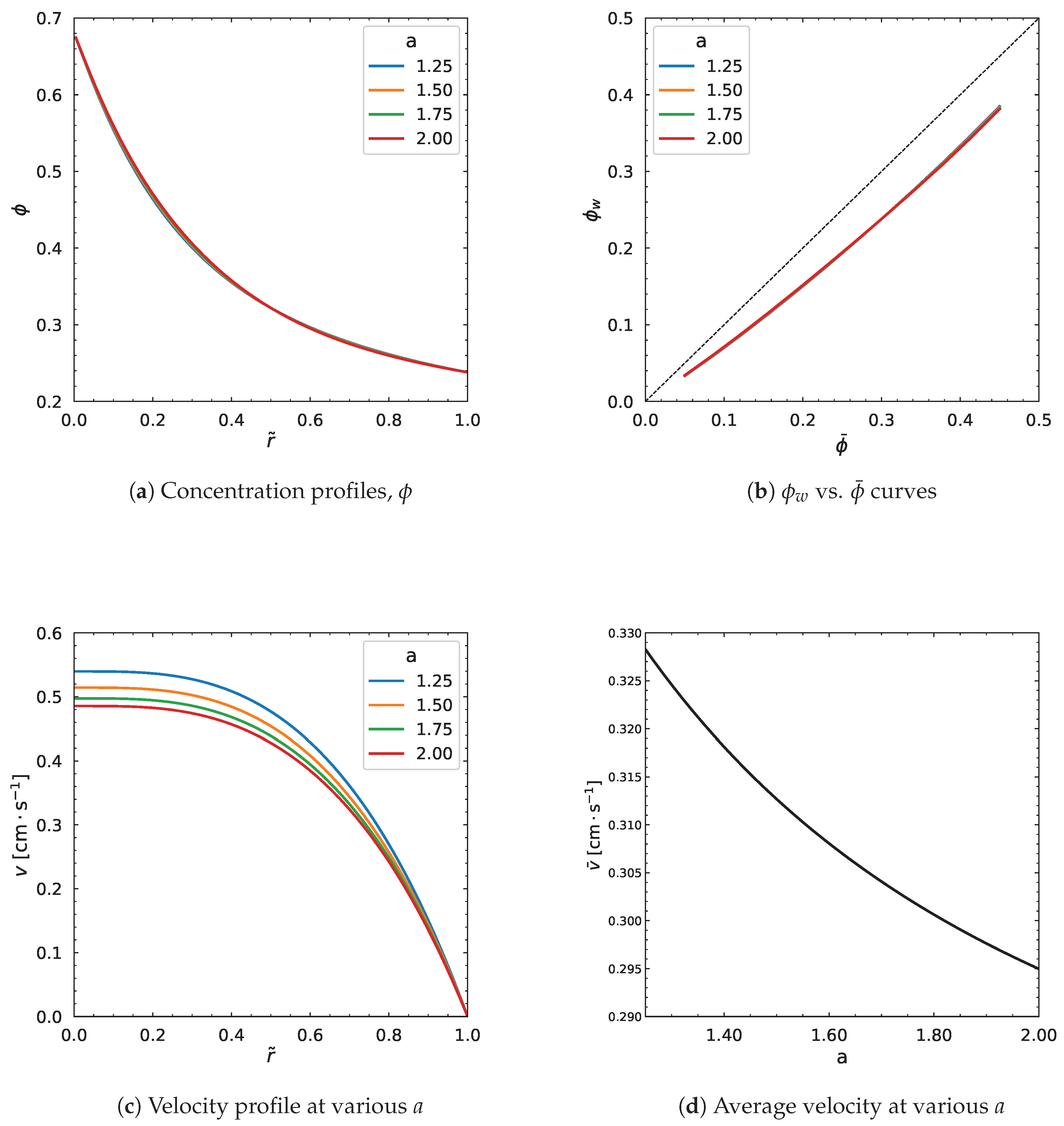
Figure 13.
Influence of . Input values used for the simulation: R = 0.01 m, = 0.68, = 0.66, = 100 Pa·s, = 1400 Pa·s, a = 1.25, n = 0.5, = 0.6 MPa/m, = 0.30
Figure 13.
Influence of . Input values used for the simulation: R = 0.01 m, = 0.68, = 0.66, = 100 Pa·s, = 1400 Pa·s, a = 1.25, n = 0.5, = 0.6 MPa/m, = 0.30
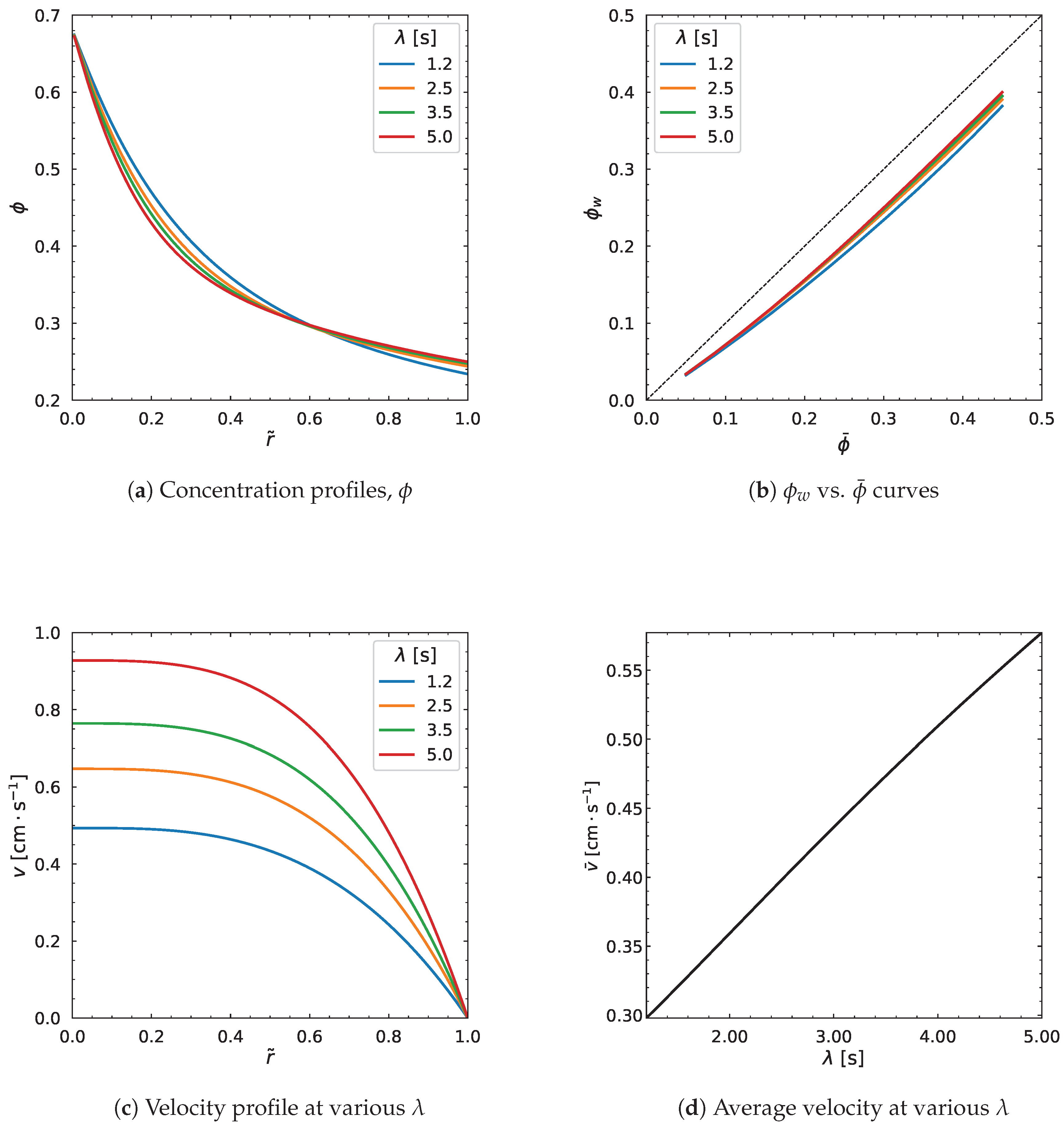
Figure 14.
Influence of n. Input values used for the simulation: R = 0.01 m, = 0.68, = 0.66, = 100 Pa·s, = 1400 Pa·s, = 1.6 s, a = 1.25, = 0.6 MPa/m, = 0.30
Figure 14.
Influence of n. Input values used for the simulation: R = 0.01 m, = 0.68, = 0.66, = 100 Pa·s, = 1400 Pa·s, = 1.6 s, a = 1.25, = 0.6 MPa/m, = 0.30
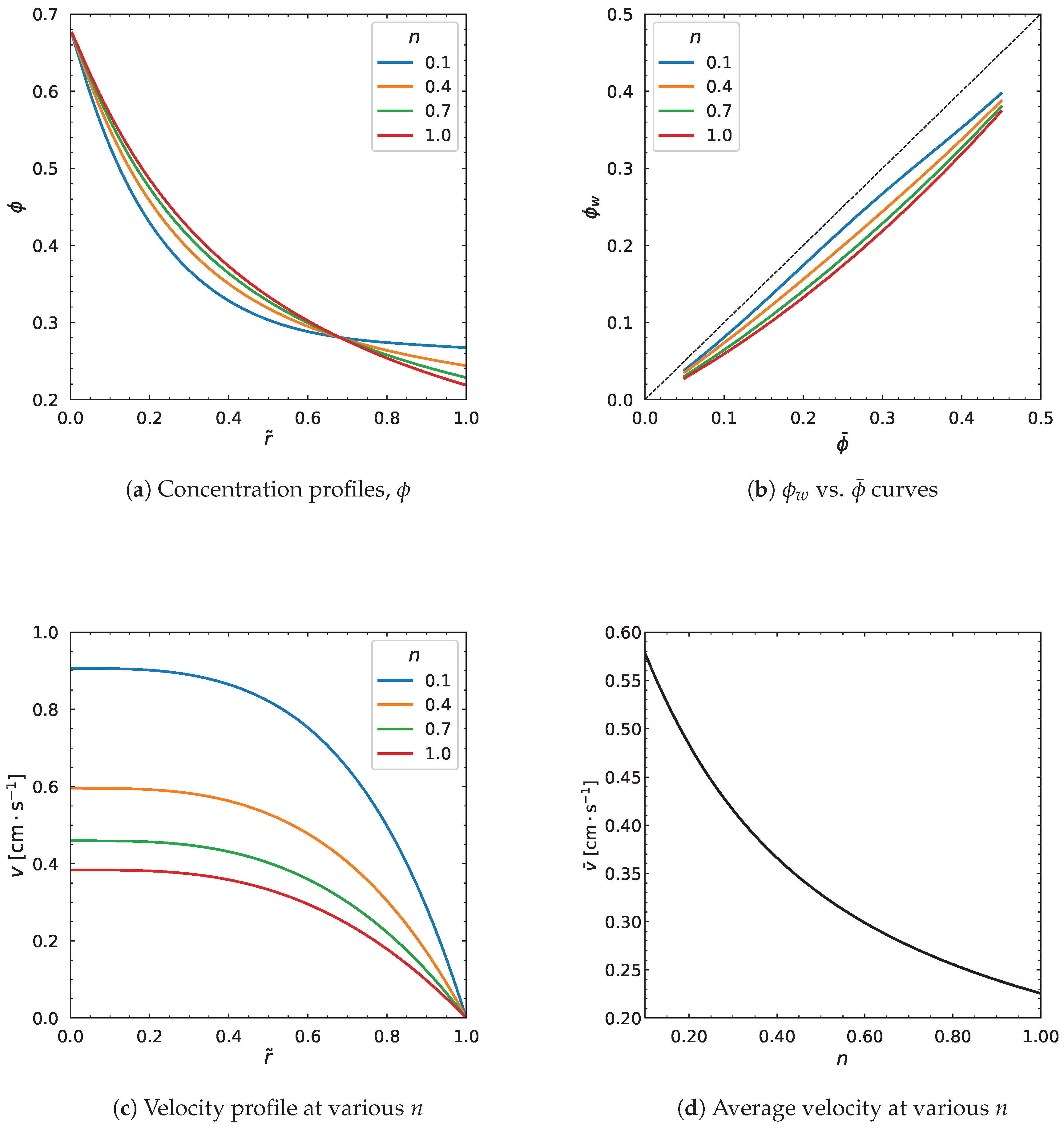
Figure 15.
Influence of parameter. Input values used for the simulation: R = 0.01 m, = 0.68, = 100 Pa·s, = 1400 Pa·s, = 1.6 s, a = 1.25, n = 0.5, = 0.6 MPa/m, = 0.30
Figure 15.
Influence of parameter. Input values used for the simulation: R = 0.01 m, = 0.68, = 100 Pa·s, = 1400 Pa·s, = 1.6 s, a = 1.25, n = 0.5, = 0.6 MPa/m, = 0.30
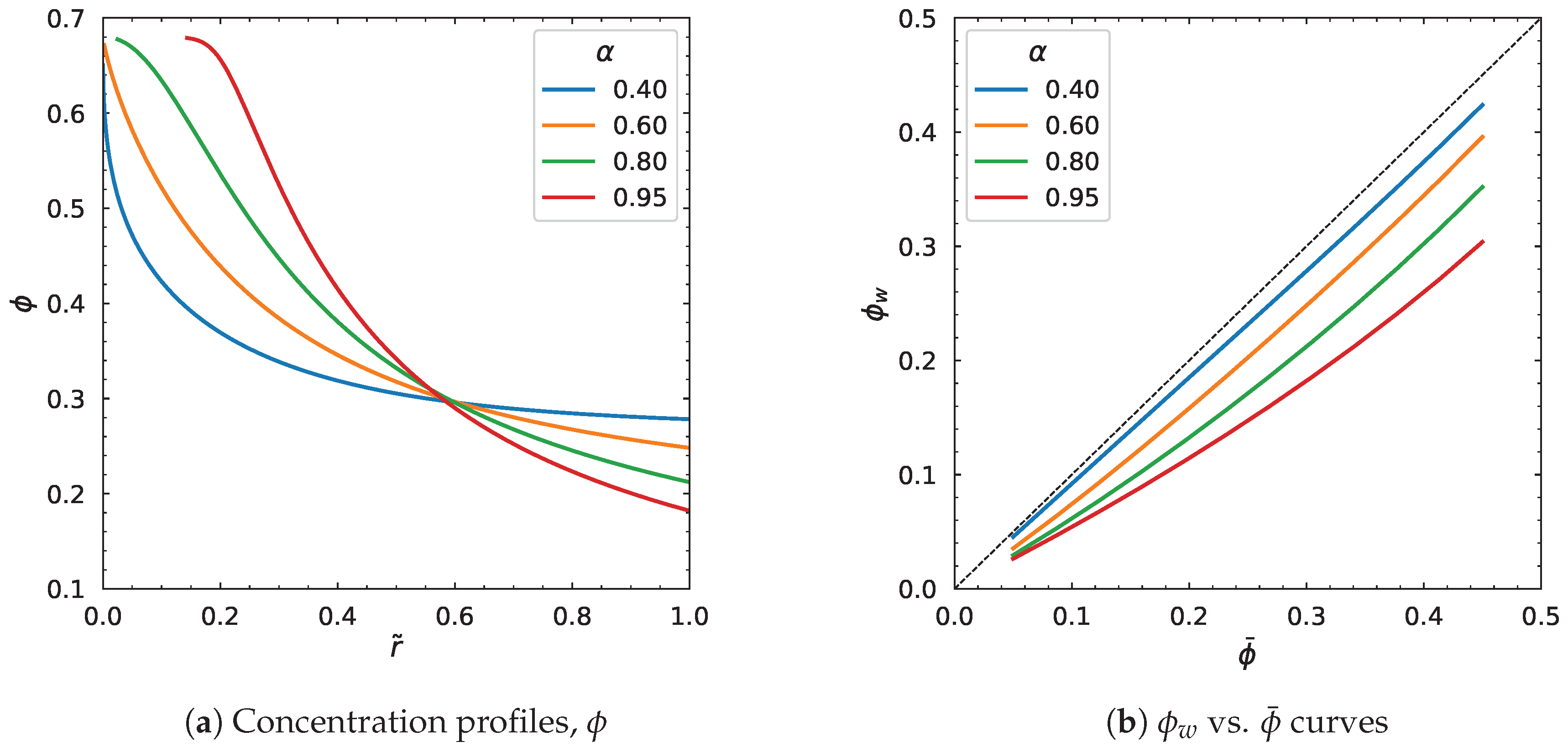
Figure 16.
Influence of parameter. Input values used for the simulation: R = 0.01 m, = 0.68, = 100 Pa·s, = 1400 Pa·s, = 1.6 s, a = 1.25, n = 0.5, = 0.6 MPa/m, = 0.30
Figure 16.
Influence of parameter. Input values used for the simulation: R = 0.01 m, = 0.68, = 100 Pa·s, = 1400 Pa·s, = 1.6 s, a = 1.25, n = 0.5, = 0.6 MPa/m, = 0.30
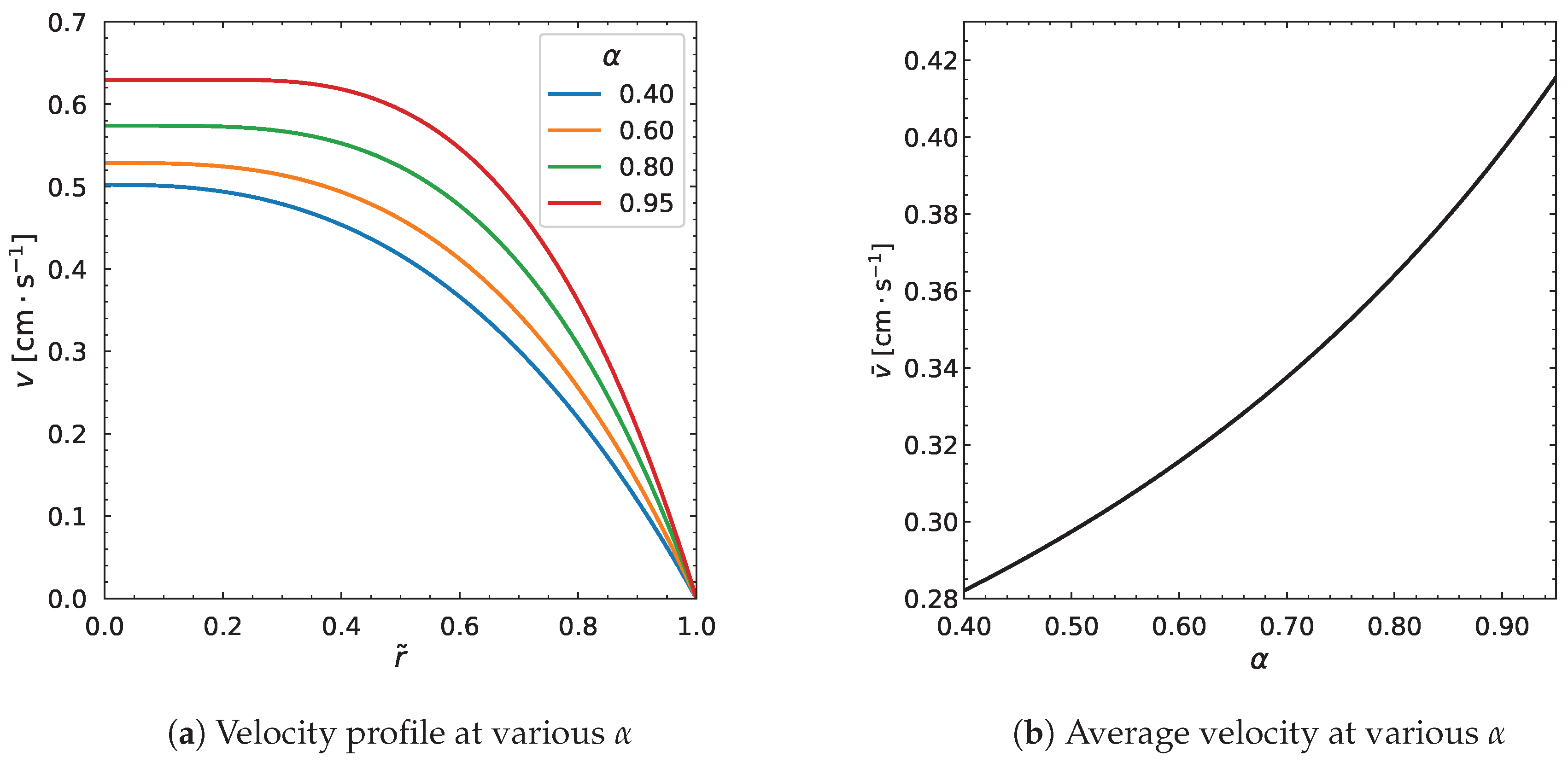

Table 1.
Constant parameters.
| Parameters | (Pa·s) | (Pa·s) | a | (s) | n | (MPa/m) | R (m) | |||
| 1400 | 100 | 1.25 | 1.6 | 0.5 | 0.6 | 0.01 | 0.68 | 0.66 | 0.3 |
Disclaimer/Publisher’s Note: The statements, opinions and data contained in all publications are solely those of the individual author(s) and contributor(s) and not of MDPI and/or the editor(s). MDPI and/or the editor(s) disclaim responsibility for any injury to people or property resulting from any ideas, methods, instructions or products referred to in the content. |
© 2025 by the authors. Licensee MDPI, Basel, Switzerland. This article is an open access article distributed under the terms and conditions of the Creative Commons Attribution (CC BY) license (http://creativecommons.org/licenses/by/4.0/).
Copyright: This open access article is published under a Creative Commons CC BY 4.0 license, which permit the free download, distribution, and reuse, provided that the author and preprint are cited in any reuse.


