
Submitted:
05 December 2024
Posted:
05 December 2024
You are already at the latest version
Abstract
This paper presents a thorough guide to simulating jet grouting using the Moving Particle Semi-Implicit (MPS) method for numerical analysis and Computer-Aided Engineering (CAE) for model development. It addresses the shortcomings of previous jet grouting simulation studies, which often lacked clear and comprehensive guidelines, by providing a detailed step-by-step approach. The key aspects of the simulation that define and shape the output of real-world jet grouting technology, such as jet grouting spray settings and material parameter configurations, are validated against benchmark experimental data. The previously challenging task of accurately determining material parameters for soil when modeled as a Bingham fluid bi-viscosity model, is simplified into a universal guideline that can be easily applied to any soil type with known unconfined compressive strength. Finally, the reliability of the jet grouting simulation is confirmed by comparing the simulation results with benchmark experimental data under similar conditions, demonstrating the robustness and accuracy of the proposed method.
Keywords:
jet grouting technology
; numerical simulation
; bingham fluid bi-viscosity model
; moving particle semi-implicit method
; simulation guidelines
1. Introduction
Simulation studies are effective research tools for the development of projects that are either too challenging, risky, or expensive to carry out in real-world scenarios. One such challenging and expensive project is jet grouting technology, which has made significant advancements since its development in the early 1970s primarily through trial and errors methods. Despite these advancements, the evaluation of jet grouting technology remains largely dependent on traditional or empirical methods [1]. Typically, jet grouting evaluation focuses on parameters such as the size and strength of the soilcrete formed, with formation of the column diameter being the most common evaluating parameter. Even in modern times, methods for confirming the diameter, such as real-time acoustic monitoring, continue to dominate the evaluation process of jet grouting technology. Thus, simulation studies to reproduce the entire jet grouting process have been proposed as an effective evaluation approach to overcome the limitations of these conventional methods [2,3,4].
Among them, the simulation and evaluation of the jet grouting technology by Moving Particle Semi-Implicit (MPS) method in combination with Computer-Aided Engineering (CAE) has been progressed with the successful formation of the jet grout column [2,3,4]. And, like all other simulation studies, the accuracy of overall jet grouting simulation depends on the accurate modeling of the jet grouting setup and ground model. However, modeling the jet grouting process itself has proven to be a complicated task, primarily due to the difficulty in accurately representing the behavior of the ground material during grouting. In geotechnical engineering, soil is often modeled as a Bingham fluid, which provides a reasonable approximation of soil behavior under various conditions. However, the challenge arises when representing the initial solid state of the ground before it undergoes the jet grouting process. To address this, the soil is assumed to behave as a Bingham fluid bi-viscosity model during the jet grouting simulation. But the material parameter determination for this model is difficult and can only be achieved through the reverse parameter fitting by unconfined compression test simulation. Despite this, the overall jet grouting simulation approach has led to successful simulations, such as the formation of the soilcrete [2,3,4] and the recreation of the mud discharge phenomenon [3], the authenticity and accuracy of these simulations remains questionable. The authenticity of the simulation results is further doubted by the lack of a clear methodology to validate simulation results. The only validation method available involves comparing the simulated soilcrete shape and diameter with the real-world soilcrete dimension when both are carried out under similar grouting conditions.
Shakya and Inazumi [5] proposed a general guideline for determining material parameters of soil using reverse parameter fitting through simulations of unconfined compression tests. While their approach is a step forward, and the guideline is ambiguous and incomplete whenever a new soil sample was used. It required complete repeat of the trial-and-error simulation to determine the material parameters of new soil sample. This process is both time-consuming and cumbersome, highlighting the need for a more streamlined and reliable method for soil parameter determination in jet grouting simulations.
The objective of this paper is to provide a comprehensive, step-by-step guideline for simulating jet grouting technology using MPS-CAE analysis. It will focus on the key steps of accurate material parameters setting and recreating jet grout spraying settings required for the jet grouting simulation. The limitations of previous studies concerning material parameter settings and jet grouting output results will be addressed. A clearer and more efficient guideline for determining material parameters for soils subjected to the Bingham fluid bi-viscosity model rheology, that can be easily applied to any soil type with known unconfined compressive strength will be proposed after verification. Lastly, this paper will verify the jet grouting simulation result with the experimental benchmark data to claim the authenticity of the jet grouting simulation approach.
2. Methodology
The optimization of the jet grouting simulation by MPS-CAE technology includes numerous distinct operations. Figure 1 shows the progressive stepwise tasks that are required to be achieved for the numerical analysis of jet grouting technology.
2.1. Modelling
The modeling of the analysis ground and jet grouting setup is carried out using Computer-Aided Engineering (CAE) technology. As the name suggests, CAE is a broad term that refers to the group of technologies used to simulate and analyze complex engineering systems, while adjusting for the site-specific conditions. It is achieved using prototypes and models created with Computer-Aided Design (CAD) software [6,7,8]. These tools enable the analysis and visualization of complex simulations by utilizing detailed representative prototypes and models. During the modeling phase, there are two key consideration factors in order to create an optimal model for jet grouting simulation. Firstly, the size of the prototype should be appropriate to ensure that the calculation points are sufficiently numerous for an accurate simulation but not large to incur exponential calculation load. If the prototype is too small or too large, the simulation’s accuracy and efficiency may be compromised. Next is the modeling of the entire setup required for analysis, which includes the ground model and the jet grouting equipment. While the size of ground model is scaled down, the jet grouting equipment is simplified by the single jet grouting string to illustrate the positioning, drilling, and jet grout spraying procedures. Figure 2 shows the scaled down ground model and jet grouting setup used for the study.
2.2. Simulation Setting
In this step, two separate but simultaneous settings must be established to correctly represent the actual construction process. The first is the jet grouting mechanism or specification settings, which are designed to accurately replicate the physical processes involved in jet grouting technology. This involves the physical notions of the installation of the jet grouting equipment on the target ground, the digging process to reach the desired depth, and the initiation of the jet grout spray to create the soilcrete. Among these processes, the jet grouting spray is the most crucial component where settings of the key parameters such as grout pressure, spray volume, grouting duration, and grouting zone must be meticulously conducted to match the actual construction procedure to ensure accuracy. However, this setup cannot be implemented directly and must be recreated by calculating the flow rate at each time frame using the Bernoulli’s equation and the Volumetric Flow Rate equation, as defined by Equations (1) and (2).
where P is the dynamic pressure, is the density of the jetted material, v is the jet velocity, Q is the Amount of jet grout, and A is the cross-sectional area of nozzle.
Next, input parameters settings that consists of calculation settings and material parameter settings must be conducted. The calculation parameter settings, such as the calculation method, time increment for the analysis, and the size of calculation points, are essential for ensuring the efficiency of the numerical analysis. Meanwhile, material parameter settings are crucial for accurately representing the materials involved in the process. In this setting, the precise properties of the key elements—water, cement grout, and soil—must be inputted to ensure that their rheological behavior is accurately replicated in the analysis. This ensures that the interactions between these materials are modeled realistically, reflecting their actual behavior in the jet grouting process.
2.3. Numerical Simulation
Moving Particle Semi-Implicit (MPS) method is the numerical analysis method that was used to analyze this study. It is one of the particle methods in which participating elements are assumed to be composed of numerous particles. These particles act as the calculation points that move along with the physical quantity in a lagrangian manner. Equations 3 and 4 are the governing equations for these numerical methods and are called mass conservation law for incompressible flow and Navier’s stroke law respectively [9,10].
where is the density of the fluid, is the velocity vector of fluid, is the rate of change in velocity vector, is the rate of change in density, is the fluid pressure, is the kinematic viscosity coefficient, and is the gravity vector.
3. Analysis Condition and Material Parameter
Table 1 shows the analysis conditions for the study representing actual experimental jet grouting conditions that need to be recreated in the numerical simulation of jet grouting technology.
3.1. Rheology Fittings
Rheology refers to the study of fluid behavior and its flow characteristics. Fluids are broadly classified into Newtonian fluid and non-Newtonian fluid. Newtonian fluids follow Newton’s law of viscosity, exhibit a linear relationship between shear stress and shear strain, and their viscosity remains constant, irrespective of the applied shear stress. A prime example of a Newtonian fluid is water, which is one of the key elements in jet grouting simulations.
Meanwhile, Bingham fluid is one of the non-Newtonian fluids that remain stationary until the applied shear stress exceeds their yield stress and will flow like a viscous fluid after crossing the threshold stress. Above the yield stress, it exhibits a linear relationship between shear stress and shear rate and the flow behavior can be described by a linear equation similar to that of Newtonian fluids, but with an added yield stress term. In jet grouting technology, the grout—a mixture of water and cementitious material—exhibits sufficient fluidity while being viscous in nature, making it a classic example of a Bingham fluid. The flow behavior of a Bingham fluid can be mathematically expressed by Equation (5).
where is the shear stress, is the yield stress, is the plastic viscosity, and is the shear rate.
As for the remaining soil element, it is widely accepted to represent it by Bingham fluid in simulation [11,12,13,14,15] due to its defining characteristics of yield stress and viscosity [16]. However, the soil in question will initially exist in a solid state and cannot be accurately classified as a true fluid. Hence, it creates a challenge in analyzing the behavior of a soil in its rigid state, where the shear stress does not exceed the yield stress [17]. Since the accuracy of simulations hinges on employing an appropriate rheological model, a modified Bingham fluid approach is required to capture the complex rheological behavior of the soil [18,19]. To address this limitation, the Bingham fluid bi-viscosity model is employed, which accounts for the dual nature of the soil, treating it as a viscous-plastic fluid when in a fluid state and as a highly viscous material when in a rigid state [20]. Equations 6 and 7 define the apparent viscosity of Bingham fluid bi-viscosity model in a fluid state and rigid state respectively. Figure 3 shows the comparison on schematic diagrams of Newtonian fluid, Bingham fluid model and bi-viscosity Bingham model.
where is the pressure, is the plastic viscosity, is the yield value, is an average shear velocity and is a yield criterion of the fluid and rigid states.
The equation for the yield criterion of fluid and rigid state is expressed by Equation (8) as
where Cy is a yield parameter.
Here, the apparent viscosity in a rigid state is the viscosity that was introduced to regularize the Bingham model into the bi-viscosity model, and instead of discussing this dummy viscosity, is often represented by the dimensionless parameter ϵ, which is the generally defined as the ratio of plastic viscosity () and dummy viscosity (
) [21]. This approach is justified from the perspective of physical meaning where the introduction of a large but finite viscosity at very small strain rate is more realistic than labelling simple dummy viscosity [22]. Meanwhile, this approach is also justified mathematically since this allows for smoothing of a non-differentiable minimization problem [23].
This regulatory parameter ε when considered as the model parameter, the critical shear rate can be derived [24] and given by Equation 9.
When the value of ε tends equal to 0, the model becomes the Bingham model [25]. When the value of ε tends equal to 1, then model becomes the Newtonian model.
From the two different equations for the yield criterion, we can determine the Equation 10 between the regulatory parameter and yield parameter.
It indicates that the viscosity of the Bingham fluid bi-viscosity model is the function of yield parameter.
3.2. Material Parameter
Water, as a standard Newtonian fluid, has well-established rheological properties that remain constant under specific temperature and pressure conditions. For materials like grout, rheological properties such as plastic viscosity and yield stress can be measured using specialized instruments like B-type viscometers and rheometers. These devices are designed to assess the rheology of fluids with adequate fluidity. Figure 4 and Figure 5 illustrate the typical examples of a B-type viscometer and a rheometer, respectively.
The B-type viscometer operates by attaching spindles of varying sizes, which are submerged in the fluid and rotated to measure its rheological properties [26]. The torque generated on the spindle's rotating shaft quantifies the fluid’s resistance to flow, reflecting its rheological behavior. Similarly, a rheometer functions on the same principle but incorporates a more advanced design and additional features. In this device, a thin layer of fluid is applied to a base plate, and the spindle comes into contact with the fluid. The spindle’s rotation enables the measurement of more complex rheological properties, along with real-time monitoring during the process [27,28,29].
Direct measurement of rheological data for soil is challenging due to its insufficient fluidity. Soil samples may not yield under testing conditions, and even if yielding occurs, the measured values are often inconsistent and unreliable. Thus, the material parameter for the soil in rigid state are determined by the reverse parameter fitting by unconfined compression test simulation [30].
3.2.1. Reverse parameter fitting for soil material parameter Setting
Shakya and Inazumi [5] have proposed a guideline for determining the material parameters of known unconfined compressive strength. The key points from the guidelines provided by Shakya and Inazumi [5] are as follows:
- The yield value is always half of the unconfined compressive strength and is applicable to all soil types.
- A yield parameter value of approximate 1/10,000 produces accurate results. Meanwhile, a yield parameter value above 1/1,000 results in the soil sample failing to retain its shape.
- A lower critical shear strain value around 2*0.00012 s-1 generates the best fitting results.
- Keeping the critical shear strain constant while varying the yield parameter and plastic viscosity did not affect the output results.
Using the guideline above, the material parameter for the soil sample of unconfined compressive strength 60 kPa was determined. Table 2 shows the material parameters of the key elements of jet grouting technology.
4. Results and Discussion
4.1. Verification of the Reverse Parameter Fittings
A soil sample with an unconfined compressive strength of 60 kPa was selected for jet grouting simulation. Since the exact material parameters of this soil were unknown, the guideline was applied for the reverse parameter fitting of this soil sample. Based on the guideline, the critical shear strain for two different soil samples was calculated to be approximately 2*0.00012 s-1, suggesting that this value might be consistent for all soil types. This assumption aligns theoretically with the Bingham fluid bi-viscosity model, which suggests that soil transitions from a rigid to a fluid state only after experiencing deformation equal to the critical shear strain. Since this deformation is relatively small compared to the deformation caused when the yield stress exceeds the yield value, it seems reasonable to assume a similar critical shear strain value for all soil types.
To test this assumption, this study studied the output stress-strain curve characteristics for different soil samples using the same critical shear strain value. Figure 6a) and 6b) illustrates the sensitivity analysis of 60 kPa soil for the different yield parameter value at the critical shear strain value of 2*0.00012 s-1. However, the output results for strength and strain did not match the benchmark sample data of 60 kPa soil. This discrepancy suggests two possibilities:
- The critical shear strain value from the guideline is not universally accurate for all soil types.
- The assumption that all soils share the same critical shear strain value may be incorrect.
To confirm that the critical shear strain value is constant for all soils, it is necessary to determine an accurate value that satisfies the Bingham fluid bi-viscosity model relationship and simultaneously generates realistic stress-strain curve characteristics when used for each soil type.
4.1.1. Determination of Representative Critical Shear Strain for all Soil Samples
Since the approximate critical shear strain value from the guideline was inaccurate for different soil samples, this study aimed to determine a more precise critical shear strain value that could represent all soil types effectively. Figure 7 presents a sensitivity analysis conducted on a random soil sample with an unconfined compressive strength of 100 kPa. The yield value and yield parameter were used as constant parameter, while plastic viscosity was adjusted to vary the critical shear strain, as per the rule of guideline [5]. The results indicate that lower critical shear strain values yield more accurate stress-strain characteristics, consistent with the guideline's predictions [5]. Table 3 details the material parameters used for this sensitivity analysis. The yield parameter was set at 0.0001, as suggested in the initial stages of the guideline. The analysis revealed that reducing the critical shear strain value increases the output strength and reduces strain value, implying that with higher plastic viscosity leads to a greater output strength and a more brittle soil response [5]. The recalculated critical shear strain values of 2*0.00018 s-1 and 2*0.000177 s-1 produced similar stress-strain characteristics, with the latter providing slightly better results. The "factor of two" in these values represents the constant value from Equation 8 of the Bingham fluid bi-viscosity model relationship. To verify this finding and prove that the critical shear strain value of 2*0.000177 s-1 may be the representative value for all soil types, this value will be tested on additional soil samples.
Figure 8 shows the simulated stress-strain curves compared to the two benchmark datasets with approximately equal unconfined compressive strengths, using the recalculated critical shear strain value of 2*0.000177 s-1. This recalculated value effectively reproduced accurate stress-strain curves for new soil samples of approximately 60 kPa unconfined compressive strength. An output strength of 61.59 kPa at a strain of 1.162% was recorded for an input plastic viscosity of 17,000 Pa.s and a yield parameter value of 0.0001.
4.1.2. Determination of Representative Yield Parameter Value for All Soil Sample
Figure 9 shows sensitivity analysis for the yield parameter compared with the Yamagata soil sample in order to determine the exact representative yield parameter value in simulation for all soil types. The critical shear strain value for each case is 2*0.000177 s-1 and the most accurate result was obtained when the yield parameter value was set as 0.0001 with the curve characteristics as shown in fig 8. In contrast, all other cases produced an approximate strength of 57 kPa at the strain value of 1.2%. Thus, it can be inferred that the best fitting material parameter for this specific soil sample are a yield parameter value of 0.0001 and critical shear strain value of 2* 0.000177 s-1.
Since the simulation study assumes the model to be composed of homogenous and uniformly sized soil particles, and the dual viscosities of the bi-viscosity model depends upon the yield parameter as defined by the Equation 10, it is recommended to adopt the parameter that yields the best-fitting result as representative material parameters. To validate this statement holds true for all soil types, further verification is required to confirm whether the output results align with these calculated values.
4.1.3. Verification of Recalculated Representative Soil Parameters
Figure 10 and Figure 11 show the verification simulation for soil samples 1 and 2 respectively, used as benchmark dataset by Shakya and Inazumi [5]. These simulations compare the previously generated stress-strain curves with the newly obtained stress-strain characteristics, which were derived using recalculated representative yield parameters and critical shear strain values that are applicable to all soil samples. Table 4 highlights the changes in simulation parameter values for comparison.
The limitation of the old reverse parameter fitting simulation was the requirement to repeat the whole guideline from scratch to determine the material parameter of the new soil sample. This made the guideline incomplete and ambiguous, particularly for soil samples with unconfined compressive strengths different from samples 1 and 2. In this study, representative critical shear strain and yield parameter values were determined from a 61.55 kPa soil sample and a 100 kPa soil sample, respectively. These parameters were then tested on soil samples with unconfined compressive strengths of 25.8 kPa and 39.5 kPa, generated accurate results. However, the method still required verification for soil strengths higher than those used to establish the representative values. Figure 12 shows the result of verification simulation conducted on higher-strength soil samples. For soil sample 3, with an unconfined compressive strength of 366.19 kPa, the simulated yield strength was 364.16 kPa, demonstrating excellent agreement. Thus, after the successful verification with the five different soil samples of different range of strength, it can be confirmed that the representative yield parameter and critical shear strain is applicable for all soil types.
4.2. Verification of Jet Grouting Simulation
The verification of the jet grouting technology presents a challenge due to the lack of direct and effective confirmation methods. In real-world applications, direct visualization of soilcrete is impossible without damaging it. Traditionally, the primary method for verification of jet grouting technology is confirming the diameter of the grouted column. Strength verification, on the other hand, is less common and typically involves extracting core samples for unconfined compression testing. However, this approach is generally limited to prototypes only due to its destructive nature. Meanwhile, simulation studies as the evaluation of jet grouting are primarily focused on deformation analysis or prediction of diameter and strength, rather than the verification of overall construction. The size of soilcrete on field if matches with the predicted studies, then the jet grouting technology is considered as verified.
Under such scenarios, the verification of the overall jet grouting simulations should be based on the available data. The formation of the jet grout column depends on several factors, including jet pressure at the nozzle, soil characteristics, grouting parameters, grout properties, and the selected method of jet grouting. Since no direct correlation has been established for these complex variables, the simulation results must be validated by comparing the predicted column diameters with experimental outcomes under identical grouting conditions. For the analysis studies, literature reviews [31,32] indicate that analytical models are typically validated against experimental results, such as those involving water jet tests. The construction specifications for this jet grouting simulation were matched with the jet grouting spray conditions for benchmark data [2,3]. Comparisons between the horizontal distances traveled by experimental and analytical jets revealed a consistent trend, confirming the accuracy of the jet spray settings used in the simulation. Figure 13 illustrates the relationship between jet distance and flow pressure for the applied construction specification. For the same jet grouting condition, it was reported to have the soilcrete formation of an approximate 1 m diameter [2].
Figure 14 and Figure 15 illustrate the soilcrete formation from different perspectives in this simulation study. Figure 14 provides a 360-degree view, while Figure 15 shows the top view of the maximum diameter achieved during jet grouting. The simulation resulted in a maximum diameter of 1 m and a soilcrete height of 0.79 m. Compared to the previous simulation [2], where identical jet grouting conditions were applied, these results demonstrate a significant improvement. This improvement is attributed to adjustments in the material parameters, highlighting the importance of accurate ground modeling in achieving realistic simulation outcomes.
5. Conclusions
This study provides a comprehensive guideline for MPS-CAE simulation of jet grouting technology, covering all stages from initial modeling to the final numerical analysis outputs, along with verification for each objective. A critical aspect of the simulation lies in accurately recreating the jet grouting spray settings and determining precise material parameters. While previous studies have successfully modeled jet grouting spray settings, accurately defining the material parameters of soil, which follows the rheology of a Bingham fluid but remains in a rigid state during the initial stage, has been a significant challenge. This research offers a complete framework for determining soil material parameters for the Bingham fluid bi-viscosity model, provided the unconfined compressive strength value is known. Additionally, the study validated the authenticity of the jet grouting simulation using the MPS-CAE method by comparing simulation results with experimental data under identical jet grouting conditions.
However, the study is limited in its ability to recreate realistic stress-strain curves for soils with the same unconfined compressive strength but different yielding characteristics. Since the simulation uses a homogeneous and uniformly distributed soil model for the reverse parameter fitting, it restricts the variability in output patterns. As a result, the model may not accurately represent the stress-strain characteristics of diverse soil types with the same unconfined compressive strength, potentially rasing the concern about the precision of the calculated material parameters. Meanwhile, jet grouting simulation has to rely on the traditional evaluation methods for the authentication. Future research should focus on advancing jet grouting simulation into a more robust research and evaluation tool by integrating additional correlated parameters beyond the jet grout spray settings and material parameters setting which could influence the outcomes of jet grouting technology.
Author Contributions
Conceptualization, S.I. and G.C.; methodology, S.I. and G.C.; software, S.S. and S.I.; validation, G.C. and S.I.; formal analysis, S.S. and S.I.; investigation, S.S. and Y.H.; resources, G.C. and Y.H.; data curation, S.S. and G.C.; writing—original draft preparation, S.S.; writing—review and editing, S.I.; visualization, S.I.; supervision, S.I. and G.C.; project administration, S.I.; funding acquisition, S.I. All authors have read and agreed to the published version of the manuscript.
Funding
This research received no external funding.
Data Availability Statement
The data presented in this study are available upon request from the corresponding author.
Conflicts of Interest
The authors declare no conflicts of interest.
References
- Inazumi, S.; Shakya, S. A Comprehensive Review of Sustainable Assessment and Innovation in Jet Grouting Technologies. Sustainability 2024, 16, 4113. [Google Scholar] [CrossRef]
- Inazumi, S.; Shakya, S.; Komaki, T.; Nakanishi, Y. Numerical analysis on performance of the middle-pressure jet grouting method for ground improvement. Geosciences 2021, 11, 313. [Google Scholar] [CrossRef]
- Shakya, S.; Inazumi, S.; Nontananandh, S. Potential of Computer-Aided Engineering in the Design of Ground-improvement technologies. Applied Science 2022, 12, 9675. [Google Scholar] [CrossRef]
- Shakya, S.; Inazumi, S.; Chao, K.C.; Wong, R.K.N. Innovative Design Method of Jet Grouting Systems for Sustainable Ground Improvements. Sustainability 2023, 15, 5602. [Google Scholar] [CrossRef]
- Shakya, S.; Inazumi, S. Applicability of Numerical Simulation by Particle Method to Unconfined Compression Tests on Geomaterials. Civil Engineering Journal 2024, 10, 1–19. [Google Scholar] [CrossRef]
- Chang, K.H. Product Design Modeling Using CAD/CAE: The Computer Aided Engineering Design Series; Elsevier: Amsterdam, The Netherlands, 2014. [Google Scholar]
- Hamri, O.; Léon, J.C.; Giannini, F.; Falcidieno, B. Software environment for CAD/CAE integration. Advances in Engineering Software 2010, 41, 1211–1222. [Google Scholar] [CrossRef]
- Pan, Z.; Wang, X.; Teng, R.; Cao, X. Computer-aided design-while-engineering technology in top-down modeling of mechanical product. Computers in Industry 2016, 75, 151–161. [Google Scholar] [CrossRef]
- Koshizuka, S.; Oka, Y. Moving-Particle Semi-Implicit Method for Fragmentation of Incompressible Fluid. Nuclear Science and Engineering 1996, 123, 421–434. [Google Scholar] [CrossRef]
- Kondo, M.; Koshizuka, S. Suppression of Unnatural Numerical Oscillations in the MPS Method. Transactions of the Japan Society for Computational Engineering and Science 2008, 20080015. [Google Scholar] [CrossRef]
- Marr, J. G.; Elverhøi, A.; Harbitz, C.; Imran, J.; Harff, P. Numerical simulation of mud-rich subaqueous debris flows on the glacially active margins of the Svalbard–Barents Sea. Marine Geology. [CrossRef]
- Luna, B. Q.; Remaître, A.; van Asch, T. W. J.; Malet, J.-P.; van Westen, C. J. Analysis of debris flow behavior with a one dimensional run-out model incorporating entrainment. Engineering Geology 2012, 128, 63–75. [Google Scholar] [CrossRef]
- Geertsema, M.; Hungr, O.; Schwab, J. W.; Evans, S. G. A large rockslide–debris avalanche in cohesive soil at Pink Mountain, northeastern British Columbia, Canada. Engineering Geology. [CrossRef]
- Montassar, S.; de Buhan, P. A numerical model to investigate the effects of propagating liquefied soils on structures. Computers and Geotechnics 2006, 33, 108–120. [Google Scholar] [CrossRef]
- Wachs, A. Numerical simulation of steady Bingham flow through an eccentric annular cross-section by distributed Lagrange multiplier/fictitious domain and augmented Lagrangian methods. Journal of Non-Newtonian Fluid Mechanics. [CrossRef]
- Aberqi, A.; Aboussi, W.; Benkhaldoun, F.; Bennouna, J.; Bradji, A. Homogeneous incompressible Bingham viscoplastic as a limit of bi-viscosity fluids. Journal of Elliptic and Parabolic Equations 2023, 9, 705–724. [Google Scholar] [CrossRef]
- Urano, S; Nemoto, H. Fresh concrete using flow analysis method research on evaluation of constructability of road. Shimizu Corporation Research Report 2013, 90, 55–66. [Google Scholar]
- Garrido, L.; Gainza, J.; Pereira, E. Influence of sodium silicate on the rheological behaviour of clay suspensions-Application of the ternary Bingham model. Applied Clay Science 1988, 3, 323–335. [Google Scholar] [CrossRef]
- Leonardi, C.R.; Owen, D.R.J.; and Feng, Y.T. Numerical rheometry of bulk materials using a power law fluid and the lattice Boltzmann method. Journal of Non-Newtonian Fluid Mechanics. [CrossRef]
- Shakya, S.; Inazumi, S. Ground modelling by MPS-CAE simulation under different influencing parameters, Smart Geotechnics for Smart Societies 2023, 2365-2369. [CrossRef]
- Lenci, A.; Di Federico, V. A Channel Model for Bi-viscous Fluid Flow in Fractures. Transport in Porous Media 2020, 134, 97–116. [Google Scholar] [CrossRef]
- Barnes, H.A.; Walters, K. The yield stress myth? Rheologica acta, /: 323–326. https, 1007. [Google Scholar]
- Frigaard, I.; Nouar, C. On the usage of viscosity regularisation methods for visco-plastic fluid flow computation. Journal of non-newtonian fluid mechanics. [CrossRef]
- Dimock, G.A.; Yoo, J.H.; Wereley, N.M. Quasi-steady Bingham biplastic analysis of electrorheological and magnetorheological dampers. Journal of intelligent material systems and structures 2002, 2002. 13, 549–559. [Google Scholar] [CrossRef]
- Fusi, L.; Farina, A.; Rosso, F. Retrieving the Bingham model from a bi-viscous model: some explanatory remarks. Applied Mathematics Letters 2014, 27, 11–14. [Google Scholar] [CrossRef]
- Mori, T.; Moriyama, S.; Nakagawa, T.; Tsubaki, J. Measurement of Apparent Viscosity of Various Fluids by Using B-Type and Vibration-Type Viscometers. Nihon Reoroji Gakkaishi 2017, 45, 157–165. [Google Scholar] [CrossRef]
- Schramm, G. A practical approach to rheology and rheometry, 2nd Edition; Gebrueder HAAKE GmbH, Karlsruhe, Federal Republic of Germany, 1994; 32-45.
- Mezger, T.G. The rheology handbook, Hannover, Germany: Vincentz Network, 2012; Vol. 10, no. 9783. [Google Scholar] [CrossRef]
- Qi, C.; Fourie, A. Cemented paste backfill for mineral tailings management: Review and future perspectives. Minerals Engineering 2019, 144, 106025. [Google Scholar] [CrossRef]
- Shakya, S.; Inazumi, S. Soil behavior modeling by MPS-CAE simulation. Geomate Journal, /: 18–25. https, 3808. [Google Scholar]
- Croce, P.; Flora, A. Analysis of single-fluid jet grouting. Géotechnique. [CrossRef]
- Croce, P.; Flora, A.; Modoni, G. Jet Grouting: Technology, Design and Control; CRC Press: Boca Raton, FL, USA, 2014; ISBN 9780415526401. [Google Scholar]
Figure 1.
Step-by-step tasks for numerical analysis of jet grouting technology.
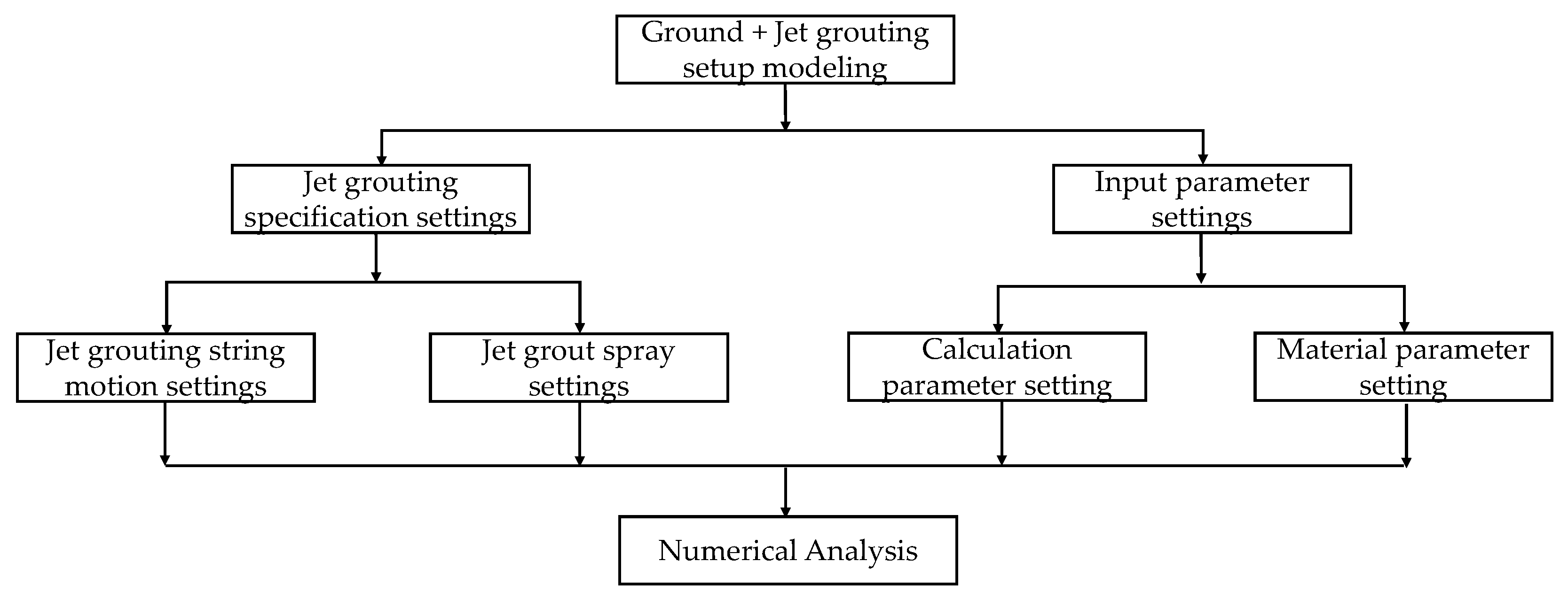
Figure 2.
Simulation model of jet grouting.
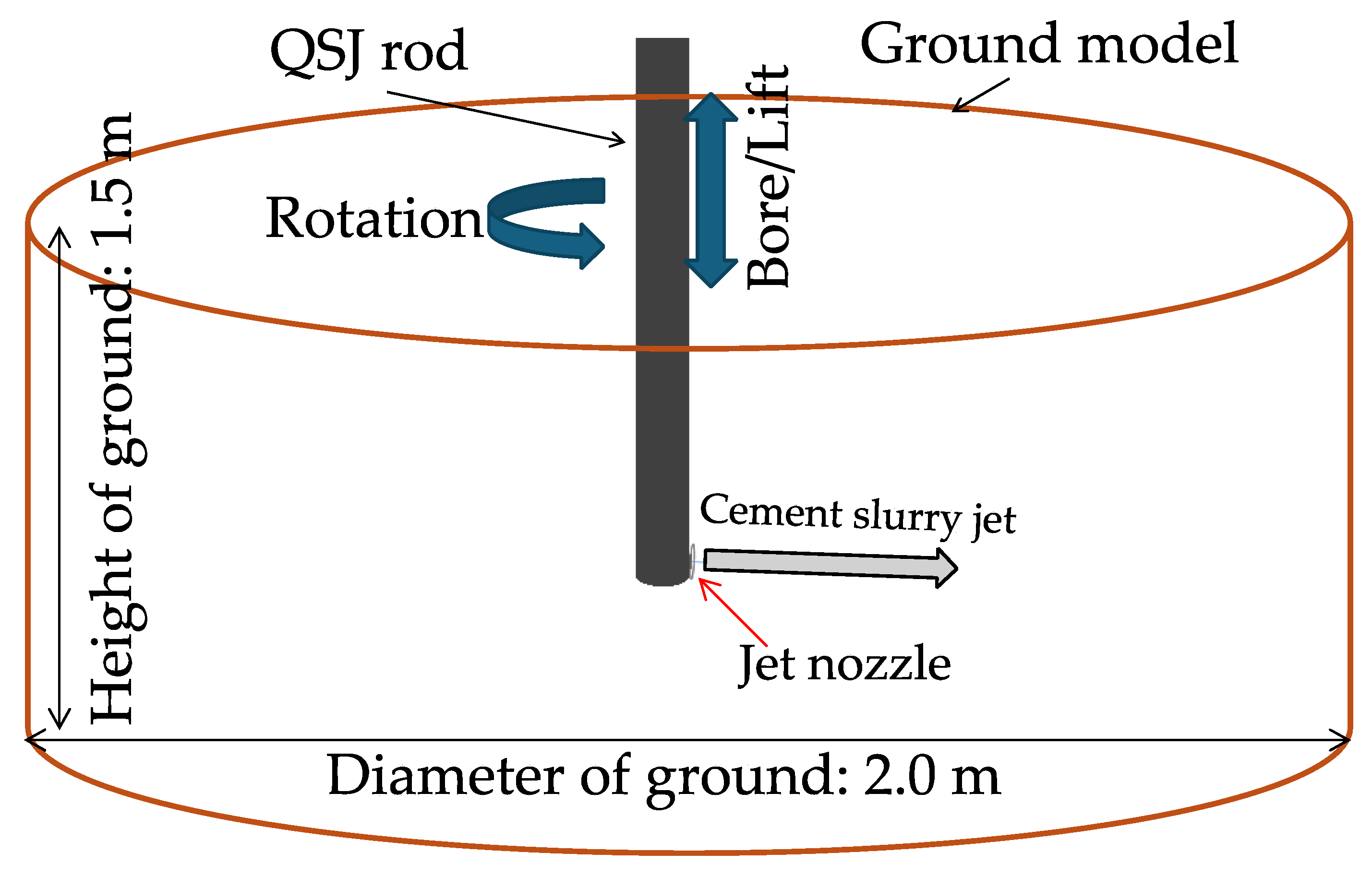
Figure 3.
Schematic comparison of fluid rheology models.
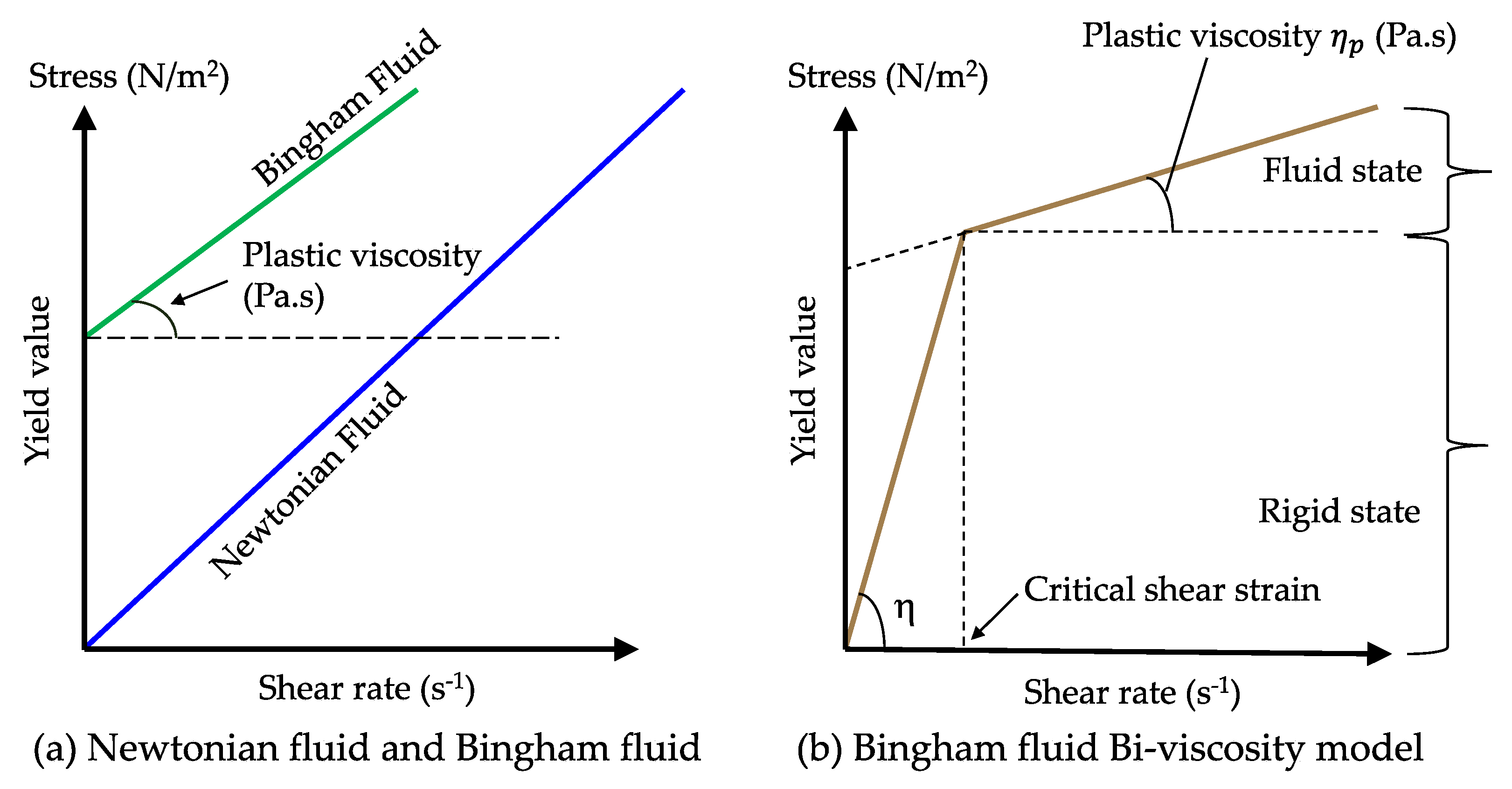
Figure 4.
B-type viscometer along with its spindles.
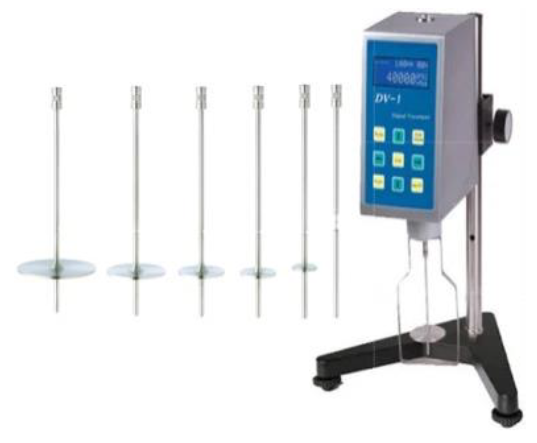
Figure 5.
Rheometer.
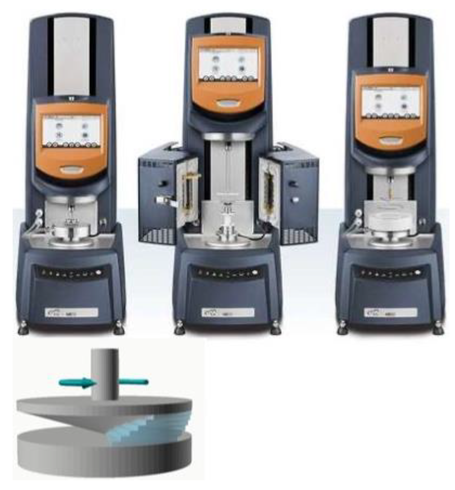
Figure 6.
Sensitivity analysis of yield parameter values for constant critical shear strain value.
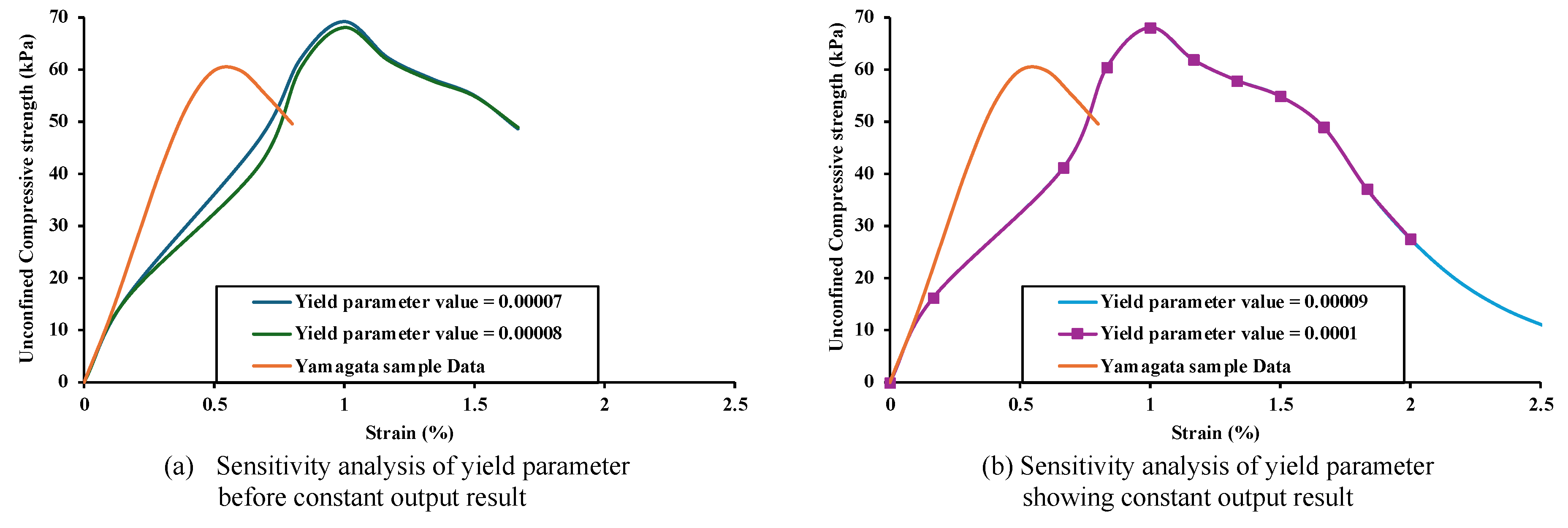
Figure 7.
Sensitivity analysis to determine a representative critical shear strain value.
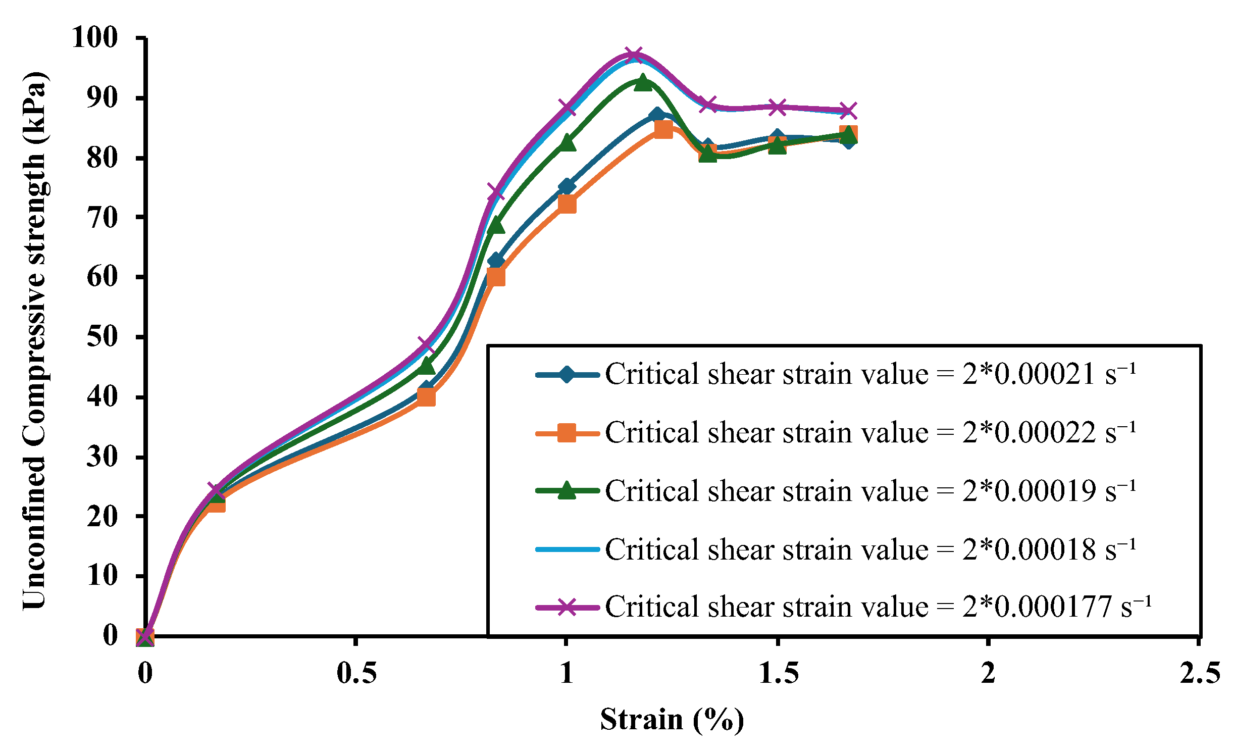
Figure 8.
Verification simulation for the recalculated critical shear strain value.
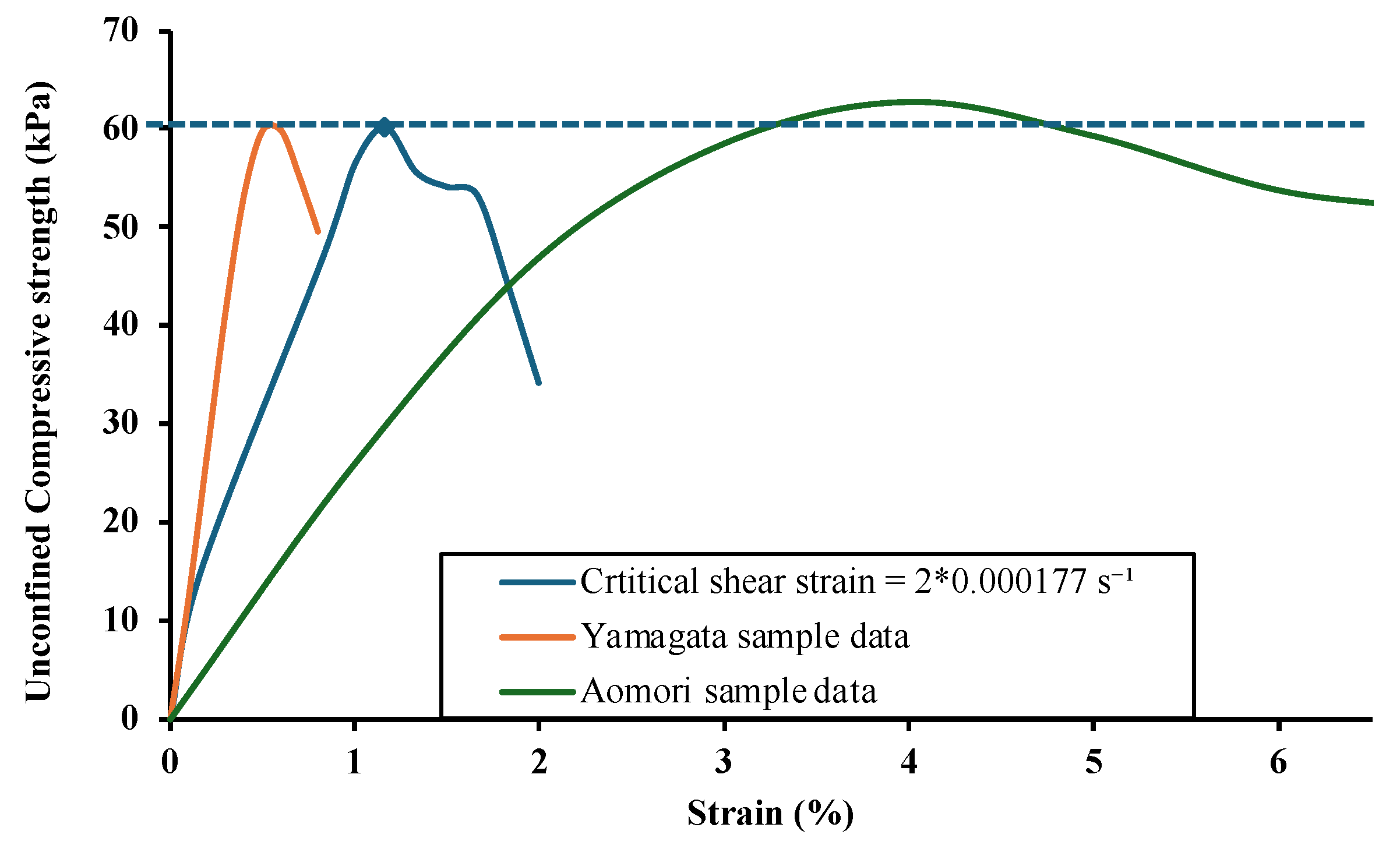
Figure 9.
Sensitivity analysis of the yield parameter to determine the representative value.
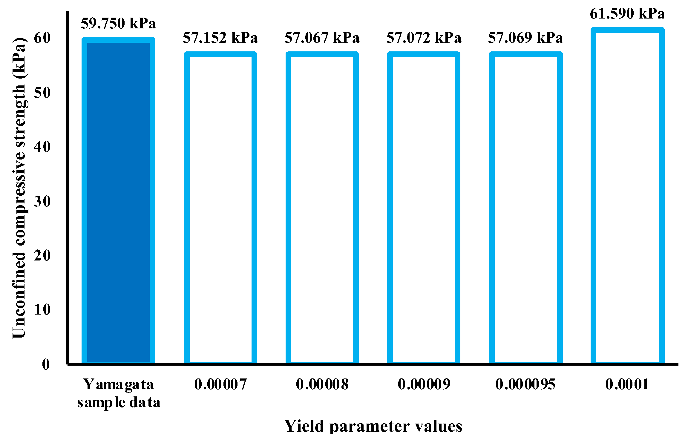
Figure 10.
Verification simulation for Sample 1 using representative values.
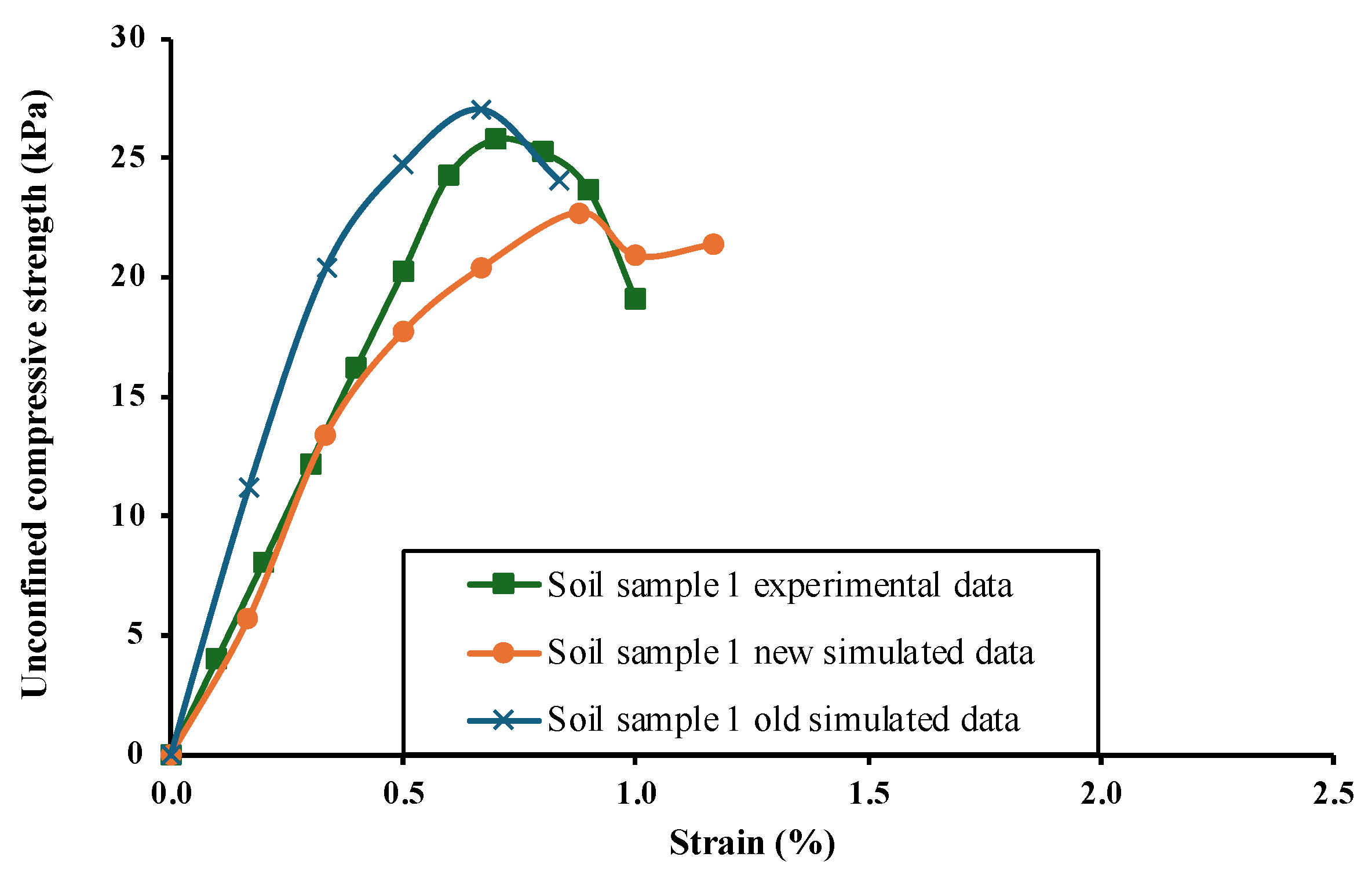
Figure 11.
Verification simulation for sample 2 using representative values.
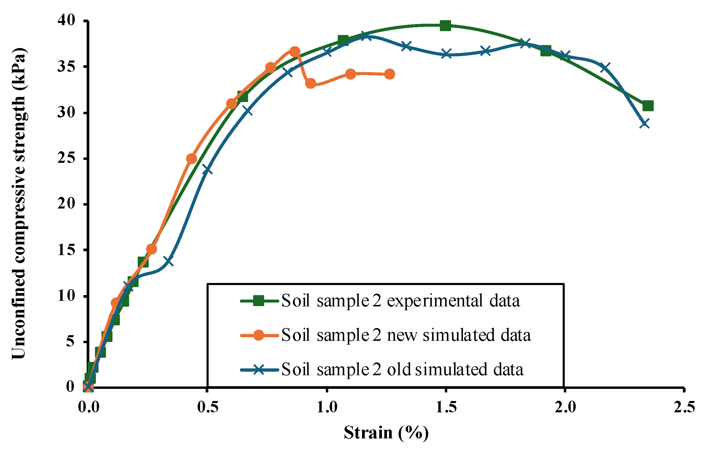
Figure 12.
Verification simulation for sample 3 using representative values.
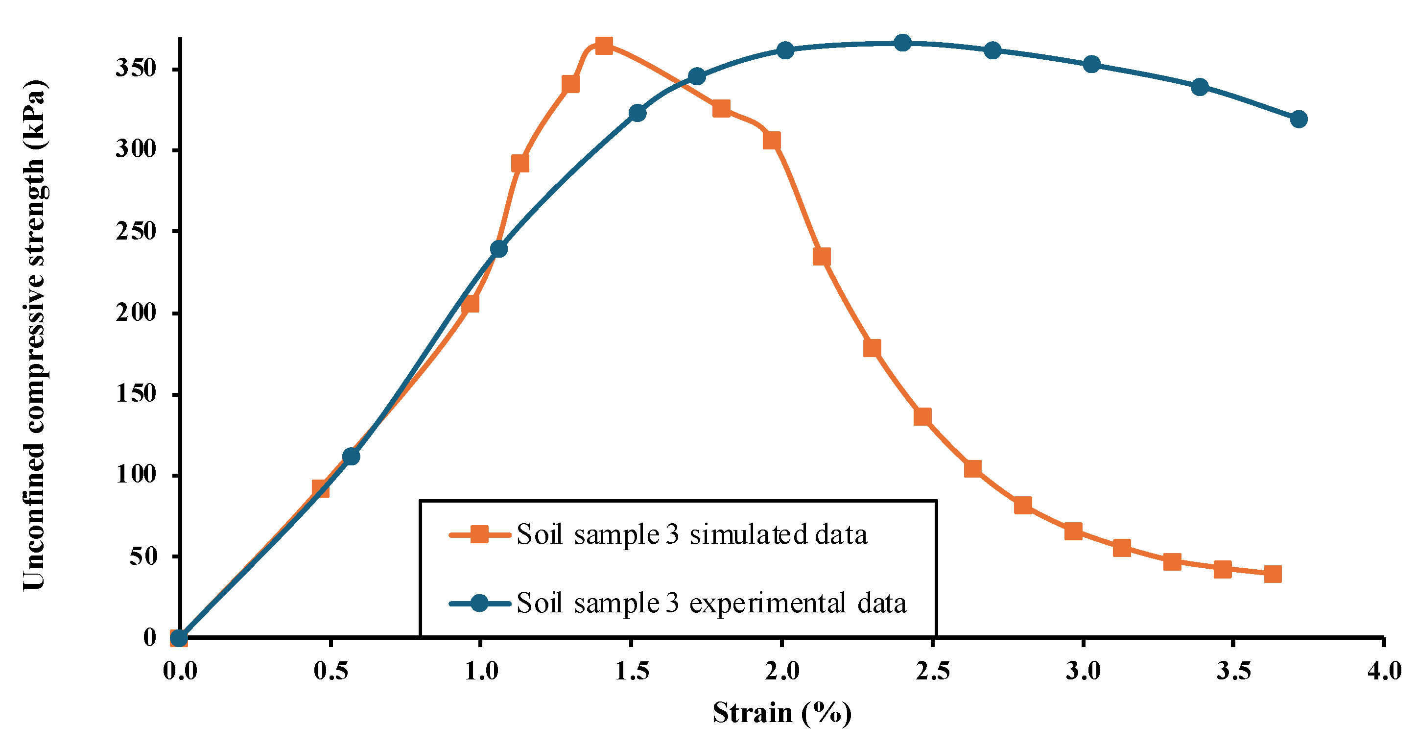
Figure 13.
Relationship between jet distance and jet flow pressure [2].
Figure 13.
Relationship between jet distance and jet flow pressure [2].
Figure 14.
Visualization of soil concrete formation from 360 direction.
Figure 15.
Top view to confirm maximum diameter.


Table 1.
Design specifications.
| Jet grouting specifications | Boring | Lifting |
| Grouting Material | Water | Cement slurry |
| Grouting period (s) | 20 | 58 |
| Boring depth without spray (m) | 0*1 | 0*1 |
| Grouting zone height (m) | 0.5 | 0.5 |
| Grout amount (L/min) | 80 | 90 |
| Grout jet pressure (MPa) | 9.4 | 18.0 |
| Grout jet velocity (m/s) | 137.5 | 155.0 |
| Boring speed of QSJ rod while improving soil (m/min) | 1.5 | - |
| Lifting speed of QSJ rod while improving soil (m/min) | - | 0.52 |
| QSJ rod rotation speed (rpm) | 20 | 20 |
| *1 Start and end of grouting position locating at the 0.5 m below the top surface | ||
Table 2.
Material parameters.
| Material | Density (kg/m3) | w/c | Yield value (Pa) |
Plastic viscosity (Pa.s) |
Yield parameter (-) |
Surface tension (N/m) |
Fluid model |
|---|---|---|---|---|---|---|---|
| Water | 1000 | - | - | - | - | 0.10 | Newtonian fluid |
| Cement slurry | 1500 | 1.0 | 10 | 0.28 | 0.0001 | 0.10 | Bingham fluid |
| Ground | 1600 | - | 30000 | 17000 | 0.0001 | 0.002 | Bingham fluid bi-viscosity model |
Table 3.
Computational and material parameter settings for sensitivity analysis of critical shear strain.
Table 3.
Computational and material parameter settings for sensitivity analysis of critical shear strain.
| Initial time interval (s) | Interparticle distance (mm) | Yield value (kPa) | Yield parameter |
Plastic viscosity (Pa.s) | Critical shear strain (s-1) | Output strength (kPa) | Strain (%) |
|---|---|---|---|---|---|---|---|
| 0.05 | 0.5 | 50,000 | 0.000100 | 23,810 | 2*0.00021 | 87.1 | 1.215 |
| 0.05 | 0.5 | 50,000 | 0.000100 | 22,730 | 2*0.00022 | 84.67 | 1.23 |
| 0.05 | 0.5 | 50,000 | 0.000100 | 26,315 | 2*0.00019 | 92.79 | 1.182 |
| 0.05 | 0.5 | 50,000 | 0.000100 | 27,780 | 2*0.00018 | 96.2 | 1.163 |
| 0.05 | 0.5 | 50,000 | 0.000100 | 28,250 | 2*0.000177 | 97.29 | 1.158 |
Table 4.
Comparison of material parameter values after using representative soil parameters.
| New simulation | Old simulation | |||
| Sample 1 | Sample 2 | Sample 1 | Sample 2 | |
| Yield value (kPa) | 12,900 | 19,743 | 12,900 | 19,743 |
| Plastic viscosity (Pa.s) | 7,300 | 11,200 | 10,000 | 13,162 |
| Yield parameter | 0.0001 | 0.0001 | 0.0001 | 0.00008 |
| Critical shear strain (s-1) | 2*0.000177 | 2*0.000177 | 2*0.000129 | 2*0.00012 |
Disclaimer/Publisher’s Note: The statements, opinions and data contained in all publications are solely those of the individual author(s) and contributor(s) and not of MDPI and/or the editor(s). MDPI and/or the editor(s) disclaim responsibility for any injury to people or property resulting from any ideas, methods, instructions or products referred to in the content. |
© 2024 by the authors. Licensee MDPI, Basel, Switzerland. This article is an open access article distributed under the terms and conditions of the Creative Commons Attribution (CC BY) license (https://creativecommons.org/licenses/by/4.0/).
Copyright: This open access article is published under a Creative Commons CC BY 4.0 license, which permit the free download, distribution, and reuse, provided that the author and preprint are cited in any reuse.


