
Submitted:
14 January 2025
Posted:
15 January 2025
You are already at the latest version
Abstract
This study examines the conversion of an overflow ball mill into a new energy-efficient discharge system via Discrete Element Method (DEM) and Smoothed Particle Hydro-dynamics (SPH) simulations. The research evaluates milling charge dynamics, empha-sizing the impact of liner geometry and operational variables such as charge filling and ball size. Our methodology integrates SPH to assess effects of the slurry on energy dissipation, power loss, breakage rates, and material transport. Our findings highlight significant operational inefficiencies in the overflow setup, notably extensive dead zones and excessive charge volume that hinder milling efficiency by limiting slurry in-teraction and reducing energy for comminution. Additionally, slurry pooling shifts the center of gravity, causing torque losses and direct material bypass to the discharge zone. Our simulations replicate these challenges and benchmark them against indus-trial-scale operations, identifying critical charge excesses that constrain throughput and elevate power consumption. The new discharge system decouples the filling charge from the evacuation mechanism, further than tackling common issues in the traditional grate discharge setups like backflow and carry-over. This approach substantially improves grinding efficiency, as demonstrated by enhanced breakage rates and diminished specific energy consumption. The results provide a robust framework for mill design and operational optimization, underscoring the value of integrated slurry behavior analysis in mill performance enhancement.
Keywords:
DEM-SPH coupling
; overflow ball mill
; grate discharge
; EEPL
; slurry pooling
1. Introduction
1.1. Ball Mill
In mineral processing, ball mills are responsible for reducing particle size of minerals, and critical for the successful liberation and recovery of valuable metals through processes such as flotation. As the mining industry contends with declining global ore grades and increasing mineral complexities and hardness, the efficiency of grinding operations has become central to the economic viability of the sector.
The operation of ball mills involves rotating a cylinder filled with grinding media at a speed that varies depending on the mill’s diameter. It is where the finer comminution of ores with diverse mineralogies takes place. Grate discharge mills, in particular, are designed to limit over-grinding and conserve energy by allowing only the finely ground product to pass through the grates. This selective retention and evacuation process significantly enhances the efficiency of the grinding process.
Traditionally, the industry has relied on overflow ball mills due to their simplicity and effectiveness across a variety of ore types. In an overflow mill, the material exits over the spillway, resulting in a very fine product size. However, with the evolving characteristics of mined ores, there is a growing need for more controlled milling operations to handle these changes effectively.
As an alternative, a new energy efficient pulp lifting system has been designed to offer a more selective grinding mechanism. Unlike overflow type, the proposed design utilizes a diaphragm at the discharge end featuring a grate system that retains larger particles and grinding media, allowing only sufficiently ground particles to exit the equipment. This setup not only prevents unnecessary regrinding particles but also enhances operational efficiency by improving the quality of the grind and reducing energy consumption. The innovation lies on incorporating deflectors that prevent the slurry from returning to the mill chamber and curved vanes that effectively flush out material. This is coupled with adjustments to operating parameters, specifically the selection of grinding media and its filling load in the mill, which are tailored based on the new breakage rates required under these updated conditions.
In this context, adopting more energy and cost-efficient milling technologies becomes essential, where even marginal improvements in mill design and operation can result in substantial economic and environmental benefits.
1.2. Simulation Tools
The efficiency of these operations and equipment hinges on understanding the behaviors of the fluid and granular solid particles during the grinding process, which are significantly impacted by the interaction dynamics within the mill.
Advanced simulation tools, such as Discrete Element Method (DEM) coupled with Computational Fluid Dynamics (CFD), are essential for accurately modeling these interactions. These tools allow for a comprehensive analysis of how changes in particle design—such as modifications to surface area, density, and shape—affect grinding. This level of detail is critical in ball mills, where the precise interactions between particles can significantly influence the efficiency of the mineral liberation process.
The necessity of these simulations is not for only understanding what happens inside the mill but also for optimizing operations and extending their applications to circuits processing increasingly complex and harder ores. The case study of application at an industrial scale presented here illustrates the practical benefits of implementing such advanced models.
By leveraging these simulation tools, engineers are equipped to design ball mills, mill linings, discharge systems, select the appropriate ball top-up, and set the right operating parameters. This approach not only improves the operational efficiency of ball mills but also contributes to the broader goals of enhancing the sustainability and cost-effectiveness of mining operations.
1.3. Meshless Lagrangian methods
Eulerian methods, commonly used in traditional CFD, involve discretizing the fluid domain into a fixed grid system where the fluid properties at each grid point are calculated over time. This approach provides a stable framework for analyzing fluid flow, especially in scenarios involving complex boundary interactions and steady-state flows. The primary advantage of Eulerian methods is their ability to handle problems where the geometry of the domain does not change significantly over time, making these methods highly effective for studying flow around solid objects or through channels [1].
However, Eulerian methods face significant challenges in capturing large deformations within the fluid, such as those occurring in free-surface flows or highly dynamic interfaces. These methods also struggle with the computational cost associated with refining the mesh to capture finer details, which becomes necessary in the presence of complex fluid behaviors.
In contrast, Lagrangian methods treat the fluid domain by tracking individual fluid particles as they move through space and time. This approach naturally accommodates large deformations and dynamic changes in the fluid’s topology, making it particularly suited for simulations involving complex interactions between fluids and moving boundaries. In the Lagrangian framework, the fluid is not constrained by a fixed spatial grid; instead, fluid particles carry their properties and interact based on their positions, which continuously update over time.
The material derivative formula integral to Lagrangian methods:
directly captures the advection of fluid particles, facilitating a more natural and detailed simulation of fluid dynamics [2]. This method’s adaptability to changing fluid geometries offers a significant advantage in simulations where fluid structure interactions play a critical role.
Despite their flexibility, Lagrangian methods, particularly those implemented in meshless frameworks like Smoothed Particle Hydrodynamics (SPH), encounter difficulties with accuracy at boundaries and in regions of sparse particle distribution. These issues often result in numerical instabilities or require complex corrections to ensure the fidelity of the simulation. The misinterpretation of empty computational spaces as valid fluid areas is a notable challenge, often requiring enhancements in kernel functions or more sophisticated interpolation schemes to mitigate errors [03, 04–07].
The SPH method has evolved significantly since its inception to address these challenges, incorporating improvements in particle weighting and distribution techniques to enhance simulation accuracy and stability. Recent advancements have also explored coupling SPH with traditional grid-based methods to leverage the strengths of both Eulerian and Lagrangian approaches, providing a hybrid solution that maximizes accuracy while maintaining computational efficiency [8].
Considering the inherent limitations of Eulerian methods, particularly in handling dynamic interactions and complex boundary conditions within our fluid-solid system, we have chosen to adopt the Meshless Lagrangian method for our simulations. The Smoothed Particle Hydrodynamics (SPH) technology, a subset of the Lagrangian approach, offers the flexibility and precision necessary to effectively model and predict the outcomes of modifications made to the discharge system in ball mills. The decision to utilize SPH was informed by its capability to accurately track and simulate the movements and interactions of individual particles within the fluid medium of the ball mill. This approach proved invaluable, as it allowed us to achieve results that closely align with the empirical data observed at an industrial level. The fidelity of SPH simulations to real-world phenomena, therefore, not only validates our methodological choice but also enhances our confidence in the predictive power of our computational models, ensuring that our design improvements are both scientifically grounded and practically viable.
1.4. Mass-Momentum Coupling of the Fluid Phase
The Navier-Stokes equations govern the evolution of a fluid, expressed in a Lagrangian framework as follows:
where is the fluid density, the fluid velocity, the pressure, the kinematic viscosity, and the body force. These equations are linked by a state equation that dictates how properties such as density and pressure interrelate, especially significant when considering fluid motion’s evolution. In the context of a compressed liquid, pressure directly relates to density.
In scenarios with negligible density variations, the system’s density remains relatively constant. To address this in fluid simulations, particularly when the fluid is nearly incompressible, a constraint is applied to ensure the flow is divergence-free:
To implement this, meshless methods like the moving semi-implicit (MPS) and smoothed particle hydrodynamics (SPH) often use projection techniques to isolate and retain only the divergence-free velocity component. This truncation is essential for solving the pressure Poisson equation (PPE), expressed as:
where represents a source term derived from the mass density rate of change. Handling this linear system effectively is critical, especially in large-scale simulations where the incompressibility assumption must hold under variable flow conditions.
Furthermore, under extreme conditions where fluid velocities significantly exceed the sound speed, as in underwater explosions or very fast flows, it is possible to adopt a pressure-density relationship that adjusts dynamically:
with as the reference pressure, the reference density, and the adiabatic index. This formulation facilitates the simulation of incompressible flows by effectively coupling the fluid’s density and pressure [9].
Choosing a numerical sound speed much lower than the actual physical sound speed, yet considerably higher than the maximum fluid velocity, allows simulations to approximate incompressible fluid behavior more effectively, a method crucial for achieving stability and accuracy in fluid dynamics simulations.
1.5. Numerical Methods for Fluid-Particle Coupling
Coupling between a fluid and a solid phase is essential for accurately predicting the interactions within multiphase systems. One-way coupling focuses merely on the forces exerted by the fluid phase onto the solid phase. In contrast, two-way coupling enhances the model by redistributing these forces back onto the fluid phase, allowing an exchange of force information between solvers. This method only involves the transfer of information and necessitates independent frameworks for each solver to manage this data exchange, as depicted in Figure 1, which outlines the general structure of the coupling process.
Various strategies are employed to determine the coupling force, with the choice of strategy influencing the implementation’s complexity and accuracy. These can be broadly classified into two categories: direct-resolved and under-resolved approaches. Direct-resolved strategies require physically resolving the fluid flow around individual solid particles, thereby directly capturing the interactions between the fluid and solid phases. This method facilitates a reduction in the need for additional simplifications or empirical models and ensures that both the fluid and solid systems can be treated as independent entities, thereby streamlining the simulation process.
In contrast, under-resolved strategies involve determining a back-coupling force based on experimental correlations or analytical formulations, automatically managing boundary conditions during this process. The efficacy of direct-resolved versus under-resolved strategies is heavily dependent on the specific requirements of the simulation.
A notable example of a direct-resolved approach is the no-slip boundary conditions scheme, where the fluid is not allowed to penetrate the solid particle surface, a method meticulously detailed by Potapov et al. [10]. This ensures accurate adherence to the physical properties expected in such interactions, providing a high-fidelity model of fluid-solid dynamics.
Conversely, under-resolved methods offer a computational advantage by integrating a spatially averaged version of the fluid’s governing equations, which simplifies the computational load and allows for the inclusion of larger particle systems, including non-spherical shapes. This approach, as described by Potapov et al. [10], emphasizes efficiency and scalability, essential for large-scale simulations.
Figure 1 presents a flow diagram of the coupling scheme between Discrete Element Method (DEM) and Meshless Methods (M.L.M.), illustrating the sequence from initial condition settings through to the integration of interaction forces and the final time step of the simulation. This diagram highlights the procedural steps and decision points critical to the integration process, showing how each part of the system interacts and contributes to the overall simulation workflow.
Despite the flexibility offered by direct-resolved strategies, the high computational cost often makes under-resolved strategies more appealing for extensive or complex simulations. Future studies may focus on optimizing these methods, potentially integrating the strengths of both to enhance efficiency and applicability across various simulation scales and conditions.
2. Materials and Methods
2.1. SPH Formulation
This section presents the key formulas and numerical techniques implemented in DualSPHysics [11] based on the SPH method. The Navier-Stokes (N-S) equations describing fluid behaviour are resolved using weakly compressible SPH (WCSPH) formulas. The continuity equation and momentum equation implemented in DualSPHysics are provided below,
where i is the target particle and j is the neighbor particle of particle i. The free parameter δ is set as 0.1 in our study, and g is the gravity acceleration. corresponds to a density diffusion term that stabilizes the density field when experiencing high-frequency oscillations.
Where . The superscripts “T” and “H” indicate the total and hydrostatic components, respectively. The artificial viscosity term is presented as follows:
To circumvent the need to solve the Poisson pressure equation, a weakly compressible model uses the following equation of state:
where is the reference density and is set to 7 in this study. The compressibility of the fluid is defined by the numerical speed of sound, , which is determined as follows:
Here, is the maximum velocity and is the undisturbed depth of the fluid. This formula aims to limit relative density fluctuations to less than 1%. In addition, the Quintic Wendland kernel [30] has been chosen for this work, and the smoothing length is set to 1.2 times the SPH particle spacing (). This configuration results in a kernel interaction distance of 2.4 .
In this study, denotes the maximum velocity, and indicates the undisturbed fluid depth. The objective of this formula is to limit relative density fluctuations to less than 1%. Additionally, the Quintic Wendland kernel [30] has been selected, setting the smoothing length to 1.2 times the SPH particle spacing (). This configuration establishes a kernel interaction distance of 2.4 .
The Modified Dynamic Boundary Condition (MDBC) is utilized here to ensure stability in the pressure field near the boundary, aiming to address interaction discrepancies between dynamic boundaries and fluid particles [12]. In managing boundary particle arrangements, MDBC adheres to similar procedures as the conventional DBC. Nonetheless, boundary particles are often layered multiple times, with the boundary interface strategically positioned at half the distance of the innermost boundary particles ().
Using the MDBC approach, a ghost node is established for each boundary particle within the fluid domain. Normal vectors, emanating from the boundary particles towards the boundary interface, dictate the direction within the fluid domain. This method enables the derived normal vector to project onto the ghost particle. Fluid properties are subsequently accurately approximated using corrected SPH at the ghost node and then reflected onto the boundary particles. The DualSPHysics framework efficiently maps boundary ghost particles of diverse shapes.
Comprehensive details on the implementation can be found in [13].
In DualSPHysics, accurate integration of particle properties such as position, velocity, density, and pressure over time is achieved via the utilization of a Symplectic algorithm [14]. Further details about this algorithm within DualSPHysics are provided in [15]. To ensure numerical stability, DualSPHysics employs the CFL (Courant-Friedrichs-Lewy) condition and implements a variable time step () [16]. Adherence to the CFL condition is crucial for maintaining both accuracy and stability in simulations.
where is the force per unit mass exerted by the fluid particle on the boundary particle . Further, we can obtain the and of the rigid body from the SPH particles as shown below,
where is the position of particle , is the center of mass of the rigid body , and is the fluid force on boundary particle according to Eq. (12).
2.2. DEM Theory
Spherical particles are commonly used in simulations using the DEM due to their fast and straightforward nature, which simplifies contact detection and force calculations [17]. However, this simplification often fails to capture the dynamic behaviour of real particle materials adequately, which is considered unacceptable [18]. To address this limitation, researchers have developed various particle shape approximations in DEM simulations. These include ellipsoids [19], hyperquadric [20], multi-sphere [21], polyhedron [22] and other shapes. By incorporating these alternative shapes, simulations can better represent the intricate dynamics exhibited by real particle materials, enhancing the accuracy of the models.
Modelling irregularly shaped particles in fluid-structure coupling frameworks remains a challenge, particularly when it comes to their interaction boundaries with fluids. In this work, polyhedral particles are employed to consider the influence of shape factors on the dynamic behaviour of particles via the Blaze-DEM solver. Polyhedral geometry is read as an STL (Standard Triangle List) mesh as depicted in Figure 2a. Triangles connected with similar orientation are then merged as depicted in Figure 2b to create feature edges and vertex. Finally, as shown in Figure 2c, the unique polygon faces are defined including the center point and the normal direction (Only one face is shown, and the others will be treated as well). The above treatment allows the polyhedron to be represented as a collection of planar faces and feature edges, which are used along with vertices for detailed descriptions of contact calculations between polyhedrons. For a more detailed understanding, please refer to [23].
Contact detection is the most time-consuming part of DEM simulation, accounting for around 90% of the overall simulation time. To address this issue, the coupling model proposed in this work employs a three-stage process to identify potential DEM particle contact pairs, including the “broad phase,” the “intermediate phase,” and the “narrow phase” (as shown in Figure 3). In the “broad phase” (Figure 3a), a grid-based spatial partition hashing strategy is utilized to list the neighbours of potential particles. For polyhedral particles, the “broad phase” is followed by a more accurate “intermediate phase” (Figure 3b) that uses some boundary primitives to detect contact, which is more efficient than performing a full contact check. This is followed by a “narrow phase” (Figure 3c) to establish contact pairs and ultimately contact measures to calculate force directions and magnitudes. The details of the contact detection algorithms can be found in [12,16,17].
In DEM simulations, calculating the contact force between solid particles is crucial for predicting their motion response. This study introduces a new contact law [24] based on overlap volume to the SPH-DEM coupling model for polyhedral collision resolution. This modified approach significantly improves the robustness of interactions between polyhedral particles. It includes a Kelvin-Voigt linear viscoelastic spring dashpot for rigid particles, which generates an elastic force that stores energy and an energy-dissipative Coulomb force. These advancements enhance the accuracy and reliability of DEM simulations involving irregularly shaped particles, particularly in fluid-structure interactions. The normal force Fn between contacting olyhedral is given by a spring dashpot model [23] as:
where is the volumetric spring stiffness (), is the overlap volume, is the damping coefficient (), is the relative velocity, represents the normal at contact. and can be written as,
where represents the effective mass of the DEM particles, ϵ represents the restitution coefficient and is the contact time, that is determined by properties of the material and is selected such that physical quantities of interest (such as energy) are conserved during integration for the typical range of velocities observed in the simulations [25,26]. For all simulations in this study, we employ a contact time equivalent to at least 10-DEM time steps and the DEM time step is set to 1 s. The overlap volume and contact normal are resolved exactly for two polyhedral shaped particles in contact as depicted in Figure 4. By resolving the contact points between two intersecting polyhedral particles (P1, P2 in Figure 4a), the convex hull is constructed to calculate the contact volume (Figure 4b). The corresponding contact normal and particle forces are analyzed for each particle depicted in Figure 4. Detailed information can be found in [18,27].
The tangential force is computed as the sum of the tangential spring force and a tangential viscous force:
where is the volumetric spring stiffness, is overlap volume, is the damping coefficient, is the tangential spring stiffness (), r represents the relative tangential velocity, is the time step, is the tangential spring displacement from its equilibrium position. represents the tangential damping coefficient. More details can be found in [23,27].
Finally, the contact force and torque acting on this DEM particle is obtained:
where is position of DEM particle contact point, is the mass center of current DEM particle.
The translational motion and rotational motion of the DEM particle k is solved with the Newton’s second law:
where and represent the mass and moment of inertia matrix of DEM particle . and are the translational and angular velocities, respectively. and indicate the net force and torque on the DEM particle , with the superscript and representing the force or torque obtained from the solid and fluid phases, respectively.
2.3. Coupling Strategy
Figure 5 shows how the liquid and solid phases are treated in the proposed coupling algorithm. In the SPH solver, the fluid is discretized into particles for calculation, where the polyhedron is discretized into a series of particles to obtain the fluid force. DualSPHysics calculates the fluid forces of the SPH-SPH interacting particles to update the fluid domain according to the fluid conservation equation. At the same time, the fluid force of SPH particles on rigid particles is calculated. In DEM solvers, polyhedral are described as rigid bodies (with material properties) with points, lines, surfaces, and other characteristics, and with interaction that follow the law of contact. The consistency of all polyhedron information is crucial for achieving accurate two-way coupling between the two solvers, including spatial information and its own properties. Blaze-DEM calculates the contact force of the multi-body system while considering the fluid force as the external force received from the SPH solver. The particle motion information is then acquired and transmitted to DualSPHysics for rigid body updating.
Figure 6 illustrates a flow chart depicting the fluid-solid coupling simulation process. This simulation utilizes three modules: the SPH module, the DEM module, and the coupling module. In this process, the SPH module acts as the main loop, controlling the overall program. It communicates the fluid force and the current SPH time step to the DEM solver via the coupling module. The DEM solver then takes these inputs and iterates through its inner loop multiple times until the termination condition is met (). Upon meeting the termination condition, the particle motion information is transmitted back to the coupling module for updating on the SPH side. Subsequently, the SPH solver incorporates this updated particle motion information and fluid domain, preparing them for the next cycle. The detailed numerical implementation is as follows:
- Calculate the SPH time step ;
- Update the neighbor list for SPH particles;
- Solve the SPH governing equations Eq. (6) and Eq. (7) for particles interaction involving fluid-rigid object and fluid-fluid;
- Obtain the fluid force and torque by Eq. (8) and Eq. (9) applied to the rigid body, and transmit to the DEM module together with the SPH time step;
- DEM particles search for neighbor particles and calculate contact forces and torque by Eq. (14) and Eq. (15);
- Apply and as external forces to get calculate acceleration and angular acceleration of DEM particles via Eq. (16) and Eq. (17);
- Update velocity, angular velocity, and position of DEM particles;
- Determine whether the DEM loop is complete: If not, continue from step 5 until the end; If so, the DEM particle information is sent to the coupling module;
- Update the SPH particles and rigid body information in SPH module, and the system is ready to calculate for the next SPH time step (If any).
The Smoothed Particle Hydrodynamics (SPH) is applied in this research to model slurry transport in ball mills, replicating real-world conditions to enhance understanding of rheology in full, evacuation, power spectra and other phenomena. Recent advancements in slurry transport and grinding dynamics modeling have further refined this approach. Cleary et al. (2006) introduced a coupled DEM-SPH framework for predicting slurry transport in SAG mills, which became a cornerstone for subsequent studies. Cleary and Morrison (2012) extended this work by developing 3D models of slurry flow and discharge behavior, capturing the intricate dynamics of grinding chambers. Further, Cleary et al. (2020) employed DEM-SPH to investigate interactions between grinding media, coarse rocks, and slurry, elucidating slurry grinding mechanisms. Cleary, Cummins, and Sinnott (2020) advanced these methods to focus on mill wear and slurry-phase grinding effects. Collectively, these studies underscore the transformative potential of particle-based simulations in optimizing mill operations and improving efficiency [35,36,37,38].
2.4. Industrial-Scale Implementation
To thoroughly examine the internal dynamics of the ball mill, the Discrete Element Method combined with Smoothed Particle Hydrodynamics (DEM-SPH) approach was utilized. To substantiate the conclusions drawn from this method, a detailed industrial-scale conversion was conducted, involving the complete transformation of an overflow ball mill into a grate discharge configuration. This comprehensive modification not only involved changing the discharge system but also included a complete redesign of the mill liners. Specifically, the face angle of the lifters was adjusted to enhance the charge motion, optimizing energy utilization towards size reduction.
The industrial-scale implementation selected two distinct circuits, BM-5 and BM-6, both designed similarly. BM-5 was equipped with the traditional overflow discharge, while BM-6 incorporated a new discharge system featuring an advanced pulp lifting system. Both mills, although running in parallel configurations, were fed with the same material—ore that was blended and then split to ensure uniformity across both systems. This setup was crucial for a direct comparison of the two systems’ efficiency. Key performance indicators such as the particle size distribution (PSD), throughput (tph), and power consumption were measured and compared to evaluate the impact of the different discharge systems under identical feed conditions. This parallel approach not only facilitated an accurate assessment of the enhancements but also highlighted the potential benefits of the new discharge system in terms of operational efficiency and material handling.
The following procedural steps were undertaken using JKSimMet software with the provided data set:
- Mass Balancing: This step ensured the integrity and accuracy of material flow data by verifying that the total mass entering the system matched the total mass exiting it, accounting for feed, product, and recirculating loads. Accurate mass balancing not only validated the dataset but also provided a solid foundation for subsequent model adjustments and simulations. This process identifies and rectifies any inconsistencies or errors in the data, ensuring that the analysis reflected true operating conditions.
- Model Fitting (Model Preparation for an Existing Overflow Ball Mill): The model was calibrated to accurately replicate the operation of the existing overflow ball mill configuration. Parameters such as grindability, size distribution, and power draw were adjusted to align with real-world performance. This step ensured that the baseline model provided a reliable reference point for evaluating the impact of the proposed modifications. The calibrated model acted as a benchmark, allowing direct comparison between the current and modified setups while minimizing uncertainties in performance predictions.
- Model Simulations (Grate Discharge): Simulating the modified grate discharge setup to evaluate performance changes and optimize the mill operations post-modifications.
3. Results
3.1. Baseline Scenario: Overflow Configuration
The base scenario describes the operational parameters of the primary ball mill, tagged as BM-5 configured with an overflow discharge arrangement. This mill has an internal diameter of 4.41 meters, an internal length of 7.8 meters, operates at 74% of critical speed with Bond Work Index (BWI) of 15.5 kWh/t. It carries a ball load of 29% with ball top sizes of 75 and 60 mm. The accompanying hydro-cyclone classification system consists of two cyclones, each with a diameter of 0.50 meters, inlet diameter of 0.20 meters, vortex finder diameter of 0.19 meters, spigot diameter of 0.13 meters, cylinder length of 0.47 meters, and operates at a cone angle of 20 degrees and a pressure of 90 kPa. The PSD of the mill’s discharge and the overflow from the hydrocyclone, is detailed in the Figure 7.
For the circuit under discussion, which produces the specified particle size distribution, the throughput (tph) and power draw are presented in Figure 8. This data serves as a reference point and it will be used as a baseline for comparison with the results of the proposed configuration, which includes modifications to both the discharge system and operating conditions
3.1.1. Validation of the Mathematical Model and Numerical Methods
To validate the DEM-SPH model, we employed the baseline scenario mirroring the equipment at referred industrial setting. Moreover, the model was calibrated and tested against standard known cases. The validation procedure is fundamental to ensure that the numerical method accurately replicates the physical behaviors observed at the industrial scale.
For the DEM simulations, critical coefficients such as the restitution coefficient (ε), friction coefficient (μ), and the stiffness coefficient (k) were finely adjusted. These parameters define the collision dynamics and energy dissipation within the mill. Specifically, the restitution coefficient was set to approximate the loss of kinetic energy upon impact, while the friction and stiffness coefficients influenced the tangential force and the normal force response during particle contacts.
For the SPH simulations, several key parameters were configured to enhance the fidelity of fluid dynamics modeling. These include the smoothing length, which defines the interaction radius of particles, and the particle mass, crucial for accurate momentum exchanges. Fluid properties such as viscosity and the stiffness coefficient were adjusted to reflect real fluid behavior on both laminar and turbulent flows. The equation of state was applied to relate pressure and density, vital for modeling compressibility. Time step settings adhered to the Courant-Friedrichs-Lewy condition to balance simulation accuracy and computational feasibility. Finally, appropriate boundary conditions and Kernel functions were selected to ensure the simulated environment closely mirrored the physical conditions of the mill, aligning with the boundary constraints set in the DEM simulations.
Boundary conditions were defined to replicate the physical system constraints, including fixed walls and periodic boundaries where applicable. This setup ensured that the simulation space faithfully represented the mill’s operational environment.
Comparative analyses between the simulated results and the data extracted from the Distributed Control System (DCS) of the plant were conducted. The software predictions closely aligned with the recorded industrial data, confirming the reliability of the DEM-SPH approach under standardized conditions with a marginal difference of around 5%. This validation is shown in Figure 9, which illustrates the average power draw of the mill from DCS data, effectively showcasing the mill’s performance and the simulation’s precision in replicating these operational characteristics.
3.2. Trial Results
The trial undertaken involved modifications to the discharge system of the ball mill, transitioning to a non-conventional grate discharge arrangement. This novel system features a series of deflectors designed to prevent backflow, paired with crafted vanes that optimize slurry evacuation. Additionally, modifications were made to the liners profile to enhance the charge motion and fit to the new impact energy spectrum.
A significant change was made to the operating parameters, notably a reduction in the filling charge. The trial configuration saw the filling charge decreased by 50%, resulting in a new charge level of just 14% of the mill’s total effective volume. The top up balls size was also reduced from 75 and 60 mm to 50 mm. These adjustments were aimed at improving the breakage rates and overall milling efficiency.
The outcomes of these changes are detailed in Figure 10 and Figure 11. These figures provide a comparative analysis between the baseline setup and the trial configuration, highlighting the efficacy of the alterations in sustaining the particle size distribution under the new operating conditions, which involve a substantially reduced grinding media charge.
To guarantee accuracy and consistency in the data collected, both the grate discharge and overflow mills were sampled simultaneously using the same standardized protocols. A total of 10 samples were taken from each stream, allowing for a comprehensive analysis of the conditions across both discharge types. The sampling intervals were set to capture both transient variations and steady-state conditions, ensuring that the results are representative of typical operational behaviors. The samples were taken at 30-minute intervals, and the results, detailing the P80 of each stream for each sample, are presented in Table 1.
3.3. Energy Spectra Analysis
When the mill is in operation, impact energy between particle-particle and particle-surfaces (liners) contributes to the liberation of the fine powder. The amount of fines produced depends on the intensity and the frequency of the impact energy. Generally, particle-particle energy is smaller in magnitude than particle-wall impact energy as the bulk of the particles is closely packed, which limits the relative velocity among particles itself. Particle-wall impact tends to have higher impact energies caused by the cataracting particles which fall onto the toe region with higher velocity than any other portion of the mill.
For each material ground in a mill, there is a critical impact energy level that depends on the particle size and material characteristics. Capece et al. [31] identified that the relevant impact energy threshold specific to particle size is 2.64 x 10^-5 Joules, derived from a size-independent baseline. Consequently, in our analysis, we disregarded any impacts with energy below 2.5 x 10^-5 Joules as they do not contribute effectively to the grinding process.
The energy required to drive the mill varies depending on the ore type, properties of grinding media and operating conditions such as mill speed and fill volume, which means that input power is system dependent. Mill input power was calculated based on the torque generated by those particles which were colliding with the mill drum. For each time step, individual torques were summed from the contributing particles to obtain the instantaneous toque on the mill. Those particles which are not in contact (free flight) do not contribute to torque until they meet the mill drum. Instantaneous power consumption is the product of the total toque with angular mill speed (in rad/s), and it has an impulsive nature. Here, the average power was calculated and compared with the industrial-scale implementation as shown in the Figure 9.
Figure 12 illustrates a compelling finding in the comparative analysis of energy distribution between the two ball mill configurations: the overflow (SlurryOF) and grate discharge (SlurryGD). Notably, despite the grate discharge configuration operating with 50% fewer balls than the overflow configuration, the number of useful total impact energy events remains remarkably similar, leading to a more effective transfer of energy per event, i.e. collision among the several elements inside the mill.
In addition to the consistent impact energy events, the operational efficiencies between the overflow and grate discharge configurations exhibit significant disparities. The power draw in the proposed setup was substantially reduced, dropping from 2214.5 kW in the overflow configuration to 1490 kW. This reduction in power was accompanied by an enhanced throughput of about 24.22%, where the mill with new design processed 159 tph, a noticeable improvement over the 128 tph processed by the overflow mill as illustrated in Figure 13. Consequently, these adjustments resulted in a reduction in specific energy consumption from 17.34 kWh/t to 9.38 kWh/t in the new discharge configuration, marking a decrease of approximately 45.93% in energy usage. These notable enhancements highlight the advantages of the new discharge system, particularly its superior energy efficiency and increased production capacity. These benefits yield a revenue increase while simultaneously reducing operational costs.
3.2. Slurry Pooling
In exploring the dynamics of mill operation, particularly concerning slurry pooling and its implications on power consumption, the work of Latchireddi and Morrell provides profound insights. Latchireddi and Morrell’s research delineates how slurry pooling in tumbling mills can substantially reduce power draw, a phenomenon that becomes particularly evident in ball mills operating under overflow conditions, where a slurry pool is always inherently present [28,29,32,33]. This reduction in power is contrasted with grate discharge mills, which do not typically operate with a slurry pool and, hence, tend to draw more power.
Morrell’s models, suggest that power draw in overflow mills is consistently lower than that in grate discharge mills due to the slurry pooling effect. This is quantifiable by modifying the mill’s discharge mechanism in predictive models from grate to overflow, which visibly decreases the power draw.
To further enhance our understanding, we utilized the robust capabilities of Discrete Element Method coupled with Smoothed Particle Hydrodynamics (DEM-SPH) properly calibrated to capture the nuanced effects of slurry pooling, particularly within overflow ball mill configurations. The simulations reveal that maintaining an ideal ore-ball ratio does not make possible the slurry evacuation, leading to excessive slurry within the mill on its standard running condition. This excess, in turn, hampers the ore-ball interaction, dissipates energy, and induces torque loss, culminating in diminished power draw and operational inefficiency. These findings not only corroborate the theoretical discussions presented earlier but also provide a visual framework to appreciate the operational challenges and potential adjustments needed for enhanced mill performance. Figure 14, Figure 15, Figure 16, Figure 17 and Figure 18, derived from our DEM-SPH simulations, vividly demonstrate these effects, offering a visual complement to the analytical discourse.
Figure 14 through 16 illustrate the impact of varying slurry levels on the operational dynamics of a ball mill, with changes in both the slurry-ball and ore-ball ratios.
Figure 14 presents a baseline scenario with both the slurry and the total charge (balls plus ore) at 34% of the mill’s volume ( and , respectively). In this configuration, the mass of balls totals 28.70 tons within a volume of 3.69 m³. The slurry fills the void spaces, totaling 2.70 m³, approximating the simulation value of 2.90 m³. The slurry-to-ball volume ratio stands at approximately 15.1%-84.9%, with the ore-to-ball volume ratio at 11.7%-88.3%.
Figure 15 depicts increase in slurry level while maintaining a constant ball volume at 34% (), resulting in the total charge level escalating to 44.9% (). In this scenario, the ball mass and volume are consistent with the baseline configuration, but the slurry volume is elevated to 4.75 m³. This change modifies the slurry-to-ball ratio to 23.8%-76.2% and the ore-to-ball ratio to 17.9%-82.1%. The intention behind this adjustment was to determine whether the increased slurry level would suffice to reach the mill’s outlet zone, which it did not achieve. However, we observed a notable reduction in power consumption, with a 28% decrease, highlighting the impact of slurry levels on mill efficiency.
Figure 16 further elevates the slurry level to a total charge of 55% () while maintaining the ball volume at 34% (). The ball parameters remain the same as in Figure 14 and 16, but the slurry volume increases to 6.65 m³, adjusting the slurry-to-ball ratio to 30%-70% and the ore-to-ball ratio to 22.9%-77.1%. The power reduction is consistent with previous change, marking another 28% decrease.
These figures collectively underscore the role of slurry management in optimizing mill performance. The increase in slurry level is directly correlated with a decrease in power consumption, showcasing the substantial benefits of adjusting slurry levels to enhance mill operational efficiency. The slurry content during operation is over 250% more than in a standstill condition. Such excess slurry cannot be fully visualized during a crash-stop as it flushes out through the trunnion when the mill stops, leaving only the amount that can be retained at the trunnion level in the spaces among the balls.
Figure 17 and 18 depict our trial configuration within the ball mill, which was designed with specific alterations to test the impact of varying slurry levels on mill performance. In these figures, both the ball volume () and the total volume including slurry () are set at 20%. This configuration utilized 3.96 tons of balls occupying a volume of 0.88 m³. The slurry fills the mill’s voids with a volume of 0.37 m³, while additional slurry was introduced to increase the total volume to 3 m³, filling both the mill and discharge chambers.
This enhanced discharge arrangement approach allowed to decouple the filling charge from the transport scheme (slurry evacuation), enabling an optimization of the ball-ratio and leveraging the hydraulic gradient to enhance milling efficiency. By fine-tuning the operating parameters, it was achieved higher breakage rates, which in turn allowed the equipment to maintain optimal throughput while preserving the desired particle size distribution at the mill’s discharge. This adjustment highlights the potential for substantial efficiency gains in mill operations through thoughtful control of slurry dynamics and filling strategies associated with a well-designed grate and pulp lifting system.
3.2. Particularities of the Pulp Lifting System
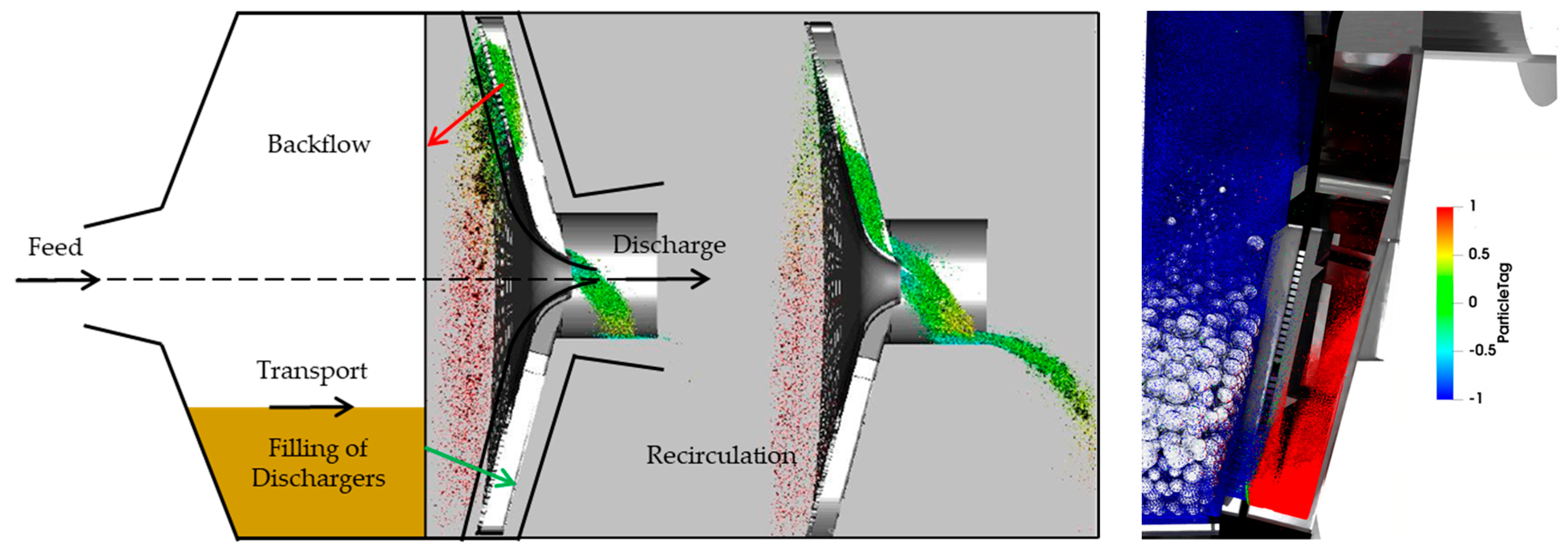
Latchireddi’s [32] intensive research has identified key inefficiencies in grinding circuits. One significant issue highlighted is the phenomenon of flow-back, inherent to conventional pulp lifter designs – Radial and Curved types. These designs are particularly problematic in mill running in closed circuit with cyclones or screens that handle a large volume of slurry—cases which circulating loads reach 400%-500%. The structural geometry of these pulp lifters ensures continuous contact between the slurry and the grate until discharge is complete, thereby making flow-back inevitable [32] as shown on Figure 20a.
The maximum flow that a pulp lifter assembly has to handle is the flow coming through the grates, at any hold up, and it can be estimated with grate-only discharge configuration, which is the benchmark for any alternative discharge assembly. The degree of deviation indicates the inefficiency involved in the pulp lifter discharge system. Based on this concept, Latchireddi conducted test work on a pilot scale to assess the performance of various arrangement correlating fractional hold-up with discharge rate for distinct designs.
The experiments revealed that load carrying capacity of the pulp lifters is more important than the opening area for a successful evacuation as can be seen on Figure 19a where “Large”, “Medium” and “Small” refers to the pulp lifter size mentioned as ratio of discharger to the mill length (Table 2).
Figure 19.
(a) Performance comparison of different sizes of Radial Pulp Lifters (RPL), (b) Performance comparison of different pulp lifter designs.
Figure 19.
(a) Performance comparison of different sizes of Radial Pulp Lifters (RPL), (b) Performance comparison of different pulp lifter designs.
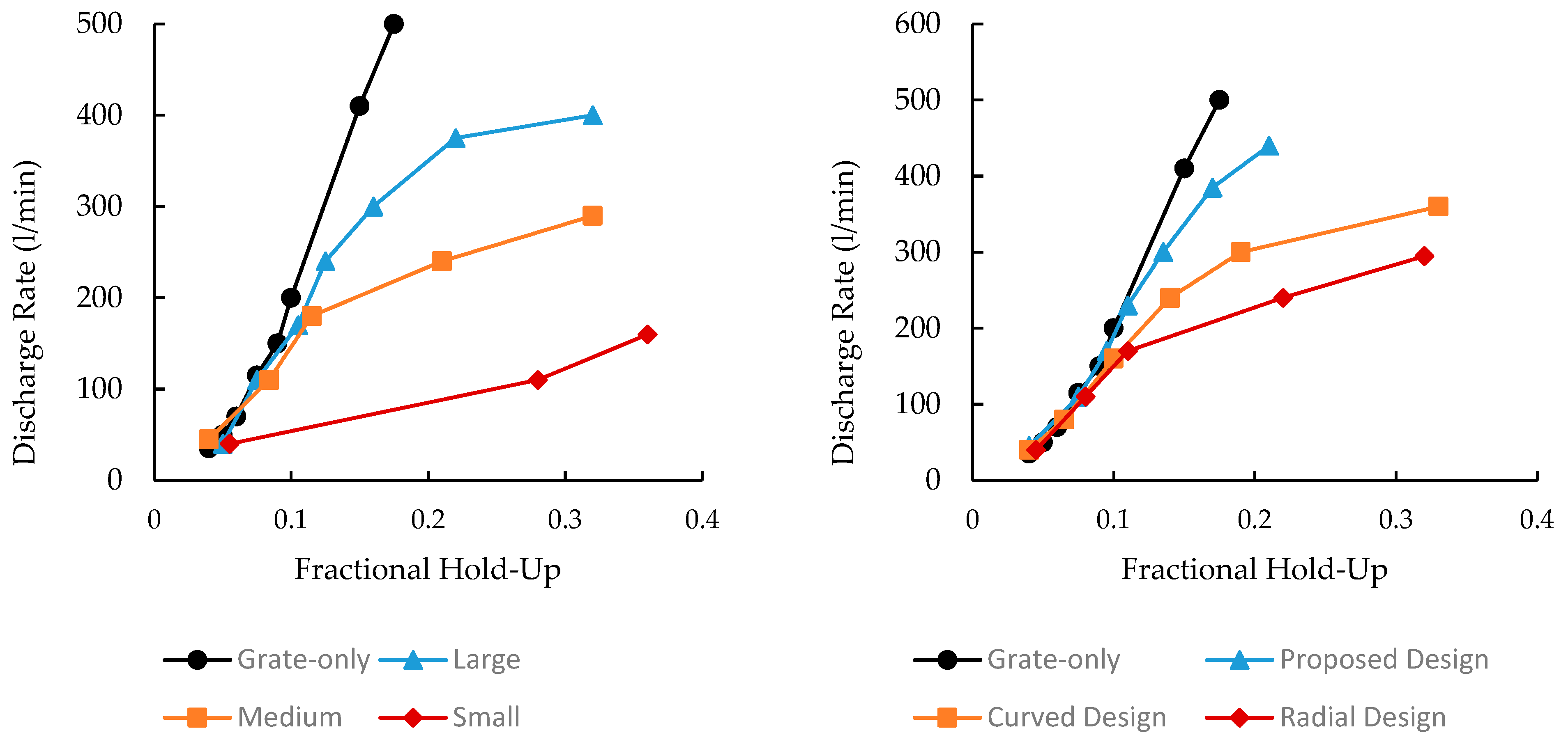
The flow capacity of curved pulp lifters was found to be always higher than the radial type which as observed earlier by Latchireddi and Morrel [33] and Burgess [34].
The inefficiency of conventional designs is attributed to size, carry-over, and mainly, the flow-back.
Figure 20.
(a) Flow-back process common to conventional discharge system. (b) Detail of the new discharger design which segregate materials and prevents recirculation inside the mill.
Figure 20.
(a) Flow-back process common to conventional discharge system. (b) Detail of the new discharger design which segregate materials and prevents recirculation inside the mill.
The flow-back phenomenon in grinding mills results not only in the formation of slurry pools but also significantly increases the presence of critical-sized particles within the mill in the case of AG and SAG mills. The negative effects of this flow-back are extensive and include energy waste, as energy is consumed to reprocess particles that have already reached the desired size but flow back through the grate. Industrial observations have quantified that such inefficiencies can reduce mill capacity by 10-35%, illustrating the significant impact of flow-back on mill performance [32].
To address these inefficiencies, a novel discharge system was developed, tested and implemented, specifically designed to eliminate the flow-back process and conserve energy that would otherwise be expended in vain. This system incorporates a system of deflectors that prevent direct contact of the slurry with the grate apertures during evacuation, guaranteeing that no material returns to the mill chamber (Figure 20b). By halting the recirculation of particles, the pulp lifting mechanism directs all available energy towards breaking new particles. Consequently, this enhances overall mill performance and reduces energy consumption by ensuring that the energy is used effectively and not wasted on redundant processing.
3.2. Dead Zone
Through numerical methods that merge methodologies presented in this research to mirror the real-world dynamics of a mill operating at industrial scale, the author has unveiled a critical relationship between increased filling charges and the formation of dead zones within the mill as shown on Figure 21. These dead zones are characterized by their notably material low relative velocity, rendering them incapable of generating the requisite energy to match the hardness of the minerals under processing. It has been found that these dead zones can constitute up to 32% of the mill’s charge by volume when the filling charges exceed 28%. In terms of weight, this proportion may escalate even further, as the central areas of the charge tend to accumulate deformed grinding balls and scats, resulting in a densely compacted core of material that is significantly heavier with bulk density exceeding 6500 kg/m3.
This compacted central mass creates a scenario where slurry cannot permeate due to a lack of porosity, and despite its inactivity towards ore size reduction, it draws substantial power. The mill expends a massive amount of torque just to maintain this non-productive charge in such position, significantly diminishing its performance. Addressing this inefficiency necessitates the removal of such non-useful material from the equipment, which is pivotal for transitioning to an energy-efficient milling system. This process not only alleviates the unnecessary power draw but also enhances the overall operational efficacy of the mill generating effective volume and higher drop height for the balls.
In the industry, there is a prevailing belief that higher power draw is synonymous with increased throughput, suggesting a positive and even linear relationship between these two variables. However, extensive studies challenge this assumption, revealing that the relationship between power draw and throughput does not consistently maintain a positive relation across the entire operational spectrum nowadays. Research has identified a critical juncture where the rate of increase in specific input energy is higher than the rate of increase in specific impact energy, particularly as the mill size increases and is operated with excessive filling charge. This discrepancy becomes more pronounced in larger mills, indicating that the efficiency gains expected from merely increasing power are not realized.
The high inefficiencies in the tumbling mills, which are prevalent in mines worldwide, can largely be attributed to the excessive accumulation of materials within the mill chamber. This includes an excess of critical size balls, scats and slurry. Such accumulation not only contributes to suboptimal milling conditions but also underscores a significant loss in energy efficiency. By decreasing the amount of non-contributive material in the mill, it becomes possible to enhance the milling process’s efficiency, pointing towards a more sustainable approach in mineral processing operations. This method represents a disruptive shift in optimizing mill performance, focusing on operational adjustments rather than simply increasing power input.
4. Discussion
The efficacy of the proposed discharge system is underscored not only by its ability to facilitate a superior hydraulic gradient but also by its capacity to streamline the flow of materials through the mill. This system adeptly assists in the elimination of scats—coarser materials which, if accumulated, can severely impede the milling process. The efficient removal of these materials ensures the liberation of the mill’s internal volume for active grinding, thus preventing the occupation of this critical space by materials that do not contribute to the grinding process.
Moreover, a pivotal feature of the grate discharge configuration is the increased fall height between the shoulder and the toe of the charge. This enhanced drop height amplifies the impact forces during collisions between the grinding media, thereby facilitating a more effective comminution per collision event. Such dynamics ensure fine and uniform particle sizes, which is essential for downstream process.
Additionally, the grate discharge mill curtails the prevalence of ’dead zones’—regions within the mill where the motion of the balls is markedly reduced, leading to significant torque consumption without corresponding contributions to particle size reduction. These zones, prevalent in typical overflow mills, can constitute approximately 32% of the mill’s charge volume, markedly diminishing the mill’s operational efficiency. In stark contrast, the grate discharge setup substantially reduces these non-contributive areas, ensuring that a larger proportion of the energy input into the mill is directly utilized for particle size reduction.
The new discharge configuration in combination with new operational methodology significantly boost milling performance, even with a reduced count of grinding media, showcasing the superior efficiency of mills operating with the Energy Efficient Pulp Lifting System in optimizing energy consumption and enhancing both throughput and particle size reduction outcomes. Through such innovation, the design and functionality of grate discharge mills demonstrate a profound capability to transcend conventional milling limitations, paving the way for more refined and energy-efficient milling processes.
Moreover, these simulations are computationally expensive due to the sheer scale and complexity involved in accurately modeling such detailed interactions. The use of GPU-based computational models was pivotal in managing these demands. GPUs, with their parallel processing capabilities, are particularly adept at handling large datasets and executing parallel operations rapidly, which is essential for the DEM (Discrete Element Method) and SPH (Smoothed Particle Hydrodynamics) simulations used in this study. This technological approach allowed us to perform high-fidelity simulations that would have been prohibitively time-consuming and expensive with traditional CPU-based systems. The GPU architecture excels in tasks that can be broken down into smaller concurrent processes, making it an ideal choice for the particle-based modeling techniques where thousands of individual calculations need to be performed simultaneously.
Author Contributions
Wallace S. Soares: Conceptualization, Data curation, Formal analysis, Investigation, Methodology, Software, Writing – original draft. Nicolin Govender: Data curation, Investigation, Software, Writing - review. All authors have read and agreed to the published version of the manuscript.
Acknowledgments
We gratefully acknowledge the support of AIA Engineering and Vega Industries for their significant technical contributions to this project. AIA and Vega, along with its partner, hold the patent for the product investigated in this study. Their openness in sharing the design and operating conditions of the product has enabled a thorough investigation of its performance and how it benefits the mining industry.
Conflicts of Interest
The authors declare no conflicts of interest.
Abbreviations
The following abbreviations are used in this manuscript:
| MDPI | Multidisciplinary Digital Publishing Institute |
| DOAJ | Directory of open access journals |
| DEM | Discrete element method |
| CFD | Computational Fluid Dynamics |
| SPH | Smooth particle hydrodynamics |
| BM | Ball mill |
| AG | Autogenous mill |
| SAG | Semi-autogenous mill |
| PSD | Particle size distribution |
| HC | Hydrocyclone |
| O/F | Overflow |
| U/F | Underflow |
| GD | Grate discharge |
| RPL | Radial pulp lifting system |
| CPL | Curved pulp lifting system |
| EEPL™ | Energy Efficient Pulp Lifting System™ |
| PSD | Particle size distribution |
| tph | Tonnage per hour |
| kW | Kilowatt |
| kWh | Kilowatt-hour |
| BWI | Bond work index |
| DCS | Distributed control system |
References
- J. J. Monaghan. “Simulating free surface flows with SPH”. Journal of Computational Physics 1994, 110, 399–406. [CrossRef]
- R. Vignjevic and J. Campbell. “Review of Development of the Smooth Particle Hydrodynamics (SPH) Method”. In: Predictive Modeling of Dynamic Processes: A Tribute to Professor Klaus Thoma. Ed. by Stefan Hiermaier. Boston, MA: Springer US, 2009, pp. 367–396. ISBN: 978-1- 4419-0727-1.
- R. Fatehi and M. T. Manzari. “Error estimation in smoothed particle hydrodynamics and a new scheme for second derivatives”. Computers and Mathematics with Applications 2011, 61, 482–498. [CrossRef]
- L.D. Libersky and A.G. Petschek. “Smooth particle hydrodynamics with strength of materials”. In: Advances in the Free-Lagrange Method Including Contributions on Adaptive Gridding and the Smooth Particle Hydrodynamics Method. Berlin, Heidelberg: Springer, 1991, pp. 248–257.
- H. Takeda, S. M. Miyama, and M. Sekiya. “Numerical Simulation of Viscous Flow by Smoothed Particle Hydrodynamics”. In: Progress of Theoretical Physics 92.5 (Nov. 1994), pp. 939–960.
- A. Ferrari, M. Dumbser, E. F. Toro, and A. Armanini. “A new 3D parallel SPH scheme for free surface flows”. Computers and Fluids 2009, 38, 1203–1217. [CrossRef]
- S. Kulasegaram, J. Bonet, R. W. Lewis, and M. Profit. “A variational formulation based contact algorithm for rigid boundaries in two-dimensional SPH applications”. Computational Mechanics 2004, 33, 316–325. [CrossRef]
- R. A. Gingold and J.J. Monaghan. “Smoothed particle hydrodynamics: theory and application to non-spherical stars”. Monthly Notices of the Royal Astronomical Society 1977, 181, 375–389. [CrossRef]
- R.H. Cole and I. Weller. “Underwater explosions and their application in simulations”. Journal of Fluid Dynamics 1977, 34, 214–227.
- A. V. Potapov, M. L. Hunt, and C. S. Campbell. “Liquid-solid flows using smoothed particle hydrodynamics and the discrete element method”. Powder Technology 2001, 116, 204–213. [CrossRef]
- J.M. Dominguez, G. Fourtakas, C. Altomare, R.B. Canelas, A. Tafuni, O. Garcia- Feal, et al., DualSPHysics: from fluid dynamics to multiphysics problems. Comput. Part. Mech. 2022, 9, 867–895. [CrossRef]
- A.J.C. Crespo, M. Gomez-Gesteira, R.A. Dalrymple, Boundary conditions generated by dynamic particles in SPH methods. CMC Comp. Mater. Continua. 2007, 5, 173–184.
- A. English, J.M. Dominguez, R. Vacondio, A.J.C. Crespo, P.K. Stansby, S.J. Lind, et al., Modified dynamic boundary conditions (mDBC) for general-purpose smoothed particle hydrodynamics (SPH): application to tank sloshing, dam break and fish pass problems. Comput. Part. Mech. 2022, 9, 911–925.
- B. Leimkuhler, C. Matthews (Eds.), Molecular Dynamics: With Deterministic and Stochastic Numerical Methods, Springer International Publishing, Cham, 2015, pp. 1–51.
- A.N. Parshikov, S.A. Medin, I.I. Loukashenko, V.A. Milekhin, Improvements in SPH method by means of interparticle contact algorithm and analysis of perforation tests at moderate projectile velocities. Int. J. Impact Eng. 2000, 24, 779–796. [CrossRef]
- J.J. Monaghan, A. Kos, Solitary waves on a Cretan beach. J. Waterway Port Coast. Ocean Eng. Asce. 1999, 125, 145–154. [CrossRef]
- F.Z. Xie, W.W. Zhao, D.C. Wan, MPS-DEM coupling method for interaction between fluid and thin elastic structures, Ocean Eng. 236 (2021).
- N. Govender, Study on the effect of grain morphology on shear strength in granular materials via GPU based discrete element method simulations. Powder Technol. 2021, 387, 336–347. [CrossRef]
- K. Kildashti, K.J. Dong, B. Samali, Q.J. Zheng, A.B. Yu, Evaluation of contact force models for discrete modelling of ellipsoidal particles. Chem. Eng. Sci. 2018, 177, 1–17. [CrossRef]
- L. Liu, J. Wu, S.Y. Ji, DEM-SPH coupling method for the interaction between irregularly shaped granular materials and fluids, Powder Technol. 400 (2022.
- Z.H. Shen, G. Wang, D.R. Huang, F. Jin, A resolved CFD-DEM coupling model for modeling two-phase fluids interaction with irregularly shaped particles, J. Comput. Phys. 448 (2022).
- N. Govender, R.K. Rajamani, S. Kok, D.N. Wilke, Discrete element simulation of mill charge in 3D using the BLAZE-DEM GPU framework. Miner. Eng. 2015, 79, 152–168. [CrossRef]
- N. Govender, A DEM study on the thermal conduction of granular material in a rotating drum using polyhedral particles on GPUs, Chem. Eng. Sci. 252 (2022).
- B. Smeets, T. Odenthal, S. Vanmaercke, H. Ramon, Polygon-based contact description for modeling arbitrary polyhedra in the discrete element method. Comput. Methods Appl. Mech. Eng. 2015, 290, 277–289. [CrossRef]
- R. Venugopal, 3D simulation of charge motion in tumbling mills by the discrete, Powder Technol. 115 (2001) 157–166.
- N. Govender, D.N. Wilke, C.-Y. Wu, R. Rajamani, J. Khinast, B.J. Glasser, Large-scale GPU based DEM modeling of mixing using irregularly shaped particles. Adv. Powder Technol. 2018, 29, 2476–2490. [CrossRef]
- N. Govender, D.N. Wilke, P. Pizette, N.E. Abriak, A study of shape non-uniformity and poly-dispersity in hopper discharge of spherical and polyhedral particle systems using the Blaze-DEM GPU code, Appl. Math. Comput. 2018.
- S. Morrell. “Power draw of wet tumbling mills and its relationship to charge dynamics - Part 1: a continuum approach to mathematical modelling of mill power draw.” In: Transactions of the Institution of Mining and Metallurgy, Section C: Mineral Processing and Extractive Metallurgy 105 (1996), pp. A9–A14.
- T.J. Napier-Munn et al. “Mineral Comminution Circuits: Their Operation and Optimization”. In: Julius Kruttschnitt Mineral Research Centre, The University of Queensland (1996).
- H. Wendland, Piecewise polynomial, positive definite and compactly supported radial functions of minimal degree. Adv. Comput. Math. 1995, 4, 389–396. [CrossRef]
- M. Capece, E. Bilgili, R. Dave, Insight into first-order breakage kinetics using a particle-scale breakage rate constant, Chem. Eng. Sci. 117 (2014) 318–330.
- Latchireddi, S. R., Morrell, S. Influence of discharge pulp lifter design on slurry flow in mills. Paper presented at the Mining Millennium 2000 Conference, Toronto, Canada (2000, March).
- Latchireddi, S., Morrell, S. (1997). A laboratory study of the performance characteristics of mill pulp lifters. Minerals Engineering, 10(11), 1221-1231.
- Burgess, D. , 1989. High or low aspect - which one? SAG Milling Conference (Ed. Stockton, N.D.), Murdock University: 132-170.
- Cleary, P. W., Sinnott, M., & Morrison, R. (2006). Prediction of slurry transport in SAG mills using SPH fluid flow in a dynamic DEM based porous media. Minerals Engineering, 19(15), 1517-1527.
- Cleary, P. W. , & Morrison, R. D. (2012). Prediction of 3D slurry flow within the grinding chamber and discharge from a pilot scale SAG mill. *Minerals Engineering, 39, 184-198.
- Cleary, P. W., Morrison, R. D., & Sinnott, M. D. Prediction of slurry grinding due to media and coarse rock interactions in a 3D pilot SAG mill using a coupled DEM+SPH model. Minerals Engineering, 2020, 157, 106614.
- Cleary, P. W. , Cummins, S. J., & Sinnott, M. D. Advanced comminution modelling: Part 2-Mills. Applied Mathematical Modelling, 2020, 89, 640–670. [Google Scholar]
Figure 1.
Flow diagram of coupling scheme between DEM and MLMs.

Figure 2.
Polyhedron modeling method in DEM; (a) Triangles connected with similar orientation; (b) Triangles connected and with same orientation are merged creating feature edges and vertex; (c) Definition of a unique polygon faces including the center point and the normal direction.
Figure 2.
Polyhedron modeling method in DEM; (a) Triangles connected with similar orientation; (b) Triangles connected and with same orientation are merged creating feature edges and vertex; (c) Definition of a unique polygon faces including the center point and the normal direction.
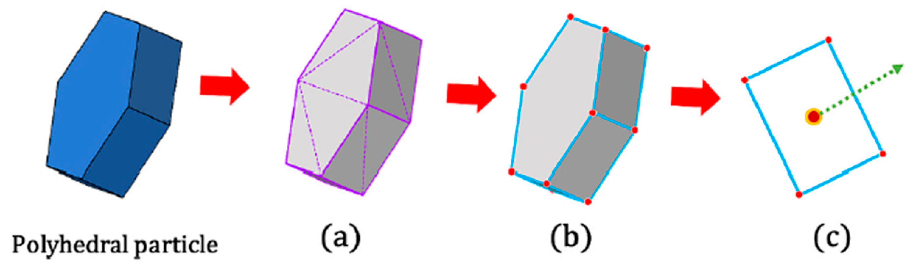
Figure 3.
Broad phase contact detection and detailed contact resolution for polyhedral particles: (a) Broad phase – Contact detection; (b) Intermediate phase – Contact resolution; (c) Narrow phase – Detail contact resolution.
Figure 3.
Broad phase contact detection and detailed contact resolution for polyhedral particles: (a) Broad phase – Contact detection; (b) Intermediate phase – Contact resolution; (c) Narrow phase – Detail contact resolution.
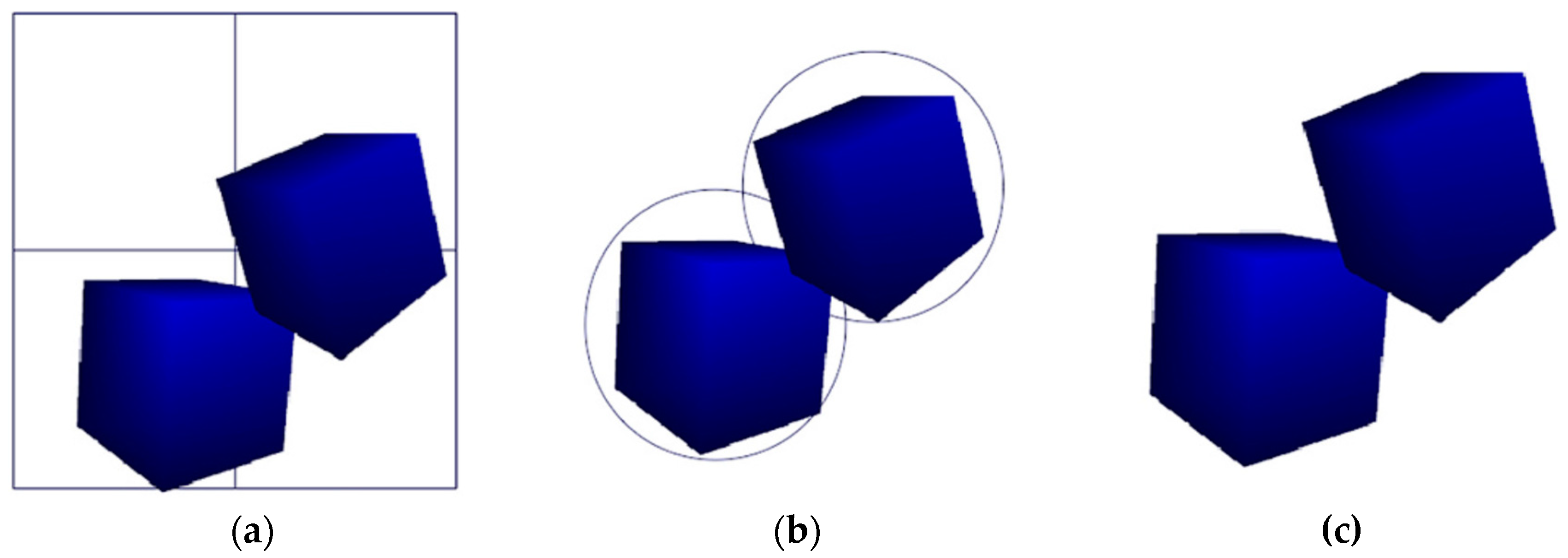
Figure 4.
The contact solution of two polyhedral particles (P1, P2) based on the overlap volume; (a) The convex hull is constructed to calculate the contact volume; (b) Contact volume; (c) The corresponding contact normal and particle forces are analyzed for each particle.
Figure 4.
The contact solution of two polyhedral particles (P1, P2) based on the overlap volume; (a) The convex hull is constructed to calculate the contact volume; (b) Contact volume; (c) The corresponding contact normal and particle forces are analyzed for each particle.
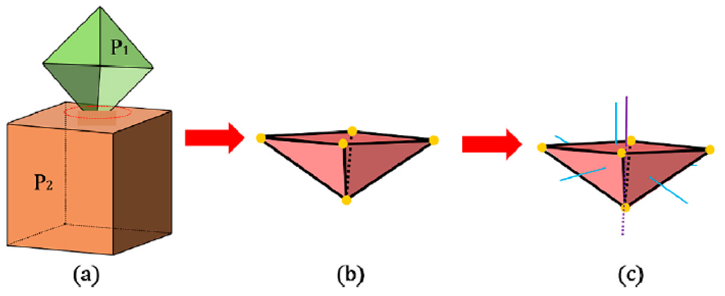
Figure 5.
Diagram of the free-surface flow interacting with polyhedral particles modelled in DualSPHysics and Blaze-DEM.
Figure 5.
Diagram of the free-surface flow interacting with polyhedral particles modelled in DualSPHysics and Blaze-DEM.
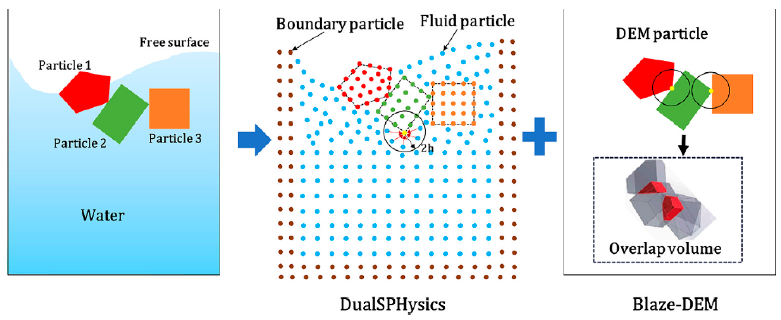
Figure 6.
Flowchart of the coupling of DualSPHysics and Blaze-DEM.
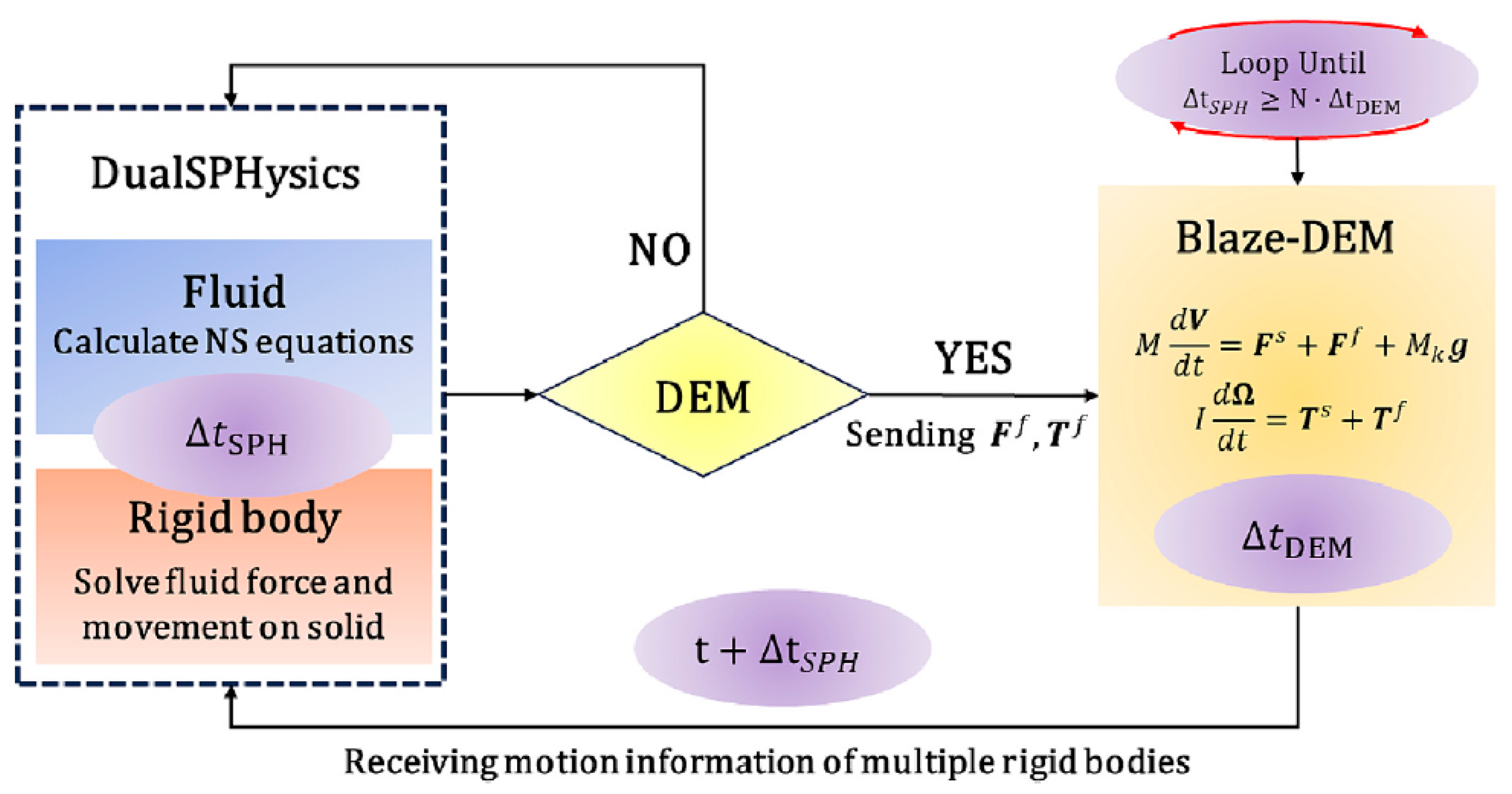
Figure 7.
Particle size distributions of mill discharge and hydrocyclone overflow in the baseline scenario: BM with overflow configuration.
Figure 7.
Particle size distributions of mill discharge and hydrocyclone overflow in the baseline scenario: BM with overflow configuration.
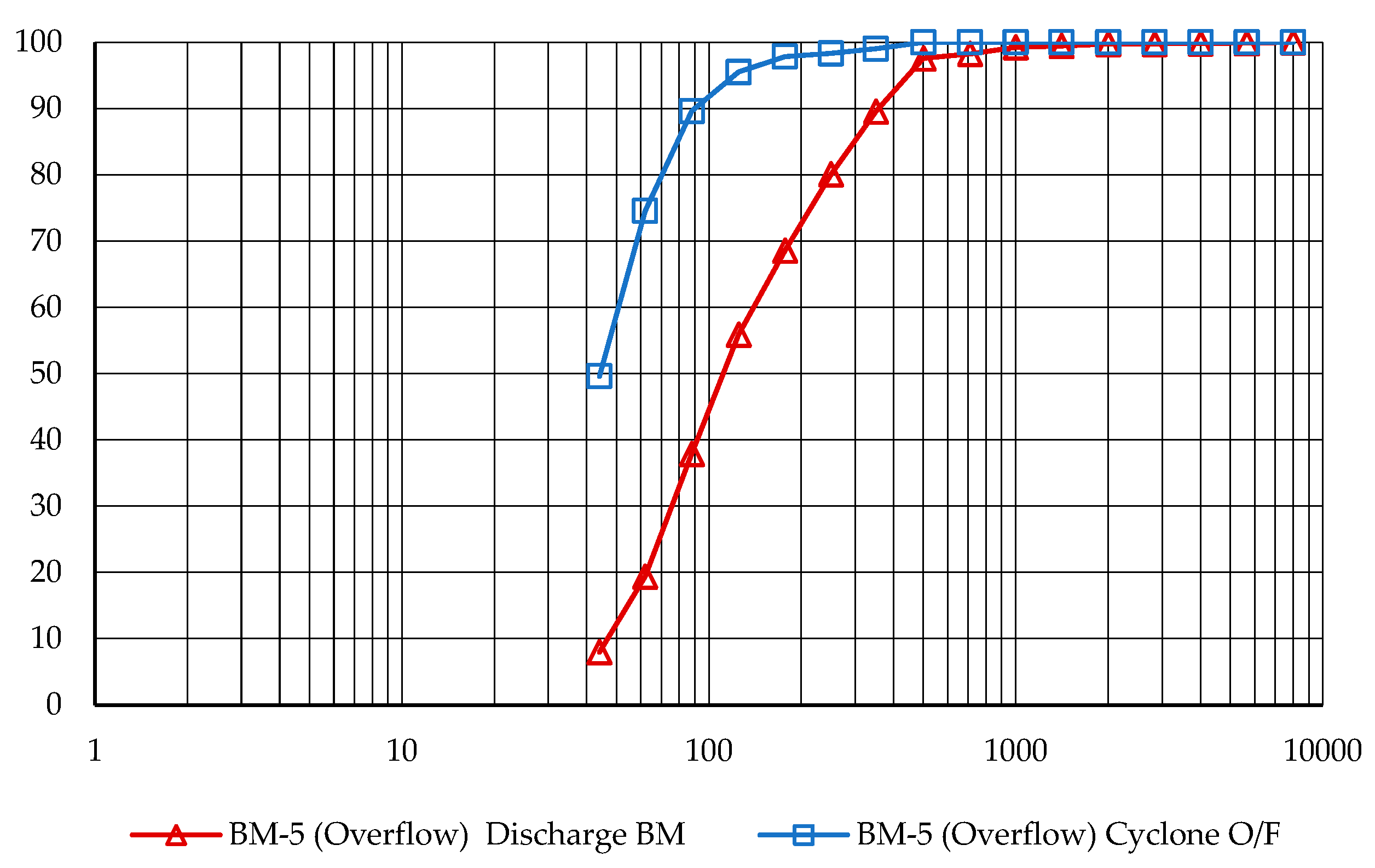
Figure 8.
Power output of BM-5 operating under standard conditions: data sourced from Plant Control Center.
Figure 8.
Power output of BM-5 operating under standard conditions: data sourced from Plant Control Center.
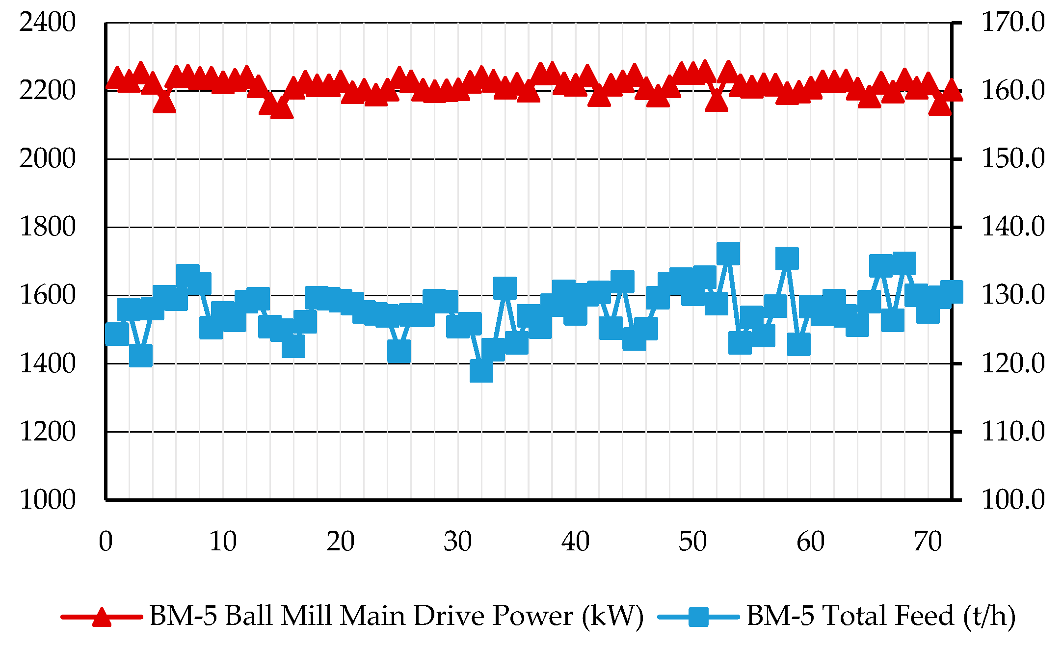
Figure 9.
Power output of BM-5 operating under standard conditions: real-time data from plant control center vs. model response.
Figure 9.
Power output of BM-5 operating under standard conditions: real-time data from plant control center vs. model response.
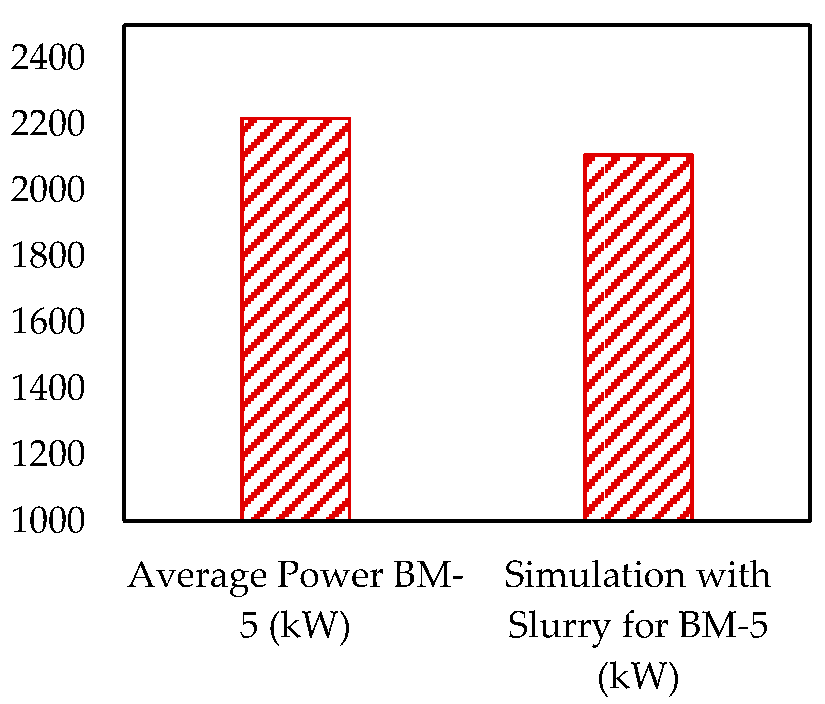
Figure 10.
Comparative particle size distributions of ball mill discharge: Overflow vs. Grate Discharge arrangements.
Figure 10.
Comparative particle size distributions of ball mill discharge: Overflow vs. Grate Discharge arrangements.
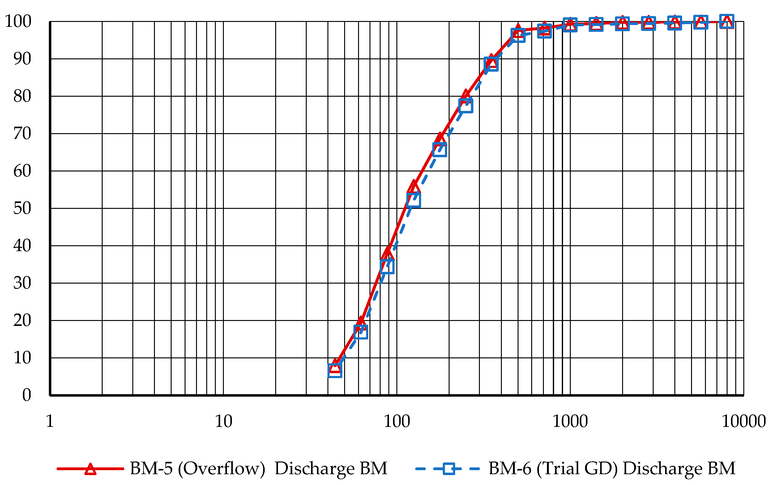
Figure 11.
Comparison of Particle Size Distributions in Hydrocyclone Overflow: Overflow vs. Grate Discharge Arrangements.
Figure 11.
Comparison of Particle Size Distributions in Hydrocyclone Overflow: Overflow vs. Grate Discharge Arrangements.
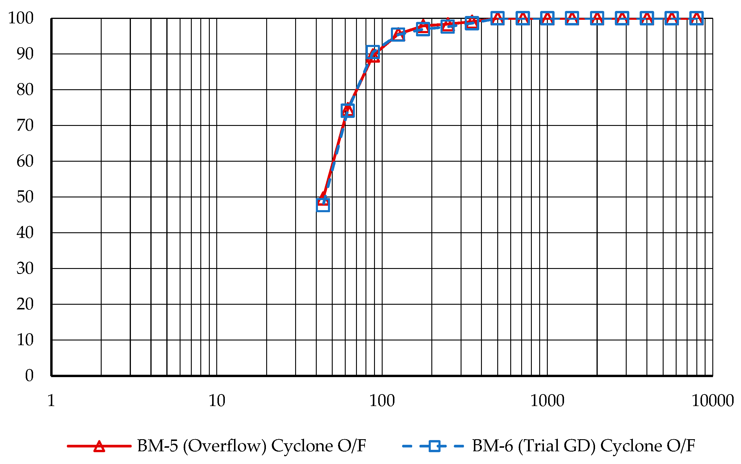
Figure 12.
(a) Energy spectra of standard (SlurryOF) and trial scenarios (SlurryGD). (b) Flow though the chambers till ready steady-state condition.
Figure 12.
(a) Energy spectra of standard (SlurryOF) and trial scenarios (SlurryGD). (b) Flow though the chambers till ready steady-state condition.
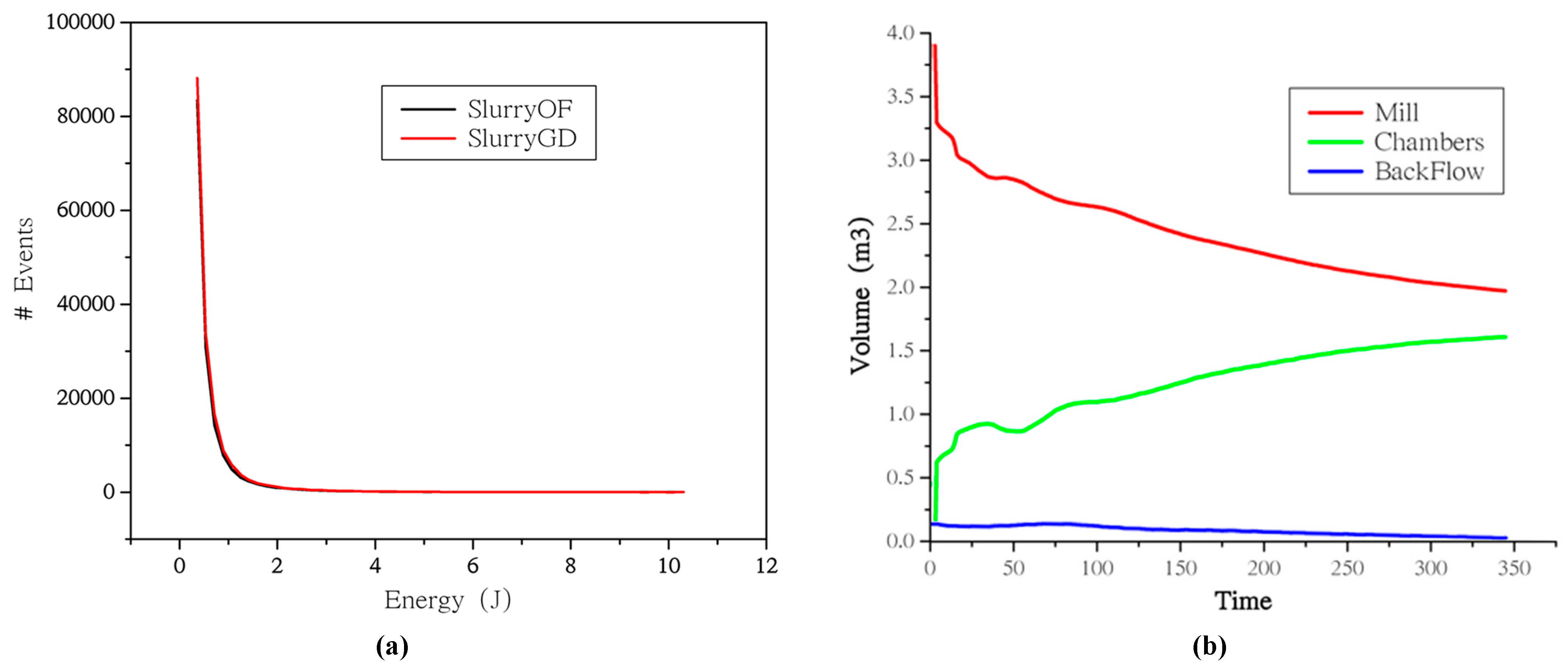
Figure 13.
Power output of BM-6 running with modified design: data sourced from Plant Control Center.
Figure 13.
Power output of BM-6 running with modified design: data sourced from Plant Control Center.
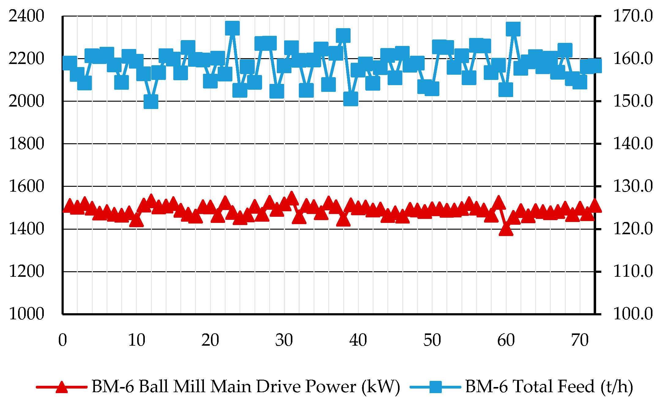
Figure 14.
Charge distribution within mill chamber for an overflow discharge type. Showcasing the theoretical ideal ore-ball ratio: (a) Standstill condition – slurry settled; (b) Steady-state achieved following the fourth revolution in the simulation.
Figure 14.
Charge distribution within mill chamber for an overflow discharge type. Showcasing the theoretical ideal ore-ball ratio: (a) Standstill condition – slurry settled; (b) Steady-state achieved following the fourth revolution in the simulation.
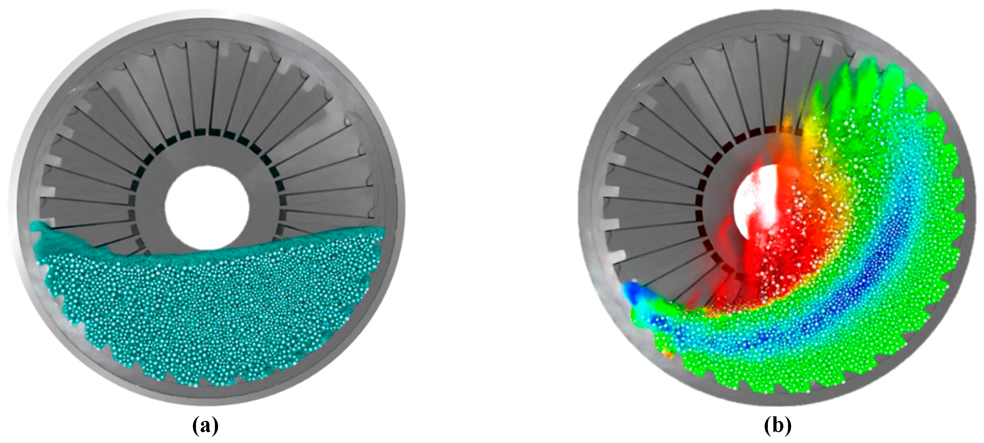
Figure 15.
Charge distribution within mill chamber for an overflow discharge type. Showcasing : (a) Standstill condition – slurry settled; (b) Steady-state achieved following the fourth revolution in the simulation.
Figure 15.
Charge distribution within mill chamber for an overflow discharge type. Showcasing : (a) Standstill condition – slurry settled; (b) Steady-state achieved following the fourth revolution in the simulation.
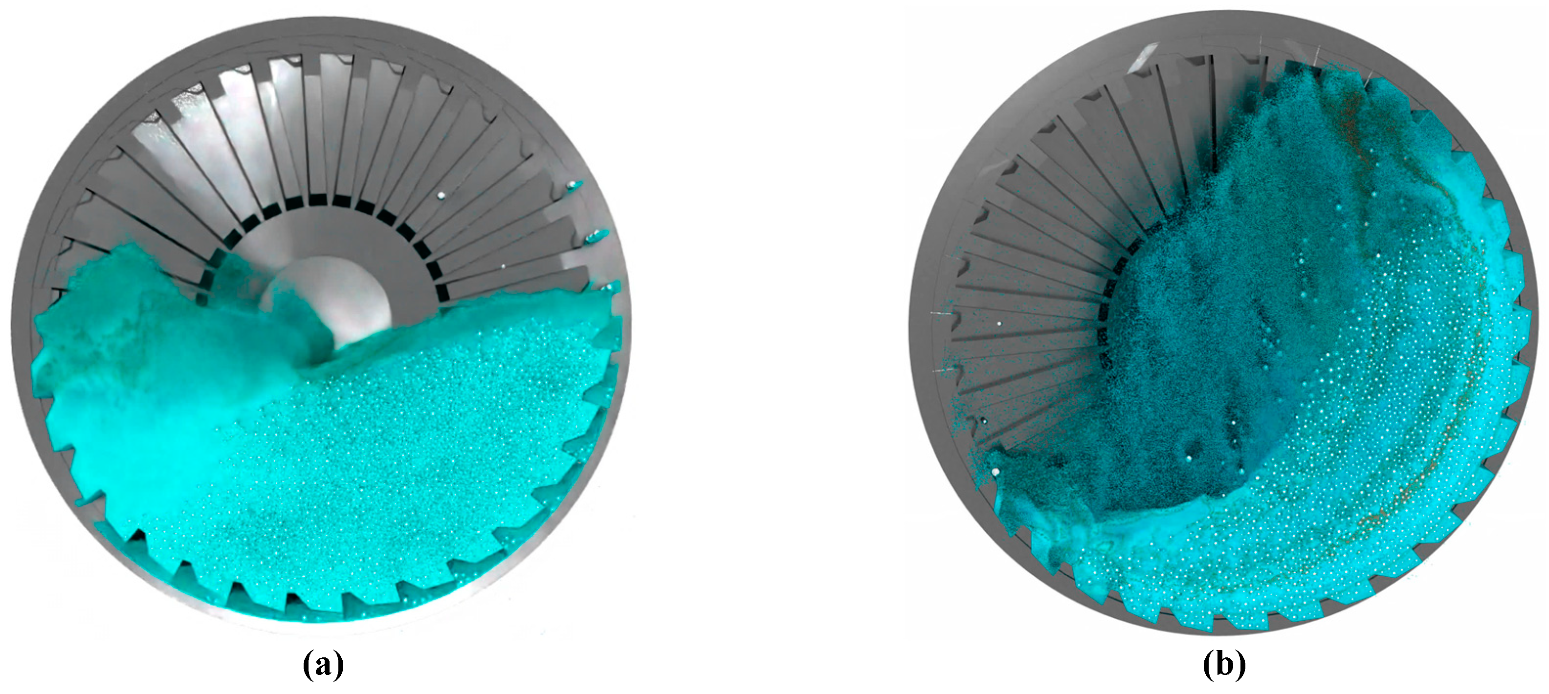
Figure 16.
Charge distribution within mill chamber for an overflow discharge type. Showcasing : (a) Standstill condition – slurry settled; (b) Steady-state achieved following the fourth revolution in the simulation.
Figure 16.
Charge distribution within mill chamber for an overflow discharge type. Showcasing : (a) Standstill condition – slurry settled; (b) Steady-state achieved following the fourth revolution in the simulation.
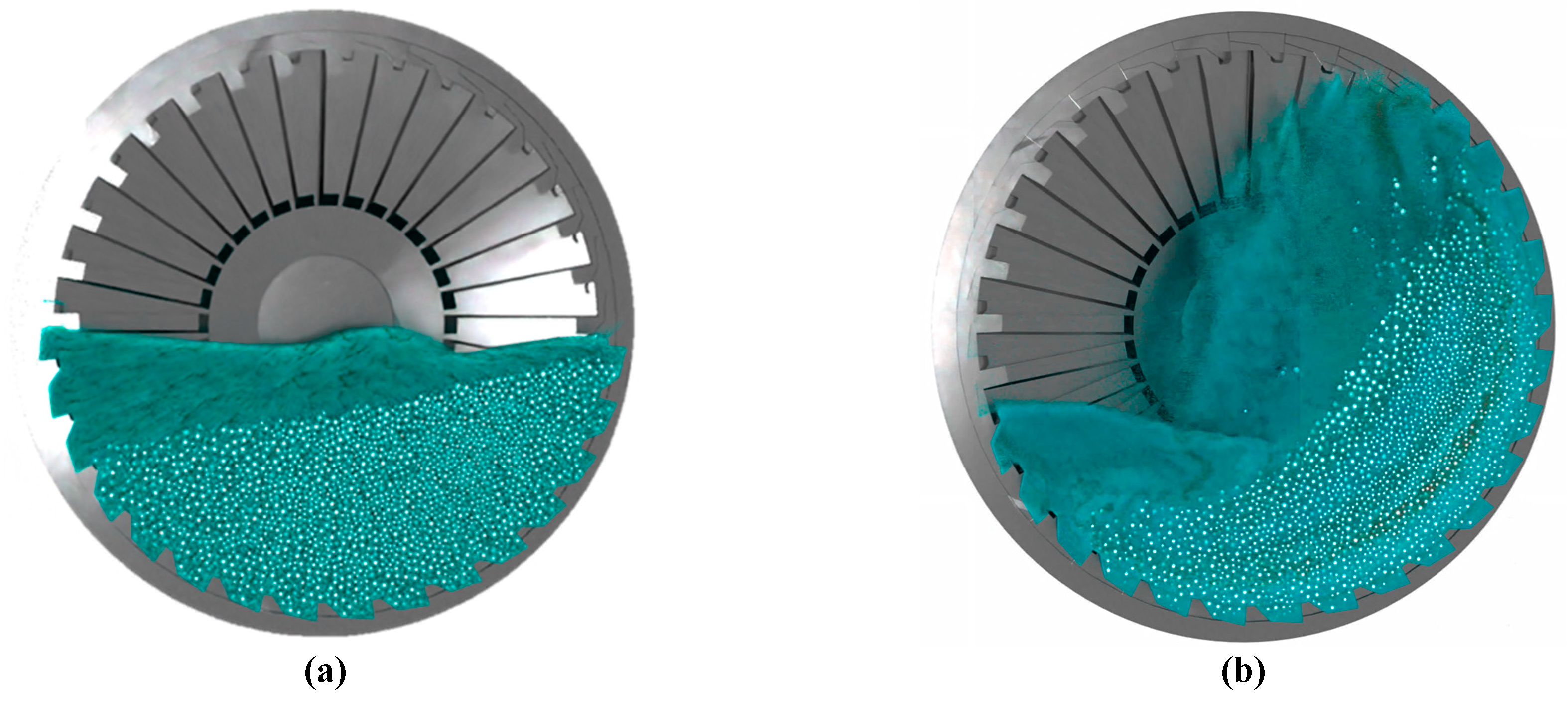
Figure 17.
Charge distribution within mill chamber for a non-conventional grate discharge arrangement. Showcasing : (a) Standstill condition – slurry settled – inside view; (b) Standstill condition – slurry settled – outside view.
Figure 17.
Charge distribution within mill chamber for a non-conventional grate discharge arrangement. Showcasing : (a) Standstill condition – slurry settled – inside view; (b) Standstill condition – slurry settled – outside view.
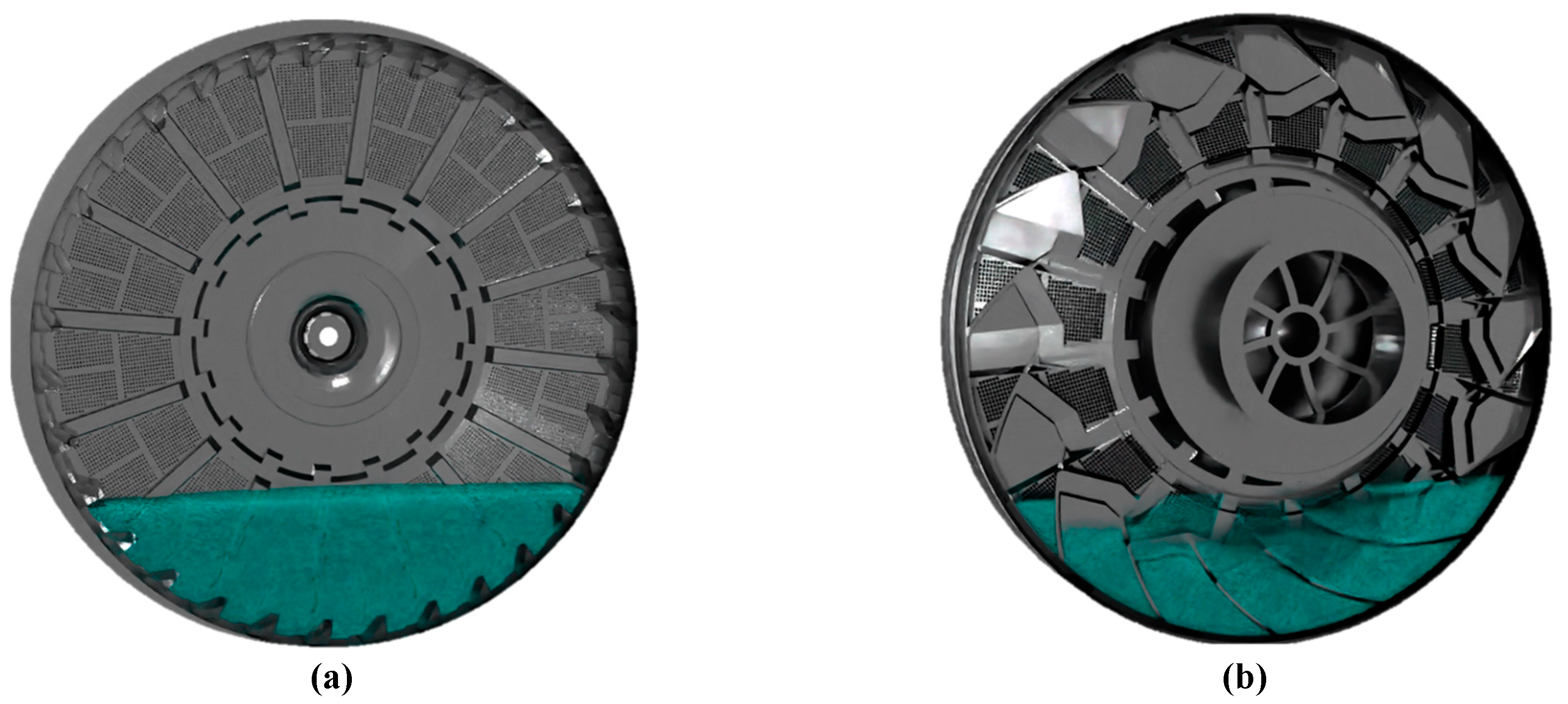
Figure 18.
Charge motion: (a) inside view; (b) outside view.
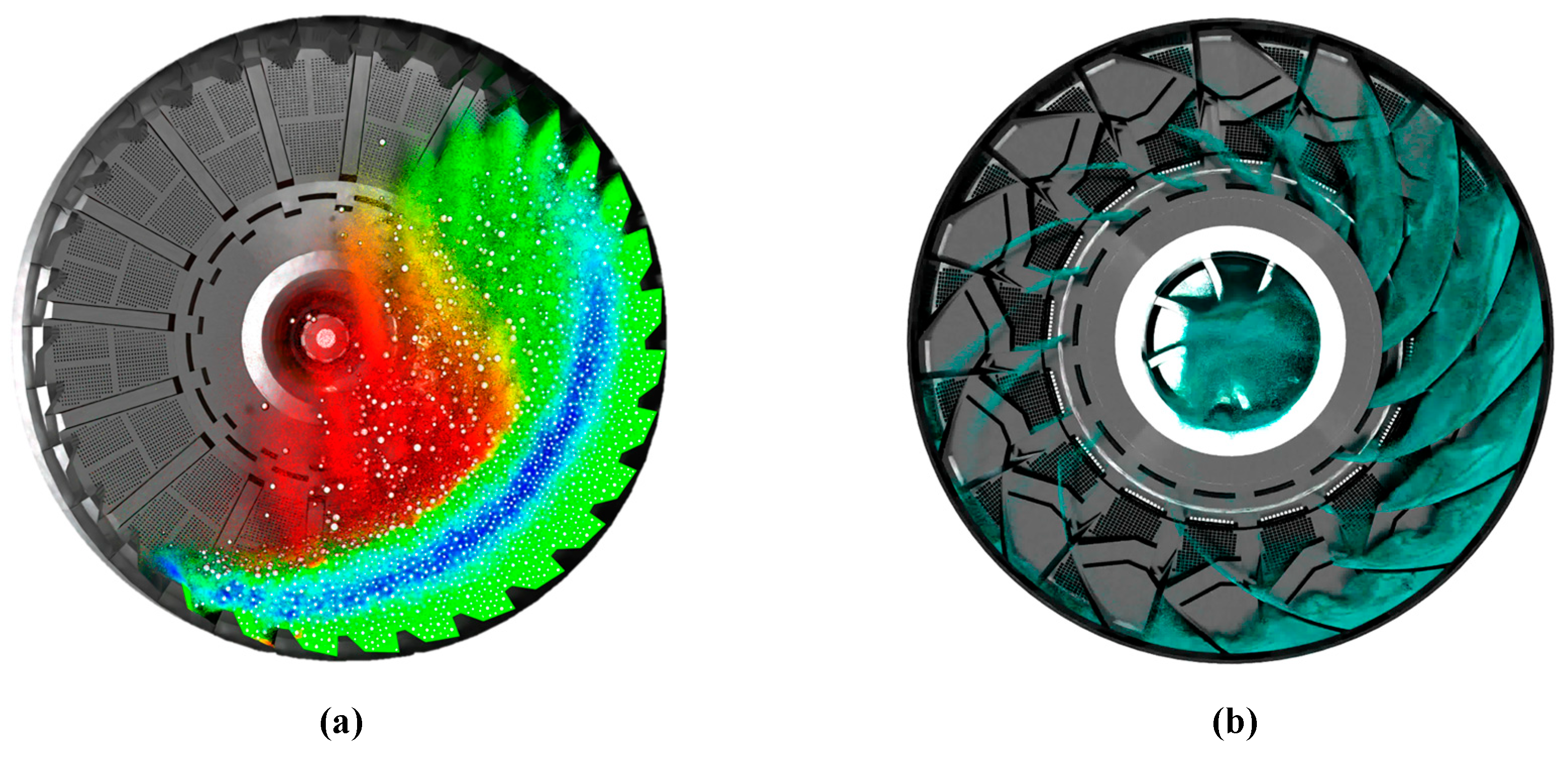
Figure 21.
Comparative visualization of dead zones in mill discharge systems: (a), (c) and (e) show an overflow ball mill and (b), (d) and (e) a grate discharge ball mill, respectively, with dead zones highlighted in various shades of blue. Panels (c) and (d) provide side views, while (e) and (f) cross-section interior view with the charge in steady-state, clearly illustrating the distribution and extent of low-activity regions within the mill chambers, indicative of reduced grinding efficiency in these areas.
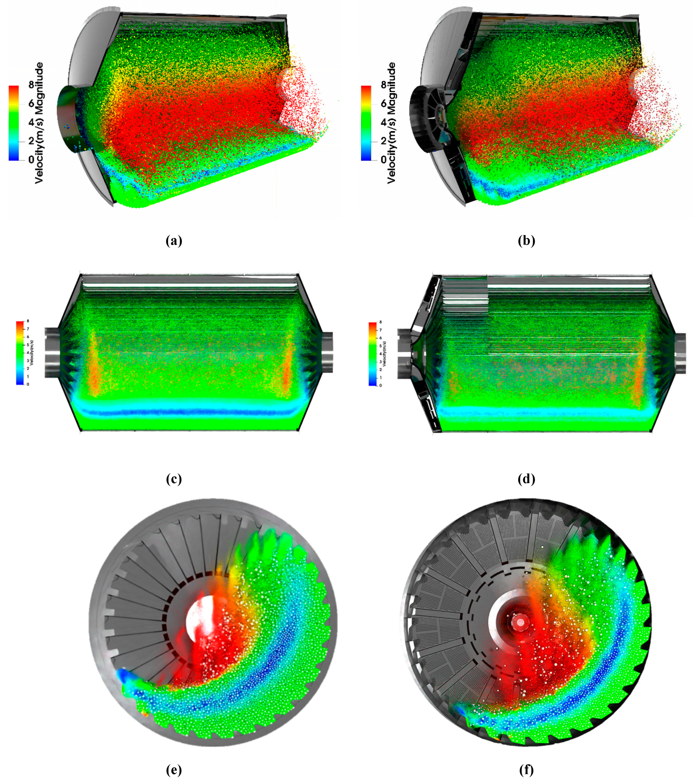

Table 1.
P80 values of mill discharge and cyclone overflow under overflow and grate discharge configurations.
Table 1.
P80 values of mill discharge and cyclone overflow under overflow and grate discharge configurations.
| Sample | BM-5 (Overflow) Discharge of BM | BM-6 (Trial GD) Discharge of BM | BM-5 (Overflow) Cyclone O/F | BM-6 (Trial GD)Cyclone O/F |
| A | 295.10 | 298.15 | 69.22 | 65.63 |
| B | 295.86 | 302.12 | 65.89 | 69.85 |
| C | 302.59 | 301.55 | 66.81 | 65.64 |
| D | 299.57 | 300.92 | 66.84 | 66.76 |
| E | 304.51 | 293.19 | 67.65 | 67.46 |
| F | 293.31 | 298.43 | 68.09 | 67.89 |
| G | 288.73 | 292.72 | 68.64 | 67.95 |
| H | 294.91 | 296.22 | 69.15 | 68.64 |
| I | 300.49 | 297.74 | 69.69 | 69.12 |
| J | 286.50 | 296.78 | 70.59 | 70.61 |
1 Each sample was tentatively weighed at 10 kg for uniformity and representativeness of the analysis. 2 All values refer to the 80% cumulative passing size, and the unit of measurement is millimeters (mm).
Table 2.
Sizing Criteria.
| Pulp Lifter Size | Percent Ratio |
| Small | 3.7 |
| Medium | 6.8 |
| Large | 9.9 |
1 Percent ratio = [(Pulp Lifter Width/Mill Length)*100].
Disclaimer/Publisher’s Note: The statements, opinions and data contained in all publications are solely those of the individual author(s) and contributor(s) and not of MDPI and/or the editor(s). MDPI and/or the editor(s) disclaim responsibility for any injury to people or property resulting from any ideas, methods, instructions or products referred to in the content. |
© 2025 by the authors. Licensee MDPI, Basel, Switzerland. This article is an open access article distributed under the terms and conditions of the Creative Commons Attribution (CC BY) license (http://creativecommons.org/licenses/by/4.0/).
Copyright: This open access article is published under a Creative Commons CC BY 4.0 license, which permit the free download, distribution, and reuse, provided that the author and preprint are cited in any reuse.


