
Submitted:
30 April 2025
Posted:
02 May 2025
You are already at the latest version
Abstract
Ocean-going vessels rely on marine diesel engines, referred to as the main engine, to carry the vessel’s load and ensure safe travel. These engines play a critical role, as their operation impacts all aspects of the vessel’s functionality. To meet increasing demands for extended run times while maintaining reliability, it is essential to address the risks of main engine failure. Previous studies have highlighted numerous accidents resulting from such failures. Consequently, the reliability of the main propulsion engine is a crucial component of safe vessel operation. This study addresses the lack of methodologies for predicting engine reliability using Failure Running Hours (FRH). A data-driven model has been developed based on information collected from marine engineers during on-board maintenance activities. Additionally, Fault Tree Analysis (FTA) is employed to calculate the reliability of individual sub-systems and the overall main propulsion engine. Findings reveal that the main propulsion engine’s reliability declines to 0% at approximately 900 hours of operation. By incorporating this prediction model, ship operators can better schedule maintenance, significantly enhancing engine reliability and reducing maritime accidents. This approach contributes to safer and more efficient operations for commercial marine systems. The study represents a vital step toward improving the reliability of ocean-going vessels.
Keywords:
marine diesel engines
; Failure Running Hours (FRH)
; reliability assessment
; Fault Tree Analysis (FTA)
; main propulsion engine
1. Introduction
The reliability of a vessel’s main propulsion engine is a critical aspect of safe maritime operations, especially given that 90% of global cargo is transported via large bulk carriers (Castonguay, 2020). These immense ships rely on high-capacity diesel engines, often called main engines, which serve as the heart of the vessel’s propulsion system. Typically, these engines are slow-speed, high-power diesel engines running at up to 120 Revolutions Per Minute (RPM), while smaller vessels utilize high-speed diesels with operating speeds reaching up to 1000 RPM (Winterbone, et al., 1994). The main propulsion engine comprises several subsystems, including mechanical components, cooling water systems, fuel oil systems, scavenge air systems, and lubricating oil systems. Ensuring the reliability and extended runtime of these subsystems is vital for safe and efficient maritime travel.
Failures within these systems can have significant consequences for global trade. For instance, the bulk carrier Rava was temporarily disabled while transiting the Bosporus Strait due to a suspected main engine failure (Cagnassola, 2021). This underscores the crucial role of propulsion system reliability in world trade. A thorough investigation into reliability methodologies for the marine industry has been conducted using academic databases like Web of Science and Scopus. Recent studies, such as those by the Australian Maritime College, have applied techniques like Bayesian Networks, Weibull Failure Models, and Markov Models. However, methods like Fault Tree Analysis combined with Weibull, Gamma, and Normal models remain underutilized in the marine industry. While previous research defined systems using Fault Tree Analysis, such as Laskowski’s investigation, no reliability calculations were performed. By contrast, the aviation industry has successfully applied these techniques for reliability assessments, as demonstrated in studies on fuel system (Zhang, Chenhui, Liyong, Xiaojian, & Haiping, 2018). Within the marine sector, reliability analyses have often focused on scenarios like grounding probabilities, leaving a gap in studies addressing the failure hours of main systems.
Diesel engines dominate marine propulsion systems due to their operational reliability, thermal efficiency, and ability to burn heavy fuel oils (Xiros, 2002). Typical marine propulsion plants feature slow-speed, turbocharged, two-stroke diesel engines directly coupled to large-diameter, fixed-pitch propellers. These engines eliminate the need for gearboxes or reverse gears, making them ideal for merchant vessels requiring robust and efficient propulsion. The main components of these two-stroke engines include the bedplate and crankcase, crankshaft and flywheel, engine body, cylinder blocks and liners, and pistons with connecting rods (Xiros, 2002).
Engine failures can significantly impact maritime operations, as illustrated by the Maersk Emerald incident. This container ship experienced a sudden failure in the Suez Canal, resulting in grounding and disruption (Mohammed, 2021). Maintenance logs and schedules provide valuable data for estimating life expectancy and predicting potential failures. By applying failure distribution models, the occurrence of unexpected failures can be minimized.
In a case study on turbocharger failures, which are considered major failures leading to engine immobilization, reliability methods such as Markov analysis and Weibull distribution were used, including cost assessment (Anantharaman, Islam, & Garaniya, 2018). Although the turbocharger is an external component of the main engine, the study’s approach demonstrates how dependent failure rates can inform reliability analyses. For example, turbochargers exhibit a constant failure rate under similar conditions, suggesting that reliability assessments must account for time-dependent failure rates.
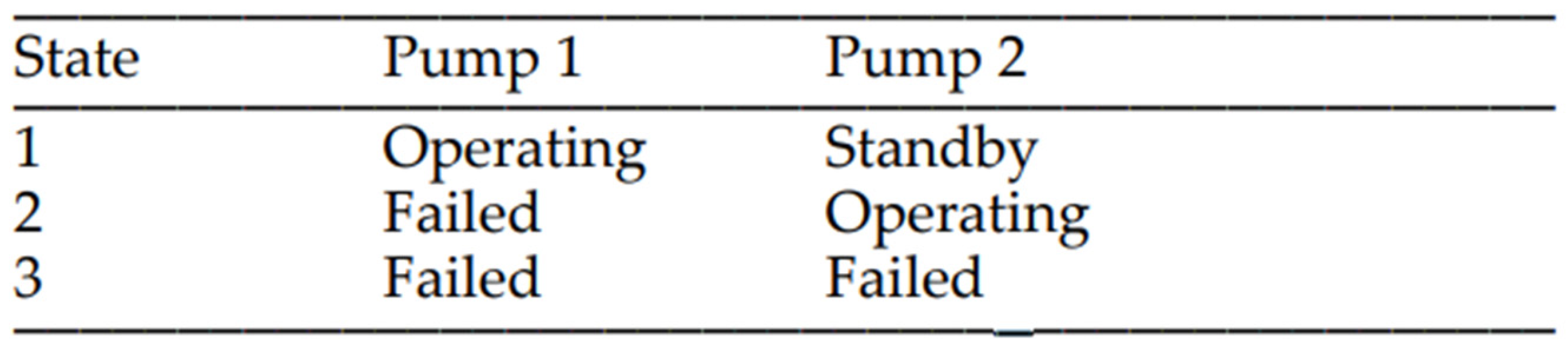
Using the Figure 1, it shows the different operating states, hence there is redundancy. As a main motor does not have any redundancy if it were to incur a major failure, we can only consider 3 states of operating, standby and failed. Referring to the DNV GL classifications under the systems and components of a ship section 2.1.5 it states that “The reliability and safety of components and complete units may also be documented by means of approved tests or service experience. The latter shall only be considered if a relevant load history can be documented”, (DNV GL, 2016).
Figure 1.
State of Oil Supply Pump (Anantharaman, Khan, Garaniya, & Lewarn, 2018).
This can be better interpreted by saying the comments should be logged and recorded. This can then be assessed to see any abnormalities within the recorded information. According to Charles Ebeling the Weibull distribution model is one of the most useful probability distributions within reliability. The distribution function can be used for both increasing and decreasing failure rates which makes it a common theoretical probability method alongside normal Lognormal and Gamma distributions. “These distributions have hazard rate functions that are not constant over time, thus providing a necessary alternative to the exponential failure law”, (Ebeling, 1997). The normal distribution is an alternative way to model fatigue wear out phenomena due to the relationship between the Lognormal distribution. This method allows the use of analysing further Lognormal probabilities as it provides a common bell shaped curved. The Gamma model has a similar distribution profile to Weibull as it has a family that includes the Exponential distribution.
According to research by Pinheiro and Bates, the log-likelihood of nonlinear mixed-effects models proves highly effective in handling unbalanced repeated-measures data in various fields, such as pharmacokinetics and economics (Pinherio & Bates, 2012). This methodology is also applicable when using distribution models for reliability assessments. As previously discussed, it can be applied to Weibull, Gamma, and Normal probability distributions, and the log-likelihood is particularly useful when applied to Probability Density Functions (PDFs).
The Mean Time to Failure (MTTF) is a critical metric in reliability analysis. As defined by Cadence, MTTF “evaluates the reliability of non-repairable items and equals the mean time expected until the first failure of a component, assembly, or system.” In essence, MTTF represents the predicted lifespan of a system or component. It is calculated by dividing the total hours of operation by the total number of units. This metric is widely used to predict when individual system components might fail, facilitating planned maintenance, repairs, or replacements to prevent unexpected breakdowns.
Charles Ebeling describes Fault Tree Analysis as a valuable tool for performing safety assessments on failures. According to Ebeling, “A fault tree analysis is a graphical design technique that provides an alternative to reliability block diagrams” (Ebeling, 1997). He outlines six key steps in conducting a Fault Tree Analysis:
- Define the system, its boundaries, and the top event—For example, the reliability of a vessel’s main propulsion engine.
- Evaluate the system using a data-driven model—Identify and characterize the combination of events leading to failures.
- Construct the fault tree—Graphically represent the total system and its events, typically focusing on failures of individual components.
- Perform a qualitative evaluation—Identify the combinations of events contributing to the top event, such as a failure in the main propulsion engine.
- Conduct a quantitative evaluation—Assign probabilities and reliability values to the events defined in the fault tree.
- Present findings and conclusions—Summarize the results of the analysis with respect to the reliability of the main propulsion engine and its subsystems.
This study seeks to develop a data-driven model and Fault Tree Analysis (FTA) to predict the reliability of the main engine onboard ships. The structure of this paper is outlined as follows: Section 2 details the Materials and Methods used in the research; Section 3 discusses the Results and Discussions; and Section 4 concludes the study with key findings and implications.
2. Materials and Methods
The methodology for this study is based on the data collected from on-board marine engineers. A combined approach utilizing three data-driven models is employed to extract and identify the parameters that define the characteristics of the dataset. The Fault Tree Analysis (FTA) serves as the reliability method, enabling the evaluation and analysis of the data-driven models to establish relationships between subsystems and derive the overall reliability of the system.
This integrated methodology aims to determine the total reliability of a vessel’s main propulsion engine, considering each subsystem’s contribution. Graphical plots of failure running hours are generated using Probability Density Functions (PDFs) and Cumulative Density Functions (CDFs), providing a visual representation of the data. These distributions help validate the consistency of results and ensure accurate analysis. The graphical representation also highlights the failure running hour data for each subsystem, offering a clear overview of performance metrics.
The data-driven models applied in this study include Gamma, Weibull, and Normal distributions, allowing for the inclusion of a wide range of failure probabilities. By integrating these models into the FTA, reliability functions are defined for each subsystem and used to calculate the total reliability of the vessel’s propulsion engine. This approach combines theoretical modelling with practical insights to achieve a comprehensive reliability assessment.
2.1. Data Driven Model
The failure running hour data is filtered through MATLAB, filtering any failure running hours presented as zero or below as the domain of time must be greater than zero hours. This can be represented by the following domain.
Therefore, using the fit functions the distributions can be assessed for the Weibull, Gamma, and the Normal functions for both the PDF and the CDF. This is represented in the example below with the left graph in Figure 2 suggesting the PDF and the right representing the CDF.
Figure 2.
Example of CDF and PDF.
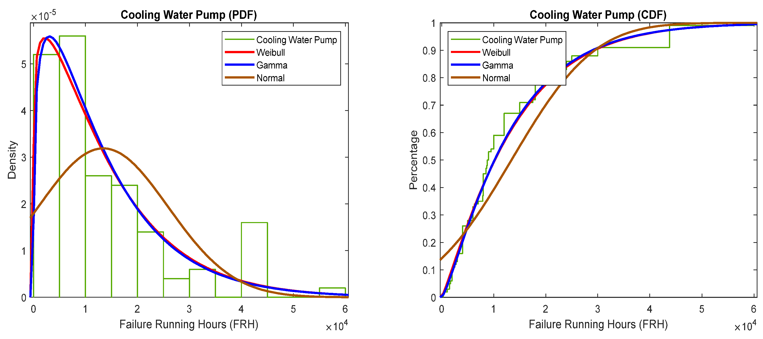
Figure 2 provides a visual representation of the density functions, showing that the Weibull and Gamma probability curves align with the distributions. However, the Normal distribution does not align, which will be supported by the higher log-likelihood value or the curve of best fit. MATLAB is used to calculate log-likelihood values, determining the best-fitting distribution based on the numerical value closest to 1.
The fitted data will yield corresponding values that establish relationship coefficients. These coefficients will be utilized to generate probabilities and reliability metrics. Key calculations will include metrics such as mean time to failure (MTTF), median, and standard deviation. The data will incorporate the following variables presented in Table 1 to ensure accurate analysis.
Using the distribution coefficients derived from all applied methods, mathematical formulas can be established based on the best-fitting models identified in MATLAB. These formulas represent the Probability Density Functions (PDFs) for analyzing reliability across the three selected models. The equations incorporate parameters optimized by MATLAB, ensuring accurate assessment of reliability. The PDF equations for each reliability model can be expressed as follows, where:
Weibull Probability Density Function with a domain of
(EQ. 1)
Gamma Probability Density Function with a domain of
(EQ. 2)
Normal Probability Density Function with a domain of
(EQ. 3)
Equations 1 to 3 represent the best-fit Probability Density Functions (PDFs) for the three selected distribution methods, determined by their respective highest log-likelihood values. These equations enable the calculation of the Mean Time to Failure (MTTF), providing an estimate of the average time to failure for each component based on the available data. The calculated MTTF values for all three methods will be used to evaluate the reliability of the main propulsion engine. Each subsystem’s reliability will contribute to the overall reliability of the main propulsion engine, ensuring that every component’s impact on the system is accounted for in the final analysis.
Weibull MTTF domain of
(EQ. 4)
Gamma MTTF domain of
(EQ. 5)
Normal MTTF domain of
(EQ. 6)
By utilizing the mean time to failure (MTTF) for each system and component, the reliability at a given elapsed time can be calculated and incorporated into the Fault Tree Analysis (FTA). This approach evaluates the overall reliability of the system at the expected failure time for all components.
The reliability equations can then be used to generate a total probability graph, visually representing the reliability of individual subsystems along with the overall reliability of the main engine. The FTA framework enables the construction of system reliability by logically combining the reliability of various subsystems through defined statements. The following equations represent the reliability functions for each selected probability distribution, providing the foundation for these analyses. Let me know if you’d like further assistance with refining or expanding on this content.
Weibull Reliability with respect to time
(EQ. 7)
Gamma Reliability with respect to time
(EQ. 8)
Normal Reliability with respect to time
(EQ. 9)
Equations 1 to 9 are sourced from the study ‘An Introduction to Reliability and Maintainability Engineering’, (Ebeling, 1997).
2.2. Fault Tree Analysis
Using Fault Tree Analysis (FTA), the main propulsion engine system is represented using a combination of symbols. This approach follows the four-step process outlined by Charles Ebeling: defining the system, constructing the fault tree, identifying key events, and assigning failure probabilities. The symbols commonly used in fault trees include two primary logical gates: the ‘AND’ and ‘OR’ gates, which describe how events occur within the system. The ‘AND’ gate represents a system primarily arranged in series, lacking redundancy, as all components must function for the system to operate. In contrast, the ‘OR’ gate represents a parallel system, implying a higher level of redundancy since only one component needs to function for the system to remain operational. These gates are used to relate to various event types, including resultant, basic, and incomplete events, which further extend to conditional and normal events. The relationships and impacts of these events can be effectively summarized in the following diagram.
| Shape | Event |
 |
AND gate. A logic gate which outputs only when all inputs have occurred () |
 |
OR gate. A logic gate which outputs if at least one input event has occurred () |
 |
Resultant event. A fault resulting for the logical combination of other fault events |
 |
Basic event. An independent elementary event representing a basic fault or component. |
 |
Incomplete event. An event that has not been fully developed due to lack of knowledge. |
 |
Transfer-in and Transfer-out. Used to link sections that are not contiguous or appear on separate pages. |
 |
Conditional event. A condition or restriction connected to a logical gate |
 |
Normal event. A normally occurring event that is not a fault |
Normal event. A normally occurring event that is not a fault
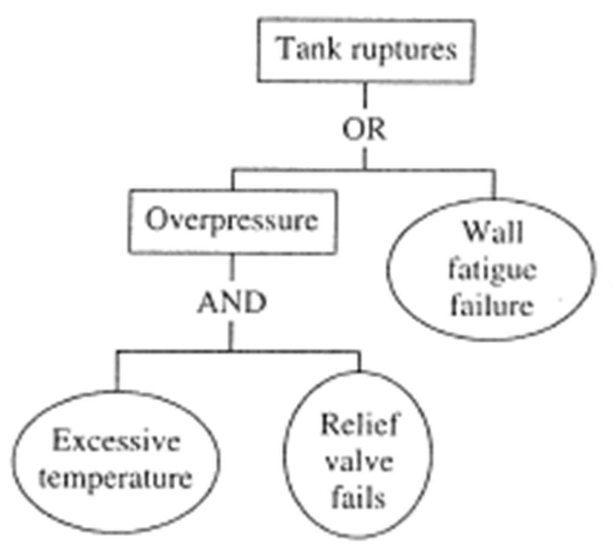
An example of the Fault Tree Analysis can be represented by the following figure with both the ‘and’ and ‘or’ gates.
Figure 3 illustrates the application of logical gates in Fault Tree Analysis. It demonstrates that both excessive temperature and relief valve failures must occur for the operation to proceed through the ‘AND’ gate. If either event fails, the resultant condition will be overpressure within the tank, which then leads to an ‘OR’ gate. At this gate, only one failure—either overpressure or wall fatigue—needs to occur for the resulting event, a tank rupture, to take place.
Figure 3.
Example of a fault tree (AND + OR gates), (Ebeling, 1997).
By incorporating Boolean functions alongside the reliability equations for each subsystem, the overall reliability of the vessel’s main propulsion engine can be determined. This analysis enables the calculation of the engine’s reliability over time, considering the interconnections and failure probabilities of its subsystems.
3. Results and Discussion
Using the collected data accumulated, a previous survey of the FRH obtained for all 26 systems and 101 different respondents. The data was obtained from the published article which conducted a survey from onboard marine engineers. The systems recorded can be shown in the figure below with the main propulsion engine leading into four sub systems Lube Oil, Cooling System, Scavenge System, and Fuel Oil.
3.1. Distribution Methods
Figure 4 illustrates all the systems analyzed and incorporated into the Fault Tree Analysis (FTA). The data, filtered and processed through MATLAB’s distribution filter, enables the creation of Probability Density Functions (PDFs) and Cumulative Density Functions (CDFs). These distributions are visually examined to identify correlations within the results.
Figure 4.
Sub Systems of the recorded data set.
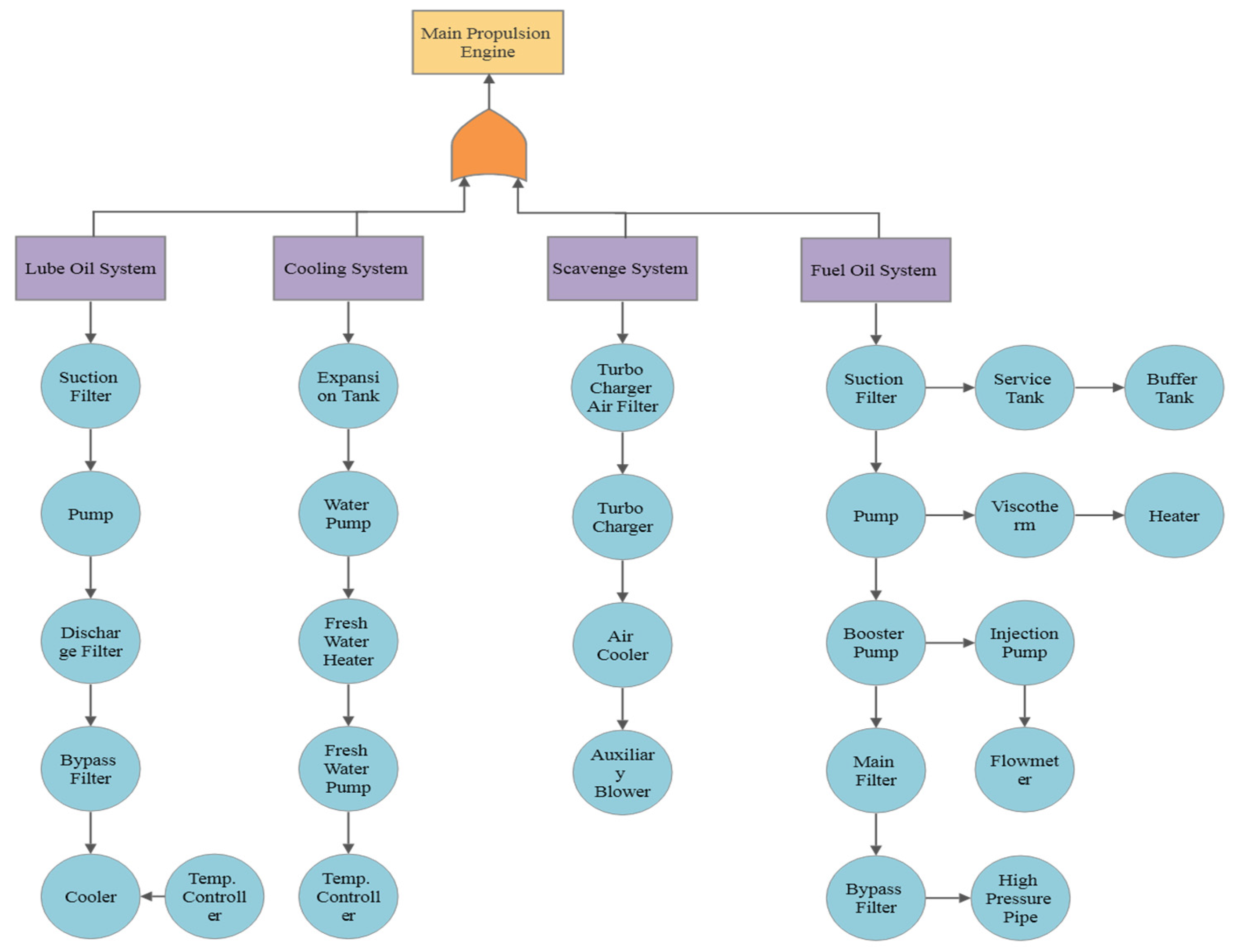
Figure 5 provides a comparison of three distributions—Weibull, Gamma, and Normal—modelled at a 95% confidence level. The Weibull and Gamma distributions initially appear to align more closely with the dataset trends compared to the Normal distribution. This observation is supported by the log-likelihood function, which generates numerical values to determine the best-fit function. Based on the values obtained, Figure 5 suggests that the Gamma distribution provides the most accurate fit, further strengthening its reliability in modelling the data.
Figure 5.
Lube Oil Temperature Controller (PDF and CDF).
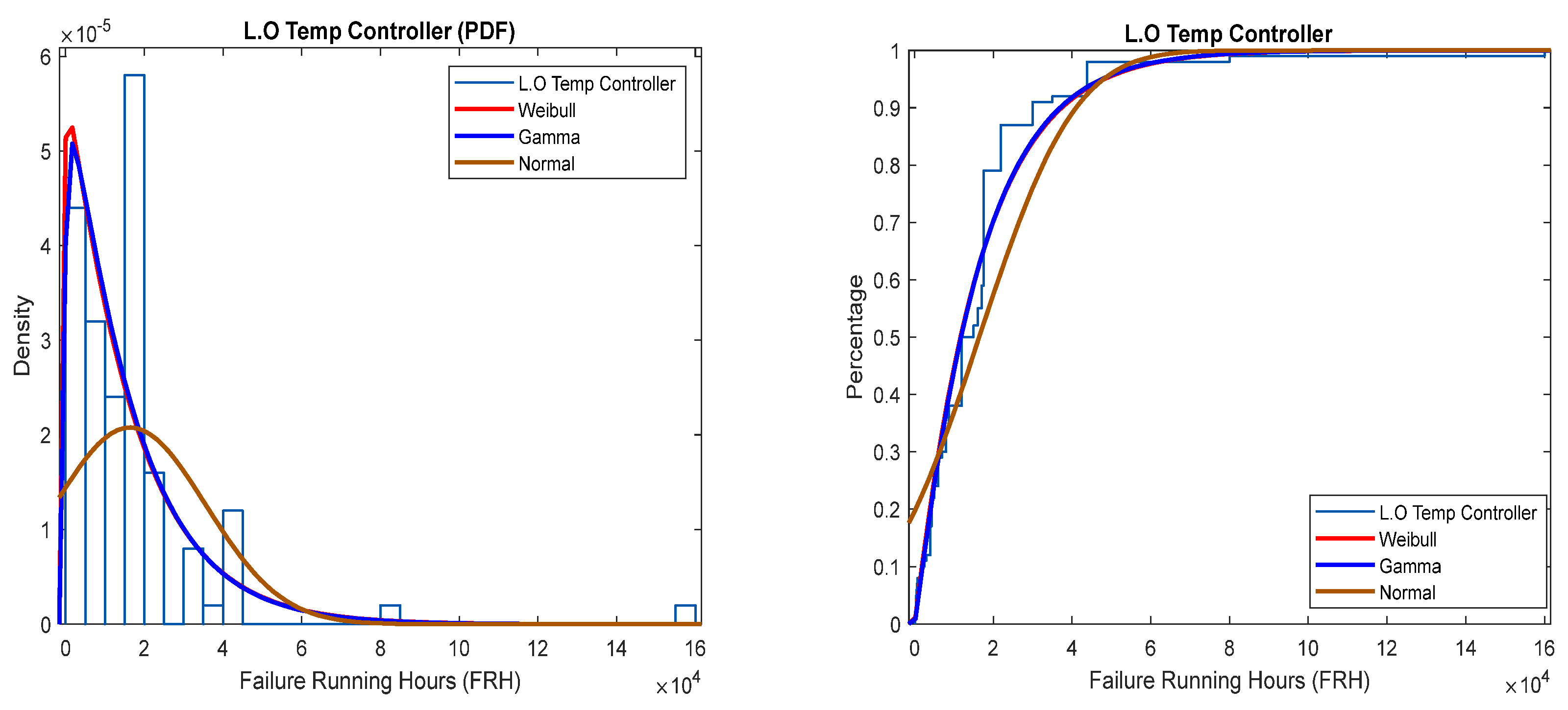
Error! Reference source not found. shows that the Gamma distribution has a log likelihood that is 0.17 greater than the Weibull function. This suggests the best fit distribution to be the Gamma function.
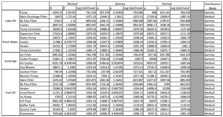
The variables derived from the graphs, including shape parameters, scale parameters, and characteristic life, are summarized in Table 1. Table 7, located in Appendix A—Distribution Selection, presents all the distribution values associated with the reliability equations, mean time to failure (MTTF), and density functions. These results are consolidated into the following tables, where the selection of the distribution is based on the highest log-likelihood values.
Table 3, Table 4, Table 5 and Table 6 outline the distribution results for all 26 systems, with the Gamma distribution emerging as the most commonly observed. Notably, Table 6 reveals a trend within the Weibull distribution, as 6 out of the 11 subsystems align with it. Using the data presented in Table 7, the reliability of each system can be calculated and incorporated into the Fault Tree Analysis (FTA).
The calculation of variables follows a standardized process, exemplified here using the Lube Oil Temperature Controller with the Gamma distribution. This approach ensures consistency and accuracy in determining reliability values for each subsystem.
(EQ.8)
Using Error! Reference source not found. with Alpha = 14986.8 and gamma = 1.096
This is calculated using the MATLAB command gamcdf which is used by the following
Similar can be calculated using Weibull reliability equation using the Lube Oil Main Discharge Filter. This can be shown by the following equations.
(EQ. 7)
Using Error! Reference source not found. with Theta = 18475 and Beta = 1.271
For both reliability functions, this can be used over a range of time to assess the reliability of each component which will be used within the Fault Tree Analysis.
3.2. Fault Tree Analysis
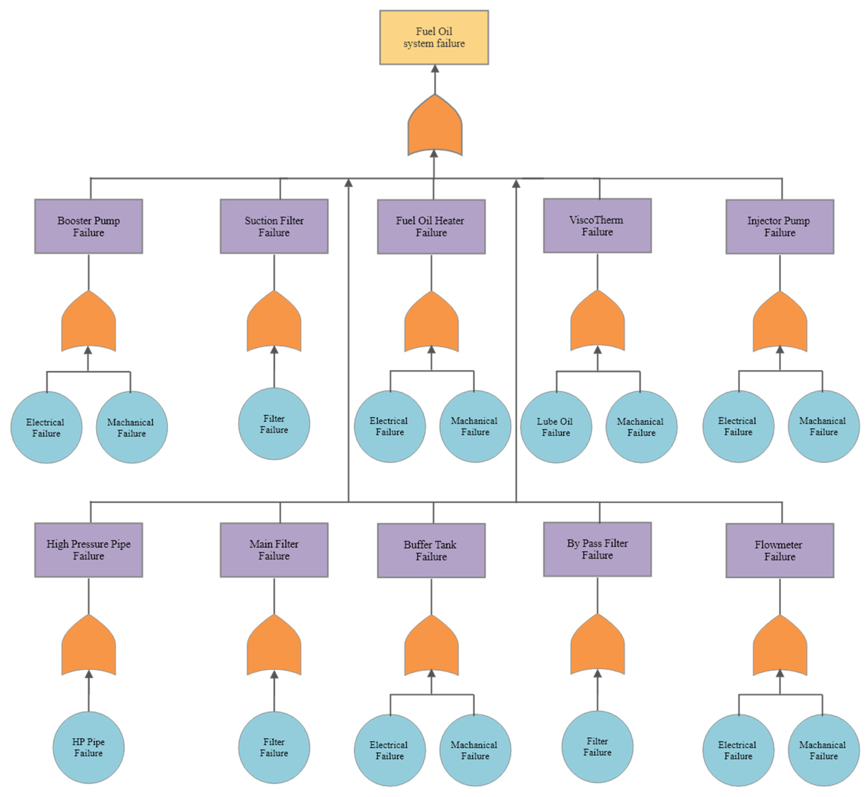
The Fault Tree Analysis (FTA), as previously discussed, is a reliability method that provides a simplified representation of the entire system using “AND” and “OR” gates to facilitate conditional analysis. The system can be divided into two levels: the primary system, which is the main propulsion engine, and the secondary level, comprising its four primary subsystems. These subsystems—Lube Oil, Cooling System, Scavenge System, and Fuel Oil—are configured to pass through an “OR” gate. This configuration is visually represented in the Figure 6.
Figure 6.
Main Propulsion Engine System Fault Tree Analysis.
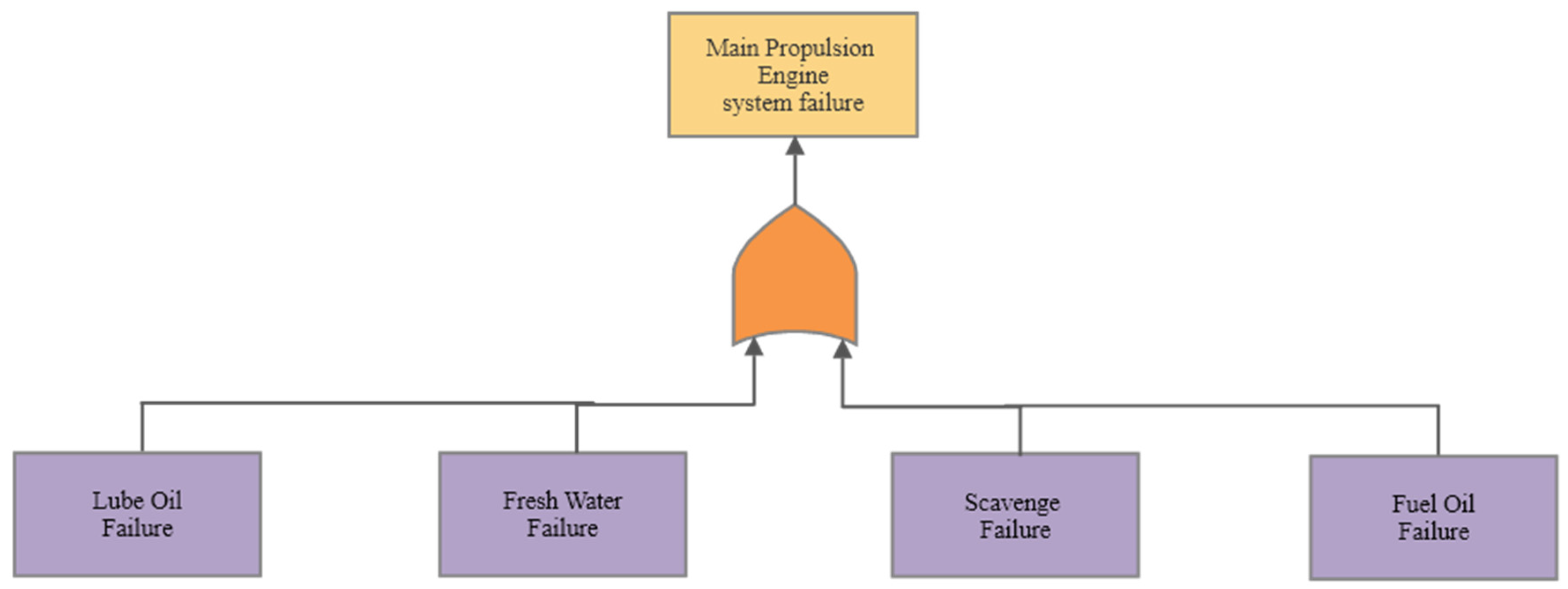
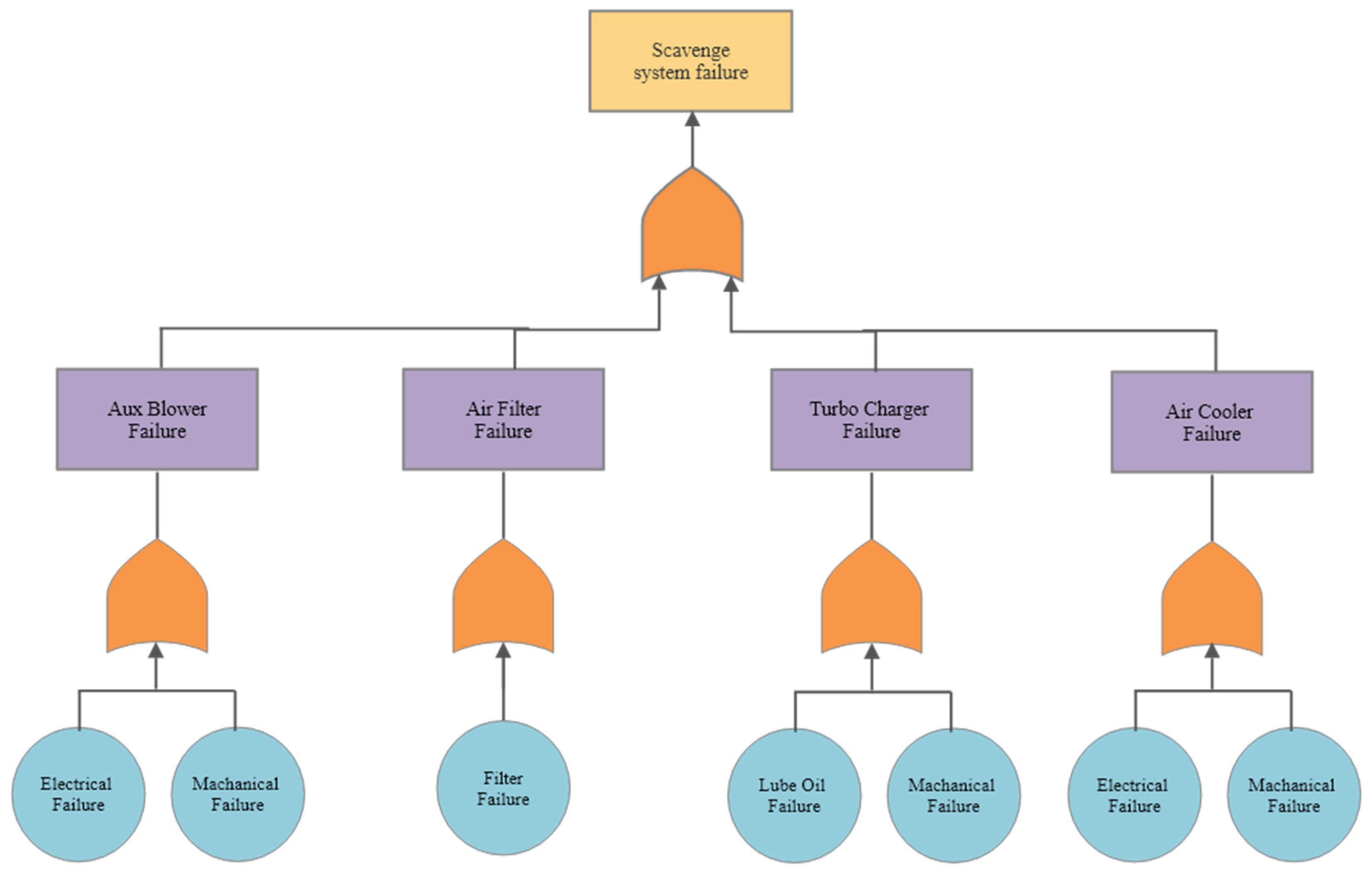
Error! Reference source not found. shows the Fault Tree Analysis of the main propulsion engine which connects using an “or” gate, this suggests no redundancy systems for the calculations. This indicates it is a series systems as all four systems must be operational for the propulsion of a ship to occur. Alternatively, if one system fails no propulsion will be applied as the engine is inoperable. This same concept can be applied to each system which can be shown in Error! Reference source not found. and Appendix B: Fault Tree Analysis. This shows a similar approach, although the event that fails allows for conditional failures which is shown as the electrical/mechanical failure. The scavenge system fault tree shows that all systems will need to be operative for the outcome of the system to function.
Figure 7.
Scavenge System Fault Tree Analysis.
The above or gates can be used to define the events using Boolean algebra which is used to express in terms of nonredundant systems. From the figure above, the nonredundant systems can be shown by the following equation.
(EQ.10)
Using the reliability results for the scavenge system equation 10 is restructured using the reliability equation. This is shown by the following.
Using the equation above, the reliability distributions can be calculated for time as failure running hours for all four systems. The following figures show the decrease in reliability as time increases.
The Figure 8 and Figure 9 above all show similar correlation with differing failure running characteristics as Weibull and Gamma typically have similar styles. Using Error! Reference source not found. the total reliability of the system can be determined using the same process however only using the outcomes of the sub systems from Figure 8 and Figure 9.
Error! Reference source not found.The outcome will represent the total system reliability using both the Weibull and Gamma distributions using the Fault Tree Analysis process. Thus, the following figure will represent the total reliability as shown below.
Error! Reference source not found. shows the reliability of the total system which is the vessels main propulsion engine. This shows the reliability of the main propulsion engine between time zero and a reliability of zero at approximately 900 failure running hours. The data for all 26 systems was used to develop the final Fault Tree Analysis which is based on the Weibull and Gamma models with the values of theta, alpha, beta, gamma. This was estimated using MATLAB at the 95% confidence level which produced the reliability against the failure running hours. This data can only be taken as an estimation as no censoring is available within the data set. “Censored data is any data for which we do not know the exact event time”, (Reid, 2021). With the three types of censoring which are right censored, left censored, and interval censored. Using the censored data, the failures can be recorded as accurate or not accurate. The most common for this data set would be the interval censored data suggesting for items such as filters may fail before the failure running data is recorded.
Using the fault tree analysis within the vessels main propulsion engine it shows that all systems are considered important to the engine and are considered equal as any system failure will result in engine failure. However, each system will have a different repair rate suggesting a failure of the filter may have a different impact when compared to a pump failure. Using this assumption, the failure within a repair analysis will be considered different.
4. Conclusions
This study demonstrates how Fault Tree Analysis (FTA) provides a time-based reliability overview of a vessel’s main propulsion engine, utilizing data collected from surveys. The FTA highlights the relationships and conditions of each subsystem in relation to the main engine, using correlations and distributions across all 26 systems to consolidate them into four key subsystems: Lube Oil, Freshwater, Scavenge, and Fuel Oil. These subsystems were analyzed to calculate reliability metrics over time for each.
The findings indicate the overall reliability of the main propulsion engine, offering critical insights for scheduling maintenance overhauls and identifying key operational thresholds within the marine industry. By subdividing the main propulsion engine into four distinct subsystems, the reliability outcomes provide a clearer understanding of failure probabilities at various elapsed times or failure running hours.
This study contributes to the marine industry by enhancing the reliability analysis of shipping operations, supporting the optimization of maintenance schedules and informing future design improvements. These results pave the way for advancing operational safety and efficiency in maritime transportation systems.
Acknowledgments
The authors extend their heartfelt gratitude to the marine engineers who generously contributed their time and expertise to the data collection process for this research. Your invaluable support and participation were instrumental in the success of this study.
Appendix A: Distribution Selection

Table A1.
Distribution Selection table with log likelihood.
 |
Appendix B: Fault Tree Analysis
Figure A1.
Lube Oil System Fault Tree Analysis.
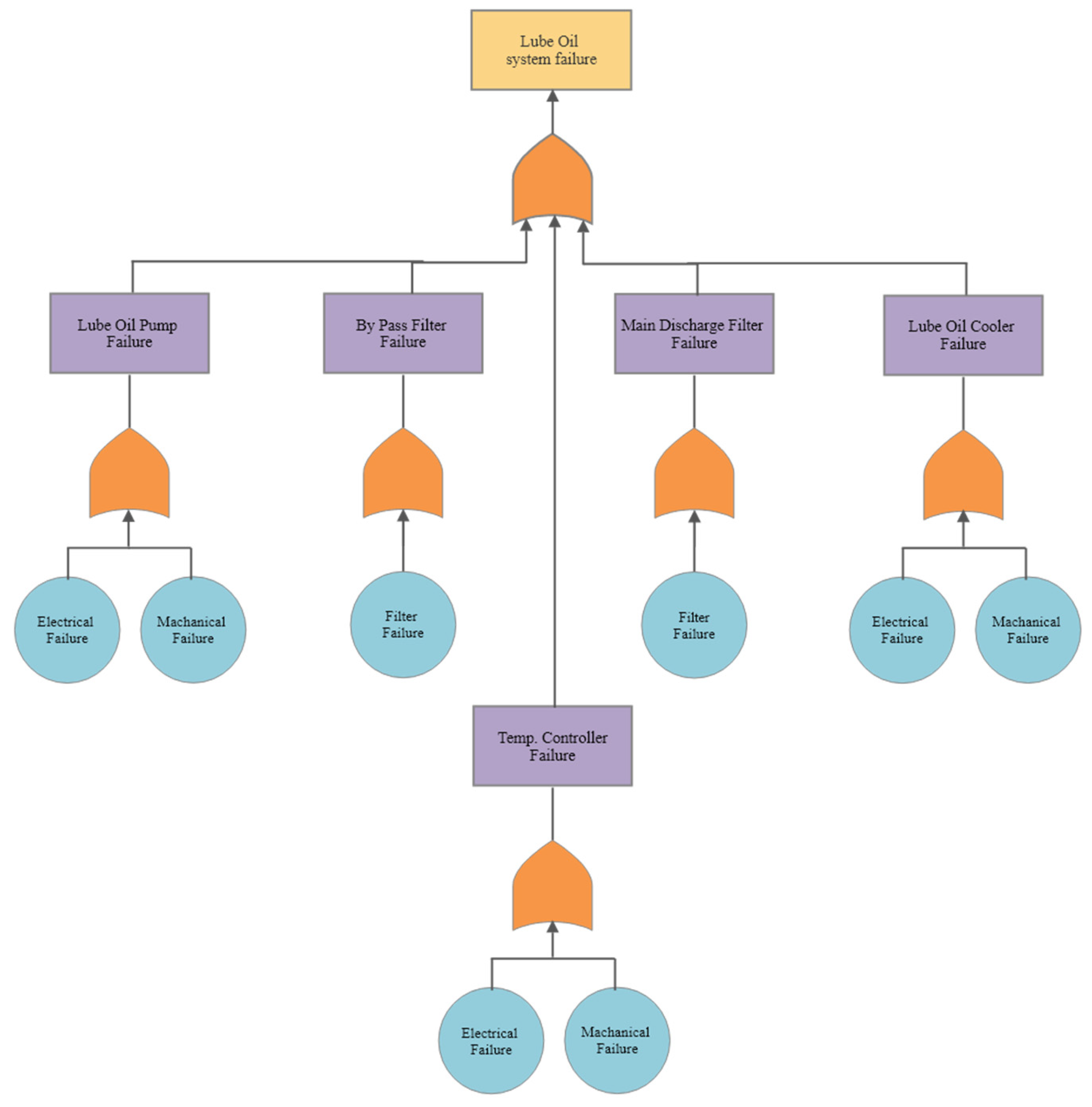
Figure A2.
Fresh Water System Fault Tree Analysis.
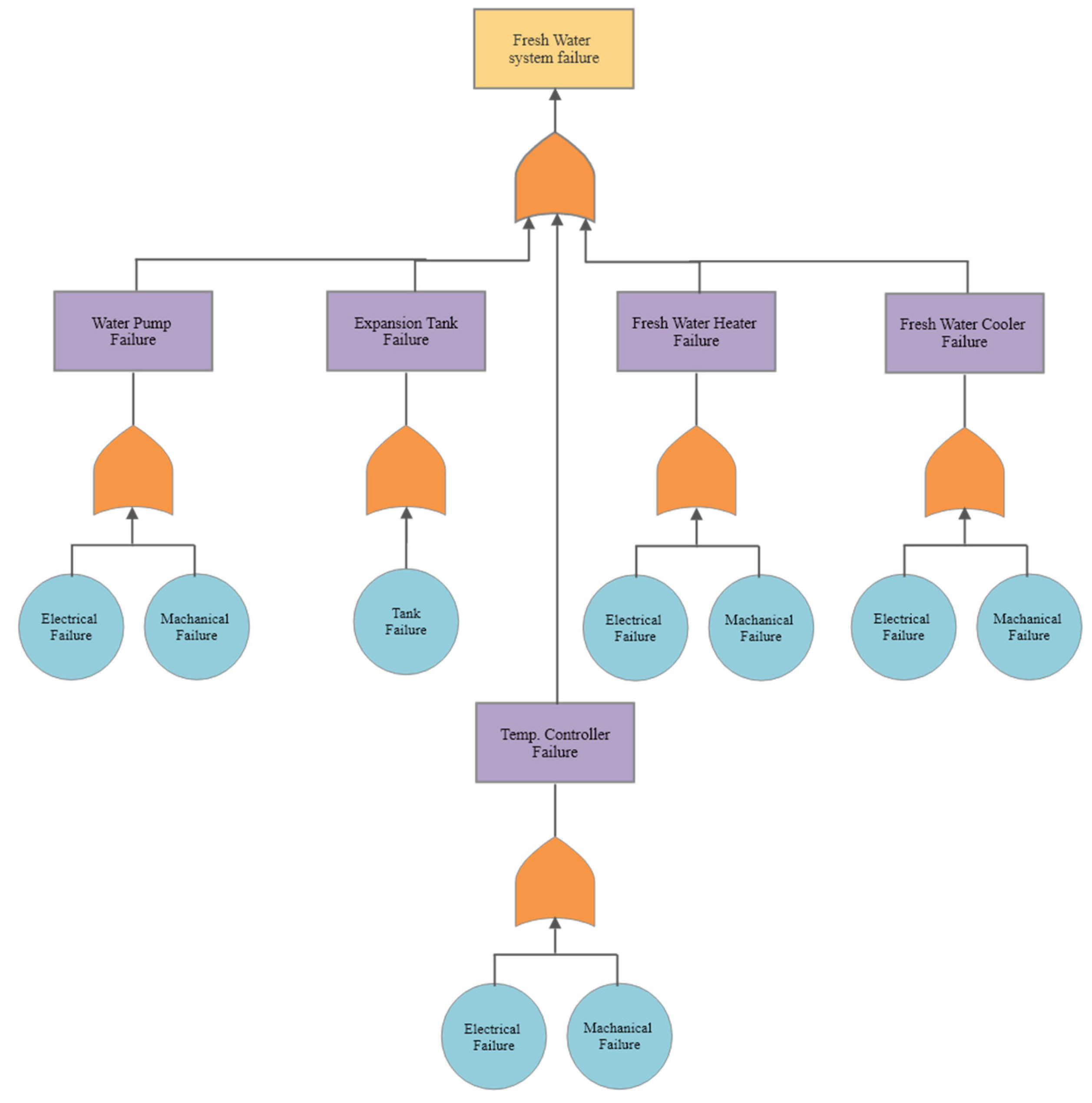
Figure A3.
Fuel Oil System Fault Tree Analysis.
References
- Anantharaman, M., Islam , R., & Garaniya, V. (2018). Reliability Assessment of Main Engine Subsystems Considering Turbocharger Failure as a Case Study. TransNav, the International Journal on Marine Navigation and Safety of Sea Transportation, 271-276. [CrossRef]
- Anantharaman, M., Islam, R., Khan, F., Garaniya, V., & Lewarn, B. (2019). Data Analysis to Evaluate Reliability of a Main Engine. Australia, Canada: TransNav. [CrossRef]
- Cadence PCB Solutions. (2021). MTBF, MTTR, MTTF, and FIT: Design Reliability Measures for Electronics. Retrieved from Cadence: https://resources.pcb.cadence.com/blog/2020-mtbf-mttr-mttf-and-fit-design-reliability-measures-for-electronics.
- Cagnassola , M. E. (2021, 5 28). Maritime Traffic Halted in Bosphorus Strait After Massive Oil Tanker Narrowly Averts Disaster. Retrieved from Newsweek: https://www.newsweek.com/maritime-traffic-halted-bosphorus-strait-after-massive-oil-tanker-narrowly-averts-disaster-1596066.
- Castonguay, J. (2020). Internatinal Shipping: Globalization In Crisis. North Salem: Richard Falco: Vision Project Inc.
- DNV GL. (2016). Part 4 Systems and components Chapter 2 Rotating machinery, general. DNV GL.
- Ebeling, C. (1997). An Introduction to Reliability and Maintainability Engineering. United States of America: McGraw-Hill.
- Mohammed, A. Z. (2021). Suez Canal Authority swiftly repairs container ship after sudden engine failure. Middle East : ARAB NEWS.
- Molland, A., Turnock, S., & Hudson, D. (2011). Ship Resistance and Propulsion. Cambridge: Cambridge University Press.
- Pinherio, J. C., & Bates, D. M. (2012, February 21). Approximations to the Log-Likelihood Function in the Nonlinear Mixed-Effects Model. Retrieved from Taylor & Francis Group. [CrossRef]
- Regattieri, A., Manzini, R., & Battini, D. (October 2010). Estimating reliability characteristics in the presence of censored data: A case study in a light commercial vehicle manufacturing system. America: Science Direct. [CrossRef]
- Reid, M. (2021, June 1). What is censored data. Retrieved from Reliability : https://reliability.readthedocs.io/en/latest/What%20is%20censored%20data.html.
- Winterbone, D., Yates, D., Clough, E., Rao, K. K., Gomes, P., & Sun, J.-H. (1994). Combustion in High-Speed Direct Injection Diesel Engines—A Comprehensive Study. US: Sage Journals. [CrossRef]
- Xiros, N. (2002). Introduction. In Robust Control of Diesel Ship Propulsion (pp. 1-11). London: Springer London.
- Zhang, S., Chenhui, R., Liyong, W., Xiaojian, Y., & Haiping, D. (2018). Reliability Analysis of Aero-Engine Main Fuel System Based on GO Methodology. Germany: Shanghai Jiao Tong University and Springer-Verlag GmbH Germany.
Figure 8.
Lube Oil and Fresh Water Reliability Analysis.
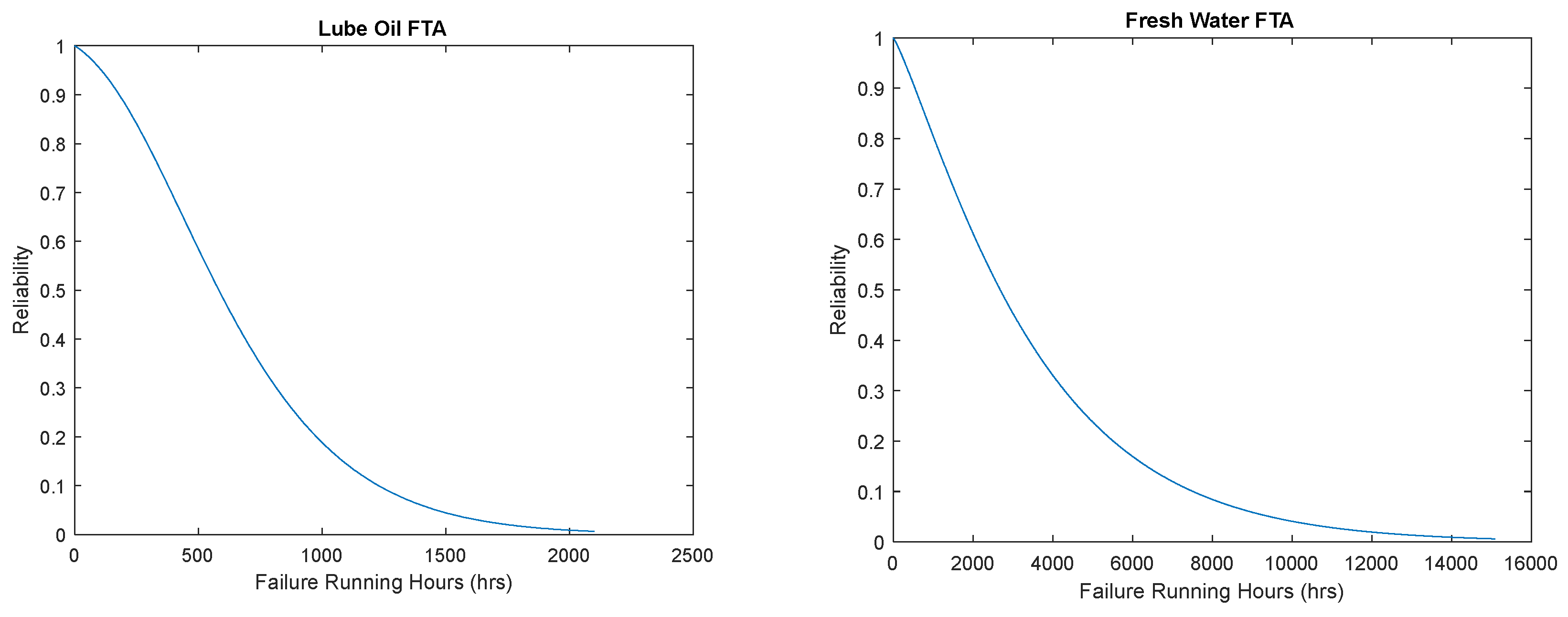
Figure 9.
Scavenge and Fuel Oil Reliability Analysis.
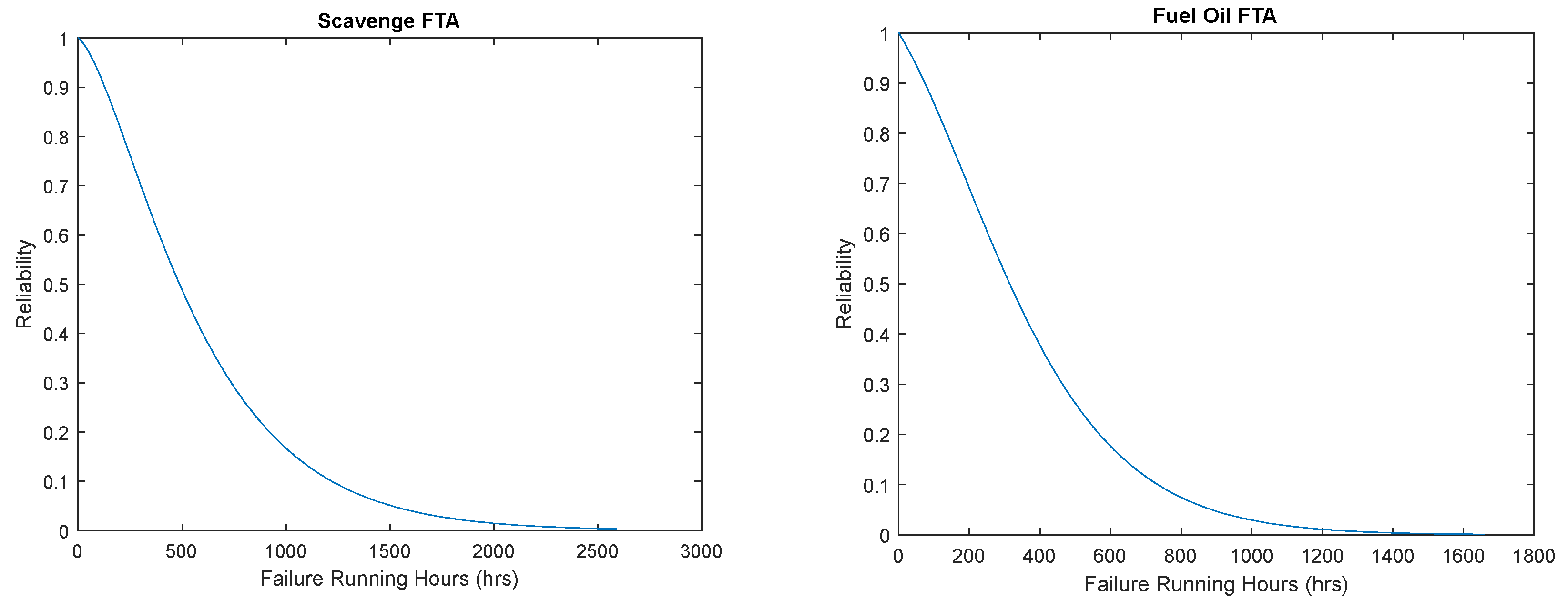
Figure 10.
Main Propulsion Engine Reliability Analysis.
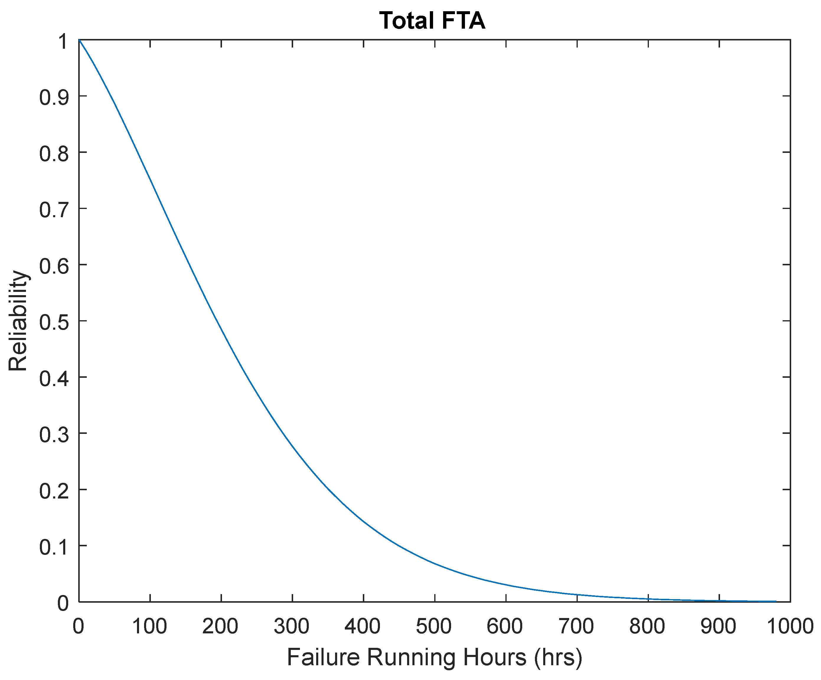
Table 1.
Distribution Methods.
| Distribution Methods | ||
| Weibull | ϴ—Characteristic Life | β—Shape Parameter |
| Gamma | α—Scale Parameter | γ—Shape Parameter |
| Normal | µ—Mean | σ—Standard Deviation |
Table 2.
Distribution Selection for Lube Oil Temperature Controller.
| Distribution Type | Log Likelihood |
| Weibull | -1070.53 |
| Gamma | -1070.36 |
| Normal | -1127.66 |
Table 3.
Distribution Fits Lube Oil Systems.
| Lube Oil | ||||
| Pump | Main Discharge Filter | Bypass Filter | Cooler | Temp Controller |
| Gamma | Weibull | Gamma | Gamma | Gamma |
Table 4.
Distribution Fits Fresh Water Systems.
| Fresh Water | ||||
| Expansion Tank | Water Pump | Cooler | Heater | Temp Controller |
| Gamma | Gamma | Gamma | Gamma | Weibull |
Table 5.
Distribution Fits Scavenge Systems.
| Scavenge | |||
| Air Filter | Turbo Charger | Air Cooler | Aux Blower |
| Gamma | Gamma | Weibull | Gamma |
Table 6.
Distribution Fits Fuel Oil Systems.
| Fuel Oil | |||||
| Suction Filter | Booster Pump | Main Filter | Bypass Filter | Heater | ViscoTherm |
| Gamma | Gamma | Gamma | Gamma | Weibull | Weibull |
| Injector Pump | H.P Pipe | Buffer Tank | Service Tank | Flowmeter | |
| Gamma | Weibull | Weibull | Weibull | Weibull | |
Disclaimer/Publisher’s Note: The statements, opinions and data contained in all publications are solely those of the individual author(s) and contributor(s) and not of MDPI and/or the editor(s). MDPI and/or the editor(s) disclaim responsibility for any injury to people or property resulting from any ideas, methods, instructions or products referred to in the content. |
© 2025 by the authors. Licensee MDPI, Basel, Switzerland. This article is an open access article distributed under the terms and conditions of the Creative Commons Attribution (CC BY) license (https://creativecommons.org/licenses/by/4.0/).
Copyright: This open access article is published under a Creative Commons CC BY 4.0 license, which permit the free download, distribution, and reuse, provided that the author and preprint are cited in any reuse.


