Submitted:
02 April 2025
Posted:
04 April 2025
You are already at the latest version
Abstract
Cation exchange capacity (CEC) is an important trait related to soil fertility and nutrient retention used for breeding in agricultural forage crops. However, its genetic background in oat (Avena sativa L.) remains poorly understood. In this study, four genome-wide association study (GWAS) models—Mixed Linear Model (MLM), FarmCPU, BLINK, and BayesCπ—were considered to identify SNPs associated with CEC based on publicly available genotypic and phenotypic data. Principal component analysis (PCA) was performed to account for population structure, and the models were compared in terms of the number of significant SNPs, their overlap, and visualizations (Manhattan and QQ plots). The results showed that FarmCPU provided the highest detection power, MLM the highest stringency, BLINK demonstrated the highest analysis speed, and BayesCπ allowed to accurately estimate SNP effects and explained variance. The obtained results provide a comparative view of the performance of GWAS models in studying complex agronomic traits and confirm the need to select the method for specific breeding tasks of oats and other agricultural plants in general.
Keywords:
GWAS
; cation exchange capacity
; oat
; SNP
; FarmCPU
; BayesCπ
; MLM
; BLINK
Summary
Genome-wide association studies play a key role in the selection of agricultural feed crops across many parameters, including nutrient uptake and stress resistance. The cation exchange capacity (CEC) is an important indicator for soil fertility and nutrient uptake, but its genetic nature in the oat (Avena sativa L.) studied in this paper is currently poorly understood. Open phenotypic and genotypic oat data were used in the study, and four GWAS models (MLM, FarmCPU, BLINK, and BayesCπ) were applied to evaluate their effectiveness in detecting SNP associated with CEC. When evaluating the results, it can be stated that in this work FarmCPU showed the highest sensitivity, MLM - better control of false finds, BLINK - high analysis speed, and BayesCπ gave accurate evaluations of SNP effects. These results can help with the selection of the GWAS model depending on the research goals and resources for subsequent work.
Introduction
Oats (Avena sativa L.) are an important cereal crop that plays a significant role in the production of feed and food due to their high nutritional value, resistance to adverse conditions, and ability to improve soil structure [1]. In the current conditions of climate change and resource depletion, the selection of oats with improved agronomic characteristics is of particular importance. One of these characteristics is stress resistance and increased absorption of nutrients from the soil [2,3].
One of the key traits associated with plant fertility and the efficiency of element absorption from the soil is the cation exchange capacity (CEC) - a measure of the ability to retain ionic nutrients in the rhizosphere [4]. A high CEC value promotes better absorption of macro- and microelements, such as potassium, calcium, and magnesium, and can be considered a promising indicator for the selection of more productive oat varieties [5,6].
CEC reflects the ability of the plant and the surrounding soil environment to retain cations, and thereby maintain stable and balanced plant nutrition. This is especially important under stressful conditions (e.g., drought, soil acidity), where the availability of nutrients can decrease drastically. Plants with high CEC retain elements in the rhizosphere more efficiently, reduce their leaching, and improve interactions with the microbiota involved in the mobilization of phosphorus and nitrogen [5,6]. In addition, CEC is associated with the morphology of the ion-transport systems of roots, as well as with the general adaptive capacity of the crop to poor soils and extreme conditions [7,8]. Despite such importance, CEC is rarely studied as a target trait in breeding, including due to the complexity of phenotyping and the lack of genetic studies [9]. Given the multifactorial nature of CEC and its dependence on complex genetic interactions, genome-wide association analysis (GWAS) methods are a powerful tool for identifying markers associated with this trait [10]. In recent years, GWAS has been widely applied to various traits in oats, from yield to disease resistance, but research on traits related to ion exchange and interactions with the soil environment remains limited [11,12]. There are many GWAS methods, differing in their approaches to accounting for population structure, power, and resistance to false positives. In this paper, four methods were compared: Mixed Linear Model, FarmCPU, BLINK, and BayesCπ. MLM (Mixed Linear Model) is a classic model that takes into account both genetic relatedness and population structure [13]. FarmCPU is an improved method that combines fixed and random effects to increase the power of the analysis [14]. BLINK is a method that is designed for rapid analysis and increased accuracy by excluding irrelevant markers [15]. BayesCπ is an approach based on Bayesian regression that provides accurate identification of markers with a strong effect [16].
Despite significant progress in the development of GWAS models, questions about which methods are most effective in analyzing CEC-like traits in the context of crop plants remain unanswered. This study aims to compare statistical power and robustness to false positives between methods, assess the impact of accounting for population structure, and identify optimal approaches for further use of GWAS in oat breeding programs.
Methods
A publicly available oat (Avena sativa L.) dataset provided by the Global Landrace Collection Project was used for the analysis. Genotypic and phenotypic data were downloaded from the Agricultural Research Service repository. This dataset is linked to the study by Maughan et al. (2019) published in Nature Communications [17].
The genotypic data is in VCF format and contains ~394,000 SNP markers after basic filtering. The phenotype was the cation exchange capacity (CEC) extracted from the soil trait table. This continuous trait reflects the ability of a plant to interact with the mineral part of the soil and assimilate cations.
To control population stratification, principal component analysis (PCA) was performed on the genotypic data. The first two principal components (PC1 and PC2) were included in the GAPIT models as covariates. This allows us to correct the influence of population structure and reduce the probability of false positive associations.
Four methods of association analysis were tested and compared: MLM, FarmCPU, BLINK, and BayesCπ. For the GAPIT models, a common set of SNPs and a single number of PCs (2) were used. In the case of BayesCπ, due to the high computational load, the analysis was performed on a subset of SNPs, while the following filters were observed: minimum minor allele frequency (MAF) ≥ 0.05; exclusion of SNPs with missing values.
Comparison of the efficiency of the models was carried out by the number of significant SNPs, the overlap of the top 100 SNPs between the methods, visualization of the results using Manhattan and QQ plots, and for BayesCπ, histograms of SNP effects and plots of the relationship between the effect, MAF and the proportion of explained phenotypic variance were additionally constructed. The analysis was performed in R 4.x using the following packages: GAPIT v3 for MLM, FarmCPU, and BLINK models; BGLR for BayesCπ analysis; ggplot2, VennDiagram, prcomp() and other standard visualization tools.
Results
A comparison of the number of significant SNPs showed different sensitivity of each of the methods. FarmCPU identified the largest number of significant markers (11), MLM — 7, BLINK — 4. The BayesCπ method, applied to a subset of SNPs, also identified 10 significant positions. These results reflect differences in approaches to controlling type I errors and model sensitivity. Manhattan plots (Figure 1, Figure 2 and Figure 3) show that FarmCPU identified clear peaks, including those with p-values above -log10(p) > 13, BLINK showed single high signals, but in smaller numbers, MLM gave a more uniform distribution of signals, without sharp spikes.
False positive results and False discovery rate were assessed based on the degree of overlap of the top 100 SNPs between three methods. To estimate possible false positives, a Venn diagram of the top 100 SNPs of each method was constructed (Figure 4). The overlap between the methods is extremely limited. MLM and FarmCPU do not share any SNPs, MLM and BLINK share 3 SNPs, FarmCPU and BLINK share 6 SNPs. All three methods together identified only 6 SNPs.
The QQ plot analysis allows us to assess the conformity of the p-value distribution with the expected one in the absence of associations, and thus to judge the presence of signals and possible inflation of Type I errors. FarmCPU (Figure 5a) shows a noticeable deviation from the diagonal in the right part of the plot, which indicates the presence of strong signals and increased sensitivity of the method. Despite the small inflation, the deviation starts quite late, which indicates an acceptable level of false positives. BLINK (Figure 5b) also shows a pronounced deviation from the null hypothesis in the tail of the distribution, but less extensive than that of FarmCPU. This indicates the presence of significant associations, but the number of strong signals is smaller, which is consistent with the number of detected SNPs. MLM (Figure 5c) gives a distribution close to the expected one, with a minimal deviation from the diagonal. This indicates high stringency of the model and a low level of inflation, but may also indicate a loss of sensitivity to weak and moderate effects.
For a more detailed analysis of significant SNPs identified by the FarmCPU method, plots of the minor allele frequency (MAF) were constructed (Figure 6a–c). Most of the highly significant and large-effect SNPs had low MAF, which is typical for rare variants with potential functional significance. One of the SNPs explained up to 8% of the phenotypic variance, indicating its possible role in the control of CEC.
The BayesCπ method allowed us to identify the most informative markers potentially involved in the formation of the CEC trait. 10 SNPs with the highest contribution were identified, for which the effects and the proportion of explained phenotypic variance were calculated (Table 1). The SNP effects ranged from 0.0029 to 0.0032, indicating a moderate influence of each individual locus. At the same time, each of these markers explained from 10.9% to 12.3% of the phenotypic variance, which can be considered highly informative for a complex agronomic factor.
To account for the population structure, Principal Component Analysis was performed. The scree plot (Figure 7) shows that the first two components explain most of the genetic variance (~23% and ~8%, respectively). Based on the results, 2 PCs were included in the model as covariates.
A limitation in this work was the use of BayesCπ only on a subset of SNPs due to the method’s high computational load. Because of this, the analysis was not performed on the entire SNP set (~394K), but only on a limited subset. This does not allow for a direct, full comparison with other methods on the entire dataset. In addition, the analysis was performed only for one trait (CEC), without testing the results on other phenotypes or samples. In the future, it will be possible to test the models on other traits and populations.
Conclusions
In this study, four GWAS methods were compared to identify SNPs associated with cation exchange capacity (CEC) in oats (Avena sativa L.).
The results confirm that the choice of method significantly affects the number, reliability, and interpretability of the associations found. FarmCPU and BayesCπ showed high sensitivity, while MLM provided strict control of false positive results. BLINK, in turn, showed exceptional speed in obtaining results.
The results of this work will help researchers select suitable GWAS models for the analysis of complex traits and contribute to the development of strategies for selecting optimal GWAS models for the analysis of agronomically significant traits.
References
- Tang, Y. et al. (2021). Genomic prediction in oat breeding. Plant Genome, 14(3).
- Redaelli, R. et al. (2013). Grain yield and quality in Italian oats. Euphytica, 190(2).
- Bekele, W. A. et al. (2018). Genome-wide association study of agronomic traits in oat. Plant Genome, 11(2).
- Brady, N. C., & Weil, R. R. (2008). The Nature and Properties of Soils. Pearson.
- Hu, Y. et al. (2021). Cation exchange capacity as a trait in plant nutrition. Journal of Soil Science and Plant Nutrition, 21(1).
- Yakovlev, I. A. et al. (2022). Genetics of soil-plant interactions. Frontiers in Plant Science, 13.
- Hinsinger, P. et al. (2009). Rhizosphere: a new frontier for soil biogeochemistry. Journal of Geochemical Exploration, 100(2).
- Ryan, P. R. et al. (2001). Function and regulation of root ion channels. Physiologia Plantarum, 112(1).
- Lynch, J. P. (2007). Roots of the second green revolution. Australian Journal of Botany, 55(5). [CrossRef]
- Visscher, P.M. et al. (2017). 10 years of GWAS discovery: biology, function, and translation. Nature Reviews Genetics, 18(8) . [CrossRef]
- Esvelt Klos, K. et al. (2016). Linkage mapping and GWAS in North American oat. The Plant Genome, 9(2).
- Foresman, B. J. et al. (2016). GWAS for resistance to crown rust in oats. Phytopathology, 106(6).
- Yu, J. et al. (2006). A unified mixed-model method for association mapping. Nature Genetics, 38(2).
- Liu, X. et al. (2016). Iterative usage of fixed and random effect models for powerful GWAS. Nature Communications, 7.
- Huang, M. et al. (2019). BLINK: A package for next-level GWAS. GigaScience, 8(2).
- Pérez, P., & de los Campos, G. (2014). Genome-wide regression and prediction with BGLR. Genetics, 198(2).
Figure 1.
Manhattan plot of GWAS results performed using the BLINK method. The X-axis shows chromosomes, and the Y-axis shows –log10(p)-values of association. The horizontal line indicates the significance threshold.
Figure 1.
Manhattan plot of GWAS results performed using the BLINK method. The X-axis shows chromosomes, and the Y-axis shows –log10(p)-values of association. The horizontal line indicates the significance threshold.
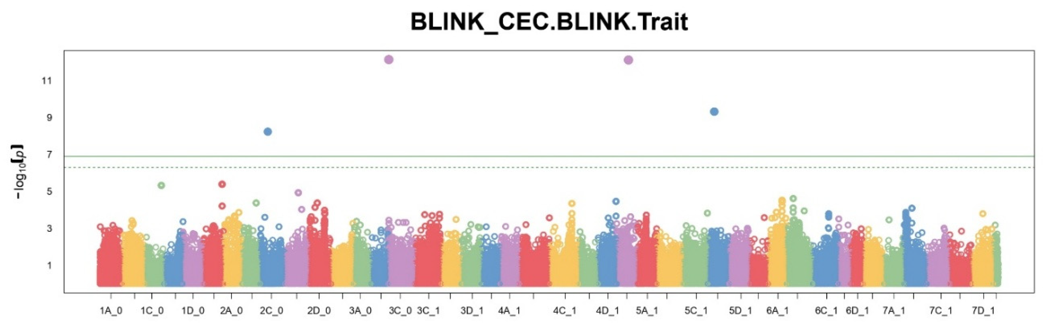
Figure 2.
Manhattan plot of GWAS results performed using the FarmCPU method. The X-axis shows chromosomes, and the Y-axis shows –log10(p)-values of association. The horizontal line indicates the significance threshold.
Figure 2.
Manhattan plot of GWAS results performed using the FarmCPU method. The X-axis shows chromosomes, and the Y-axis shows –log10(p)-values of association. The horizontal line indicates the significance threshold.
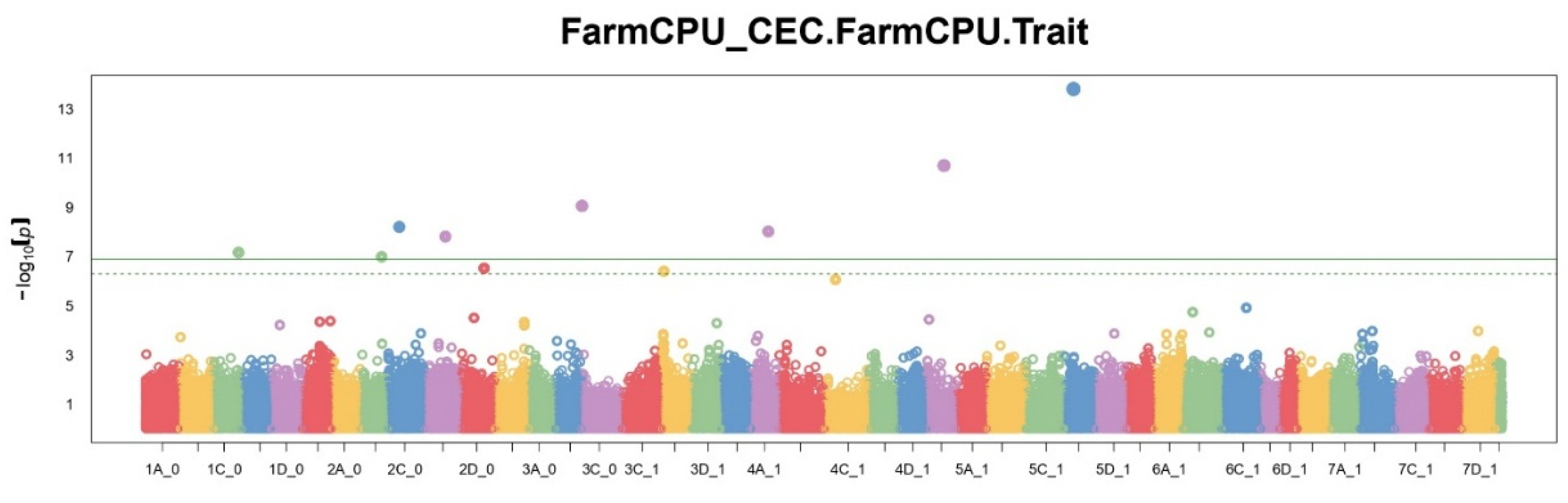
Figure 3.
Manhattan plot of GWAS results performed using the MLM method. The X-axis shows chromosomes, and the Y-axis shows the –log10(p)-values of the association. The horizontal line indicates the significance threshold.
Figure 3.
Manhattan plot of GWAS results performed using the MLM method. The X-axis shows chromosomes, and the Y-axis shows the –log10(p)-values of the association. The horizontal line indicates the significance threshold.
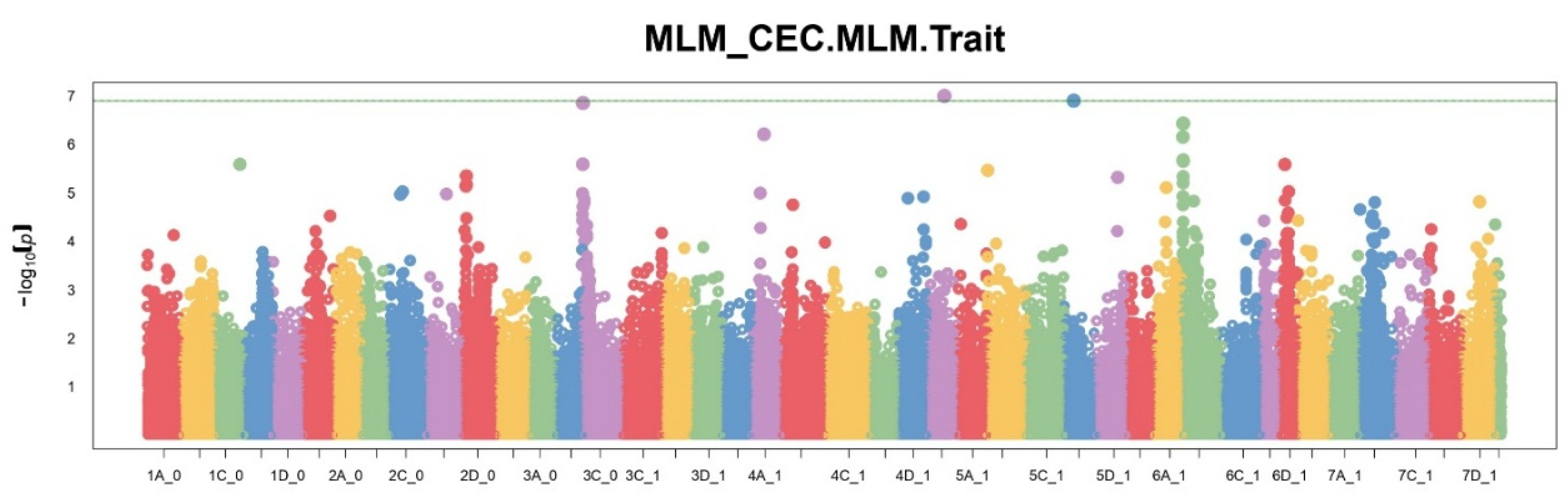
Figure 4.
Venn diagram showing the overlap of the top 100 SNPs between MLM, FarmCPU and BLINK methods.
Figure 4.
Venn diagram showing the overlap of the top 100 SNPs between MLM, FarmCPU and BLINK methods.
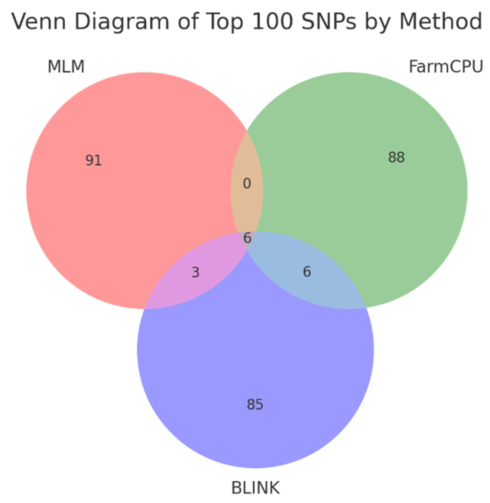
Figure 5.
QQ plots of p-value distributions for the three GWAS methods used to analyze the CEC trait in oats. a) FarmCPU; b) BLINK; c) MLM.
Figure 5.
QQ plots of p-value distributions for the three GWAS methods used to analyze the CEC trait in oats. a) FarmCPU; b) BLINK; c) MLM.
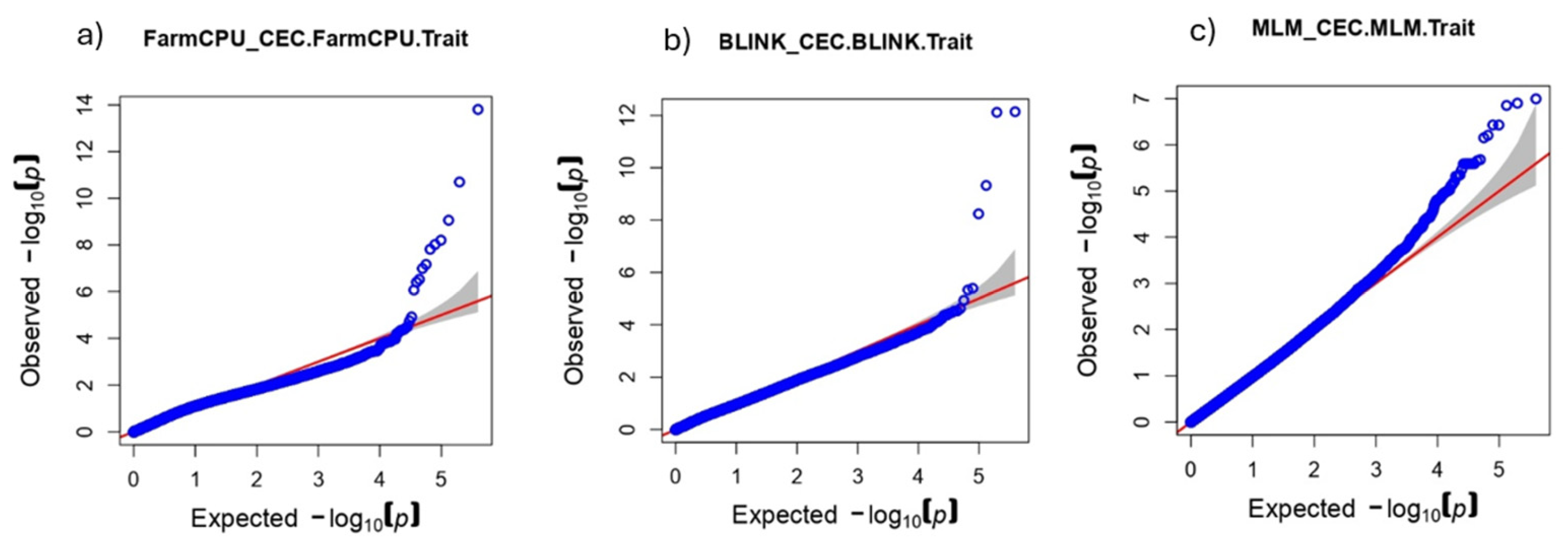
Figure 6.
Analysis of significant SNPs using the FarmCPU method: a) SNP significance vs. MAF; b) Estimated SNP effect vs. MAF; c) Explained phenotypic variance (%) vs. MAF.
Figure 6.
Analysis of significant SNPs using the FarmCPU method: a) SNP significance vs. MAF; b) Estimated SNP effect vs. MAF; c) Explained phenotypic variance (%) vs. MAF.
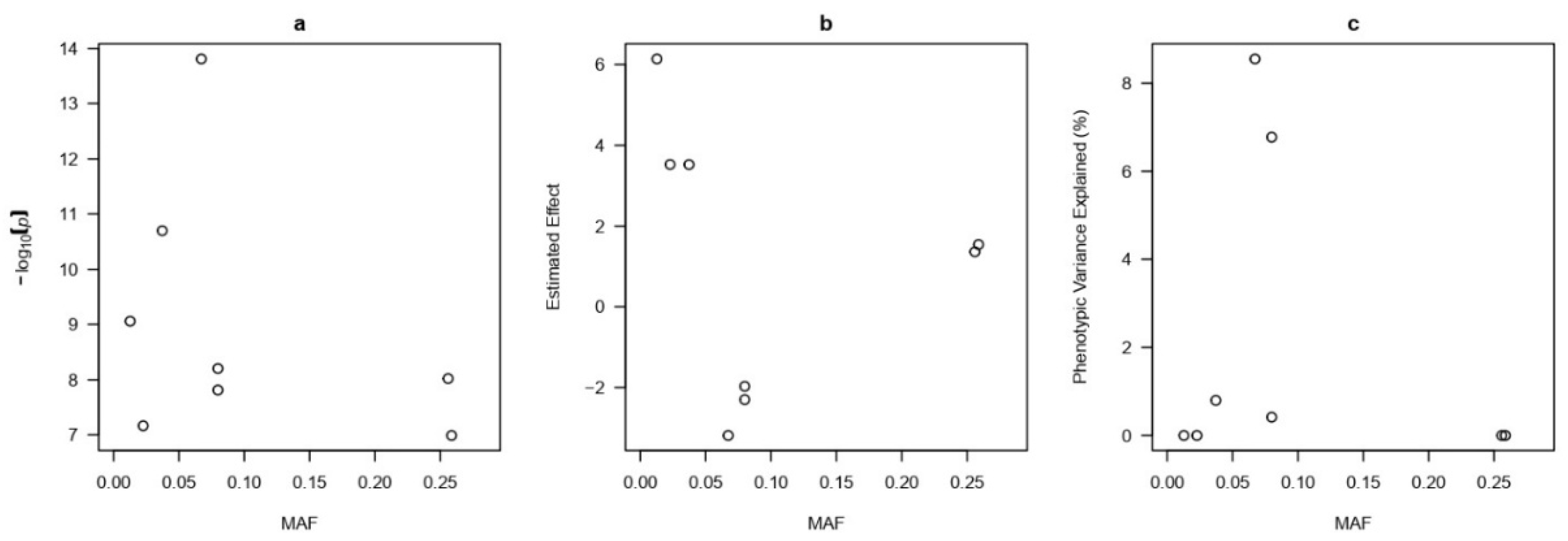
Figure 7.
Scree plot: percentage of variance explained by the first 10 principal components (PCA).
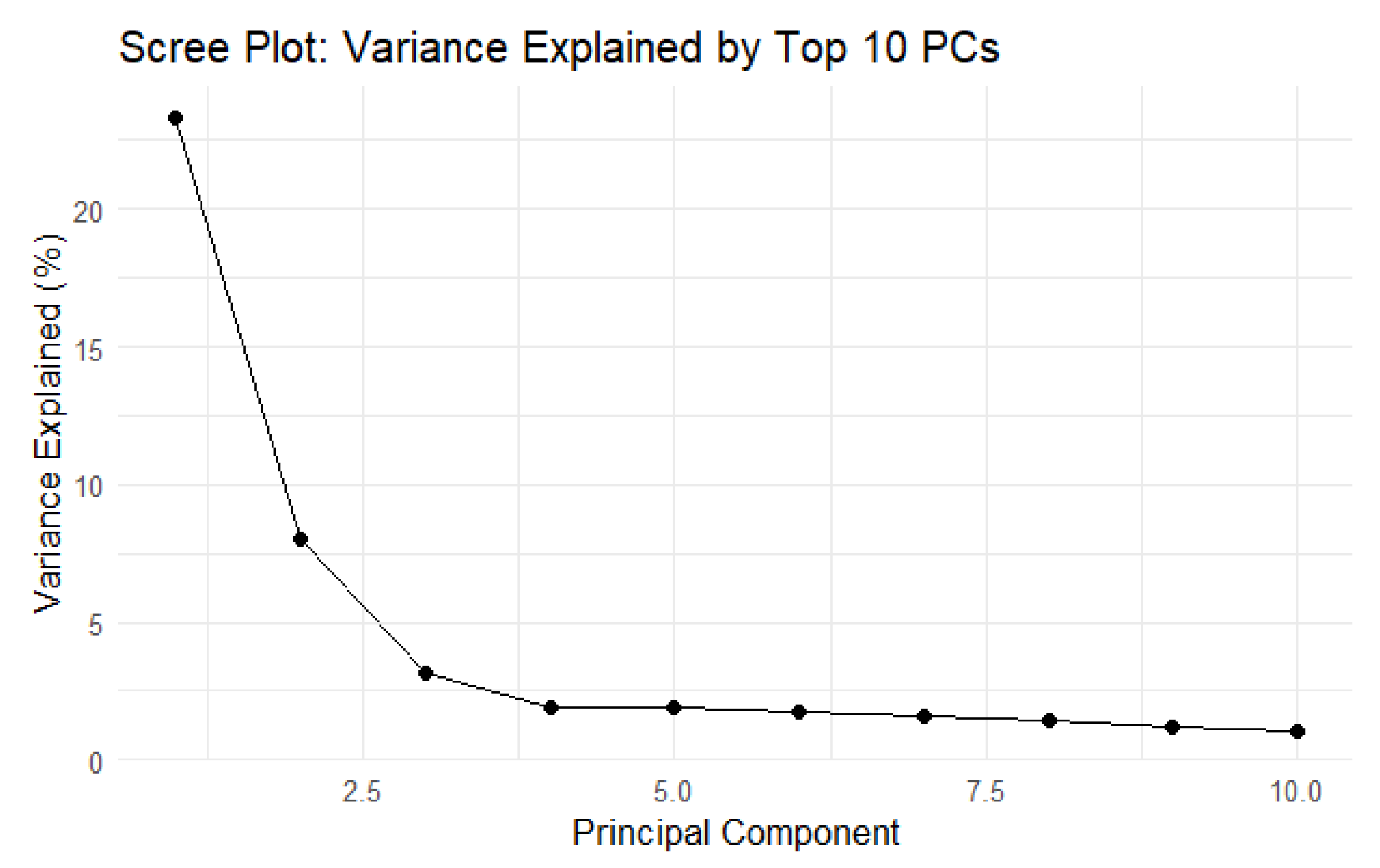

Table 1.
Top 10 SNPs identified by BayesCπ method with estimated effect and explained phenotypic variance proportion for CEC trait in oats (Avena sativa L.).
Table 1.
Top 10 SNPs identified by BayesCπ method with estimated effect and explained phenotypic variance proportion for CEC trait in oats (Avena sativa L.).
| SNP Index | Effect | Phenotypic Variance Explained (%) |
|---|---|---|
| 169477 | 0,003178171 | 11,44983 |
| 132785 | 0,003165221 | 12,29264 |
| 328532 | 0,003043769 | 10,89163 |
| 239964 | 0,002927365 | 11,48671 |
| 335052 | 0,002894788 | 11,51225 |
| 162400 | 0,002891 | 8,422963 |
| 122068 | 0,002886684 | 11,29919 |
| 289949 | 0,002851108 | 9,980992 |
| 47264 | 0,002825088 | 10,47982 |
| 393511 | 0,002824497 | 11,13786 |
Disclaimer/Publisher’s Note: The statements, opinions and data contained in all publications are solely those of the individual author(s) and contributor(s) and not of MDPI and/or the editor(s). MDPI and/or the editor(s) disclaim responsibility for any injury to people or property resulting from any ideas, methods, instructions or products referred to in the content. |
© 2025 by the authors. Licensee MDPI, Basel, Switzerland. This article is an open access article distributed under the terms and conditions of the Creative Commons Attribution (CC BY) license (http://creativecommons.org/licenses/by/4.0/).
Copyright: This open access article is published under a Creative Commons CC BY 4.0 license, which permit the free download, distribution, and reuse, provided that the author and preprint are cited in any reuse.


