
Submitted:
28 March 2025
Posted:
31 March 2025
You are already at the latest version
Abstract
Genome-wide association studies (GWAS) are essential for identifying genetic loci associated with complex traits, but the choice of statistical method significantly influences performance. This study systematically compared eight GWAS methods (GLM, MLM, CMLM, SUPER, MLMM, ECMLM, FarmCPU, and BLINK) in wheat, using simulated phenotypic data across 12 replicates to assess statistical power, false discovery rate (FDR), Type I error control, and computational efficiency. Phenotypes were simulated with a heritability of 0.7 and 10 quantitative trait nucleotides (QTNs) using genotypic data from 110 wheat accessions with 5,587 SNPs. Results indicated that multi-locus methods, particularly MLMM, FarmCPU, and BLINK, outperformed single-locus approaches, achieving higher power at lower FDR thresholds (MLMM: 0.434 at FDR = 0.0003; FarmCPU: 0.309 at FDR = 0.0007) and better Type I error control (MLMM: 0.943 at Type I error = 0.033; BLINK: 0.749 at Type I error = 0.073). MLMM exhibited the highest area under the curve (AUC) for power versus FDR (0.164 ± 0.105) and Type I error (0.823 ± 0.045), while FarmCPU and BLINK demonstrated superior computational efficiency, with runtimes of 10.03 ± 4.37 and 10.61 ± 3.67 seconds, respectively, compared to CMLM (52.86 ± 1.37 seconds). Manhattan and QQ plots confirmed better false positive control and p-value calibration for MLMM, FarmCPU, and BLINK. Conversely, traditional mixed models (MLM, CMLM) showed higher Type I error rates, and GLM exhibited elevated false positives. These findings underscore the robustness of multi-locus methods for wheat GWAS, particularly for traits with moderate to high heritability, and provide actionable guidelines for method selection, emphasizing MLMM for maximal power, FarmCPU for balanced performance, and BLINK for rapid, large-scale analyses. However, limitations in modeling polygenic traits and epistatic interactions, alongside wheat’s high linkage disequilibrium and polyploid nature, highlight the need for further research across diverse genetic architectures.
Keywords:
Computational efficiency
; False positive control
; GWAS
; Multi-locus methods
; Statistical power
; Type I error
; Wheat
1. Introduction
Genome-wide association studies (GWAS) have revolutionized genetics by enabling researchers to identify genetic loci associated with complex traits across diverse species (Liu et al. 2016). By linking phenotypic variation to genetic polymorphisms, GWAS have revealed variants associated with human diseases, such as type 2 diabetes, and agriculturally significant traits, such as drought tolerance in wheat, providing insights into genetic architecture and potential targets for breeding and therapeutic interventions (Visscher et al. 2017; Cebeci et al. 2023).
However, the exponential growth of genomic datasets encompassing millions of markers and individuals has intensified key challenges: balancing statistical power, controlling false discoveries, achieving high mapping resolution, and maintaining computational efficiency (Huang et al. 2019; Cebeci et al. 2023). In addition, the efficacy of GWAS hinges on statistical method selection, with approaches varying widely in their assumptions, computational demands, and ability to control confounding factors like population structure and familial relatedness (Kaler et al. 2020).
Over two decades, various methods have emerged with distinct trade-offs between statistical rigor and scalability. Traditional approaches such as general linear model (GLM) and mixed linear model (MLM) established the foundation for association mapping but face significant limitations. While computationally efficient, GLM often produces false positives by failing to account for population structure (Price et al. 2006). MLM addresses this by incorporating kinship matrices as random effects but demands higher computational resources and shows reduced power for small-effect loci (Segura et al. 2012; Wang et al. 2014). Advanced methods, including compressed MLM (CMLM) and enriched compressed MLM (ECMLM), improve efficiency by clustering individuals into groups and incorporating additional variance components (Zhang et al. 2010; Li et al. 2014), while multi-locus mixed models (MLMM) use stepwise regression to overcome these limitations (Segura et al. 2012; Wang et al. 2014). However, assumptions in methods like FarmCPU regarding the uniform distribution of quantitative trait nucleotides (QTNs) introduced biases in mapping resolution (da Silva Linge et al. 2022). Bayesian-information and linkage-disequilibrium iteratively nested keyway (BLINK) represented a significant advancement by replacing arbitrary binning with linkage disequilibrium (LD) guided covariate selection while eliminating costly random-effect computations (Huang et al. 2019).
Despite these developments, prior efforts to systematically compare GWAS methods have often focused on specific species or traits, leaving broader questions about method performance across diverse contexts unanswered (Tam et al. 2019). In addition, consensus on optimal methodologies remains elusive, with performance varying by species, trait architecture, and dataset scale (Wen et al. 2016). Challenges persist in inconsistent benchmarking of power-FDR trade-offs across thresholds, limited comparisons of mapping resolution, and unclear interactions between population structure covariates, model performance, and computational constraints such as memory usage and scalability of large datasets.
In crops like wheat, the complexity of the genome, including its polyploid nature (which complicates marker-trait associations due to multiple homoeologous genomes) and high levels of LD (which reduces mapping resolution by spreading signals across larger regions), presents unique challenges for effective gene mapping through GWAS. Recent investigations in wheat highlight persistent challenges with GWAS methods. In nested association mapping populations, BLINK demonstrated superior false positive control and computational efficiency, though its effectiveness for polygenic traits with epistatic interactions requires further investigation (Sandhu et al. 2024). These inconsistencies reveal a critical need for systematic comparison of GWAS methods across diverse genetic architectures, population structures, and computational constraints.
Thus, this study addresses these gaps by evaluating the statistical power, FDR, Type1 error, and computational efficiency of multiple GWAS methods using wheat genotypic data across 12 replications. By analyzing these models, we aim to provide practical insights into the strengths and limitations of each approach, guiding researchers toward informed methodological decisions in GWAS analyses.
2. Method
To evaluate the performance of various GWAS methods, we conducted a simulation study using the Genomic Association and Prediction Integrated Tool (GAPIT; Lipka et al. 2012) for wheat genotypic data in R. The analysis involved loading and cleaning genomic data, simulating phenotypes, performing GWAS with multiple methods, calculating performance metrics, and visualizing results.
2.1. Data Acquisition
Genotypic data for Triticum aestivum (bread wheat) accessions were downloaded from the T3 Wheat Database (https://wheat.triticeaetoolbox.org/breeders/download; Morales et al. 2022). The dataset included accessions from the HapMap2019 panel, genotyped using the Infinium 9K v2.1 protocol in Variant Call Format (VCF).
2.2. Data Preprocessing
The VCF file was converted into a numeric genotype matrix compatible with the GAPIT package in R using the `data.table` package to parse the file while skipping metadata headers. SNP map information (chromosome, position, and ID) was extracted into a myGM file, and genotype data were transformed into numeric values (0 = homozygous reference, 1 = heterozygous, 2 = homozygous alternate) using a custom function, with missing data coded as NA.
The initial genotype matrix (myGD) contained 110 individuals and 6538 SNPs, and the SNP map (myGM) included 6538 SNPs with chromosome and position information. SNPs with >50% missing data were removed, resulting in the exclusion of 951 SNPs, leaving 5587 SNPs for analysis. Given the relatively low remaining missing data rate (approximately 5.6%) and the often-intermediate nature of heterozygous calls in polyploid wheat, imputation with ’1’ (heterozygous) was chosen for the remaining missing values as a neutral default strategy to minimize potential bias. Chromosome names were standardized to the format “1A”, “1B”, ..., “7D” using a predefined mapping vector. Processed genotype (myGD.txt) and map (myGM.txt) files were saved as tab-delimited text files. Core R packages, including dplyr, tidyr, zoo, ggplot2, gridExtra, agricolae, pracma, and writexl, were used for preprocessing and analysis, alongside GAPIT functions sourced from http://zzlab.net/GAPIT/gapit_functions.txt.
2.3. Phenotype Simulation
The G2P function, sourced from http://zzlab.net/StaGen/2020/R/G2P.R, generated synthetic phenotypes with known quantitative trait nucleotides (QTNs). Parameters included heritability (h2 = 0.7), effect size component ( = 1), and the number of QTNs (NQTN =10), with QTN effects sampled from a normal distribution. For each replication (n = 12), QTNs were randomly selected, and genetic values were calculated as G = X, where X is the genotype matrix and is the effect size vector. Residual noise was added to achieve the target h2.
2.4. Genome-Wide Association Study (GWAS)
Eight GWAS models (GLM, MLM, CMLM, SUPER, MLMM, FarmCPU, BLINK, ECMLM) were evaluated using GAPIT package. Three principal components were included as covariates to control population structure. Window sizes for QTN proximity (1, 103, 104, 105 base pairs) were tested, chosen to span a range of distances to account for wheat’s high LD, which can extend over large genomic regions. Each model was run for 12 independent replications with a fixed random seed (seed = 99164) to ensure reproducibility, and computation time was recorded to assess efficiency.
2.5. Performance Metric Calculation
Metrics were computed for each combination of GWAS method, replication (n = 12), window size (1, 10³, 10⁴, 10⁵ base pairs), and significance threshold (determined by the GAPIT.FDR.TypeI function). For each method, the 12 GWAS results were iteratively processed using the GAPIT.FDR.TypeI function, sourced from http://zzlab.net/GAPIT/gapit_functions.txt, which evaluated power, FDR, and Type I error rate for all threshold-window combinations. Power was defined as the proportion of true QTNs detected within the specified window size of a known QTN, FDR as the proportion of false-positive SNPs among all significant SNPs, and Type I error rate as the proportion of non-QTN SNPs falsely deemed significant. To evaluate the trade-off between detection accuracy and error rates, the area under the curve (AUC) for Power vs. FDR and Power vs. Type I error was computed by GAPIT.FDR.TypeI.
This generated a data frame with columns: Method, Rep (replication index), WindowSize, Threshold, Power, FDR, and Type1_Error, AUC_FDR, and AUC_Type1. The final dataset comprised 8 methods × 12 replications × 4 window sizes × 10 thresholds = 3,840 rows. The integrity of data frame was validated by inspecting its structure, summary statistics, and consistency across replications to ensure accurate metric computation. Pairwise t-tests and Tukey’s Honestly Significant Difference (HSD) tests were applied to compare mean AUC values and computation times across methods, ensuring robust statistical comparisons of performance.
2.6. Visualization
Manhattan and QQ plots were generated for each method to visualize SNP associations and p-value distributions. Power-FDR and Power-Type I error curves were plotted after averaging results across replications. Box plots displayed AUC distributions, and bar plots illustrated mean computation times with standard errors. All visualizations were created using ggplot2 and saved as PNG files (300 dpi).
2.7. Software and Code Availability
The analysis was conducted in R version 4.3.1 (R core team, 2023). R script, processed genotype and map files are available upon request.
3. Results
This study compared the performance of eight GWAS methods (GLM, MLM, CMLM, SUPER, MLMM, ECMLM, FarmCPU, and BLINK) using simulated wheat phenotypic data across 12 replicates. Methods were evaluated based on statistical power, false FDR, Type I error control, AUC for power versus FDR and Type I error, computational efficiency, and visualization of GWAS signals.
3.1. Power, FDR, and Type I Error
The relationship between statistical power and FDR, as well as power and Type I error, was assessed (Figure 1-2). Multi-locus methods, MLMM and FarmCPU, exhibited the highest power at lower FDR thresholds (MLMM: 0.434 at FDR = 0.0003; FarmCPU: 0.309 at FDR = 0.0007), while GLM, MLM, CMLM, SUPER, and ECMLM showed higher FDR for comparable power levels (e.g., GLM: 0.783 at FDR = 0.048). BLINK achieved a balanced performance, with a power of 0.670 at FDR = 0.004. Power-FDR curves demonstrated that MLMM and FarmCPU achieved > 90% power at FDR thresholds below 0.2, whereas BLINK required higher FDR allowances (0.3–0.5) to reach comparable power. Conversely, single-locus methods like GLM and MLM exhibited steep declines in power at stringent FDR thresholds, with GLM showing 78% power at FDR = 0.1 but dropping to < 50% at FDR = 0.05.
For Type I error control, MLMM and FarmCPU outperformed other methods, maintaining high power with lower Type I error rates (MLMM: 0.943 at Type I error = 0.033; FarmCPU: 0.973 at Type I error = 0.119), while BLINK showed a balanced performance, achieving a power of 0.749 at a Type I error rate of 0.073. In contrast, GLM, MLM, CMLM, SUPER, and ECMLM exhibited higher Type I error rates at similar power levels (GLM: 0.998 at Type I error = 0.849). Type I error rates were tightly controlled by MLMM and FarmCPU, while traditional methods such as CMLM and ECMLM showed higher error rates, particularly at lenient significance thresholds.
3.2. AUC Analysis
The AUC_FDR and AUC_Type1 were calculated to provide a summary statistic for the overall performance of each method across a range of thresholds (Figure 3-Figure 4). For Power vs. FDR, a higher AUC indicates a better ability of the method to achieve high power while maintaining a low false discovery rate. Similarly, for Power vs. Type I error, a higher AUC signifies a better balance between detecting true positives and minimizing false positives.
For AUC_FDR, MLMM exhibited the highest mean (0.164 ± 0.105), followed by FarmCPU (0.117 ± 0.057) and BLINK (0.081 ± 0.048), while other methods (GLM: 0.015 ± 0.021; CMLM: 0.006 ± 0.010; MLM: 0.005 ± 0.005; SUPER: 0.005 ± 0.007; ECMLM: 0.005 ± 0.004) showed minimal FDR control, with significant differences among methods (ANOVA, p = 5.16 × 10⁻¹⁷).
For AUC_Type1, MLMM again performed best (0.823 ± 0.045), followed by FarmCPU (0.785 ± 0.092) and BLINK (0.749 ± 0.073), while GLM (0.500 ± 0.085), ECMLM (0.498 ± 0.082), SUPER (0.485 ± 0.071), MLM (0.475 ± 0.112), and CMLM (0.433 ± 0.077) had lower values, with significant differences (ANOVA, p = 1.42 × 10⁻26).
3.3. Computational Efficiency
Computational time varied significantly across methods (Figure 5). CMLM was the slowest (52.86 ± 1.37 seconds per replicate), followed by SUPER (44.74 ± 2.14 seconds), while FarmCPU (10.03 ± 4.37 seconds), BLINK (10.61 ± 3.67 seconds), and MLMM (10.05 ± 1.82 seconds) were the fastest. ECMLM (21.03 ± 1.87 seconds) and MLM (20.80 ± 1.92 seconds) showed moderate efficiency, whereas GLM (17.35 ± 1.47 seconds) outperformed mixed models but lagged behind multi-locus approaches. Notably, BLINK and FarmCPU achieved near-optimal power-FDR trade-offs with 4-5x faster speeds than CMLM and SUPER.
3.4. Manhattan and QQ Plots
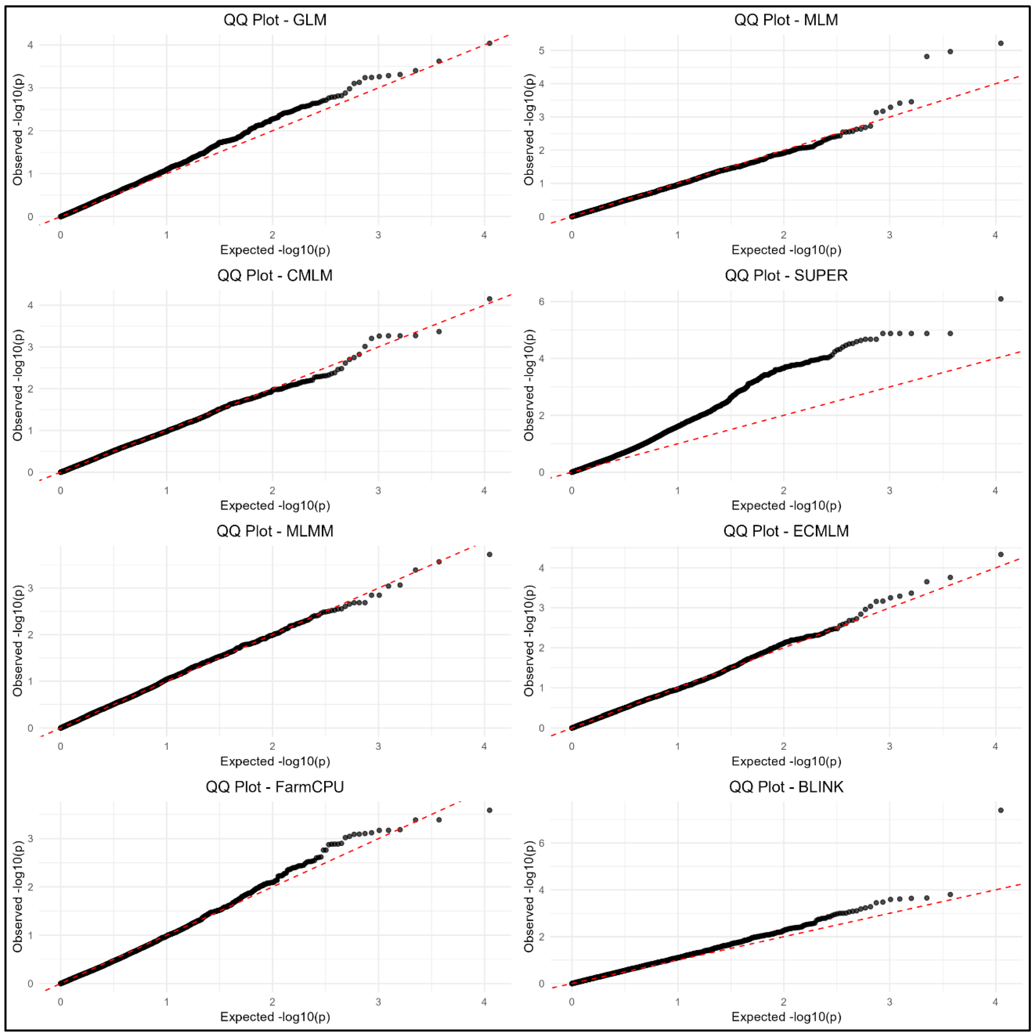
Manhattan plots (Figure 6) and QQ plots (Figure 7) were generated to visualize GWAS results. MLMM, FarmCPU, and BLINK showed clearer peaks near true QTN positions with less noise, indicating better control of false positives. GLM, MLM, CMLM, SUPER, and ECMLM exhibited more scattered signals, suggesting higher false positive rates, consistent with their elevated FDR and Type I error values.
QQ plots confirmed that MLMM, FarmCPU, and BLINK had better p-value calibration, with observed -log10(p) values closer to expected values under the null hypothesis.
4. Discussion
MLMM, FarmCPU, and BLINK consistently outperformed GLM, MLM, CMLM, SUPER, and ECMLM across most metrics, aligning with previous findings that multi-locus models (e.g., MLMM, FarmCPU) and Bayesian approaches (e.g., BLINK) better control false positives while maintaining high power (Liu et al. 2016; Huang et al. 2019). MLMM emerged as the most powerful method for controlling Type I error, likely due to its multi-locus stepwise regression that iteratively adjusts for confounding QTNs (Segura et al. 2012). Its superior AUC_FDR (0.164 ± 0.105) and AUC_Type1 (0.823 ± 0.045) suggest it effectively balances sensitivity and specificity. However, its computational speed lagged slightly behind FarmCPU and BLINK, which achieved comparable power with 80% faster runtimes.
FarmCPU’s strong and consistent performance in both power and speed underscores its utility for balanced workflows, corroborating its effectiveness in controlling both false positives and negatives (Liu et al. 2016). However, its assumption of uniformly distributed QTNs may explain occasional FDR inflation (da Silva Linge et al. 2022). BLINK’s efficiency aligns with its elimination of random-effects calculations and LD-based covariate selection (Huang et al. 2019), making it ideal for large-scale studies. While BLINK performed well overall, it showed more variability than MLMM and FarmCPU. BLINK’s variability may stem from uneven LD decay across wheat chromosomes, where weak LD regions reduce covariate selection accuracy. Additionally, using only three principal components might inadequately model population structure, inflating false positives in structured populations.
Single-locus methods (GLM, MLM, CMLM, SUPER, and ECMLM) exhibited higher FDR and Type I error rates, indicating poorer control of false positives. GLM’s simplicity, lacking correction for population structure, likely contributed to its high error rates (Price et al. 2006). Traditional mixed models (MLM, CMLM) incorporate kinship but struggle with complex traits involving multiple QTNs, as seen in their lower AUC values (Yu et al. 2006) and suffered from high Type I error and computational demands, consistent with known biases from overcorrected kinship matrices (Kaler et al. 2020). SUPER and ECMLM, despite their optimization for specific scenarios, did not outperform multi-locus methods, possibly due to the simulated trait’s complexity. Surprisingly, ECMLM - a compressed MLM variant, showed no significant improvement over CMLM. The lack of improvement in ECMLM over CMLM may be due to the simulated trait’s genetic architecture or wheat’s high LD, which could mask the benefits of enriched clustering, though this requires further investigation.
Computationally, FarmCPU, MLMM, and BLINK were the most efficient, making them practical for large-scale GWAS, whereas CMLM and SUPER’s longer runtimes (52.86 ± 1.37 and 44.74 ± 2.14 seconds, respectively) may limit their applicability in larger datasets, consistent with reports of their higher computational burden (Wang et al. 2014). For studies prioritizing statistical power, MLMM and FarmCPU are recommended, while BLINK offers the best balance of speed and accuracy. Researchers handling large datasets or requiring rapid iterations should favor BLINK or FarmCPU, whereas traditional mixed models (CMLM, MLM) are less advisable due to poor error control and inefficiency.
The superior performance of multi-locus methods (MLMM, FarmCPU, and BLINK) in balancing statistical power and Type I error control aligns with recent literature (Cebeci et al. 2023; Sandhu et al. 2024). These methods’ ability to account for both population structure and LD likely contribute to their enhanced performance. The consistency of MLMM across replicates suggests it may be particularly robust for wheat GWAS studies, especially for traits with moderate to high heritability. However, its computational demands should be considered for large datasets.
A key limitation of this study is the reliance on simulated phenotypes with fixed heritability (h² = 0.7) and pre-defined QTNs, which may not fully capture polygenic architectures or epistatic interactions. Similarly, the use of wheat data, characterized by high LD, limits generalizability to species with diverse genetic structures, such as outbred populations. The impact of varying degrees of population structure on method performance was not explicitly tested and warrants further investigation. Additionally, while the 5,587 SNPs used in this simulation study represent a reasonable marker density for evaluating GWAS methods, the results might be influenced by the specific number and distribution of these markers across the wheat genome. Future work should evaluate these methods across traits with varying heritability and genetic architectures, as well as in outbred populations by employing datasets with varying marker densities. Applying these methods to real wheat phenotypic data would further validate our findings and potentially reveal additional nuances in method performance.
5. Conclusions
In conclusion, our results strongly support the use of multi-locus methods, particularly MLMM, FarmCPU, and BLINK, for wheat GWAS studies due to their superior power, control of false positives, and computational efficiency. However, the choice of method should also consider computational resources, specific trait architecture, and research objectives. These findings provide actionable guidance for selecting GWAS methods tailored to specific experimental needs and lay a foundation for more informed decision-making in GWAS methodology selection for wheat and potentially other crop species with high LD, such as potato or cotton, where similar genomics challenges exist.
6. Acknowledgement
This work was conducted as part of Statistical Genomics 545, Spring 2025, at Washington State University, under the instruction of Dr. Zhiwu Zhang, with support from Meijing Liang. We thank Dr. Zhang and Meijing Liang for their guidance and feedback.
References
- Cebeci, Z., Bayraktar, M., & Gökçe, G. (2023). Comparison of the statistical methods for genome-wide association studies on simulated quantitative traits of domesticated goats (Capra hircus L.). Small Ruminant Research, 227, 107053. [CrossRef]
- da Silva Linge, C., Cai, L., Fu, W., Clark, J., Worthington, M., Rawandoozi, Z., ... & Gasic, K. (2022). Corrigendum: Multi-Locus Genome-Wide Association Studies Reveal Fruit Quality Hotspots in Peach Genome. Frontiers in Plant Science, 13, 879112. [CrossRef]
- Huang, M., Liu, X., Zhou, Y., Summers, R. M., & Zhang, Z. (2019). BLINK: a package for the next level of genome-wide association studies with both individuals and markers in the millions. Gigascience, 8(2), giy154. [CrossRef]
- Kaler, A. S., Gillman, J. D., Beissinger, T., & Purcell, L. C. (2020). Comparing different statistical models and multiple testing corrections for association mapping in soybean and maize. Frontiers in plant science, 10, 1794. [CrossRef]
- Lipka, A. E., Tian, F., Wang, Q., Peiffer, J., Li, M., Bradbury, P. J., ... & Zhang, Z. (2012). GAPIT: genome association and prediction integrated tool. Bioinformatics, 28(18), 2397-2399. [CrossRef]
- Li, M., Zhang, Y. W., Zhang, Z. C., Xiang, Y., Liu, M. H., Zhou, Y. H., ... & Zhang, Y. M. (2022). A compressed variance component mixed model for detecting QTNs and QTN-by-environment and QTN-by-QTN interactions in genome-wide association studies. Molecular Plant, 15(4), 630-650. [CrossRef]
- Liu, X., Huang, M., Fan, B., Buckler, E. S., & Zhang, Z. (2016). Iterative usage of fixed and random effect models for powerful and efficient genome-wide association studies. PLoS genetics, 12(2), e1005767. [CrossRef]
- Nicolas Morales, Jean-Luc Jannink, Clay L. Birkett, David J Waring, Lukas A Mueller, et. al. (2022) Breedbase: a digital ecosystem for modern plant breeding, G3 Genes|Genomes|Genetics,12(7), jkac078, . [CrossRef]
- Price, A. L., Patterson, N. J., Plenge, R. M., Weinblatt, M. E., Shadick, N. A., & Reich, D. (2006). Principal components analysis corrects for stratification in genome-wide association studies. Nature genetics, 38(8), 904-909. [CrossRef]
- R Core Team. R: A language and environment for statistical computing.(2023) R foundation for statistical computing, Vienna, Austria. https://www.R-project.org/.
- Sandhu, K. S., Burke, A. B., Merrick, L. F., Pumphrey, M. O., & Carter, A. H. (2024). Comparing performances of different statistical models and multiple threshold methods in a nested association mapping population of wheat. Frontiers in Plant Science, 15, 1460353. [CrossRef]
- Segura, V., Vilhjálmsson, B. J., Platt, A., Korte, A., Seren, Ü., Long, Q., & Nordborg, M. (2012). An efficient multi-locus mixed-model approach for genome-wide association studies in structured populations. Nature genetics, 44(7), 825-830. [CrossRef]
- Tam, V., et al. (2019). Benefits and limitations of genome-wide association studies. Nature Reviews Genetics, 20(8), 467-484. [CrossRef]
- Visscher, P. M., et al. (2017). 10 Years of GWAS Discovery: Biology, Function, and Translation. American Journal of Human Genetics, 101(1), 5-22. [CrossRef]
- Wang, Q., Tian, F., Pan, Y., Buckler, E. S., & Zhang, Z. (2014). A SUPER powerful method for genome wide association study. PloS one, 9(9), e107684. [CrossRef]
- Wen, Y. J., Zhang, H., Zhang, J., Feng, J. Y., Huang, B., Dunwell, J. M., ... & Wu, R. (2016). A fast multi-locus random-SNP-effect EMMA for genome-wide association studies. bioRxiv, 077404. [CrossRef]
- Yu, J., Pressoir, G., Briggs, W. H., Vroh Bi, I., Yamasaki, M., Doebley, J. F., ... & Buckler, E. S. (2006). A unified mixed-model method for association mapping that accounts for multiple levels of relatedness. Nature genetics, 38(2), 203-208. [CrossRef]
- Zhang, Z., Ersoz, E., Lai, C. Q., Todhunter, R. J., Tiwari, H. K., Gore, M. A., ... & Buckler, E. S. (2010). Mixed linear model approach adapted for genome-wide association studies. Nature genetics, 42(4), 355-360. [CrossRef]
Figure 1.
Power vs. False Discovery Rate (FDR) curves for eight GWAS methods.
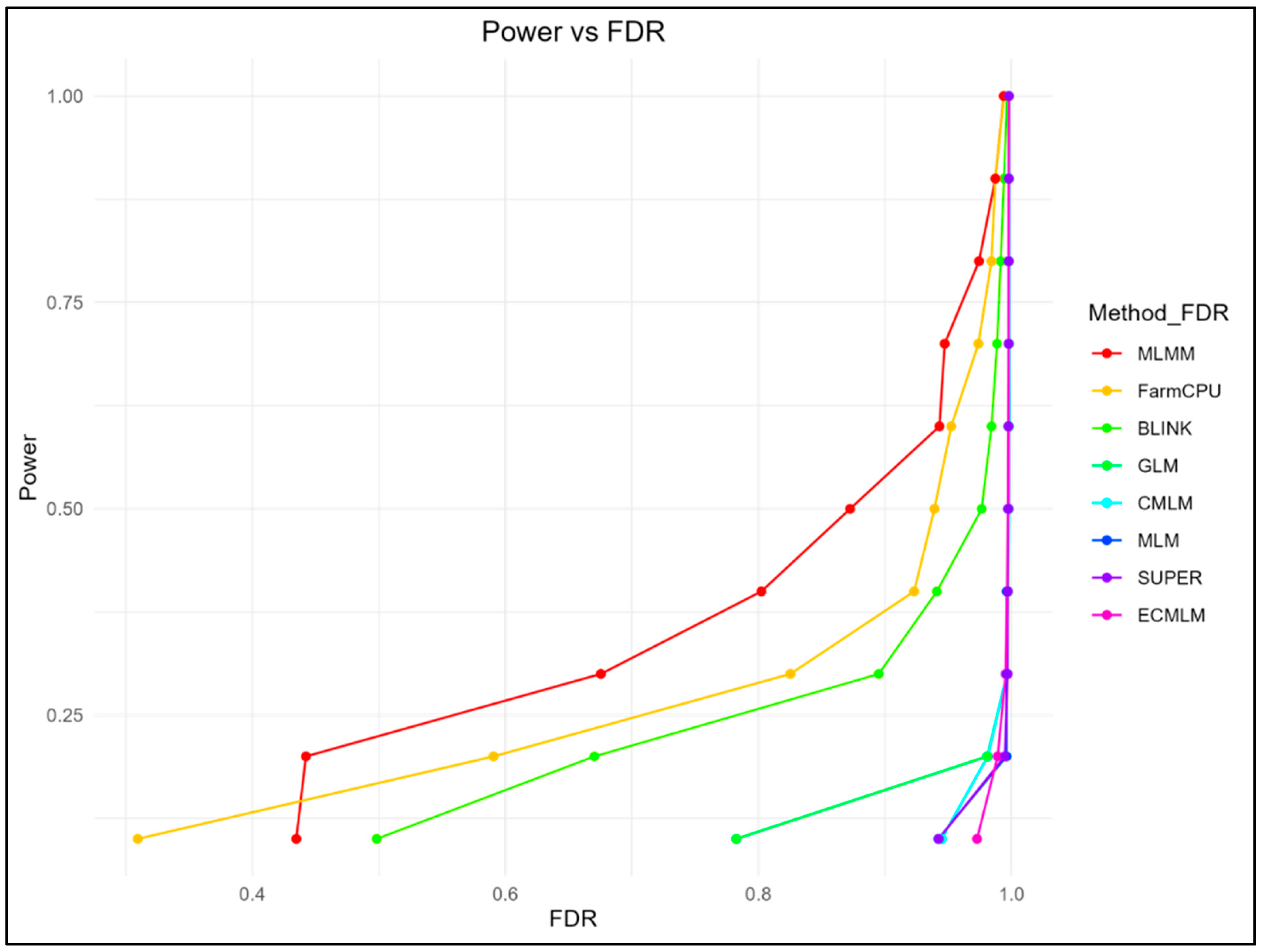
Figure 2.
Power vs. Type I Error curves for eight GWAS methods.
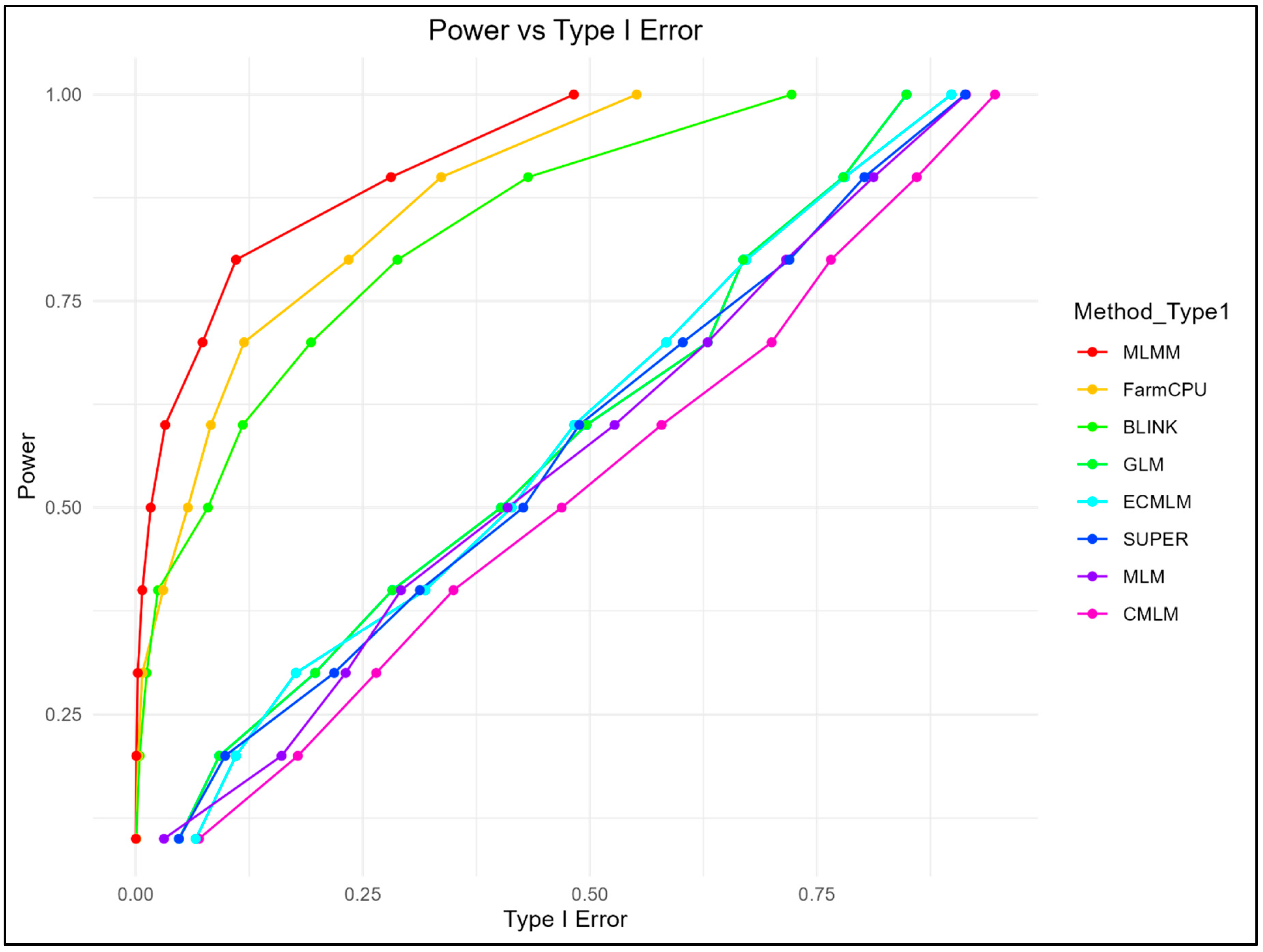
Figure 3.
Area under the curve (AUC) for Power vs. FDR across methods.
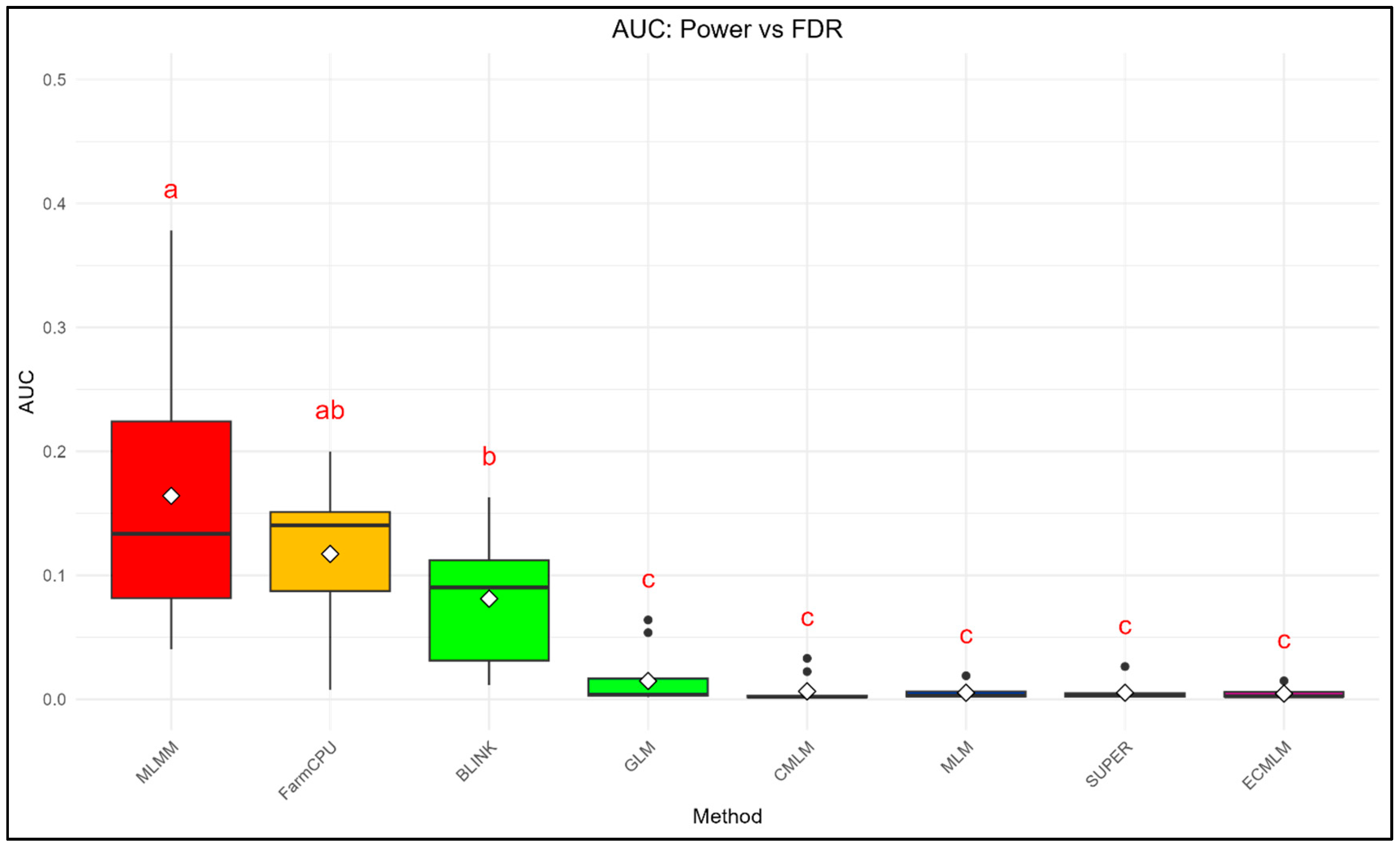
Figure 4.
Area under the curve (AUC) for Power vs. Type I Error across methods.
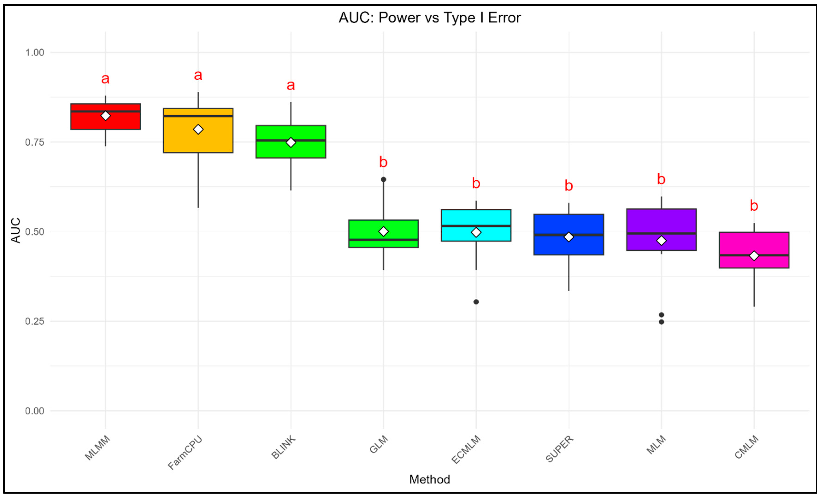
Figure 5.
Computational time (seconds per replication) for GWAS methods.
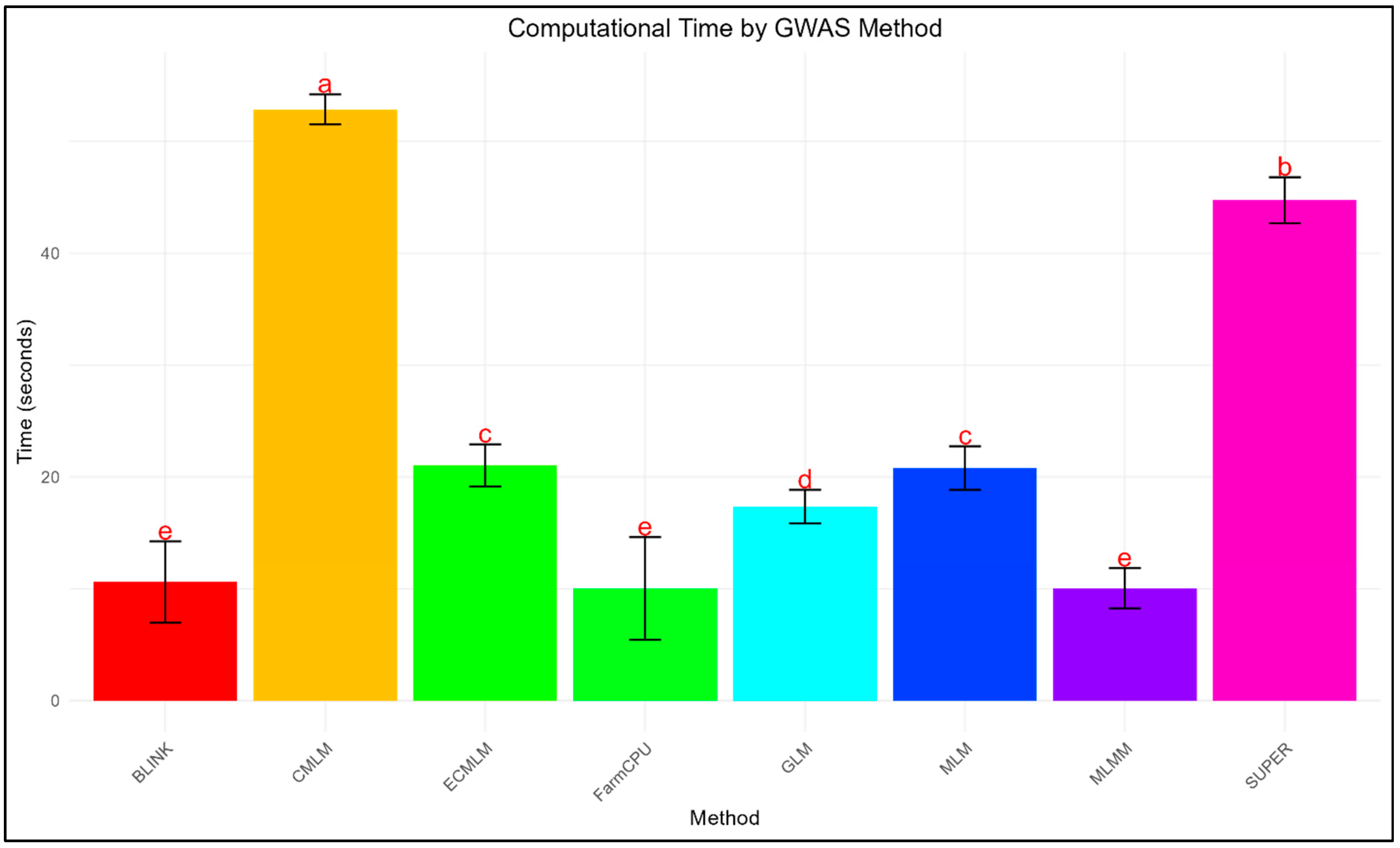
Figure 6.
Stacked Manhattan plots of GWAS results for eight methods.
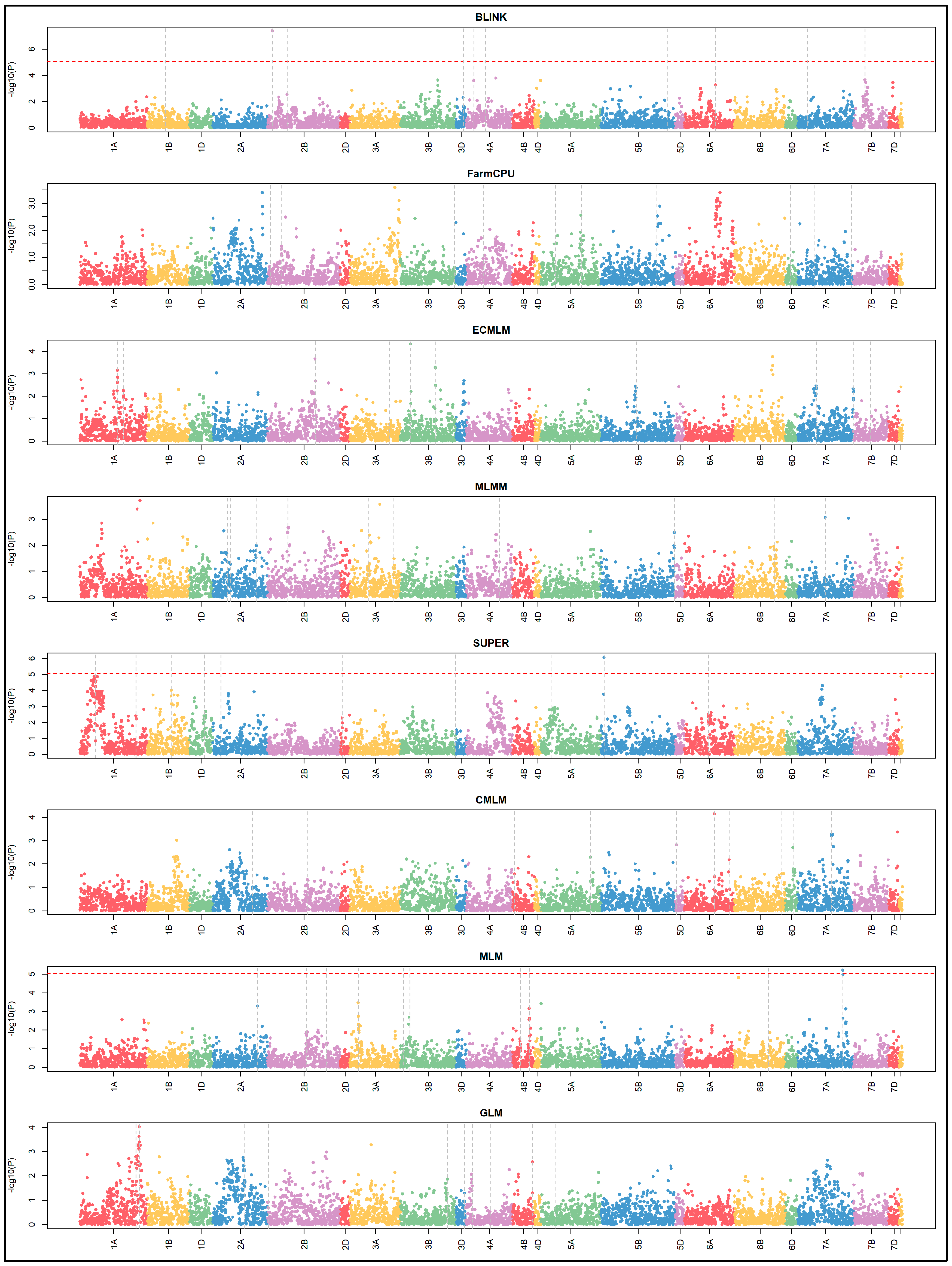
Figure 7.
Quantile-quantile (QQ) plots of p-value distributions for eight methods.
Disclaimer/Publisher’s Note: The statements, opinions and data contained in all publications are solely those of the individual author(s) and contributor(s) and not of MDPI and/or the editor(s). MDPI and/or the editor(s) disclaim responsibility for any injury to people or property resulting from any ideas, methods, instructions or products referred to in the content. |
© 2025 by the authors. Licensee MDPI, Basel, Switzerland. This article is an open access article distributed under the terms and conditions of the Creative Commons Attribution (CC BY) license (http://creativecommons.org/licenses/by/4.0/).
Copyright: This open access article is published under a Creative Commons CC BY 4.0 license, which permit the free download, distribution, and reuse, provided that the author and preprint are cited in any reuse.


