
Submitted:
30 March 2025
Posted:
31 March 2025
You are already at the latest version
Abstract
Genome-Wide Association Studies (GWAS) are pivotal for identifying quantitative trait nucleotides (QTNs) in crops like barley. However, the performance of different methods varies depending on population structure and computational demands. This study compared eight GWAS methods (GLM, MLM, CMLM, SUPER, MLMM, FarmCPU, BLINK, and ECMLM) using a simulated dataset from the World Barley Core Collection (WBCC) with 6,332 SNPs, 318 samples, a heritability of 0.7, and 15 QTNs across 30 replicates. Statistical power, false discovery rate (FDR), Type I error, and computational efficiency were evaluated at a 10 Mb window size through Power vs FDR/Type I error curves, Area Under the Curve (AUC) boxplots, QQ plots, Manhattan plots, and timing bar graphs. MLMM consistently outperformed other methods in balancing power and error control, followed closely by BLINK and FarmCPU, which also demonstrated high mapping resolution in Manhattan plots. GLM exhibited the highest false-positive rate, as seen in its QQ plot, while ECMLM underperformed despite theoretical advantages. GLM and MLMM were the fastest, whereas CMLM was the slowest, highlighting significant computational trade-offs. These findings suggest that MLMM is ideal for high-quality QTN discovery in barley, while BLINK offers a balanced approach for routine analyses. The study provides a framework for selecting GWAS methods in barley, emphasizing the importance of balancing power, error control, and computational efficiency in structured populations like the WBCC.
Keywords:
false discovery rate
; mapping resolution
; population structure
; QTN detection
; Type I error
; World Barley Core Collection
Introduction
Genome-wide association studies (GWAS) identify statistical associations between molecular markers and quantitative traits, offering a promising approach for revealing the genetic basis of phenotypic variation (Bradbury et al., 2011). The first GWAS study was published in 2005, marking the exponential growth of this approach over time. GWAS have become indispensable in plant genomics, offering a robust framework to identify genetic variants associated with complex agronomic traits. By exploiting natural genetic variation within diverse populations, GWAS enabled the discovery of marker-trait associations that underpin marker-assisted selection and genomic selection, key strategies in modern crop improvement. This approach holds immense promises for addressing global challenges such as food security and malnutrition, particularly through biofortification, the enhancement of nutritional content in staple crops like barley. The broad appeal of GWAS stems from its potential to deliver climate-resilient and nutritionally superior varieties, making it a focal point for researchers, breeders, and agricultural stakeholders worldwide (X. Huang & Han, 2014; Mackay et al., 2009).
A persistent challenge in GWAS is the selection of an appropriate statistical model that optimizes the detection of true associations while minimizing false positives and computational demands. Early models, such as the General Linear Model (GLM), provide a straightforward approach to associating genetic markers with phenotypes but fail to account for population structure and relatedness, often resulting in elevated false discovery rates (FDR; Price et al., 2006). In contrast, the Mixed Linear Model (MLM) incorporates kinship matrices and population structure covariates to reduce spurious associations, albeit at the cost of reduced statistical power (Yu et al., 2006). This trade-off complicates the analysis of datasets like the World Barley Core Collection (WBCC), a globally diverse panel selected for its potential in barley biofortification, where accurate identification of quantitative trait nucleotides is critical for breeding success.
Significant efforts have been made to refine GWAS methodologies, yielding a spectrum of models with distinct strengths. The Compressed MLM (CMLM) enhances computational efficiency by clustering individuals based on genetic similarity, while the Enriched CMLM (ECMLM) further optimizes kinship to boost power (Lipka et al., 2012; Zhang et al., 2010). Multi-locus models, such as the MLMM (Multiple Loci Mixed Model), SUPER (Settlement of MLM Under Progressively Exclusive Relationship), FarmCPU (Fixed and random model Circulating Probability Unification), and BLINK (Bayesian-information and Linkage-disequilibrium Iteratively Nested Keyway), address confounding between covariates and testing markers, improving resolution and power (Huang et al., 2019; Liu et al., 2016; Segura et al., 2012; S.-B. Wang et al., 2016). These advancements, integrated into tools like the Genome Association and Prediction Integrated Tool (GAPIT), reflect a concerted push to tailor GWAS to diverse plant populations, including the WBCC, which offers extensive genetic variation for studying biofortification traits (Lipka et al., 2012).
Despite these innovations, a comprehensive evaluation of these models’ performance remains lacking, particularly for datasets like the WBCC, which is poised to advance barley nutritional enhancement. The relative merits of single-locus models (e.g., GLM, MLM, CMLM, ECMLM) versus multi-locus models (e.g., SUPER, MLMM, FarmCPU, BLINK) vary across populations, and computational efficiency often conflicts with statistical robustness (Huang et al., 2019). This uncertainty hinders researchers’ ability to select the optimal model for the WBCC, where balancing power, FDR, mapping resolution, and runtime are essential for identifying reliable marker-trait associations.
This study seeks to bridge this knowledge gap by systematically comparing eight GWAS models (GLM, MLM, CMLM, SUPER, MLMM, FarmCPU, BLINK, and ECMLM) using simulated data modeled after the filtered 6,332 SNPs of the WBCC. The objective of the study is (i) to assess statistical power relative to FDR and Type I error, clarifying each model’s accuracy in detecting true associations; (ii) to evaluate mapping resolution through Manhattan and quantile-quantile plots, to determine precision in localizing genetic variants; and (iii) to measure computational efficiency, providing practical insights for large-scale analyses. These findings aim to guide plant breeders and geneticists in selecting the most effective GWAS approach, enhancing the precision and efficiency of genetic discovery for barley biofortification.
Materials and Methods
Data Curation
This study utilized genotypic data from the WBCC, comprising 318 barley (Hordeum vulgare L.) lines. The dataset included 9K SNP markers generated using the Illumina Infinium iSelect 9K Barley SNP array, with marker positions aligned to the Morex v3 reference genome. The genotypic data were sourced from the Triticeae Toolbox (https://triticeaetoolbox.org/barley/?old=old) and subjected to stringent quality filtering to ensure reliability. Markers with missing data exceeding 10% across lines, lines with more than 30% missing marker data, and markers with a minor allele frequency below 5% were excluded. This filtering process retained 6,332 high-quality SNP markers for subsequent analysis.
To evaluate the performance of GWAS models, phenotypic data were simulated based on the filtered genotypic dataset. Simulations were conducted using the GAPIT.Phenotype.Simulation function within the GAPIT framework (Lipka et al., 2012). Phenotypes were generated with a heritability (h²) of 0.7, incorporating 15 quantitative trait nucleotides (QTNs) with an effect size of 0.6, following a normal distribution. A total of 30 replicates were conducted for each of the eight GWAS methods, with a seed (99164) set for reproducibility. QTN positions were recorded for each replicate to evaluate true positives in subsequent analyses.
Statistical Models for GWAS
GWAS was conducted using GAPIT (Lipka et al., 2012) where the eight GWAS models (GLM, MLM, CMLM, SUPER, MLMM, FarmCPU, BLINK, and ECMLM) were evaluated. Analyses were conducted using genotypic data, marker information, simulated phenotypic data, and three principal components to account for population structure. Each model was executed for all 30 simulation replicates, with true QTN positions recorded to assess detection accuracy. Computational runtime was measured to capture the duration of each GAPIT run per model and replicate.
Statistical Power, FDR, and Type I Error Calculation
Statistical power, FDR, and Type I error were calculated using the GAPIT.FDR.TypeI function across four window sizes (1, 1,000, 10,000, and 100,000 base pairs) to evaluate model performance under varying genomic resolutions. Input included the marker information, true QTN positions, and GWAS results. Power was defined as the proportion of true QTNs detected, FDR as the ratio of false positives to total positives, and Type I error as the rate of false positives among null markers. Metrics were aggregated across replicates for each model and window size, focusing on the 10 Mb window for final statistical tests due to its relevance for barley genomic studies (Comadran et al., 2012).
Statistical Comparisons
Analysis of variance (ANOVA) was performed to test significant differences in Area Under the Curve (AUC; Power vs FDR and Power vs Type I Error) and computational runtime across the eight methods. Post-hoc mean separation was conducted with Tukey’s Honestly Significant Difference (HSD) test at a 5% significance level (alpha = 0.05) from the agricolae package. Mean separation letters were assigned to indicate statistically distinct groups for each metric.
Data Visualization
Visualization was performed in R to illustrate model performance. AUC plots of power versus FDR and power versus Type I error were generated using base R graphics, with lines colored by model. Boxplots of power and FDR distributions were created to show variability across replicates. Computational runtime was visualized as a bar graph with error bars (mean ± standard error), sorted by mean runtime. Power versus FDR and Type I error curves were plotted for each model with 10Mb window size. Manhattan plots and quantile-quantile (QQ) plots were produced for each model using GWAS results.
Software and Environment
Analyses were performed in R (version 4.3.1) (R Core Team, 2023) using the following packages: GAPIT for GWAS, dplyr and tidyr for data manipulation (Wickham et al., 2023), ggplot2 and gridExtra for visualization (Wickham, 2016; Auguie, 2017), agricolae for statistical tests (Lopez & Lopez, 2023), pracma for AUC calculation (Hassani, 2023), and zoo for rolling means (Zeileis & Grothendieck, 2005). All metrics, including AUC values, computational times, and aggregated statistics, were exported to an Excel file using the writexl package (Ooms, 2023) for further analysis. All scripts were sourced from the ZZLab repository (http://zzlab.net) (Zhang, 2020).
Results
The comparison of the eight GWAS models (GLM, MLM, CMLM, SUPER, MLMM, FarmCPU, BLINK, and ECMLM) revealed distinct differences in statistical power, FDR, Type I error, mapping resolution, and computational efficiency when applied to a dataset of 6,332 SNPs across 318 WBCC samples with simulated phenotypes.
Statistical power versus FDR and Type I Error Curves
The Power vs FDR plot (Figure 1a) illustrates the trade-off between statistical power and FDR across the eight methods at varying significance thresholds. MLMM consistently achieved the highest power at lower FDR levels, reaching a power of 0.845 with an FDR of 0.578, followed by FarmCPU (power = 0.876, FDR = 0.677) and BLINK (power = 0.875, FDR = 0.656). GLM exhibited the steepest FDR increase, achieving a power of 0.891 but with a high FDR of 0.712, indicating poor control of false positives. MLM (power = 0.875, FDR = 0.634), CMLM (power = 0.877, FDR = 0.673), SUPER (power = 0.874, FDR = 0.631), and ECMLM (power = 0.876, FDR = 0.657) showed intermediate performance, with FDR rising more gradually than GLM but less optimally than MLMM.
While FDR measures the proportion of false positives among significant results, Type I error (false-positive rate) reflects the proportion of false positives among null hypotheses, as further evidenced by the QQ plots (Figure 3). The Power vs Type I Error plot (Figure 1b) similarly highlights MLMM’s superior balance, reaching a power of 0.845 with a Type I error of 0.578 at threshold 15, followed by BLINK (power = 0.875, Type I = 0.656) and FarmCPU (power = 0.876, Type I = 0.677). GLM again showed the highest error rate (power = 0.891, Type I = 0.712), while MLM (power = 0.875, Type I = 0.634), CMLM (power = 0.877, Type I = 0.673), SUPER (power = 0.874, Type I = 0.631), and ECMLM (power = 0.876, Type I = 0.657) maintained lower Type I errors than GLM but higher than MLMM, consistent with their FDR trends.
AUC for Power versus FDR and Type I Error
The AUC: Power vs FDR boxplot (Figure 2a) quantifies the overall performance of each method in balancing power and FDR across all thresholds. MLMM exhibited the highest median AUC of 0.674 ± 0.123, with a tight interquartile range (IQR) indicating consistent performance across replicates. BLINK and FarmCPU followed with median AUCs of 0.628 ± 0.105 and 0.614 ± 0.082, respectively, but their wider IQRs suggest greater variability compared to MLMM. GLM had the lowest median AUC of 0.424 ± 0.154, with a wide IQR and several outliers, reflecting its high variability and poor error control. MLM, CMLM, SUPER, and ECMLM showed intermediate performance with median AUCs of 0.507 ± 0.118, 0.497 ± 0.091, 0.494 ± 0.137, and 0.460 ± 0.083, with SUPER displaying the most variability due to its larger IQR. ANOVA confirmed significant differences across methods (p = 2.55 × 10⁻²⁰).
The AUC: Power vs Type I Error boxplot (Figure 2b) showed a similar hierarchy, with MLMM leading at a median AUC of 0.849 ± 0.057, followed by BLINK (0.834 ± 0.045) and FarmCPU (0.820 ± 0.049), both showing tight IQRs and consistent performance. SUPER, MLM, and CMLM had median AUCs of 0.811 ± 0.048, 0.803 ± 0.048, and 0.799 ± 0.048, respectively, while ECMLM (0.777 ± 0.063) and GLM (0.767 ± 0.071) were the lowest, with GLM again showing high variability through its wide IQR and outliers. ANOVA indicated significant variation (p = 5.55 × 10⁻⁹), and the boxplots underscore MLMM’s robustness and GLM’s sensitivity to simulation conditions.
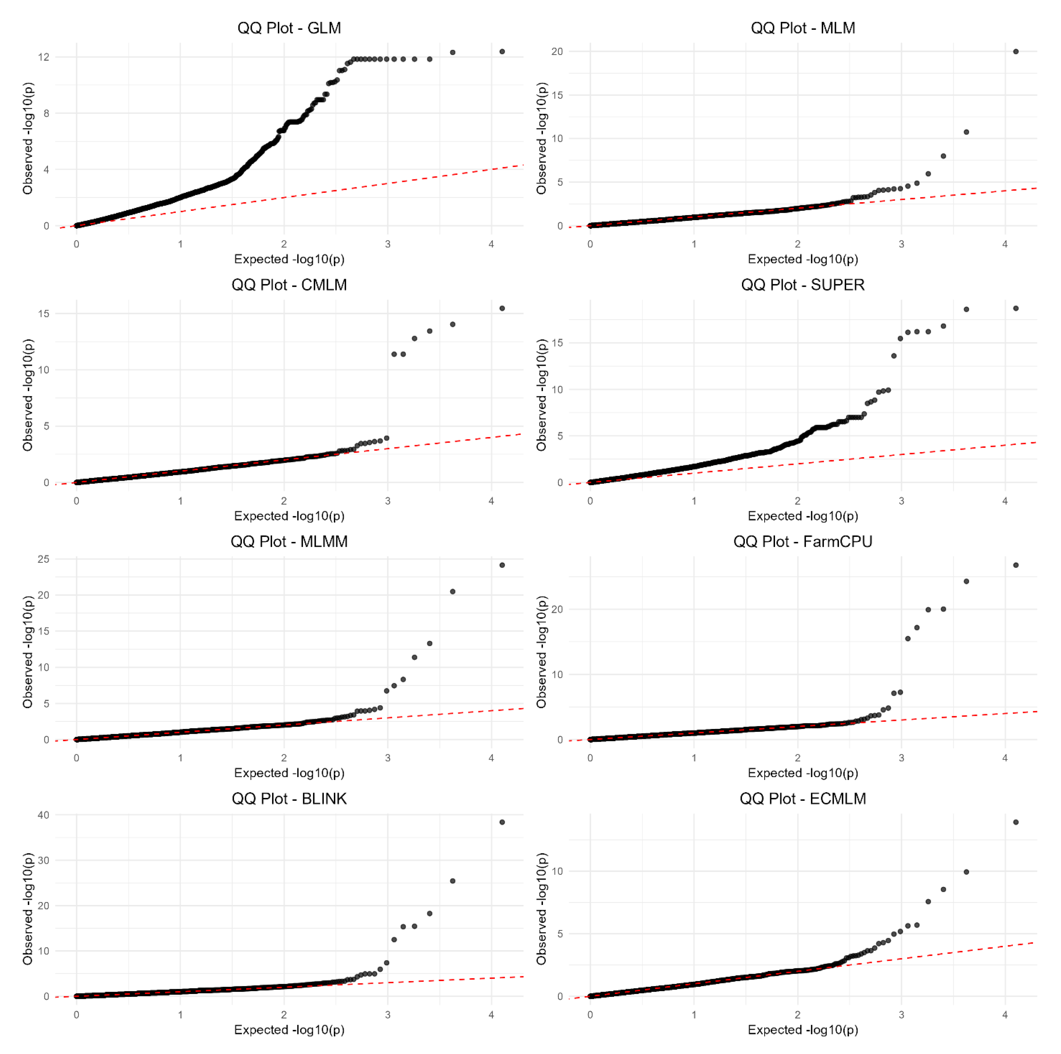
QQ Plots (False-Positive Control)
The QQ plots (Figure 3) compare observed -log10(p) values against expected -log10(p) values under the null hypothesis, revealing each method’s ability to control false positives. GLM’s plot exhibited a pronounced upward deviation from the diagonal line (y = x) starting at expected -log10(p) values above 2, with observed values reaching up to 12, indicating a high rate of false positives across the p-value spectrum. MLM, CMLM, SUPER, MLMM, FarmCPU, BLINK, and ECMLM showed better control, with their observed -log10(p) values more closely following the diagonal line, though slight deviations occurred at higher expected values, where observed -log10(p) reached 5–10 for MLM, FarmCPU, and BLINK, suggesting minor inflation of p-values at stricter thresholds. MLMM and FarmCPU displayed the least deviation, with their curves hugging the diagonal most closely, indicating effective false-positive control even at higher expected values. GLM’s significant deviation underscores its inability to account for population structure, leading to consistently inflated p-values across replicates.
Figure 3.
QQ plots for eight GWAS methods using a simulated dataset from the World Barley Core Collection (WBCC) with 6,332 SNPs, 318 samples, h² = 0.7, and 15 QTNs across 30 replicates. Each plot compares observed -log10(p) values against expected -log10(p) values under the null hypothesis, with a red dashed diagonal line (y = x) indicating ideal false-positive control.
Manhattan Plots (Mapping Resolution)
The stacked Manhattan plots (Figure 4) displayed -log10(p) values across chromosomes for each method, with a significance threshold at approximately -log10(p) = 5. BLINK and FarmCPU exhibited the sharpest peaks, with significant SNPs concentrated in specific regions (e.g., chromosomes 1, 3, and 7), suggesting high mapping resolution and precise QTN detection, as their peaks were narrow and well-defined. MLMM also showed distinct peaks, but with slightly broader bases, indicating moderate resolution compared to BLINK and FarmCPU. GLM’s plot revealed numerous significant SNPs scattered across all chromosomes, with broader and less defined peaks, reflecting lower resolution and a tendency for over-detection, consistent with its high false-positive rate in the QQ plot. MLM, CMLM, SUPER, and ECMLM displayed intermediate resolution, with fewer significant SNPs than GLM but less precision than BLINK and FarmCPU, as their peaks were more dispersed and less sharply defined. The distribution of significant SNPs generally aligned with the simulated QTN positions, though GLM’s over-detection suggests sensitivity to the WBCC’s population structure, leading to false positives across non-QTN regions.
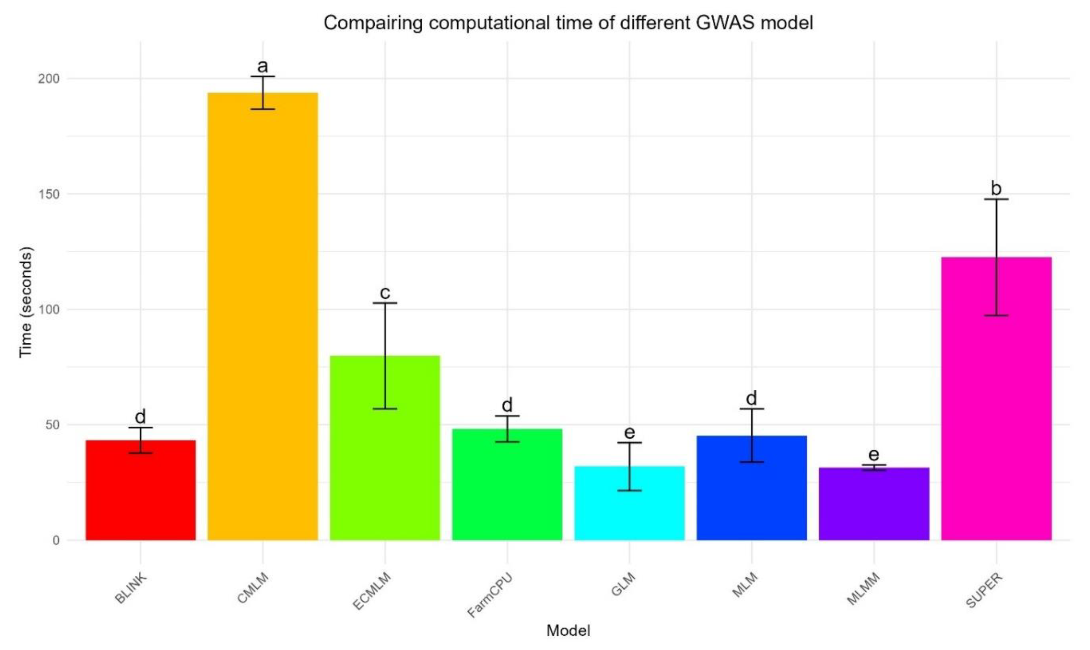
Computational Speed
The timing bar graph (Figure 5) illustrates the computational efficiency of each method across 30 replicates, with mean times and standard deviations highlighting distinct trends. GLM was the fastest, with a mean runtime of 29.8 ± 9.3 seconds, showing a tight distribution of runtimes and minimal variability. MLMM followed closely at 31.4 ± 1.3 seconds, with an even tighter distribution, indicating consistent performance. BLINK achieved a mean runtime of 43.1 ± 5.9 seconds, while FarmCPU was slightly slower at 48.0 ± 5.5 seconds, both showing moderate variability in their runtimes. SUPER (45.8 ± 2.2 seconds) and MLM (48.0 ± 5.5 seconds) showed moderate runtimes, with SUPER exhibiting less variability. ECMLM was slower at 96.0 ± 5.5 seconds, and CMLM was the slowest at 193.8 ± 7.2 seconds, with both showing wider distributions, indicating greater variability in computational demand across replicates. ANOVA confirmed significant differences across methods (p = 1.62 × 10⁻¹³⁷), and Tukey’s HSD distinguished five groups, underscoring CMLM’s substantial computational burden compared to the faster methods like GLM and MLMM.
Discussion
This study systematically compared eight GWAS methods (GLM, MLM, CMLM, SUPER, MLMM, FarmCPU, BLINK, and ECMLM) using simulated data from the WBCC, revealing distinct differences in their ability to balance statistical power, error control, mapping resolution, and computational efficiency. MLMM emerged as the top performer, achieving the highest statistical power while effectively controlling false positives, as evidenced by its superior Power vs FDR (AUC: 0.674 ± 0.123) and Power vs Type I Error (AUC: 0.849 ± 0.057) curves (Figure 1a,b and Figure 2a,b). This aligns with Segura et al. (2012), who demonstrated MLMM’s efficacy in structured populations through its multi-locus framework, which iteratively fits QTNs to reduce confounding effects. BLINK and FarmCPU followed closely, showing strong power and high mapping resolution with sharp peaks in their Manhattan plots (Figure 4), supporting Liu et al. (2016) and Huang et al. (2019), who noted that simultaneous marker testing enhances power in populations with complex LD patterns like barley. However, MLMM’s edge over BLINK contrasts with Huang et al. (2019), who suggested BLINK’s LD-based refinement might outperform with denser marker sets, indicating that the WBCC’s 6,332 SNP density may favor MLMM’s approach.
GLM exhibited the poorest performance, with significant deviations in its QQ plot (Figure 3) and broad peaks in its Manhattan plot (Figure 4), reflecting a high false-positive rate (Type I error). This is consistent with Kang et al. (2008), who highlighted GLM’s inability to correct for population structure, a critical limitation in the diverse WBCC (Comadran et al., 2012). MLM and CMLM showed moderate performance, benefiting from kinship adjustments but constrained by their single-locus frameworks, aligning with Yu et al. (2006) and Zhang et al. (2010), though their limitations compared to multi-locus methods echo Liu et al. (2016). SUPER and ECMLM underperformed, with less precise QTN detection in their Manhattan plots. SUPER’s results align with Wang et al. (2016), who noted its binning strategy can miss QTNs in regions with moderate LD, while ECMLM’s poor performance contradicts Zhang et al. (2010), who emphasized its theoretical advantages in structured populations, possibly due to overfitting in the WBCC’s moderate marker density. However, ECMLM slightly outperformed GLM in AUC for Power vs FDR (0.460 vs 0.424) and Power vs Type I Error (0.777 vs 0.767), challenging its expected superiority.
Computationally, GLM and MLMM were the fastest, with mean runtimes of 29.8 ± 9.3 seconds and 31.4 ± 1.3 seconds, respectively (Figure 5), mirroring Wang et al. (2014) in maize and suggesting that these patterns may generalize across cereals. MLMM’s speed advantage over Segura et al. (2012) likely stems from GAPIT’s optimization, while GLM’s efficiency reflects its simple fixed-effect model. BLINK (43.1 ± 5.9 seconds) was faster than FarmCPU (48.0 ± 5.5 seconds) without significant power loss, validating Huang et al. (2019) and highlighting its suitability for routine analyses. In contrast, CMLM’s high runtime (193.8 ± 7.2 seconds) reflects its computational burden, consistent with Zhang et al. (2010), due to its compressed kinship matrix scaling poorly with the WBCC’s 318 samples.
MLMM’s success likely results from its ability to model multiple QTNs simultaneously, capturing the WBCC’s moderate LD structure without overfitting. BLINK and FarmCPU’s performance stems from their iterative marker selection and cofactor adjustments, which mitigate confounding in structured populations. GLM’s high false-positive rate arises from its lack of population structure correction, a significant drawback in the WBCC’s diverse genetic background. MLM and CMLM’s moderate results reflect their kinship-based adjustments, which control false positives better than GLM but are less suited for complex traits due to their single-locus approach. SUPER’s binning strategy may miss QTNs in moderate LD regions, while ECMLM’s extended model may be too complex for the WBCC’s marker density, leading to overfitting. BLINK’s speed advantage over FarmCPU highlights its algorithmic improvements, making it a practical choice for large-scale studies.
This study offers several novel contributions. It provides the first comprehensive evaluation of ECMLM in barley, revealing its limitations in the WBCC context despite slight improvements over GLM. It also quantifies power-runtime trade-offs using standardized WBCC data (Figure 2a,b and Figure 5), enabling barley breeding programs to make informed cost-benefit decisions. Furthermore, it validates BLINK’s computational efficiency for routine barley analyses, extending prior findings to a new crop context, and underscores the importance of multi-locus models like MLMM and BLINK for accurate QTN detection in barley’s diverse genetic background.
Despite its strengths, this study has limitations. The simulated phenotypes may not fully capture the complexity of real barley traits, such as epistatic interactions or environmental influences, which could affect method performance. The 6,332 SNP dataset, while representative, may limit mapping resolution compared to modern high-density arrays (e.g., 50K SNPs or whole-genome resequencing), potentially underestimating methods like BLINK and FarmCPU that excel with denser markers. Additionally, the findings are specific to the WBCC, and results may vary across barley populations with different genetic architectures, such as landraces or breeding panels.
Future studies should validate these findings with real phenotypic datasets to assess each method’s ability to identify biologically relevant QTNs, particularly for complex traits like yield, disease resistance, and nutritional content in barley breeding. Expanding to higher-density SNP arrays could provide deeper insights into BLINK and FarmCPU’s robustness for polygenic traits. Investigating GWAS methods across diverse barley populations will help determine the generalizability of these conclusions. Finally, integrating multi-trait GWAS approaches, and machine learning-based models could further enhance QTN detection, refining method selection for barley breeding programs.
Conclusions
This study provides a comprehensive comparison of eight GWAS methods using the WBCC, offering key insights into their suitability for QTN detection. MLMM emerged as the most effective method, balancing statistical power and error control, making it ideal for high-stakes gene discovery in structured barley populations. BLINK and FarmCPU also performed well, with BLINK's computational efficiency making it preferable for routine analyses. Conversely, GLM’s high false positive rate and ECMLM’s unexpected underperformance highlight their limitations. The computational trade-offs observed emphasize method selection based on resource constraints. These findings support MLMM for QTN discovery and BLINK for genomic selection, while future studies should validate these trends using denser SNP arrays and diverse genetic architectures to refine barley breeding strategies.
Acknowledgement
The author gratefully acknowledges Dr. Zhiwu Zhang, instructor of Statistical Genomics, for his guidance and expertise in designing and overseeing this course. The author also sincerely thanks the Teaching Assistant, Meijing Liang, for her patient support, detailed feedback, and assistance in resolving technical challenges during this assignment.
References
- Auguie, B. (2017). gridExtra: Miscellaneous Functions for "Grid" Graphics. R package version 2.3. Available online: https://CRAN.R-project.
- Bradbury, P. , Parker, T., Hamblin, M. T., & Jannink, J.-L. Assessment of Power and False Discovery Rate in Genome-Wide Association Studies using the BarleyCAP Germplasm. Crop Science 2011, 51, 52–59. [Google Scholar] [CrossRef]
- Comadran, J. , Kilian, B., Russell, J., Ramsay, L., Stein, N., Ganal, M., Shaw, P., Bayer, M., Thomas, W., Marshall, D., Hedley, P., Tondelli, A., Pecchioni, N., Francia, E., Korzun, V., Walther, A., & Waugh, R. Natural variation in a homolog of Antirrhinum CENTRORADIALIS contributed to spring growth habit and environmental adaptation in cultivated barley. Nature Genetics 2012, 44, 1388–1392. [Google Scholar] [CrossRef] [PubMed]
- Hassani, H. (2023). pracma: Practical Numerical Math Functions. R package version 2.4.2. Available online: https://CRAN.R-project.
- Huang, M. , Liu, X., Zhou, Y., Summers, R. M., & Zhang, Z. BLINK: A package for the next level of genome-wide association studies with both individuals and markers in the millions. GigaScience 2019, 8, giy154. [Google Scholar] [CrossRef] [PubMed]
- Huang, X. , & Han, B. Natural Variations and Genome-Wide Association Studies in Crop Plants. Annual Review of Plant Biology 2014, 65, 531–551. [Google Scholar] [CrossRef] [PubMed]
- Kang, H. M. , Zaitlen, N. A., Wade, C. M., Kirby, A., Heckerman, D., Daly, M. J., & Eskin, E. Efficient Control of Population Structure in Model Organism Association Mapping. Genetics 2008, 178, 1709–1723. [Google Scholar] [CrossRef] [PubMed]
- Lipka, A. E. , Tian, F., Wang, Q., Peiffer, J., Li, M., Bradbury, P. J.,... & Zhang, Z. GAPIT: Genome association and prediction integrated tool. Bioinformatics 2012, 28, 2397–2399. [Google Scholar] [CrossRef] [PubMed]
- Liu, X. , Huang, M., Fan, B., Buckler, E. S., & Zhang, Z. Iterative Usage of Fixed and Random Effect Models for Powerful and Efficient Genome-Wide Association Studies. PLOS Genetics 2016, 12, e1005767. [Google Scholar] [CrossRef]
- Lopez, O. , & Lopez, F. (2023). agricolae: Statistical Procedures for Agricultural Research. R package version 1.3-5. Available online: https://CRAN.R-project.
- Mackay, T. F. C. , Stone, E. A., & Ayroles, J. F. The genetics of quantitative traits: Challenges and prospects. Nature Reviews Genetics 2009, 10, 565–577. [Google Scholar] [CrossRef] [PubMed]
- Ooms, J. (2023). writexl: Export Data Frames to Excel 'xlsx' Format. R package version 1.2. Available online: https://CRAN.R-project.
- Price, A. L. , Patterson, N. J., Plenge, R. M., Weinblatt, M. E., Shadick, N. A., & Reich, D. Principal components analysis corrects for stratification in genome-wide association studies. Nature Genetics 2006, 38, 904–909. [Google Scholar] [CrossRef] [PubMed]
- R Core Team. (2023). R: A Language and Environment for Statistical Computing. R Foundation for Statistical Computing, Vienna, Austria. Available online: https://www.R-project.
- Segura, V. , Vilhjálmsson, B. J., Platt, A., Korte, A., Seren, Ü., Long, Q., & Nordborg, M. An efficient multi-locus mixed-model approach for genome-wide association studies in structured populations. Nature Genetics 2012, 44, 825–830. [Google Scholar] [CrossRef] [PubMed]
- Wang, Q. , Tian, F., Pan, Y., Buckler, E. S., & Zhang, Z. A SUPER powerful method for genome-wide association study. PLoS ONE 2016, 11, e0157771. [Google Scholar] [CrossRef]
- Wang, S. B. , Feng, J. Y., Ren, W. L., Huang, B., Zhou, L., Wen, Y. J.,... & Zhang, Z. Improving power and accuracy of genome-wide association studies via a multi-locus mixed linear model methodology. Scientific Reports 2014, 6, 19444. [Google Scholar] [CrossRef]
- Wickham, H. (2016). ggplot2: Elegant Graphics for Data Analysis. Springer-Verlag, New York. Available online: https://ggplot2.tidyverse.
- Wickham, H. , Vaughan, D., & Girlich, M. (2023). tidyr: Tidy Messy Data and dplyr: A Grammar of Data Manipulation. R package versions 1.3.0 and 1.1.2, respectively. Available online: https://CRAN.R-project.org/package=tidyr. https://CRAN.R-project.
- Yu, J. , Pressoir, G., Briggs, W. H., Vroh Bi, I., Yamasaki, M., Doebley, J. F., McMullen, M. D., Gaut, B. S., Nielsen, D. M., Holland, J. B., Kresovich, S., & Buckler, E. S. A unified mixed-model method for association mapping that accounts for multiple levels of relatedness. Nature Genetics 2006, 38, 203–208. [Google Scholar] [CrossRef] [PubMed]
- Zeileis, A. , & Grothendieck, G. zoo: S3 Infrastructure for Regular and Irregular Time Series. Journal of Statistical Software 2005, 14, 1–27. [Google Scholar] [CrossRef]
- Zhang, Z. (2020). ZZLab: Resources for Statistical Genomics. Available online: http://zzlab.
- Zhang, Z. , Ersoz, E., Lai, C. Q., Todhunter, R. J., Tiwari, H. K., Gore, M. A.,... & Buckler, E. S. Mixed linear model approach adapted for genome-wide association studies. Nature Genetics 2010, 42, 355–360. [Google Scholar] [CrossRef] [PubMed]
Figure 1.
a: Power vs FDR curves for eight GWAS methods using a simulated dataset from the World Barley Core Collection (WBCC) with 6,332 SNPs, 318 samples, h² = 0.7, and 15 QTNs across 30 replicates. The plot shows the trade-off between statistical power and false discovery rate (FDR) at varying significance thresholds (0 to 1), with each method represented by a distinct color. b: Power vs Type I Error curves for eight GWAS methods using a simulated dataset from the World Barley Core Collection (WBCC) with 6,332 SNPs, 318 samples, h² = 0.7, and 15 QTNs across 30 replicates. The plot illustrates the relationship between statistical power and Type I error at varying significance thresholds (0 to 1), with each method represented by a distinct color.
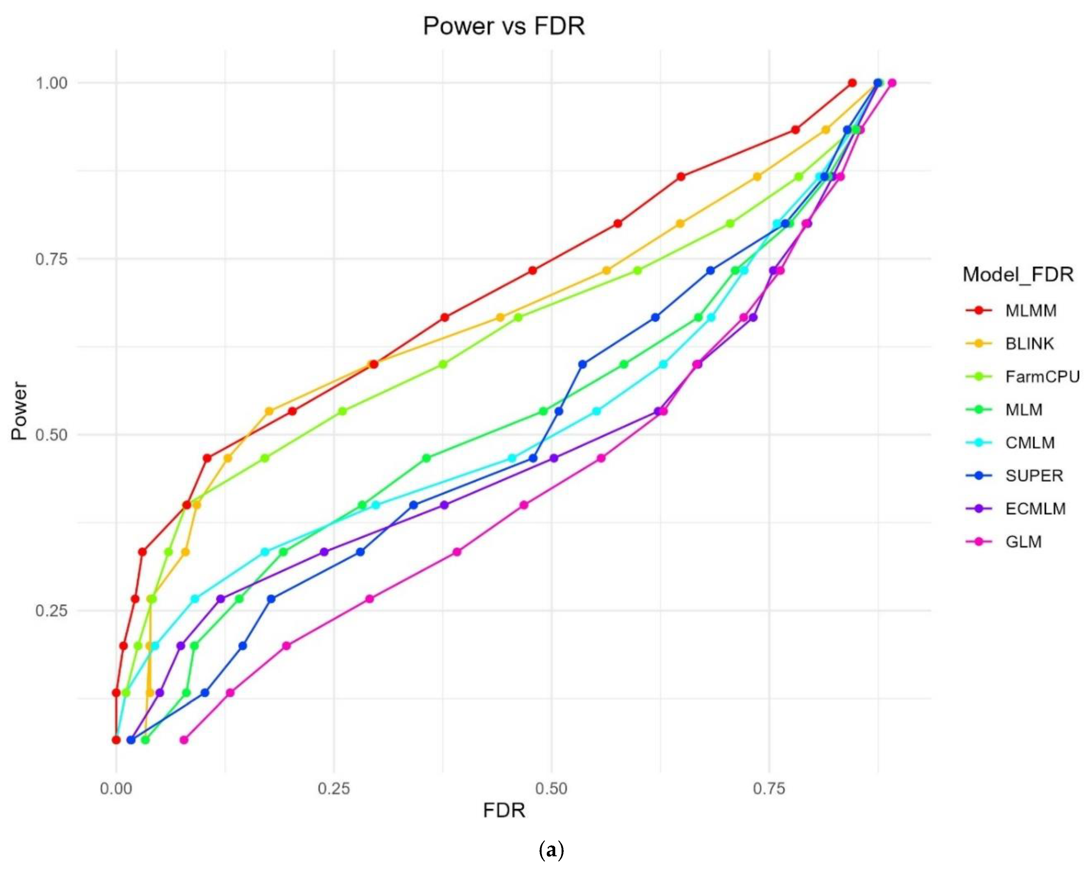
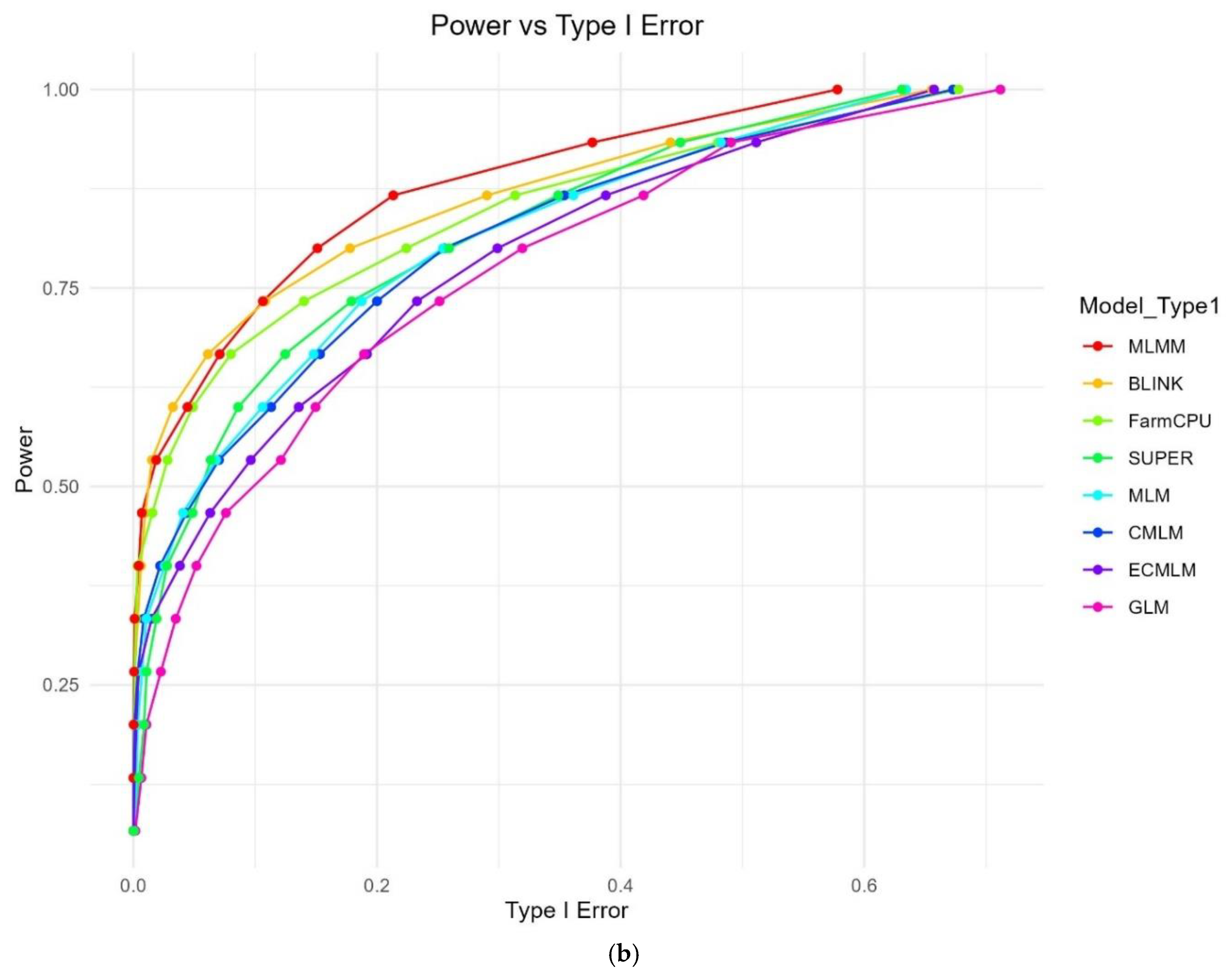
Figure 2.
a: Boxplot of AUC (Power vs FDR) for eight GWAS methods using a simulated dataset from the World Barley Core Collection (WBCC) with 6,332 SNPs, 318 samples, h² = 0.7, and 15 QTNs across 30 replicates at a 10 Mb window size. Each box represents the distribution of AUC values, with mean separation letters (a–b) assigned by Tukey’s HSD test (p = 2.55 × 10⁻²⁰). b: Boxplot of AUC (Power vs Type I Error) for eight GWAS methods using a simulated dataset from the World Barley Core Collection (WBCC) with 6,332 SNPs, 318 samples, h² = 0.7, and 15 QTNs across 30 replicates at a 10 Mb window size. Each box represents the distribution of AUC values, with mean separation letters (a–c) assigned by Tukey’s HSD test (p = 5.55 × 10⁻⁹).
Figure 4.
Stacked Manhattan plots for eight GWAS methods using a simulated dataset from the World Barley Core Collection (WBCC) with 6,332 SNPs, 318 samples, h² = 0.7, and 15 QTNs across 30 replicates. Each plot displays -log10(p) values across chromosomes (1–7), with chromosomes color-coded, and a red dashed line indicating the significance threshold at approximately -log10(p) = 5. Vertical gray dashed lines mark simulated QTN positions.
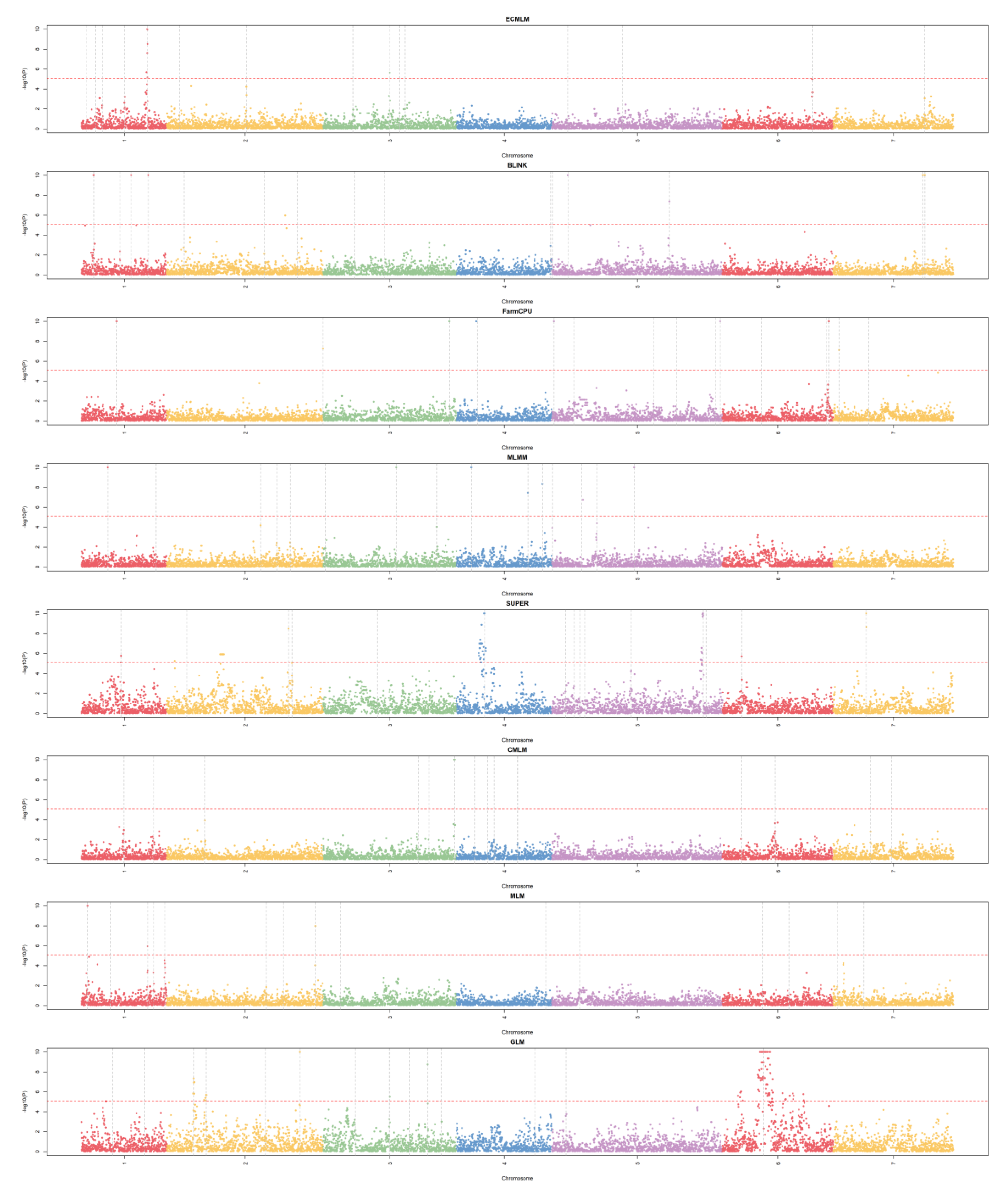
Figure 5.
Bar graph of computational times for eight GWAS methods using a simulated dataset from the World Barley Core Collection (WBCC) with 6,332 SNPs, 318 samples, h² = 0.7, and 15 QTNs across 30 replicates. Bars represent mean runtimes (in seconds) with error bars showing standard deviations, and mean separation letters (a–e) are assigned by Tukey’s HSD test (p = 1.62 × 10⁻¹³⁷).
Disclaimer/Publisher’s Note: The statements, opinions and data contained in all publications are solely those of the individual author(s) and contributor(s) and not of MDPI and/or the editor(s). MDPI and/or the editor(s) disclaim responsibility for any injury to people or property resulting from any ideas, methods, instructions or products referred to in the content. |
© 2025 by the authors. Licensee MDPI, Basel, Switzerland. This article is an open access article distributed under the terms and conditions of the Creative Commons Attribution (CC BY) license (http://creativecommons.org/licenses/by/4.0/).
Copyright: This open access article is published under a Creative Commons CC BY 4.0 license, which permit the free download, distribution, and reuse, provided that the author and preprint are cited in any reuse.


