
Submitted:
30 April 2025
Posted:
30 April 2025
You are already at the latest version
Abstract
Genomic selection (GS) enhances plant breeding by predicting complex traits using genome-wide markers, yet optimal single nucleotide polymorphism (SNP) selection strategies remain unclear. In barley, where polygenic traits arise from numerous small-effect loci, selecting informative SNPs is critical for achieving accurate, stable, and biological relevance. Biological relevance refers to selecting markers that are strongly associated with traits and overlap with causal variants, which simulate functionally important loci contributing to trait variation. We compared four SNP selection methods: standard GS with ridge regression best linear unbiased prediction (rrBLUP), GWAS-Assisted GS, stability-informed selection via the GWAS Stability Index (GSI-GS), and minor allele frequency-based selection (MAF-GS). The study used 318 barley accessions genotyped with 3,974 SNPs and simulated a polygenic trait with a heritability of 0.8. Performance was evaluated across 15 independent 80:20 train-test splits, assessing prediction accuracy (R²), stability (coefficient of variation of R², CV_R²), and biological informativeness. GWAS-Assisted GS achieved the highest prediction accuracy (R² = 0.526), closely followed by GSI-GS (R² = 0.514, p = 0.54). However, GSI-GS showed the greatest prediction stability (CV_R² = 0.165) compared to GS (0.185), GWAS-Assisted GS (0.203), and MAF-GS (0.279), and achieved the lowest root mean square error (16.847). GSI-GS also selected SNPs with stronger trait associations and greater overlap with functional loci than MAF-GS (R² = 0.341). Its SNP selection was largely independent of minor allele frequency (r = 0.008, p = 0.27), supporting robust marker performance across different allele classes. These findings establish GSI-GS as an effective strategy for balancing predictive performance, model stability, and biological relevance in GS pipelines for barley.
Keywords:
bootstrap resampling
; complex traits
; minor allele frequency
; plant breeding
; prediction accuracy
1. Introduction
Selecting the most informative Single Nucleotide Polymorphisms (SNPs) is critical for enhancing the effectiveness of Genomic Selection (GS) in barley (Hordeum vulgare L.) breeding. GS has revolutionized crop improvement by enabling early predictions of complex traits such as yield, disease resistance, and quality, but its success depends heavily on the informativeness and consistency of the selected SNPs. Unlike traditional Marker-Assisted Selection (MAS), which targets specific loci, GS uses genome-wide markers to estimate genomic estimated breeding values without needing prior knowledge of trait-marker associations (Meuwissen et al., 2001; Crossa et al., 2017). In polygenic crops like barley, where traits are influenced by numerous small-effect loci and strong environmental interactions, optimizing SNP selection is critical not only for improving prediction accuracy but also for ensuring the robustness of GS models across environments.
Several SNP selection strategies have been explored to improve the efficiency and interpretability of GS models. Standard GS approaches, such as Ridge Regression Best Linear Unbiased Prediction (rrBLUP), typically use all available genome-wide markers to capture additive genetic variation (Endelman, 2011; Heffner et al., 2009). Although this method maximizes genome coverage, it can be computationally demanding and may dilute model interpretability and predictive precision by including non-informative SNPs. To refine marker sets, Genome-Wide Association Studies (GWAS) have been incorporated into GS pipelines (GWAS-GS), prioritizing SNPs with strong statistical associations to the trait of interest (Bernardo, 2014; Chen et al., 2023).
Alternative methods include minor allele frequency (MAF)-based selection, which prioritizes common alleles but often lacks trait specificity and may overlook important functional loci (Hemstrom et al., 2024). More recently, stability-based approaches such as the GWAS Stability Index (GSI) have emerged, selecting SNPs that are consistently significant across bootstrap GWAS runs to improve reliability (Wang et al., 2014).
Despite these developments, a critical knowledge gap remains in systematically comparing SNP selection strategies in terms of prediction accuracy, model stability, and biological informativeness. While GWAS-Assisted GS can improve accuracy, it may yield unstable markers that reduce reproducibility across populations or environments (Norman et al., 2018). MAF-based filtering, although simple, may sacrifice predictive utility. GSI-based selection offers theoretical advantages in consistency but has not been comprehensively evaluated against GWAS- or MAF-based strategies under realistic trait architectures.
To address this gap, we conducted a comparative evaluation of four SNP selection methods using 318 barley accessions genotyped with 3,974 SNPs and one simulated polygenic trait with heritability of 0.8. The tested models included standard GS using rrBLUP, GWAS-Assisted GS, GSI-GS (bootstrap-based stability filtering), and MAF-GS. Model performance was assessed across 15 independent train-test splits using metrics for prediction accuracy (R²), stability (CV_R²), and biological informativeness. The latter was evaluated through GWAS p-values and overlap with simulated causal variants representing functionally important loci. By integrating accuracy, consistency, and trait relevance, this study provides a practical framework for SNP selection and contributes to optimizing genomic selection pipelines for complex traits in barley.
2. Materials and Methods
2.1. Genotypic Data and Preprocessing
Genotypic data were obtained from 318 barley accessions in the World Barley Core Collection. Accessions were genotyped using the Illumina Infinium iSelect 9K SNP array and aligned to the Morex v3 reference genome (Mascher et al., 2021). The raw dataset, accessed through the Triticeae Toolbox (https://triticeaetoolbox.org/barley), initially included 9,000 SNPs.
Quality control steps excluded SNPs with more than 10% missing data and accessions with more than 30% missing SNPs. SNPs with a MAF below 5% were also removed, resulting in 6,332 SNPs. Taxa names were standardized by removing special characters and assigning unique identifiers for duplicates. Non-numeric SNP columns were converted to numeric, and columns with more than 50% missing values were discarded.
Following alignment between the genotype matrix and SNP map, the final dataset comprised 3,974 high-quality SNPs. Missing genotypes were imputed with column means. SNP values were then standardized to have a mean of zero and a standard deviation of one, to ensure equal weighting of all markers in genomic prediction models and avoid bias from SNPs with larger variances (Gao et al., 2024).
2.2. Phenotype Simulation
A polygenic trait was simulated by randomly selecting 50 causal SNPs, with effect sizes drawn from a standard normal distribution N (0,1), to evaluate GS models under controlled conditions. Phenotypic values were the sum of genetic effects and environmental noise. A broad-sense heritability (h2) of 0.8 was assumed, consistent with complex traits in barley (Gao et al., 2024). Environmental variance was computed using the formula: VarE = VarG×(1−ℎ2) /ℎ2 where VarG is the genetic variance (Falconer and Mackay, 1996). Environmental noise was sampled from a normal distribution with mean zero and standard deviation equal to the square root of VarE. Model performance was evaluated using 15 independent 80:20 train-test splits for the simulated trait.
2.3. Genomic Prediction Models
We evaluated four GS models, each using a different SNP selection strategy. Standard GS estimated marker effects with rrBLUP (Endelman, 2011), using all available SNPs. Marker effects were estimated by restricted maximum likelihood with variance bounds between 10-6 and 1012. Predicted phenotypic values for the test sets were generated, and prediction accuracy was calculated as the squared Pearson correlation (R²) between observed and predicted phenotypes.
GWAS-Assisted GS selected SNPs based on GWAS p-values (p < 0.01) calculated on the training set, using the BLINK model implemented in GAPIT (Lipka et al., 2012; Tang et al., 2016; Wang et al., 2021). Unlike classical marker-assisted selection (MAS), which directly targets major-effect loci, GWAS-Assisted GS incorporates selected SNPs into a whole-genome prediction model. To reflect this distinction and avoid conceptual confusion, we consistently refer to this approach as GWAS-Assisted GS.
GSI-GS selected SNPs based on the GSI, calculated from 50 bootstrap GWAS runs in which training samples were resampled with replacement. In each bootstrap run, SNPs significant at p < 0.01 were recorded, and GSI values were computed as the proportion of runs in which each SNP was significant. SNPs with GSI ≥ 0.15 were selected; if fewer than 50 SNPs met this threshold, the top 50 SNPs by GSI were retained. The threshold of 0.15 was chosen to balance marker stability with marker quantity based on preliminary simulations.
MAF-GS selected the top N SNPs by highest MAF, where N matched the number of GSI-selected SNPs for each phenotype-split combination. The stability of MAF-selected SNPs was assessed using the same bootstrap GWAS results for a consistent comparison across methods.
2.4. Evaluation Metrics
Model performance was evaluated based on prediction accuracy (R²), calculated as the squared Pearson correlation between observed and predicted values in the 20% held-out test set for each split. Additional evaluation metrics included root mean square error (RMSE) and prediction consistency (CV_R2, the coefficient of variation of R² across splits). Biological relevance used -log₁₀(P-values) from GWAS on the train-test split. These values are compared to GSI- and MAF-selected SNPs. Functional relevance involved 397 simulated functional SNPs. These represented causal loci. Overlaps with selected SNPs were counted. Higher overlaps indicate greater alignment with biologically important markers. This enhances interpretability for barley breeding.
2.5. Statistical Analysis and Visualization
Performance metrics were averaged across 15 train-split combinations. Standard errors (SE) were calculated as the standard deviation divided by the square root of the number of splits. Paired t-tests compared R² values the models to evaluate statistical significance. The relationship between GSI stability and MAF was evaluated using Pearson correlation. To further examine how stability varies across allele frequencies, GSI-selected SNPs were grouped into MAF bins: 0–0.1, 0.1–0.2, 0.2–0.3, 0.3–0.4, and 0.4–0.5. For each bin, GSI stability and its standard error were calculated across all splits. These equal-width intervals ensured a uniform assessment across the full MAF spectrum and reduced bias toward specific frequency ranges.
Visualization outputs included a summary table of R², RMSE, and CV_R²; a bar plot comparing prediction accuracies; and a scatter plot of GSI stability versus MAF. All analyses were performed in R version 4.3.1 (R Core Team, 2023) using the following packages: data.table (Dowle and Srinivasan, 2023), caret (Kuhn, 2023), rrBLUP (Endelman, 2011), GAPIT (Lipka et al., 2012; Tang et al., 2016; Wang et al., 2021), MASS (Venables and Ripley, 2002), ggplot2 (Wickham, 2016), pheatmap (Kolde, 2019), cowplot (Wilke, 2020), and dplyr (Wickham et al., 2023).
3. Results
3.1. Prediction Accuracy
Model performance was evaluated across 15 independent 80:20 train-test splits using a simulated polygenic trait. Table 1 summarizes the mean R², RMSE, and CV_R² values with associated standard errors (SE).
Among the models, GWAS-Assisted GS achieved the highest mean R² (0.526 ± 0.028), comparable to GSI-GS (0.514 ± 0.022). Standard GS using rrBLUP and MAF-GS showed lower accuracies (0.483 ± 0.023 and 0.341 ± 0.025, respectively). GSI-GS achieved the lowest RMSE (16.847 ± 0.145), outperforming GWAS-Assisted GS (17.003 ± 0.187), GS (16.988 ± 0.208), and MAF-GS (17.408 ± 0.242).
Paired t-tests revealed that GWAS-Assisted GS (p = 3.96e-07), GSI-GS (p = 7.79e-06), and GS (p =1.04e-07) significantly outperformed MAF-GS. No significant differences were observed between GWAS-Assisted GS and GSI-GS (p = 0.545), or between either method and GS (p = 0.06 and 0.13).
Figure 1.
Prediction Accuracy Across Models.
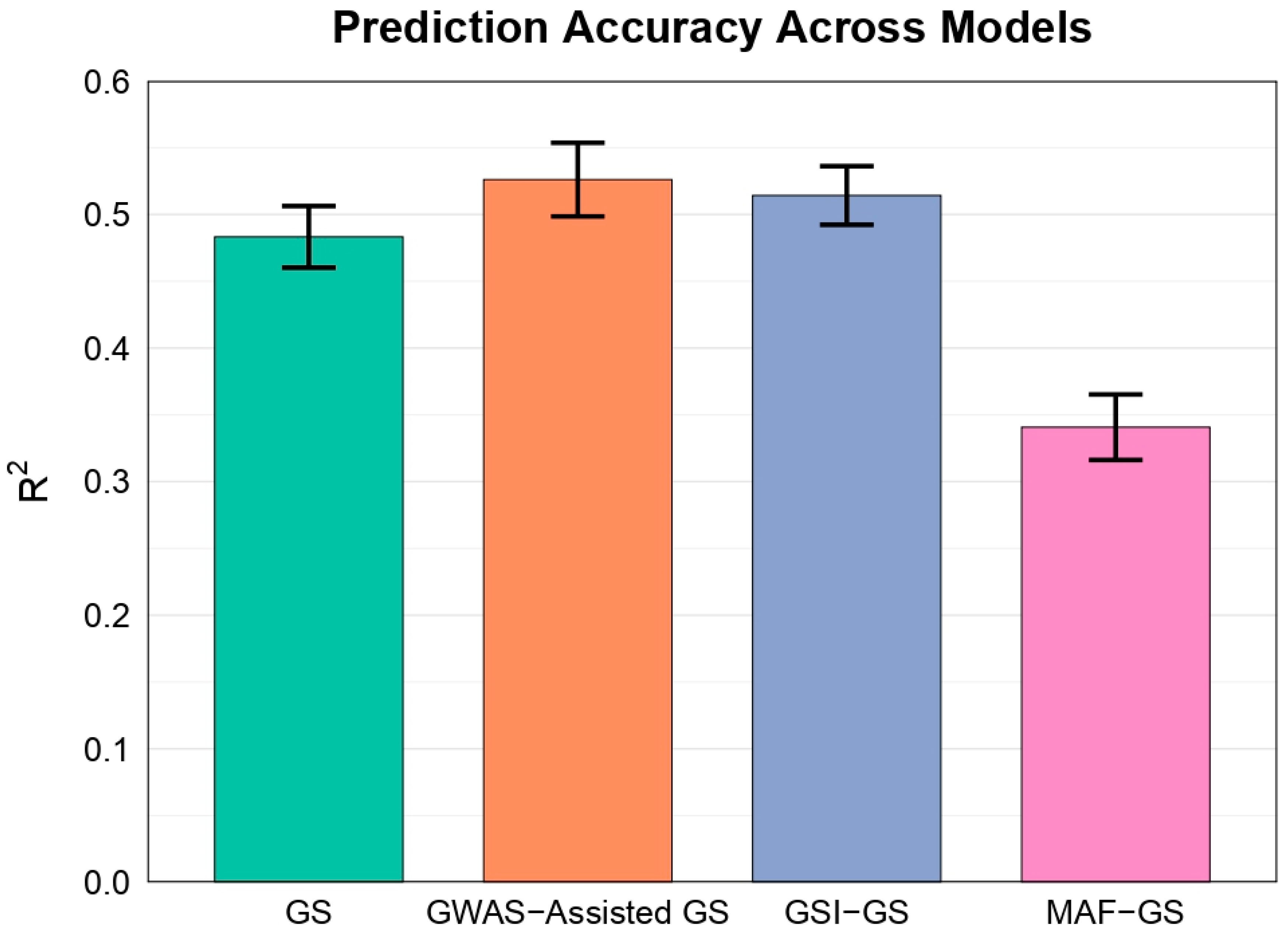
Bar plot showing mean R² values (± standard error) for four GS models across 15 train-test splits of one polygenic trait. GS uses all SNPs with ridge regression; GWAS-Assisted GS selects SNPs via GWAS p-values; GSI-GS selects SNPs using GSI from bootstrap GWAS for stability; MAF-GS selects SNPs by highest MAF.
Summary of genomic prediction model performance across 15 train-test splits of one polygenic trait. R² denotes the squared Pearson correlation between observed and predicted values; RMSE is the root mean squared error; CV_R2 represents the coefficient of variation of R² values across splits. SE is the standard error. Models include standard genomic selection (GS), GWAS-Assisted GS, GSI-GS, and MAF-GS.
3.2. Model Stability and Consistency
Prediction consistency, measured by CV_R², was highest for GSI-GS (0.165), followed by GS (0.185), GWAS-Assisted GS (0.203), and MAF-GS (0.279) (Table 1).
Analysis of GSI stability versus MAF revealed a weak, non-significant correlation (r = 0.0082, p = 0.2766), suggesting that GSI-selected SNPs are stable across different MAF ranges. Stability was highest in the 0.2–0.3 MAF range (0.0566 ± 0.00127), followed by 0.3–0.4 (0.0459 ± 0.00073), 0.4–0.5 (0.0441 ± 0.00083), 0.1–0.2 (0.0412 ± 0.00073), and 0–0.1 (0.0347 ± 0.00122). Figure 2 shows that stable SNPs often had moderate allele frequencies, highlighting GSI’s robustness. These findings support GSI-GS’s advantage in selecting consistently informative SNPs, leading to reliable genomic predictions.
Scatter plot of GSI stability versus MAF, showing the proportion of bootstrap runs (out of 50) where SNPs were significant (p < 0.01) across 15 train-test splits of one polygenic trait. A weak, non-significant correlation is observed (r = 0.0082, p = 0.2766), indicating stable SNPs often have moderate MAF (0.2–0.3). GSI stability reflects GSI-GS’s SNP selection approach, emphasizing consistency across bootstrap runs.
3.3. Trait Association and Functional Relevance
Trait association strength, based on –log₁₀ (GWAS p-values) from the train-test split, was higher for GSI-GS (1.25) than MAF-GS (0.42), with the difference being statistically significant (p < 0.01).
Biological relevance was further assessed by simulating 397 functional SNPs (10% of all markers) to represent causal loci. Standard GS, using all markers, captured all 397. GWAS-Assisted GS captured 62, GSI-GS captured 27, and MAF-GS only 3. These overlap counts indicate the extent to which each SNP selection strategy captures biologically relevant markers, with higher overlaps reflecting greater alignment with functional loci critical for trait expression.
4. Discussion
4.1. Prediction Accuracy in Genomic Selection
Incorporating GWAS-derived SNPs into GS models often enhances prediction accuracy for complex traits in crops, as shown in prior studies (Norman et al., 2018). Our findings support this trend, with GWAS-Assisted GS achieving the highest prediction accuracy (R² = 0.526 ± 0.028), closely followed by GSI-GS (R² = 0.514 ± 0.022, p = 0.5454). In contrast, standard GS (R² = 0.483 ± 0.023) and MAF-GS (R² = 0.341 ± 0.025) performed less effectively (Figure 1). This demonstrates that pre-selecting trait-associated SNPs improves GS performance relative to using all SNPs or filtering by allele frequency (Chen et al., 2023). Notably, GSI-GS’s comparable accuracy, combined with superior stability and lower RMSE (16.847 ± 0.145), positions it as a promising strategy for GS in barley breeding programs targeting polygenic traits.
4.2. Stability and Consistency of Genomic Predictions
Model consistency is critical for reliable GS application across varying populations and environments (Jannink et al., 2010). GSI-GS exhibited the greatest stability, with the lowest CV_R2 (0.165), outperforming GWAS-Assisted GS (0.203), GS (0.185), and MAF-GS (0.279) (Table 1). This advantage stems from the GSI’s bootstrap framework, which uses bootstrapped GWAS to minimize sampling noise and prioritize reproducible associations (Wang et al., 2014). In contrast, GWAS-Assisted GS relies on all SNPs and GS and MAF-GS apply broader or less informative selection, reducing consistency. These findings highlight GSI-GS’s strength in enhancing the robustness of genomic predictions for breeding applications.
4.3. Biological Relevance of SNP Selection
Biologically informative SNP selection strengthens the interpretability and utility of GS models in crop improvement (Bernardo, 2014). Stability-informed selection via GSI-GS and GWAS-assisted selection outperformed frequency-based selection (MAF-GS) in capturing biologically relevant SNPs. GSI-GS achieved stronger trait associations, with a mean -log₁₀(P-value) of 1.25 versus 0.42 for MAF-GS (p < 0.01). Among selective methods, GWAS-assisted selection identified 62 functional SNPs, followed by GSI-GS with 27, while MAF-GS detected only 3. Standard genomic selection captured all 397 functional SNPs due to its non-selective approach but lacks prioritization for interpretability.
GWAS-assisted selection’s broader overlap suggests it captures more biologically important loci. However, GSI-GS prioritizes stable SNPs with consistent trait associations, aligning with findings on stable markers’ value (Spindel et al., 2015). GSI-GS’s lower overlap (27 vs. 62) reflects a trade-off for enhanced reliability across splits. This balance suits breeding programs targeting polygenic traits. MAF-GS’s minimal overlaps stem from its bias toward high-frequency SNPs, limiting biological relevance. GSI-GS offers a practical compromise, improving interpretability over non-selective or frequency-based methods while maintaining accuracy and stability for trait-targeted breeding.
4.4. Advantages of GSI-Based Selection Across MAF Ranges
A persistent challenge in GS is identifying informative SNPs across the allele frequency spectrum. Frequency-based filtering often prioritizes common variants, potentially overlooking rare but important loci (Zhu et al., 2017; Li and Leal, 2008). In this analysis, GSI-GS showed minimal dependence on MAF (r = 0.0082, p = 0.2766), selecting stable markers across a wide frequency range, with peak stability observed in the 0.2–0.3 bin (0.0566 ± 0.0013) (Figure 2). In contrast, MAF-GS was biased toward high-MAF SNPs, while GS and GWAS-Assisted GS lacked specificity or stability (Crossa et al., 2017). These results demonstrate that GSI-GS balances allele frequency representation, enabling both predictive accuracy and maintaining genetic diversity is critical for durable trait improvement in breeding programs.
4.5. Limitations and Future Directions
Despite its strengths, this study relied on simulated traits, limiting generalizability to real-world environments and broader germplasm pools. Genotype-by-environment interactions, in particular, remain unaddressed. Future work should validate GSI-GS in multi-environment field trials and explore its integration with known QTLs or functional annotations to refine SNP prioritization. Expanding the application of GSI-based selection to other species and trait architectures will further clarify its utility in building robust, biologically informed GS pipelines for sustainable crop improvement.
5. Conclusion
This study presents a comprehensive evaluation of SNP selection strategies for genomic selection in barley, emphasizing prediction accuracy, model stability, and biological informativeness. Among the four approaches tested, GSI-GS emerged as the most robust, offering a strong balance between predictive performance (second only to GWAS-Assisted GS), consistency across data splits, and alignment with functionally important loci. By incorporating SNP stability through the GSI, this method enables reproducible and efficient marker selection for polygenic trait prediction. These findings address key limitations in existing SNP selection methods and provide practical guidance for advancing genomic selection pipelines. Future work should focus on validating GSI-GS using real-world phenotypic data across diverse environments, and on integrating it with functional annotations and known QTLs to enhance its applicability. Collectively, this work supports more informed and stable SNP prioritization, helping accelerate the development of high-performing, resilient barley cultivars to meet global food security needs.
Acknowledgement
The authors gratefully acknowledge Dr. Zhiwu Zhang, instructor of Statistical Genomics, for his guidance and expertise in designing and overseeing this course. They also sincerely thank the Teaching Assistant, Meijing Liang, for her support, detailed feedback, and assistance in resolving technical challenges during this assignment
References
- Bernardo, R. (2014). Genomewide selection when major genes are known. Crop Science, 54(1), 68–75. [CrossRef]
- Chen, Z.-Q., Klingberg, A., Hallingbäck, H. R., & Wu, H. X. (2023). Preselection of QTL markers enhances accuracy of genomic selection in Norway spruce. BMC Genomics, 24(1), 147. [CrossRef]
- Crossa, J., Pérez-Rodríguez, P., Cuevas, J., Montesinos-López, O., Jarquín, D., de los Campos, G., Burgueño, J., González-Camacho, J. M., Pérez-Elizalde, S., Beyene, Y., Dreisigacker, S., Singh, R., Zhang, X., Gowda, M., Roorkiwal, M., Rutkoski, J., & Varshney, R. K. (2017). Genomic selection in plant breeding: Methods, models, and perspectives. Trends in Plant Science, 22(11), 961–975. [CrossRef]
- Dowle, M., & Srinivasan, A. (2019). data. table: Extension of ‘data. frame’. R package version 1.12.8. Computer Software. Retrieved from https://CRAN. R-project. org/package= data.table.
- Endelman, J. B. (2011). Ridge regression and other kernels for genomic selection with R package rrBLUP. The Plant Genome, 4(3), 250–255. [CrossRef]
- Falconer, D. S., & Mackay, T. F. C. (1996). Introduction to Quantitative Genetics (4th ed.). Longman.
- Gao, Y., Stein, M., Oshana, L., Zhao, W., Matsubara, S., & Stich, B. (2024). Exploring natural genetic variation in photosynthesis-related traits of barley in the field. Journal of Experimental Botany, 75(16), 4904–4925. [CrossRef]
- Heffner, E. L., Sorrells, M. E., & Jannink, J.-L. (2009). Genomic selection for crop improvement. Crop Science, 49(1), 1–12. [CrossRef]
- Hemstrom, W., Grummer, J. A., Luikart, G., & Christie, M. R. (2024). Next-generation data filtering in the genomics era. Nature Reviews Genetics, 25(11), 750–767. [CrossRef]
- Jannink, J.-L., Lorenz, A. J., & Iwata, H. (2010). Genomic selection in plant breeding: From theory to practice. Briefings in Functional Genomics, 9(2), 166–177. [CrossRef]
- Kolde, R. (2019). pheatmap: Pretty Heatmaps. R package version 1.0.12. https://CRAN.R-project.org/package=pheatmap.
- Kuhn, M. (2022). caret: Classification and Regression Training. R package version 6.0-94. https://CRAN.R-project.org/package=caret.
- Lipka, A. E., Tian, F., Wang, Q., Peiffer, J., Li, M., Bradbury, P. J., Gore, M. A., Buckler, E. S., & Zhang, Z. (2012). GAPIT: Genome association and prediction integrated tool. Bioinformatics, 28(18), 2397–2399. [CrossRef]
- Li, B., & Leal, S. M. (2008). Methods for detecting associations with rare variants for common diseases: Application to analysis of sequence data. American Journal of Human Genetics, 83(3), 311–321. [CrossRef]
- Mascher, M., Wicker, T., Jenkins, J., Plott, C., Lux, T., Koh, C. S., Ens, J., Gundlach, H., Boston, L. B., Tulpová, Z., Holden, S., Hernández-Pinzón, I., Scholz, U., Mayer, K. F. X., Spannagl, M., Pozniak, C. J., Sharpe, A. G., Šimková, H., Moscou, M. J., … Stein, N. (2021). Long-read sequence assembly: A technical evaluation in barley. The Plant Cell, 33(6), 1888–1906. [CrossRef]
- Meuwissen, T. H. E., Hayes, B. J., & Goddard, M. E. (2001). Prediction of total genetic value using genome-wide dense marker maps. Genetics, 157(4), 1819–1829. [CrossRef]
- Norman, A., Taylor, J., Edwards, J., & Kuchel, H. (2018). Optimising genomic selection in wheat: effect of marker density, population size and population structure on prediction accuracy. G3: Genes, Genomes, Genetics, 8(9), 2889-2899.
- Panagiotou, O. A., Evangelou, E., & Ioannidis, J. P. A. (2010). Genome-wide significant associations for variants with minor allele frequency of 5% or less—An Overview: A HuGE Review. American Journal of Epidemiology, 172(8), 869–889.
- Pongpanich, M., Sullivan, P. F., & Tzeng, J.-Y. (2010). A quality control algorithm for filtering SNPs in genome-wide association studies. Bioinformatics, 26(14), 1731–1737. [CrossRef]
- R Core Team. (2023). R: A Language and Environment for Statistical Computing. R Foundation for Statistical Computing. https://www.R-project.org/.
- Spindel, J., Begum, H., Akdemir, D., Virk, P., Collard, B., Redoña, E., et al. (2015). Genomic selection and association mapping in rice (Oryza sativa): effect of trait genetic architecture, training population composition, marker number and statistical model on accuracy of rice genomic selection in elite, tropical rice breeding lines. PLoS Genetics, 11(2), e1004982. [CrossRef]
- Tang, Y., Liu, X., Wang, J., Li, M., Chen, Q., Xie, F., Zhang, Z., & Zhang, G. (2016). GAPIT Version 3: An interactive analytical tool for genomic association and prediction. The Plant Genome, 9(3), 1–12. [CrossRef]
- Venables, W. N., & Ripley, B. D. (2002). Modern Applied Statistics with S (4th ed.). Springer. [CrossRef]
- Wang, Q., Tian, F., Pan, Y., Buckler, E. S., & Zhang, Z. (2014). A SUPER Powerful Method for Genome Wide Association Study. PLOS ONE, 9(9), e107684. [CrossRef]
- Wang, J., & Zhang, Z. (2021). GAPIT Version 3: Boosting Power and Accuracy for Genomic Association and Prediction. Genomics, Proteomics & Bioinformatics, 19(4), 629–640. [CrossRef]
- Wickham, H. (2016). ggplot2: Elegant Graphics for Data Analysis (2nd ed.). Springer. [CrossRef]
- Wilke, C. O. (2024). cowplot: Streamlined Plot Theme and Plot Annotations for “ggplot2” (Version 1.1.3) [Computer software].
Figure 2.
GSI Stability vs. MAF.
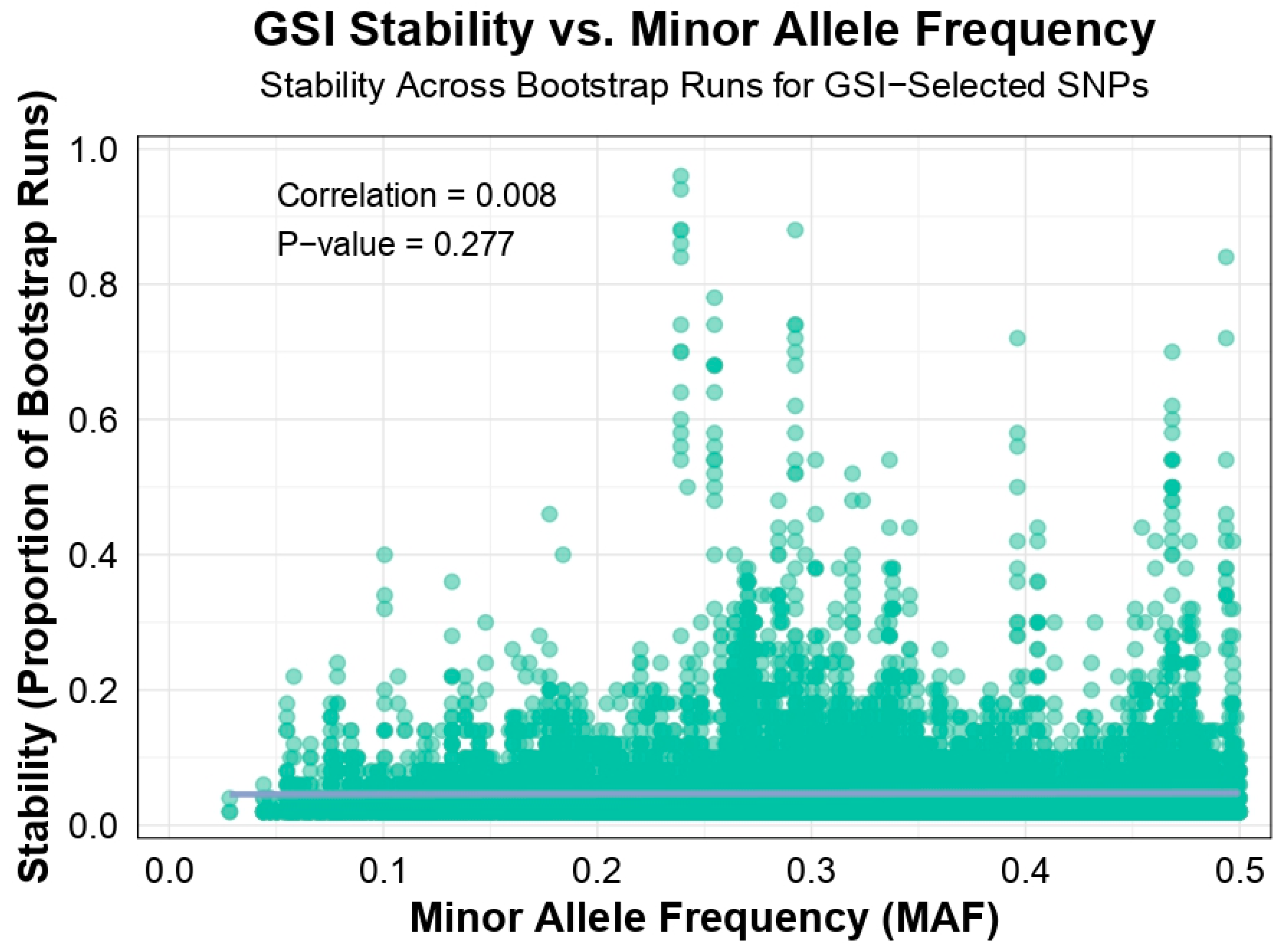

Table 1.
Summary Statistics of Model Performance.
| Model | R² ± SE | RMSE ± SE | CV_R2 |
|---|---|---|---|
| GS (rrBLUP) | 0.483 ± 0.023 | 16.988 ± 0.208 | 0.185 |
| GWAS-Assisted GS | 0.526 ± 0.028 | 17.003 ± 0.187 | 0.203 |
| GSI-GS | 0.514 ± 0.022 | 16.847 ± 0.145 | 0.165 |
| MAF-GS | 0.341 ± 0.025 | 17.408 ± 0.242 | 0.279 |
Disclaimer/Publisher’s Note: The statements, opinions and data contained in all publications are solely those of the individual author(s) and contributor(s) and not of MDPI and/or the editor(s). MDPI and/or the editor(s) disclaim responsibility for any injury to people or property resulting from any ideas, methods, instructions or products referred to in the content. |
© 2025 by the authors. Licensee MDPI, Basel, Switzerland. This article is an open access article distributed under the terms and conditions of the Creative Commons Attribution (CC BY) license (http://creativecommons.org/licenses/by/4.0/).
Copyright: This open access article is published under a Creative Commons CC BY 4.0 license, which permit the free download, distribution, and reuse, provided that the author and preprint are cited in any reuse.


