Evaluating GWAS Model Performance Across Heritability and Polygenicity Gradients in Simulated Plant Trait Data

Nosheen Fatima

doi:10.20944/preprints202503.2269.v1

Submitted:

30 March 2025

Posted:

31 March 2025

You are already at the latest version

Abstract

Genome-wide association studies (GWAS) are a widely applied approach for dissecting complex traits in crops. In this study, we systematically compared the performance of eight GWAS models across a range of heritability levels (0.3–0.8), followed by deeper analysis of the top three models—BLINK, FarmCPU, and MLMM—under two polygenic scenarios involving 50 and 100 quantitative trait loci (QTLs). Our results highlight the importance of trait heritability and genetic architecture in determining GWAS model effectiveness. BLINK consistently detected the highest number of true positives (TPs), particularly for moderately heritable traits, while MLMM showed superior mapping resolution. These findings provide practical guidance for selecting appropriate GWAS methods based on trait complexity.

Keywords:

Genome-wide association study (GWAS)

;

heritability

;

polygenic traits

;

mapping resolution

;

true positives

;

multi-locus models

;

BLINK

;

FarmCPU

;

MLMM

;

quantitative trait loci (QTL)

Subject:

Biology and Life Sciences - Agricultural Science and Agronomy

Introduction

In plant research, two primary strategies have been commonly used to understand how genetic differences relate to physical traits: linkage mapping (also known as QTL mapping) and association mapping (or linkage disequilibrium mapping) (Xu et al., 2017). QTL mapping has been instrumental in pinpointing many genetic regions over the years. However, it relies on biparental populations, which limits the number of recombination events and genetic diversity available. As a result, it often falls short in resolution and scope—especially when dealing with complex traits influenced by many genes with small effects. For instance, QTL mapping struggled to provide high-resolution insights into resistance to Fusarium ear rot in maize (Wu et al., 2020). On top of that, the maize genome is over 85% repetitive, which makes it even harder to use traditional linkage methods for fine mapping (Xiao et al., 2017).

On the other hand, genome-wide association studies (GWAS) tap into the natural genetic variation found in diverse plant populations and use recombination events that have built up over many generations. This gives GWAS an edge in terms of mapping resolution and the ability to detect a broader range of alleles compared to QTL mapping (Carlson et al., 2019; Alqudah et al., 2020). GWAS has been widely used to identify genetic regions linked to traits like flowering time, yield, nutritional content, and stress tolerance in crops such as maize, wheat, and rice. However, its effectiveness depends on several factors—like how much variation there is in the trait, its heritability, the size and structure of the population being studied, and patterns of linkage disequilibrium (IJMS, 2023). Low heritability or inconsistent trait measurements can weaken the results. Also, if population structure isn’t properly accounted for, it can lead to false positives. The rate at which LD breaks down also affects how many genetic markers are needed and how precise the mapping can be. To boost accuracy and reduce false discoveries, newer GWAS methods now often use kinship matrices, principal component analysis (PCA) for population correction, and advanced multi-locus models like MLMM, FarmCPU, and BLINK.

GWAS models fall into two main categories: single-locus and multi-locus approaches, each with its own strengths depending on the research focus. The General Linear Model (GLM) was one of the earliest GWAS methods, correcting for population structure via PCA or Q-matrix analysis (Price et al., 2006). However, it fails to account for familial relatedness, which can lead to inflated p-values. The Mixed Linear Model (MLM) addresses this by incorporating a kinship matrix (K) to account for relatedness (Yu et al., 2006), reducing false positives but sometimes being overly conservative.To improve computational efficiency, Compressed MLM (CMLM) groups individuals into clusters while maintaining accuracy (Zhang et al., 2010). SUPER refines MLM by using a subset of associated markers to define kinship, enhancing statistical power (Wang et al., 2014). The Multi-Locus Mixed Model (MLMM) includes multiple loci in a stepwise fashion, effectively capturing polygenic effects and reducing false positives (Segura et al., 2012). FarmCPU improves upon MLMM by separating fixed and random effects to reduce confounding and boost both power and computational efficiency (Liu et al., 2016).

Finally, BLINK eliminates the random effect component entirely, using Bayesian Information Criteria (BIC) for model selection. This fixed-effect-only approach enhances both speed and power, making it highly efficient for large-scale GWAS (Huang et al., 2019).ng that’s less demanding on computing resources. But when it comes to digging into the genetic details of complex traits, multi-locus models offer much greater power and precision. That’s why they’ve become key tools in today’s plant and animal breeding research. Table 1 provides a summary of these models.

This distinction between single-locus and multi-locus becomes particularly important when dealing with polygenic traits—those influenced by many genes, each with a small effect. Traits like grain yield, disease resistance, drought tolerance, and other key performance indicators fall in this category and are critical for crop breeding programs. Deconstructing the genetics of such traits requires statistical models that are not only powerful but also capable of maintaining high resolution even when the genetic signals are faint and spread out. Unlike the situation with traits controlled by a few major genes, polygenic traits need models that can capture the combined influence of many genes with small effects, even when gene effects per se are weak or the alleles linked to them are rare. As agriculture seeks to improve both yield and climate resilience, precise tools are necessary to uncover the genetic underpinnings of these traits—tools that can inform more effective marker-assisted selection and genomic prediction.

In this study, we conducted a comprehensive simulation-based model comparison of GWAS performance across a range of trait complexities. First, we compared eight GWAS models across a range of heritabilities (0.3 to 0.8) using traits controlled by a fixed number of QTLs. Building on these results, we compared model performance along a gradient of polygenicity, simulating phenotypes controlled by 50 and 100 QTLs at a constant heritability (h² = 0.5). In addition to classical power evaluations, we also addressed mapping resolution by measuring the distance of significant markers from their underlying causal variants. This dual focus on detection and localization provides a more complete view of model behavior, especially under conditions of realistic trait architectures. The findings of this study will inform future GWAS-based complex trait dissection in crops, with relevance to both research and breeding.

Materials and Methods

Genotypic Data

Raw SNP data in HapMap format were obtained from the Maize HapMap project (Panzea Database; https://www.panzea.org). These data comprise genome-wide polymorphisms from the Maize Diversity Panel, including the Nested Association Mapping (NAM) population and inbred association lines. Comprehensive quality control was performed on the raw HapMap SNP dataset to ensure reliable downstream analysis. First, SNPs with high levels of missing data were removed by calculating the proportion of missing genotypes for each SNP and applying a cutoff of no more than 20% missingness. To filter out rare variants, a minor allele frequency (MAF) threshold was applied—retaining only those SNPs with a MAF of at least 0.05, based on the lowest observed allele frequency across the population. Following filtering, GAPIT with default settings was used to impute remaining missing genotypes. For improved computational efficiency during model comparisons, SNPs labeled as "chromosome 0," which typically represent unlinked markers, were excluded. This process resulted in a curated set of 28,921 high-quality SNPs. Although chromosome 0 SNPs were excluded in this analysis for practical reasons, it is recommended to retain these markers in standard GWAS pipelines, as they may capture biologically meaningful associations in broader population studies. To account for population structure in the genotypic data prior to phenotypic simulation, Principal Components Analysis (PCA) was conducted using the prcomp function in R (R Core Team, 2022) and iteratively within GWAS analyses through the GAPIT3 package (Wang and Zhang, 2021). It showed the 25 founder lines which is in accordance to the population structure of this panel.

Phenotypic Simulation

Phenotypic data (Y) were generated from the reduced genotypic dataset using a custom R script. Two uncorrelated quantitative traits were simulated, each across a range of heritability values from h² = 0.3 to 0.8. For each trait, 20 quantitative trait loci (QTLs) were randomly selected across the genome, and the corresponding SNP identifiers were archived for post-GWAS validation. QTL effects (g_j) were sampled from a standard normal distribution (μ = 0, σ² = 1). Phenotypes were modeled using an additive genetic model:

yᵢ = ∑ⱼ₌₁²⁰ gⱼ sᵢⱼ + eᵢ

where y_i is the phenotypic value of the i^th individual, s_ij is the genotype at the j^th QTL for the i^th individual, and e_i is the residual error. Additive genetic values were calculated as the sum of QTL effects weighted by genotypes. Residual variance (V_e) was determined by the relationship V_e = V_g(1 − h²)/h², where V_g is the additive genetic variance. Errors were sampled from a normal distribution (μ = 0, V_e) and added to the genetic values to produce the final phenotype. To model polygenic trait architectures, phenotypic data were also simulated using the GAPIT.Phenotype.Simulation function, specifying 50 and 100 QTLs under moderate heritability (h² = 0.5) using the same genotypic data. This approach mimics complex traits governed by many minor-effect loci, where each QTL contributes only a small proportion to the total phenotypic variance. Effect sizes were randomly assigned to avoid dominance by any single locus. These polygenic simulations were critical for evaluating GWAS model performance under varying levels of polygenicity, only top selected models from heritability study were chosen. Phenotypic quality control (pQC) included outlier detection via histograms, Q-Q plots, and the odetector R package (Cebeci et al., 2022), followed by Shapiro-Wilk tests for normality. No significant outliers were identified, and both traits conformed to normality assumptions (p > 0.05).

Statistical Analysis and Validation

Following GWAS, raw p-values were adjusted to account for multiple testing using both the Bonferroni correction (a conservative approach) and the Benjamini-Hochberg procedure for controlling the false discovery rate (FDR; a less conservative method), applied at significance thresholds of α = 0.05 and α = 0.01. Adjusted p-values were calculated using R’s p.adjust function (R Core Team, 2022), and significant SNPs were identified directly from GAPIT3 outputs.

True positives (TPs) were defined as significant SNPs that matched the simulated quantitative trait loci (QTLs), while unmatched significant SNPs were classified as false positives (FPs). Type I error was characterized by the incorrect identification of non-causal SNPs as significant, and statistical power was measured by the model's ability to detect true causal associations (TPs). All analyses were conducted using R version 4.2.2 on a macOS system (16 GB RAM) with the following tools: GAPIT3 (Wang and Zhang, 2021): for GWAS and kinship matrix estimation and CMplot (Yin, 2022): for generating Manhattan and Q-Q plots.

Results

Genomic Inflation Values

Genomic inflation factor (λGC) is a metric used to assess the extent of systematic bias in genome-wide association studies (GWAS), particularly the inflation of test statistics due to population structure, relatedness, or other confounding factors. A λGC value close to 1.0 indicates well-calibrated test statistics, suggesting that the model effectively controls for confounding. Values significantly greater than 1.0 reflect inflation, implying an excess of false positives, while values below 1.0 suggest deflation, which may lead to missed true associations. Evaluating λGC across different GWAS models provides insight into how well each method manages type I error and controls for population structure. This is particularly important when comparing model performance under varying trait architectures and heritability levels. The results are given in Table 2. It can be seen from the analysis of genomic inflation factors (λGC) across traits with low (h² = 0.3), medium (h² = 0.5), and high (h² = 0.8) heritability revealed consistent patterns in model performance. At low heritability (h² = 0.3), inflation was moderate for the General Linear Model (GLM), with a λGC of 1.292, reflecting limited control of population structure. Mixed linear models such as MLM, CMLM, and ECMLM demonstrated better calibration, with λGC values between 0.968 and 0.986, indicating strong control over false positives. Among multi-locus models, FarmCPU showed good control (λGC = 0.938), while BLINK exhibited slightly elevated inflation (λGC = 1.134). At medium heritability (h² = 0.5), GLM showed substantial inflation (λGC = 3.496), while the MLM-based models remained well-calibrated around 1.001. FarmCPU and BLINK continued to perform reliably, maintaining λGC values of 0.821 and 0.972, respectively, suggesting a strong balance between statistical power and control of type I error. At high heritability (h² = 0.8), GLM remained inflated (λGC = 2.098), while mixed models like MLM, CMLM, and ECMLM consistently held λGC values close to 0.986, demonstrating robustness across trait architectures. FarmCPU again maintained deflation (λGC = 0.870), and BLINK performed slightly better than at lower heritability (λGC = 1.047), showing that both models scale well with increasing genetic signal strength. Overall, the results highlight the limitations of GLM in controlling genomic inflation, particularly as heritability increases. Mixed linear models (MLM, CMLM, ECMLM) consistently maintained λGC values near 1.0 across all heritability levels, confirming their robustness in accounting for confounding effects. Among multi-locus approaches, FarmCPU showed the most stable and conservative inflation profile, while BLINK remained well-calibrated and responsive to higher genetic signal, making both suitable choices for GWAS of complex traits. All analyses were performed using R v4.2.2 on a macOS system, utilizing GAPIT3 for model implementation and output processing. Multiple testing corrections were applied using Bonferroni and Benjamini-Hochberg (FDR) methods at α=0.05 and 0.01, providing a rigorous yet biologically plausible framework for identifying significant associations.

Comparison of GWAS Model Performance Across Heritability and Significance Thresholds

The comparison of GWAS models under Bonferroni and FDR corrections at 1% and 5% significance levels revealed distinct differences in power and false positive control across heritability levels. At low heritability (h² = 0.3), detection power was generally limited. Under Bonferroni correction at α = 0.01, only a few models detected more than 2 true positives (TPs). For instance, BLINK identified 5 TPs with 1 false positive (FP), while FarmCPU detected 4 TPs with 3 FPs. Mixed models like CMLM and ECMLM identified only 2 TPs with 1 FP each, and GLM showed 2–3 TPs depending on the threshold. FDR adjustment at α = 0.05 slightly improved detection, with BLINK reaching 7 TPs (but with 6 FPs), while GLM exhibited higher FP rates (up to 5), indicating reduced specificity. At moderate heritability (h² = 0.5), model performance improved across the board. Under Bonferroni correction, BLINK and FarmCPU achieved 9 and 8 TPs, respectively, with minimal false positives (1–2 FPs). When applying FDR at α = 0.05, both models reached 10 TPs, although BLINK maintained lower FPs (3) compared to FarmCPU (4). Traditional models such as GLM and MLM continued to lag, with GLM producing up to 7 FPs at the higher threshold. At high heritability (h² = 0.8), all models demonstrated stronger detection capabilities. BLINK and FarmCPU reached perfect detection (10 TPs) under Bonferroni correction with only 0–1 FP, clearly outperforming other methods. Under FDR, while sensitivity remained high, false positives increased slightly for all models—GLM reached as many as 10 FPs, whereas BLINK and FarmCPU maintained strong performance with 10 TPs and only 2–3 FPs. These trends are visually illustrated in Figure 1 and Figure 2, which display the number of true positives detected across heritability levels under Bonferroni correction at α = 0.05 and α = 0.01, respectively. As heritability increases, TP counts rise for all models, with BLINK and FarmCPU consistently outperforming others, especially at moderate to high heritability levels. The visual separation among models becomes more distinct from h² ≥ 0.5, reinforcing the numerical trends and highlighting the superior sensitivity of multi-locus approaches under stringent significance thresholds. While Bonferroni correction provided stricter control over false positives, FDR adjustment allowed for increased sensitivity, particularly at moderate and high heritability levels. Under FDR, BLINK and FarmCPU achieved high true positive rates with only a modest increase in false positives. Across both correction methods, BLINK and FarmCPU demonstrated superior performance, offering the best trade-off between statistical power and control of type I error—making them ideal choices for GWAS of complex traits under varying heritability conditions.

Quantile-Quantile (QQ) Plot Analysis

The QQ plots for Trait 1 and Trait 2 illustrate the distribution of observed versus expected p-values under the null hypothesis for each GWAS model, Figure 3. Models with well-calibrated test statistics should follow the diagonal line, indicating no systematic inflation or deflation. For both traits, GLM and SUPER show clear deviations from the expected distribution, especially in the tail region, suggesting inflation of p-values and a higher risk of false positives. In contrast, models like MLM, CMLM, ECMLM, and MLMM remain closely aligned with the diagonal, indicating strong control over type I error. FarmCPU and BLINK show moderate upward deviation in the tail while maintaining good overall alignment, reflecting a balance between detecting true associations and limiting inflation. These patterns are consistent with λGC values and TP/FP trends, reinforcing that multi-locus models like FarmCPU and BLINK offer improved power without severe inflation, while GLM and SUPER may require caution due to elevated false discovery risk.

Power Comparison Across GWAS Models at High Heritability

To assess GWAS model performance under realistic conditions for maize traits, we compared statistical power across methods at heritability h² = 0.7 using the GAPIT.Power.compare function using 30 replicates. The results, shown in the Figure 4, plot power versus type I error for Trait 1. As expected, all models showed reduced power at low type I error rates, particularly when detecting small-effect QTLs under more stringent thresholds.

However, as the type I error rate increased, power improved consistently across all models, reflecting the increased ability to detect true associations. Notably, at higher power levels, multi-locus models such as FarmCPU and BLINK outperformed others, reaching near-perfect power (≥0.98) with relatively balanced type I error. In contrast, models like MLM and GLM lagged slightly, particularly at intermediate error levels.

These findings reinforce earlier results, confirming that multi-locus approaches are better suited for detecting complex trait architectures, especially when heritability is moderate to high. Since h² = 0.7 is a realistic scenario for many agronomic traits, this power comparison offers practical insight into model selection for crop GWAS studies.

Comparison of GWAS Model Performance at 50 and 100 QTLs

The comparison of GWAS performance over 30 replicates at two polygenicity levels (50 and 100 QTLs) revealed considerable model differences in detection power and resolution (Figure 5 and Figure 6). BLINK achieved the highest average number of true positives (TP) consistently, particularly under the 50-QTL scenario, followed closely by FarmCPU. MLMM had comparatively lower TP detection, which became more pronounced with an increasing QTL number. The opposite trend was found for mapping resolution (Figure 6), where MLMM outperformed BLINK and FarmCPU with the lowest mean distance between detected SNPs and causal QTLs. This suggests that while MLMM detects fewer loci, it does so at higher positional accuracy. BLINK and FarmCPU had moderately high TP numbers but showed relatively higher average distances to causal variants, suggesting coarser mapping resolution. Overall, the results suggested a trade-off between detection power and mapping resolution, both due to the statistical model and the complexity of the genetic architecture.

Discussion

This study followed a two-phase simulation approach to evaluate how different GWAS models perform under various genetic architectures. In the first phase, we tested eight widely used models across a range of heritability values (h² = 0.3 to 0.8) to assess their ability to detect causal variants accurately and consistently. In the second phase, we focused on the top-performing models—BLINK, FarmCPU, and MLMM—and examined their performance under more complex trait architectures. Specifically, we simulated scenarios with 50 and 100 QTLs at a fixed heritability level (h² = 0.5) to investigate how increasing polygenicity affects model behavior. As expected, model performance improved noticeably with higher heritability in the heritability-based analysis. At a low heritability level (h² = 0.3), none of the eight models reliably detected causal SNPs, highlighting the limited effectiveness of GWAS in such conditions—unless sample sizes are increased or denser genetic markers are used. With higher heritability, multi-locus models like BLINK and FarmCPU began outperforming traditional single-locus approaches such as GLM and MLM, showing higher true positive (TP) rates and fewer false positives (FP). These trends align with earlier studies by Kaler et al. (2020) and He et al. (2019), which also found that multi-locus models are more effective under moderate to high heritability. MLMM, though more conservative overall, still achieved solid detection rates and stood out for its strong control over false positives.

Following the initial evaluation, we selected BLINK, FarmCPU, and MLMM for more in-depth analysis. In the second phase, we simulated traits influenced by 50 and 100 randomly chosen QTLs to represent moderately and highly polygenic architectures. Although all models operated under a fixed heritability level (h² = 0.5), their performance varied with trait complexity. BLINK consistently achieved the highest average number of true positives, especially in the 50-QTL scenario. FarmCPU came close, with slightly fewer true positives but a more balanced trade-off between detection power and error rate. MLMM, while detecting fewer QTLs overall, delivered the best mapping resolution—meaning it identified SNPs closest to the true causal loci. These findings highlight a key trade-off: BLINK and FarmCPU offer higher detection power, whereas MLMM excels in pinpointing causal regions more precisely. This pattern aligns with observations from earlier studies (Segura et al., 2012; Alqudah et al., 2020). As the number of QTLs increased from 50 to 100, all models showed a drop in sensitivity, underscoring the difficulty of detecting small-effect loci in highly polygenic traits. This trend is consistent with findings by Xu et al. (2017), who emphasized the limitations of GWAS in identifying minor-effect QTLs without large sample sizes or dense marker coverage. These results also highlight the importance of selecting GWAS models based on trait complexity: BLINK and FarmCPU are better suited for broad exploratory scans that aim to uncover multiple associations, while MLMM may be more effective for fine-mapping efforts or when targeting traits with known QTL hotspots. In summary, our results provide a thorough comparison of GWAS model performance across varying levels of heritability and polygenicity. They make it clear that no single model is universally best—instead, the optimal choice depends on factors like heritability, the number of causal loci, and whether the priority is detection power or mapping precision. Analyzing polygenic traits, where numerous small-effect QTLs collectively influence phenotype, adds another layer of complexity. In such cases, individual signals may be too weak to detect even with advanced models, reinforcing the need for well-powered studies and more sophisticated statistical tools. Altogether, our findings support the continued use of multi-locus models in crop genetics and offer practical guidance for selecting appropriate methods in future GWAS efforts aimed at dissecting complex traits.

Future prospects

Although GWAS is a widely used tool for trait dissection, its performance is often constrained by factors such as population structure, linkage disequilibrium (LD), heritability, and overall genetic complexity (Yu et al., 2006). It tends to perform poorly when applied to traits with low heritability, though BLINK offers some advantages in these cases by generating fewer false positives. For traits with moderate to high heritability, multi-locus models like BLINK and FarmCPU are generally more effective—particularly when paired with statistical corrections like Holm or Bonferroni (Yang et al., 2018). Looking ahead, future gains in GWAS resolution and interpretability will hinge on continued progress in both statistical approaches and experimental design. Models such as FarmCPU, which iteratively adjust for population structure and pseudo-quantitative trait nucleotides, have shown promise in minimizing overfitting (Yu et al., 2006). Yet, rare variants and complex polygenic traits remain challenging to resolve, as their signals can become diluted in large, diverse populations. To address these challenges, it may be beneficial to combine complementary analytical methods, improve population designs, make use of core collections, and leverage emerging sequencing technologies. For traits influenced by pleiotropy or rare alleles, using multiple analytical pipelines could improve signal detection. Additionally, linking new GWAS findings to previously identified genomic regions or candidate genes can offer stronger biological validation and support follow-up functional studies (Yang et al., 2018).

Acknowledgements

Thank you to the developers of the GAPIT R package and the providers of the maize HapMap dataset for enabling this analysis.

References

Alqudah, A.M. , Sallam, A., Baenziger, P.S., and Börner, A. GWAS: fast-forwarding gene identification and characterization in temperate cereals: lessons from barley – A review. J. Adv. Res. 2019, 22, 119–135. [Google Scholar] [CrossRef] [PubMed]
Corder, E. , Saunders, A., Strittmatter, W., Schmechel, D., Gaskell, P., Small, G., Roses, A.D., Haines, J., and Pericak-Vance, M.A. Gene dose of apolipoprotein E type 4 allele and the risk of Alzheimer’s disease in late onset families. Science 1993, 261, 921–923. [Google Scholar] [CrossRef] [PubMed]
Cook, J.P. , McMullen, M.D., Holland, J.B., Tian, F., Bradbury, P., Ross-Ibarra, J., et al. Genetic architecture of maize kernel composition in the nested association mapping and inbred association mapping panels. Plant Physiol. 2012, 158, 824–834. [Google Scholar] [CrossRef] [PubMed]
Ersoz, E.S.; Yu, J.; Buckler, E.S. Applications of linkage disequilibrium and association mapping in crop plants. In Genomics-assisted crop improvement; Varshney, R.K., Tuberosa, R., eds.; Springer: 2007; pp. 97–119.
He, L. , Xiao, J., Rashid, K.Y., Yao, Z., Li, P., Jia, G., Wang, X., Cloutier, S., and You, F.M. Genome-wide association studies for pasmo resistance in flax (Linum usitatissimum L.). Front. Plant Sci. 2019, 9, 1982. [Google Scholar] [CrossRef] [PubMed]
Huang, M. , Liu, X., Zhou, Y., Summers, R.M., and Zhang, Z. BLINK: a package for next-level genome-wide association studies with both individuals and markers in the model. GigaScience 2019, 8, giz031. [Google Scholar] [CrossRef] [PubMed]
Kaler, A.S. , Gillman, J.D., Beissinger, T., and Purcell, L.C. Comparing different statistical models and multiple testing corrections for association mapping in soybean and maize. Front. Plant Sci. 2020, 11, 1794. [Google Scholar]
Kang, H.M. , Zaitlen, N.A., Wade, C.M., Kirby, A., Heckerman, D., Daly, M.J., and Eskin, E. Efficient control of population structure in model organism association mapping. Genetics 2008, 178, 1709–1723. [Google Scholar] [CrossRef] [PubMed]
Liu, X. , Huang, M., Fan, B., Buckler, E.S., and Zhang, Z. Iterative usage of fixed and random effect models for powerful and efficient genome-wide association studies. PLoS Genet. 2016, 12, e1005767. [Google Scholar] [CrossRef] [PubMed]
Price, A.L. , Patterson, N.J., Plenge, R.M., Weinblatt, M.E., Shadick, N.A., and Reich, D. Principal components analysis corrects for stratification in genome-wide association studies. Nat. Genet. 2006, 38, 904–909. [Google Scholar] [CrossRef]
Segura, V. , Vilhjálmsson, B.J., Platt, A., Korte, A., Seren, Ü., Long, Q., and Nordborg, M. An efficient multi-locus mixed-model approach for genome-wide association studies in structured populations. Nat. Genet. 2012, 44, 825–830. [Google Scholar] [CrossRef]
Thornsberry, J.M. , Goodman, M.M., Doebley, J., Kresovich, S., Nielsen, D., and Buckler, E.S. Dwarf8 polymorphisms associate with variation in flowering time. Nat. Genet. 2001, 28, 286–289. [Google Scholar] [CrossRef] [PubMed]
Wang, Q. , Tian, F., Pan, Y., Buckler, E.S., and Zhang, Z. A SUPER powerful method for GWAS. Sci. Rep. 2014, 4, 6207. [Google Scholar]
Wang, S.B. , Feng, J.Y., Ren, W.L., Huang, B., Zhou, L., Wen, Y.J., Zhang, J., Dunwell, J.M., Xu, S., and Zhang, Y.M. Improving power and accuracy of genome-wide association studies via a multi-locus mixed linear model methodology. Sci. Rep. 2016, 6, 19444. [Google Scholar]
Yang, J. , Yeh, C.-T., Ramamurthy, R.K., Qi, X., Fernando, R.L., Dekkers, J.C.M., Garrick, D.J., Nettleton, D., and Schnable, P.S. Empirical comparisons of different statistical models to identify and validate kernel row number-associated variants from structured multi-parent mapping populations of maize. G3 (Bethesda) 2018, 8, 3567–3575. [Google Scholar] [PubMed]
Yu, J. , Pressoir, G., Briggs, W.H., Bi, I.V., Yamasaki, M., Doebley, J.F., McMullen, M.D., Gaut, B.S., Nielsen, D.M., and Buckler, E.S. A unified mixed-model method for association mapping that accounts for multiple levels of relatedness. Nat. Genet. 2006, 38, 203–208. [Google Scholar] [CrossRef] [PubMed]
Zhang, Z. , Ersoz, E., Lai, C.Q., Todhunter, R.J., Tiwari, H.K., Gore, M.A., Bradbury, P.J., Yu, J., Arnett, D.K., Ordovas, J.M., Buckler, E.S. Mixed linear model approach adapted for genome-wide association studies. Nat. Genet. 2010, 42, 355–360. [Google Scholar] [CrossRef] [PubMed]
Zhou, G. , Chen, Y., Yao, W., Zhang, C., Xie, W., Hua, J., Xing, Y., Xiao, J., and Zhang, Q. Genetic composition of yield heterosis in an elite rice hybrid. Proc. Natl. Acad. Sci. USA 2012, 109, 15847–15852. [Google Scholar] [CrossRef] [PubMed]

Figure 1. True positives (TPs) detected by eight GWAS models across increasing heritability levels (h² = 0.3–0.8), using Bonferroni correction (α = 0.05). Multi-locus models, especially BLINK and FarmCPU, outperformed others at moderate to high heritability levels, while all models struggled to detect signals at low heritability.

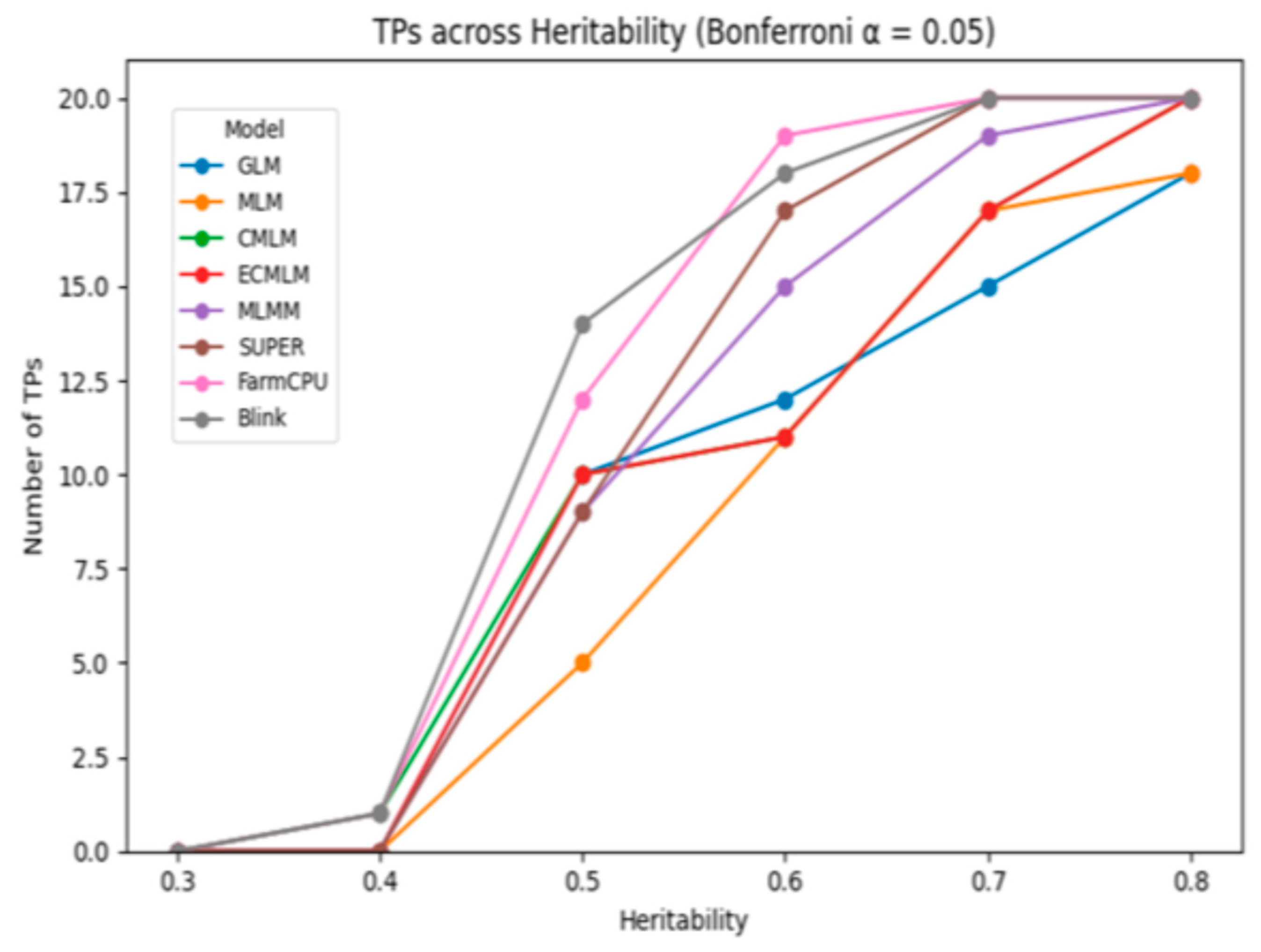
Figure 2. True positives (TPs) identified by eight GWAS models across increasing heritability levels (h² = 0.3–0.8) under Bonferroni correction at α = 0.01. Multi-locus models, particularly BLINK and FarmCPU, showed superior detection power at moderate to high heritability, while performance declined across all models at low heritability levels.

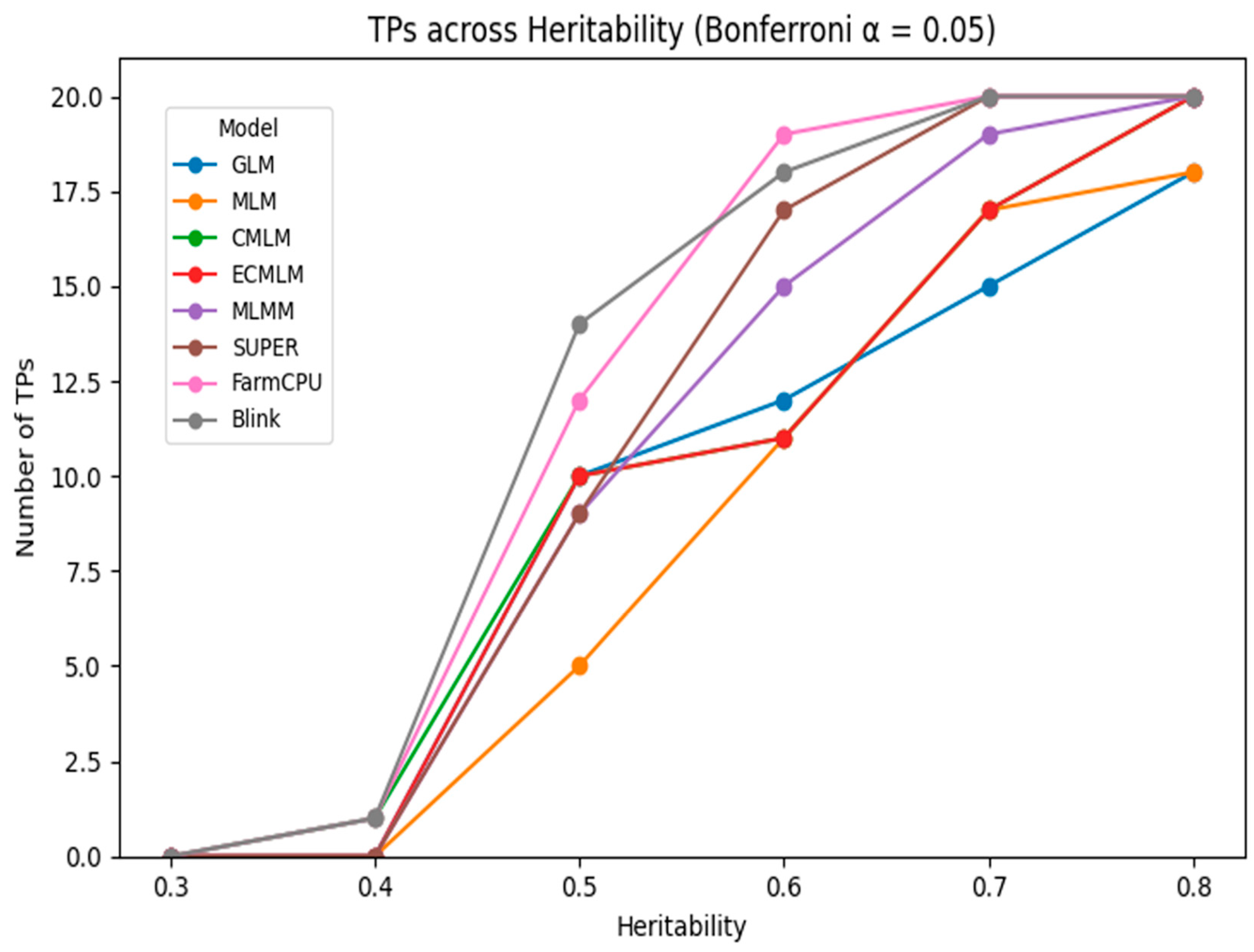
Figure 3. Quantile–quantile (Q–Q) plots of observed versus expected –log₁₀(p) values for eight GWAS models across Trait 1 and Trait 2. Departure from the diagonal indicates model-specific inflation or deflation of test statistics.

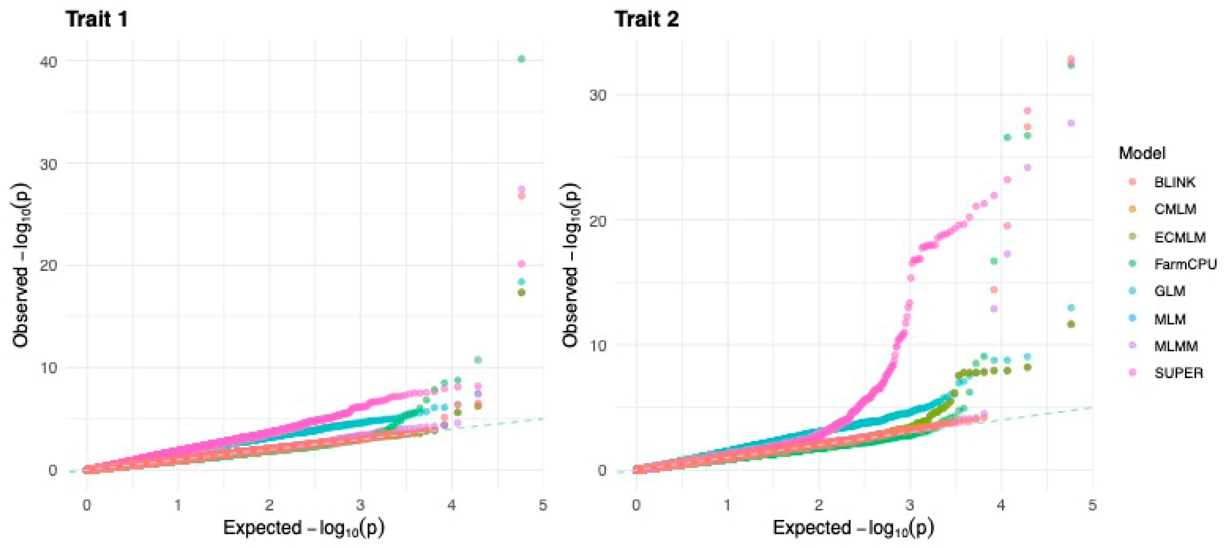
Figure 4. Power analysis of eight GWAS models for Trait 1 across varying Type I error thresholds. Most models exhibited increasing power with relaxed significance levels, with FarmCPU and CMLM achieving the highest detection power at the 10% error rate. The analysis highlights differences in sensitivity among methods, useful for selecting optimal models based on error tolerance in association mapping.

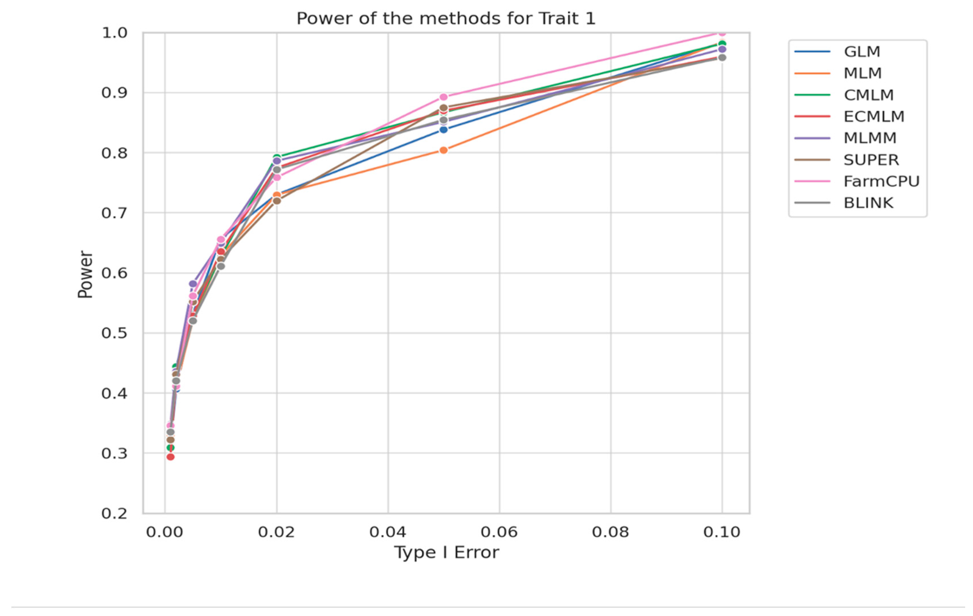
Figure 5. Comparison of average true positives (TPs) detected by BLINK, FarmCPU, and MLMM across two polygenicity levels (50 and 100 QTLs), averaged over 30 simulations. Error bars represent the standard deviation.

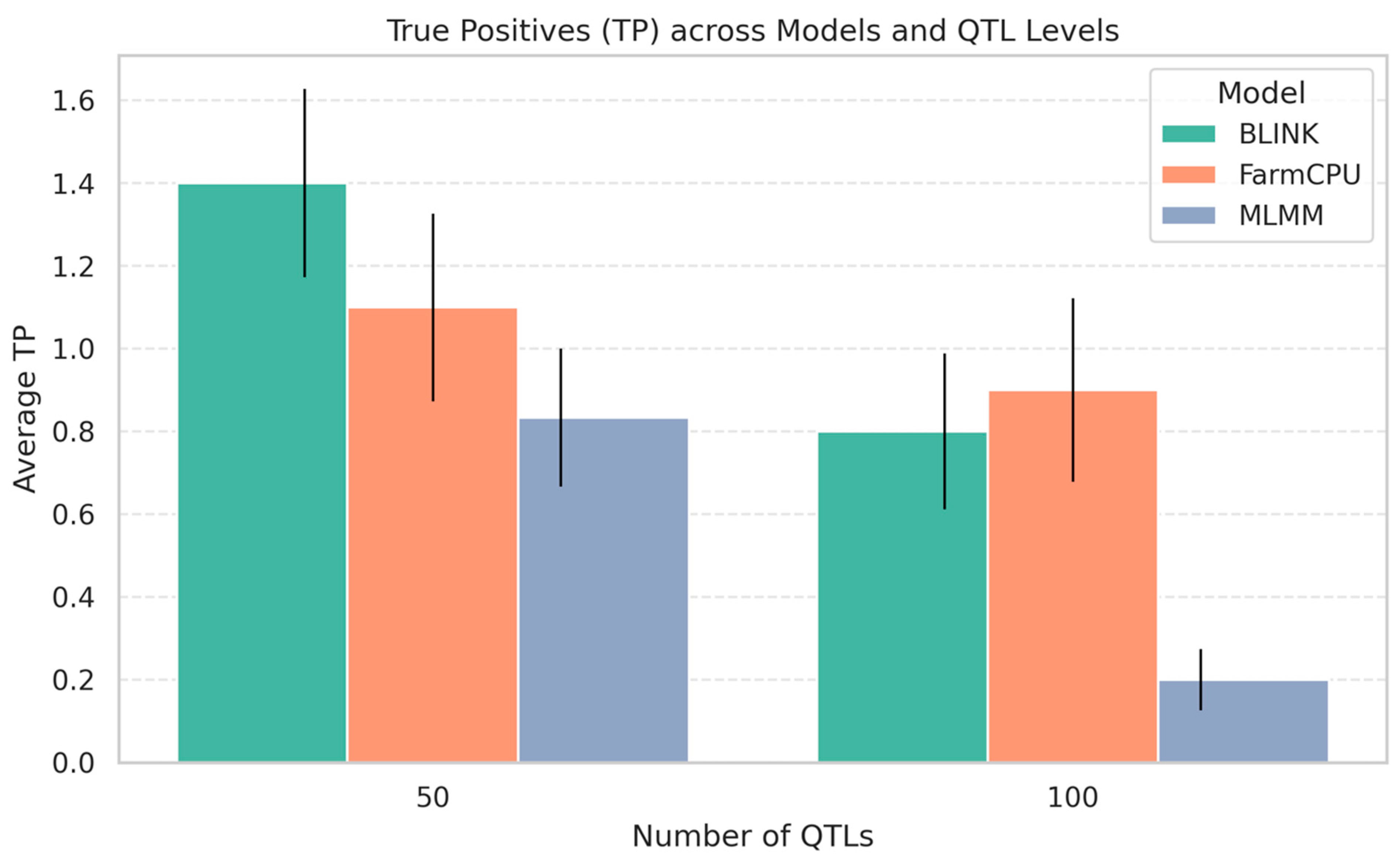
Figure 6. Comparison of mapping resolution (mean distance between significant SNPs and causal QTLs) for BLINK, FarmCPU, and MLMM at two polygenicity levels (50 and 100 QTLs), averaged across 30 replicates.

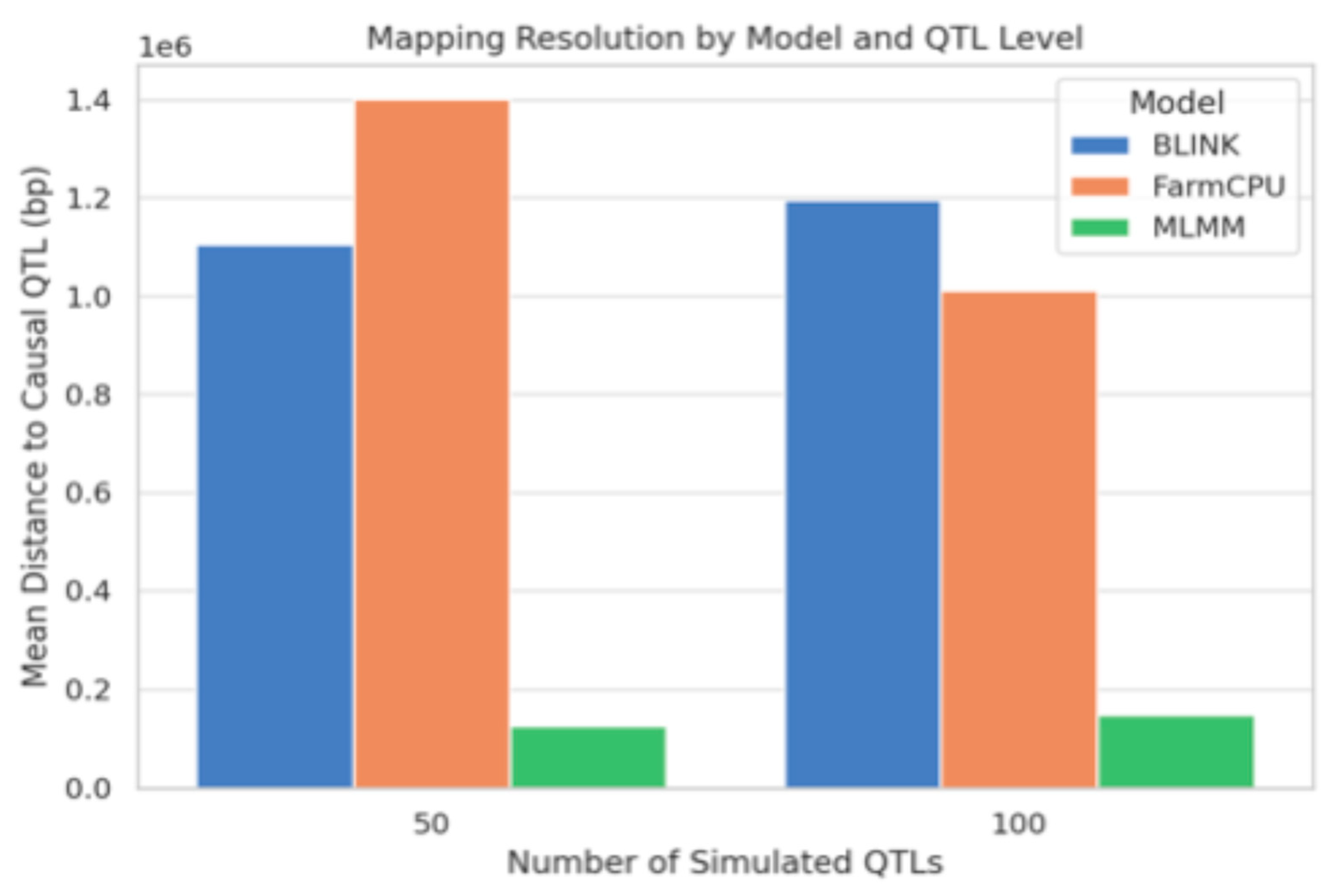
Table 1. General Features of GWAS models.

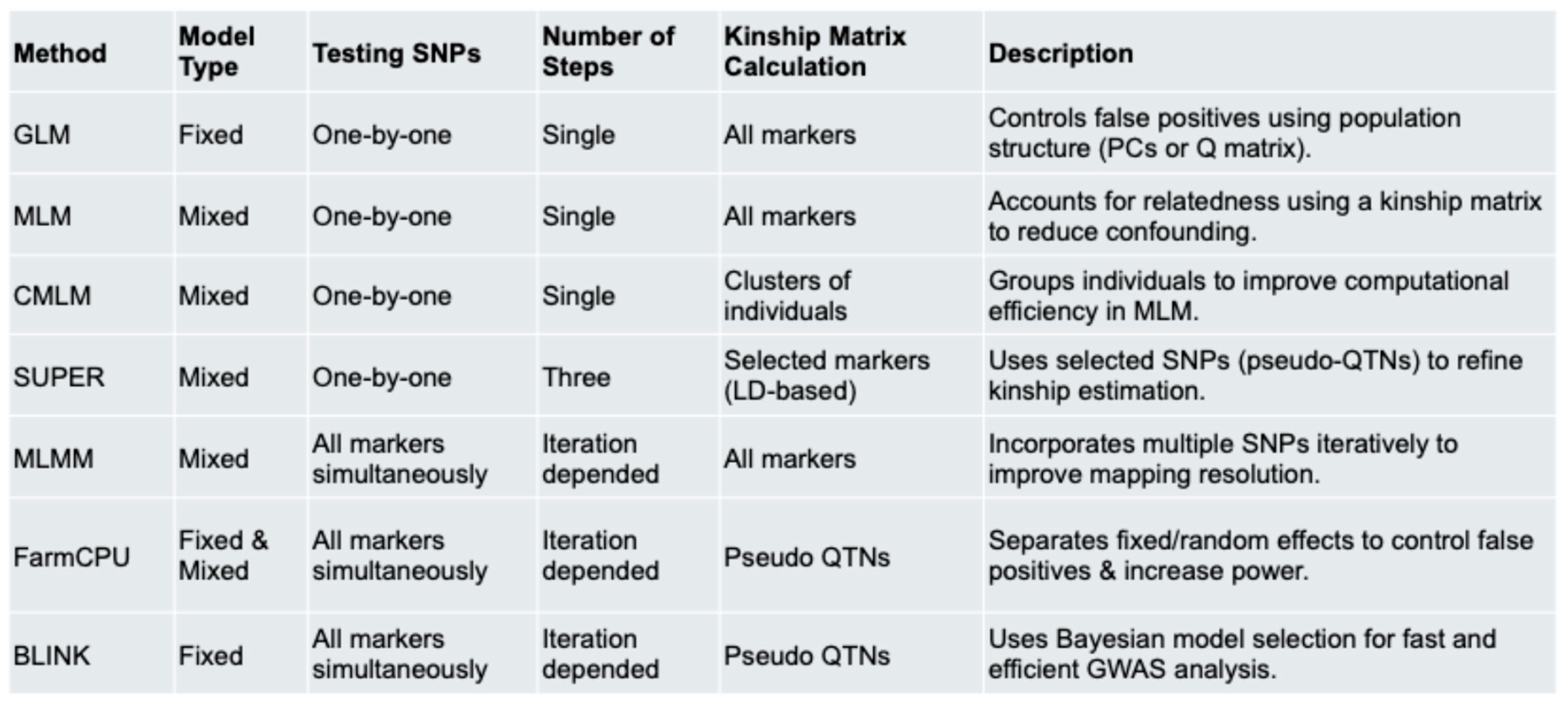Table 2. Genome Inflation values.

Model	Trait1_h2_0.3	Trait1_h2_0.5	Trait1_h2_0.8	Trait2_h2_0.3	Trait2_h2_0.5	Trait2_h2_0.8
GLM	1.292	3.496	2.098	1.429	2.979	1.933
MLM	0.986	1.001	0.986	0.99	1.023	0.972
CMLM	0.968	1.001	0.986	0.99	1.023	1.019
ECMLM	0.986	1.001	0.986	0.99	1.023	0.972
SUPER	1.01	1.439	2.85	1.225	1.046	1.475
MLMM	0.924	1.005	0.991	0.986	1.004	1.004
FarmCPU	0.938	0.821	0.87	0.883	0.944	0.796
BLINK	1.134	0.972	1.047	0.958	1.01	0.876

Disclaimer/Publisher’s Note: The statements, opinions and data contained in all publications are solely those of the individual author(s) and contributor(s) and not of MDPI and/or the editor(s). MDPI and/or the editor(s) disclaim responsibility for any injury to people or property resulting from any ideas, methods, instructions or products referred to in the content.

© 2025 by the authors. Licensee MDPI, Basel, Switzerland. This article is an open access article distributed under the terms and conditions of the Creative Commons Attribution (CC BY) license (http://creativecommons.org/licenses/by/4.0/).

Copyright: This open access article is published under a Creative Commons CC BY 4.0 license, which permit the free download, distribution, and reuse, provided that the author and preprint are cited in any reuse.