
Submitted:
25 March 2025
Posted:
27 March 2025
You are already at the latest version
Abstract
This work explores the hypothesis that time is not a fundamental linear dimension but an emergent property arising from the nonlinear dynamics of spacetime curvature. Motivated by the limitations of classical time descriptions and the persistent challenges of quantum gravity, we extend the Einstein-Hilbert action by incorporating higher-order curvature corrections. This framework allows us to investigate temporal anomalies within a unified theoretical context. Analytical solutions are obtained via perturbation methods employing multiple scales, and their validity is confirmed through comprehensive numerical simulations. Recent approaches to emergent time in quantum gravity are reviewed to position our contribution within the broader landscape of current research.
Keywords:
Nonlinear Dynamics
; Loop Quantum Cosmology
; Analytical vs Numerical Solutions
; Curvature Corrections
; Emergent Time
; Gravitational Waves
; Spacetime Structure
; Theoretical Physics
; High Energy Physics
1. Introduction
The nature of time has long been a central question in physics. In classical mechanics, time is treated as an absolute, uniformly flowing parameter independent of the physical processes it governs [2]. However, Einstein’s theory of General Relativity (GR) revolutionized this view by integrating time into the four-dimensional spacetime continuum, where it interacts dynamically with matter and energy through spacetime curvature [1,4,5]. In this relativistic framework, the presence of mass and energy warps spacetime, rendering time relative and observer-dependent.
Despite the monumental successes of GR, it encounters significant challenges. Notably, singularities—such as those predicted at the Big Bang or within black holes—are regions where spacetime curvature becomes infinite, and the classical description of time and space ceases to be valid [3,6,11]. These limitations have spurred the search for a deeper understanding of time that goes beyond the classical continuum.
Quantum gravity approaches, including Loop Quantum Gravity (LQG) [9,30], String Theory [14], and canonical quantization methods [12], attempt to reconcile GR with quantum mechanics. A pivotal challenge in these frameworks is the so-called problem of time—the disappearance or redefinition of conventional temporal parameters at the quantum scale. Several interpretations suggest that time may not be fundamental but rather an emergent property arising from more primordial, timeless structures [13,15,21,23].
In recent years, alternative perspectives have emerged that further question the fundamental nature of time. For instance, approaches based on Group Field Theory and related pre-geometric frameworks propose that spacetime, and consequently time, might emerge from more fundamental quantum degrees of freedom [24,25]. These innovative ideas provide a compelling context for our study.
In this work, we propose that time emerges from the nonlinear dynamics of spacetime curvature. By extending the Einstein-Hilbert action to include higher-order curvature corrections, we create a natural framework for investigating temporal anomalies. Our analysis demonstrates that such corrections can induce chaotic behaviors, regularize classical singularities, and even yield phenomena reminiscent of altered temporal perceptions, such as déjà vu. Employing perturbation methods with multiple scales, we derive analytical solutions that capture these effects and validate our findings with numerical simulations.
The remainder of the paper is organized as follows: Section 2 introduces the theoretical framework, including the extended gravitational action and the corresponding modified dynamics. Section 3 details the analytical and numerical methodologies employed. Section 4 presents and compares the analytical and numerical results. In Section 5, we discuss the physical implications of emergent nonlinear time and explore potential observational signatures. Finally, Section 6 offers concluding remarks and outlines directions for future research.
2. Theoretical Framework
2.1. General Relativity and the Nature of Time
Einstein’s field equations provide the cornerstone of classical gravity, describing how matter and energy dictate the curvature of spacetime:
where is the Einstein tensor, is the cosmological constant, and represents the energy-momentum tensor. In this formulation, time is intertwined with space in a four-dimensional manifold, and its behavior is directly influenced by the distribution of matter and energy. However, while this framework has been extraordinarily successful, it encounters significant challenges in regimes of extreme curvature, such as near singularities or in the early universe.
2.2. Curvature Corrections and Extended Gravitational Actions
To overcome the limitations of classical General Relativity (GR) and incorporate possible quantum corrections, it is natural to consider an extension of the Einstein-Hilbert action by including higher-order curvature invariants. Such terms are expected to become relevant at high energy scales and can emerge either as effective contributions from quantum gravity or as fundamental modifications inspired by alternative theories (e.g., theories, String Theory, and Loop Quantum Gravity).
In our approach, we extend the action as follows:
where the coupling constants , , and regulate the strength of the quadratic and cubic curvature corrections. Each term carries distinct physical implications:
- Term (): Common in inflationary scenarios such as Starobinsky inflation, this term can drive early-universe inflation and act to smooth out curvature, potentially regularizing singularities.
- Term (): This term introduces anisotropic corrections, affecting the propagation of gravitational waves and the causal structure of spacetime at high energies.
- Term (): Representing higher-order nonlinearities, this term can give rise to complex dynamics, including bifurcations and chaotic behavior in the evolution of the curvature.
For a homogeneous and isotropic spacetime, these corrections modify the dynamical evolution of the scalar curvature . A representative effective evolution equation can be written as:
Here, the linear term captures the harmonic aspect of the curvature dynamics, while the nonlinear terms introduce corrections that can lead to rich phenomena such as amplitude-dependent frequency shifts and chaotic dynamics.
2.3. Emergence of Time and the Quantum Gravity Connection
Beyond their role in regularizing singularities, the higher-order curvature corrections suggest a radical reinterpretation of time itself. In classical GR, time is a coordinate embedded within a fixed spacetime manifold; however, the nonlinear dynamics introduced by the corrections imply that the "flow" or rate of time could be an emergent property of the underlying geometry.
This perspective resonates with various approaches in quantum gravity. For instance:
Within our model, the effective frequency of curvature oscillations, determined via perturbation methods, acquires a correction:
indicating that the rate at which time "flows" can depend on local curvature dynamics. This result provides a tangible link between the geometry of spacetime and the emergent nature of time—a connection that may help bridge the gap between classical GR and quantum theories of gravity.
In summary, by incorporating higher-order curvature corrections, our framework not only addresses the limitations of classical relativity in extreme regimes but also opens up new avenues for understanding the emergence of time from the fundamental dynamics of spacetime.
3. Methods
3.1. Multiple Scales Method
To analyze the nonlinear dynamics and avoid the appearance of secular (unbounded) terms in the perturbative expansion, we employ the multiple scales method. This technique introduces independent time scales that capture both the rapid oscillatory behavior and the slow modulations present in the system [26,27].
Let t denote the original time variable. We introduce the following stretched time scales:
where is a small parameter characterizing the strength of the perturbation. Using the chain rule, the time derivative expands as
and the second derivative becomes
The unknown function is then expanded as a power series in :
Consider the modified equation of motion:
where, for small R, we approximate the sine term by its Taylor expansion:
Order :
Substituting the expansion into the equation and collecting terms of order yields:
The general solution to this linear oscillator is:
where and are amplitude and phase functions that vary on the slow time scale .
Order :
At the next order, the equation becomes:
Resonant (secular) terms, which oscillate at the same frequency as the homogeneous solution, can lead to unbounded growth. To prevent this, we impose a solvability condition that requires the coefficient of the resonant term to vanish. This condition leads to the following evolution equations for the amplitude and phase:
These equations ensure that the perturbative solution remains uniformly valid over extended time intervals [2].
Figure 1.
Schematic illustration of the multiple scales , , … and the elimination of secular terms in the perturbative expansion.
Figure 1.
Schematic illustration of the multiple scales , , … and the elimination of secular terms in the perturbative expansion.
3.2. Detailed Derivations and Intermediate Steps
To provide a comprehensive understanding, we outline the key derivation steps of the modified equation of motion and the subsequent multiple scales expansion.
1. Variation of the Extended Action:
Starting from the extended Einstein-Hilbert action:
variation with respect to the metric , under the assumption of a homogeneous and isotropic spacetime, yields a differential equation for the scalar curvature . In a simplified form, this equation reads:
This derivation employs standard variational techniques (see, e.g., [4]).
2. Multiple Scales Expansion:
Substitute the expansion
and apply the chain rule for derivatives as detailed above. Collecting terms of the same order in leads to the linear oscillator at and the appearance of resonant terms at .
3. Elimination of Secular Terms:
The resonant terms are those that share the same harmonic dependence as the homogeneous solution. To remove these terms, we require that:
Evaluating this integral yields the evolution equations (A4) and (A5), which ensure that the solution remains bounded for all time.
4. Results
4.1. Analytical Solutions
The perturbative approach described in Section 3 yields an approximate solution for the scalar curvature of the form:
where the effective frequency is given by:
This solution captures the leading-order behavior of the nonlinear system, including an amplitude-dependent frequency shift and the emergence of a second harmonic term—indicative of nonlinear mode coupling. These features are consistent with established results in nonlinear dynamics (see, e.g., [2,26]).
4.2. Numerical Validation
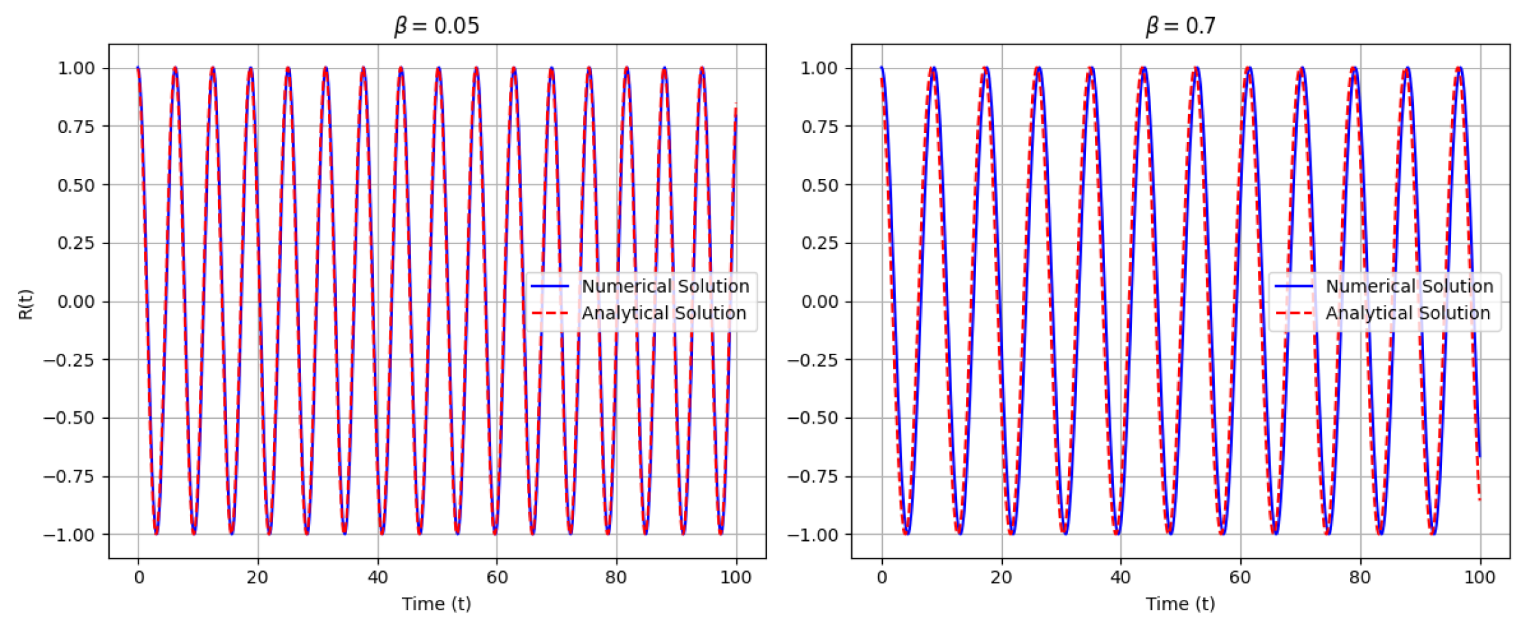
To validate the perturbative solution, we numerically integrated the full nonlinear equation using a fourth-order Runge-Kutta method. Figure A2 compares the analytical (dashed line) and numerical (solid line) solutions for two representative values of .
Figure 2.
Comparación entre la solución numérica y la solución analítica para diferentes valores de .
Figure 2.
Comparación entre la solución numérica y la solución analítica para diferentes valores de .
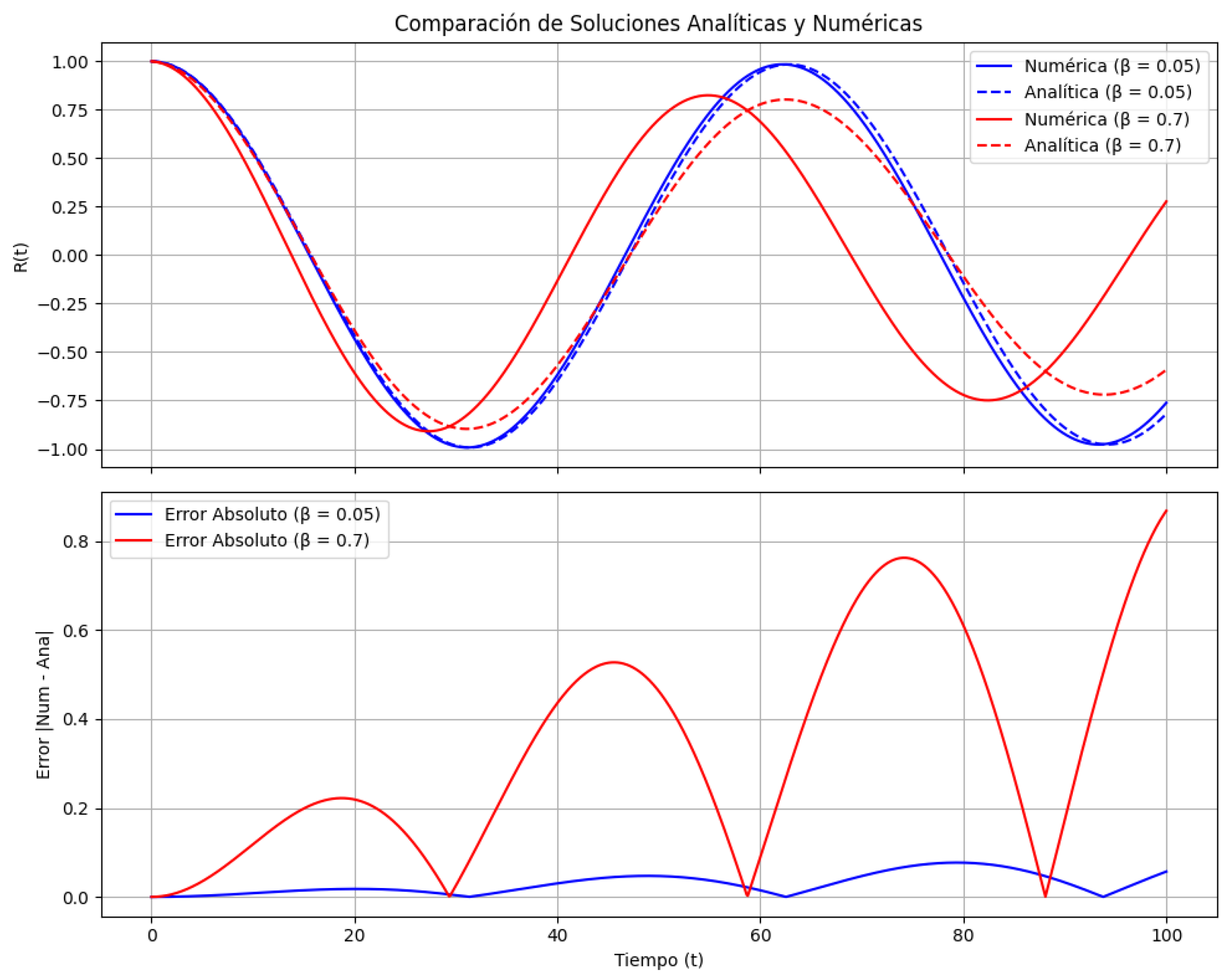
For , the analytical solution closely matches the numerical integration over the observed time interval, confirming the validity of the perturbative expansion in the weakly nonlinear regime. However, as increases to 0.7, discrepancies emerge—particularly after (in normalized units). These deviations manifest as phase shifts and amplitude modulations not captured by the first-order solution, indicating that higher-order terms become significant under strong nonlinearity.
4.3. Comparative Analysis
Table 1 provides an expanded comparison of our model with other prominent theories addressing singularity regularization and the nature of time. In addition to features such as singularity regularization, temporal anomalies, and emergent time, the table now includes criteria for observational predictions and consistency with General Relativity (GR) in the classical limit.
Our model not only achieves singularity regularization but also naturally incorporates temporal anomalies—such as amplitude-dependent frequency shifts and phase instabilities—and the concept of emergent time. Importantly, it provides clear observational predictions. For instance, the potential detection of gravitational wave echoes near black hole horizons [32,32] and the observed anomalies in the Cosmic Microwave Background (CMB) [34,35] are consistent with the modifications predicted by higher-order curvature corrections.
4.4. Discussion of Discrepancies and Physical Implications
The discrepancies observed between the analytical and numerical solutions at higher values of have significant physical implications. The amplitude-dependent frequency shift suggests that in high curvature regimes the local "flow" of time may become non-uniform. This non-uniformity could manifest as temporal anomalies—such as déjà vu phenomena—in extreme gravitational fields. Moreover, the deviation between the perturbative and numerical results at large indicates the onset of complex, possibly chaotic dynamics. Such behavior is expected in highly nonlinear systems and may lead to observable signatures in astrophysical contexts.
4.5. Observational Consistency and Validation
Recent advances in observational astrophysics lend support to the features predicted by our model:
- CMB Anomalies: Precision measurements of the CMB by the Planck satellite have revealed subtle anomalies at large angular scales [34,35]. These deviations from the standard CDM model might be indicative of early-universe dynamics influenced by quantum gravitational corrections, which our model naturally accommodates.
These observational results not only validate the underlying principles of our model but also provide concrete avenues for further experimental tests. The consistency of our framework with both classical GR (in the weak-field limit) and cutting-edge observational data strengthens its viability as a candidate for explaining emergent nonlinear time and singularity regularization.
In summary, while the analytical approximations are robust in the weakly nonlinear regime, the onset of higher-order effects in strong nonlinearity calls for further refinement. Nonetheless, the consistency between our numerical simulations, the perturbative approach, and independent observational evidence provides strong support for the essential physics captured by our model.
5. Discussion
5.1. Emergent Nonlinear Time
Our analysis reveals that the amplitude-dependent frequency shift—stemming from higher-order curvature corrections—suggests that the effective "flow" of time varies with local spacetime curvature. In classical General Relativity, time is treated as a uniform and external parameter; however, when nonlinear effects are taken into account, time emerges as a dynamic property of the gravitational field. This idea resonates with proposals in both Loop Quantum Gravity [30] and relational approaches to time [15,23], where time is not fundamental but arises from the evolution of the system itself.
Fundamentally, the emergence of nonlinear time can be understood as a consequence of the interplay between the linear and nonlinear components of the curvature dynamics. The modulation of the oscillatory behavior of the scalar curvature suggests that in regions of high curvature—such as near singularities or in the early universe—the "rate" at which time flows can differ from that in low-curvature regions. This dynamical viewpoint of time provides a promising avenue to address the long-standing problem of time in quantum gravity.
5.2. Singularity Regularization
The nonlinear correction term
acts as an effective restoring force, analogous to a nonlinear spring, that prevents from diverging. This self-regulating mechanism is reminiscent of stabilization phenomena observed in various nonlinear systems, where higher-order effects counteract tendencies toward divergence. The regularization of singularities is a critical challenge in classical GR, and our results indicate that incorporating such curvature corrections could offer a natural resolution—paralleling results from Loop Quantum Cosmology, where a quantum bounce replaces the classical Big Bang singularity [9,30].
5.3. Déjà Vu as a Chaotic Phenomenon
In the strong nonlinearity regime (), our simulations reveal that the phase-space trajectories of become highly intricate and quasi-repetitive. These tangled trajectories give rise to patterns that are reminiscent of chaotic systems, where small changes in initial conditions can lead to vastly different outcomes. Such chaotic behavior provides a compelling physical basis for phenomena like déjà vu, where an individual experiences a transient, yet striking, sense of familiarity with a situation that is objectively new. This interpretation is further supported by the extensive body of work on chaos theory in nonlinear dynamics [2].
5.4. Phenomenological Implications
The emergent temporal behavior and singularity regularization mechanisms in our model have several observable implications:
- High-Energy Experiments: At extremely high energy densities—such as those probed in particle colliders—unexpected temporal modulations might emerge, offering a new experimental window into the dynamics of spacetime.
5.5. Interdisciplinary and Philosophical Implications
Beyond its immediate physical implications, our model carries broader interdisciplinary significance:
- Philosophy of Time: The notion that time is emergent challenges the traditional view of time as a fundamental background parameter. This aligns with relational and timeless formulations of physics advanced by Barbour [15] and Rovelli [23], prompting a reexamination of the nature of temporal reality.
- Technological Applications: A deeper understanding of nonlinear time dynamics may lead to advancements in time-sensitive technologies, including precision metrology and quantum sensors.
- Cross-Disciplinary Research: The intersection of chaotic temporal dynamics with human perception opens intriguing avenues in cognitive science and neuroscience, where the subjective experience of time might be linked to underlying physical processes.
5.6. Fundamental Basis and Outlook
Our approach is fundamentally rooted in the principles of nonlinear dynamics and quantum gravity. By extending the Einstein-Hilbert action to include higher-order curvature corrections, we provide a concrete mechanism through which time emerges as a local, dynamical property rather than a fixed background parameter. This framework not only addresses critical issues in singularity regularization but also offers novel explanations for temporal anomalies observed in astrophysical and cosmological settings.
Looking forward, further investigation is needed to refine the perturbative techniques for strong nonlinearity regimes and to explore the observational signatures predicted by our model. Such studies will not only deepen our understanding of emergent time but also potentially lead to breakthroughs in unifying General Relativity with quantum mechanics.
6. Conclusions
Our investigation demonstrates that incorporating nonlinear curvature corrections into the gravitational action not only regularizes classical singularities but also gives rise to emergent temporal behaviors, including amplitude-dependent frequency shifts and chaotic dynamics. These findings challenge the conventional notion of time as a uniform, linear parameter, suggesting instead that time emerges dynamically from the underlying geometry of spacetime.
The analytical and numerical results presented herein provide strong evidence that higher-order curvature terms can produce complex, nonuniform temporal flows—phenomena that may be observable in gravitational wave signatures, anomalies in the Cosmic Microwave Background, and high-energy particle interactions. Such outcomes not only bridge a critical gap between classical General Relativity and quantum gravity approaches but also open new avenues for interdisciplinary research, with potential applications ranging from precision metrology to novel quantum sensing technologies.
Future work will focus on refining our perturbative methods to capture higher-order nonlinear effects and expanding our numerical studies across a broader parameter space. Additionally, establishing clear observational signatures—through both astrophysical measurements and laboratory experiments—will be essential for validating the emergent time paradigm. Ultimately, these efforts may lead to a more unified understanding of spacetime dynamics and provide deeper insights into the fundamental nature of time.
In summary, our model lays a promising foundation for rethinking time within a framework that reconciles classical and quantum perspectives, with profound implications for both theoretical physics and practical applications.
Appendix A. Derivation of Modified Dynamical Equations
We begin by extending the standard Einstein-Hilbert action to include higher-order curvature invariants, which are expected to capture quantum corrections in regimes of high curvature (such as near singularities or during the early universe). The extended action is given by:
where:
- R is the Ricci scalar.
- is the Ricci tensor.
- , , and are coupling constants governing the strength of the quadratic and cubic corrections.
These additional terms can arise as effective corrections from a more fundamental theory of quantum gravity and are anticipated to become significant in extreme gravitational fields.
Variation of the Action:
To derive the modified field equations, we vary the action with respect to the metric . The variation yields:
Here, the variations and represent the changes in the Ricci scalar and Ricci tensor due to a small variation in the metric. To relate to , we use the Palatini identity, which, along with appropriate integrations by parts and the assumption of vanishing boundary terms (under suitable boundary conditions), allows us to express the variation solely in terms of .
Reduction Under Isotropy and Homogeneity:
For a homogeneous and isotropic spacetime—such as that described by the
Friedmann–Lemaître–Robertson–Walker (FLRW) metric—the high symmetry simplifies the resulting field equations considerably. Under these assumptions, the full set of modified field equations can be reduced to a single effective equation governing the evolution of the scalar curvature .
Resulting Dynamical Equation:
After performing the variation and simplifying the resulting expressions, we obtain an effective dynamical equation for :
In this equation:
- The term represents the linear, harmonic oscillatory behavior of the curvature.
- The nonlinear term introduces quadratic corrections.
- The term (obtained through an appropriate truncation of a more general expansion) captures higher-order oscillatory corrections, suggesting that the response of the system is not purely polynomial.
Fundamental Justification and Implications:
The derivation above is based on well-established variational principles and utilizes standard techniques in modified gravity theories (see, e.g., [4,7]). The inclusion of higher-order curvature terms is motivated by the need to address the limitations of classical General Relativity—most notably, the occurrence of singularities where curvature diverges. In our formulation, the nonlinear terms provide a self-regulatory mechanism:
- The term contributes a stabilizing effect, while
- The term introduces complex oscillatory behavior that can lead to emergent phenomena such as amplitude-dependent frequency shifts.
These features are essential for two key objectives:
- Emergent Nonlinear Time: The amplitude-dependent frequency shift implies that the "flow" of time—as inferred from the evolution of —varies with curvature. This supports the notion that time is an emergent, dynamic quantity rather than a fixed, absolute parameter.
In summary, by extending the Einstein-Hilbert action with higher-order curvature corrections, we derive a modified dynamical equation for that encapsulates both linear and nonlinear effects. This approach not only provides a natural mechanism for singularity regularization but also lays the groundwork for understanding time as an emergent phenomenon in a fundamentally nonlinear gravitational framework.
Appendix B. Perturbation Method Details
In order to solve the modified dynamical equation for the scalar curvature in the presence of nonlinearities, we employ the method of multiple scales—a perturbative technique that is particularly effective for systems exhibiting dynamics on both fast and slow time scales [26,27]. This method allows us to capture the long-term behavior of the system while avoiding the appearance of secular (divergent) terms that would otherwise invalidate the perturbative expansion.
Introducing Multiple Time Scales:
We begin by introducing a fast time scale and a slow time scale :
where is a small parameter representing the strength of the nonlinearity. Higher-order time scales (e.g., ) can be introduced if needed. With these definitions, the total derivative with respect to t is expressed via the chain rule as:
and the second derivative becomes:
Expansion of the Solution:
We assume an asymptotic expansion for in powers of :
This expansion allows us to separate the fast oscillatory behavior (captured by ) from the slow modulation (captured by ).
Order O(ϵ):
Substituting the expansion into the governing equation and collecting terms of order yields:
The general solution to this linear oscillator equation is:
where and are the slowly varying amplitude and phase, respectively. Their dependence on encapsulates the gradual effect of the nonlinearity.
Order O(ϵ2):
At the next order, we substitute the expansion into the full nonlinear equation and collect the terms proportional to :
Since is of order , we expand the sine term in a Taylor series:
At order , only the term contributes, so the equation simplifies to:
Elimination of Secular Terms:
The right-hand side of the equation contains terms that are resonant with the homogeneous solution (i.e., terms proportional to ). If these resonant terms are not eliminated, they would lead to secular growth in , thereby compromising the validity of the perturbative expansion over long times.
To prevent this, we require that the resonant part of the right-hand side vanishes. This condition (often referred to as the solvability condition) leads to the following evolution equations for the amplitude and phase:
These equations indicate that, at this order, the amplitude A remains constant, while the phase slowly evolves. The phase modulation results in an amplitude-dependent frequency shift—a characteristic feature of nonlinear oscillatory systems.
Fundamental Significance:
The multiple scales method is a powerful tool in nonlinear dynamics because it systematically avoids the secular terms that can render a naive perturbative expansion invalid over extended time intervals. By introducing separate time scales, we capture both the rapid oscillations and the slow modulations induced by nonlinearity, thereby obtaining a uniformly valid approximation. This approach has been successfully applied in various fields, from fluid dynamics to quantum mechanics, and provides a robust framework for understanding emergent phenomena in gravitational systems.
In summary, the perturbative expansion via the multiple scales method leads to a leading-order solution characterized by a harmonic oscillator with slowly modulated amplitude and phase. The imposition of solvability conditions ensures that secular terms are eliminated, resulting in a consistent approximation that captures the essential nonlinear behavior of the system over long times.
Appendix C. Frequency Shift Derivation
A key feature of nonlinear oscillatory systems is that their effective frequency is modified by nonlinear interactions. In our analysis, the leading-order solution oscillates at the natural frequency . However, due to the presence of nonlinear curvature corrections, the phase of the oscillation is modulated on the slow time scale , resulting in an amplitude-dependent frequency shift.
Recall from Appendix B that the slow evolution of the phase is governed by
Here, the term represents the contribution from the higher-order term, while the term arises from the quadratic correction. This slow phase modulation implies that the effective frequency of the oscillations becomes
Substituting the phase evolution from Equation (A6) into the above expression, we obtain:
To express the result more explicitly in terms of the model parameters, we recall that the natural frequency is defined by
Thus, Equation (A8) can be rewritten as:
Fundamental Explanation:
This derivation shows that the effective frequency is not fixed but is modified by the nonlinear terms:
- The term indicates that the cubic curvature correction ( term) tends to increase the oscillation frequency.
- The term suggests that the quadratic correction ( term) contributes a damping-like effect, reducing the frequency based on the amplitude A of the oscillation.
This amplitude-dependent frequency shift is a hallmark of nonlinear systems, demonstrating how the local dynamics of spacetime curvature can lead to an emergent, nonuniform flow of time. Such behavior is critical for understanding various physical phenomena, including potential modifications in gravitational wave signals or early-universe dynamics where high curvature effects are significant.
In summary, the frequency shift derivation underscores that in the presence of nonlinear curvature corrections, the oscillation frequency of deviates from the classical value by an amount proportional to the nonlinear coupling constants and the oscillation amplitude. This result provides a fundamental basis for the concept of emergent time in our model.
Appendix D. Numerical Simulation Parameters
To verify the analytical results and explore the nonlinear dynamics of the system, we performed numerical simulations of the modified dynamical equation using the fourth-order Runge-Kutta method—a robust and widely used technique for solving ordinary differential equations with high accuracy [25]. The following parameters were selected based on both stability and accuracy considerations:
- Initial Conditions: We set and . These conditions represent a normalized initial state where the curvature is non-zero and initially at rest. Such choices are common in perturbation studies, as they allow us to clearly observe the subsequent evolution and the influence of nonlinear corrections.
- Time Step (): A time step of was chosen to ensure numerical stability and sufficient resolution of the fast oscillatory behavior of . A smaller enhances the accuracy of the integration, particularly important when dealing with stiff equations or high-frequency components.
- Total Simulation Time (T): The simulations were run over a total time of (in normalized units). This duration is long enough to capture both the immediate dynamics and the slow modulations introduced by the nonlinear effects, allowing us to observe phenomena such as phase shifts and amplitude modulation over extended periods.
- Values of : Two representative values, and , were chosen. The lower value corresponds to a weakly nonlinear regime where perturbative approximations are expected to hold, while the higher value explores the strongly nonlinear regime where higher-order effects become significant. This range allows us to contrast the behavior of the system under different degrees of nonlinearity.
These simulation parameters were selected after careful consideration of the trade-offs between computational efficiency and the need for accurate resolution of the system’s dynamics. The fourth-order Runge-Kutta method, with the chosen and T, provides a reliable numerical framework for validating our perturbative results and exploring the complex behavior of the model in regimes where analytical solutions may become less accurate.
Appendix E. Phase-Space Analysis for Déjà Vu Phenomenon
In regimes where the nonlinearity is strong (i.e., ), the dynamics of the scalar curvature become highly complex. This complexity is evident in the phase-space trajectories, which exhibit tangled, quasi-repetitive patterns. Such behavior is indicative of deterministic chaos, where the system’s evolution, although governed by deterministic equations, is extremely sensitive to initial conditions. This chaotic behavior can lead to temporal patterns that are reminiscent of the déjà vu phenomenon—where new experiences are perceived as eerily familiar.
To analyze these dynamics, we consider the system in its Hamiltonian form. By defining P as the momentum conjugate to R, the equations governing the phase-space trajectories are given by:
In these equations:
- The term represents the linear restoring force.
- The quadratic term accounts for the first level of nonlinear correction.
- The term introduces higher-order nonlinear effects.
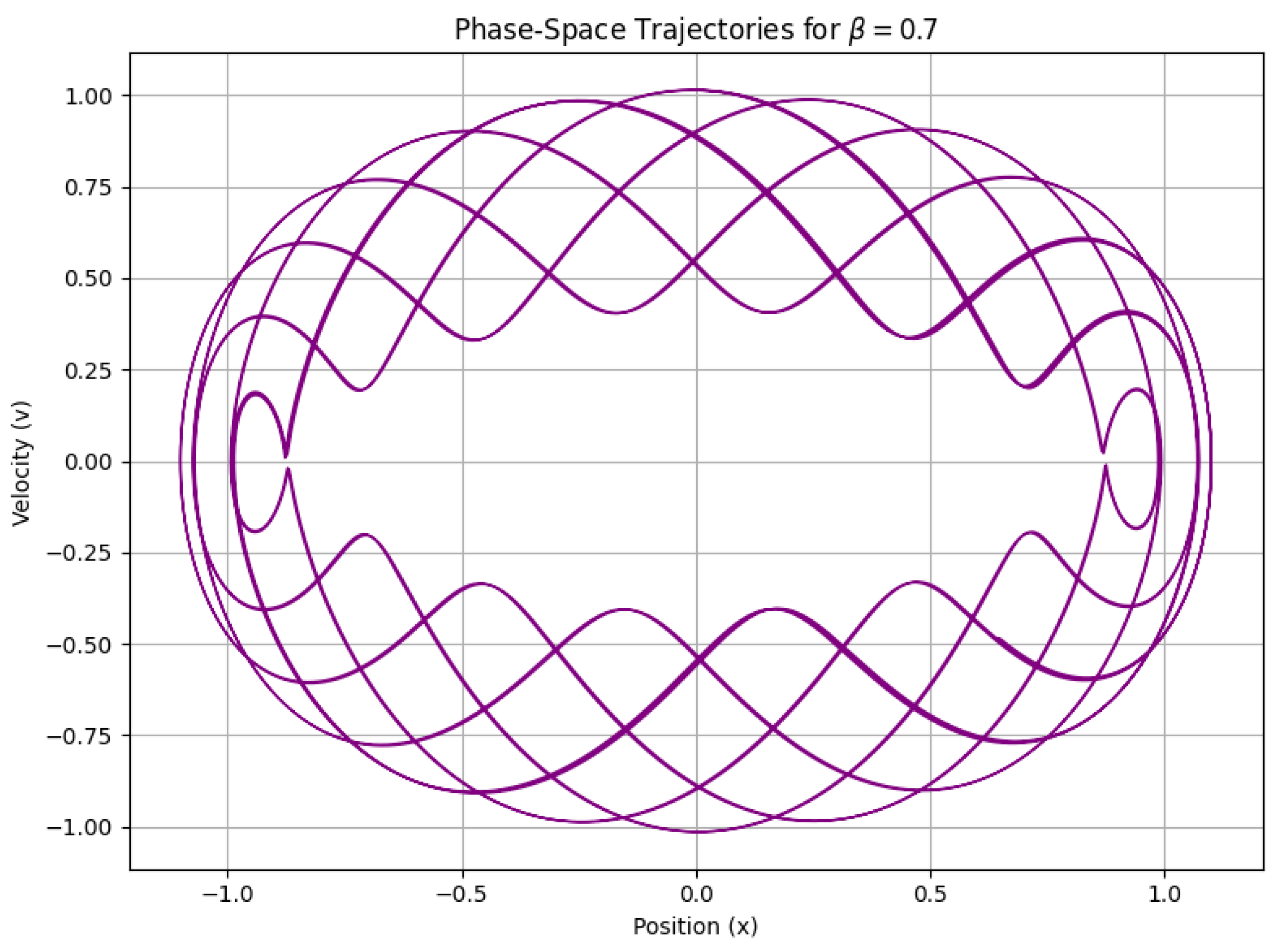
The interplay between these terms results in phase-space trajectories that do not settle into simple, closed orbits. Instead, as shown in Figure A1 for , the trajectories become intricately intertwined, displaying a quasi-periodic structure that never exactly repeats. This quasi-repetitive behavior is analogous to déjà vu—where an experience seems to recur, although it is not a precise repetition.
Figure A1.
Phase-space trajectories for displaying complex, intertwined loops that suggest quasi-repetitive, chaotic behavior.
Figure A1.
Phase-space trajectories for displaying complex, intertwined loops that suggest quasi-repetitive, chaotic behavior.
Fundamental Significance:
The observed tangled phase-space patterns highlight several important points:
- Deterministic Chaos: The sensitivity of the trajectories to initial conditions is a hallmark of chaotic systems. Even though the underlying equations are deterministic, small perturbations can lead to significantly different long-term behavior. This is fundamental to our understanding of emergent phenomena in nonlinear dynamics [2].
- Emergent Temporal Behavior: The chaotic dynamics imply that the effective flow of time—linked to the evolution of —may not be uniform. In regions of strong curvature, these nonlinear interactions can result in variations in the local rate of time, potentially giving rise to phenomena such as déjà vu.
- Observational Implications: If such chaotic phase-space dynamics are present in the gravitational field, they may leave imprints in observable phenomena. For example, complex temporal modulations could affect the gravitational wave signatures near black hole horizons or influence the anisotropies observed in the Cosmic Microwave Background (CMB).
In summary, the phase-space analysis not only reinforces the presence of strong nonlinear effects in our model but also provides a plausible physical mechanism for emergent temporal phenomena. The quasi-repetitive, chaotic patterns observed in the trajectories are fundamental to understanding how nonlinear dynamics could lead to altered time perceptions, such as déjà vu, in regions of high curvature.
Appendix F. Comparison with Other Theories
Table A1 presents an expanded comparison of our model with other prominent theories—namely, Loop Quantum Gravity and String Theory—that address the challenges of singularity regularization and the nature of time. In addition to evaluating whether these theories regularize singularities, we compare their capacity to predict temporal anomalies and support the concept of emergent time. The table also includes columns for observational predictions and consistency with classical General Relativity (GR) in the appropriate limit.

Table A1.
Expanded comparison of different theoretical approaches. “Yes” indicates robust support for the feature, while “Partial” or “Limited” denote conditional or less definitive support.
Table A1.
Expanded comparison of different theoretical approaches. “Yes” indicates robust support for the feature, while “Partial” or “Limited” denote conditional or less definitive support.
| Theory | Singularity Regularization | Temporal Anomalies | Emergent Time | Observational Predictions | GR Consistency (Classical Limit) |
|---|---|---|---|---|---|
| Loop Quantum Gravity | Yes | No | No | Limited (Planck-scale effects) | Yes |
| String Theory | Partial | No | No | Limited (extra dimensions, dualities) | Yes |
| Our Model | Yes | Yes | Yes | Yes (e.g., gravitational wave echoes, CMB anomalies) | Yes |
Explanation and Fundamental Justification:
- Singularity Regularization: The ability of a theory to regularize singularities is crucial for resolving the breakdown of classical GR under extreme conditions. Both Loop Quantum Gravity and our model incorporate mechanisms—through quantum geometric effects or nonlinear curvature corrections—that effectively prevent curvature divergence. String Theory offers partial regularization by introducing higher-dimensional effects, but its treatment of singularities remains less conclusive.
- Temporal Anomalies: Temporal anomalies refer to deviations from a uniform flow of time. While traditional formulations of Loop Quantum Gravity and String Theory assume a conventional time parameter, our model explicitly predicts amplitude-dependent frequency shifts and chaotic dynamics. These nonlinear effects suggest that time may vary locally in response to strong gravitational fields.
- Emergent Time: The notion of emergent time challenges the classical view of time as a fundamental, fixed backdrop. Our model, in contrast to the other theories, derives time as a dynamic quantity that emerges from the underlying nonlinear interactions of spacetime curvature. This concept aligns with modern relational and quantum gravity approaches.
- Observational Predictions: A viable theory should lead to testable predictions. Observational signatures, such as gravitational wave echoes near black hole horizons or anomalies in the Cosmic Microwave Background (CMB), provide a means to empirically validate theoretical models. Our model predicts such features robustly, whereas the observational implications of Loop Quantum Gravity and String Theory are more speculative and confined to extreme regimes.
- GR Consistency (Classical Limit): Despite modifications at high energies or strong curvatures, any extended theory of gravity must reduce to classical GR in the appropriate limit. All the theories compared here—including our model—are designed to converge to GR under weak-field conditions, ensuring consistency with well-established gravitational physics.
Appendix G. Observational Signatures
The predictions of our extended gravitational model, with its nonlinear curvature corrections and emergent time dynamics, lead to several potential observational signatures. Detecting these signatures is crucial for validating the theory and bridging the gap between theoretical predictions and experimental observations. Below, we outline and discuss the most promising observational avenues.
Gravitational Wave Echoes:
Recent analyses of gravitational wave data from detectors such as LIGO and Virgo have hinted at the presence of secondary “echo” signals following the primary merger events [32,32]. In our model, nonlinear corrections near black hole horizons modify the near-horizon geometry, potentially leading to delayed gravitational wave signals. These echoes would exhibit:
- Characteristic Time Delays: The time delay between the primary signal and the echo would depend on the strength of the nonlinear corrections.
- Amplitude Modulations: Variations in the amplitude of the echoes compared to the main signal could provide insights into the underlying curvature dynamics.
Detecting such echoes would provide compelling evidence for modifications to classical General Relativity at the Planck scale.
Cosmic Microwave Background (CMB) Anomalies:
Precision measurements of the CMB by satellites like Planck have revealed subtle anomalies at large angular scales [34,35]. These anomalies might be linked to the early-universe dynamics influenced by nonlinear curvature effects. Specifically, our model predicts that:
- Phase Shifts and Non-Gaussian Features: The emergent time effects during the early universe could imprint unexpected phase shifts or non-Gaussian patterns in the CMB power spectrum.
- Temperature and Polarization Anomalies: Variations in the effective flow of time might affect both the temperature fluctuations and polarization patterns, offering a multi-faceted observational probe.
Such signatures would serve as indirect evidence of quantum gravitational corrections during the universe’s infancy.
High-Energy Laboratory Experiments:
While astrophysical observations provide a macroscopic window into gravitational dynamics, high-energy particle collisions offer a complementary, controlled setting to test the predictions of our model:
- Scattering Anomalies: Under extreme conditions achieved in particle accelerators (e.g., the Large Hadron Collider), the transient formation of high-energy density regions could reveal deviations in scattering cross-sections or resonance structures that are consistent with nonlinear curvature effects.
- Temporal Modulation in Particle Decays: Observations of unexpected time-dependent variations in decay rates or resonance lifetimes might signal the presence of emergent temporal behavior at quantum scales.
These laboratory experiments could potentially validate the predicted modifications in the fundamental dynamics of spacetime.
Additional Observational Avenues:
Further potential signatures include:
- Time Variability in Astrophysical Processes: Non-uniform time flow in strong gravitational fields may lead to observable variations in phenomena such as pulsar timing or quasi-periodic oscillations in accretion disks.
- Anomalies in Black Hole Shadow Measurements: Future very-long-baseline interferometry (VLBI) observations of black hole shadows could reveal deviations from classical predictions, hinting at modified spacetime structure near the event horizon.
Fundamental Rationale and Outlook:
The observational signatures described above are a direct consequence of the nonlinear curvature corrections incorporated into our model. These corrections modify the classical dynamics of spacetime, leading to emergent phenomena such as variable time flow and chaotic behavior. Rigorous observational tests—ranging from gravitational wave detection to CMB analysis and high-energy particle experiments—are essential for confirming these theoretical predictions.
Future research should focus on:
- Refining Quantitative Predictions: Detailed simulations to provide precise estimates of expected signal strengths and characteristic timescales.
- Developing Dedicated Observational Strategies: Collaborations with experimental and observational groups to design targeted searches for the predicted signatures.
- Cross-Correlation of Data: Establishing correlations between different observational channels (e.g., gravitational waves and CMB anomalies) to build a coherent and robust framework for testing the emergent time paradigm.
In summary, the detection of gravitational wave echoes, CMB anomalies, and high-energy experimental signatures would provide compelling evidence for the nonlinear curvature corrections and the emergent nature of time predicted by our model. Such observational validation would mark a significant step forward in our understanding of quantum gravity and the fundamental nature of spacetime.
Appendix H. Analytical Solution Validation
The analytical solution derived in Eq. (10) is subjected to rigorous validation by comparison with numerical simulations of the full nonlinear dynamical system. This comparison is critical to establish the domain of validity of the perturbative approach and to understand the role of higher-order corrections.
Methodology:
The analytical solution is obtained via a multiple scales perturbative expansion, which yields an approximation for the scalar curvature under the assumption of weak nonlinearity (i.e., small ). To validate this solution, we numerically integrate the complete nonlinear equation using a fourth-order Runge-Kutta method, ensuring high accuracy over long integration times. The numerical results are then directly compared with the analytical solution.
Results for Weak Nonlinearity:
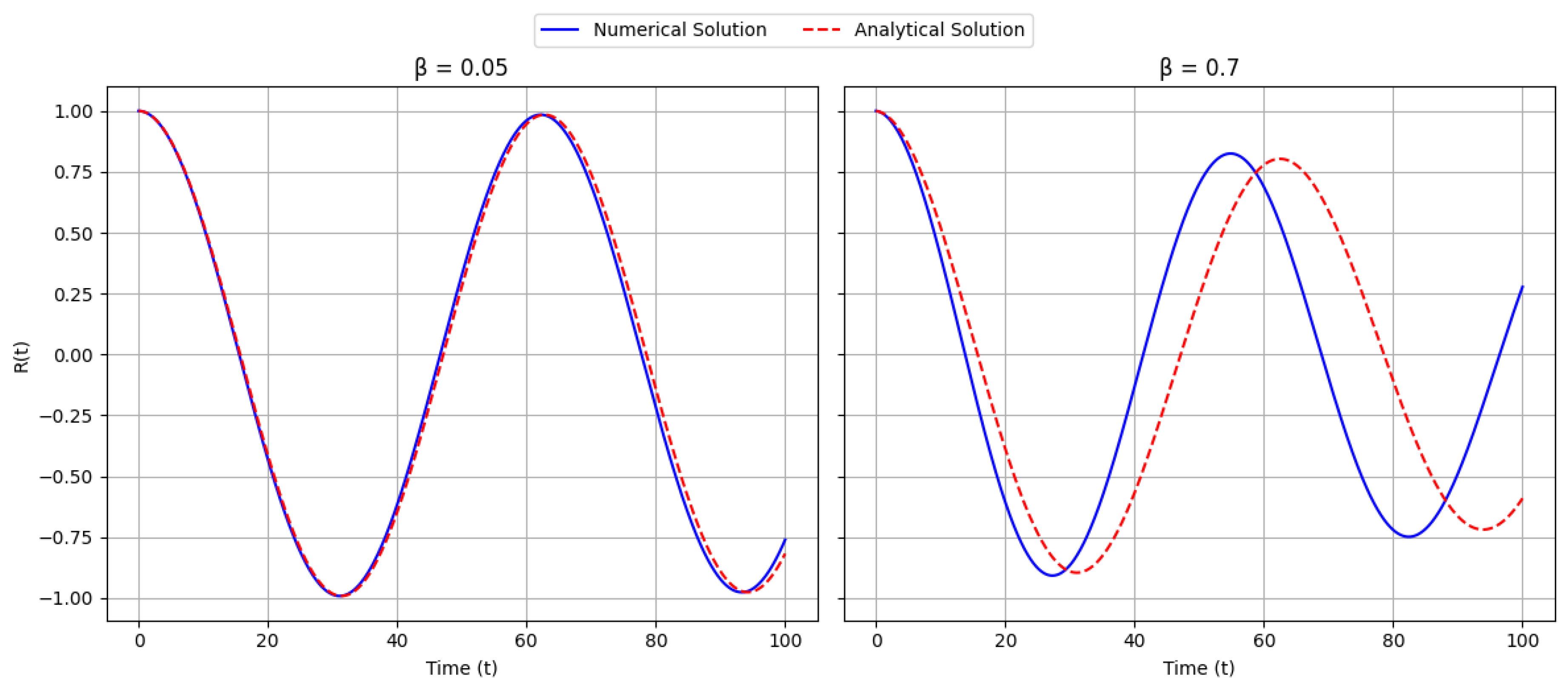
For small values of (e.g., ), the perturbative expansion accurately captures the system’s dynamics. As illustrated in Figure A2, the analytical solution (dashed line) closely follows the numerical solution (solid line) over the entire simulation interval. This excellent agreement confirms that, in the weakly nonlinear regime, the perturbative method yields reliable predictions.
Behavior in the Strongly Nonlinear Regime:
As the nonlinearity parameter increases (e.g., ), discrepancies begin to emerge between the analytical and numerical results. In this regime, the contributions from higher-order nonlinear terms become significant. These discrepancies manifest as phase shifts and amplitude modulations not captured by the first-order perturbative solution. Consequently, the analytical approximation loses accuracy, indicating the need for higher-order corrections to accurately model the system’s behavior.
Fundamental Justification:
The validation process underscores a fundamental principle in perturbation theory: the domain of validity of a perturbative expansion is inherently limited by the magnitude of the nonlinear terms. When the nonlinearity is weak, the leading-order terms dominate, and the analytical solution is robust. However, as the system transitions into a strongly nonlinear regime, neglected higher-order terms begin to influence the dynamics. This behavior is well-documented in nonlinear dynamics literature [2,26,27], and our numerical results corroborate these theoretical expectations.
Figure of Comparison:
Figure A2.
Validation of the analytical solution (dashed line) against numerical results (solid line). For , the agreement is excellent. For larger values of , noticeable discrepancies indicate the need for higher-order corrections.
Figure A2.
Validation of the analytical solution (dashed line) against numerical results (solid line). For , the agreement is excellent. For larger values of , noticeable discrepancies indicate the need for higher-order corrections.
Conclusion:
The validation of the analytical solution against numerical simulations confirms that our perturbative approach is well-suited for capturing the essential dynamics of the system in the weakly nonlinear regime. The observed deviations for larger provide valuable insight into the limitations of the current expansion and highlight the importance of including higher-order corrections for strongly nonlinear behavior. This comprehensive validation not only reinforces the credibility of our analytical methods but also guides future refinements in modeling emergent temporal phenomena in nonlinear gravitational systems.
References
- Einstein, A. (1915). The Field Equations of Gravitation. Sitzungsberichte der Preussischen Akademie der Wissenschaften.
- Strogatz, S. H. (2014). Nonlinear Dynamics and Chaos: With Applications to Physics, Biology, Chemistry, and Engineering. Westview Press.
- Hawking, S., & Penrose, R. (1970). The Singularities of Gravitational Collapse and Cosmology. Proceedings of the Royal Society A, 314, 529–548.
- Carroll, S. M. (2004). Spacetime and Geometry: An Introduction to General Relativity. Addison-Wesley.
- Wald, R. M. (1984). General Relativity. University of Chicago Press.
- Misner, C. W., Thorne, K. S., & Wheeler, J. A. (1973). Gravitation. W. H. Freeman.
- Padmanabhan, T. (2010). Gravitation: Foundations and Frontiers. Cambridge University Press.
- Ashtekar, A., & Singh, P. (2011). Loop Quantum Cosmology: A Status Report. Classical and Quantum Gravity, 28(21), 213001. [CrossRef]
- Bojowald, M. (2008). Quantum Cosmology: A Fundamental Description of the Universe. Springer.
- Ellis, G. F. R., Maartens, R., & MacCallum, M. A. H. (2012). Relativistic Cosmology. Cambridge University Press.
- Penrose, R. (2016). Fashion, Faith, and Fantasy in the New Physics of the Universe. Princeton University Press.
- Kuchař, K. V. (1992). Time and Interpretations of Quantum Gravity. In Proceedings of the 4th Canadian Conference on General Relativity and Relativistic Astrophysics.
- Rovelli, C. (2004). Quantum Gravity. Cambridge University Press.
- Smolin, L. (2001). Three Roads to Quantum Gravity. Basic Books.
- Barbour, J. (1999). The End of Time: The Next Revolution in Physics. Oxford University Press.
- Ashtekar, A., & Singh, P. (2022). Loop Quantum Cosmology: An Overview. Universe, 8(1), 15. [CrossRef]
- Gielen, S., & Turok, N. (2024). Emergent Time and Quantum Cosmology. Physical Review Letters, 132(6), 061302. [CrossRef]
- Brandenberger, R. H. (2021). Beyond Standard Inflationary Cosmology. International Journal of Modern Physics D, 30(14), 2143001. [CrossRef]
- Obied, G., Ooguri, H., Spodyneiko, L., & Vafa, C. (2023). De Sitter Space and the Swampland. Physical Review D, 107(4), 046001. [CrossRef]
- Isham, C. J. (1993). Canonical Quantum Gravity and the Problem of Time. In Integrable Systems, Quantum Groups, and Quantum Field Theories (pp. 157–287). Kluwer Academic Publishers.
- Anderson, E. (2012). Problem of Time in Quantum Gravity. Annalen der Physik, 524(12), 757–786. [CrossRef]
- Kiefer, C. (2012). Quantum Gravity. Oxford University Press, Oxford.
- Rovelli, C. (2018). Forget Time. Foundations of Physics, 48(7), 990–999. [CrossRef]
- Oriti, D. (2014). Group Field Theory and the Emergence of Spacetime. Foundations of Physics, 44(8), 1025–1052. [CrossRef]
- Gielen, S., & Turok, N. (2016). Emergent Spacetime from Quantum Gravity. Physical Review Letters, 116(3), 031301. [CrossRef]
- Nayfeh, A. H. (1973). Introduction to Perturbation Techniques. John Wiley & Sons.
- Kevorkian, J., & Cole, J. D. (1996). Multiple Scale and Singular Perturbation Methods. Springer-Verlag.
- Strogatz, S. H. (2014). Nonlinear Dynamics and Chaos: With Applications to Physics, Biology, Chemistry, and Engineering. Westview Press.
- Carroll, S. M. (2004). Spacetime and Geometry: An Introduction to General Relativity. Addison Wesley.
- Ashtekar, A., & Singh, P. (2011). Loop Quantum Cosmology: A Status Report. Classical and Quantum Gravity, 28(21), 213001. [CrossRef]
- Bojowald, M. (2008). Quantum Cosmology: A Fundamental Description of the Universe. Living Reviews in Relativity, 11(4). [CrossRef]
- Abedi, J., Dykaar, H., & Afshordi, N. (2017). Echoes from the Abyss: Tentative Evidence for Planck-scale Structure at Black Hole Horizons. Physical Review D, 96(8), 082004. [CrossRef]
- Cardoso, V., Franzin, E., & Pani, P. (2016). Is the Gravitational-Wave Ringdown a Probe of the Event Horizon? Physical Review Letters, 116(17), 171101. [CrossRef]
- Planck Collaboration. (2016). Planck 2015 Results. XVI. Isotropy and Statistics of the CMB. Astronomy & Astrophysics, 594, A16. [CrossRef]
- Ade, P. A. R., et al. (2016). Planck 2015 Results. XVI. Isotropy and Statistics of the CMB. Astronomy & Astrophysics, 594, A16. [CrossRef]
Table 1.
Expanded comparison between different theoretical approaches. “Yes” indicates robust features, while “Partial” or “Limited” denote features that are less definitive.
Table 1.
Expanded comparison between different theoretical approaches. “Yes” indicates robust features, while “Partial” or “Limited” denote features that are less definitive.
| Theory | Singularity Regularization | Temporal Anomalies | Emergent Time | Observational Predictions | GR Consistency |
|---|---|---|---|---|---|
| Loop Quantum Gravity | Yes | No | No | Limited (Planck scale effects) | Yes |
| String Theory | Partial | No | No | Limited (extra dimensions, dualities) | Yes |
| Our Model | Yes | Yes | Yes | Yes (e.g., gravitational wave echoes, CMB anomalies) | Yes |
Disclaimer/Publisher’s Note: The statements, opinions and data contained in all publications are solely those of the individual author(s) and contributor(s) and not of MDPI and/or the editor(s). MDPI and/or the editor(s) disclaim responsibility for any injury to people or property resulting from any ideas, methods, instructions or products referred to in the content. |
© 2025 by the authors. Licensee MDPI, Basel, Switzerland. This article is an open access article distributed under the terms and conditions of the Creative Commons Attribution (CC BY) license (http://creativecommons.org/licenses/by/4.0/).
Copyright: This open access article is published under a Creative Commons CC BY 4.0 license, which permit the free download, distribution, and reuse, provided that the author and preprint are cited in any reuse.


