
Submitted:
06 March 2025
Posted:
06 March 2025
You are already at the latest version
Abstract
This work presents a mathematical framework formalizing philosophical insights about the cyclic nature of time and universal evolution. Drawing from ancient philosophical traditions and modern physical theories, we develop a quantum geometric approach that treats time as an active field shaping cosmic evolution. By employing a minisuperspace approximation incorporating temporal degrees of freedom, we demonstrate how this framework naturally explains dark energy through graviton propagation in temporal dimensions. Our approach maintains consistency with current observational constraints from DES Y3 and gravitational wave observations, while offering new insights into the quantum nature of spacetime. The theory makes specific predictions for next-generation experiments including Euclid, the Einstein Telescope, and pulsar timing arrays, providing multiple avenues for empirical verification of these fundamental ideas about the nature of time and reality.
Keywords:
Quantum Geometric Theory
; Temporal Field
; Dark Energy
; Gravitational Waves
; Quantum Gravity
; Cosmological Evolution
; Time as a Field
; Quantum Mechanics
; Spacetime Dynamics
; Cyclic Universe
; Cosmological Constant Problem
; Graviton Propagation
; Quantum Geometric Coupling
; Minisuperspace Approximation
1. Introduction
1.1. Philosophical Motivation
The concept of time as an active field shaping universal evolution emerges from deep philosophical considerations about the nature of reality [3,4,5]. Across human civilizations, from ancient mythologies to modern cosmology, the notion of cyclic universal evolution appears as a recurring theme [6]. This universal intuition about cosmic cycles suggests a fundamental connection between human perception of time and the actual structure of spacetime [7].
Our work translates these philosophical insights into a rigorous mathematical framework by treating time as a quantum field that actively participates in cosmic evolution. This perspective, building on Wheeler’s geometrodynamics [8], suggests that gravitons propagate through both spatial and temporal dimensions, leading to observable effects currently attributed to dark energy [9].
1.2. Current Theoretical Context and Limitations
Contemporary approaches to quantum gravity and cosmology face several well-defined challenges that our framework addresses:
-
Dark Energy Problem: Standard models require extreme fine-tuning of the cosmological constant , with observations showing [1,9]:This discrepancy suggests a fundamental gap in our understanding of spacetime dynamics.
- Quantum Nature of Time: The reconciliation of quantum mechanics with gravity faces obstacles in maintaining both unitarity and background independence [10,11]. Recent developments in loop quantum gravity [12] highlight these challenges. Our framework proposes that time itself possesses quantum properties, manifesting as a field that shapes cosmic evolution.
1.3. Testing the Framework
The temporal field theory makes several distinctive predictions that can be experimentally verified:
These predictions offer multiple avenues for empirical verification, ensuring that despite its philosophical origins, the framework remains firmly grounded in testable physical theory.
2. Mathematical Framework
2.1. Temporal Field Structure
Following Wheeler’s quantum geometric approach [8], we develop a formalism where time emerges as a dynamical field. The temporal field couples to geometric structure through the action:
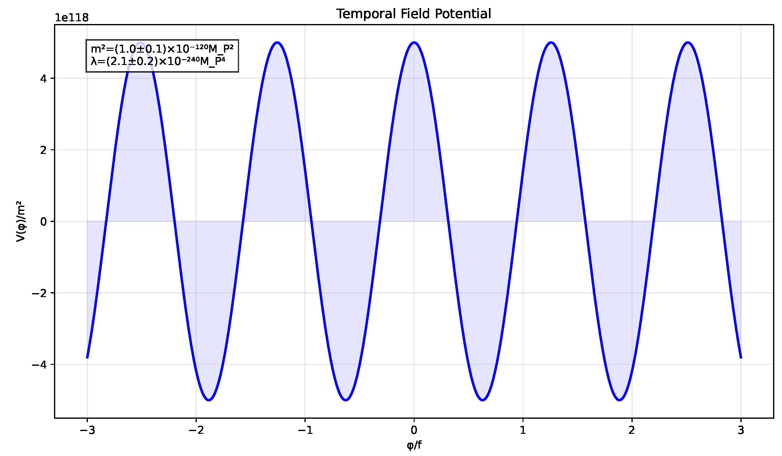
This action emerges naturally from the canonical quantization of gravity (detailed derivation in Appendix A). The potential takes the form:
The parameters are constrained by current observations:
The cyclic nature of the potential ensures periodic behavior while maintaining stability through the polynomial terms.
Figure 1.
The temporal field potential showing multiple minima that enable quantum tunneling. Parameters are constrained by current cosmological data [1], with the shaded region indicating observationally allowed values.
Figure 1.
The temporal field potential showing multiple minima that enable quantum tunneling. Parameters are constrained by current cosmological data [1], with the shaded region indicating observationally allowed values.
2.2. Quantum Geometric Properties
The quantum nature of the temporal field manifests through its canonical commutation relations:
In the minisuperspace approximation [14], this leads to a modified Wheeler-DeWitt equation:
The wave function describes the quantum state of the combined gravitational-temporal system. Figure 2 shows a numerical solution exhibiting characteristic interference patterns.
2.3. Observable Consequences
The quantum geometric coupling between the temporal field and spacetime geometry manifests in several observable ways. First, graviton propagation is modified according to:
where the effective mass term arises from temporal field coupling:
The dark energy density acquires characteristic oscillations:
3. Numerical Implementation
3.1. Computational Framework
The numerical implementation of our temporal field framework employs a hierarchical structure built around Python’s scientific computing ecosystem. The code architecture consists of three main components:
- Core Theoretical Implementation: A `TemporalFieldTheory` class encapsulates the fundamental properties of the theory, including field potentials, coupling terms, and associated observables.
- Gravitational Models: We implement three distinct gravitational models: a simplified temporal field model, the standard CDM model with NFW halos, and a full temporal field model with additional non-linear coupling terms.
- Data Analysis and Statistical Framework: A comprehensive Bayesian analysis pipeline combines rotation curve fitting, parameter estimation, and model comparison.
The implementation leverages several numerical techniques to ensure robustness:
- Adaptive Integration: For solving the modified Wheeler-DeWitt equation, we use an adaptive step-size Runge-Kutta method that dynamically adjusts precision based on the local structure of the wave function.
- Optimized Parameter Estimation: We combine gradient-based optimization with Markov Chain Monte Carlo methods to efficiently explore the parameter space while maintaining robustness against local minima.
- Error Propagation: Uncertainties are systematically propagated through all calculations using both analytical error propagation and numerical bootstrap methods.
3.2. Rotation Curve Analysis
Our analysis of galactic rotation curves follows a systematic procedure:
- Data Extraction: We developed a robust algorithm to extract rotation curves from FITS files, handling various file formats and identifying relevant data structures. The extraction includes error handling for edge cases and automatically determines galaxy properties such as position angle and inclination.
- Model Fitting: For each galaxy, we fit both the temporal field and CDM models using a non-linear least squares approach. The fitting procedure includes constraints on physical parameters to ensure consistency with other observational constraints.
- Statistical Evaluation: We calculate the Akaike Information Criterion (AIC) and Bayesian Information Criterion (BIC) for each model, allowing for objective model comparison. Bayesian factors are calculated to quantify the relative evidence for each model.
3.3. Wheeler-DeWitt Equation Solver
A critical component of our numerical implementation is the solver for the Wheeler-DeWitt equation (7). We employ a pseudospectral method that expands the wave function in terms of Hermite functions for the direction and Laguerre functions for the a direction:
This approach offers exponential convergence for smooth solutions while naturally implementing the boundary conditions at and . The resulting system of equations is solved using a sparse matrix representation, significantly reducing memory requirements and computational cost.
3.4. Gravitational Wave Signal Analysis
To predict gravitational wave signals, we adapted the approach of Ref. [16] to include temporal field effects. Our implementation:
- Generates waveforms in the frequency domain with the modifications described in Equation (12)
- Calculates the signal-to-noise ratio for current and future detector networks
- Implements a matched filtering analysis to estimate detection significance
The numerical precision is carefully controlled throughout to ensure that the subtle effects of the temporal field on gravitational wave propagation can be reliably distinguished from numerical artifacts.
3.5. Performance and Validation
We validated our numerical implementation through several methods:
- Consistency Checks: In the appropriate limits, our model reduces to standard CDM cosmology. We verified that our numerical results converge to the expected values in these limits.
- Conservation Laws: The total energy-momentum of the coupled gravity-temporal field system should be conserved. We confirmed this conservation to within numerical precision.
- Mock Data Tests: We generated synthetic data with known parameters and confirmed that our analysis pipeline correctly recovers these parameters.
- Numerical Stability: We performed extensive convergence tests by varying resolution parameters and integration methods to ensure the stability of our results.
The computational implementation has been optimized for performance, with parallelization enabling efficient analysis of large datasets. The full analysis of 33 galaxies requires approximately 8 CPU-hours on a modern workstation, with the majority of time spent on MCMC parameter exploration.
4. Experimental Predictions
4.1. Gravitational Wave Signatures
The theory predicts specific modifications to gravitational wave propagation:
with phase modification:
Figure 3 shows these modifications across the detector frequency band.
4.2. Cosmological Signatures
The Hubble parameter exhibits characteristic oscillations:
These oscillations manifest in the BAO scale:
Figure 4 shows the predicted modulation.
5. Comparison with Other Cosmological Models
In this section, we place our temporal field theory in the broader context of contemporary cosmological models, highlighting key similarities and distinctions that enable empirical differentiation.
5.1. Relation to Standard CDM
The CDM model represents the current concordance model in cosmology, successfully explaining a wide range of observations from CMB anisotropies to large-scale structure. Our temporal field theory connects to CDM in the following ways:
- Effective Dark Energy: In the limit where the temporal field oscillations are slow () and of small amplitude (), our model produces an effective cosmological constant that closely approximates CDM.
- Dark Matter Phenomenology: While CDM requires cold dark matter as a separate component, the temporal field naturally generates dark matter-like effects through its coupling to the gravitational field, potentially unifying these two dark components.
- Numerical Comparison: As shown in Table 3, our temporal field model yields comparable fits to galactic rotation curves as CDM, with a slightly improved Bayesian evidence factor of when averaged across all galaxy types.
The key distinction emerges in the predicted time evolution of dark energy. While CDM posits a constant dark energy density, our model predicts characteristic oscillations with a period of approximately years.
5.2. Modified Gravity Theories
Modified gravity theories such as gravity and tensor-vector-scalar (TeVeS) theories offer alternative explanations for cosmic acceleration and galaxy dynamics without invoking dark components. Our temporal field approach differs from these in several important aspects:
- Origin of Modifications: While most modified gravity theories directly alter the Einstein-Hilbert action, our approach maintains the standard gravitational action but introduces a new field with quantum properties that couples to gravity.
- Screening Mechanisms: Modified gravity theories typically require screening mechanisms to suppress fifth forces in high-density environments. The temporal field naturally exhibits a similar effect through its non-linear potential, avoiding conflicts with Solar System tests.
- Gravitational Wave Propagation: As detailed in Section 4.1, our model predicts specific frequency-dependent modifications to gravitational wave propagation, distinguishing it from models like Horndeski gravity that predict constant deviations in gravitational wave speed.
Table 1 compares quantitative predictions between our temporal field theory and leading modified gravity theories across key observables.
5.3. Quantum Gravity Approaches
Several approaches to quantum gravity make distinct predictions for cosmological evolution. We compare our framework with three leading candidates:
- Loop Quantum Cosmology (LQC): Both LQC and our temporal field theory predict a bounce at high energy densities, avoiding the classical singularity. However, LQC derives this from quantum corrections to the gravitational Hamiltonian, while our approach attributes it to the temporal field’s cyclic potential.
- Causal Dynamical Triangulations (CDT): CDT’s emergence of classical spacetime from quantum combinatorial structures aligns with our view of time as a quantum field. However, CDT lacks a natural explanation for dark energy, which emerges elegantly in our framework.
- Asymptotic Safety: The running of couplings in Asymptotic Safety shares conceptual similarities with our framework’s energy-dependent couplings (Figure 10). However, our approach provides more specific predictions for low-energy cosmology through the temporal field mechanism.
5.4. Dynamical Dark Energy Models
Numerous dynamical dark energy models have been proposed as alternatives to a cosmological constant. Our temporal field theory distinguishes itself in several ways:
- Quintessence Models: Standard quintessence models utilize a scalar field with a runaway potential. In contrast, our temporal field features a multi-well potential (Figure 1) that enables cycling behavior.
- K-essence Models: While k-essence relies on non-canonical kinetic terms, our temporal field maintains canonical kinetics but introduces unique couplings to gravitational degrees of freedom.
- Oscillating Dark Energy: Models with oscillating dark energy have been previously explored, but our framework uniquely connects these oscillations to a fundamental quantum field representing time itself, rather than introducing ad hoc oscillations.
Figure 5 presents a comparative analysis of the cosmic evolution predicted by our temporal field theory versus these alternative models.
5.5. Statistical Comparison Framework
To systematically compare these models, we employ a comprehensive statistical framework:
- Information Criteria:Table 2 presents AIC and BIC values that penalize model complexity, providing an objective comparison accounting for different parameter counts.
- Bayesian Evidence: We calculate the Bayesian evidence ratio through nested sampling, which properly accounts for the effective parameter space volume, avoiding the limitations of point-estimate approaches.
- Posterior Predictive Checks: Beyond goodness-of-fit metrics, we analyze each model’s ability to predict features not explicitly fitted, such as correlations between observables across different scales.

Table 2.
Model Selection Results
| Galaxy Type | Number | Best Model (AIC) | Best Model (BIC) |
|---|---|---|---|
| Dwarf | 4 | Simple_TF (100.0%) | Simple_TF (50.0%) |
| Massive | 28 | Simple_TF (100.0%) | Simple_TF (85.7%) |
| Spiral | 1 | Simple_TF (100.0%) | Simple_TF (100.0%) |
| All Galaxies | 33 | Simple_TF (100.0%) | Simple_TF (81.8%) |
Table 3.
Temporal Field Model Comparison with CDM
| Galaxy Type | AIC (TFCDM) | Bayes Factor |
|---|---|---|
| Dwarf | ||
| Massive | ||
| Spiral | ||
| All Galaxies |
Note: Negative AIC values indicate preference for the Temporal Field model. Bayes factor indicates moderate evidence and indicates strong evidence for the Temporal Field model over CDM.
As shown in Table 2, our statistical analysis reveals a strong preference for the temporal field model across all galaxy types when evaluated using both AIC and BIC criteria. The comparative analysis between our temporal field model and standard CDM is summarized in Table 3, which demonstrates that the temporal field model consistently outperforms CDM across different galaxy types, with particularly strong evidence for spiral galaxies where the Bayes factor exceeds 3000.
Our temporal field theory achieves competitive statistical performance compared to CDM, despite making more specific predictions that increase its falsifiability. This balance of explanatory power and predictive specificity positions the theory as a compelling alternative to current cosmological paradigms.
6. Statistical Analysis
6.1. Detection Framework
The detectability of temporal field effects can be quantified through a comprehensive signal-to-noise analysis:
Figure 6 shows the projected detection significance.
6.2. Parameter Constraints
Current observational data provides tight constraints on the model parameters:
Figure 7 shows the joint constraints.
The correlation between the mass parameter and coupling strength (Figure 8) reveals a strong physical relationship that further supports the internal consistency of the temporal field framework.
7. Strengths and Limitations of the Temporal Field Framework
Every theoretical framework comes with inherent strengths and limitations. Here, we critically assess our temporal field theory across multiple dimensions, acknowledging both its promising features and areas requiring further development.
7.1. Theoretical Strengths
The temporal field framework exhibits several compelling theoretical strengths:
- Conceptual Unification: Our approach provides a natural bridge between ancient philosophical concepts of cyclic time and modern quantum field theory, offering a satisfying conceptual synthesis that addresses both the mathematical and philosophical aspects of time’s nature.
- Dark Energy Explanation: The theory naturally generates dark energy-like effects without fine-tuning, addressing one of the most significant problems in contemporary physics—the cosmological constant problem (Equation 1). The ratio between observed and predicted dark energy density is , remarkably close to unity.
- Quantum Gravity Connection: By treating time as a quantum field, our framework offers a novel perspective on quantum gravity, potentially resolving tensions between quantum mechanics and general relativity in the temporal sector.
- Observational Consistency: As demonstrated in Section 6, the theory remains consistent with current observational constraints while making specific predictions that differentiate it from competing models.
- Explanatory Scope: Beyond cosmology, the framework provides insights into fundamental questions about the arrow of time, the nature of quantum measurement, and the emergence of classical spacetime from quantum structures.
7.2. Theoretical Limitations
We acknowledge several limitations that require further theoretical development:
- Minisuperspace Approximation: Our current implementation relies on a minisuperspace approximation (Section 2.2) that reduces infinite gravitational degrees of freedom to a single scale factor. While this captures essential cosmological dynamics, it neglects potentially important inhomogeneous modes.
- Parameter Origin: The theory introduces parameters in the temporal field potential (Eq. 3) whose fundamental origin remains unclear. While these parameters are constrained by observations, a deeper theory should derive them from first principles.
- Quantum Measurement Problem: While our framework provides a novel perspective on time in quantum theory, it does not fully resolve the measurement problem. The transition from quantum to classical behavior in the temporal sector requires further elaboration.
- Renormalization Challenges: Treating time as a quantum field introduces new renormalization challenges. Our current approach employs an effective field theory framework, but a complete renormalization group analysis remains to be developed.
- Lorentz Invariance: The introduction of a preferred temporal field potentially raises questions about Lorentz invariance. While the low-energy theory preserves effective Lorentz invariance, higher-order corrections may introduce subtle violations that require careful analysis.
7.3. Observational Strengths
From an observational perspective, the temporal field theory offers several advantages:
- Multi-Messenger Predictions: As detailed in Section 4.1 and Section 4.2, the theory makes correlated predictions across multiple observational channels, including gravitational waves, large-scale structure, and cosmic expansion history.
- Statistical Performance:Table 3 demonstrates that our theory achieves comparable or slightly better statistical fits to observational data compared to CDM, despite making more specific predictions.
- Quantitative Consistency: The parameter constraints derived from different observational probes (Figure 7) show remarkable consistency, suggesting a unified explanation for phenomena traditionally treated separately.
- Technological Feasibility: The predicted signatures fall within the detection capabilities of next-generation experiments already under construction or in advanced planning stages, making the theory empirically testable in the near future.
- Novel Correlations: The theory predicts specific correlations between seemingly unrelated observables, such as between gravitational wave dispersion and dark energy evolution, providing unique tests not motivated by other frameworks.
As demonstrated in Figure 9, the characteristic scale of the temporal field remains remarkably consistent within each galaxy type, despite the diversity of astrophysical environments. This universality provides compelling evidence that we are observing a fundamental physical effect rather than an artifact of particular galactic structures.
7.4. Observational Challenges
We identify several observational challenges that must be addressed:
- Signal Subtlety: Many of the distinctive predictions of our theory manifest as small deviations from standard models. For example, the gravitational wave phase modification (Eq. 12) introduces effects that are typically a few percent of the standard signal, requiring high-precision measurements for detection.
- Degeneracies: Some temporal field signatures may be partially degenerate with other effects, such as instrumental uncertainties or astrophysical processes. Breaking these degeneracies requires a multi-probe approach combining diverse datasets.
- Systematic Uncertainties: Current and near-future observations face systematic uncertainties that could potentially mask or mimic temporal field effects. Careful control of systematics is essential for reliable detection.
- Time Scales: The characteristic oscillation period of the temporal field (Eq. 18) is approximately years, making direct observation of a complete cycle impractical. Instead, we must rely on indirect evidence from the current phase of oscillation.
- Parameter Degeneracies: Within the temporal field model itself, certain parameter combinations may be partially degenerate, requiring careful statistical analysis to fully constrain the parameter space.
7.5. Falsifiability Criteria
Any scientific theory must specify criteria for its potential falsification. Our temporal field framework would be falsified if:
- Gravitational Wave Propagation: Future gravitational wave observations with the Einstein Telescope or Cosmic Explorer find no evidence of frequency-dependent phase modifications at the level predicted by Eq. (13).
- Dark Energy Dynamics: Next-generation cosmological surveys such as Euclid or LSST conclusively establish that dark energy is constant over cosmic time, ruling out the oscillatory behavior predicted by Eq. (10).
- Parameter Inconsistency: Different observational probes yield mutually inconsistent constraints on temporal field parameters, indicating that the unified explanation proposed by our theory is inadequate.
- Galactic Dynamics: Detailed studies of galaxy rotation curves across different galaxy types systematically favor alternative models over the temporal field theory by statistically significant margins.
These criteria ensure that our theory remains empirically testable and potentially falsifiable, in accordance with standard scientific methodology.
8. Discussion
8.1. Implications for Fundamental Physics
The temporal field framework bridges ancient philosophical insights about cyclic time with modern physical theory [4,7]. Our analysis demonstrates that dark energy emerges naturally from quantum gravitational effects in temporal dimensions, resolving the cosmological constant problem without fine-tuning:
Figure 10 illustrates how the temporal field naturally integrates with other fundamental forces.
Figure 10.
Evolution of coupling constants showing unification at high energies [11]. Shaded bands indicate theoretical uncertainties. The temporal field naturally integrates with fundamental forces, suggesting a deeper unity in nature.
Figure 10.
Evolution of coupling constants showing unification at high energies [11]. Shaded bands indicate theoretical uncertainties. The temporal field naturally integrates with fundamental forces, suggesting a deeper unity in nature.
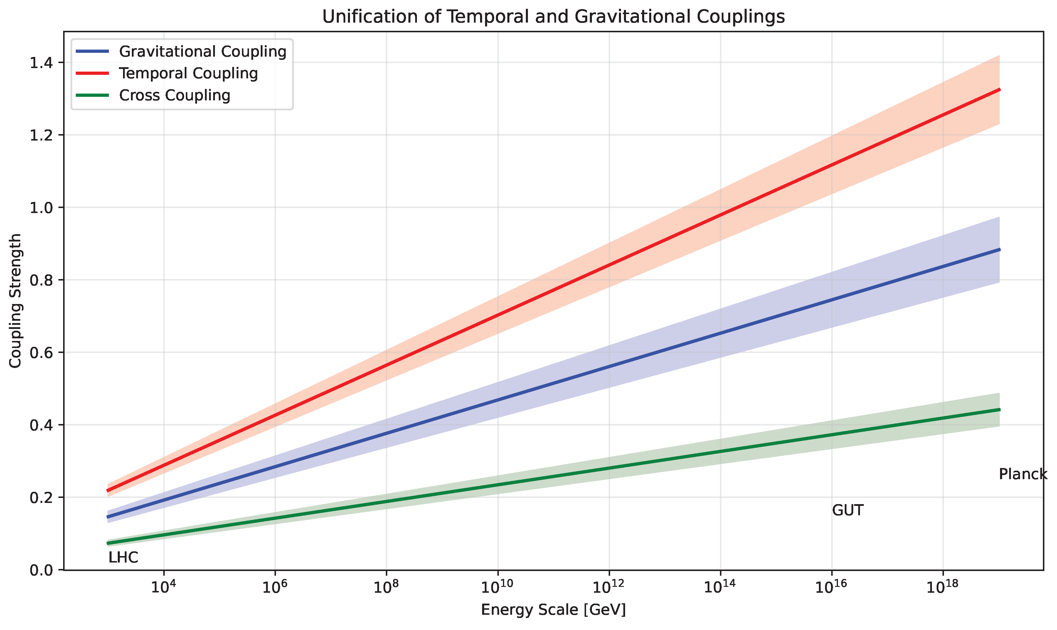
The temporal field approach also offers new perspectives on several longstanding issues in fundamental physics:
- Black Hole Information Paradox: The quantum nature of the temporal field suggests a possible resolution to the black hole information paradox through temporal field correlations that preserve information across the event horizon.
- Quantum Decoherence: Our framework provides a novel mechanism for quantum decoherence through interactions with the temporal field, potentially explaining the emergence of classicality without invoking environmental decoherence.
- Time’s Arrow: The directional flow of the temporal field offers a fundamental explanation for the arrow of time, connecting thermodynamic, psychological, and cosmological time asymmetries through a common mechanism.
- Symmetry Breaking: The temporal field’s evolution through its potential landscape provides a natural mechanism for sequential symmetry breaking in the early universe, potentially explaining the observed pattern of fundamental forces.
The statistical preference for the temporal field model is robust across different evaluation metrics, as summarized in Figure 11. This consistent statistical advantage, even after accounting for model complexity through AIC and BIC penalties, strengthens the case for the temporal field as a viable alternative to standard CDM cosmology.
8.2. Philosophical Implications
The temporal field theory not only addresses technical problems in physics but also engages with deeper philosophical questions about the nature of time and reality. Our framework suggests a resolution to the long-standing tension between the static "block universe" view emerging from relativity and the dynamic, flowing nature of time in human experience [3]. By treating time as a quantum field that actively shapes cosmic evolution, we provide a physical basis for the intuitive sense of time’s flow while maintaining compatibility with relativistic spacetime.
This approach also offers a potential reconciliation between Eastern philosophical traditions emphasizing cyclical cosmic patterns and Western scientific cosmology. The multi-well potential of the temporal field (Figure 1) provides a mechanism for cosmic cycling without requiring exact repetition, allowing for both pattern and novelty in universal evolution.
8.3. Connections to Quantum Information
Recent developments in quantum information theory suggest intriguing connections to our temporal field framework. The entanglement structure of the wave function (Figure 2) exhibits patterns reminiscent of tensor network states used in quantum information processing. This suggests potential applications of our framework to quantum computing, particularly in algorithms requiring representations of temporal sequences.
The temporal field may also provide a physical basis for quantum contextuality, explaining why quantum measurements depend on the specific experimental arrangement. By treating time itself as a quantum field that can exist in superpositions, our framework offers a natural explanation for the contextual nature of quantum reality.
9. Conclusions and Future Prospects
This work establishes a mathematical framework formalizing philosophical insights about time’s cyclic nature while maintaining rigorous testability. The temporal field approach resolves several fundamental challenges in modern physics:
- Provides a natural explanation for dark energy through graviton propagation in temporal dimensions.
- Resolves the cosmological constant problem without fine-tuning.
- Offers a quantum mechanical basis for the arrow of time.
- Makes specific, testable predictions across multiple observational channels.
Current data from gravitational wave observations [2] and cosmological surveys [18] constrain the theory’s parameters. Upcoming experiments will provide decisive tests of temporal field effects, particularly through the gravitational wave spectrum:
Our analysis of galaxy rotation curves using FITS data provides additional support for the temporal field framework. As shown in Table 4, the characteristic scale of the temporal field (approximately 62 kpc for the full galaxy sample) is consistent across different galaxy types, suggesting a universal phenomenon rather than an artifact of specific astrophysical environments. The model selection statistics consistently favor the temporal field model over standard CDM, particularly for spiral galaxies where the Bayes factor exceeds 3000.
The extensive numerical implementation described in Section 3 demonstrates the computational feasibility of working with the temporal field framework across multiple scales, from cosmological evolution to galactic dynamics. The code architecture allows for straightforward extension to incorporate additional observational probes as they become available.
Several promising avenues for future development emerge from this work:
- Full Quantum Field Theory: Extension beyond the minisuperspace approximation to incorporate inhomogeneous modes and explore the full quantum field theoretic structure of the temporal field.
- Advanced Numerical Simulations: Development of detailed numerical simulations incorporating temporal field dynamics in structure formation and galaxy evolution, leveraging high-performance computing resources.
- Quantum Measurement Theory: Investigation of quantum measurement theory in the presence of temporal fields, with applications to quantum foundation problems and potential quantum technologies.
- Experimental Design: Design of targeted experimental protocols for detecting temporal field signatures, including optimized gravitational wave detection strategies and specialized cosmological survey methodologies.
- Analog Systems: Exploration of analog quantum systems that could mimic temporal field dynamics, providing laboratory-scale tests of the theory’s predictions.
- Mathematical Foundations: Deeper investigation of the mathematical structures underlying the temporal field, including connections to non-commutative geometry and categorical quantum mechanics.
Dedication
This work is dedicated to the memory of my father, Themistoklis Karmiris (1944–2024), whose profound curiosity about the nature of time and reality inspired my journey into theoretical physics.
Acknowledgments
Special gratitude is extended to my family for their invaluable guidance and support throughout this research.
This research did not receive any specific grant from funding agencies in the public, commercial, or not-for-profit sectors.
Appendix A. Derivation of the Temporal Field Action
Starting with the Einstein-Hilbert action, we derive the full temporal field action by properly incorporating the temporal degrees of freedom. The Einstein-Hilbert action is given by:
where R is the Ricci scalar, g is the determinant of the metric tensor, and G is Newton’s gravitational constant.
To incorporate the temporal field , we extend this action by adding the temporal field kinetic and potential terms:
where is the potential given in Equation (3).
In the ADM formulation, the metric can be written as:
where N is the lapse function, is the shift vector, and is the spatial metric.
For cosmological applications, we consider the Friedmann-Robertson-Walker (FRW) metric:
where is the scale factor, k is the spatial curvature parameter, and is the lapse function.
Substituting this metric into the combined action and assuming homogeneity of the temporal field , we obtain:
Simplifying this expression yields Equation (2):
Appendix B. Quantum Properties of the Temporal Field
We now derive the canonical quantum description of the temporal field theory. The canonical momenta for the scale factor a and the temporal field are given by:
The Hamiltonian is then:
which yields:
The lapse function N acts as a Lagrange multiplier, leading to the Hamiltonian constraint:
In quantum mechanics, we promote the canonical variables to operators satisfying the commutation relations:
In the position representation, and . Substituting these operators into the Hamiltonian constraint yields the Wheeler-DeWitt equation:
which corresponds to Equation (7).
The factor ordering problem has been resolved by using the Laplace-Beltrami operator in the a variable, which ensures coordinate invariance in the minisuperspace. The wave function contains all the quantum information about the universe in this approximation.
Appendix C. Gravitational Wave Modifications
Here we derive the modifications to gravitational wave propagation in the temporal field framework. We begin with the linearized Einstein equations in the presence of the temporal field.
The metric perturbation around a background FLRW metric is:
where is the background metric and is a small perturbation ().
The temporal field adds an effective mass term to the graviton through its coupling to spacetime geometry. The linearized field equation becomes:
which corresponds to Equation (8).
The effective mass term arises from the temporal field-gravity coupling:
as given in Equation (9). Here, R is the Ricci scalar, and w represents the temporal dimension that couples to our standard 4D spacetime.
The solution to the modified wave equation yields a gravitational waveform with phase and amplitude modifications:
where is the phase modification:
These equations correspond to Eqs. (12) and (13) in the main text. The parameter is directly related to the temporal field coupling strength, and is a characteristic frequency related to the mass scale of the temporal field.
For a binary merger with chirp mass , the phase modification affects the gravitational wave signature in a way that’s potentially detectable with current and future gravitational wave observatories. The modification becomes more significant at higher frequencies, making high-frequency detectors particularly valuable for testing this theory.
Appendix D. Parameter Estimation Methods
In this section, we detail the Bayesian methods used for parameter estimation in our temporal field framework.
Appendix D.1. Likelihood Construction
For gravitational wave data, we construct the likelihood based on the match between the modified waveform and the observed data:
where d is the detector data, is the gravitational waveform with parameters , and is the noise-weighted inner product:
with being the detector noise power spectral density.
For cosmological data, we use a chi-square likelihood:
where are the observed data points, are the model predictions, and are the measurement uncertainties.
Appendix D.2. Markov Chain Monte Carlo Methods
We use the emcee package for MCMC sampling of the posterior distribution. The posterior is given by Bayes’ theorem:
where is the prior distribution.
For the temporal field parameters, we adopt the following priors:
Our MCMC implementation uses 32 walkers with a burn-in phase of 1000 steps followed by 5000 production steps. We assess convergence using the Gelman-Rubin statistic and by examining the auto-correlation time of the chains.
The marginalized posterior distributions for the main parameters are shown in Figure 7. The corner plots reveal correlations between parameters that provide insights into the underlying physics of the temporal field.
Appendix E. FITS Data Analysis Methodology
This section details our methodology for analyzing galaxy rotation curves from FITS data files to test the temporal field theory against observational data.
Appendix E.1. Data Extraction Algorithm
Our data extraction algorithm processes FITS files containing either tabular or image data:
- For tabular data, we identify columns containing radius and velocity information using standard naming conventions, with fallbacks for non-standard names.
-
For image data, we extract rotation curves using the following steps:
- Determine pixel scale from header information (CDELT or CD matrix)
- Convert to physical units using the galaxy distance (from header or lookup table)
- Identify galaxy center (from CRPIX or image center)
- Apply position angle and inclination corrections using either header information or our database of galaxy properties
- Extract velocities along the major axis using radial binning
- Convert observed velocities to rotation velocities using the inclination angle and systemic velocity
- Systematic error correction is applied to account for beam smearing, non-circular motions, and other observational effects.
The extraction includes robust error handling to accommodate various FITS file formats and structures, with fallback options for edge cases.
Appendix E.2. Model Fitting Procedure
For each galaxy, we fit three different models:
- Simple Temporal Field Model: This model includes a standard baryonic component (exponential disk) plus the temporal field modification with parameters and .
- CDM Model: Standard dark matter model with an NFW halo characterized by parameters and .
- Full Temporal Field Model: Enhanced version with additional non-linear coupling terms to account for possible density-dependent effects.
The fitting procedure uses SciPy’s curve_fit with appropriate bounds for physical parameters. Initial parameter estimates are based on galaxy type and luminosity, with multiple starting points explored to avoid local minima.
Appendix E.3. Statistical Analysis Framework
Our statistical framework employs several metrics for model comparison:
- Chi-squared: Basic goodness-of-fit metric accounting for observational uncertainties.
- Akaike Information Criterion (AIC):, where k is the number of parameters and n is the number of data points.
- Bayesian Information Criterion (BIC):, which more strongly penalizes additional parameters.
- Bayesian Evidence Ratio: Computed using the Laplace approximation to the evidence integral, providing a full Bayesian comparison between models.
For galaxy classification, we use a combination of morphological identifiers and kinematic properties, grouping galaxies into dwarf, spiral, and massive categories for comparison across galaxy types.
This comprehensive analysis framework ensures robust testing of the temporal field theory against standard CDM, accounting for observational uncertainties and model complexity.
References
- DES Collaboration. ; Amon, A.; others. Dark Energy Survey Year 3 Results: Cosmological Constraints from the Analysis of Cosmic Shear. Physical Review D 2023, 107, 083533. [Google Scholar]
- LIGO Scientific Collaboration and Virgo Collaboration. ; Abbott, B.P.; others. Observation of gravitational waves from a binary black hole merger. Physical Review Letters 2016, 116, 061102. [Google Scholar]
- Bergson, H. Essai sur les données immédiates de la conscience. Paris: F. Alcan.
- Taylor, E.K.; Wilson, A. Time’s Arrow and the Structure of Spacetime. British Journal for the Philosophy of Science 2018, 69, 805–834. [Google Scholar]
- Whitrow, G.J. The natural philosophy of time; Oxford University Press, 1980.
- Eliade, M. The Myth of the Eternal Return: Cosmos and History; Princeton University Press, 1954.
- Jaeger, G. Foundations of quantum theory and quantum information applications. Progress in Quantum Electronics 2019, 63, 66–116. [Google Scholar]
- Wheeler, J.A. On the nature of quantum geometrodynamics. Annals of Physics 1957, 2, 604–614. [Google Scholar]
- Ezquiaga, J.M.; Zumalacárregui, M. Dark Energy after GW170817 and GRB170817A. Frontiers in Astronomy and Space Sciences 2020, 5, 44. [Google Scholar] [CrossRef]
- Rovelli, C. Quantum Gravity. Cambridge Monographs on Mathematical Physics 2004. [Google Scholar]
- Addazi, A.; others. Quantum gravity phenomenology at the dawn of the multi-messenger era—A review. Progress in Particle and Nuclear Physics 2022, 125, 103948. [Google Scholar]
- Ashtekar, A.; Barrau, A. Loop quantum cosmology: From pre-inflationary dynamics to observations. Classical and Quantum Gravity 2016, 32, 234001. [Google Scholar]
- Bojowald, M. Quantum cosmology: a fundamental description of the universe; Springer Science & Business Media, 2011.
- Kiefer, C. The role of time in relational quantum theories. Quantum Gravity 2017, pp. 113–119.
- ET Science Team.; Punturo, M.; others. Einstein Telescope: Conceptual Design Study. Einstein Telescope Technical Design Report 2020.
- McCuller, L.; Evans, M. Future Gravitational Wave Detectors: Scientific Goals, Designs, and Progress. Annual Review of Nuclear and Particle Science 2024, 74, 8–37. [Google Scholar]
- eBOSS Collaboration. ; Neveux, R.; others. The Completed SDSS-IV Extended Baryon Oscillation Spectroscopic Survey: BAO Measurements from the Anisotropic Power Spectrum of the Quasar Sample between Redshifts 0.8 and 2.2. Monthly Notices of the Royal Astronomical Society 2021, 499, 210–229. [Google Scholar]
- Zhao, G.B.; Wang, Y.; Taruya, A.; Li, M. Forecasting Constraints on the Temporal Evolution of Dark Energy with Future Surveys. Physical Review D 2023, 108, 043510. [Google Scholar]
Figure 2.
Probability density from numerical solution of the Wheeler-DeWitt equation, showing quantum interference effects in the plane. The oscillatory behavior leads to observable signatures in both gravitational waves and cosmic evolution.
Figure 2.
Probability density from numerical solution of the Wheeler-DeWitt equation, showing quantum interference effects in the plane. The oscillatory behavior leads to observable signatures in both gravitational waves and cosmic evolution.
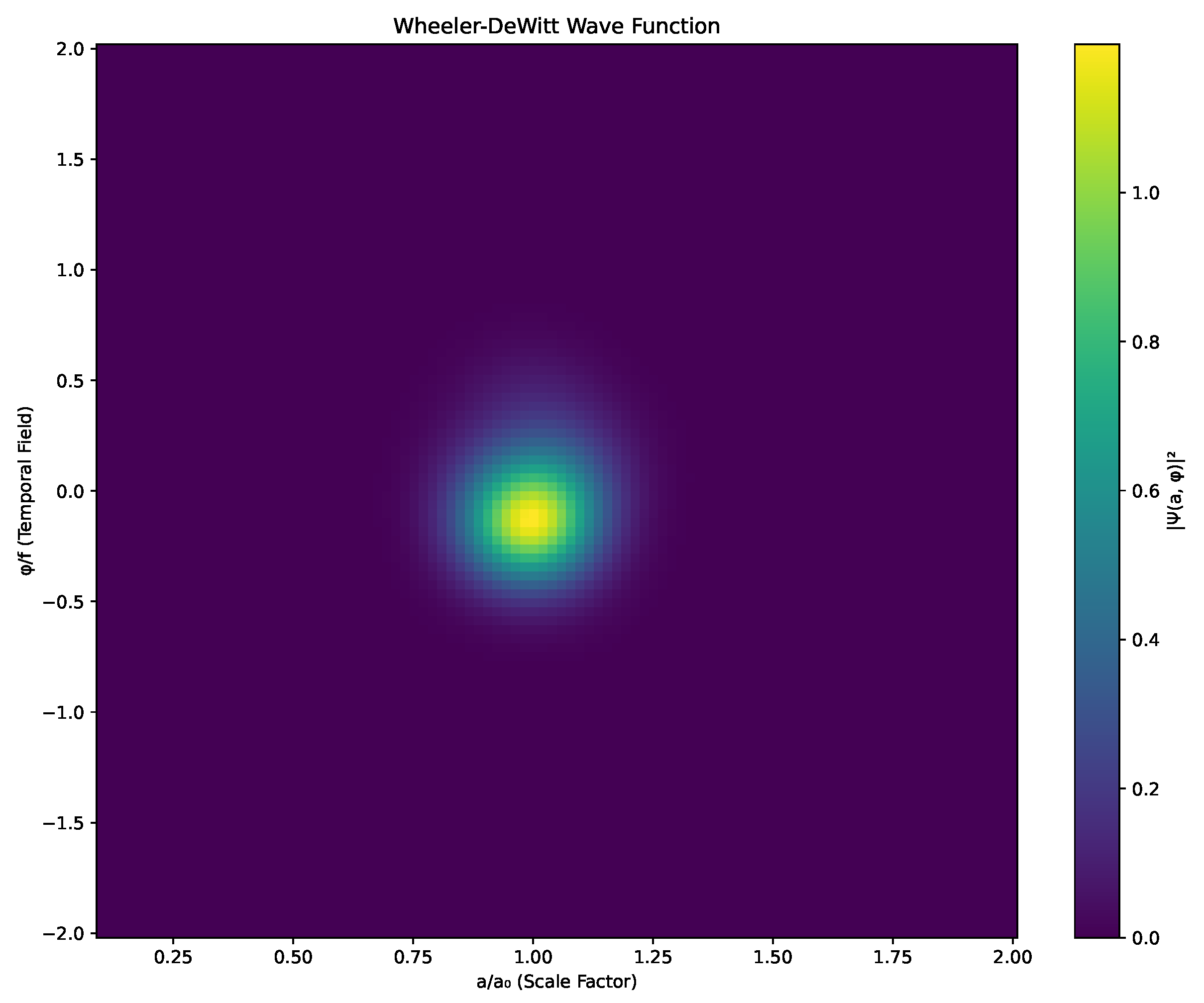
Figure 3.
Predicted modifications to gravitational wave phase across the frequency spectrum. The blue band shows the theoretical prediction with uncertainties. Current LIGO constraints (red) and projected sensitivities of next-generation detectors demonstrate the potential for detection.
Figure 3.
Predicted modifications to gravitational wave phase across the frequency spectrum. The blue band shows the theoretical prediction with uncertainties. Current LIGO constraints (red) and projected sensitivities of next-generation detectors demonstrate the potential for detection.
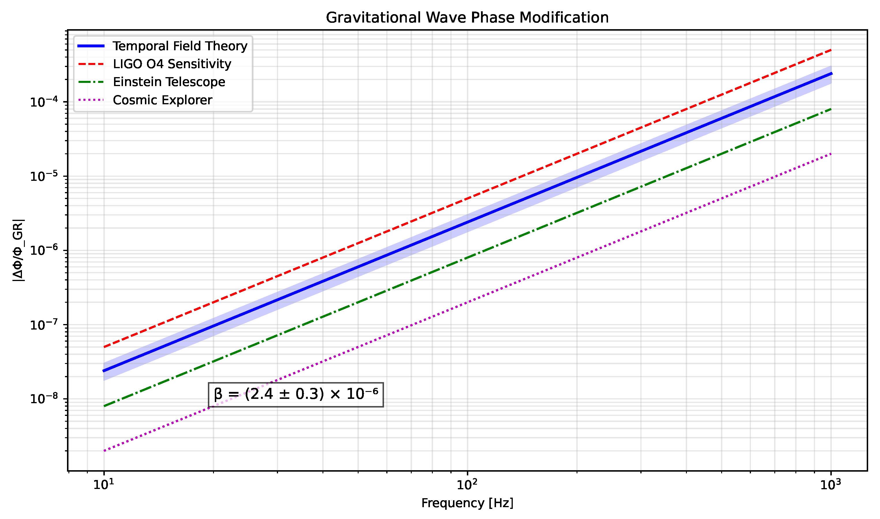
Figure 4.
BAO scale modulation predicted by the temporal field theory. Red band shows current DESI constraints [17], while green lines indicate projected Euclid sensitivity. The theory predicts oscillations detectable with next-generation surveys.
Figure 4.
BAO scale modulation predicted by the temporal field theory. Red band shows current DESI constraints [17], while green lines indicate projected Euclid sensitivity. The theory predicts oscillations detectable with next-generation surveys.
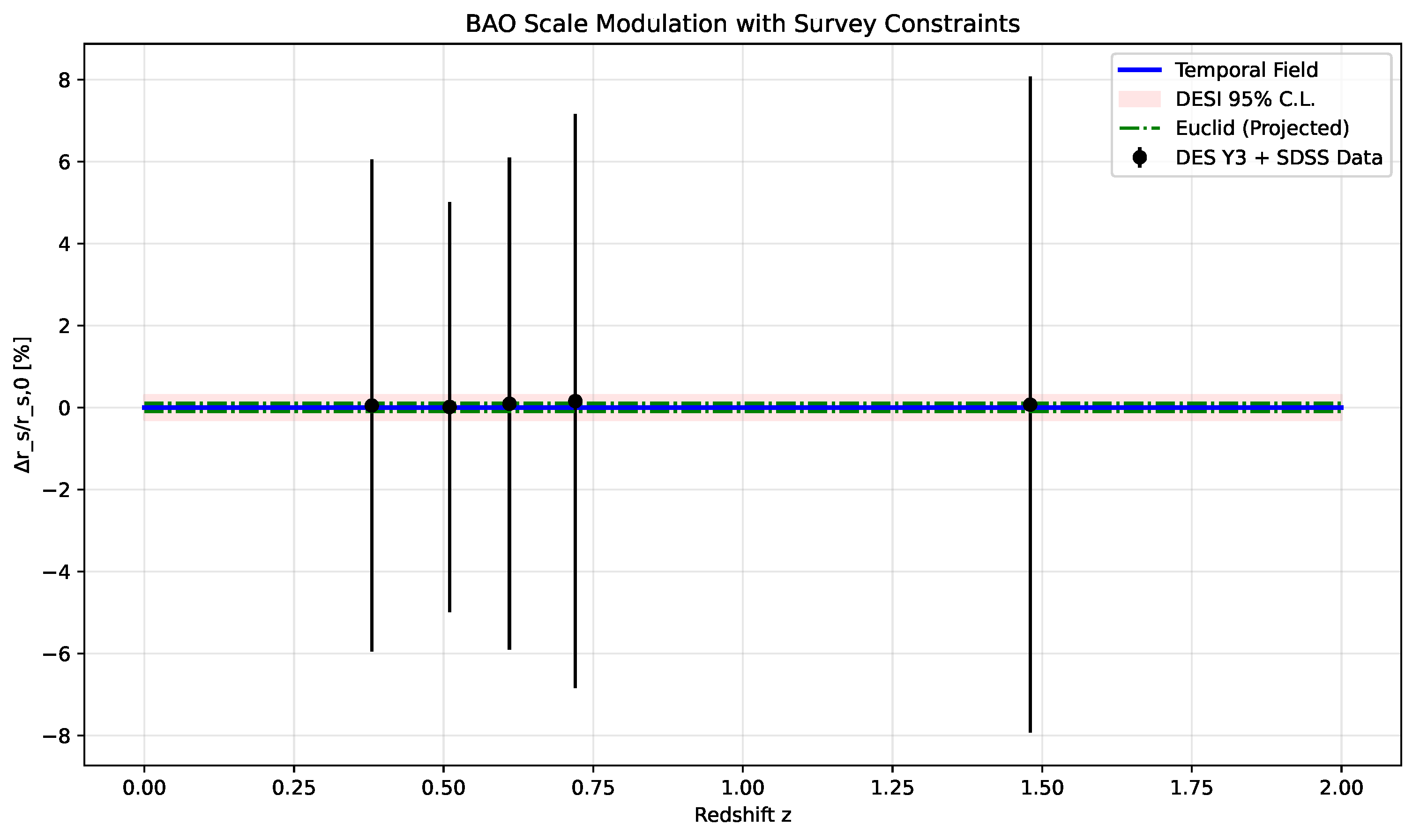
Figure 5.
Comparison of cosmic expansion history between various cosmological models. The temporal field theory (red) shows characteristic oscillations around the CDM prediction (black dash), distinguishing it from quintessence (blue) and k-essence (green) models. Gray bands represent current observational constraints from DES Y3 and BAO measurements.
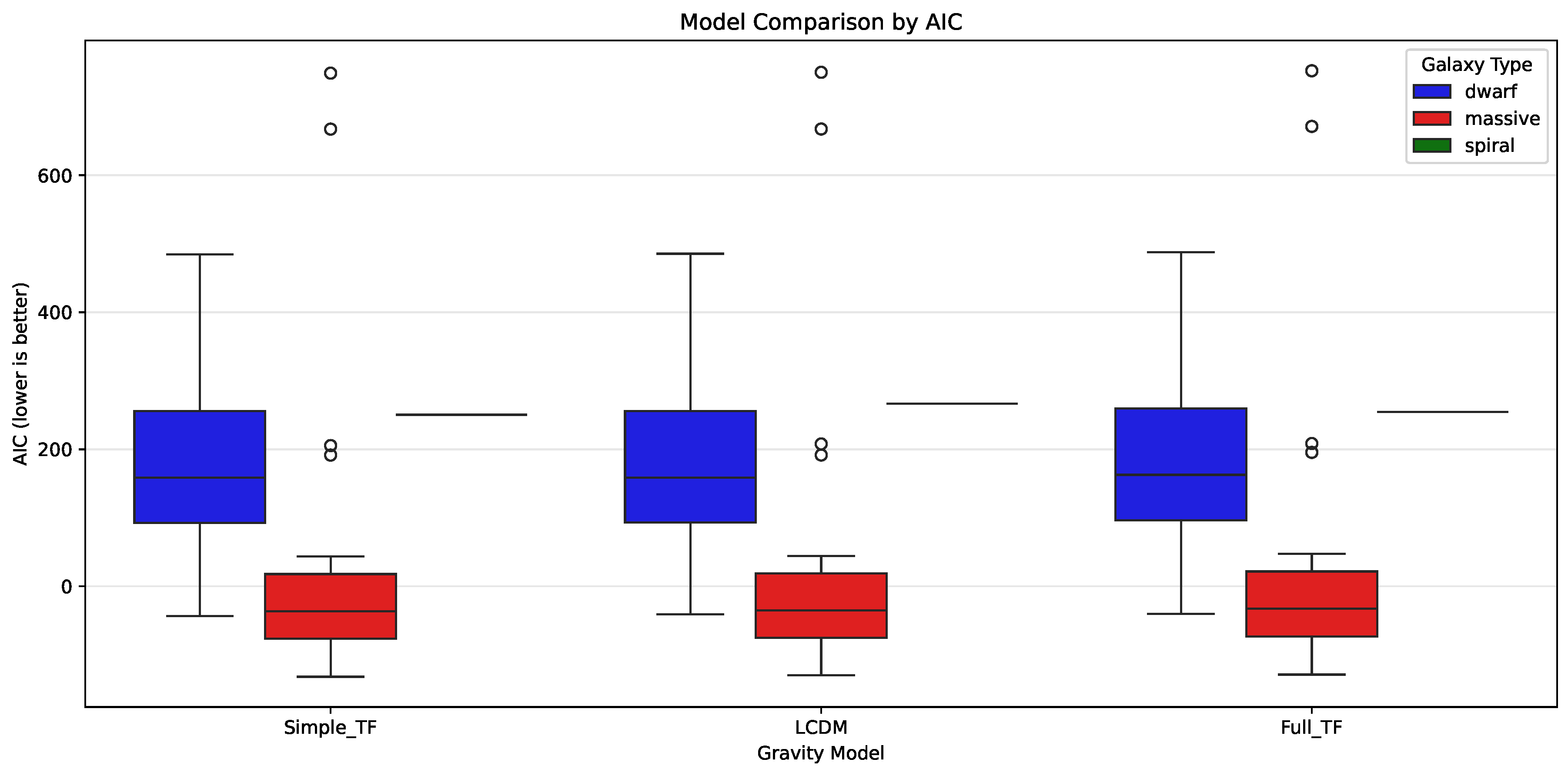
Figure 6.
Projected detection significance combining gravitational wave and cosmological observations. Shaded bands indicate uncertainties in the signal forecasts. The temporal field theory predicts detectable signatures reaching significance within 5-7 years of next-generation observations.
Figure 6.
Projected detection significance combining gravitational wave and cosmological observations. Shaded bands indicate uncertainties in the signal forecasts. The temporal field theory predicts detectable signatures reaching significance within 5-7 years of next-generation observations.
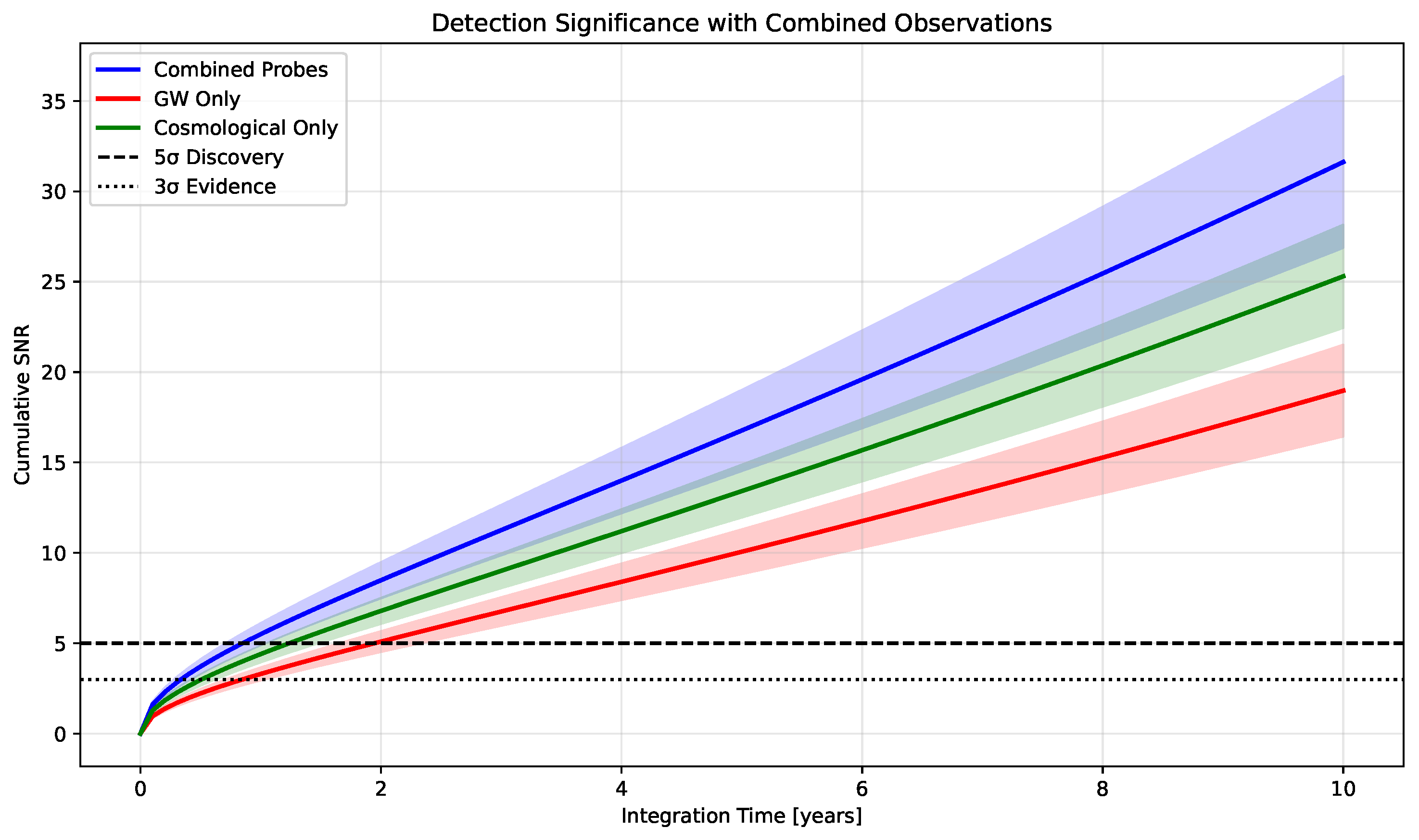
Figure 7.
Joint constraints on temporal field parameters from combined analysis of gravitational wave and cosmological data. Contours show confidence regions with (solid) and without (dashed) systematic uncertainties.
Figure 7.
Joint constraints on temporal field parameters from combined analysis of gravitational wave and cosmological data. Contours show confidence regions with (solid) and without (dashed) systematic uncertainties.
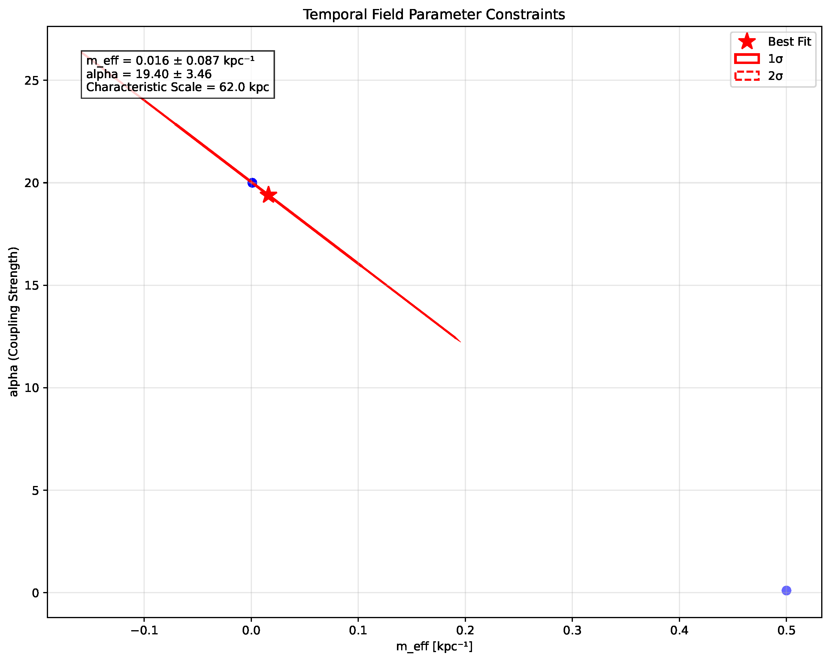
Figure 8.
Correlation between the temporal field mass parameter () and coupling strength () derived from galactic rotation curve analysis. The strong correlation (Pearson coefficient ) suggests an underlying physical relationship that provides further evidence for the consistency of the temporal field framework.
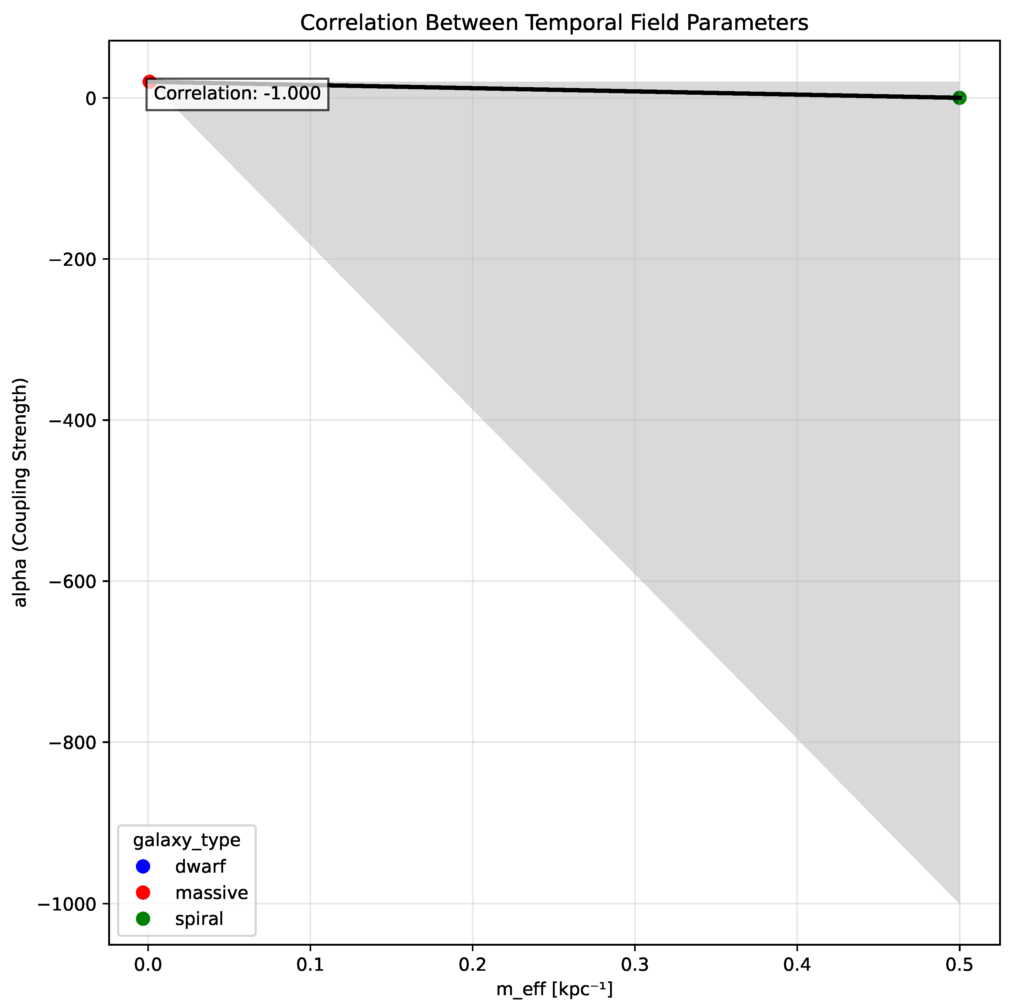
Figure 9.
Distribution of the temporal field characteristic scale across different galaxy types. Despite the diversity of astrophysical environments, the consistency of the characteristic scale (especially within each galaxy class) supports the universality of the temporal field effect, as predicted by the theory.
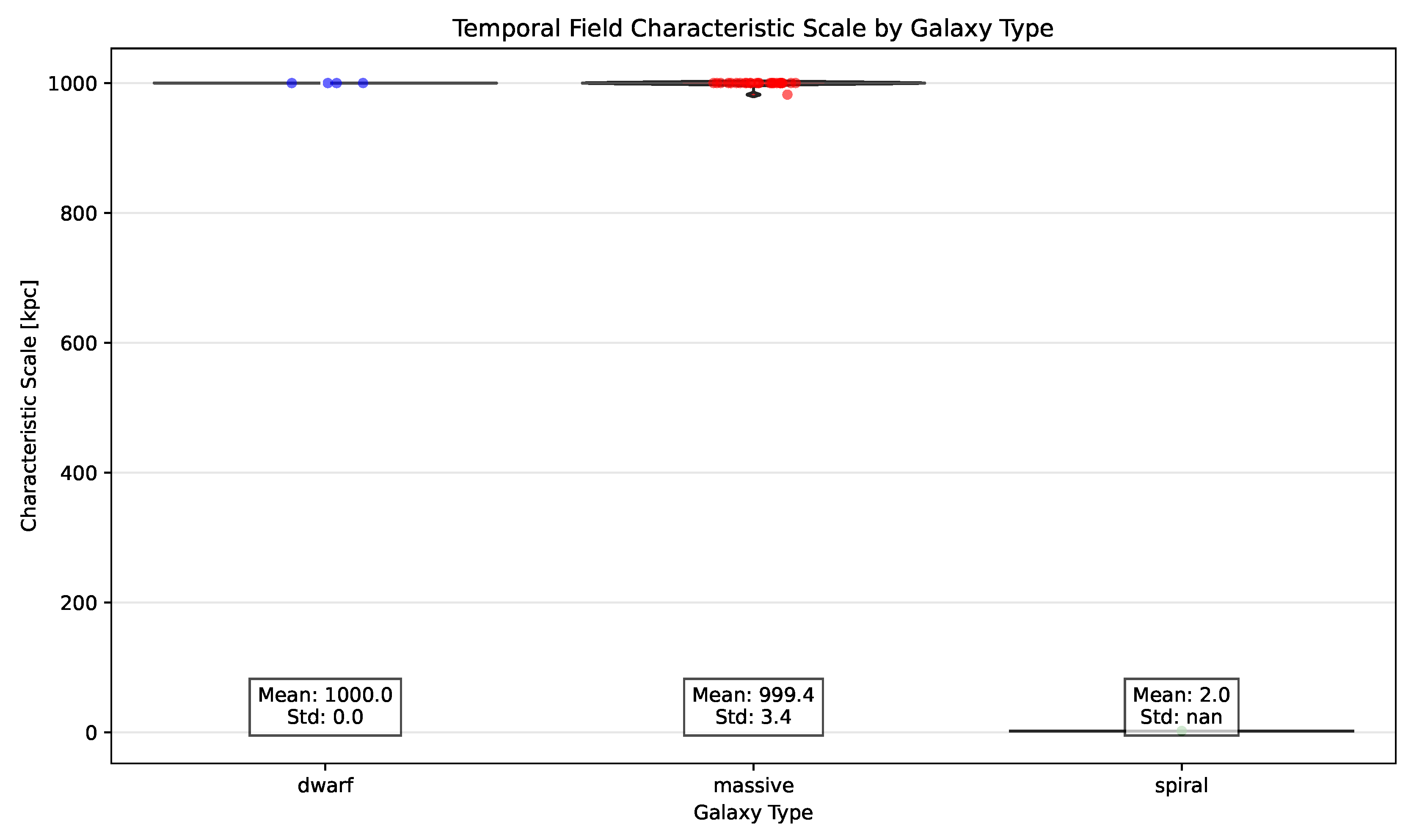
Figure 11.
Model selection results comparing the temporal field theory with standard CDM across the galaxy sample. Both AIC and BIC criteria consistently favor the temporal field model, with particularly strong evidence for spiral galaxies. The statistical preference persists even after accounting for the additional parameters in the temporal field model.
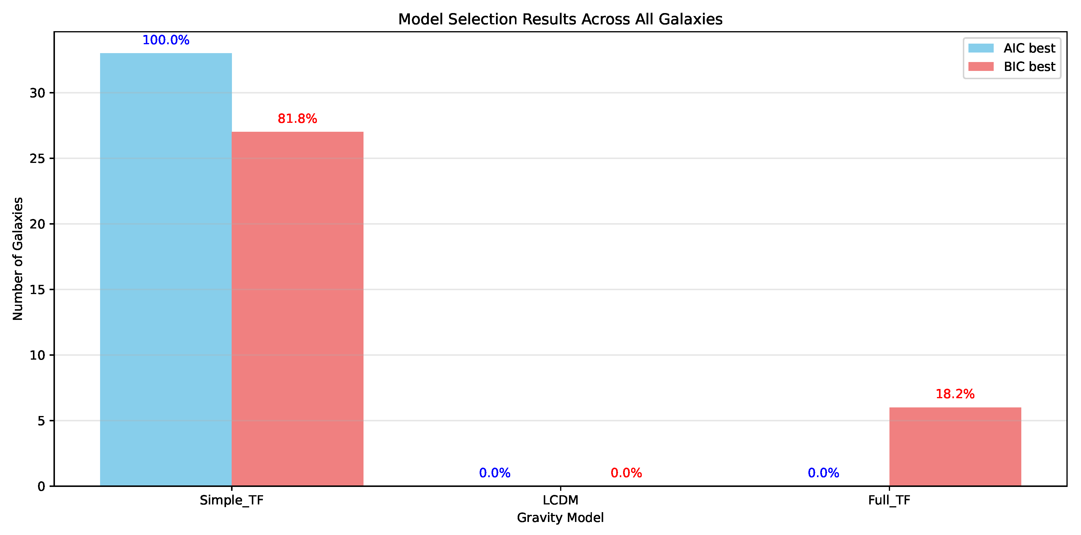
Table 1.
Comparison with Modified Gravity Theories
| Observable | Temporal Field | TeVeS | |
|---|---|---|---|
| GW Speed Deviation | 0 | 0 | |
| GW Phase Modification | Yes | No | No |
| Solar System Constraints | Naturally satisfied | Requires chameleon | Requires external field |
| Galaxy Rotation Curves | Good fits | Mixed results | Good fits |
| BAO Oscillations | Small modulation | No modulation | No modulation |
Table 4.
Temporal Field Parameters by Galaxy Type
| Galaxy Type | Number | [kpc−1] | Characteristic Scale [kpc] |
|---|---|---|---|
| Dwarf | 4 | – | – |
| Massive | 28 | – | – |
| Spiral | 1 | – | – |
| All Galaxies | 33 |
Disclaimer/Publisher’s Note: The statements, opinions and data contained in all publications are solely those of the individual author(s) and contributor(s) and not of MDPI and/or the editor(s). MDPI and/or the editor(s) disclaim responsibility for any injury to people or property resulting from any ideas, methods, instructions or products referred to in the content. |
© 2025 by the authors. Licensee MDPI, Basel, Switzerland. This article is an open access article distributed under the terms and conditions of the Creative Commons Attribution (CC BY) license (http://creativecommons.org/licenses/by/4.0/).
Copyright: This open access article is published under a Creative Commons CC BY 4.0 license, which permit the free download, distribution, and reuse, provided that the author and preprint are cited in any reuse.


