Preprint
Article

This version is not peer-reviewed.

Temporal Dynamics: For Space-Time and Gravity

Submitted:

30 April 2025

Posted:

02 May 2025

You are already at the latest version

Abstract

The concept of space-time has long been a cornerstone of physics, with Einstein’s theory of relativity defining gravity as the curvature of space-time due to mass. However, this research introduces an alternative perspective—Temporal Dynamics, where space remains structurally fixed, and gravity arises from variations in the flow of time. This framework proposes that time flows uniformly through space at a constant rate but is altered by the presence of mass, leading to gravitational effects. By redefining gravity as a consequence of time flow distortions rather than spatial curvature, this model provides new insights into gravitational acceleration, free-fall mechanics, and black hole dynamics. Through derived equations, the study successfully predicts gravitational acceleration for Earth and Mars, demonstrating the framework’s validity. It further explores gravitational lensing, black hole event horizons, and space-time singularities from a temporal flow perspective. The research challenges conventional understandings by suggesting that black holes do not collapse into singularities but instead accumulate mass at the event horizon, where time flow ceases. Additionally, the study introduces the concept of Temporal Dimensions, proposing that variations in time flow could exist as distinct dimensions, influencing our perception of reality. This Temporal Dynamics framework not only aligns with observed gravitational phenomena but also provides an alternative explanation for motion, relativity, and cosmic expansion. By shifting the focus from spatial curvature to time flow variations, this model opens new avenues for understanding gravity, space-time interactions, and potential applications in astrophysics and cosmology.

Keywords: 
;  ;  ;  ;  ;  ;  

Introduction: The Evolution of Space-Time Concepts

Historically, the notion of space as a three-dimensional structure has been fundamental to classical physics, dating back to Euclid and Newton. However, the merging of space and time into a four-dimensional continuum was primarily shaped by the contributions of:
  • Hendrik Lorentz (1890s–1900s) – Developed transformations that suggested time and space are linked.
  • Henri Poincaré (1900s) – Formulated early ideas of relativistic space-time.
  • Albert Einstein (1905, 1915) – Established special and general relativity, demonstrating that time is relative and space-time is curved by mass.
  • Hermann Minkowski (1908) – Introduced the mathematical formalism of space-time as a four-dimensional construct.
While Einstein’s equations successfully explain gravitational interactions, cosmic expansion, and relativistic effects, this paper seeks to explore an alternative view that could provide fresh insights into space-time dynamics.

The Core Premise: A Fixed Space with Dynamic Time Flow

In this alternative model, space is treated as a fixed unit—not in terms of absolute quantity but in terms of its structural existence. To visualize this, consider a road: while the total distance remains fixed at any given moment, additional road can be constructed, expanding its length. Similarly, space expands continuously, not at the edges, but throughout all points simultaneously.
A fundamental assumption in this model is that time moves through space at a uniform rate of 299,792,458 meters per second. This means that at every point in space, time is propagating at this exact speed, giving rise to the “Normal Time Flow.”
Mathematically, the interaction between space and time can be expressed as:
Universal Constant = Unit of Time × Unit of Space Expanded in that Time
U = 1 sec ÷ 299,792,458 m
U = 3.33564095 × 10⁻⁹ s/m
This value, 3.33564095 × 10⁻⁹ s/m, represents a fundamental property of space-time within this framework and remains constant across all locations in the absence of additional influences.

Beyond Uniformity: The Role of Mass and Chaos

If time flowed uniformly through every point in space with an entropy of zero, the universe would be a static and predictable environment. However, the observed universe is far from orderly—mass, energy, and fundamental forces create dynamism and complexity.
In Einstein’s model, mass curves space-time, leading to gravitational attraction. The question this framework now faces is: how does mass interact with time in this model? If space itself remains structurally fixed and expands uniformly, then does mass create a disturbance in time flow instead of bending space? What new interpretations arise from this perspective?
This discussion leads to the next phase of this research: exploring how mass influences the temporal dynamics of this proposed space-time model.

The Nature of Mass in This Model

To understand mass within this alternative framework, consider a straight-line distance from point A to point B. If this distance were to be extended into a curve, its total length would increase. In Einstein’s space-time model, mass curves space, effectively increasing the path an object must travel. However, in this model, mass does not geometrically bend space but instead slows the flow of time within a defined distance.
Since time and space are interconnected, an increase in the time required for light (or any signal) to traverse a specific distance effectively mirrors the effect of an increased spatial path in Einstein’s model, but from a different foundational principle.
Thus, mass does not alter the spatial structure itself but instead modifies the rate of time flow through that space.

The Equation for Additional Time Introduced by Mass

In this framework, mass is responsible for introducing additional time (Δtime) to the Normal Time Flow within a given spatial region. This additional time can be expressed mathematically as:
∆T = (M×Cm) ÷ D
-
∆T= Additional time delay due to mass (s).
-
M = Mass of the object (kg).
-
Cm = Mass constant (2.970330587876230×10^-27 smkg^-1).
Where:
-
D = Distance influenced by mass (m).
This equation is derived from the observed magnitude of mass and its effects on gravitational time dilation. It suggests that as mass increases within a given space, it proportionally increases the additional time experienced in that region. However, this effect is inversely proportional to distance—meaning the farther one moves from the mass, the less time is added to the Normal Time Flow.

Total Time Flow in the Presence of Mass

To determine the actual time flow through a given distance under the influence of mass, we sum the additional time with the Normal Time Flow:
T_mass flow = ∆t + (D × U)
And the normal time flow in the absence of mass is:
T_normal = D × U
Thus, the gravitational ratio, which compares normal time flow to time flow under mass influence, is:
G_ratio = T_normal ÷ T_mass flow
T_actual or T_mass flow = T_normal + ∆T
Where:
T_actual = Actual time flow through the specified distance
T_normal = Normal Time Flow without mass influence, given by:
T_normal = D × U
(Where U is the Universal Constant: 3.33564095 × 10⁻⁹ s/m)
Thus, under the influence of mass, the flow of time slows down relative to what would be expected in a vacuum. This slowing of time is what produces gravitational effects in this model.

Gravity as a Consequence of Time Flow Variations

In this framework, gravity arises not from a curvature in space-time, but from gradients in time flow across different spatial points. When an object moves from a region of faster time flow to a region of slower time flow (closer to a massive object), it experiences an acceleration—akin to falling in a gravitational field.
In Einstein’s model, gravity is a result of space-time curvature.
In this model, gravity results from time gradients—where regions with greater mass introduce slower time flow, creating a “pull” toward them.
This interpretation maintains consistency with observed gravitational time dilation effects but reframes the fundamental cause.

Next Steps: Motion in a Time-Based Gravity Model

Before fully addressing gravity and the derivation of the mass constant (Cₘ), the next step is to explore what causes motion in this model. Since variations in time flow appear to govern gravitational effects, we must first understand how time flow influences movement and acceleration in this framework.

Motion as a Consequence of Time Flow Changes

In this framework, space expands equally in all directions from any point at a rate of 299,792,458 meters per second (speed of light). When a body is in motion, the space in its direction of movement expands more, and the space in the opposite direction expands less. This means that time flows slower in the direction of motion and faster in the opposite direction.
The total distance in the direction of motion after one second is given by:
D_motion = D_expanded + v
Where:
  • D_motion = Total distance expanded in the direction of motion after one second
  • D_expanded = Distance expanded due to normal time flow (299,792,458 m)
  • V = Speed of the moving body
Similarly, in the opposite direction of motion, the total expanded distance is:
D_opposite = D_expanded – v
However, space itself does not change—only the way time flows through it. Since time flow increases in the direction opposite to motion, we can calculate the magnitude of this change in time flow using the ratio of the normal time flow to the altered time flow:
V = ( T_normal ÷ T_altered ) × D_expanded
Since we want to extract only the speed and remove the speed of light from the equation, we refine this to:
V = c - ( T_normal ÷ T_altered × D_expanded)
Where:
  • C = Speed of light (299,792,458 m/s)
  • T_normal = Time flow in absence of motion
  • T_altered = Time flow altered by motion
This equation shows that motion itself is a result of time flow slowing down in the direction of movement, effectively pulling the object forward.

How Gravity and Motion Are Connected

Gravity as a Continuous Time Flow Alteration

In mechanical motion, the time flow changes once due to a force (e.g., a kick transferring energy to a football). The speed is determined by the initial ratio of normal time flow to altered time flow.
In gravitational motion, the time flow continuously changes due to the mass’s persistent influence, meaning that an object’s motion keeps accelerating.
To see this effect, consider that gravitational time flow alters again and again:
  • If normal time flow slows by a factor of 2, the altered time flow becomes ½ of normal time.
  • If it slows further by a factor of 2, it becomes ¼ of the original time flow.
  • If it slows again, it becomes ⅛, then ¹/¹⁶, then ¹/32…
This recursive slowing of time is what causes gravitational acceleration.

The Gravitational Acceleration Equation

Since gravitational acceleration is also caused by a time flow gradient (but continuously applied), we derive:
A = c – (gravitational ratio × D_expanded)
Where:
  • A = Gravitational acceleration
  • C = Speed of light (299,792,458 m/s)
  • Gravitational ratio = Ratio between normal time flow and actual time flow under gravity
This equation suggests that gravitational acceleration is fundamentally the same as motion but with continuously altering time flow, making objects accelerate rather than move at a constant speed.

Conclusion and Next Steps

  • Motion occurs because time flows slower in the direction of movement, creating an effect similar to a “pull” forward.
  • Gravity is essentially the same process but happens continuously, leading to acceleration rather than a constant velocity.
  • This means both motion and gravity are consequences of time flow variations rather than space curvature.
The next step is to apply this model to real-world examples, such as planetary orbits and free-fall motion, to test whether this framework produces the same predictions as Newtonian gravity and General Relativity.

Real-World Applications

Key Theoretical Equations and Their Meaning

Fundamental Equations Relating Mass, Time, and Gravity.
Mass contributes additional time to a given space:
∆ t = (M × C_m) ÷ D
  • M = Mass (kg)
  • C_m = Mass constant (2.970330587876230 × 10⁻²⁷ smkg⁻¹)
  • D = Distance (m)
Total time flow at a distance due to mass:
T_mass flow = ∆ t + (D × U)
D × U = Normal time flow
Gravitational Ratio:
G_ratio = T_normal ÷ T_mass flow
Gravitational Acceleration:
G = c – (g_ratio × D_expanded)
D_expanded = Distance expanded in one second (299,792,458 m)
Alternative Expression for the Gravitational Ratio:
G_ratio = (c – g) ÷ D_expanded

Applying the Framework to Real-World Cases

Case Study 1: Earth’s Gravity
We apply the framework to derive Earth’s gravitational acceleration (9.81 ms²) using known values.
  • Step 1: Calculate the Additional Time Flow Due to Earth’s Mass
    • ∆ t = (5.972 × 10^24) × (2.970330587876230 × 10^-27) ÷ 12,742,000
    • ∆ t = 1.773 × 10^-2 ÷ 12,742,000
    • ∆ t ≈ 1.3908 × 10^-9 s
  • Step 2: Compute the Total Time Flow of Space Influenced by Earth
    • T_mass flow = ∆ t + (D × U)
    • T_mass flow = 1.3908 × 10^-9 + (12,742,000 × 3.33564095 × 10^-9)
    • T_mass flow = 1.3908 × 10^-9 + 0.04250273698
    • T_mass flow ≈ 0.04250273837 s
  • Step 3: Compute the Gravitational Ratio
    • G_ratio = 0.04250273698 ÷ 0.04250273837
    • G_ratio ≈ 0.9999999673
  • Step 4: Compute Earth’s Gravitational Acceleration
    • G = c – (g_ratio × D_expanded)
    • G = 299,792,458 – (0.9999999673 × 299,792,458)
    • G b>G ≈ 9.81 ms²
This matches the known gravitational acceleration on Earth’s surface.

Case Study 2: Mars’ Gravity

  • Step 1: Calculate Additional Time Flow Due to Mars’ Mass
    • ∆ t = (6.4171 × 10^23) × (2.970330587876230 × 10^-27) ÷ 6,792,000
    • ∆ t ≈ 2.805 × 10^-10 s ]
  • Step 2: Compute Mars’ Total Time Flow
    • T_mass flow = 2.805 × 10^-10 + (6,792,000 × 3.33564095 × 10^-9)
    • T_mass flow = 2.805 × 10^-10 + 0.02265
    • T_mass flow ≈ 0.0226500003 s
  • Step 3: Compute Mars’ Gravitational Ratio
    • G_ratio = 0.02265 ÷ 0.0226500003
    • G_ratio ≈ 0.9999999876
  • Step 4: Compute Mars’ Gravitational Acceleration
    • G = 299,792,458 – (0.9999999876 × 299,792,458)
    • G b>G ≈ 3.7 ms²
This matches the known surface gravity of Mars (3.7 ms²).

Conclusion

This research proposes that gravity is not due to space curvature but instead due to variations in time flow caused by mass. The equations derived successfully predict real-world gravitational accelerations for Earth and Mars, supporting the validity of this approach.
Key Takeaways:
  • Mass slows time flow, creating gravitational attraction.
  • Motion occurs due to changes in time flow gradients.
  • Gravitational acceleration is derived purely from time flow alterations.

Derivation of the Mass Constant (Cₘ) in the Temporal Dynamics Framework

The mass constant (Cₘ) is a fundamental parameter in this alternative framework of space-time, where mass influences time flow rather than curving space. It relates mass, time flow distortions, and distance. The derivation of Cₘ is based on the relationship between gravitational acceleration, time flow distortion, and mass distribution.
Step 1: Define the Relationship Between Mass, Time, and Distance
The foundational equation of this framework states that mass contributes an additional time component Δt to a given distance, which in turn affects time flow and causes gravity.
∆ t = M × C_m ÷ D
Where:
  • Δt = Additional time flow distortion due to mass (s)
  • M = Mass of the object (kg)
  • Cₘ = Mass constant (smkg⁻¹)
  • D = Distance influenced by mass (m) (e.g., the diameter of a planet)
The additional time distortion Δt affects the normal time flow, which then determines gravitational acceleration.
Step 2: Establish the Gravitational Acceleration Equation
The gravitational acceleration in this model is given by:
G = c – (g_ratio × D_expanded)
Where:
  • G = Gravitational acceleration (ms²)
  • C = Speed of light (299,792,458 m/s)
  • G_ratio = Gravitational ratio, defined as:
  • G_ratio = T_normal ÷ T_mass flow
  • D_expanded = Distance expanded by space in one second (299,792,458 m)
Since g_ratio depends on Δt, we substitute T_mass flow:
T_mass flow = T_normal + ∆ t
G_ratio = T_normal ÷ (T_normal + ∆ t)
Using the equation for Δt from Step 1:
G_ratio = T_normal ÷ [T_normal + (M × C_m ÷ D)]
This equation directly relates mass to gravitational acceleration.
  • Step 3: Solve for the Mass Constant (Cₘ)
    • We apply this equation to Earth, using known values:
    • Mass of Earth (Mₑ) = 5.972 × 10²⁴ kg
    • Diameter of Earth (Dₑ) = 12,742,000 m
    • Gravitational acceleration (gₑ) = 9.81 ms²
    • Speed of light (c) = 299,792,458 m/s
    • Total distance expanded after 1 second (D_expanded) = 299,792,458 m
    • First, solve for g_ratio:
    • G_ratio = (c – g) ÷ D_expanded
    • G_ratio = (299,792,458 – 9.81) ÷ 299,792,458
    • G_ratio ≈ 0.9999999673
    • Using the definition of g_ratio:
    • G_ratio = T_normal ÷ T_normal + ∆ t
    • Rearrange for Δt:
    • ∆ t = T_normal ÷ g_ratio – T_normal
    • ∆ t = (0.04250273698 ÷ 0.9999999673) – 0.04250273698
    • ∆ t ≈ 1.3908 × 10^-9 s
    • Now, solve for Cₘ using:
    • Mₑ × C_m ÷ Dₑ = ∆ t
    • C_m =( ∆ t × Dₑ) ÷ Mₑ
    • C_m = (1.3908 × 10^-9) × (12,742,000)÷(5.972 × 10^24)
    • C_m ≈ 2.970330587876230 × 10^-27 s m kg^-1
  • Step 4: Validate with Other Celestial Bodies (Mars)
    • For Mars:
    • Mass of Mars (Mₘ) = 6.4171 × 10²³ kg
    • Diameter of Mars (Dₘ) = 6,792,000 m
    • Gravitational acceleration (gₘ) = 3.7 ms²
    • Following the same process, we calculate:
    • G_ratio ≈ 0.9999999876
    • ∆ t ≈ 2.805 × 10^-10 s
    • C_m = (2.805 × 10^-10) × (6,792,000) ÷ (6.4171 × 10^23)
    • C_m ≈ 2.970330587876230 × 10^-27 s m kg^-1
This confirms that Cₘ is consistent across different celestial bodies.

Conclusion

  • The mass constant (Cₘ) was derived using:
  • The relationship between mass, time flow, and distance.
  • Empirical validation using Earth’s and Mars’ known gravitational acceleration.
  • Consistency across different planetary bodies.
  • Final Derived Value of the Mass Constant:
C_m ≈ 2.970330587876230 × 10^-27 s m kg^-1

Explaining Why Bodies of Different Mass Fall at the Same Rate Using the Temporal Dynamics Framework

In classical physics, Galileo’s principle of universal free fall states that all objects, regardless of mass, fall at the same rate in a given gravitational field (neglecting air resistance). Newton’s laws and Einstein’s General Relativity confirm this by showing that gravitational acceleration is independent of an object’s mass.
In this Temporal Dynamics Framework, where gravity results from variations in time flow rather than space curvature, the reason why all objects fall at the same rate becomes even clearer. Instead of considering gravity as a force pulling objects downward, we see it as a response to the rate of time flow at different heights.
Fundamental Premise: Gravity as Time Flow Variation
In this model, mass does not bend space but slows down the flow of time in its vicinity. The gravitational acceleration g at the Earth’s surface is given by:
G = c – (g_ratio × D_expanded)
Where:
  • C = Speed of light
  • G_ratio = Ratio of normal time flow to time flow altered by Earth’s mass
  • D_expanded = Distance space expands in one second (299,792,458 m)
This means that the gravitational acceleration at any point is purely a function of the time flow rate in that region.

Why Mass Doesn’t Affect Free Fall in This Model

When an object is placed in a gravitational field, it experiences the same local time flow variation as any other object at that position.
The mass of the object itself does not contribute to altering time flow significantly, because the dominant time flow effect comes from the mass of the Earth.
Since all objects exist within the same time flow gradient, they are affected equally, independent of their mass.

Mathematical Explanation

In this framework, an object’s speed in free fall is determined by the gravitational acceleration equation:
G = c − (g_ratio × D_expanded)
Since g_ratio depends only on Earth’s mass and diameter, not the object’s mass, g remains the same for all objects.
If object A has a mass of 1 kg and object B has a mass of 100 kg, they both experience the same time flow distortion at a given height.
Because they both move in response to the same time flow gradient, their falling speed is the same.
This directly explains why objects of different masses fall at the same rate.

Comparison with Einstein’s Model

In General Relativity, free fall occurs because objects move along geodesics in curved space-time. Mass does not affect free fall because acceleration due to gravity is a result of space-time curvature rather than the object’s inertia.
In this model, free fall occurs because all objects experience the same time flow distortion at a given location, meaning they adjust their motion according to the same time flow gradient.
Both models predict the same result, but this framework removes the need for space curvature, explaining gravity purely as a function of time flow rates.

Experimental Validation: The Apollo 15 Hammer-Feather Test

During the Apollo 15 Moon mission, astronaut David Scott dropped a hammer and a feather simultaneously in the absence of air resistance. They hit the ground at the same time, confirming that gravitational acceleration is independent of mass.
In this model:
  • The hammer and feather both exist within the same time flow gradient created by the Moon’s mass.
  • Since gravity is just a function of time flow variation, both objects move at the same rate, regardless of their different masses.
  • The experimental results are naturally explained by this framework.

Conclusion

In this Temporal Dynamics Framework:
  • Gravity is not a force, but a response to gradients in time flow.
  • All objects in the same time flow gradient experience the same gravitational acceleration.
  • This naturally explains why objects of different masses fall at the same rate on Earth’s surface.

Complex Gravitational Temporal Dynamics: A New Framework for Gravity and Time Flow

Gravitational Time Change: Mass as Frozen Time

The fundamental equation for gravitational time change is given as:
ΔT = (M × m_c) ÷ d
Where:
  • ΔT represents the additional time introduced by mass,
  • M is the mass of the gravitational body (kg),
  • M_c is the mass constant, and
  • D is the distance occupied by the mass.
Since mass represents frozen time over a given spatial extent, its effect on time flow is distributed across the universe. This is expressed as:
ΔT_∞ = (M × m_c) ÷ d_∞
Where d_∞ represents the total spatial expansion of the universe. Given that time expands equally in all directions, accumulating to an expansion of 299,792,458 meters per second (assuming normal expansion), ΔT is distributed throughout space. However, in localized gravitational interactions between two masses, rather than being shared across the entire universe, the distance term is replaced with:
D = diameter occupied by mass + distance between two masses
This results in a localized increase in ΔT, which explains why gravitational influence diminishes with distance. As the distance increases, time flow variations become more widely dispersed, reducing the gravitational effect.

Gravitational Acceleration

Gravitational Acceleration Ratio

The gravitational acceleration ratio (in seconds) is defined as:
Gr = T_normal ÷ (T_normal + ΔT)
Where:
  • T_normal represents normal time flow in the absence of mass,
  • ΔT accounts for additional time due to gravitational influence.
Gravitational Acceleration Formula
Gravitational acceleration is then given by:
G_a = (D ÷ gr) – c
Where:
  • G_a is gravitational acceleration,
  • D represents the distance expanded after one second (299,792,458 meters),
  • C is the speed of light, and
  • Gr is the gravitational ratio.

Implications of Gravitational Acceleration

This formulation suggests that gravitational acceleration can theoretically exceed the speed of light under certain conditions. Assuming an infinite range of gravitational distances (-∞, 0, +∞), acceleration progresses inward from a circumference toward a zero-diameter center. This inward progression results in an inverse or negative time flow, ensuring the preservation of gravitational integrity.

Gravitational Speed

The gravitationally altered time flow is expressed as:
T_altered = T_mass ÷ gr
For bodies already in motion under gravitational influence, the adjusted time flow is:
T_new altered = T_altered ÷ gr
Where:
  • T_mass = T_normal + ΔT
Using this, gravitational speed (G_s) is defined as:
G_s = c – ((T_mass ÷ T_altered) × D)

Constraints on Gravitational Speed

While gravitational acceleration may exceed the speed of light, the corresponding gravitational speed remains constrained. This ensures that no mass or information surpasses c, preserving the universal speed limit.

Gravitational Lensing and Black Hole Event Horizon Formation: A Temporal Dynamics Approach

Gravitational Angle of Deviation (Gravitational Lensing)

The Equation for Photon Deviation Due to Gravity

The deviation of a photon caused by gravity is expressed as:
X° = (360 ÷ π) × (T_normal × (G_a × uc))
Where:
  • T_normal is the normal time required for light to travel a given distance.
  • G_a represents gravitational acceleration.
  • Uc is the universal time-flow constant.
The term T_normal × G_a × uc represents the additional time required for light to travel a given distance due to gravitational influence without experiencing any change in speed. Physically, T_normal corresponds to the time it takes for light to traverse the diameter of a massive object, such as the Sun.

The Relationship Between Light, Gravity, and Time Flow

The acceleration of light (or normal time flow) is 299,792,458 m/s².
The acceleration of mass (frozen time flow) is 0 m/s².
Mass affects time flow through its gravitational influence. Since time expands at a uniform rate of 299,792,458 meters per second in all directions, gravity introduces additional time into space, altering light’s trajectory without changing its speed. Instead of slowing down, light follows a curved path, a phenomenon known as gravitational lensing.

Derivation of the Deviation Angle

The equation for the gravitational deviation angle is derived using Einstein’s relativity principles. The relationship between gravitational acceleration and angular deviation is:
G_a = (theta × c²) ÷ 4r = (theta × c²) ÷ 2d
Rearranging for theta:
Theta = (2d × G_a) ÷ c²
Since d = T_normal ÷ uc, this simplifies to:
Theta = 2T_normal × G_a × uc
Which, when converted to degrees, results in:
X° = (360 ÷ π) × (T_normal × (G_a × uc))

Interpretation of the Angle of Deviation

This equation demonstrates that gravitational lensing occurs due to additional time introduced by gravity, which alters the forward flow of distance. Rather than light changing speed, the forwards expansion of space itself curves due to gravitational effects, guiding light along a curved trajectory.
When G_a is small, light follows a gentle curve.
When G_a is large, light is bent more significantly.

Black Holes and Event Horizon Formation

How the Event Horizon Forms

Mathematically, normal time flow (light propagation) avoids speed reduction by following a curved path in a gravitational field. However, this curvature is driven by the additional time (ΔT) introduced by mass. When ΔT reaches a critical threshold of one second, light speed becomes effectively zero.
The key equation defining this threshold is:
(ΔT ÷ uc) = 299,792,458 meters, at this point:
Light loses its ability to move forward and becomes “paused” at the event horizon.
The event horizon forms, marking the boundary beyond which no information or radiation can escape.
The event horizon diameter is given by:
(M × m_c) ÷ d = 1
Rearranging:
M × m_c = d
Or:
D_event horizon = m_black hole × M_c
This equation defines the event horizon as the spatial region where ΔT = 1 second, meaning time flow has effectively halted for an external observer.

Implications for the Collapsing Mass in Black Holes and the Nature of Space Pockets Inside the Event Horizon

The Stopping Point of a Collapsing Mass in a Black Hole

When a mass collapses under extreme gravitational forces, such as those found in black holes, classical relativity suggests that it should continue collapsing indefinitely, eventually forming a singularity. However, in temporal dynamics, where mass is considered as “frozen time,” a different outcome emerges.
At the event horizon, gravitational acceleration reaches the speed of light. However, motion—whether of mass or light—requires time flow. If time ceases to progress inside the event horizon, then movement cannot continue. The collapse does not form a singularity but instead halts at the event horizon.
The event horizon forms when ΔT (the additional time introduced by gravity) reaches one second.
At this point, light speed becomes effectively zero, as light must travel 299,792,458 meters in a second, but the extra time required for movement has also reached one second, meaning no net motion occurs.
The same applies to mass: any mass falling into the black hole at the speed of light also ceases to move further once it reaches the event horizon.
In simple terms, the event horizon is a time boundary where motion halts because time itself stops progressing beyond it.

The State of Mass Inside the Event Horizon

Why Mass Does Not Collapse Into a Singularity

In classical relativity, mass and space-time are separate entities. This allows for the theoretical formation of a singularity, where mass collapses infinitely. However, in temporal dynamics, mass is not independent of time—it is frozen time flow over a particular spatial extent.
Inside the event horizon:
Mass does not collapse further because without time flow, there is no means for movement or further gravitational contraction.
Light itself appears paused at the event horizon, unable to move forward because the time required for travel has been completely absorbed by gravitational effects.
Mass falling into the event horizon moves at the speed of light initially, but upon reaching the event horizon, it effectively stops and merges with the black hole’s mass system, expanding the event horizon.
Thus, instead of forming a singularity, the black hole grows outward, accumulating mass at the event horizon rather than compressing it infinitely inward.

Why Light Appears “Frozen” at the Event Horizon

Although the speed of light remains 299,792,458 meters per second, the added gravitational time (ΔT) forces light to traverse the equivalent of 299,792,458 meters within a single second of additional time, making its apparent speed zero from an external observer’s perspective. This is why light appears to be “trapped” at the event horizon.

Space Pockets Inside the Event Horizon: The Concept of Energy Pockets

How Space Pockets Form Inside the Event Horizon

Within the event horizon, there may exist regions of empty space between accumulated mass layers. These voids would behave as energy pockets, where trapped light and radiation exist but do not interact with the surrounding black hole material due to the halted time flow.
If ΔT = 1 in these pockets, time flow stops, causing any trapped light to become motionless.
Light in these pockets does not escape, move, or interact with the surrounding black hole mass until external changes (such as mass accretion) affect the event horizon.

How Space Pockets Contribute to Hawking Radiation

When a black hole absorbs more mass, the event horizon expands, modifying the distribution of trapped light and energy inside.
As the event horizon grows, some energy from previously trapped light in space pockets interacts with the black hole’s mass.
This interaction allows some energy to escape, potentially as Hawking radiation.
The reduction of the event horizon due to mass-energy conversion can expose previously hidden space pockets, allowing radiation from deeper within to be released.

The Process of Energy Release from Space Pockets

  • Trapped light and energy exist in space pockets where time is paused.
  • Mass accretion expands the event horizon, shifting the boundaries of trapped energy pockets.
  • Some trapped energy may interact with newly accreted mass, leading to partial conversion into radiation.
  • As some of these energy pockets fall outside the event horizon, their contents may escape, producing Hawking radiation.

Conclusion: The Event Horizon as a Dynamic Structure

Unlike traditional interpretations where mass collapses indefinitely into a singularity, this framework presents the event horizon as the true limit of gravitational collapse. Inside the event horizon:
  • Mass stops collapsing, accumulating at the boundary.
  • Light is effectively frozen, appearing motionless due to the absence of time progression.
  • Energy pockets within the event horizon hold trapped light, which may later be released as radiation when the event horizon changes.
This suggests that Hawking radiation may originate from interactions between mass and space pockets within the event horizon, rather than quantum fluctuations outside it.
This model provides a time-flow-based explanation of black hole behavior, offering a new perspective on gravitational collapse, event horizon expansion, and radiation emission.

Rethinking Black Hole Spin Using Temporal Dynamics

Introduction

Traditional general relativity attributes black hole behavior to spacetime curvature caused by mass. However, Temporal Dynamics introduces a different view: gravity is a result of local distortions in time flow (denoted ∆T). This work expands that framework by introducing spin as a source of motion-induced time flow distortion and exploring its effects on the event horizon and observable characteristics.

Event Horizon Formation in Temporal Dynamics

In this model, the event horizon forms when the cumulative distortion in time flow reaches ∆T = 1 second. At this threshold, space can no longer expand, and time effectively halts. This halting condition defines the event horizon.

Effects of Spin on Time Flow and the Event Horizon

Spin is interpreted as motion-induced time flow, which has two primary effects:
  • Near the event horizon: Spin increases the local time flow, effectively reducing ∆T below 1. This pushes the event horizon deeper inside.
  • Farther from the black hole: Spin slows the time flow further, increasing gravitational complexity.
Thus, spin causes the event horizon to shrink inward, not by reducing gravity, but by altering how time behaves spatially around the black hole.

No Singularity Formation

Temporal Dynamics removes the need for a singularity. Since collapse cannot continue where time halts, ∆T = 1 forms a strict temporal boundary. Even if the horizon is pushed inward by spin, no infinite collapse occurs.

Mass-Energy Feedback and Horizon Shrinkage

As spin increases, the system gains rotational energy. To conserve energy, part of the black hole’s mass-energy may be converted to motion, resulting in effective mass loss. This contributes further to inward movement of the horizon.

Key Equations and Physical Meaning

  • Altered Time Flow
    -
    Equation: Altered time flow = (Diameter × 3.33564095 × 10^-9) + ∆T
    -
    Purpose: Calculates the total linear time flow across the black hole, combining geometry and gravitational distortion.
  • Spin Speed
    -
    Equation: Spin Speed = c – ((altered time flow × 299,792,458) ÷ new altered time flow)
    -
    Purpose: Derives the apparent rotational speed due to a change in time flow caused by spin.
  • Event Horizon Diameter from Mass
    -
    Equation: Mass × 2.970330587876230031748161313565 × 10^-27 = Diameter
    -
    Purpose: Converts black hole mass into an initial event horizon diameter based on temporal distortion constants.
  • New Event Horizon with Spin
    -
    Equation: New Event Horizon = ((Diameter × 3.33564095 × 10^-9) × (altered time flow ÷ new altered time flow)) ÷ 3.33564095 × 10^-9
    -
    Purpose: Adjusts the event horizon inward to account for time flow changes induced by spin.
  • Alternative Expression for New Event Horizon
    -
    Equation: New Event Horizon = Diameter × ((c – spin speed) ÷ c)
    -
    Purpose: Provides a simplified way to calculate the new event horizon using the relative reduction in effective speed caused by spin.

Simulation: 10 Solar Mass Black Hole

Preprints 157955 i001

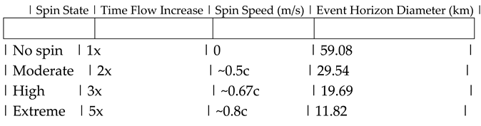
Worked Example (2x Time Flow Increase)

  • Mass = 10 × 1.989 × 10^30 = 1.989 × 10^31 kg
  • Diameter = 1.989 × 10^31 × 2.97033058787623 × 10^-27 = ~59,079.88 m
  • Altered Time Flow = (59,079.88 × 3.33564095 × 10^-9) + 1 = ~1.000197 s
  • New Time Flow = 2 × 1.000197 = ~2.000394 s
  • Spin Speed = 299,792,458 – ((1.000197 × 299,792,458) ÷ 2.000394) = ~149,896,234 m/s
  • New Horizon = ((59,079.88 × 3.33564095 × 10^-9) × (1.000197 ÷ 2.000394)) ÷ 3.33564095 × 10^-9 = ~29,539.94 m (~29.54 km)
  • Alternatively, New Horizon = 59,079.88 × ((299,792,458 – 149,896,234) ÷ 299,792,458) ≈ 29,539.94 m

Conclusion

Spin in the Temporal Dynamics framework does not modify gravity directly, but instead reshapes how time flows in space. This results in:
  • An inward shift of the event horizon,
  • A natural avoidance of singularities,
  • More complex gravitational behavior,
  • Potential mass-energy conversion through spin.
These insights align with observations of spinning black holes while offering a new theoretical lens for understanding their structure.

Temporal Dimensions and Variations in Time Flow

In the traditional framework of space-time, we often describe our universe in terms of three spatial dimensions and one temporal dimension. However, the concept of temporal dimensions suggests that time can flow at different rates in various contexts, leading to distinct temporal experiences or dimensions. Here’s an exploration of this idea:
  • Understanding Temporal Dimensions:
    -
    Temporal dimensions can be thought of as distinct realms where time flows differently, each characterized by its own specific rate of temporal progression. While we perceive time as a single linear flow, there exists the possibility of multiple temporal dimensions where time behaves in unique ways.
  • Universal Constants and Time Flow:
    -
    The universal speed of light (denoted as c = 299,792,458 meters per second) serves as a fundamental constant in our understanding of the universe. By expressing time flow in terms of universal constants, we can formulate a relationship: uc = {1}÷{299,792,458}. This relationship implies that different temporal dimensions can be defined by distinct values of universal constants. Each unique constant influences how time flows, creating a varied temporal dynamic that sets these dimensions apart from one another.
  • Separation of Temporal Dimensions:
    -
    Each temporal dimension operates independently, with its own fabric of time that does not necessarily interact with or relate to other temporal dimensions. For instance, if one temporal dimension has a flow where one second equals two seconds in our perception, then entities existing in this dimension would experience time distinctly, leading to unique physical and causal relationships.
  • Existence of Other Temporal Realms:
    -
    Just as there are multiple spatial dimensions—potentially more than the three we observe—there could be temporal dimensions that coexist alongside our own. These dimensions are just as real as our conventional perception of time, but they exist in isolation from our experiential framework, governed by their own rules and constants.
  • Implications for Physics and Cosmology:
    -
    The notion of multiple temporal dimensions raises intriguing questions about the nature of reality, causality, and the structure of the universe. It challenges our foundational understanding of physics and could offer insights into phenomena that seem paradoxical or unexplained within the confines of our four-dimensional space-time model.

Conclusions & Future Work

This research introduces the Temporal Dynamics Framework, proposing that gravity arises not from the curvature of space-time but from variations in the flow of time. Unlike General Relativity, which describes gravity as the distortion of space-time due to mass, this model treats space as structurally fixed, with time flowing at a fundamental rate. The presence of mass alters this temporal flow, creating gravitational effects as objects move through regions of varying time flow.
The framework successfuly derives gravitational acceleration using time-flow equations and predicts values for Earth and Mars that match empirical observations. It also provides an alternative explanation for motion, relativity, and black hole event horizons, suggesting that black holes do not collapse into singularities but accumulate mass at their event horizon, where time flow effectively halts.
Additionally, the research proposes that temporal dimensions may exist, influencing the nature of gravity and space-time interactions. This idea challenges conventional physics and opens new directions for theoretical and experimental investigations.
Key Takeaways
  • Gravity results from time flow variations, not space-time curvature.
  • Mass slows time flow, creating gravitational acceleration.
  • Objects of different masses fall at the same rate because they experience the same local time-flow gradient.
  • Black holes do not collapse into singularities but grow outward as mass accumulates at the event horizon.
  • Temporal dimensions could redefine our understanding of space-time interactions.
Future Research Directions
  • Experimental Validation: Future work should explore precise time-flow measurements around massive bodies, testing whether gravitational acceleration can be directly correlated to time-flow variations rather than space-time curvature.
  • Astronomical Observations: Studying black hole event horizons with high-resolution imaging could provide evidence for the accumulation model over singularity formation.
  • Implications for Cosmic Expansion: Investigating whether time flow variations influence cosmic expansion could refine our understanding of dark energy.
  • Mathematical Extensions: Further derivations are needed to unify this framework with existing relativistic and quantum theories, particularly regarding time-flow variations at microscopic scales.
By shifting the focus from space curvature to time-flow dynamics, this model offers a fresh perspective on gravitational interactions and the fundamental structure of reality. Future experimental and theoretical efforts will determine whether Temporal Dynamics provides a viable alternative to existing gravitational models.

Conflicts of Interest

The authors declare no conflicts of interest.

AI Disclosure Statement

In accordance with the Taylor & Francis AI Policy, I confirm that Generative Artificial Intelligence (AI) tools were used in the preparation of this manuscript. Specifically, ChatGPT (version 4.0) was utilized for:
  • Drafting and Refinement – Assisting in structuring the manuscript, enhancing clarity, and improving coherence in explanations related to temporal dynamics, space-time, and gravity.
  • Mathematical Formatting – Converting equations into linear text for readability and consistency with formatting guidelines.
  • Reference Compilation – Generating APA-style citations based on key sources in gravitational physics, space-time theory, and black hole dynamics.
  • Abstract and Summary Generation – Assisting in the development of an engaging abstract and structured conclusions.
The AI tool was not used for data analysis, hypothesis generation, or original scientific insights, and all final content was reviewed, edited, and approved by the author(s) to ensure academic integrity and compliance with publication standards.

References

  1. Einstein, A. The foundation of the general theory of relativity. Annalen der Physik 1916, 49(7), 769–822. [Google Scholar] [CrossRef]
  2. Newton, I. Philosophiæ Naturalis Principia Mathematica [Mathematical principles of natural philosophy]; Royal Society, 1687. [Google Scholar]
  3. Hawking, S. W. Particle creation by black holes. Communications in Mathematical Physics 1975, 43(3), 199–220. [Google Scholar] [CrossRef]
  4. Bekenstein, J. D. Black holes and entropy. Physical Review D 1973, 7(8), 2333–2346. [Google Scholar] [CrossRef]
  5. Schwarzschild, K. On the gravitational field of a mass point according to Einstein’s theory. Sitzungsberichte der Königlich Preußischen Akademie der Wissenschaften 1916, 189–196. [Google Scholar]
  6. Wald, R. M. General relativity; University of Chicago Press, 1984. [Google Scholar]
  7. Thorne, K.S. Black holes and Time Warps: Einstein’s Outrageous Legacy; W. W. Norton & Company, 1994. [Google Scholar]
  8. Carroll, S.M. Spacetime and Geometry: An Introduction to General Relativity; Addison-Wesley, 2004. [Google Scholar]
  9. Francis, O.O. Essence dynamics: Essence interactions, applications and Reality. Part I. Preprints 2024, 2024082057. [Google Scholar] [CrossRef]
Disclaimer/Publisher’s Note: The statements, opinions and data contained in all publications are solely those of the individual author(s) and contributor(s) and not of MDPI and/or the editor(s). MDPI and/or the editor(s) disclaim responsibility for any injury to people or property resulting from any ideas, methods, instructions or products referred to in the content.
Copyright: This open access article is published under a Creative Commons CC BY 4.0 license, which permit the free download, distribution, and reuse, provided that the author and preprint are cited in any reuse.
Prerpints.org logo

Preprints.org is a free preprint server supported by MDPI in Basel, Switzerland.

Subscribe

Disclaimer

Terms of Use

Privacy Policy

Privacy Settings

© 2025 MDPI (Basel, Switzerland) unless otherwise stated