
Submitted:
10 June 2025
Posted:
16 June 2025
You are already at the latest version
Abstract
The quest for a unified understanding of the cosmos necessitates novel theoretical frameworks that can reconcile General Relativity and Quantum Mechanics while explaining phenomena like dark matter and dark energy. This preprint introduces an Entropic Spacetime Framework rooted in a generalized action principle. It posits the existence of fundamental entropic scalar fields—a temporal field ($\ST$) and a spatial field ($\SSp$)—and a specific resonant coupling mechanism. We outline the framework's mathematical foundations and present compelling initial evidence for its validity: a numerical simulation that successfully reproduces the observed Milky Way rotation curve without requiring dark matter. Furthermore, we demonstrate how the framework offers an intuitive, mechanical explanation for Hawking radiation. We invite critical feedback and collaboration from the theoretical physics community to refine and further develop this promising new direction.
Keywords:
entropic spacetime
; emergent gravity
; emergent spacetime
; generalize action principle
; scalar field cosmology
; resonant compling
; entropic fields
; foundations of physics
; quantum gravity
; cosmology
; astrophysics
; general relativity
; modified gravity
; hawking radiation
1. Introduction: The Unfinished Picture of Physics
The universe, as we understand it, is governed by two supremely successful yet fundamentally incompatible theories: General Relativity (GR), which describes gravity and the large-scale structure of the cosmos [1], and Quantum Mechanics (QM), which governs the microscopic world. This foundational schism, coupled with the mysteries of dark matter, dark energy, and the fine-tuning of fundamental constants, signals that our current understanding is incomplete.
This proposal offers a fresh perspective: an Entropic Spacetime Framework that seeks to unify physics by tapping into the very essence of entropy and resonance. This paper introduces the core conceptual and mathematical foundations of this framework and discusses how this approach naturally addresses key cosmological challenges. Crucially, we then move beyond pure theory to present initial validation: a detailed phenomenological application to the persistent enigma of galaxy rotation curves, which demonstrates the framework’s ability to explain observed phenomena without recourse to conventional dark matter assumptions.
2. The Entropic Spacetime Framework
2.1. Foundations: From 4D Continuum to Emergent Spacetime
Traditional GR describes spacetime as a unified four-dimensional manifold. This framework proposes a reconceptualization, viewing spacetime as dynamically emerging from distinct 3D spatial and 1D temporal components, a perspective supported by formalisms such as ADM [2] and conceptual models from fluid dynamics [3] and quantum information theory [4,5]. Building on these insights, our work proposes a concrete field-based realization, with a spatial entropic field serving as an entanglement-bearing medium and a temporal entropic field providing a dynamical, local realization of time’s arrow, inspired by de Broglie’s "internal clock" [6,7].
2.2. The Generalized Action Principle
The mathematical bedrock of this framework is a generalized action principle. The total action, S, extends the conventional Einstein-Hilbert action () [1,8] by incorporating terms for the entropic fields and their interactions:
Here, describes the intrinsic dynamics of the entropic fields, while dictates their specific interactions with the spacetime metric () and standard matter fields, interpreted as a "resonant" mechanism.
2.3. The Nature and Dynamics of Entropic Fields ()
The framework hypothesizes two primary scalar fields: a temporal entropic field, , and a spatial entropic field, . Their dynamics are governed by a Lagrangian containing standard kinetic terms and a potential term, . The equations of motion are derived from the variational principle [9]:
Here, and are source terms arising from the coupling action. The temporal field is hypothesized to inherently possess a directedness, providing a physical basis for the arrow of time, analogous to concepts in Entropic Dynamics [10].
2.4. The Resonant Coupling Term (Scoupling)
A crucial interpretive directive is to consider as a "resonant term." This implies that the interactions are not uniform but are selective and context-dependent, becoming pronounced only when the frequency or energy scale of a system matches inherent frequencies of the entropic fields. This provides a natural filter that could explain why cosmic-scale phenomena might be influenced by these fields while everyday laboratory scales are not.
3. Illustrative Applications and Results
3.1. Galactic Dynamics: A Numerical Solution to the Rotation Curve Problem
The galaxy rotation problem presents a crucial test for the framework. The simulation solves the coupled field equations for the Milky Way on a 2D grid, with the core PDE taking the form:
The model was trained by minimizing a chi-squared loss function between the total predicted velocity () and observed velocity data. The 2D simulation successfully reproduced the observed flattening of the Milky Way’s rotation curve, as shown in Figure 1.
The simulation learned a significant, non-zero entropic field configuration that, when translated to a velocity component, provides the exact amount of additional support needed to counteract the natural Keplerian decline. tab:learnedparams shows the final learned values of the model parameters.
3.2. Black Hole Thermodynamics: A Qualitative Model for Hawking Radiation
Beyond galactic dynamics, the framework offers an intuitive, mechanical explanation for Hawking radiation. If spacetime itself is a quantized, fluctuating field, the region near an event horizon is not a smooth manifold but a region of energetic "boiling" of the spacetime fabric. In this view, Hawking radiation is the direct emission of real particles from these fluctuations. The intense gravity warps the field, exciting its high-frequency modes. Occasionally, a fluctuation becomes so energetic that it decouples and propagates away as a real particle, carrying energy from the black hole. This mechanism naturally incorporates the inverse relationship between black hole mass and temperature. The detailed mathematical underpinnings are outlined in Appendix C.
4. Discussion
4.1. Current Limitations and Future Directions
The framework, while promising, faces significant limitations. The precise mathematical forms of the potential and the coupling term are currently undefined. There is no direct experimental evidence for the entropic fields. Future work must focus on developing specific, physically motivated mathematical forms for the potential and coupling terms, and extending the simulations to other galaxies and phenomena like gravitational lensing. Identifying unique experimental signatures is paramount.
4.2. Speculative Aspects
The extensions of this framework to explain the origin of life and consciousness are highly speculative. The framework’s core tenets suggest compelling implications for quantum computation, potentially reframing our understanding of the Heisenberg Uncertainty Principle as an intrinsic property of the spatial medium and suggesting that advanced quantum computers might learn to harness and sculpt entropic flows.
5. Conclusion
The Entropic Spacetime Framework offers a conceptually rich and ambitious vision for unifying diverse phenomena. Its strength lies in introducing interpretable degrees of freedom and a flexible, resonant interaction mechanism. Its intuitive appeal and the successful initial validation against the Milky Way rotation curve make it a compelling avenue for future foundational research. However, the framework is currently a meta-theoretical proposal, requiring significant work in detailed model building and phenomenological testing to become a fully predictive scientific theory.
Acknowledgements
We acknowledge Boston Children’s Hospital and Harvard Medical School for their support. Special thanks to A.I. Assistant Gemini (Google) and ChatGPT for their invaluable assistance in the early formulation and refinement of this framework.
Appendix A. Detailed Derivation of Field Equations
This appendix provides a more detailed mathematical exposition of the field equations introduced conceptually in the main text. It outlines specific forms for the entropic and coupling actions and demonstrates how the modified gravitational and entropic field equations are derived from the generalized action principle.
Appendix A.1. Defining the Entropic Action (S entropic )
This section focuses on the intrinsic dynamics of the temporal entropic field () and the spatial entropic field (). Assuming they are scalar fields, the entropic action is given by the integral of the Lagrangian density () over spacetime, multiplied by the square root of the determinant of the metric tensor:
The Lagrangian density, , is stated to naturally include kinetic terms for each field and a potential term that governs their self-interactions and mutual interactions.
Appendix A.1.1. Kinetic Terms for ST and SS
The standard canonical kinetic terms for real scalar fields are proposed as appropriate initial candidates:
Considerations for directedness might arise from the potential or coupling, but a simpler approach is to encode this directedness there.
Appendix A.1.2. The Potential Term V(ST, SS)
This is identified as the most crucial part of as it dictates the self-interactions of the entropic fields, their masses, and their vacuum states. The specific mathematical form of this potential will determine the field configurations corresponding to minima, their effective masses, and their capacity to drive cosmological dynamics. Inspiration for its form can be drawn from potentials used in inflationary models, quintessence/dark energy models, and Higgs-like potentials. A conceptual equation by Gowan is also mentioned, suggesting a relationship between spatial and temporal entropy that might be reflected in through interaction terms. An example form for a general polynomial potential is provided:
The specific coefficients of this potential would be constrained by phenomenological requirements.
Appendix A.2. Defining the Coupling Action (Scoupling )
This term describes how and interact with the spacetime metric and with standard matter/radiation fields. It is interpreted as a resonant term, implying that interactions are selective and frequency-dependent.
Appendix A.2.1. Identifying Interacting Components
The interacting components include the metric () the entropic fields (,) and their derivatives, and matter fields (fermions, gauge bosons, other scalars).
Appendix A.2.2. Direct Coupling to Matter Fields
Yukawa-type (scalar-fermion):
Scalar-gauge boson (Electromagnetic Coupling): (axion-like coupling). These terms explicitly describe how the entropic fields (,) interact with the electromagnetic field () and thus with light and other forms of electromagnetic radiation, potentially affecting its propagation, polarization, or other properties. Similar terms would exist for .
Derivative couplings: where is a matter current. These couplings will define the and terms in Equations (2) and (3) of the main text.
Appendix A.2.3. Incorporating "Resonance" into Scoupling
This is achieved by making coupling parameters functions of entropic fields or other relevant quantities (e.g., ), or by introducing new intermediate fields. An effective field theory approach suggests that interaction terms might become significant only under specific conditions (e.g.. temperature, density, or characteristic frequencies of the matter sector). Developing a rigorous, possibly non-local, formulation of this frequency-dependent coupling is part of our ongoing work.
Appendix A.2.4. Role of Fast Fourier Transform (FFT)
FFT can be used as an informative tool to analyze characteristic frequencies of phenomena (e.g., biological rhythms, neural oscillations). These identified frequencies can then guide the construction of to maximize coupling when a dynamical aspect of or aligns with the system’s characteristic frequencies.
Appendix A.2.5. Drawing Inspiration from Einstein-Cartan (EC) Theory
EC theory (extending GR by allowing torsion coupled to spin density)[? ?] offers conceptual parallels, suggesting how new geometric degrees of freedom can interact with intrinsic properties of matter beyond standard energy-momentum.
Appendix A.3. Derivation and Analysis of Field Equations
Once specific forms for and are postulated, the field equations can be derived using the variational principle.
Appendix A.3.1. Deriving
This is the stress-energy tensor for the entropic fields. For canonical scalar fields (where ) with potential , it can be expressed as:
Then, (interaction terms from )
Appendix A.3.2. Deriving
This term represents modifications to the geometric side of Einstein’s equations. It arises from terms in or that explicitly involve curvature or couple directly to the metric. For example, if , then varying this plus with respect to yields terms contributing to
Appendix A.3.3. Deriving CT and CS
These are the coupling terms in the entropic field equations (Equations (2) and (3) in the main text). They are derived from the variation of with respect to and . For example, if , then .
Appendix A.3.4. Illustrative Field Equations
Assuming simplified forms for the entropic and coupling Lagrangians, the modified gravitational and entropic field equations can be illustrated:
The modified gravitational equations would conceptually be:
The exact terms for and require careful derivation based on the precise definition of and how its variation with respect to is allocated.
Appendix A.3.5. Detailed Illustrative Derivations
Below is a concrete, step-by-step illustration of how one would go from the illustrative actions in your manuscript to the field equations and metric variation terms. This derivation is kept general so you can later slot in whatever specific potential or "resonant" coupling functions you choose but explicit enough that you can see every piece of the variational calculus.
Appendix A.3.3.1. Entropic Action S entropic :
We start from the entropic action:
1.1 Equations of motion for ST and SS:
For a generic scalar field with Lagrangian density the Euler-Lagrange equation in curved space is:
Kinetic term variation: , so (the covariant d’Alembertian). Potential term variation: and . Putting it together: equation: equation: Or compactly:
1.2 Variation with respect to gμν ⟶ :
Recall Key identities: , The kinetic part varies to:
and the potential part to: Putting it all together:
Coupling Action Scoupling:
The illustrative form is:
with the understanding that in the full "resonant" version and become functions of .
2.1 Variation with respect to the metric gμν:
To see how these couplings modify Einstein’s equations, compute . Standard variations needed: Metric determinant: Ricci scalar: Matter Lagrangian: , defining the usual stress-energy . Putting these in gives the effective stress-energy from :
Here each term comes from one of the variations above. In the "resonant" version, will be replaced by its more elaborate field-dependent form.
2.2 Nonminimal coupling :
Focus on Vary , holding fixed. Use: Multiplying by yields two pieces: and . Thus the modification on the LHS of Einstein’s equations is:
2.3 Direct matter coupling :
Consider . Varying (with fixed, but depending on g) gives two contributions: and One finds: Hence the extra stress from matter coupling is
Putting everything into the Modified Einstein Equations:
The total action is: Varying with respect to . You obtain the modified Einstein equations
Where: from Appendix B.2 (the non-minimal pieces) from Appendix B.1.2 from Appendix B.3 And the scalars obey: once you include their coupling-induced source terms (just vary the total action w.r.t. ).
Appendix A.4. Examples of Coupling Term Functional Forms
This section outlines various functional forms for the coupling terms and which can be used to implement specific "resonance" or context-dependent behaviors for the entropic couplings.
Appendix A.4.1. Gaussian “band-pass” in field space
Peaks the coupling when lie near some preferred values (,):
and similarly Resonance occurs when the fields approach the “center” (,). The widths control how sharply peaked the resonance is.
Appendix A.4.2. Lorentzian (Breit–Wigner) Profile
Gives long tails for “near-miss” resonances:
(and analogously for ). Here set the half-width at half-maximum.
Appendix A.4.3. Logistic (Step-Like) Gating
Ideal if you want almost zero coupling below a threshold and nearly constant above:
large ⇒ sharp switch-on at the “resonant” field values. Can be used alone or multiplied by one of the peaked forms above for combined gating and tuning.
Appendix A.4.4. Frequency-domain resonance
If in your simulation you can track the local time-series , you can Fourier-analyze it and let the coupling depend on the spectral amplitude at some frequency . E.g.
where is the frequency at which is maximal in your local patch. This realizes a truly dynamical resonance in time.
Appendix A.4.5. Combined forms
Appendix A.4.6. How to Choose Parameters
- Centers : pick based on where/when you want coupling to peak in your simulation.
- Widths : tune so the resonance is broad enough to capture the phenomenon but narrow enough to remain “selective.”
- Amplitudes : set by the overall strength of the entropic effects you want to explore.
These functional forms comprise a flexible toolkit for building in the “resonant,” context-dependent behavior of entropic couplings.
Appendix A.4.7. Next Steps
- Choose a specific potential and explicit functional forms , to implement your “resonance.”
- Plug those into the above general formulas.
- Use symbolic algebra software (e.g. xAct in Mathematica) to handle the tensor algebra and covariant derivatives.
Appendix B. Variational Analysis
This appendix provides a fully detailed walk-through of every variational step needed to go from your ansatz actions to the field equations and stress–energy tensors. It is broken into three parts:
- Varying to get the scalar EoMs and
- Varying the non-minimal curvature couplings to extract their contribution on the LHS of Einstein’s equations.
- Varying the direct matter couplings to get the additional stress tensor .
Appendix B.1. Sentropic → Scalar EoMs and Entropic Stress Tensor
We start with
Appendix B.1.1. Variation w.r.t. ST (same for SS)
Compute . . Integrate by parts the kinetic term:
Here we used:
and dropped total derivatives. Euler–Lagrange equation: Or compactly .
Appendix B.1.2. Variation w.r.t. gμν →
Recall We need variations of Key identities: Kinetic piece: Carefully collecting signs yields the standard scalar–field stress tensor. Potential piece: Putting it all together,
Appendix B.2. Non-Minimal Coupling ∫
Focus on We vary w.r.t. , holding fixed. Use the well-known identity Multiplying by , we get two pieces: Einstein–tensor shift Derivative terms These together define the modification on the LHS of Einstein’s equations:
Appendix B.3. Direct Matter Coupling
Consider Again vary , treating fixed but allowing to depend on g. One finds:
Two sources of variation
Result Hence the extra stress from matter coupling is
Appendix B.4. Putting it all together
Vary the full action w.r.t. . You obtain the modified Einstein equations Where: from Appendix B.2 (the non-minimal pieces) from Appendix B.1.2 from Appendix B.3 And the scalars satisfy once you include their coupling-induced source terms (just vary the total action w.r.t. ).
Appendix B.5. Next steps
- Choose a specific potential and explicit functional forms , to implement your “resonance.”
- Plug those into the above general formulas.
- Use symbolic algebra software (e.g. xAct in Mathematica) to handle the tensor algebra and covariant derivatives.
content for Appendix B goes here, detailing the variational calculus.)
Appendix C. Quantization and Advanced Applications
Appendix C.1. Application to Black Hole Thermodynamics and Hawking Radiation
The conceptual model of Hawking radiation described in Section 3.2 can be formalized. We consider the dynamics of the entropic fields in a fixed Schwarzschild background metric. The core of the new physics comes from how we model the "boiling" of spacetime. We propose that the quantum fluctuations of the field become amplified by the gravitational potential. A simplified, effective model for a fluctuation field near the horizon can be described by a stochastic differential equation:
where is a stochastic noise term whose amplitude is amplified by the local gravitational field strength, posited as . Particle emission occurs when a fluctuation’s energy exceeds a critical threshold. The rate of emission, , is proportional to the probability of this occurrence:
This last step connects to the standard Bekenstein-Hawking temperature result, , providing a qualitative path to deriving black hole thermodynamics from the framework.
Appendix D. The Human-AI Collaboration: A New Paradigm for Theoretical Physics
This Entropic Spacetime Framework was developed over approximately two months through a close collaboration between human intuition and advanced Artificial Intelligence. This appendix details the nature and dynamics of this human-AI partnership.
Appendix D.1. Roles and Interplay in the Development Process
The collaboration evolved through distinct roles. The human contributor served as the initiator and intuitive guide, defining the core problem, providing high-level validation, and setting the strategic research path. The AI (Gemini and ChatGPT) acted as a knowledge synthesizer and ideation partner, performing rapid literature reviews, identifying relevant mathematical formalisms, suggesting standard Lagrangian forms, and assisting in drafting and refining the manuscript.
Appendix D.2. Implications for Future Scientific Discovery
This project exemplifies a burgeoning new paradigm for theoretical science: a symbiotic partnership where human creativity and strategic direction are amplified by AI’s capacity for information synthesis and rapid ideation. It suggests that future breakthroughs may increasingly arise from such augmented intelligence, accelerating the pace at which grand challenges can be tackled.
References
- Albert Einstein. “Hamiltonsches Prinzip und die allgemeine Relativitätstheorie”. In: Sitzungsberichte der Königlich Preußischen Akademie der Wissenschaften (Berlin) (1916), pp. 1111– 1116.
- Richard Arnowitt, Stanley Deser, and Charles W. Misner. “The Dynamics of General Relativity”. In: Gravitation: An Introduction to Current Research. Ed. by Louis Witten. New York: Wiley, 1962, pp. 227–265.
- T. Padmanabhan. “Gravity and the thermodynamics of horizons: A perspective on spacetime microstructure”. In: Physics Reports 406.2 (2005), pp. 49–125. [CrossRef]
- Mark Van Raamsdonk. “Building up spacetime with quantum entanglement”. In: General Relativity and Gravitation 42.10 (2010), pp. 2323–2329. [CrossRef]
- Brian Swingle. “Spacetime from entanglement”. In: Annual Review of Condensed Matter Physics 9 (2018), pp. 345–358.
- Louis de Broglie. “Recherches sur la théorie des quanta”. In: Annales de Physique 10 (1925), pp. 22–128.
- M. Basil Altaie, D. Hodgson, and A. Beige. “Time and Quantum Clocks: A Review of Recent Developments”. In: Frontiers in Physics 10 (2022), p. 897305. [CrossRef]
- David Hilbert. “Die Grundlagen der Physik (Erste Mitteilung)”. In: Nachrichten von der Gesellschaft der Wissenschaften zu Göttingen, Mathematisch-Physikalische Klasse (1915), pp. 395–408.
- David Hilbert. “Mathematische Probleme”. In: Nachrichten von der Kgl. Gesellschaft der Wissenschaften zu Göttingen, Mathematisch-physikalische Klasse (1916), pp. 253–297.
- Ariel Caticha. “Entropic dynamics”. In: Entropy 17.9 (2015), pp. 6110–6128.
Figure 1.
Final fit of the Entropic Spacetime model to the Milky Way rotation curve. The total model (red line) shows a strong agreement with the observed data (black dashed line).
Figure 1.
Final fit of the Entropic Spacetime model to the Milky Way rotation curve. The total model (red line) shows a strong agreement with the observed data (black dashed line).
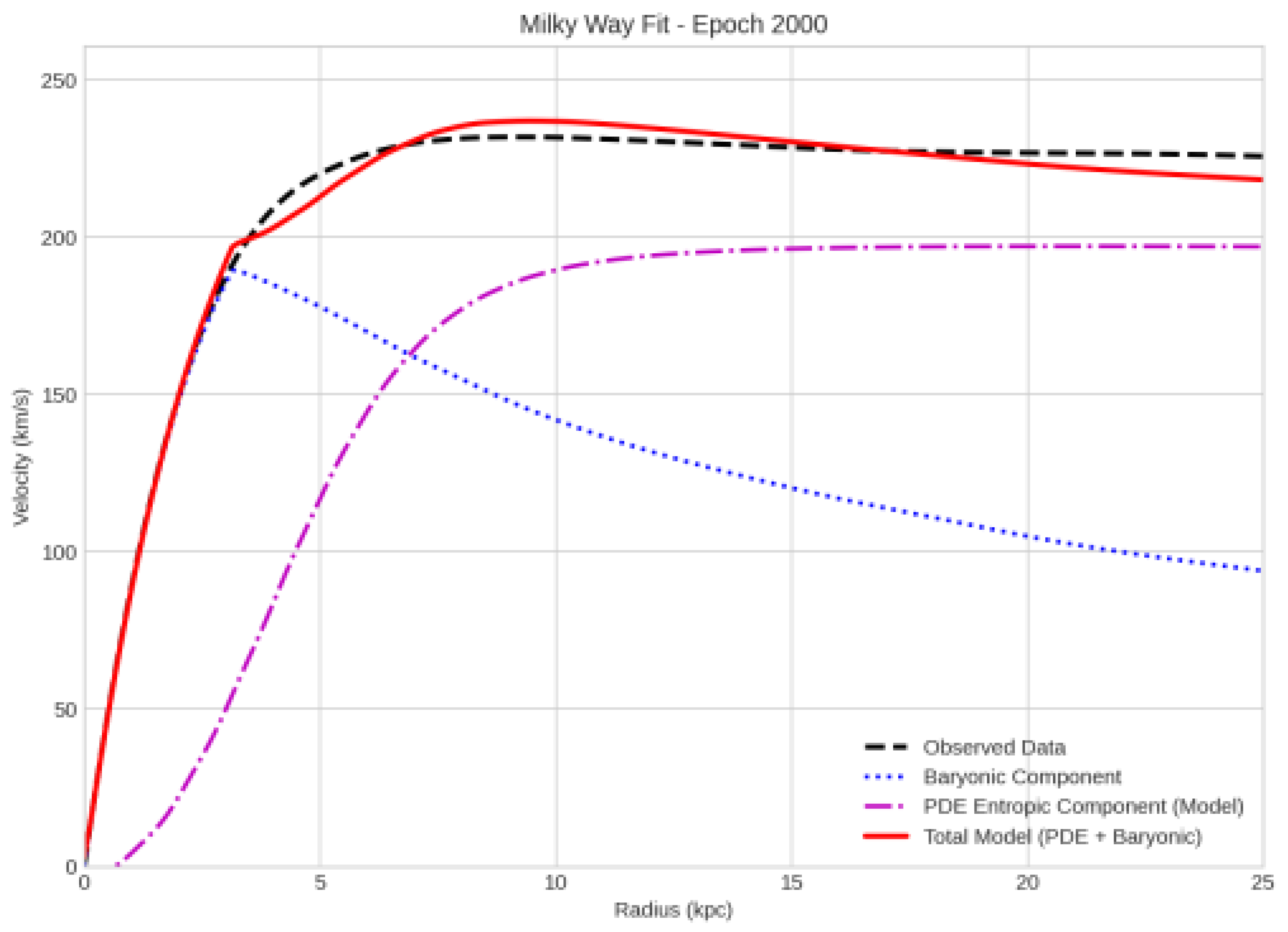

Table 1.
Final Learned Parameters from the Milky Way Simulation.
| Parameter Name | Final (Learned) Value |
|---|---|
| PDE Dynamics | |
| Diffusion () | 0.200789 |
| Self-Interaction () | -0.015241 |
| Self-Interaction () | -0.010046 |
| Constant Source () | 0.000015 |
| Coupling Terms | |
| Resonant Coupling Amp. () | 0.009386 |
| Resonance Center () | 0.100030 |
| Gravitational Coupling () | 0.011833 |
| Velocity Mapping | |
| Velocity Scale () | 197.618497 |
| Velocity Offset () | -0.000018 |
Disclaimer/Publisher’s Note: The statements, opinions and data contained in all publications are solely those of the individual author(s) and contributor(s) and not of MDPI and/or the editor(s). MDPI and/or the editor(s) disclaim responsibility for any injury to people or property resulting from any ideas, methods, instructions or products referred to in the content. |
© 2025 by the authors. Licensee MDPI, Basel, Switzerland. This article is an open access article distributed under the terms and conditions of the Creative Commons Attribution (CC BY) license (http://creativecommons.org/licenses/by/4.0/).
Copyright: This open access article is published under a Creative Commons CC BY 4.0 license, which permit the free download, distribution, and reuse, provided that the author and preprint are cited in any reuse.


