
Submitted:
11 March 2025
Posted:
13 March 2025
You are already at the latest version
Abstract
Spatial gridshells are characterized by large spans, expansive interior spaces, structural efficiency, and aesthetic appeal. Among these, elastic gridshells are particularly noteworthy as they utilize the elastic deformation of components to create freeform surfaces. However, current approaches to modular design of elastic gridshells predominantly rely on optimization methods, which are often tricky to find initial geometry, inefficient, and impractical for real-world design scenarios. This work introduces an algorithmic design method based on the Conformal Principal-Asymptotic (CPA) network on minimal surfaces (MS), enabling efficient parametric design and modular construction of elastic gridshells. The algorithm provides a versatile design space, of various shapes for the shells design, and various configurations and sections for the beams design. As well as, precise (geometry-based) assembly-stress analysis and quantitative performance evaluation for architectural applications. Finally, an example of the algorithm's application to a real construction project is provided, demonstrating its effectiveness and ease of use for designers.
Keywords:
elastic gridshell
; architectural geometry
; parametric design algorithm
; minimal surfaces
; principal/asymptotic networks
; modular construction
1. Introduction
Gridshells, a type of spatial structure, are widely used in the design of large-span buildings. Gridshells can be primarily classified in two ways: the first classification is based on whether the beams are continuous, resulting in either discontinuous gridshells (such as the British Museum roof) or continuous gridshells (such as the Mannheim Multihalle). The second classification depends on whether the assembly of beams requires pre-existing elastic deformation, distinguishing between rigid gridshells (like the Schuber Club Band Shell) and elastic gridshells (like the Mannheim Multihalle). It is known that, elastic gridshells (freeform surface structures assembled from networks of beams undergoing elastic deformation) are efficient structural solutions, as they cover large spans with minimal material usage. A clear challenge to them, is the complexity of construction of these doubly-curved surfaces. In response to this challenge, the field of architectural geometry [27] emerged with the goal of developing sustainable fabrication methods for these complex designs. Current research in this field, that is relevant to this work involves: modular surface panels, modular joints and modular beams.
1.1. Elastic gridshells from CPA networks
This work focuses on the design of elastic gridshells generated from CPA networks on MS. The process of creating a elastic gridshell begins with generating a network of curves on a geometrically defined surface. These curves will then give rise to surface strips (from specific vectorfields along the curves). By giving these strips a certain thickness, they are transformed into laths, which then compose the final elastic gridshell structure. To better design elastic gridshells, the focus is placed on networks formed on precisely defined geometric surfaces. As illustrated in Figure 1, the principal network offers several construction advantages: all joint connectors right-angled; all panels are planar without acute angles; strips generated from principal curves are developable (i.e. can be unrolled without deformation); and finally, planar laths can be positioned under pure bending. The asymptotic network also has its construction benefits: normal strips along network curves can be unrolled into nearly straight bands, and straight planar laths can be positioned under bending and twisting. From another side, MS are known to be isothermic (i.e. admiting conformal principal (CP) parameterizations), these can be generated from the (conformal) spherical image of the MS, by integrating the Christoffel-dual system, refer to [6]. In fact, this system comes with an adjoint differential system (from the same spherical image), refer to [11]. Integrating it, yields an adjoint conformal asymptotic (CA) MS-patch, thus a CPA pair of adjoint MS-patches, giving rise to “CPA elastic gridshell”. Moreover, the principal and asymptotic networks (on each of the adjoint MS CPA pair) can be generated such that they match each other’s intersection points, creating a rich design space.
Note that, existing design methods for CPA elastic gridshells primarily rely on optimization techniques [32] or the sequential tracing of asymptotic and principal curves on predefined MS [30]. The optimization approach begins with a random initial shape and defines a discrete version of asymptotic and principal networks, as its optimization objective. Even though the result meets the design requirements, this method faces challenges in defining the initial geometry, making it difficult to achieve optimal results. In contrast, the tracing method starts with a classical MS as a fixed design shape and iteratively solves for the network distribution by selecting any point on the surface and tracing the asymptotic and principal curves step by step (which can be time-consuming). While this method ensures accurate network generation on MS, it suffers from being less time-efficient, and having a limited design space, as it does not address the creation of diverse MS. The mentioned limitations of both methods, make them slightly less suitable for effective architectural design applications. A parameterized definition of CPA MS-patches is believed to better fulfill practical design requirements; however, research in this area remains limited, making this work a step toward addressing this gap.
1.2. Contributions and Overview
This article aims to introduce a practical parametric design algorithm specifically developed for the rapid design, optimization, and modular construction of CPA elastic gridshells. The main contributions are:
-
An algorithm for parametric design, analysis, modular construction of CPA elastic gridshellsIn Section 2, we provide a detailed method for generating CPA MS-patches for parametric design (Section 2.1). We demonstrate that these MS-patches exhibit rotation / reflection symmetries and, in some cases, periodicity, which contribute to modularity in construction (Section 2.2). Furthermore, we introduce methods for varying the shapes, thereby expanding the design space (Section 2.3). Next, we generate strips from curves on the surface and analyze their geometric properties (Section 2.4), which are essential for subsequent analysis of active-bending / twisting beams stresses (Section 3.2.2).
-
A parameterized space for morphological analysis of shape and configuration variantsIn Section 3, we establish a parameterized space of MS-patch variations (Section 3.1), all of which adhere to geometric properties that favor fabrication. Section 3.1.1 to Section 3.1.3 focus on shape variants, presenting different methods for transforming shape parameters. Section 3.1.4 addresses configuration variants, exploring how various configuration types can be generated. This is done by selecting different strip types and combinations. As well as redistributing configurations through patch reparameterization. This approach provides designers with an efficient and precise method for conducting morphological studies within constraints optimized for fabrication. Additionally, we illustrate how these variants can be selected based on architectural and structural criteria (Section 3.2). The parametric nature of the space of variants greatly enhances the selection process, offering a concrete way to compare design options that share the same fabrication advantages. This allows for "local optimization" among neighboring variants, based on criteria such as spatiality (Section 3.2.1), active-bending / twisting beam stress, and stiffness of structure (Section 3.2.2). Regarding modular surface panels, using planar panels [10,12,28] and using spherical panels [7,16]. Next, for modular joints using conical meshes [17] (free offset nodes) and using principal symmetric meshes [23,24] (nodes with fixed angles). Finally, for modular beams, using principal curves [22], asymptotic curves [29,30], geodesic curves [21,25,26], pseudo-geodesic curves [19,36], planar curvature lines [20], as well as generating classic nets such as the Chebychev net [33,34].
-
Application and validation of the algorithm in a real construction project, incl. design workflowWe finally conclude the article, with a case study involving the realization of a full-scale pavilion (Section 4), providing a hands-on implementation of these geometrically pre-rationalized design methods and thereby demonstrating a proof-of-concept. Note that, in this process, we trace the entire trajectory from abstract mathematical theory to concrete material construction. This integrated multidisciplinary process ultimately offers valuable insights into the discrepancies between theory and practice and generates a workflow to guide the use of this parametric design algorithm by architects and engineers (Section 5).
2. Geometric Method from MS Theory
In this section, we will combine different mathematical concepts from MS theory, for more details refer to [9,11,14], into a geometric method to generate CPA MS-patches customized for parametric design application. In Section 2.1, we generate CPA MS-patches by solving a differential system, which we combine with holomorphic functions. In Section 2.2, we discuss properties of reprameterizations, symmetry and periodicity for CPA MS-patches. In Section 2.3, we show how to generate variations of CPA MS-patches to enrich the design choices, in particular using Bonnet and Goursat transforms. Finally, in Section 2.4, we study the geometry of strips derived along network curves of CPA MS-patches, presenting results applied in relating curvature and stresses (refer to Section 3.2.2). Note that for the sake of a smoother reading, mathematical proofs were pushed to the Appendix A.
2.1. Generation of CPA MS-Patches
To begin let us give the precise definitions of CPA MS-patches, to this end let us start be recalling the following notions. Let denote the standard Euclidean scalar product on and let denote its associated norm. In this paper, a surface is always given by a smooth parameterization patch with values in where in some open set in . The normal vector field to the surface defines a smooth parameterization with values in the unit sphere , called the spherical image of the surface. The partial derivatives allow us to define the coefficients of the first and second fundamental forms of X. Similarly, allow us to define the coefficient of the first fundamental form of N. The Gaussian and Mean curvatures are denoted by and respectively, in particular, if vanishes identically, then X is said to be MS-patch. Moreover, a patch X is Conformal Principal (CP), resp. Conformal Asymptotic (CA), if it satisfies:
A pair with a CP MS-patch and CA MS-patch having a common (necessarily conformal) spherical image will be referred to as CPA MS-patches, also known as adjoint pair.
2.1.1. Differential System and Holomorphic Functions
The subject of CPA MS-patches has been extensively studied by [11]. In particular, we have a result that states that to each conformal patch N with conformal factor (equals ), we have a unique pair of CPA MS-patches , which are obtained by respectively solving the systems:
Note that, the CP MS-patch X obtained by solving of differential system (2)(1) is in fact the Christoffel dual of the conformal patch N on the unit sphere, refer to [6]. For a discrete version of this Christofell duality construction generating discrete isothermic MS, refer to [3,4]. Therefore, a variation of the conformal patch N, yields a variations of CPA MS-patches. Now, in order to do such a variation of N, we will fix a known conformal patch on the unit sphere, defined by the inverse of the stereographic projection (from north pole) and denoted . Then, using the fact that regular holomorphic functions are conformal, we further compose with a holomorphic map defined on (a domain in) , resulting in a conformal patch N that varies as varies. More precisely, we have that:
Furthermore, the patch has more properties that will be useful later in showing the symmetries of the CPA MS-patches. In particular, it sends radial lines through the origin (in the plane) to geodesics (great circles) through the poles, that is, vertical meridians. In view of the above discussion we can thus state that:
Theorem 2.1.
Every holomorphic function Ψ gives rise to a pair of adjoint CPA MS-patches.
2.2. Properties of CPA MS-patches
We will now exhibit geometric properties of CPA MS-patches, having important fabrication implication.
2.2.1. Reparameterizations
There are two natural reparameterizations that arise from the CPA MS-patches as follows.
• Reparameterization-A: Consider the reparameterizations of the CPA MS-patches given by:
This reparameterization induces networks that are said to be corresponding, refer to [18]. This means, if we take a discrete number of -curves equally spaced in both directions (in parameter space), and a discrete number of -curves also equally spaced in both directions (in parameter space). It then follows that, the images of these networks through X and Y, are perfectly passing through each other’s intersection points, as seen in Figure 2. In particular, we have that:
Lemma 2.2.
The pair form CPA MS-patches, with is CA and is CP.
We have thus established a reparameterization yielding principal and asymptotic networks in correspondence, which has a fabrication advantage as seen in Figure 1.
• Reparameterization-B: We give another reparameterization of the CPA MS-patches , given by the Weierstrass function . For that we observe that give rise to a complex curve whose (complex) derivative satisfies . Therefore, the curve C admits the EW-representation as the integral (of ):
The complex variable is defined as and the functions are referred to as the Weierstrass data. The function is equal to the initial holomorphic function (associated to the CPA MS-patches) and the function can be determined by the ’s. The (complex) integral of the EW-representation (5) will be used in Section 2.2.2 to determine the periodicity of the CPA MS-patches , which is important for the modularity of the construction. Finally, let be the inverse of with (complex) derivative , then the Weierstrass function is given by inducing the reparameterizations:
for and .
2.2.2. Modularity
There are two natural properties of the CPA MS-patches that influence modularity of construction.
• Symmetry: The presence of symmetry axes, contributes to modularity of fabrication, which is a great advantage.
The idea is that, the surface can be constructed by reflection or rotation (of a part of it) about some symmetry axes. Let us now, describe the symmetry axes for CPA MS-patches. To begin, observe that a planar curve (whose plane is perpendicular to the MS) is a geodesic principal curve, that forms a reflection symmetry axis, while a straight line (in the MS) is a geodesic asymptotic curve, that forms a rotation (by 180°) symmetry axis. Next, in the particular setting of the CPA MS-patches with N their common spherical image, these symmetry axes are in fact network -curves. Thus, a planar u-curve in X (whose plane is perpendicular to the MS) is a reflection symmetry axis, corresponding to a straight u-curve in which is rotation symmetry, and both correspond to a great circle in N. That is we have:
Clearly, the above description is true for v-curves as well. The presence of symmetry axes allows us to define a Module-patch bounded by them, and “tilling” the MS (by reflections and rotations), as seen in Figure 3.
• Periodicity: The presence of periodicity, contributes to modularity of fabrication, as the surface can be constructed by repetition (of a part of it) along one, two or three directions, as seen in Figure 3. As mentioned earlier, knowing the EW-representation (5) of the CPA MS-patches enables us to determine the periodicity of the MS. The idea is to consider contour integrals along (simple) closed loops in the domain of the complex isotropic curve around singular points of the Weierstrass data . Making use of Cauchy’s residue theorem, the contour integral of C (holomorphic on ), defines the (complex) period vector , [37]:
This (complex) period functions characterize the periodicity of . Namely, X is called singly (resp. doubly or triply) periodic if X admits one (resp. two or three) non-zero period vector(s) . The same is said for where the period vector(s) is of the form . Note that the CPA MS-patches X and need not have the same periodicity. We have thus established the characterization of geometric modularity (by symmetry and periodicity) of the CPA MS-patches , necessary for our modular fabrication.
2.3. Variations of CPA MS-Patches
We will show how to generate variations in the CPA MS-patches in three different levels, while preserving their geometric properties. This will naturally enrich the shape design variety of the proposed parametric method, allowing the designer multiple design freedoms (Section 3.1).
2.3.1. Choice of Holomorphic Function
The first level of variations arises from the choice of the holomorphic function augmented with extra design parameters . For the sake of clarifying the method for the reader, we will present here six basic examples of CPA MS-patches induced by holomorphic functions, refer to Figure 4. Note that, there is an infinite number of choices of holomorphic functions that can be assigned. Let us now describe the modularity properties (i.e. symmetry and periodicity) of the six-types of CPA MS-patches.
Theorem 2.3.
Consider the CPA MS-patches of the six types in Figure 4, then:
- (1)
- All of them admit symmetry axes, in particular for:
- (2)
- Möbius, Cotan, Cubic-types are non-periodic, while Square, Sinus, Cosinus-types are periodic, with:
2.3.2. Transformations of CPA MS-Patches
The second level of variations of CPA MS-patches is achieved by using two transformations, the first preserving the metric, hence, length and area (Bonnet transform) and the second preserving PA networks (Goursat transform).
• Bonnet transform: The CPA MS-patches give rise to an continuous isometric deformation, known as the Bonnet family, refer to [5]. This is a 1-parameter family :
The Bonnet transform sends the MS-patch onto the patch , in particular, we have that and . Note that the Bonnet map is an isometry, that is, for all , the patches have the same first fundamental coefficients and the same Gaussian curvature, and corresponding geodesics. Moreover, the Bonnet transform preserves the principal curvatures (hence the Mean curvature) and so, every patch is a conformal MS-patch. Finally, the Bonnet transform does not preserve principal / asymptotic directions (except if t is a multiple of ). It then follows that, the conformal patch does not preserve the axes of symmetry defining the Module-patches (except if t is a multiple of ). In view of the above, the Bonnet transform does not provide the fabrication advantages arising from the CPA MS-patches (since it does not preserve the PA networks). However, thanks to it preserving the area, it is suitable for exploring design options where a fixed amount of material is decided.
• Goursat transform: The CPA MS-patches give rise to another deformation, known as Goursat transform, refer to [13]. This is, two 1-parameter families, :
Note that, in the equations above, and and we have that and . By contrast to the Bonnet transform, the Goursat transform does not preserve the first fundamental coefficients nor the principal curvatures. However, it does preserve the conformal property, the vanishing of the mean curvature and the principal / asymptotic directions. That is for all , the patch is a CP MS-patch, and the patch is a CA MS-patch. Moreover, if is one of the six type in Figure 5, it can be verified that the symmetry axes in Theorem (2.1) are preserved by the Goursat maps. Thus, for all , the Module-patch structure is preserved for and . The Goursat transform thus preserves the fabrication advantages arising from PA networks, as well as the fabrication advantages of modular construction.
2.4. Strips Along CPA MS-Patches
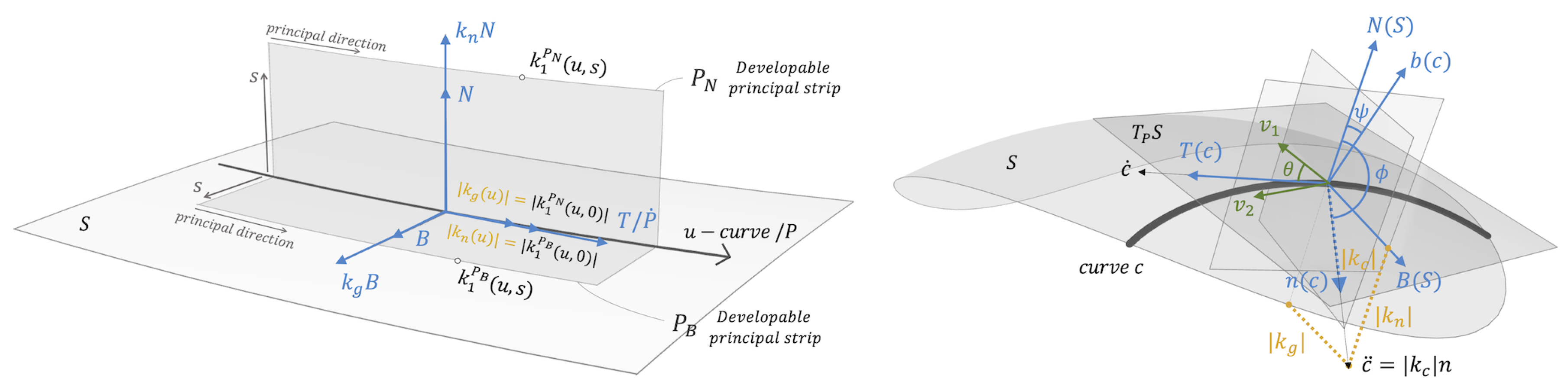
To end the section, we discuss strips along curves in CPA MS-patches, refer to [8,31]. Let c be a curve in a surface S, with its Frenet frame and its Darboux frame, its curvature and torsion, its geodesic curvature and torsion, and its normal curvature, then:
Let be the angles between and between , while be the principal curvatures of S with their principal directions and the angle between , as seen in Figure 12, then:
Furthermore, recall that a geodesic curve is one for which vanishes identically, an asymptotic curve is one is for which vanishes identically and a principal curve is one is for which vanishes identically.
Proposition 2.4.
Consider a strip along a curve c in S with for . Then, is developable if and only if c is principal, moreover, if this is the case, is a principal patch.
Let and c be as in Proposition (2.4), then that one of the principal curvatures of is zero, while the other one denoted is associated to the principal direction tangent to t-curve (of ). We then have:
Lemma 2.5.
At the level , the principal curvature is related to of the curve c by:
In fact, also for generic levels , the principal curvature is related to as shown next.
Proposition 2.6.
For the two particular cases:
Let us now focus on our initial setting where the surface S is a CP MS-patch with its corresponding CA MS-patch, given by Relation (4). In particular, the -curves are principal, the -curves are asymptotic and whenever either are a symmetry axis, they are also geodesics. By similarity, we will focus only on the principal u-curves and asymptotic x-curves given by:
Since has vanishing , it follows from Equation (11)(2) that the angle (hence ) is constant equal to (or ). From other side, since the surface is minimal, we get and the asymptotic directions bisecting the principal directions, hence the angle is constant equals . We have therefore proved that:
Lemma 2.7.
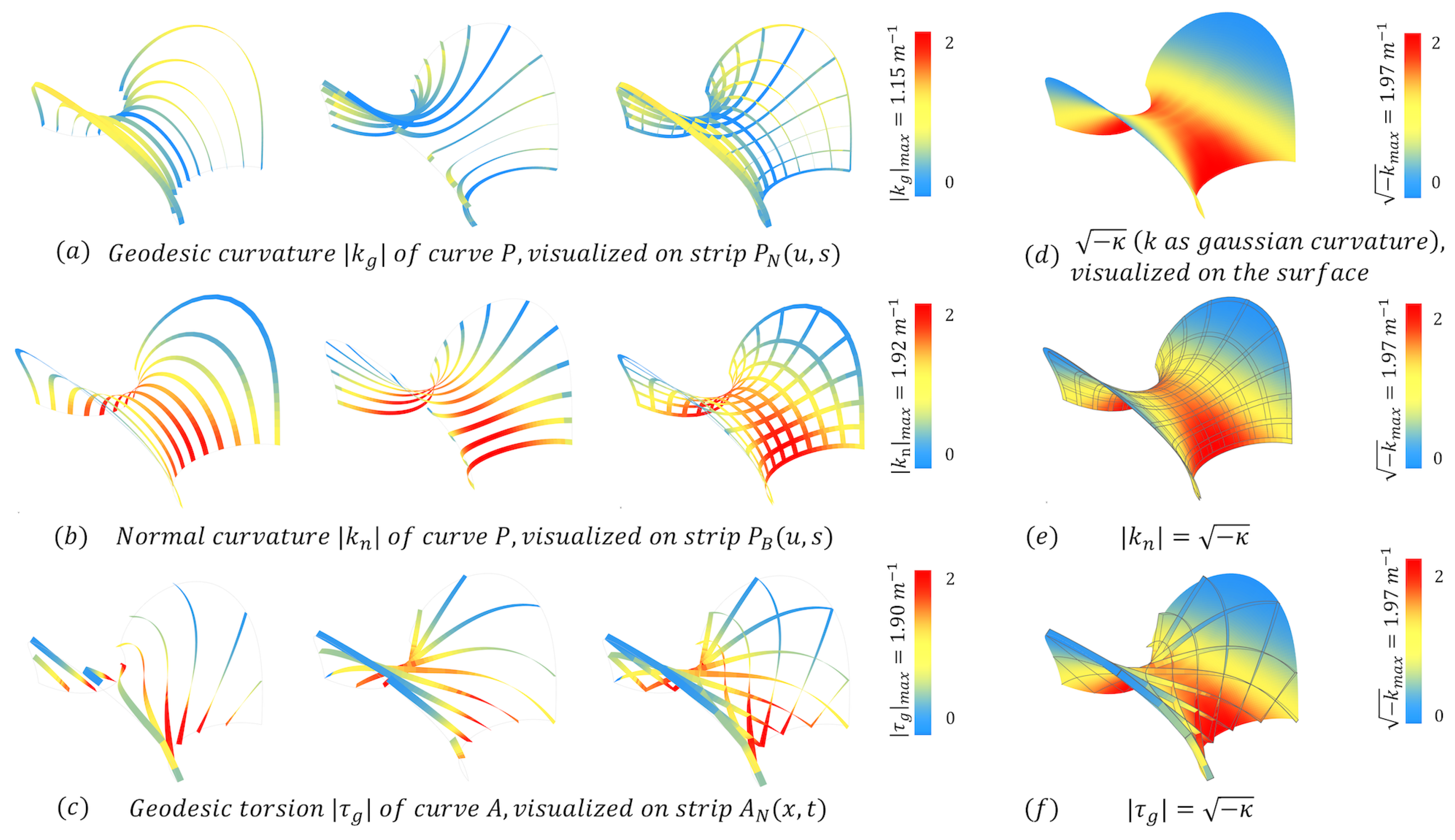
The geodesic torsion for every asymptotic curve for all fixed , coincides with its torsion and is totally determined by the Gaussian curvature of the MS at , that is
Next, for any real constants , we define the strips:
Note that, when we will denote simply by , while when we will denote it by and similarly for (refer toFigure 1). Finally, it follows from the fact that, the network curve is principal and the surface is minimal, that . Then, by Propositions (2.4) and (2.6), we have that:
Corollary 2.8.
The strip is a developable principal strip and principal curvatures of are:
3. Morphological Analysis of Shape and Configuration Variants
In Section 2, we gave the geometric tools necessary for the generation and transformation of the CPA MS-patches. In this section, we will use these tools to define the Space of Variants, (i.e. Morphological design options arising CPA MS-patches). In an more intuitive sense, in this section we will “translate” the geometry into architectural morphology. In view of the structure introduced in Section 2, we will also classify the morphological investigation in an analogous manner, with the emphasis on the design interpretation of the variations. More concretely, we will formulate the morphological exploration in terms of what we will call the degrees of Design Freedom (or DF). These DF will follow a sequential logic: DF-1, DF-2, DF-3, DF-4, refer to [1] and [2].
Clearly, the levels of DF start at the choice of the holomorphic function . Now since there are infinitely many holomorphic functions, we have an infinity of choices. However, as was stated above, we will limit ourselves here to the six-types that were shown in Figure 4. Our goal in this section is to illustrate what kind of shape variations can arise from varying these parameters DF-1, deforming the MS (DF-2, DF-3) and changing different grid configuration (DF-4). For the sake of clarity and good illustration of the method, we will fix one choice of holomorphic function and use the CPA MS-patches arising from it as the basis surface patches used for the morphological exploration. To this end, let holomorphic function be:
This will give rise to the conformal patch on the unit shphere defined by with as in (3), given by:
with conformal factor given by:
Using above as inputs and integrating the differential Systems (2), will thus yield the CPA MS-patch , admitting a Module-patch domain:
with given respectively by the expressions:
3.1. Shape and Configuration Variants
We can now construct a parameterized search space (i.e. the space of variants), based on the DF’s.
3.1.1. Shape Variants from Holomorphic Function
The first part of the DF-1, is the choice of . Here, we choose Sinus-type, so let us now focus on the variation of parameters. It can be clearly seen that the (real) parameters introduced in Expression (16) of also appear in the resulting Expressions of the CPA MS-patches . In other words, we have a 3-parameters family of CPA MS-patches pairs, all of which have the desired patch properties and Module-patch domain. More precisely, for any values of parameters the resulting pair form CPA MS-patches with X conformal principal and conformal asymptotic. This is clearly illustrated in Figure 6 and Figure 6 where varying parameters produce (continuous) deformations of the resulting MS-patches which can be used for morphological variation.
3.1.2. Shape Variants from Bonnet Transformation
The second level of design freedom DF-2 is provided by the application of the Bonnet transform defined by Relation (8). As explained in Section 2.3, the Bonnet transform, does not preserve the PA networks and thus Module-patch structure is lost, as seen in Figure 7. However, all variants are conformal MS-patches of equal area, thus, defining a search space of variants having equal material amount, among which an optimal one can be chosen with respect to a design criterion, refer to Section 3.2.
3.1.3. Shape Variants from Goursat Transformation
The third level of design freedom DF-3 is provided by the application of the Goursat transform defined by Relation (9). As explained in Section 2.3, all the are CP MS-patches and the are CA MS-patches, as seen in Figure 7. This allows us to have a continuous search space of variants having the same fabrication advantages, refer to Section 1, among which an optimal variant can be chosen with respect to a design criterion, refer to Section 3.2.
3.1.4. Configuration Variants for Structural Elements
As previously mentioned, DF-1, DF-2, and DF-3 represent shape-related variable spaces. Once the shape parameters are determined, the structure’s form is fixed. By defining these parameters across the three layers, we achieve the desired parameterized minimal surfaces. Building on this foundation, we can introduce additional design options: configuration types and configuration distribution to meet specific requirements.
• Configuration types: These are determined by selecting strips (with zero thickness) generated from principal or asymptotic parameterizations, or their combinations, and defining cross-sectional dimensions to get appropriate laths (with non-zero thickness). Thanks to the mathematical model established in Section 2.4, we can parametrically construct three types of strips on the surface: Normal principal strip , side principal strip , and normal asymptotic strip , using Equations (14). Here, we present eight feasible configuration types, as shown in Figure 8. For example, choosing an asymptotic network will naturally give rise to a grid configuration design . If enhancing the overall buckling resistance is considered, then the configuration can be selected or the arrangement order can be changed to form a configuration. Additionally, without requiring a strict correspondence between asymptotic and principal networks (refer to Section 2.2.1), adjusting the grid densities of asymptotic and principal parameters separately can result in configurations similar to reciprocal structures as . On the other hand, choosing a principal network will naturally give rise to a grid configuration of . Moreover, it can also generate a configuration from the same principal curves. Observe that type of configuration has a structural advantage stemming from the T-section beams that are made from planar members, as explained in Section 2.4. Alternatively, adding small cross-sectional asymptotic strips as bracing can form a configuration, or maintain the T-section members and combine with to form the configuration. Naturally, more configurations can be chosen according to projects requirements.
• Configuration distribution: Another design freedom is the ability to adjust the grid density of PA networks arising from of CPA MS-patches , refer to Figure 9. This is achieved through a reparameterization using monotonous functions (i.e. without inflection points) such that
This reparameterization can enrich the overall design, as it will allow for more uniform distribution of the principal and asymptotic networks on the MS. The downside is that we lose the correspondence between these two networks described in Section 2.2.1. In view of the above, this design freedom is applicable only if one does not intend to make use of the principal-asymptotic correspondence in their design, for example the case study presented in Section 4. It is also worth mentioning that a visual re-mapping tool that simulates the effects of the functions can be achieved using the graph-mapper and number-remapping tools in Grasshopper. These were used in uniformizing the distribution of the principal network configuration laths configuration gird) and the asymptotic network configuration laths configuration grid) shown in Figure 9. Note that, so far we articulated the space of variants based on the four DF, in the following we will show how to select variants that have better fitness with respect to architectural and structural criteria.
3.2. Selection of Variants
In the previous subsection, we constructed a parameterized space of variants, where every variant contained in it, satisfies geometric properties associated to fabrication advantages. Let us now show how to carry out selection processes of the variants based on two criteria: architectural and structural.
3.2.1. Architectural Criteria
We consider two examples of quantifiable criteria.
• Size and Orientation: Here, the fitness of a variant is tested using a bounding-box (based on the project’s dimensions) and placed on the MS, through scaling (size) and 3D-rotation (orientation). Analyzing whether (a portion) of the variant can provide the basis for the project’s design.
• Spatiality: Another architectural criterion is “spatiality”, referring to the usable space defined by the area having a vertical distance to the surface greater than a certain constant (typically an average human height), as shown in Figure 10. Here, the fitness of a variant is tested by its “spatiality ratio” where is the usuable area and is the total (foot print) area under the MS. By comparing the spatiality-ratios of different variants (as the parameters vary), designers can gain insights into which designs are more spatially efficient and better suited to the context.
3.2.2. Structural Criteria
We consider two examples of structural criteria.
• Active-bending / twisting stress: Note that, to put planar material laths in their designed curved form, they will require pre-bending / twisting, hence, they will experience the so-called active-bending / twisting stress level. Let us briefly recall some concepts from classical material mechanics theory, refer to [15]. Consider a curve in a surface, being the centered base curve of a ruled strip, giving rise to a material lath. We can then consider that curve to be the axial curve (of the lath) and the material frame of the lath to be aligned with its Darboux frame (with respect to the surface). The “curvature” of the lath is then given by the curvature of the axial curve and the “torsion” of the lath is given by the torsion of the axial curve. Next, let M be the bending moment, T the torque, the material’s elasticity modulus and the shear modulus. Furthermore, let I be the cross-sectional modulus, the normal stress and the shear stresses. It then follows that we have:
Now, since the material is fixed then the moduli are constant and by using the same cross-sections for the whole model, the cross-section modulus I is also constant. It then follows, from the linearity of Relations (18) that the curvature / torsion are directly proportional to the bending / shearing stresses. Building on this foundation, we conduct a further analysis of the curvature and torsion characteristics of different types of strips. As discussed in Section 3.1.4, our focus is on three types of laths arsing from strips. These are laths from with axial principal curve and laths from with axial asymptotic curve , defined by Equations (14) in Section 2.4.
Remark 3.1.
In view of Section 2.4, we observe that:
- (i)
- By Corollary (2.8), laths experience only bending and by Lemma (2.5) we have that:
- (ii)
- Laths experience twisting determined by of A and by Lemma (2.7),
- (iii)
- By Equation (18) and (i),(ii), we have that:
It follows directly from Remark (3.1), the active-bending / twisting stresses levels (of laths ) are totally determined by evaluating the curvature / torsion (of the axial curves ), as depicted in Figure 11. Once the cross-sectional size and material properties are defined, the assembly-induced stress can be calculated by Equations (19). It is important to note that these relations are valid only when the material is within its elastic range.
• Stiffness: Grid stiffness is a crucial indicator for assessing a grid’s structural performance throughout its service life. The maximum displacement of a grid under a specific load clearly demonstrates the stiffness of the target structure. Here, we will evaluate stiffness performance under self-weight while the varying parameters, as seen in Figure 10. The results indicate that, with the same cross-section and load conditions, the structural stiffness ranks as follows:
This parametric analysis allows for the identification of shape parameter ranges that enhance structural efficiency, aiding designers to quickly pinpoint more effective structural forms. However, the structural analysis tools used has not yet been integrated into a unified design workflow with the aforementioned guidelines. This integration could be the subject of future research. Additionally, we can extend this research to compare and analyze the performance of different cross-section forms, as shown in Figure 8.
Figure 12.
Left: Laths from with common axial curve P. Right: Decomposition of into , .
4. Case Study
In this section, we present a real-life design case to demonstrate the efficiency and usability of the method.
• Introduction to the case: As part of the Master’s course "Exploration" at the ENSAPL (École Nationale Supérieure d’Architecture et de Paysage de Lille), a workshop was conducted in 2024. This workshop included two phases: design and fabrication. During the design phase, groups of students explored architectural applications of CPA MS-patches, guided by our design algorithm and workflow, with the aim of creating a suspended structure in the atrium of the ENSAPL. The final (modular) design utilized the symmetry and periodicity of the CPA MS-patches, simplifying fabrication by repeating the same module-patch four times to yield the entire structure.
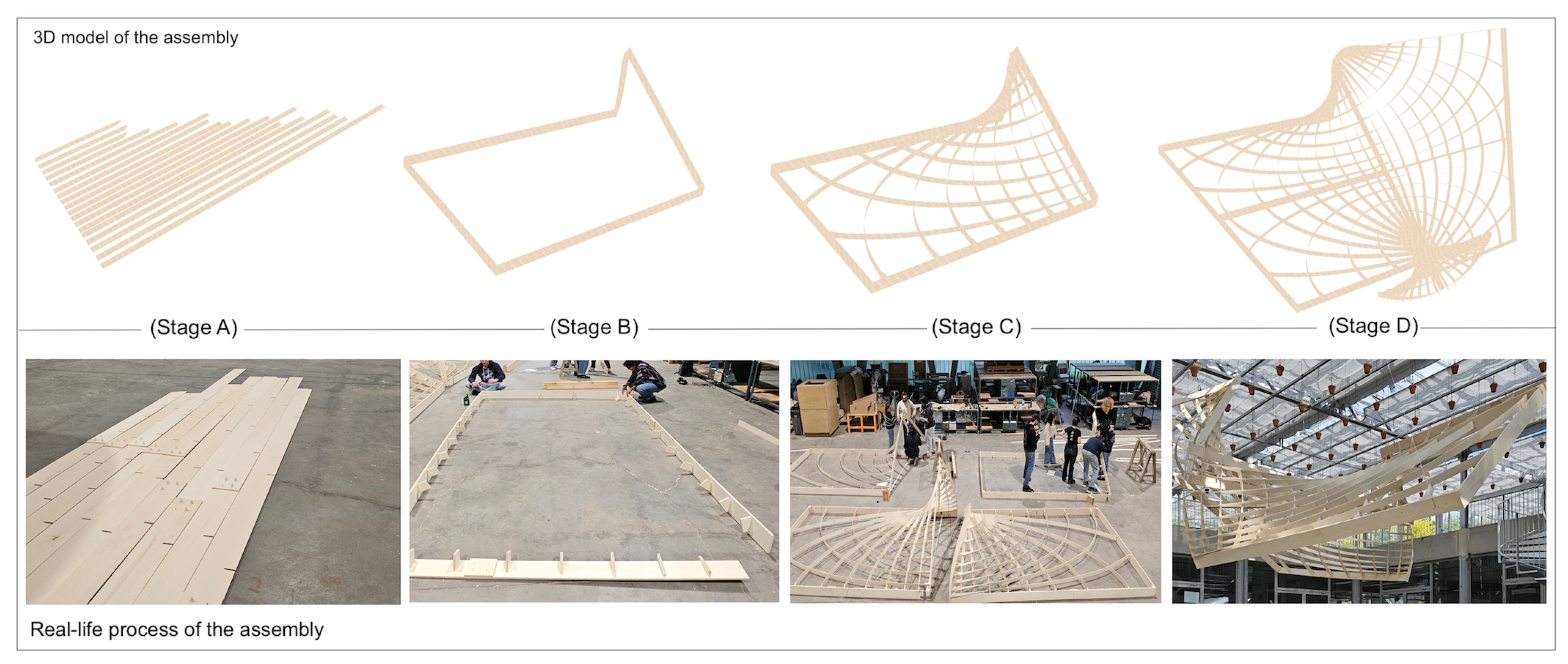
• Detailed steps and result: For the design, we selected a sinus-type CA MS-patch with a Goursat transform, an laths configuration with redistribution to ensure uniform grid spacing. We tested sample laths at the points of maximum assembly stress, curvature, and torsion to ensure that the material remained within its elastic range under target conditions. Next, laths (5mm thick) were cut and assembled into the (four repeating) modules. Each module, measured approximately 3.5m by 2m with a height of 1.5m, designed with a rigid frame and connectors for simplified assembly. The assembly sequence followed the results of the active-bending/twisting stress analysis, from high-stress to low-stress laths. The construction of a single module took approximately six hours (with four people working on it), and the entire (four modules) structure was completed within two working days. The most challenging aspect was suspending the modules from the atrium ceiling at a height of 6m, requiring precision and careful coordination.
Figure 13.
Top: 3D model of assembly steps. Bottom: Real-life assembly steps.
5. Workflow
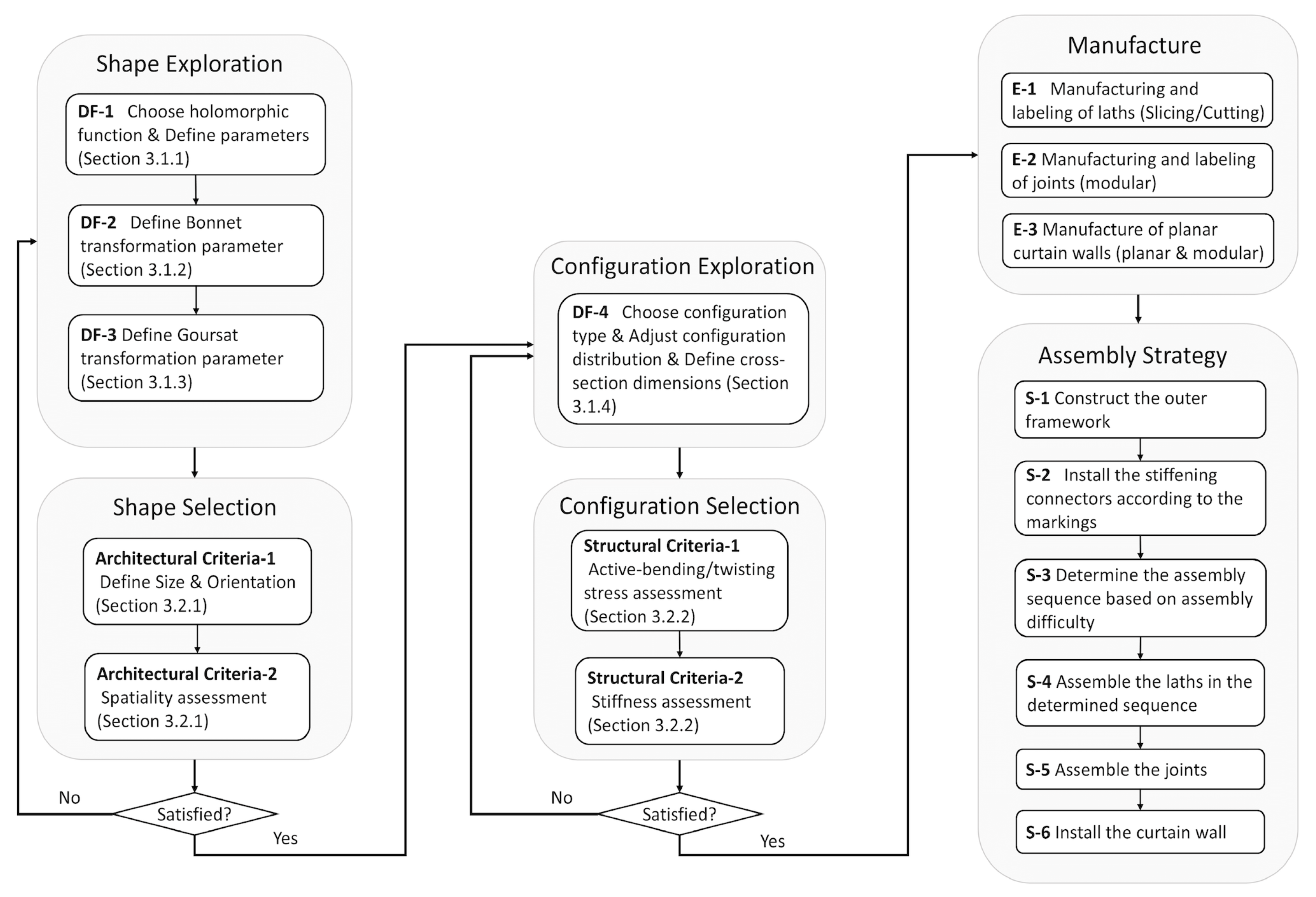
In this section, we provide an overview of the method’s workflow, the process is divided into three stages:
• Shape exploration and selection:
- -
- Exploration: The first step in any new design is to explore the potential shape design space. Based on the geometric methods established in Section 2, there are three degrees of freedom (DF) at the geometric shape level: DF-1, DF-2, and DF-3 (refer to Section 3.1). DF-1 allows for the selection of different initial shapes using various holomorphic functions, as shown in Figure 4. Designers can choose functions: Square-type, Sinus-type or Cosinus-type for single / double periodicity or Mobius-type for more complex shell structures. After selecting a holomorphic function, further adjustments can be made by modifying its patch-parameters . DF-2 offers the Bonnet transformation, which can convert the CP MS-patch X to its adjoint CA MS-patch, with intermediate MS-patches are only conformal, however all instants are isometric. DF-3 introduces the Goursat transformation, which retains the properties of both CP MS-patch and CA MS-patch.
- -
- Selection: With a diverse design space (i.e. space of variants) established through DF-1, DF-2, and DF-3, the next step is shape selection based on architectural criteria. The first criterion is size-orientation, ensuring that geometric shapes are scaled and oriented to fit project specifications, particularly for boundary support. The second criterion is spatiality, note that, while freeform surfaces offer aesthetic variety, they can create unusable spaces. Variants are filtered using the spatiality-ratio from Section 3.2.1, favoring those with higher usable space ratios.
• Configuration exploration and selection:
- -
- Exploration: Once the shapes are determined, we move to detailed structural design. Using the geometric methods from Section 2.4, we can efficiently identify the principal and asymptotic parameterized networks of minimal surfaces, enabling the construction of various configuration types Figure 8. By adjusting intervals, grid density can be modified to explore different configurations that meet diverse project needs Figure 9.
- -
- Selection: Here, designers can initially filter options based on design intent and joint fabrication complexity. The next step is a more detailed selection based on structural performance. The first criterion, "Active Bending and Twisting Stress," involves locating maximum stress points using curvature analysis from Section 3.2.2. By defining material and cross-section, stress magnitude can be quickly calculated and controlled by adjusting cross-section dimensions. The second criterion, "Stiffness," uses third-party analysis tools to evaluate mechanical performance under various conditions, allowing for parametric comparisons to optimize design parameters.
• Manufacturing and assembly strategy:
- -
- Manufacturing: We have three main produced elements types: (E-1) laths, (E-2) modular joints, and (E-3) flat curtain walls. (E-1) include laths unrolled into without deformation to flat pieces and laths unrolled into straight bands for material cutting. (E-2) require detailed design based on the configuration (although not treated here). Finally, for (E-3) we can fill the configuration with planar quads and add boundary stiffening connectors.
- -
- Assembly strategy: Note that, even though elastic gridshells simplify processing and manufacturing, they have new assembly challenges. Unlike typical freeform structures, bending-active structures achieve their shape through bending and twisting straight or planar beams, which generates normal and shear stresses during assembly. Thus, a precise assembly strategy is essential. References from Eike Schling, Zongshuai Wan, and others offer valuable insights [30]. Their method involves deformations from a curved surface to a plane. However, when these deformations are not mathematically controlled, flattening a curved gridshell can induce significant joint stress and plastic deformation in laths [35], which must be avoided. To prevent plastic deformation, large surfaces are often divided for assembly, increasing complexity and affecting structural coherence.
Figure 14.
Workflow.
Building on these studies, we propose a rational assembly step-by-step method, as illustrated in Figure 13:
- -
- Step-1: Assemble boundary conditions, such as joint constraints, fixed outer frame.
- -
- Step-2: Install boundary connectors.
- -
- Step-3: Design the assembly sequence, prioritizing laths with the highest twisting stress.
- -
- Step-4. Following the sequence, connect one end of the lath to the stiffener, insert intermediate joints.
- -
- Step-5: Install modular connectors.
- -
- Step-6: Install planar curtain wall components.
6. Conclusions
In this work, we enhanced the design and construction efficiency of CPA elastic gridshells base on MS, for sustainable building applications by developing a parametric design algorithm. This algorithm integrates modular construction with a rich design space, accommodating diverse shapes, laths configurations, and beam section designs, including deployable T-shaped sections. It simplifies the design process by providing precise geometric-based analysis of assembly stresses, like active-bending / twisting, making complex freeform surface designs more accessible to designers. The algorithm streamlines the design process by eliminating the need for recalculations with each parameter change, ensuring that construction and mechanical performance considerations are integrated from the start. It establishes quantitative standards for evaluating building performance, making it a mature tool for guiding architectural geometry decisions throughout the design cycle. As was seen the algorithm presented, focused only on MS, as its basis geometric theory focused only on conformal principal and asymptotic patches on MS. However, this should not be seen as a limitation, since this algorithm presents a form of pre-rationalized approach to designing gridshells, where the rationalization is based on a pre-defined geometric properties. Hence, this algorithmic method can be easily adapted to other geometric theory of other types of surfaces and networks of curves, with other favorable fabrication advantages. Now, expanding the scope of application of our method, is definitely motivation for our future research work in architectural geometry. For the moment, we believe the algorithm provides a strong foundation for advancing MS elastic gridshell design and construction. Future improvements could focus on: exploring the application of geometric theories of other surfaces types and gridshell construction, conducting mechanical experiments to gather data on torsion angles and bending radii for various materials, analyzing the impact of active-bending / twisting on structural efficiency and buckling, comparing with axial-force-dominated freeform surface gridshells; studying the long-term performance of elastic gridshells; examining different joint designs and overall structural efficiency through experimental analysis, and developing an integrated mechanical model that includes active-bending / twisting stresses under self-weight and external loads for comprehensive analysis. In ending, we hope that our presentation of the methods was clear enough (specially for non-mathematical readers) and that it provided ready-to-use tools for designers.
Acknowledgments
This research was supported by multiple grants. Author Xinye Li was supported by China Scholarship Council (CSC). Author Elshafei, A. was partially financed by Portuguese Funds through FCT (Fundação para a Ciência e a Tecnologia) within the Projects UIDB/00013/2020 and UIDP/00013/2020.
Appendix A. Mathematical Proofs
We provide here proofs for the used results.
• Proof of Lemma (2.2): Note that, since and we have that:
The first fundamental form in the -coordinates is , thus in the -coordinates it is with , making Y conformal. The second fundamental form in the -coordinates is , thus in the -coordinates it is with , making Y asymptotic. The converse arguments are clearly analogous.
• Proof of Theorem (2.1): We prove two items separately:
- -
-
Item (1): It follows from Section 2.2.2 that to show that a coordinate curve or is a symmetry axis, it suffices to show that it is image by N is contained in a great circle. Consider the function of the six-types, we observe that:Note that since parameter c only shift the u-domain in Sinus, Cosinus-types, it is set to zero. Recalling the spherical images are given by , and that the conformal mapping sends radial lines through the origin to great circles (vertical meridians) in , Item (1) is thus proven.
- -
-
Item (2): In view of the discussion in Section 2.2.2, to determine the periodicity of the six types, it suffices to compute the period vector given by Equation (7), the contour integral of loops around punctures. To this end, we determine the Weierstrass data and the punctures (singularities of the functions ) for each of the six types:Using the above data to compute the period vectors given by Equation (7) of the form for X and for , yielding the statement of Item(2).
• Proof of Proposition (2.4): Observe that and the normal equals , hence the Gaussian curvature will vanish identically if and only if , or equivalently aligns to or (i.e. to ). Now the vectors cannot be colinear, since otherwise will not form a frame. There follows that, if and only if are aligned. Now since the constants are not both zero, substituting the expressions for from Equations (10) in that of yields are aligned if and only if . This is equivalent to being principal. Finally, the vanishing of is equivalent to the vanishing of the coefficient f, making the strip conjugate, while, the alignment of , results in the vanishing of the coefficients F, making the strip orthogonal.
• Proof of Lemma (2.5): Since is a principal patch, its principal curvature is given by the quotient of the fundamental coeffiecients and . By direct computation of the coefficients, we obtain
in particular, at the principal curvature is given by
Since and , then , moreover, we have with A the T-component function. Putting these in the above expression for we obtain the Formula (12). Finally, the second statements follow immediatly by putting and then putting .
• Proof of Proposition (2.6): We use the expressions of the coefficients and the decomposition of (in the Darboux frame) involving as seen in the proof of Lemma (2.5). Now, for we have that , therefore and , it then follows that
While, for we then have that , therefore and , it then follows that
The result then follows immediately be taking quotient in both cases.
References
- Abdelmagid, A. , Elshafei, A., Mansouri, M., and Hussein, A. (2022). A design model for a (grid)shell based on a triply orthogonal system of surfaces. In Towards Radical Regeneration: DMS Berlin 2022. Springer.
- Abdelmagid, A. Tosic, Z., Mirani, A., Hussein, A., and Elshafei, A. (2023). Design model for block-based structures from triply orthogonal systems of surfaces. Proceedings of Advances in Architectural Geometry, DeGruyter, pages 165–176.
- Bobenko, A. Hoffmann, T., and Springborn, B. (2006). Minimal surfaces from circle patterns: Geometry from combinatorics. Ann. of Math., 164:231 – 264.
- Bobenko, A. and Pinkall, U. (1996). Discrete isothermic surfaces. J. reine angew. Math., 475:187 – 208.
- Bonnet, O. (1867). Mémoire sur la théorie des surfaces applicables. J. Ec. Polyt., 42:72–92.
- Christoffel, E. (1867). Ueber einige allgemeine eigenschaften der minimumsflächen. Crelle’s J., 67:218 – 228.
- Cisneros, A. S. R. Aikyn, A., Kilian, M., Müller, C., and Pottmann, H. (2024). Approximation by meshes with spherical faces. ACM Trans. Graphics, 43(6). Proc. SIGGRAPH.
- Darboux, G. (1896). Leçons sur la théorie génerale des surfaces. Gauthier-Villars.
- Dierkes, U. Hildebrandt, S., and Sauvigny, F. (1992). Minimal surfaces. Springer, Berlin, Heidelberg.
- Douthe, C.; Mesnil, R.; Orts, H.; Baverel, O. Isoradial meshes: Covering elastic gridshells with planar facets. Automation in Construction 2017, 83, 222–236. [Google Scholar] [CrossRef]
- Eisenhart, L. A Treatise on Differential Geometry of Curves and Surfaces; Ginn and Company: Boston, 1909. [Google Scholar]
- Glymph, J. , Shelden, D. R., Ceccato, C., Mussel, J. W., and Schober, H. (2004). A Parametric Strategy for Freeform Glass Structures Using Quadrilateral Planar Facets. ACADIA proceedings.
- Goursat, E. (1887). Sur un mode de transformation des surfaces minima (1,2). Acta Math., 11:(135–186), (257–264).
- Gray, A. bbena, E., and Salamon, S. (2006). Modern differential geometry of curves and surfaces with Mathematica. 3rd Edition. Chapman & Hall/CRC.
- Hibbeler, R. (2016). Mechanics of Materials. Pearson.
- Kilian, M. , Cisneros, A. S. R., Müller, C., and Pottmann, H. (2023). Meshes with Spherical Faces. ACM Transactions on Graphics, 42, 1–19.
- Liu, Y. , Pottmann, H., Wallner, J., Yang, Y., and Wang, W. (2006). Geometric modeling with conical meshes and developable surfaces. ACM Tr., Proc. SIGGRAPH, 25, 681–689.
- Mansouri, M. Abdelmagid, A., Tosic, Z., Orszt, M., and Elshafei, A. (2023). Corresponding principal and asymptotic patches for negatively-curved gridshell designs. Proceedings of Advances in Architectural Geometry, DeGruyter, pages 55–67.
- Mesnil, R. and Baverel, O. (2023). Pseudo-geodesic gridshells. Engineering Structures, 279:115558.
- Mesnil, R. , Douthe, C., Baverel, O., and Léger, B. (2018). Morphogenesis of surfaces with planar lines of curvature and application to architectural design. Automation in Construction, 95, 129–141.
- Montagne, N. Douthe, C., Tellier, X., Fivet, C., and Baverel, O. (2022). Discrete voss surfaces: Designing geodesic gridshells with planar cladding panels. Automation in Construction, 140:104200.
- Pellis, D. and Pottmann, H. (2018). Aligning principal stress and curvature directions. In Hesselgren, L., Kilian, A., Malek, S., Olsson, K.-G., Sorkine-Hornung, O., and Williams, C., editors, Advances in Architectural Geometry, pages 34–53. Klein Publishing Ltd.
- Pellis, D. and Pottmann, H. (2024). The geometry of principal symmetric structures. Structures, 60:105972.
- Pellis, D. , Wang, H., Kilian, M., Rist, F., Pottmann, H., and Müller, C. (2020). Principal symmetric meshes. ACM Transactions on Graphics, 39.
- Pillwein, S. , Leimer, K., Birsak, M., and Musialski, P. (2020). On Elastic Geodesic Grids and Their Planar to Spatial Deployment. ACM Transactions on Graphics, 39, 12.
- Pillwein, S. and Musialski, P. (2021). Generalized Deployable Elastic Geodesic Grids. ACM Transactions on Graphics, 40, 15.
- Pottmann, H. Asperl, A., Hofer, M., and Kilian, A. (2007a). Architectural Geometry. Bentley Institute Press, Pennsylvania.
- Pottmann, H. , Liu, Y., Bobenko, A., Wallner, J., and Wang, W. (2007b). Geometry of multi-layer freeform structures for architecture. ACM Tr., Proc. SIGGRAPH, 26, 1–11.
- Schling, E. (2021). Asymptotic Building Envelope - combining the benefits of asymptotic and principal curvature layouts. In Proceedings of the 26th CAADRIA Conference. CUMINCAD.
- Schling, E. and Wan, Z. (2022). A geometry-based design approach and structural behaviour for an asymptotic curtain wall system. Journal of Building Engineering, 52, 104432.
- Spivak, M. (1999). A Comprehensive introduction to differential geometry. Publish or Perish.
- Tang, C. Sun, X., Gomes, A., Wallner, J., and Pottmann, H. (2014). Form-finding with polyhedral meshes made simple. ACM Trans. Graphics, 33(4). Proc. SIGGRAPPH.
- Tellier, X. (2022a). Bundling elastic gridshells with alignable nets. Part I: Analytical approach. Automation in Construction, 141:104291.
- Tellier, X. (2022b). Bundling elastic gridshells with alignable nets. Part II: Form-finding. Automation in Construction, 141:104292.
- Wan, Z. and Schling, E. (2023). Structural behaviour of an asymptotic curtain wall stiffened with lamella couplings. Journal of Constructional Steel Research, 207:107938.
- Wang, B. Wang, H., Schling, E., and Pottmann, H. (2023). Rectifying strip structures. ACM Trans. Graphics, 42(6):256:1–256:19. Proc. SIGGRAPH Asia.
- Weber, M. (2001). Classical minimal surfaces in euclidean space by examples. Lec. Notes Clay Mathematical SummerSchool MSRI, Berkeley.
Figure 1.
Geometric properties of Minimal surface (MS)-patches corresponding to fabrication advantages.
Figure 1.
Geometric properties of Minimal surface (MS)-patches corresponding to fabrication advantages.
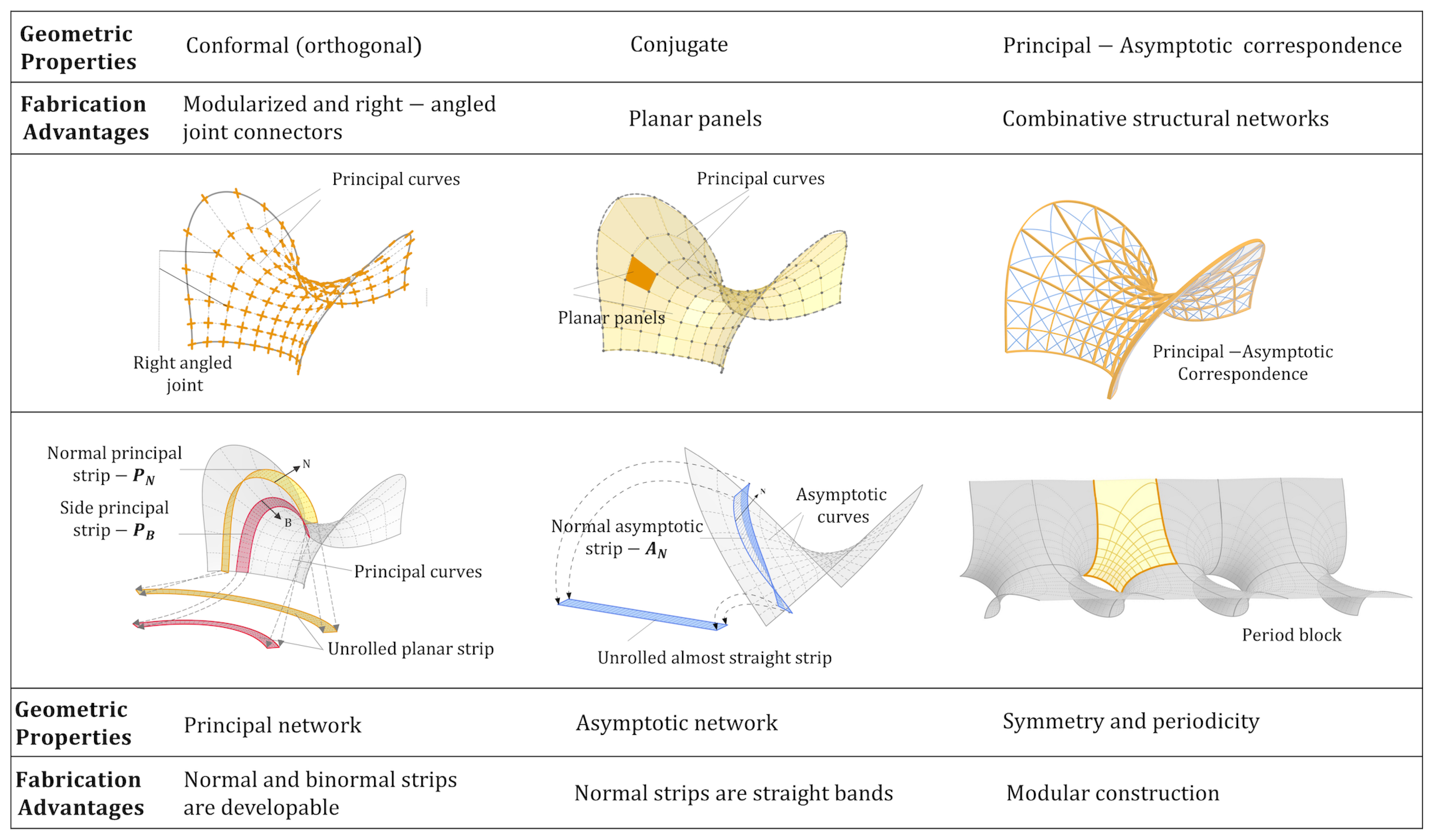
Figure 2.
Left: Reparameterization-A (corresponding PA networks). Right: Reparameterization-B.
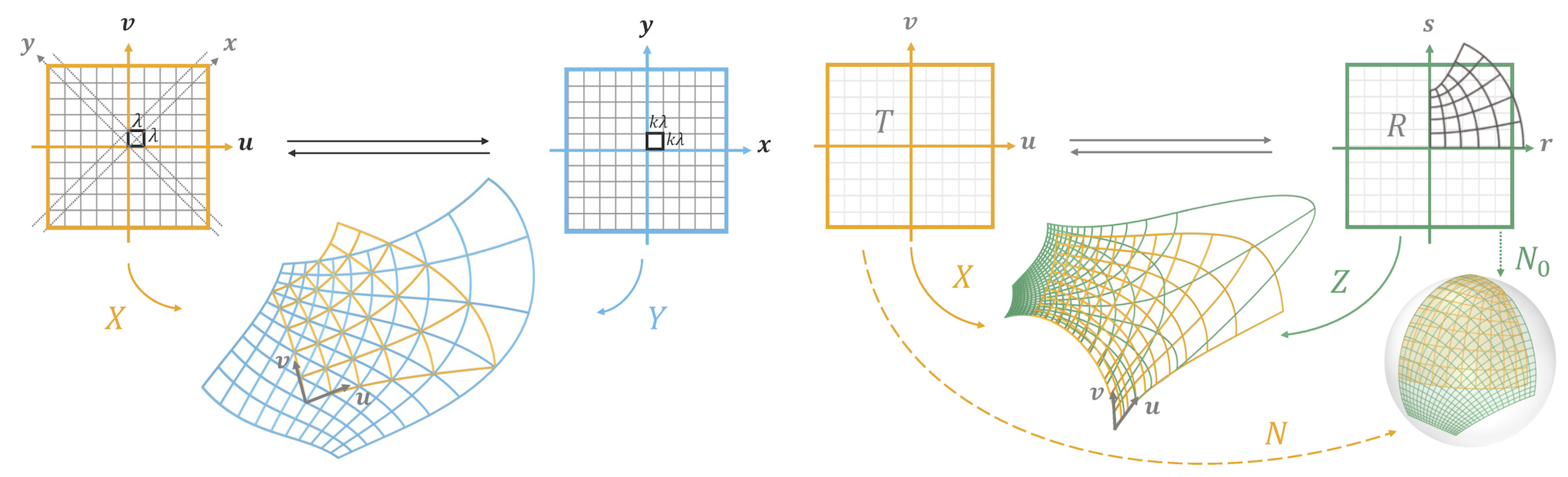
Figure 3.
Left: Symmetry axes (correspondence). Right: Periodicity.
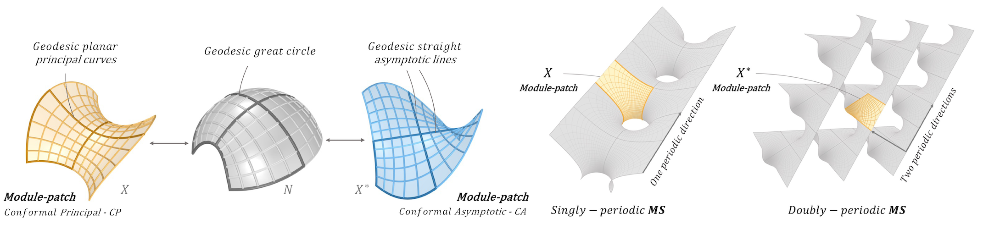
Figure 4.
The six types of the pair showing Module-patches.
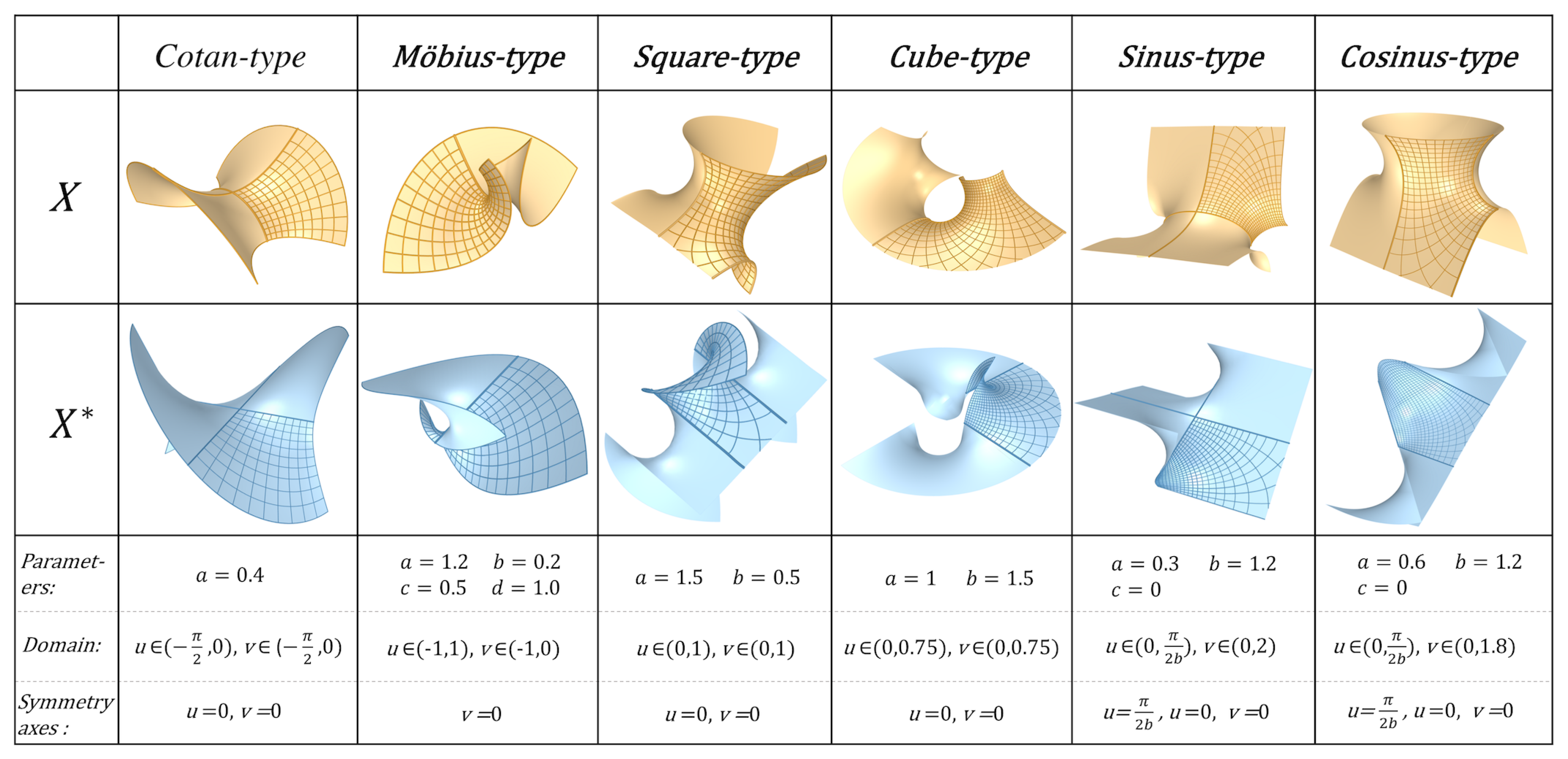
Figure 5.
Left: Bonnet Transform. Right: Goursat Transform.
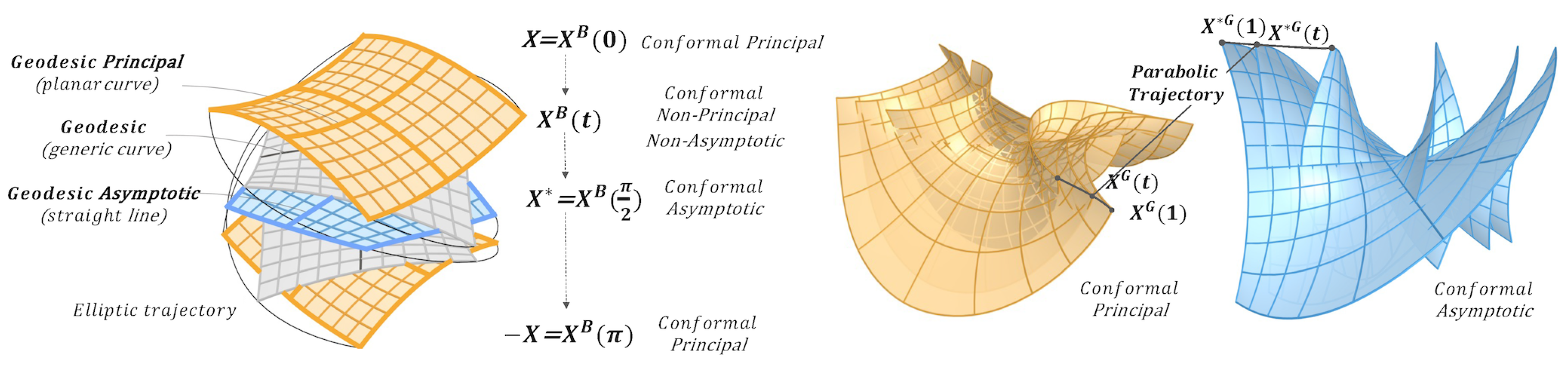
Figure 6.
CP MS-patches X (left) (right) obtained from varying .
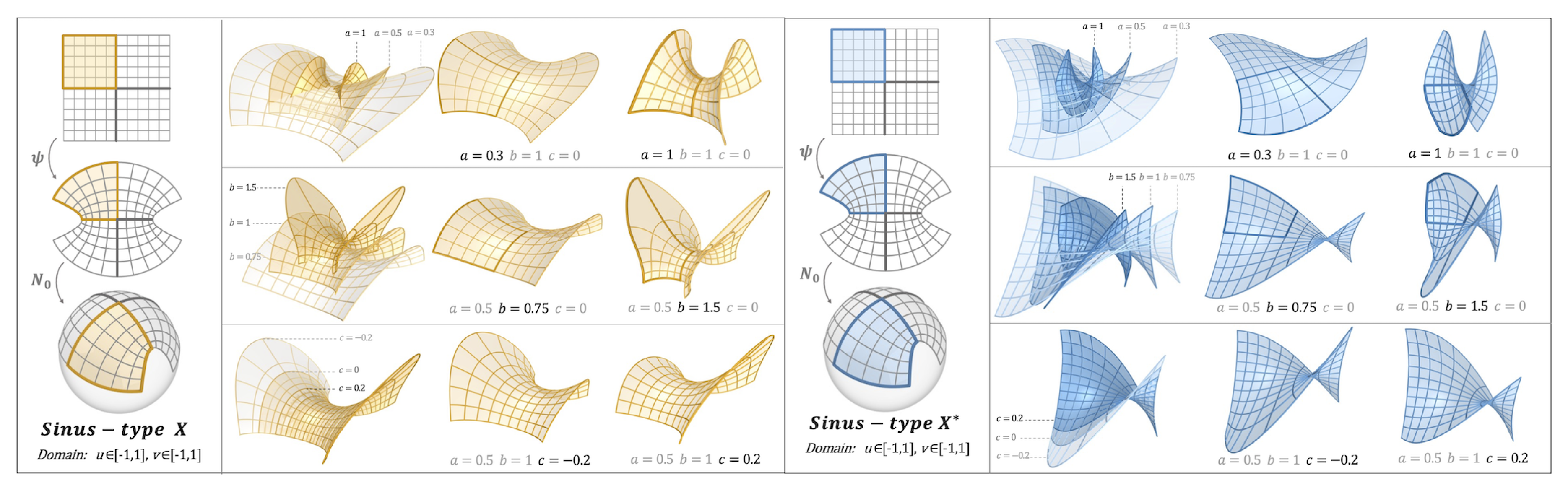
Figure 7.
Left: Bonnet transform preserving metric properties. Right: Goursat transform preserving PA patch properties.
Figure 7.
Left: Bonnet transform preserving metric properties. Right: Goursat transform preserving PA patch properties.
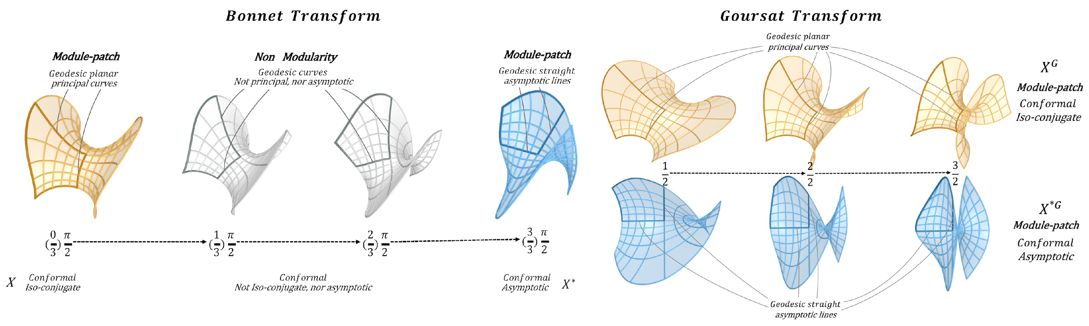
Figure 8.
Eight configurations: , : (1) a detailed view of the configuration types, (2) an overall configuration view, and (3) a simplified representation diagram.
Figure 8.
Eight configurations: , : (1) a detailed view of the configuration types, (2) an overall configuration view, and (3) a simplified representation diagram.
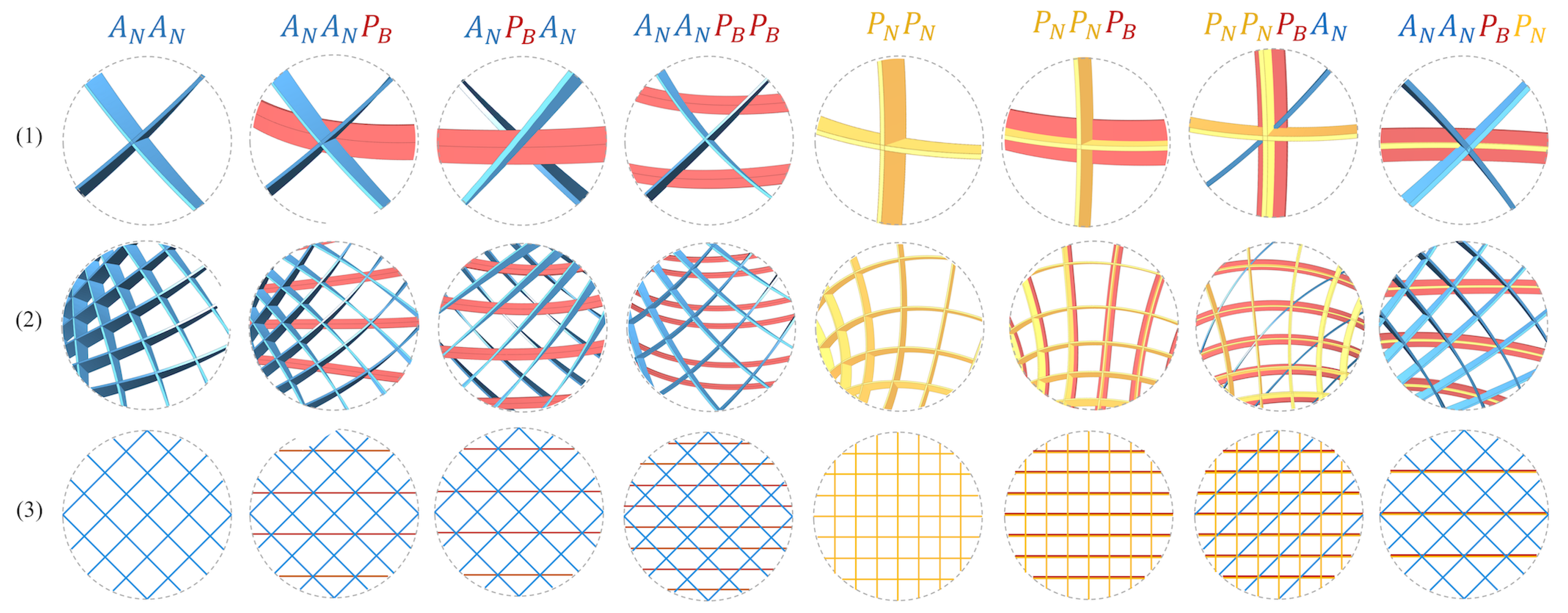
Figure 9.
Comparison of different configuration distributions: (1) PA configuration types. (2) Uniform equidistant -curves, resulting in a non-uniform grid laths distribution. (3) Non-uniform non-equidistant -curves resulting in a more uniform grid laths distribution. Note that the localized diagrams in (2) and (3) are extracted from the same region of the same surface for comparison.
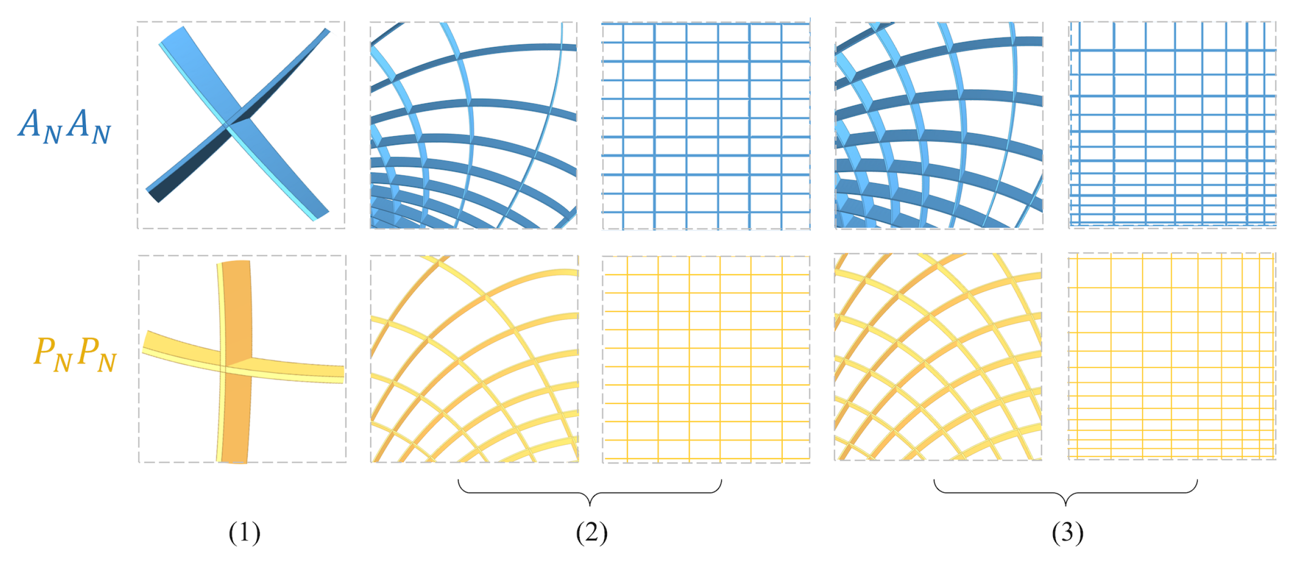
Figure 10.
(a): Analysis of spatiality ratio for a Sinus-type variant as the parameters vary. (b): Normalized stiffness of , and of their combinations under self weight.
Figure 10.
(a): Analysis of spatiality ratio for a Sinus-type variant as the parameters vary. (b): Normalized stiffness of , and of their combinations under self weight.
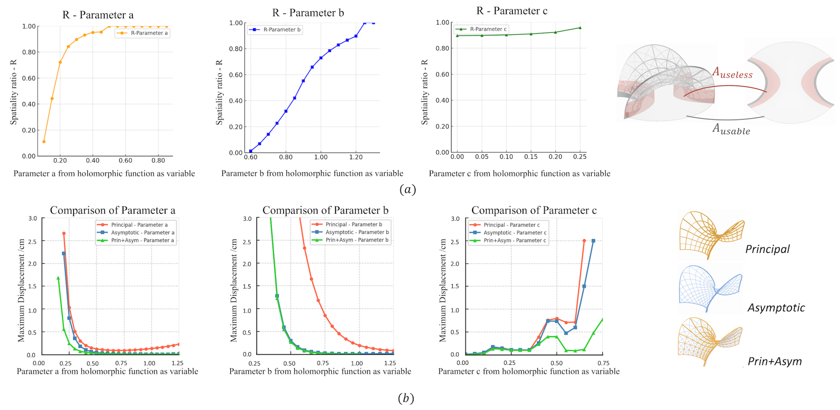
Figure 11.
Curvature analysis of the MS and curves to demonstrate the active-bending / twisting stress.
Figure 11.
Curvature analysis of the MS and curves to demonstrate the active-bending / twisting stress.
Disclaimer/Publisher’s Note: The statements, opinions and data contained in all publications are solely those of the individual author(s) and contributor(s) and not of MDPI and/or the editor(s). MDPI and/or the editor(s) disclaim responsibility for any injury to people or property resulting from any ideas, methods, instructions or products referred to in the content. |
© 2025 by the authors. Licensee MDPI, Basel, Switzerland. This article is an open access article distributed under the terms and conditions of the Creative Commons Attribution (CC BY) license (http://creativecommons.org/licenses/by/4.0/).
Copyright: This open access article is published under a Creative Commons CC BY 4.0 license, which permit the free download, distribution, and reuse, provided that the author and preprint are cited in any reuse.


