
Submitted:
07 March 2025
Posted:
07 March 2025
You are already at the latest version
Abstract
Agriculture plays a dual role in shaping biodiversity, providing secondary habitats while posing significant threats to ecological systems through habitat fragmentation and land use intensification. This study evaluates the impact of land use types on avian biodiversity in a predominantly agricultural landscape in Apulia, Italy, by analyzing 20 sites fuzzily classified into three ecosystem categories: agricultural (AGR), mixed (MIX) and natural (NAT), according to the percentage of natural cover. Biodiversity indices were calculated for each bird community observed. The abundance curves showed a geometric series pattern for the AGR communities, indicative of ecosystems at an early stage of ecological succession, and a lognormal distribution for the MIX and NAT communities, typical of mature communities with a more even distribution of species. Analysis of variance showed significant differences in richness and diversity between AGR and NAT sites, but not between NAT and MIX, which had the highest values. Logistic regression estimated the probability of sites belonging to the three ecosystem categories as a function of biodiversity, confirming a strong similarity between NAT and MIX. Finally, linear discriminant analysis confirmed a clear separation from AGR areas, as evidenced by the canonical components. The results highlight the importance of integrating high-diversity landscape elements and appropriate agricultural practices to mitigate biodiversity loss. Even a small increase in the naturalness of agricultural land would be sufficient to convert it from AGR to MIX ecosystem category, with significant biodiversity benefits.
Keywords:
farmland birds
; agroecosystem
; ecological network
; high nature value farmland (HNVF)
; high-diversity landscape features (HDLFs)
; α and β diversity
; rural landscape planning
1. Introduction
Agriculture must meet society's potentially competing demands for food, fiber and fuel, while protecting natural resources, reducing negative environmental impacts and providing regulating, supporting and cultural ecosystem services. This requires coherent rural landscape planning that can promote and facilitate the achievement of these seemingly conflicting objectives.
The great turning point in agricultural practices occurred in the second half of the 20th century and was unprecedented [1]. The so-called “Green Revolution” was a global process of technology transfer that spread around the world and greatly increased crop yields. Over the past 80 years, economic expansion and technological innovation in Europe and North America have led to a rapid and strong intensification of agriculture in an industrial direction, resulting in impressive increases in agricultural productivity [2,3]. Agriculture, with 38.2% of the EU-27's land area [4], is the dominant land use category in the European Union. Despite the fact that there are as many as 41 "agricultural" habitats listed in Annex I of the Habitats Directive [5], and despite the importance of different farming systems in maintaining biodiversity, such as extensive grazing or traditional orchards [6], industrial intensification of agriculture is recognized as a major driver of biodiversity loss and ecosystem degradation [7]. Indeed, the “non-food” ecosystem services that agroecosystems can provide, such as carbon storage, water purification, pollination, natural pest control and soil productivity pay the price for maximizing agricultural yields [8].
The expansion of cropland along with the degradation and reduction of semi-natural habitats, especially high-diversity landscape features (HDLFs) such as hedgerows, ponds, small woods, individual trees, dry-stone walls and terraces [9], deplete the local ecological network and thus threaten the connectivity of the agricultural land matrix [10]. The conservation and increase of HDLFs is therefore a major challenge in reconciling agriculture and biodiversity [11]. Natural sciences and applied ecology address these issues very clearly, while environmental policy should solve the related problems through a series of specific measures. The main EU policies affecting both agriculture and the environment include the Common Agricultural Policy (CAP), in particular through agri-environmental schemes (AES), and the EU Biodiversity Strategy 2030 (EU-BDS). These policies are complemented by the European Commission's recent proposal for a Nature Restoration Law (NRL), approved on 27 February 2023 by the European Parliament in a tight vote and finally adopted by the European Council on June 17, 2024. Several authors and also public authorities have noted that AESs do not always achieve their goals [7,12,13,14,15,16] and their effectiveness in securing biodiversity is still being debated across Europe [17,18,19,20,21,22]. The CAP 2023-2027 aims to mitigate environmental degradation and combat biodiversity loss in Europe's agricultural areas by achieving three main “green” objectives: contributing to climate change mitigation, supporting the efficient management of natural resources and reversing biodiversity loss [14,23]. The latter is to be achieved through Eco-schemes, agro-climatic measures and within the framework of GAEC 8 (Good Agricultural and Environmental Conditions), which prescribes a minimum share of non-productive agricultural land (4% or 7% if some productive elements are included), but also the maintenance of HDLF, no-cutting trees and hedges during the bird breeding season, and finally also measures to combat invasive exotic plant species [24]. HDLFs are also part of the EU-BDS targets and should cover at least 10 percent of agricultural land. Finally, the NRL also sets a target for Member States to increase the proportion of agricultural land within HDLF.
In recent years there has been a gradual dismantling of this probably complex but very useful agri-environment policy. The first calls for the abolition of EFAs (Ecological Focus Areas), the precursor to GAEC 8, came in the wake of the Russian invasion of Ukraine in February 2022. The new CAP came into force on 1 January 2023, so the extension of the derogation in 2023 directly concerned GAEC 8 (and not EFAs as in 2022). Finally, Simplification Regulation (EU) 2024/1468, which came into force in May 2024 following the various farmer protests in the spring, definitively removed the obligation to dedicate a proportion of arable land to non-productive areas as an essential feature of GAEC 8.
With the start of the war in Ukraine, the European Commission proposed a series of short to medium term derogations from the environmental commitments of the CAP to compensate for the expected shortfall in cereal imports and to improve food security [25]. These exemptions, which allow fallow land to be cultivated, “disproportionately impact biodiversity […]. Thus, ultimately, these changes in policy may sacrifice long term biodiversity and agricultural sustainability in Europe, in favour of modest increases in current agricultural production and alleged improvements of food security”[26]. The downsizing of the "green" scope of the CAP was then completed with the additional derogations in several GAECs (starting with GAEC8) to protect the biodiversity of agro-ecosystems, which the European Commission issued in response to the urgent protests of farmers across Europe.
Instead, it should be made clear that the loss of biodiversity on agricultural land is undermining the foundations of agroecosystem productivity and therefore the sustainability of food systems, and that there is an urgent need for change through targeted agricultural approaches based on the principles of agroecology [27].
1.1. Ornithological Diversity
Over the last century, we have witnessed a drastic and well-documented decline in the biodiversity of agricultural landscapes for various taxa such as birds, bats or insects, especially in Europe [28,29,30]. This decline began with a reduction in species abundance [27], through biotic homogenization [31], to even species extinction [32]. All these negative effects on biodiversity have been largely associated with agricultural intensification expressing its ecological footprint [33] at multiple spatial scales [34,35].
Sixty-three years after the publication of ‘The Silent Spring’ [36], in which the author drew the world's attention to the indiscriminate toxicity of the first generations of agricultural pesticides, the decline of bird populations in Europe remains of particular concern [37,38,39,40,41]. This decline in bird species and populations has been directly attributed to agricultural intensification [38,42,43,44]; increased use of fertilisers and pesticides, simplified farming systems, more homogeneous and dense cropping systems, and the loss of semi-natural grasslands and uncropped habitats [45,46,47] are all components of this agricultural “great transformation” (to amusingly quote the famous economist Mark Polany). As a result, the habitats, food reserves and nesting sites of many farmland bird species have been lost or degraded [46].
1.2. Farmland Birds
The Farmland Bird Index (FBI) is a composite index that measures the rate of change in the relative abundance of common bird species at selected agricultural sites [48]. Indirectly, or as a proxy, it expresses the health of agricultural environments by aggregating information from individual indices, such as population trends of bird species typical of agricultural and open environments [49,50]. Calculated as context indicator C35 (EU Regulation No. 808/2014) and required by CAP regulations since 2009, the FBI provides clear evidence of the critical state of farmland bird populations and the agricultural environment in general. Unfortunately, this evidence has not been sufficiently taken into account in the new programming cycle, which came into force on January 1, 2023, and which does not yet seem up to the task of halting and reversing the decline of biodiversity in Europe's rural landscapes [48].
1.3. High Nature Value Farmland
The crucial role of low-intensity farming systems for the conservation of biodiversity in Europe led to the introduction of the concept of High Nature Value Farmland (HNVF) in the early 1990s, in the hope that it would be increasingly taken into account into policy. The maintenance or enhancement of HNVF is an objective of EU rural development policy, and indeed HNVF is defined as a key biodiversity indicator with code AEI 23 [51] and as an environmental context indicator (C37) required by the CAP.
The definition of this indicator concerns only the extent of HNVF areas, as the methodology used in most EU Member States is not thorough enough to provide reliable information on the environmental quality of these areas. In order to ensure that quality conditions can be included in future HNVF assessments, the EU institutions strongly encourage EU Member States to continue working on the approaches used [51]. As the percentage of HNVF land is a key parameter, it must be assessed on the basis of the highest quality data available and using methods adapted to the prevailing biophysical characteristics and farming systems of each territory, both at the NUTS 1 national level and at the NUTS 2 regional level [52]. In the absence of a clear reference, there are currently several methods for identifying HNVFs e.g. using expert systems, multispectral analysis, etc. [53,54,55,56,57]. Moreover, numerous studies have shown that, paradoxically, the results are often unsatisfactorily precise in terms of biodiversity conservation [58]. For example, the identification of HNVF on the basis of vegetation cover alone, without taking into account the presence of species of conservation interest, has in several cases led to the exclusion of large agricultural areas of high naturalistic value, such as extensive cereal farming. In fact, these agro-ecosystems often ecologically replace the original Mediterranean steppe habitats and are fundamental for the conservation of endangered species (e.g. Lesser Kestrel, Little Bustard, Skylark, Calandra Lark, etc.).
HNVF are conventionally classified into three categories: Type 1: areas with a high proportion of semi-natural vegetation (e.g. natural pastures); Type 2: areas with a mosaic presence of low-intensity agriculture and natural, semi-natural and structural elements (e.g. hedges, dry-stone walls, copses, rows, small watercourses, etc.); Type 3: agricultural areas supporting rare species or a high richness of species of conservation interest [59]. It is precisely on this last aspect (Type 3), among the most neglected, that Campedelli et al. [58] have deepened the study of HNVFs in Apulia (the Italian region where our research analysis was carried out), using birds as indicators. In fact, our study area is among those selected for the reference data used in the aforementioned publication [58]. HNVFs in Apulia were also analysed on the basis of land cover [60] and also identified on the basis of naturalness and management type [56].
The concepts of HDLF and HNVF are key determinants in the planning and implementation of an agricultural landscape that is a true and direct expression of the "land sharing" model, i.e. a condition (as opposed to "land sparing") where farming practices allow biodiversity to be maintained and promoted [61].
Wild bird species diversity (richness and abundance), together with their community composition (in structure and functions), can be the appropriate indicators to detect and dynamically monitor the environmental quality of farmland. By analysing bird biodiversity in relation to different land uses (agricultural, natural and a mix of the two) through experimental data collected in the field, this paper aimed to test the possibility of promoting biodiversity by increasing the area and quality of landscape features (i.e. EFAs) specifically designed as ecological diversification structures within the agricultural matrix, closely linked to the local ecological network. In other words, the question is whether acting on agricultural land with small but well-designed natural "grafts" could be of crucial importance for the conservation of biodiversity, in line with the vision expressed by the "land sharing" strategy.
2. Materials and Methods
2.1. Study Area
Apulia is a region in southern Italy, one of the most important in the whole Mediterranean area for the biodiversity of its agricultural lands [62] (Sigismondi and Tedesco, 1990). The study area is located in the province of Foggia (Figure 1) and includes elements of the Regional Ecological Network (REN) and some of the most remarkable components of the regional pastoral heritage, made up of the Sheep Track Network (STN).
The same area corresponds to the central and terminal stretches of the two main waterways of the territory (Candelaro and Cervaro, respectively). The total land area considered in the study is approximately 190 square kilometres (corresponding to 19,000 hectares).
Apulia REN includes forests, shrublands, pastures, rivers and wetlands as its basic natural elements, while STN is associated with meadow-grasslands and arboreal pastures as constituent elements of naturalness. Both REN and STN are characterized by a high fragmentation of natural habitats, especially outside natural protected areas. The study area is characterized by a large, diffuse and dense agricultural context (matrix), composed of non-irrigated arable land (cereals), irrigated arable land (vegetables) and, to a lesser extent, vineyards and olive groves. In this matrix there are small patches of natural and semi-natural ecosystems (riparian woods, strips of trees and old reforestations of Eucalyptus sp.), but also important natural biotopes such as forests and grasslands (for example, in the Regional Natural Park "Bosco Incoronata"), together with wetlands and coastal lagoons (for example, in "Laguna del Re"/”King’s Lagoon” in the Gargano National Park). Some of these areas are part of the Natura 2000 network, which in some cases partially overlaps with state and regional protected natural areas (Figure 1).
2.2. Field Bird Suveys
Bird monitoring sites to be included in the survey (i.e., sites where birds were observed or heard, as explained below) were selected by judgmental sampling. This sampling methodology involves the selection of items for testing based on the examiner's professional judgment, expertise and knowledge [63]. Among a total of 20 selected bird survey sites distributed across the study area, the number of sampling units was determined by the level of uniformity within the sampled ecosystem, with higher sampling densities in areas of greater ecological variability. Agricultural lands (AGR), consisting mainly of cereal crops, showed higher uniformity, so only 4 prevalent AGR sampling sites were considered. Mixed areas (MIX), represented mainly by agroecosystems associated with small patches of Mediterranean steppe grassland, riparian forest and old reforestation, were judged approximately less uniform than AGR, so 7 MIX sampling sites were selected. Finally, natural areas (NAT), represented by oak forests, pine forests, grasslands, wetlands, coastal lagoons and eucalyptus woodland biotopes, showed a greater variability, so the number of 9 prevalent NAT sampling sites was considered representative.
Birds were surveyed with point counts [64], using a Leica Ultravid 10x42 HD binocular for sightings and, where necessary to confirm identification, a Leica Televid telescope with a 77 mm lens and 20-60x zoom eyepiece.
The survey was conducted in 2023. All bird survey sites were visited twice during the period 19 May-19 July in the early morning hours (mainly from dawn to 10 am). Sites were surveyed in a different order each time to avoid bias due to variations in diurnal bird activity. Birds were surveyed without distance limits [65], but with a distinction made between those detected within or beyond a 100 m radius of the bird survey point. All birds detected were included in this study. Therefore, considering a 100 m radius, the total minimum surveyed area was 62.8 ha (further explanation in footnote to Table 1). The observer recorded all birds seen and/or heard during a 20-minute period, and species were determined (species occurrences) along with their abundance (species consistencies). Birds seen approaching the point were also included. Surveys were not conducted on windy or raining mornings. All observations of bird activity (e.g., territorial, reproductive, and flight behaviour) were used to estimate the number of species and individuals present at each site.
2.3. Land Use/Land Cover Classification
Land use/land cover of the study area was determined by photo-interpretation of recently acquired orthophotos (Google Satellite Hybrid, 2024), validated by some direct field inspections. A comparison was made with the official 2011 land use data of the Apulia Region [66]. In other words, the regional map was used as a reference and the latter is based on CORINE Land Cover (CLC) supplemented by photo-interpretation with a minimum detectable polygon area of 2,500 square meters and a scale of 1:5,000. The regional land use map meets the standard defined by the European CLC project, i.e. IV level of land classification and 69 land use/land cover classes. At the local level, the land use map of the study area has been updated based on photo-interpretation to include the reclassification of areas whose use or coverage has changed in the last 14 years (i.e. with respect to the regional map of the 2011 version). Once the land use map of the study area was completed, the land use classification was initially performed considering only two classes: agricultural land use (AGR) and natural land cover (NAT). A subsequent third class (MIX) is the result of a combination of the previous two, as explained below. First of all, the different land use/land cover classes obtained from the updated 2011 regional map were grouped into only four CLC classes (Table 1).
Each CLC class was assigned to a land use/cover category, alternatively NAT or AGR. Potential bird survey areas with artificial surfaces, such as man-made infrastructure, buildings, urban settlements, were never considered as candidates for the study. From Table 1 it can be seen that the total sampled area involved in the bird survey is 62.8 ha, with a split of 47 % AGR and 53 % NAT. As reported already, 20 bird survey sites were selected in total, each consisting of a circular area with a radius of 100 m (footnote in Table 1). The area of each bird survey site is composed by a complementary fraction of AGR and NAT land use/land cover (i.e. AGR + NAT = 1). According to this composition of land cover/use fractions, three different categories of ecosystems can be identified: NAT, AGR and MIX respectively. Two alternative approaches could be applied:
(a) Crisp logic is based on a two-value criterion, which means that membership of a category is complete, absolute and exclusive (i.e. it has the value 1 or, alternatively, the value 0);
(b) Fuzzy logic, on the other hand, is based on the notion that membership of a category can be partial, i.e. between the value 0 (completely false) and the value 1 (completely true), according to intermediate and continuous degrees of membership.
In the latter case, a bird survey site could belong to both the AGR and MIX categories, or to both the MIX and NAT categories, but with a different degree of membership (M), with values ranging from 0 to 1 and subject to the condition that Mi=1.
The system of rules to assign membership to each bird site is based by the use of a logistic function having the following form:
The x-axis represents the percentage of NAT coverage, while the response (y-axis) represents the membership value (M). The G coefficient defines the location (in NAT percentage units) of the curve’s inflection point, while the K coefficient indicates the curve’s ascending slope. Two perfectly equivalent functions (Eq.1) were considered, with the only difference that in the first one (M1) G1 is equal to 15% NAT, while in the second one (M2) G2 is equal to 65% NAT; in other words, the two curves are shifted one another by a 50% NAT (Figure 2). K was fixed at 0.35 for both curves, ensuring a gradual transition between land categories and preventing abrupt changes in classification. The memberships to the three possible categories (AGR, MIX and NAT) of a bird survey site can be calculated in the following way:
M-MIX (-) = M1 – M2
M-AGR (-) = 1 - M-MIX (-) if NAT < 40
M-NAT (-) = 1 - M-MIX (-) if NAT 40
By definition it is necessary that:
M-MIX + M-AGR = 1 or, alternatively, M-NAT + M-MIX = 1
These equations (Eq.2, Eq.3 and Eq.4) allow to define the graph shown below (Figure 2). According to these rules, AGR membership predominates when NAT land cover is below 15%; conversely, NAT membership predominates when NAT land cover is above 65%; finally, MIX membership predominates at intermediate conditions (15% NAT 65%) as shown in Figure 2. The maximum membership to AGR is observed when the percentage of NAT land cover is zero; conversely, the maximum membership to NAT is observed when the percentage of NAT land cover is 100; finally, the maximum membership to MIX is observed when the percentage of NAT land cover is 40 (and conversely that of AGR is 60%). The implicit assumption is that exceeding a NAT threshold of 15% (with the remaining 85% dedicated to AGR) would be sufficient to configure an agricultural landscape that meets similar conditions as an HNVF or HDLF. In this context, it should also be remembered that GAEC 8, from the CAP “cross-compliance”, required a minimum of 4% non-productive agricultural land; today this is moved as a voluntary measure as level 1 of Eco-scheme 5.
2.4. Distribution of Bird Species by Land/Ecosystem Category
As that the bird survey sites were visited twice during the period 19 May-19 July, the final experimental dataset was obtained from a combination of the two surveys, taking the maximum number of species recorded in both surveys and also the maximum of the two occurrences for each species recorded at each bird survey site.
The bird survey dataset consisted of the following matrix, MTR[Sp;St], a total of 80 bird species detected (Sp, by rows) in 20 bird survey sites (St, by columns). Bird species occurrences determined across the survey sites were aggregated according to the partial membership (M) assigned to each bird survey site for the three land/ecosystem categories (AGR, MIX, and NAT). This was done by the following weighted matrix multiplication:
MTR[Sp;St] x MTRX[St;M];
the first is a [80 x 20] matrix, while the second is a [20 x 3] matrix. The resulting matrix, obtained as a product, is the following: MTRX[Sp;M], i.e. an [80 x 3] matrix with all the necessary information on the distribution of the 80 bird species within the three ecosystem categories, ensuring each site's contribution was proportional to its membership.
2.5. Biodiversity Indices
The aim was to detect possible and significant differences in relation to the presence of natural (NAT) or agricultural (AGR) ecosystems or their combination (MIX). The following biodiversity indices were applied:
- -
- Species richness (R): the number of species detected;
- -
- Species abundance (Q): the total number of bird individuals observed regardless of their taxo-nomic classification (i.e., species);
- -
- Shannon-Wiener diversity index (H), that is calculated as follows:
- -
- Simpson diversity index (S), that is calculated as follows:
The two diversity indices (H and S) provide more information about community composition than species richness (R) alone, as they also take into account the relative abundances (qi) of different species. In fact, a diversity index depends not only on species richness but also on the evenness, or equitability, with which species are distributed within a community. The Shannon-Wiener diversity is one of the best known and applied biodiversity indices, where qj is the relative abundance of each j-th species within the R total number of species detected at a site (i.e. species richness). The evenness of the species distribution in a site increases as all qj values tend to converge to a single, uniform value (i.e. perfect equitability). While the minimum value of H is zero, it has no fixed upper limit. Its value increases with both the number of species and the uniformity of their relative abundances, reaching a maximum when all species are equally represented.
Alternatively, the species diversity can be calculated using the Simpson index. In this case, the value corresponds to the complement probability (1-P) of extracting individuals of the same species within a heterotypic community after two consecutive random extractions with replacement. The index has a value between 0 and 1, with higher values indicating greater diversity and vice versa. This index is particularly useful for dominant species and is less sensitive to rare species than the Shannon-Wiener index.
Other descriptive biodiversity indices can be obtained by combining the first two, such as species abundance over species richness (Q/R), which represents the average number of individuals per species, or observed species richness over the expected equipartition richness (R/Req) between land categories (AGR, MIX, NAT).
2.6. Statistical Data Processing
2.6.1. Considering Bird Species
The possible ecological arrangement of the bird species detected within their respective community and their possible occupation of ecological niches in the three land categories (AGR, MIX, NAT) can be explored using a rank-abundance plot, also known as a Whittaker plot [67]. The shape of the resulting scatterplot can be used to infer the ecological stage of development of the community and to compare the three ecosystem categories (i.e. land categories). To construct the Whittaker plot, the data are ranked by species abundance on the x-axis, while the log10 transformed abundance data are plotted on the y-axis.
Another way to distinguish the three ecosystem categories (i.e. land categories) according to their respective bird communities is to estimate the species that are exclusive to each category relative to those that are common to them ("shared" species between categories). In this way it is possible to assess the degree of species isolation or, conversely, the degree of species sharing. The way to statistically assess this condition is to assume that bird species are randomly distributed in proportion to species richness in each land categories (null hypothesis H0), i.e. that bird species are independent of land categories. To assess whether the distribution of species among soil categories differs significantly from a random distribution, a chi-square test of independence (Pearson's chi-square test) was used.
2.6.2. Considering Bird Survey Sites
All previously introduced biodiversity indices (Section 2.5) were determined for each bird survey site and then aggregated for each land category. The aim now is to test whether these biodiversity indices show different values in relation to the three different ecosystem categories AGR, MIX and NAT (i.e. land categories). This can be done by a simple analysis of variance (ANOVA) or, alternatively, by a more sophisticated but more effective regression of a nominal logistic model. As this model is dynamic over the range of biodiversity index values, it should provide a better insight into the data than a simple ANOVA.
Nominal logistic regression estimates the probability of choosing one of the response levels (i.e., one of the three land categories) as a smooth function of the selected X-variable (i.e., one of the considered biodiversity index). The equation is as follows:
In a logistic probability plot, the vertical axis represents the probability. The fitted probabilities must be between 0 and 1, and must sum to 1 across the response levels for a given factor value. For three response levels (AGR, MIX or NAT, in our case), two smooth curves partition the total probability (which equals 1) among the response levels. We can transform probability values into logit values; the logit transformation takes into account the so-called odds ratio, which is the ratio of the probability value of success (in our case, the bird site belongs to a certain land category: AGR, MIX or NAT) over the complement probability value, i.e. the probability of failure (in our case, the bird site does not belong to a certain land category: AGR, MIX or NAT). This probability is as follows:
It is easy to prove mathematically that:
The logit function is the logarithm of the previous function, therefore:
The latter formula is a useful linearization of the probability function and it is defined by two coefficients: an intercept (β_0) and a slope (β_1). The slope expresses the change (increase or decrease) in probability as the X-variable increases; if statistically relevant (slope significantly different from zero, negative or positive), this should mean that the considered variable (X) is able to affect the probability that a bird survey site belongs or does not belong to the considered ecosystem category. In addition, the likelihood ratio test (LRT), based on the chi-square, was used to assess the goodness of fit of the model and thus the significance of the effect of the biodiversity index on the assignment of a bird site to one of the three ecosystem categories.
As a final statistical data processing, the four biodiversity indices were considered together in order to proceed in a multivariate Discriminant analysis. Discriminant analysis was used to confirm the assignment of each bird survey site to an ecosystem category based on the four biodiversity indices. It is therefore a classification procedure, but it is based on prior knowledge of the responses. In other words, knowing beforehand the membership of each bird survey site to the corresponding land category, the analysis (similar to the Principal Component Analysis) tries to obtain a reduced number of new variables, called canonical variables, which are a linear combination or the original four biodiversity indices and perfectly orthogonal to each other. The aim of defining the canonical variables is to optimize the multidimensional separation of the three ecosystem categories under consideration (AGR, MIX and NAT).
3. Results
3.1. Bird Community Composition as a Whole (γ-Diversity)
Of all the birds detected during the survey period, 80 different species were counted, broken down into 17 orders, and 42 families. Among them, 15 species are of EU importance and listed in the Birds Directive (2009/147/EC), three of which are considered of 'priority' conservation relevance (Table A1 in Appendix). Additionally, 9 species are of regional importance [68] (DGR 2442, 2018). All 80 species detected are listed on the IUCN Red List of Threatened Species [69] (IUCN, 2024). Of these species, one is Critically Endangered (CR), the Red-footed Falcon (Falco vespertinus), four species are Vulnerable (VU), Falco columbarius, Streptopelia turtur, Circus pygargus and Passer italiae, and other four are Near Threatened (NT), Apus apus, Coturnix coturnix, Fulica atra and Numenius arquata (Table A1 in Appendix). All other remaining species (70) are listed as Least Concern (LC). Among the species observed, there are also 31 bird species highlighted in green in Table A1 (see Appendix); these species are considered ‘farmland birds’ based on previous studies conducted in the region [50,58].
Considering the bird orders, Passeriformes had the largest number of species accounting for 50.00% of the total species, followed by Pelecaniformes (8.75%) and Charadriiformes (7.50%), while the lowest number of species was recorded in six orders, including Apodiformes, Cuculiformes, Ciconiformes, etc., each represented by only one species.
3.2. Beta Diversity Analysis Across Bird Species
The 20 bird survey sites and their corresponding relative land use/land cover, expressed as a percentage of AGR and NAT, together with the resulting calculated membership to AGR, MIX and NAT ecosystem categories are reported in Table A2 (in Appendix). A description of the vegetation cover characterizing each bird survey site, whether cultivated, natural or in between, is reported in Table A2 (in Appendix), together with the corresponding geographical coordinates.
Figure 3 shows the estimated ecosystem category memberships of the bird survey sites, ranked in decreasing order of AGR and increasing order of NAT category membership values.
Considering the bird species abundance in AGR, MIX and NAT ecosystem categories, a rank-abundance plot, also known as the Whittaker plot, was created. The three curves in Figure 4 provide an effective way to illustrate the ecological community arrangement of the detected bird species and a readily accessible information regarding the ecological structure of the bird communities, distinguishing among ecosystem categories AGR, MIX and NAT. The rank-abundance or dominance-diversity plot in the case of AGR has a straight log-linear shape (like a geometric series), with the slope of the line reflecting a rapid decrease in species abundances by rank. As a result, only a few species dominate the community, while the majority contribute with a much smaller numerical presence.
In comparison, the MIX and NAT rank-abundance curves show a less pronounced slope, indicating a broader range of species richness and a more homogeneous distribution of species compared to AGR. In particular, the MIX and NAT curves appear to fit the MacArthur “broken stick” model [70,71]. The shape of the curves indicates a different species composition structure compared to the geometric series observed in AGR, and some tendency towards a log-series or log-normal series, consistent with more mature ecological successional stages. In accordance with a mechanistic model interpretation, this slope is indicative of the proportion of the available resource that is captured by each given species. Consequently, the abundance of species that conform to a geometric series should be predominantly observed in early succession ecological stages. In other words, a geometric series model is expected to perform closer in highly uneven communities with low species diversity, such as AGR. In comparison, the MIX and NAT curves show a different shape to AGR and a very similar trend between them. As the community approaches a climax stage, species rank distribution should approach a lognormal distribution [67]. The three curves in Figure 4 show a gradient in bird composition and structure (AGRMIXNAT) in terms of species abundance, richness, and especially distribution. The MIX and NAT curves are much more similar than the AGR curve. Further results to be presented below confirm this first important observation.
The two most abundant species in the bird community as a whole, regardless of land category, with occurrence values greater than 100 were Columba palumbus (107) and Hirundo rustica (106), representing about 9% of the total. Three other species had between 70 and 90 occurrences: Apus apus, Columba livia, Coloeus monedula (from 6 to 8% of the total).
In the AGR ecosystem category 26 out of a total of 80 species were observed in the AGR land category, the most common of which were the following: Coloeus monedula (occurrences = 64), Columba palumbus (occurrences = 45) and Hirundo rustica (occurrences = 34). In the MIX ecosystem category, 58 over a total of 80 species were detected, and the following were the most abundant: Columba livia (occurrences = 53) and Hirundo rustica together with Delichon urbica (occurrences = 31 and 30, respectively). Finally, a total of 66 species were observed in NAT ecosystem category, the most common of which were the following: Apus apus (occurrences = 74), Hirundo rustica (occurrences = 41) and Columba palumbus (occurrences = 37).
With regard to species richness and its distribution among the three ecosystem categories (AGR, MIX and NAT), Figure 5 shows the total number of bird species in each category, made up of the number of exclusive species and the species shared between them.
First of all, we can observe that 22 species are common to the three ecosystem categories. This can be considered as a kind of baseline of shared bird species. Another relevant observation is that, apart from the 22 species already mentioned, the MIX and NAT categories have another 22 bird species in common, while only 4 species are the species in common between AGR and MIX and no more species in common can be observed between AGR and NAT. Finally, AGR has no exclusive species, while MIX has 10 exclusive species on its own and NAT has an impressive number of 22 exclusive species. Again, it is possible to observe a kind of gradient among the ecosystem categories also in terms of species richness, with AGR being the least rich in species and also the least connected in terms of species relationships. In fact, AGR species composition is completely "embedded" in the other two categories (i.e. a subset of the latter two) due to the lack of exclusive species. The richness increases significantly (more than doubled) when moving to MIX and then to NAT. The total sharing of bird species between MIX and NAT is 44, more than half of the total number of bird species detected in the whole survey. Again, the high degree of similarity between MIX and NAT should be emphasised, as well as the large distance in species richness and species distribution that the AGR category showed with respect to both MIX and NAT.
Table A.4 (in the Appendix) shows the results of a chi-squared test of independence. The test resulted extremely significant (p<0.0001) and therefore the supposed independence condition of bird species distribution can be rejected. It should be emphasized that, apart from AGR, the exclusive species actually observed in both MIX and NAT are higher than expected in the case of independence. In other words, the presence of exclusive species is a clear effect of particular ecological conditions established in each land category (MIX and NAT), with different effects in each. Differently, AGR conditions probably do not favour the presence of exclusive species. The number of species in common between MIX and NAT is higher than expected (independence hypothesis), while far fewer species (22 vs. 61) are common to all three ecosystems (AGR, MIX and NAT).
Table 2 provides a descriptive overview of the main compositional features of the bird community in the three ecosystem categories (AGR, MIX and NAT). It also includes some derived indices that improve the understanding of the three bird communities.
From the bird species indicators reported in Table 2, it can be seen that the total species abundance tends to increase from AGR (277) to MIX (419) and then NAT (484), and species richness shows the same trend (26, 58, 66, respectively). As a result, their ratio (Abundance/Richness) species population density is particularly high in the AGR category (10.65), much lower both in MIX (7.22), and in NAT (7.33). Relative Species Richness can be defined as the species richness with respect to a reference uniform state or evenness condition equal to 80/3 (being 80 the overall species richness and 3 the considered land categories). AGR (0.98) showed a very low value, conversely, higher values were observed in MIX (2.18) and in NAT (2.48).
Again, these results are a clear and evident confirmation that the MIX and NAT ecosystem categories are very similar in terms of bird community features (species composition and species relationships), very different from the bird community detected in the AGR ecosystem category.
3.3. Beta Diversity Analysis Across Bird Survey Sites
Biodiversity indices (Q, R, H and S) were calculated for each of the 20 bird survey sites. ANOVA was then applied using the corresponding AGR, MIX and NAT membership value for each site as a weighting factor. The results of the ANOVA and Duncan's post hoc test are shown in Table 3.
Two of the four indices showed a statistically significant difference, namely the R index (species richness) and the S diversity index (Shannon-Wiener). In fact, for these two variables, the values provided by the MIX and NAT categories were significantly higher than those of AGR, while no significant difference between MIX and NAT was confirmed. In contrast, abundance (Q) and Simpson's index are not useful for distinguishing between the three ecosystem categories.
Another statistical approach, but taking into account the same variables, is logistic regression. Once again, Species richness (R) and Shannon-Wiener biodiversity (H) were statistically significant predictors, but not the other two variables (Q and S, respectively). Table 4 shows the statistical results for the four model coefficients (intercept and slope). Considering species richness (R), the logistic curve that should discriminate the probability of a bird survey site being assigned to AGR or alternatively to MIX is statistically significant, in fact the intercept and the slope have p values < 0.01, i.e. they are different from zero by positive and negative values respectively (Table 4). On the other hand, considering the same variable R, the logistic curve that should separate the MIX from the NAT sites is not statistically significant, confirming the strong similarity between the two categories of land, but their diversity with respect to AGR.
Figure 6.A shows the course of the two curves with respect to increasing values of species richness (R). The probability that a bird survey site belongs to the AGR land category decreases very sharply (and significantly) in favour of the corresponding probability that the bird survey site belongs to MIX or NAT as the value of R increases.
Looking at Figure 6.A, species richness (R) reaches approximately 15, the probability of finding a survey bird site that belongs to an AGR land category is very low (less than 10%), while the probability of finding a survey bird site that belongs predominantly to a MIX ecosystem category is about 40%, and for NAT this probability is about 50%. These latter probabilities are very close to each other. As can be seen from the graph, it is very difficult to find a range value of R that efficiently separates MIX from NAT.
If we now consider the other significant variable, the Shannon-Wiener diversity index (H), similarly to the previous case, the logistic curve separating AGR from MIX is statistically significant, in fact the values of both the intercept and the slope have p values < 0.05, i.e. they are different from zero by positive and negative values respectively (Table 4). On the other hand, considering the same variable H, the logistic curve that should separate the MIX from the NAT sites is not statistically significant, confirming once again the strong similarity between the two categories of ecosystem, but their diversity with respect to AGR.
Figure 6.B shows the course of the two curves with respect to increasing values of Shannon diversity index (H). Also in this case, the probability that a bird survey site belongs to a predominantly AGR ecosystem category decreases very sharply (and significantly) in favour of the corresponding probability that the bird survey site belongs to a predominantly MIX or even NAT ecosystem category, as its H value increases. Observing Figure 6.B, at a Shannon value of approximately 2.5, the same probabilistic conditions discussed with respect to Figure 6.A should be considered: the probability of finding a predominant AGR bird site is very low (less than 10%), while the probability of finding a survey bird site belonging to MIX is about 40%, and for NAT this probability is about 50%. As can be seen in both figures (Figure 6.A and 6.B), the probabilities corresponding to MIX and NAT are not very different and this difference is not statistically significant. Species richness R is slightly more effective than the Shannon-Wiener index H in separating bird survey sites (comparing their p-values, in Table 4 the p-value for R is lower than the p-value for H). In general, it can be seen that the curves separating AGR from MIX are very deep and strongly sloping, while those attempting to separate MIX from NAT have a less pronounced conformation and tend to flatten rapidly, confirming the non-significance of the separation between sites predominantly assigned to MIX and those predominantly assigned to NAT.
As a final statistical test, a discriminant analysis was performed considering the four biodiversity variables (Q, R, H and S) and the partial (or fuzzy) membership of each bird survey site with respect to the three ecosystem categories (AGR, MIX and NAT). The results of this analysis are shown in Figure 7. Two new canonical variables explain all the variability of the data (canonical 1 for 95.3%, while canonical 2 for the complementary 5.7%). The first canonical variable is highly statistically significant (P < 0.001) and positively correlated with two of the four original variables, namely R (0.77) and H (0.83). The second canonical variable is not statistically significant (p = 0.3821). It is important to highlight in Figure 7 that while it is possible to easily distinguish all the bird survey sites that predominantly belong to the AGR category (their 50% contour ellipse is far away and does not overlap with the other two ellipses), this good and effective separation does not characterize the bird survey sites that predominantly belong to the MIX and NAT ecosystem categories (as their 50% contour ellipses largely overlap and their points in the figure are mainly mixed with each other).
4. Discussion
Analysis of beta diversity across different land use categories reveals significant patterns in species abundance, richness and diversity, with notable implications for biodiversity conservation strategies, even in landscapes where agriculture is the dominant form of land use and provides a fairly uniform ecological matrix. Through a wide range of analyses (adequately supported by statistical tests), it was repeatedly and consistently demonstrated that natural land category (NAT ecosystems) had the highest species richness and diversity, followed by the mixed land category (MIX ecosystem) and the agricultural land category (AGR ecosystem), the latter having the lowest. Conversely, AGR had the highest species abundance and Abundance/Richness ratio compared to both MIX and NAT. The rank-abundance curves showed a different shape for AGR (geometric series) compared to MIX and NAT (“broken-stick”), which were to some extent much more similar to each other than to AGR. A larger number of bird species were shared between MIX and NAT compared to AGR. Furthermore, NAT had the highest number of exclusive bird species, followed by MIX, while AGR had none. Similarly, the Shannon-Wiener diversity index was highest in NAT and MIX areas, and lower in AGR.
These results are consistent with the general ecological view that natural habitats generally support greater biodiversity and a more even distribution of species than anthropogenic or heavily human-modified habitats, probably due to less disturbance and more heterogeneous and structured habitats.
Monoculture and habitat simplification practices limit the variety of ecological niches available to species [72,73], resulting in lower diversity for agroecosystems. Indeed, the significant diversification of species between NAT and AGR ecosystems highlights and confirms the negative impact of agricultural practices on bird communities. In particular, species that rely on the diverse and complex habitats found in natural areas are negatively affected by the homogenization and habitat loss caused by agricultural intensification [74]. The results of this study highlight the critical role of natural habitats in maintaining high levels of species richness. The significant decline in species richness in agricultural areas confirms the impact of agricultural practices on local biodiversity and certainly on bird diversity, but also on all functionally related taxa (e.g. invertebrates, plants). Recent studies that have already highlighted the negative effects of agricultural expansion on bird species richness [75,76] confirm these findings. Therefore, the conservation of natural habitats and the promotion of biodiversity-friendly agricultural practices are crucial for the maintenance of bird diversity.
Having said all this, which is also confirmed by an extensive and detailed previously cited scientific literature, it must be said that the most important result that can be derived from this experimental work is that the characteristics of bird communities associated with MIX ecosystems (i.e. where elements of naturalness "contaminate" the predominantly agricultural matrix of the area) are not so different from those associated with exclusively natural areas. It was therefore possible to verify the greater proximity of structural biodiversity and similarity of bird communities between MIX and NAT, far from the conditions that characterize AGR.
These results have several implications for conservation policy and land use management. The significantly higher biodiversity in natural and mixed-use ecosystems areas suggests that conservation and restoration of natural habitats should be a priority. This natural restoration would also be effective within the predominantly agricultural matrix and could be contained within a modest land use value, at least similar to that indicated in GAEC 8 (a minimum percentage of non-productive agricultural land of approximately 4-7%), which unfortunately is no longer in operation.
This study also highlights the urgent need to promote sustainable agricultural practices that mitigate biodiversity loss at the landscape scale. Agroecological approaches, such as organic farming and agroforestry, can significantly increase species richness and diversity in agricultural landscapes [77,78]. Furthermore, the maintenance of regional biodiversity is highly dependent on the conservation of natural habitats within agricultural and urban matrices, so promoting the incorporation of HDLFs (i.e. hedgerows, tree rows, etc.), even on limited areas, would have a very strong positive impact on biodiversity at the landscape scale. The presence of greater biodiversity in mixed land use areas suggests that these areas can play an important role in biodiversity conservation and should be strongly considered in land use planning [79]. Mixed ecosystem landscapes include elements of natural habitats (even small ones such as HDLFs) within agricultural matrices and often include the presence of ecological features typical of both natural and agricultural environments, enabling MIX areas to provide habitats for species that might not thrive in purely agricultural landscapes. These areas can act as ecological corridors, linking fragmented habitats and facilitating species movement and gene flow. Promoting practices that encourage and enhance mixed land use can increase habitat heterogeneity, support a wider range of species, improve landscape connectivity (by enhancing the ecological network) and contribute to the overall conservation of biodiversity in human-dominated landscapes [80,81,82].
Even a small increase in the naturalness of agricultural land would be sufficient to convert it from AGR to MIX ecosystem category, with significant biodiversity benefits.
5. Conclusions
Based on these results, several policy recommendations can be made to support biodiversity conservation, especially in areas where the prevalence of agricultural land use poses a serious threat to the ecological quality of the environment. The following are the main strategic points to be considered:
1. Protect natural habitats: Strengthening the protection of existing natural habitats is essential. This can be achieved by expanding protected areas and implementing strict land-use regulations that prevent habitat destruction and degradation [83]. Another important aspect is to strengthen ecological connectivity between habitats through the design and implementation of an effective ecological network, properly linked to the EU's Natura 2000.
2. Promotion of agroecological practices: Support farmers to adopt agroecological practices that maintain habitat diversification and heterogeneity, such as agroforestry, cover crops, maintenance of natural vegetation buffers, and organic farming, to mitigate the negative impacts of agricultural intensification [84]. These practices would also lead to an increase in High Nature Value Farming (HNVF) areas.
3. Support mixed land use: Policies that support and incentivize the incorporation of natural elements into agricultural land can help conserve biodiversity. For example, sustainable land management that integrates natural (HDLFs) and agricultural elements, and the development of spatial planning frameworks that promote ecological connectivity to improve habitat connection between natural areas in the agricultural matrix [85]. In addition, the implementation of the regional planning of the Apulia Sheep-tracks Park, with the associated restoration measures for farmers aimed at the recognition of sheep-tracks, can significantly contribute to the increase of MIX areas, which is closely linked to the concept of ecological corridors as linear elements.
4. Monitoring and Research: Continued monitoring of biodiversity and further research on the effects of different land use practices on different taxa, are needed to inform adaptive management strategies. This can help identify the most effective practices for conserving and enhancing biodiversity [86].
Author Contributions
Conceptualization, M.G., A.S., A.R.B.C., M.I. and M.M.; methodology, M.G, A.S., A.R.B.C., M.I. and M.M.; formal analysis, A.S. and M.M.; investigation, M.G.; writing—original draft preparation, M.G. and M.M.; writing—review and editing, M.G., A.S. and M.M..; supervision, M.M.; funding acquisition, M.M. All authors have read and agreed to the published version of the manuscript.
Funding
This research was funded by the Agritech National Research Center and received funding from the European Union Next-GenerationEU, Piano Nazionale di Ripresa e Resilienza (PNRR)—Missione 4, Componente 2, Investimento 1.4—D.D. 1032 17/06/2022, CN00000022. This manuscript reflects only the authors’ views and opinions, and neither the European Union nor the European Commission can be considered responsible for them.
Data Availability Statement
The raw data supporting the conclusions of this article will be made available by the authors on request.
Conflicts of Interest
The authors declare no conflicts of interest
Abbreviations
The following abbreviations are used in this manuscript:
| HDLFs | High-Diversity Landscape Features |
| AES | Agri-Environmental Schemes |
| CAP | Common Agricultural Policy |
| EU-BDS | EU Biodiversity Strategy 2030 |
| NRL | Nature Restoration Law |
| GAEC 8 | Good Agricultural and Environmental Conditions |
| EFAs | Ecological Focus Areas |
| FBI | Farmland Bird Index |
| HNVF | High Nature Value Farmland |
| NUTS | Nomenclature des unités territoriales statistiques |
| REN | Regional Ecological Network |
| STN | Sheep Track Network |
| CLC | CORINE Land Cover |
| BIs | Biodiversity Indices |
| IUCN | International Union for Conservation of Nature |
Appendix A

Table A1.
Checklist of bird species observed in the study area and ordered by occurrences. It is also specified (column BD) the possible inclusion in the Birds Directive (2009/147/EC) or in Apulia Regional Council Resolution on Habitats and Plant and Animal Species (DGR 2442, 2018) and (column IUNC) the possible inclusion in the IUCN Red List (IUCN, 2024) with a further indication of afferent to the Farmland Birds Species (green rows). For systematics, we referred to Gill et al., 2024; HBW and BirdLife International, 2024.
| ID | Latin name | Common name EN | Occurrences | (%) | BD (a) | IUNC (b) |
| 1 | Columba palumbus | Wood Pigeon | 107 | 9.07 | - | LC(EU) |
| 2 | Hirundo rustica | Barn Swallow | 106 | 8.98 | - | LC(EU) |
| 3 | Apus apus | Common Swift | 93 | 7.88 | - | NT(EU) |
| 4 | Columba livia | Rock Dove | 73 | 6.19 | - | LC(EU) |
| 5 | Coloeus monedula | Western Jackdaw | 72 | 6.10 | - | LC(EU) |
| 6 | Pica pica | Eurasian Magpie | 44 | 3.73 | - | LC(EU) |
| 7 | Delichon urbicum | House Martin | 41 | 3.47 | - | LC(EU) |
| 8 | Bubulcus ibis | Western Cattle Egret | 40 | 3.39 | - | LC(EU) |
| 9 | Carduelis carduelis | European Goldfinch | 40 | 3.39 | - | LC(EU) |
| 10 | Larus michahellis | Yellow-legged Gull | 36 | 3.05 | R | LC(EU) |
| 11 | Passer italiae | Italian Sparrow | 34 | 2.88 | R | VU(MED) |
| 12 | Cisticola juncidis | Zitting Cisticola | 33 | 2.80 | - | LC(GL) |
| 13 | Falco naumanni | Lesser Kestrel | 33 | 2.80 | I, * | LC(MED) |
| 14 | Galerida cristata | Crested Lark | 26 | 2.20 | - | LC(EU) |
| 15 | Sylvia atricapilla | Eurasian Blackcap | 22 | 1.86 | - | LC(EU) |
| 16 | Merops apiaster | European Bee-eater | 18 | 1.53 | - | LC(EU) |
| 17 | Plegadis falcinellus | Glossy Ibis | 18 | 1.53 | I | LC(EU) |
| 18 | Curruca melanocephala | Sardinian Warbler | 17 | 1.44 | - | LC(EU) |
| 19 | Cettia cetti | Cetti's Warbler | 16 | 1.36 | - | LC(EU) |
| 20 | Corvus cornix | Hooded Crow | 16 | 1.36 | - | LC(EU) |
| 21 | Burhinus oedicnemus | Eurasian Stone-curlew | 15 | 1.27 | I | LC(EU) |
| 22 | Cyanistes caeruleus | Eurasian Blue Tit | 14 | 1.19 | - | LC(EU) |
| 23 | Parus major | Great Tit | 14 | 1.19 | - | LC(EU) |
| 24 | Falco tinnunculus | Kestrel | 13 | 1.10 | - | LC(MED) |
| 25 | Oriolus oriolus | Eurasian Golden Oriole | 13 | 1.10 | - | LC(EU) |
| 26 | Phasianus colchicus | Common Pheasant | 13 | 1.10 | - | LC(EU) |
| 27 | Streptopelia decaocto | Eurasian Collared Dove | 12 | 1.02 | - | LC(EU) |
| 28 | Anas platyrhynchos | Mallard | 10 | 0.85 | - | LC(EU) |
| 29 | Coturnix coturnix | Common Quail | 9 | 0.76 | - | NTEU) |
| 30 | Emberiza calandra | Corn Bunting | 9 | 0.76 | - | LC(EU) |
| 31 | Turdus merula | Blackbird | 9 | 0.76 | - | LC(EU) |
| 32 | Acrocephalus arundinaceus | Great Reed Warbler | 8 | 0.68 | - | LC(EU) |
| 33 | Ardeola ralloides | Squacco Heron | 8 | 0.68 | I | LC(EU) |
| 34 | Ciconia ciconia | White Stork | 8 | 0.68 | I | LC(EU) |
| 35 | Melanocorypha calandra | Calandra Lark | 8 | 0.68 | I | LC(EU) |
| 36 | Motacilla flava | Western Yellow Wagtail | 8 | 0.68 | R | LC(EU) |
| 37 | Sturnus vulgaris | Starling | 8 | 0.68 | - | LC(EU) |
| 38 | Upupa epops | Eurasian Hoopoe | 8 | 0.68 | - | LC(EU) |
| 39 | Garrulus glandarius | Eurasian Jay | 7 | 0.59 | - | LC(EU) |
| 40 | Acrocephalus scirpaceus | Common Reed Warbler | 6 | 0.51 | - | LC(EU) |
| 41 | Egretta garzetta | Little Egret | 6 | 0.51 | I | LC(EU) |
| 42 | Emberiza citrinella | Yellowhammer | 6 | 0.51 | - | LC(EU) |
| 43 | Falco vespertinus | Red-footed Falcon | 6 | 0.51 | I | CR(MED) |
| 44 | Ardea cinerea | Grey Heron | 5 | 0.42 | - | LC(EU) |
| 45 | Buteo buteo | Common Buzzard | 5 | 0.42 | - | LC(MED) |
| 46 | Fringilla coelebs | Eurasian Chaffinch | 5 | 0.42 | - | LC(EU) |
| 47 | Charadrius hiaticula | Common Ringed Plover | 4 | 0.34 | - | LC(EU) |
| 48 | Himantopus himantopus | Black-winged Stilt | 4 | 0.34 | I | LC(EU) |
| 49 | Luscinia megarhynchos | Common Nightingale | 4 | 0.34 | - | LC(EU) |
| 50 | Milvus migrans | Black Kite | 4 | 0.34 | I | LC(MED) |
| 51 | Serinus serinus | European Serin | 4 | 0.34 | - | LC(EU) |
| 52 | Aegithalos caudatus | Long-tailed Tit | 3 | 0.25 | - | LC(GL) |
| 53 | Fulica atra | Eurasian Coot | 3 | 0.25 | - | NT(EU) |
| 54 | Remiz pendulinus | Eurasian Penduline Tit | 3 | 0.25 | R | LC(EU) |
| 55 | Circus pygargus | Montagu's Harrier | 2 | 0.17 | I | VU(MED) |
| 56 | Dendrocopos major | Great Spotted Woodpecker | 2 | 0.17 | - | LC(EU) |
| 57 | Microcarbo pygmeus | Pygmy Cormorant | 2 | 0.17 | I, * | LC(EU) |
| 58 | Muscicapa striata | Spotted Flycatcher | 2 | 0.17 | - | LC(EU) |
| 59 | Spatula querquedula | Garganey | 2 | 0.17 | - | LC(EU) |
| 60 | Streptopelia turtur | European Turtle Dove | 2 | 0.17 | - | VU(EU) |
| 61 | Troglodytes troglodytes | Eurasian Wren | 2 | 0.17 | - | LC(EU) |
| 62 | Acrocephalus palustris | Marsh Warbler | 1 | 0.08 | - | LC(EU) |
| 63 | Actitis hypoleucos | Common Sandpiper | 1 | 0.08 | - | LC(EU) |
| 64 | Ardea alba | Great White Egret | 1 | 0.08 | R | LC(EU) |
| 65 | Ardea purpurea | Purple Heron | 1 | 0.08 | R | LC(EU) |
| 66 | Asio otus | Long-eared Owl | 1 | 0.08 | - | LC(MED) |
| 67 | Calandrella brachydactyla | Greater Short-toed Lark | 1 | 0.08 | I | LC(EU) |
| 68 | Chloris chloris | European Greenfinch | 1 | 0.08 | - | LC(EU) |
| 69 | Coracias garrulus | European Roller | 1 | 0.08 | I, * | LC(EU) |
| 70 | Cuculus canorus | Common Cuckoo | 1 | 0.08 | - | LC(EU) |
| 71 | Curruca cantillans | Eastern Subalpine Warbler | 1 | 0.08 | - | LC(EU) |
| 72 | Emberiza schoeniclus | Common Reed Bunting | 1 | 0.08 | - | LC(EU) |
| 73 | Erithacus rubecula | European Robin | 1 | 0.08 | - | LC(EU) |
| 74 | Falco columbarius | Merlin | 1 | 0.08 | - | VU(EU) |
| 75 | Gallinula chloropus | Common Moorhen | 1 | 0.08 | - | LC(EU) |
| 76 | Numenius arquata | Eurasian Curlew | 1 | 0.08 | R | NT(EU) |
| 77 | Passer hispaniolensis | Spanish Sparrow | 1 | 0.08 | R | LC(EU) |
| 78 | Saxicola torquatus | African Stonechat | 1 | 0.08 | R | LC(EU) |
| 79 | Sylvia borin | Garden Warbler | 1 | 0.08 | - | LC(EU) |
| 80 | Tyto alba | Barn Owl | 1 | 0.08 | - | LC(MED) |
| Total | 1,180 | 100.00 |
(a) I: Annex I Dir. 2009/147/EC of 30 November 2009 on the conservation of wild birds: * Annex I Dir. 2009/147/EC considered by the Ornis Committee: “Priority for the LIFE Programme”; R Other species included in the geodatabase of the DGR 2442/2018 (national/regional relevance). (b) Categories of IUCN Red-list of threatened species: CR: Critically Endangered; VU: Vulnerable; NT: Near Threatened; LC: Least Concern; IUCN Regional Assessment: GL: Global; EU: Europe; MED: Mediterranean.
Table A2.
List of the 20 bird survey sites, accompanied by their corresponding identification codes, percentages of the detected land use and land cover (between AGR and NAT), and calculated membership in the three land ecosystem categories (AGR, MIX and NAT).
Table A2.
List of the 20 bird survey sites, accompanied by their corresponding identification codes, percentages of the detected land use and land cover (between AGR and NAT), and calculated membership in the three land ecosystem categories (AGR, MIX and NAT).
|
Site ID |
Land Cover | Land Category Membership | |||
| AGR | NAT | AGR | MIX | NAT | |
| (%) | (%) | (%) | (%) | (%) | |
| St1 | 39.6 | 60.4 | 0.00 | 0.76 | 0.24 |
| St2 | 9.9 | 90.1 | 0.00 | 0.00 | 1.00 |
| St3 | 0.0 | 100.0 | 0.00 | 0.00 | 1.00 |
| St4 | 3.7 | 96.3 | 0.00 | 0.00 | 1.00 |
| St5 | 0.0 | 100.0 | 0.00 | 0.00 | 1.00 |
| St6 | 13.6 | 86.4 | 0.00 | 0.00 | 1.00 |
| St7 | 0.0 | 100.0 | 0.00 | 0.00 | 1.00 |
| St8 | 47.8 | 52.2 | 0.00 | 0.96 | 0.04 |
| St9 | 80.1 | 19.9 | 0.23 | 0.77 | 0.00 |
| St10 | 81.0 | 19.0 | 0.27 | 0.73 | 0.00 |
| St11 | 79.0 | 21.0 | 0.18 | 0.82 | 0.00 |
| St12 | 50.2 | 49.8 | 0.00 | 0.98 | 0.02 |
| St13 | 82.8 | 17.2 | 0.37 | 0.63 | 0.00 |
| St14 | 32.0 | 68.0 | 0.00 | 0.32 | 0.68 |
| St15 | 0.0 | 100.0 | 0.00 | 0.00 | 1.00 |
| St16 | 32.6 | 67.4 | 0.00 | 0.35 | 0.65 |
| St17 | 100.0 | 0.0 | 0.98 | 0.02 | 0.00 |
| St18 | 98.0 | 2.0 | 0.96 | 0.04 | 0.00 |
| St19 | 90.4 | 9.6 | 0.79 | 0.21 | 0.00 |
| St20 | 95.2 | 4.8 | 0.93 | 0.07 | 0.00 |
Table A3.
Description and geographical position of the 20 bird survey sites.
|
Site ID |
Bird Survey Sites | Land use/Land Cover/Ecosystem description | Geographical coordinates |
| St1 | Ponte Cervaro SS16 | Section of the Cervaro torrent with remnants of hygrophilous riparian woods of Salix alba and Populus alba, natural pastures, grasslands and annual crops (wheat). | 15.653200 41.408700 |
| St2 | Pineta | Reforestation of Pinus pinea with large specimens and sparse undergrowth. Former clearing with Quercus coccifera. Patches of deciduous woodland with Fraxinus angustifolia. Orchards and annual arable crops (wheat). | 15.651100 41.395600 |
| St3 | Frassino orientale | Natural Fraxinus angustifolia forest with dense undergrowth. | 15.649900 41.396100 |
| St4 | Eucalipteto | Reforestation in Eucalyptus sp. with undergrowth in Pistacia lentiscus. Patches of arable land and olive groves. | 15.648600 41.389200 |
| St5 | Querceto giovane | Stand of young specimens of Quercus pubescens/virgiliana with moderately dense undergrowth. | 15.641900 41.390300 |
| St6 | Gazebo | Mature lowland forest of Quercus pubescens/virgiliana with dense undergrowth. Riparian gallery wood with Salix alba and Populus alba (bend of the Cervaro stream). Annual crop strips (wheat). | 15.639500 41.396200 |
| St7 | Steppa | Mediterranean steppe grassland of the Thero-Brachipodietea type with Laurus nobilis shrubs and patches of Eucalyptus sp. | 15.639300 41.386400 |
| St8 | Masseria Giardino | Mediterranean steppe grassland of the Thero-Brachipodietea type and annual crop strips (wheat). | 15.589600 41.365500 |
| St9 | Gufo Serra | Annual crops (wheat) with Eucalyptus sp. reforestation belt and greenhouse crops. | 15.693200 41.493100 |
| St10 | Contessa | Annual crops (wheat) with a strip of reforestation of Eucalyptus sp., natural grasslands and patches of hygrophilous vegetation with Phragmites australis (Canale della Contessa). | 15.709300 41.515200 |
| St11 | Eucalipti filare olmi | Annual crops (wheat) with rows of Eucalyptus sp. and Ulmus sp., natural grasslands and patches of olive groves. | 15.715800 41.522200 |
| St12 | Amendola Sud | Mediterranean steppe grassland of the Thero-Brachipodietea with shrubs and annual crops (wheat) sometimes alternating with vegetable crops. | 15.698200 41.529500 |
| St13 | Stazione Candelaro | Annual arable land (wheat) with patches of natural pasture and tree rows of Ulmus sp.. | 15.807500 41.552000 |
| St14 | Frattarolo | Natural wet meadows with Juncus acutus, Salicornia sp. and Tamarix sp., annual crops (wheat) and olive groves. | 15.849200 41.570300 |
| St15 | Oasi Laguna del Re 1 | Coastal salt marshes, natural wetlands with Salicornia sp. and Juncus acutus and hygrophilous vegetation with Phragmites australis. | 15.879300 41.580000 |
| St16 | Oasi Laguna del Re 2 | Natural wet meadows with Salicornia sp. and Juncus acutus, hygrophilous vegetation with Phragmites australis, natural grasslands, annual crops (vegetables) and olive groves. | 15.883000 41.580700 |
| St17 | Amendola Nord | Annual crops (wheat), sometimes alternating with vegetable crops. | 15.734800 41.551400 |
| St18 | Stazione Frattarolo | Olive groves and annual crops (wheat). | 15.867200 41.587700 |
| St19 | SP 71 Cervaro | Annual cropland (wheat) with Pinus halepensis nearby. | 15.799400 41.483500 |
| St20 | Podere 14 | Annual crop (wheat) with former rows of Cupressus sp. | 15.675400 41.459000 |
Table A4.
Bird richness between land categories (AGR, MIX and NAT). Observed species richness (Obs); expected species richness (Exp) assuming that bird species are randomly assigned and independent of land category; deviations of observed from expected species (Obs-Exp); computed chi-squared values and corresponding statistical probabilities.
| Obs | Exp | Obs-Exp | ||
| AGR | 0 | 0 | 0 | |
| MIX | 10 | 0 | 10 | |
| NAT | 22 | 19 | 3 | |
| AGR-MIX | 4 | 0 | 4 | |
| AGR-NAT | 0 | 0 | 0 | |
| MIX-NAT | 22 | 0 | 22 | |
| AGR-MIX-NAT | 22 | 61 | -39 | |
| total | 80 | 80 | 0 | |
| Chi-square | 625.4 | |||
| Probability | < 0.0001 |
References
- Blaxter, K.; Robertson, N. From Dearth to Plenty: The Second Agricultural Revolution.; Cambridge University Press, 1995.
- Krebs, J.R.; Wilson, J.D.; Bradbury, R.B.; Siriwardena, G.M. The Second Silent Spring? Nature 1999, 400, 611–612. [CrossRef]
- Gardner, B. European Agriculture: Policies, Production and Trade; Taylor and Francis: Hoboken, 2006; ISBN 978-0-415-08532-8.
- European Commission. Statistical Office of the European Union. Agriculture, Forestry and Fishery Statistics: 2020 Edition.; Publications Office: LU, 2020.
- Halada, L.; Evans, D.; Romão, C.; Petersen, J.-E. Which Habitats of European Importance Depend on Agricultural Practices? Biodivers Conserv 2011, 20, 2365–2378. [CrossRef]
- Price, M. High Nature Value Farming in Europe: 35 European Countries—Experiences and Perspectives. Mountain Research and Development 2013, 33, 480. [CrossRef]
- European Court of Auditors. Biodiversity on Farmland: CAP Contribution Has Not Halted the Decline. Special Report No 13, 2020.; Publications Office: LU, 2020.
- IPBES Summary for Policymakers of the Global Assessment Report on Biodiversity and Ecosystem Services; Zenodo, 2019.
- European Commission. Joint Research Centre. Classification and Quantification of Landscape Features in Agricultural Land across the EU: A Brief Review of Existing Definitions, Typologies, and Data Sources for Quantification.; Publications Office: LU, 2022.
- Davies, Z.G.; Pullin, A.S. Are Hedgerows Effective Corridors between Fragments of Woodland Habitat? An Evidence-Based Approach. Landscape Ecol 2007, 22, 333–351. [CrossRef]
- Sklenicka, P.; Hladík, J.; Střeleček, F.; Kottová, B.; Lososová, J.; Číhal, L.; Šálek, M. Historical, Environmental and Socio-Economic Driving Forces on Land Ownership Fragmentation, the Land Consolidation Effect and Project Costs. Agric. Econ. - Czech 2009, 55, 571–582. [CrossRef]
- Batáry, P.; Dicks, L.V.; Kleijn, D.; Sutherland, W.J. The Role of Agri-environment Schemes in Conservation and Environmental Management. Conservation Biology 2015, 29, 1006–1016. [CrossRef]
- Pe’er, G.; Zinngrebe, Y.; Hauck, J.; Schindler, S.; Dittrich, A.; Zingg, S.; Tscharntke, T.; Oppermann, R.; Sutcliffe, L.M.E.; Sirami, C.; et al. Adding Some Green to the Greening: Improving the EU’s Ecological Focus Areas for Biodiversity and Farmers. CONSERVATION LETTERS 2017, 10, 517–530. [CrossRef]
- Pe’er, G.; Zinngrebe, Y.; Moreira, F.; Sirami, C.; Schindler, S.; Müller, R.; Bontzorlos, V.; Clough, D.; Bezák, P.; Bonn, A.; et al. A Greener Path for the EU Common Agricultural Policy. Science 2019, 365, 449–451. [CrossRef]
- European Court of Auditors. Organic Farming in the EU: Gaps and Inconsistencies Hamper the Success of the Policy. Special Report 19, 2024.; Publications Office: LU, 2024.
- European Court of Auditors. Common Agricultural Policy Plans: Greener, but Not Matching the EU’s Ambitions for the Climate and the Environment. Special Report 20, 2024.; Publications Office: LU, 2024.
- Princé, K.; Moussus, J.-P.; Jiguet, F. Mixed Effectiveness of French Agri-Environment Schemes for Nationwide Farmland Bird Conservation. Agriculture, Ecosystems & Environment 2012, 149, 74–79. [CrossRef]
- Kleijn, D.; Rundlöf, M.; Scheper, J.; Smith, H.G.; Tscharntke, T. Does Conservation on Farmland Contribute to Halting the Biodiversity Decline? Trends in Ecology & Evolution 2011, 26, 474–481. [CrossRef]
- Calvi, G.; Campedelli, T.; Tellini Florenzano, G.; Rossi, P. Evaluating the Benefits of Agri-Environment Schemes on Farmland Bird Communities through a Common Species Monitoring Programme. A Case Study in Northern Italy. Agricultural Systems 2018, 160, 60–69. [CrossRef]
- Jeanneret, P.; Lüscher, G.; Schneider, M.K.; Pointereau, P.; Arndorfer, M.; Bailey, D.; Balázs, K.; Báldi, A.; Choisis, J.-P.; Dennis, P.; et al. An Increase in Food Production in Europe Could Dramatically Affect Farmland Biodiversity. Commun Earth Environ 2021, 2, 183. [CrossRef]
- Pe’er, G.; Finn, J.A.; Díaz, M.; Birkenstock, M.; Lakner, S.; Röder, N.; Kazakova, Y.; Šumrada, T.; Bezák, P.; Concepción, E.D.; et al. How Can the European Common Agricultural Policy Help Halt Biodiversity Loss? Recommendations by over 300 Experts. Conservation Letters. 2022, 15, e12901. [CrossRef]
- Baráth, L.; Bakucs, Z.; Benedek, Z.; Fertő, I.; Nagy, Z.; Vígh, E.; Debrenti, E.; Fogarasi, J. Does Participation in Agri-Environmental Schemes Increase Eco-Efficiency? Science of The Total Environment 2024, 906, 167518. [CrossRef]
- European Commission The New Common Agricultural Policy: 2023-27. 2022a.
- European Commission. Joint Research Centre. Landscape Features in the EU Member States: A Review of Existing Data and Approaches.; Publications Office: LU, 2022.
- European Commission Safeguarding food security and reinforcing the resilience of food systems.
- Morales, M.B.; Díaz, M.; Giralt, D.; Sardà-Palomera, F.; Traba, J.; Mougeot, F.; Serrano, D.; Mañosa, S.; Gaba, S.; Moreira, F.; et al. Protect European Green Agricultural Policies for Future Food Security. Commun Earth Environ 2022, 3, 217. [CrossRef]
- Sietz, D.; Klimek, S.; Dauber, J. Tailored Pathways toward Revived Farmland Biodiversity Can Inspire Agroecological Action and Policy to Transform Agriculture. Commun Earth Environ 2022, 3, 211. [CrossRef]
- Gregory, R.D.; Skorpilova, J.; Vorisek, P.; Butler, S. An Analysis of Trends, Uncertainty and Species Selection Shows Contrasting Trends of Widespread Forest and Farmland Birds in Europe. Ecological Indicators 2019, 103, 676–687. [CrossRef]
- Williams-Guillén, K.; Olimpi, E.; Maas, B.; Taylor, P.J.; Arlettaz, R. Bats in the Anthropogenic Matrix: Challenges and Opportunities for the Conservation of Chiroptera and Their Ecosystem Services in Agricultural Landscapes. In Bats in the Anthropocene: Conservation of Bats in a Changing World; Voigt, C.C., Kingston, T., Eds.; Springer International Publishing: Cham, 2016; pp. 151–186 ISBN 978-3-319-25218-6.
- Outhwaite, C.L.; McCann, P.; Newbold, T. Agriculture and Climate Change Are Reshaping Insect Biodiversity Worldwide. Nature 2022, 605, 97–102. [CrossRef]
- Doxa, A.; Paracchini, M.L.; Pointereau, P.; Devictor, V.; Jiguet, F. Preventing Biotic Homogenization of Farmland Bird Communities: The Role of High Nature Value Farmland. Agriculture, Ecosystems & Environment 2012, 148, 83–88. [CrossRef]
- Maxwell, S.L.; Fuller, R.A.; Brooks, T.M.; Watson, J.E.M. Biodiversity: The Ravages of Guns, Nets and Bulldozers. Nature 2016, 536, 143–145. [CrossRef]
- Butler, S.J.; Vickery, J.A.; Norris, K. Farmland Biodiversity and the Footprint of Agriculture. Science 2007, 315, 381–384. [CrossRef]
- Emmerson, M.; Morales, M.B.; Oñate, J.J.; Batáry, P.; Berendse, F.; Liira, J.; Aavik, T.; Guerrero, I.; Bommarco, R.; Eggers, S.; et al. How Agricultural Intensification Affects Biodiversity and Ecosystem Services. In Advances in Ecological Research; Elsevier, 2016; Vol. 55, pp. 43–97 ISBN 978-0-08-100935-2.
- Jeliazkov, A.; Bas, Y.; Kerbiriou, C.; Julien, J.-F.; Penone, C.; Le Viol, I. Large-Scale Semi-Automated Acoustic Monitoring Allows to Detect Temporal Decline of Bush-Crickets. Global Ecology and Conservation 2016, 6, 208–218. [CrossRef]
- Carson, R. Silent Spring; Hamilton.; 1962.
- Siriwardena, G.M.; Baillie, S.R.; Buckland, S.T.; Fewster, R.M.; Marchant, J.H.; Wilson, J.D. Trends in the Abundance of Farmland Birds: A Quantitative Comparison of Smoothed Common Birds Census Indices. Journal of Applied Ecology 1998, 35, 24–43. [CrossRef]
- Donald, P.F.; Green, R.E.; Heath, M.F. Agricultural Intensification and the Collapse of Europe’s Farmland Bird Populations. Proc. R. Soc. Lond. B 2001, 268, 25–29. [CrossRef]
- Morrison, C.A.; Auniņš, A.; Benkő, Z.; Brotons, L.; Chodkiewicz, T.; Chylarecki, P.; Escandell, V.; Eskildsen, D.P.; Gamero, A.; Herrando, S.; et al. Bird Population Declines and Species Turnover Are Changing the Acoustic Properties of Spring Soundscapes. Nat Commun 2021, 12, 6217. [CrossRef]
- Birds in Europe: Their Conservation Status; Tucker, G., Heath, M.F., Eds.; BirdLife conservation series; BirdLife International: Cambridge, 1995; ISBN 978-0-946888-29-0.
- BirdLife International European Birds of Conservation Concern: Populations, Trends and National Responsibilities 2017.
- Chamberlain, D.E.; Fuller, R.J.; Garthwaite, D.G.; Impey, A.J. A Comparison of Farmland Bird Density and Species Richness in Lowland England between Two Periods of Contrasting Agricultural Practice. Bird Study 2001, 48, 245–251. [CrossRef]
- Gregory, R.D.; Van Strien, A.; Vorisek, P.; Gmelig Meyling, A.W.; Noble, D.G.; Foppen, R.P.B.; Gibbons, D.W. Developing Indicators for European Birds. Phil. Trans. R. Soc. B 2005, 360, 269–288. [CrossRef]
- Rigal, S.; Dakos, V.; Alonso, H.; Auniņš, A.; Benkő, Z.; Brotons, L.; Chodkiewicz, T.; Chylarecki, P.; De Carli, E.; Del Moral, J.C.; et al. Farmland Practices Are Driving Bird Population Decline across Europe. Proc. Natl. Acad. Sci. U.S.A. 2023, 120, e2216573120. [CrossRef]
- Stoate, C.; Boatman, N.D.; Borralho, R.J.; Carvalho, C.R.; Snoo, G.R. de; Eden, P. Ecological Impacts of Arable Intensification in Europe. Journal of Environmental Management 2001, 63, 337–365. [CrossRef]
- Newton, I. The Recent Declines of Farmland Bird Populations in Britain: An Appraisal of Causal Factors and Conservation Actions. Ibis 2004, 146, 579–600. [CrossRef]
- Wilson, J.D.; Whittingham, M.J.; Bradbury, R.B. The Management of Crop Structure: A General Approach to Reversing the Impacts of Agricultural Intensification on Birds? Ibis 2005, 147, 453–463. [CrossRef]
- Rete Rurale Nazionale, Lipu Uccelli Comuni Delle Zone Agricole in Italia. Aggiornamento Degli Andamenti Di Popolazione e Del Farmland Bird Index per La Rete Rurale Nazionale Dal 2000 al 2022. 2023.
- Campedelli, T.; Tellini Florenzano, G.; Sorace, A.; Mini, L. Campedelli, T., Tellini, F.G., Sorace, A., Fornasari, L., Londi, G., Mini, L. Species Selection to Develop an Italian Farmland Bird Index. Avocetta 2009, 33, 87–91.
- Rete Rurale Nazionale, Lipu Farmland Bird Index Nazionale e Andamenti Di Popolazione Delle Specie in Italia Nel Periodo 2000-2023. Metodologie e Database. 2024.
- Eurostat Statistic Explained: Agri-Environmental Indicator - High Nature Value Farmland. 2023.
- IEEP Guidance Document to the Member States on the Application of the High Nature Value Indicator. Report for DG Agriculture. Contract Notice 2006-G4-04. 2007.
- Kikas, T.; Bunce, R.G.H.; Kull, A.; Sepp, K. New High Nature Value Map of Estonian Agricultural Land: Application of an Expert System to Integrate Biodiversity, Landscape and Land Use Management Indicators. Ecological Indicators 2018, 94, 87–98. [CrossRef]
- Lomba, A.; Alves, P.; Jongman, R.H.G.; McCracken, D.I. Reconciling Nature Conservation and Traditional Farming Practices: A Spatially Explicit Framework to Assess the Extent of High Nature Value Farmlands in the European Countryside. Ecology and Evolution 2015, 5, 1031–1044. [CrossRef]
- Lomba, A.; Guerra, C.; Alonso, J.; Honrado, J.P.; Jongman, R.; McCracken, D. Mapping and Monitoring High Nature Value Farmlands: Challenges in European Landscapes. Journal of Environmental Management 2014, 143, 140–150. [CrossRef]
- Bozzo, F.; Fucilli, V.; Petrontino, A.; Girone, S. Identification of High Nature Value Farmland: A Methodological Proposal. Italian Review of Agricultural Economics 2019, 29-41 Pages. [CrossRef]
- Li, C.; Lin, F.; Aizezi, A.; Zhang, Z.; Song, Y.; Sun, N. Identification and Mapping of High Nature Value Farmland in the Yellow River Delta Using Landsat-8 Multispectral Data. IJGI 2022, 11, 604. [CrossRef]
- Campedelli, T.; Calvi, G.; Rossi, P.; Trisorio, A.; Tellini Florenzano, G. The Role of Biodiversity Data in High Nature Value Farmland Areas Identification Process: A Case Study in Mediterranean Agrosystems. Journal for Nature Conservation 2018, 46, 66–78. [CrossRef]
- Andersen, E.; Baldock, D.; Bennett, H.; Beaufoy, G.; Bignal, E.; Brouwer, F.; Elbersen, B.; Eiden, G.; Godeschalk, F.; Jones, G.; et al. Developing a High Nature Value Indicator. 2003.
- Rete Rurale Nazionale Aree Agricole Ad Alto Valore Naturale. Approccio Della Copertura Del Suolo. 2014.
- Phalan, B.; Onial, M.; Balmford, A.; Green, R.E. Reconciling Food Production and Biodiversity Conservation: Land Sharing and Land Sparing Compared. Science 2011, 333, 1289–1291. [CrossRef]
- Sigismondi, A.; Tedesco, N. Natura in Puglia. Flora, Fauna e Ambienti Naturali. 1990.
- Ntona, M.M.; Chalikakis, K.; Busico, G.; Mastrocicco, M.; Kalaitzidou, K.; Kazakis, N. Application of Judgmental Sampling Approach for the Monitoring of Groundwater Quality and Quantity Evolution in Mediterranean Catchments. Water 2023, 15, 4018. [CrossRef]
- Bibby, C.; Burgess, N.; Hill, D.; Mustoe, S. Bird Census Techniques. Second Edition. 2000.
- Blondel, J.; Ferry, C.; Frochot, B. Point Counts with Unlimited Distance. Studies in Avian Ecology 1981, 6, 414–420.
- Regione Puglia, 2011. Uso Del Suolo 2011 – UDS.
- Whittaker, R.H. Communities and Ecosystems. 2nd Revise Edition,; MacMillan Publishing Co.,.; New York, 1975.
- Deliberazione della Giunta Regionale 21 dicembre 2018, n. 2442 DGR 2442/2018. Natura 2000 Network. Identification of Habitats and Plant and Animal Species of Community Interest in the Apulia Region.
- IUCN The IUCN Red List of Threatened Species. Version 2023-1. 2024.
- Bussenschutt, M.; Pahl-Wostl, C. Diversity Patterns in Climax Communities. Oikos 1999, 87, 531. [CrossRef]
- He, F.; Tang, D. Estimating the Niche Preemption Parameter of the Geometric Series. Acta Oecologica 2008, 33, 105–107. [CrossRef]
- Sirami, C.; Gross, N.; Baillod, A.B.; Bertrand, C.; Carrié, R.; Hass, A.; Henckel, L.; Miguet, P.; Vuillot, C.; Alignier, A.; et al. Increasing Crop Heterogeneity Enhances Multitrophic Diversity across Agricultural Regions. Proc. Natl. Acad. Sci. U.S.A. 2019, 116, 16442–16447. [CrossRef]
- Flohre, A.; Fischer, C.; Aavik, T.; Bengtsson, J.; Berendse, F.; Bommarco, R.; Ceryngier, C.; Clement, L.W.; Dennis, C.; Eggers, S.; et al. Agricultural Intensification and Biodiversity Partitioning in European Landscapes Comparing Plants, Birds and Arthropods. Ecological Applications 2020, 30.
- Thompson, G.; Perez, J.; Miller, T. Impacts of Land Use Changes on Avian Diversity. Ecological Applications 2023, 33.
- Chamberlain, D.E.; Arlettaz, R.; Caprio, E.; Maggini, R.; Pedrini, P.; Rolando, A.; Zbinden, N. The Influence of Agricultural Intensification on Bird Conservation in Europe: Current Knowledge and Future Directions. Conservation Biology 2020, 4, 833–843.
- Newbold, T.; Hudson, L.N.; Hill, S.L.L.; Contu, S.; Lysenko, I.; Senior, R.A.; Börger, L.; Bennett, D.J.; Choimes, A.; Collen, B.; et al. Global Effects of Land Use on Local Terrestrial Biodiversity. Nature 2015, 520, 45–50. [CrossRef]
- Kremen, C.; Merenlender, A.M. Landscapes That Work for Biodiversity and People. Science 2018, 362, eaau6020. [CrossRef]
- Tscharntke, T.; Grass, I.; Wanger, T.C.; Westphal, C.; Batáry, P. Beyond Organic Farming – Harnessing Biodiversity-Friendly Landscapes. Trends in Ecology & Evolution 2021, 36, 919–930. [CrossRef]
- Fischer, J.; Riechers, M.; Loos, J.; Martin-Lopez, B.; Temperton, V.M. Making the UN Decade on Ecosystem Restoration a Social-Ecological Endeavour. Trends in Ecology & Evolution 2021, 36, 20–28. [CrossRef]
- Clark, A.; Davis, A.; White, S. Conservation Strategies in Mixed-Use Landscapes. Conservation Biology 2020, 4, 545–558.
- Anderson, R.; Johnson, L.; Lee, M. Enhancing Habitat Heterogeneity through Mixed Land-Use Practices. Biodiversity Conservation Journal 2022, 45, 321–336.
- Perez, J.; Thompson, G. Land Use Planning for Biodiversity Conservation. Environmental Management 2023, 60, 98–112.
- Davis, R.; Smith, R.; Brown, A. Protecting Natural Habitats: Policy Implications and Strategies. Environmental Policy Review 2021, 29, 87–103.
- Johnson, L.; Thompson, G.; Perez, J. Agroecological Practices for Biodiversity Conservation. Sustainable Agriculture Journal, 2020, 38, 789–805.
- Lee, M.; Ramirez, R.; Anderson, R. Incentivizing Sustainable Land Management. Land Use Policy 2021, 47, 215–229.
- Morgan, K.; White, S. Continuous Biodiversity Monitoring for Adaptive Management. Biodiversity Science 2023, 29, 456–472.
Figure 1.
Study area and its constituent elements.
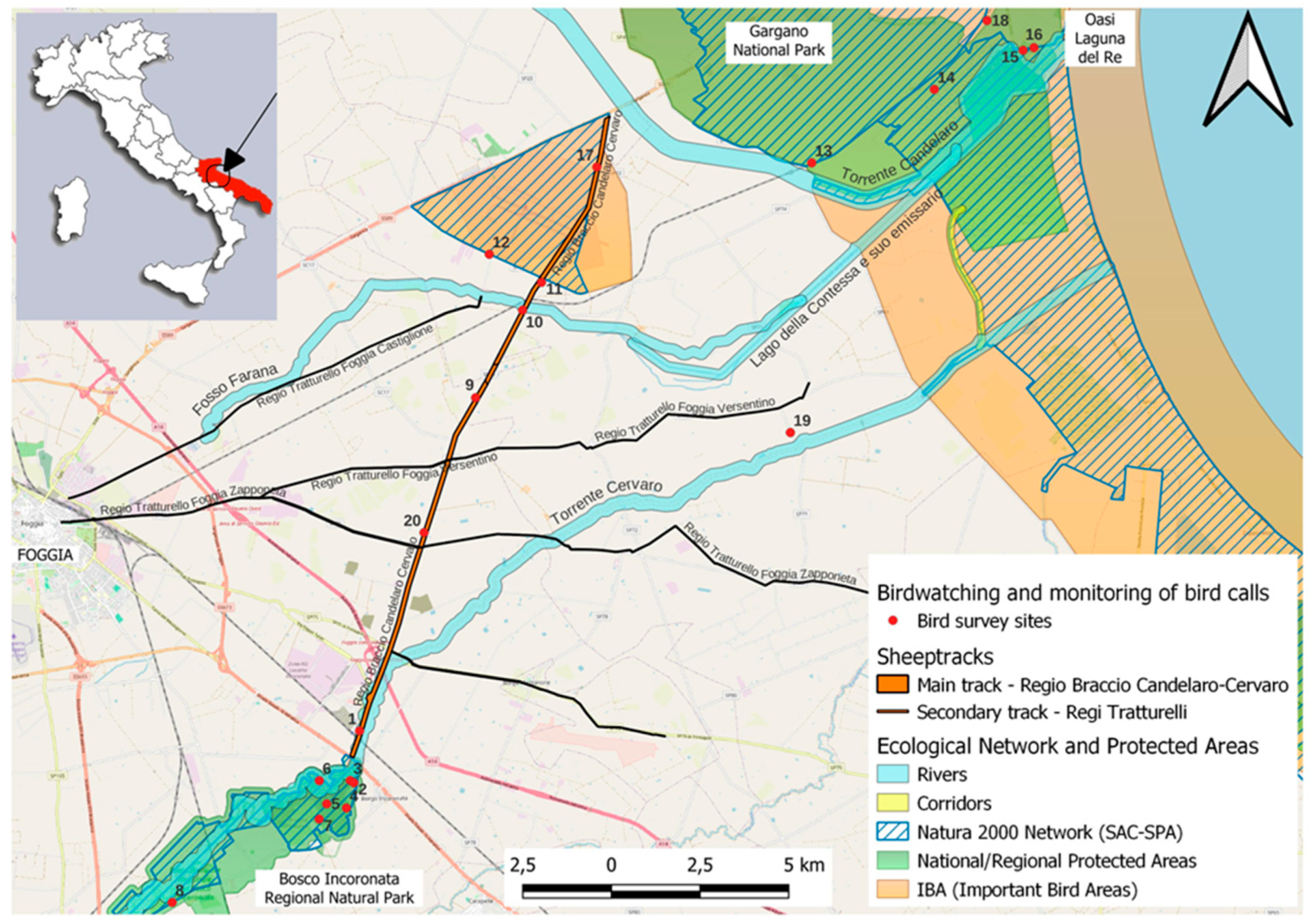
Figure 2.
Fuzzy membership functions of bird survey sites to the category of AGR, MIX and NAT according to the logistic equations, form Eq.1 to Eq.4 (reported in the text); MIX membership is represented by the red line (Eq.2 in the text), while AGR and NAT are represented by the green line (Eq.3 and Eq.4 in the text); the coefficients in Eq.1 are set as follows: G1=15% NAT or, alternatively, G2=65% NAT; K=0.35.
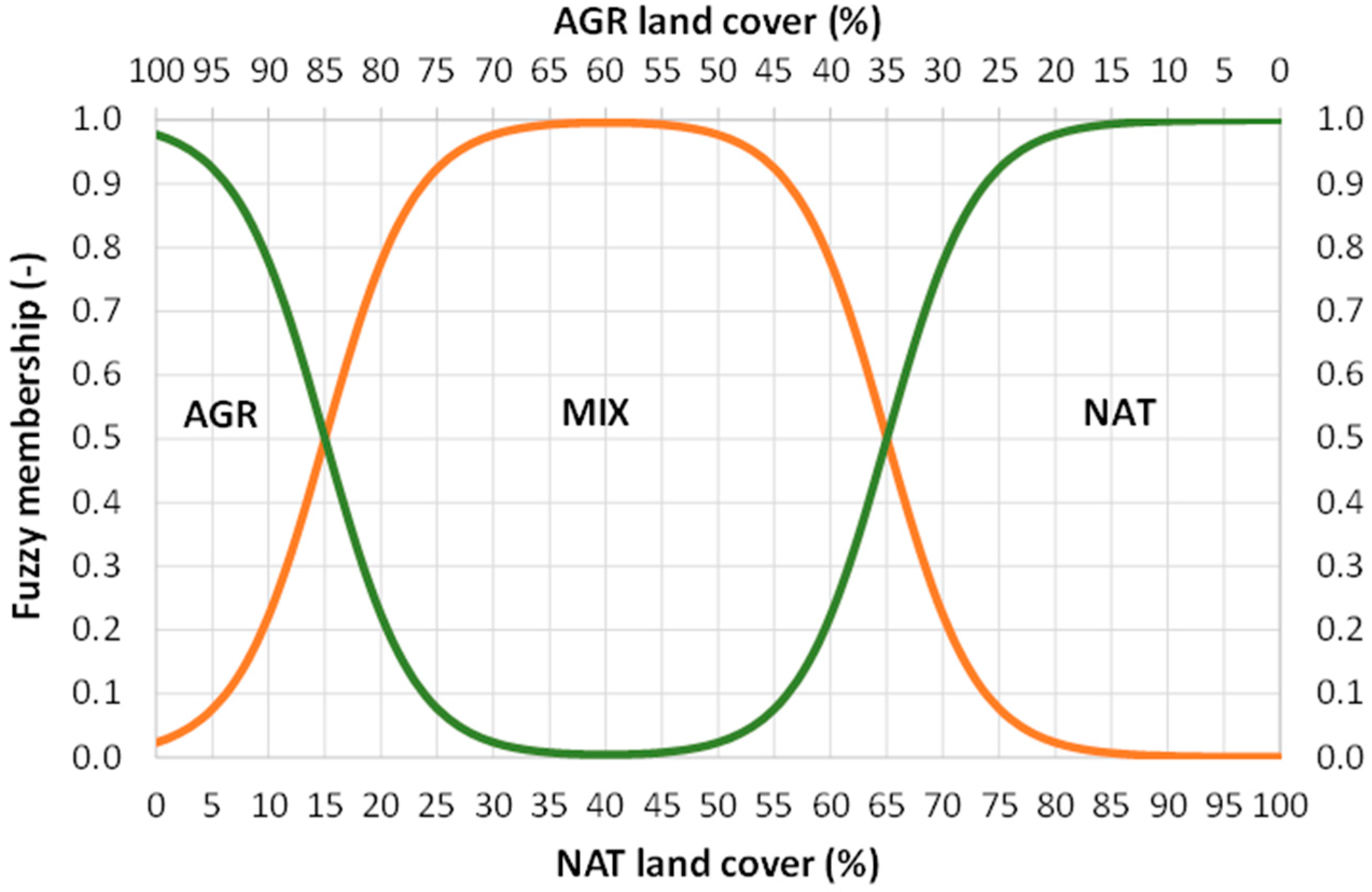
Figure 3.
Ecosystem category memberships of the 20 bird survey sites (indicated by their corresponding code number on the x-axis). Each bird survey site is defined by a fuzzy combination of AGR and MIX or, alternatively, of MIX and NAT partial memberships (their sum being equal to 1). The two horizontal dashed lines represent the assumed thresholds that crisply separate AGR from MIX (15%) and MIX from NAT (65%).
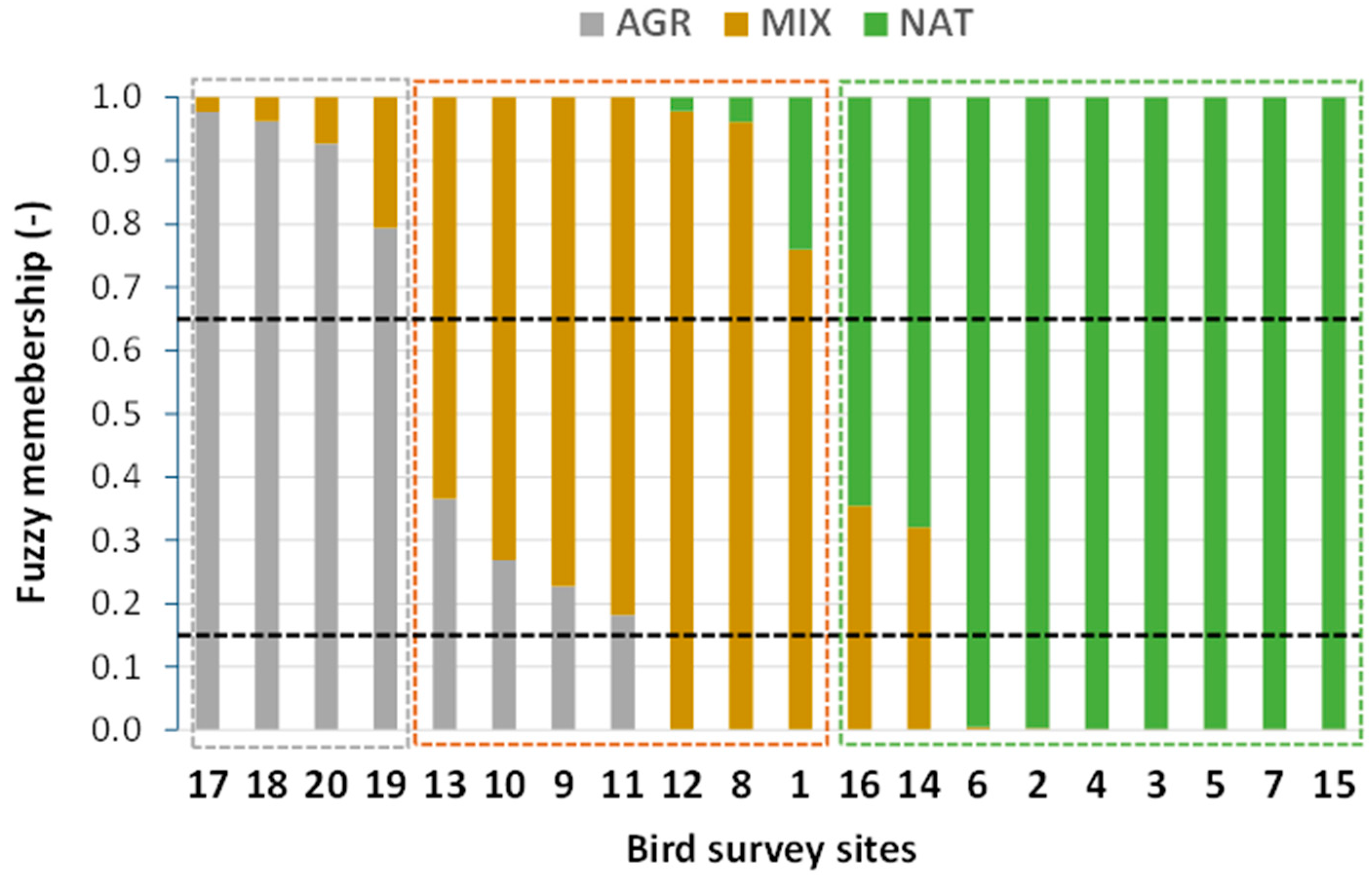
Figure 4.
Rank-abundance plots, also known as dominance-diversity curves or Whittaker plot. Bird species were assigned to ecosystem categories (AGR, MIX, and NAT) according to the partial membership corresponding to the survey sites where each species was detected. A smoothing spline function was used to regress the data (=0.05) and the confidence of the fit is also shown as a buffer to the regression line.
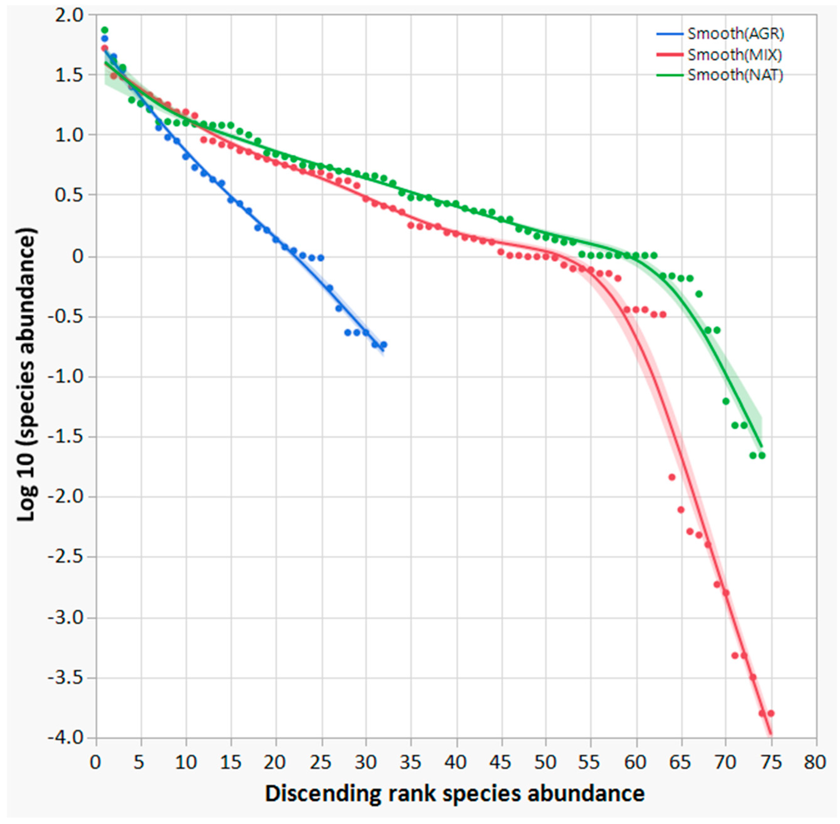
Figure 5.
Distribution of bird species in the three ecosystems categories AGR, MIX and NAT. The pie radius of each category is proportional to the total species richness. Different types of species relationships are shown: green sections indicate species common to all three categories, brown sections indicate species common to MIX and NAT, yellow sections indicate species common to AGR and MIX and finally orange sections indicate exclusive species, i.e. species found only in MIX or alternatively in NAT (as AGR has no exclusive species).
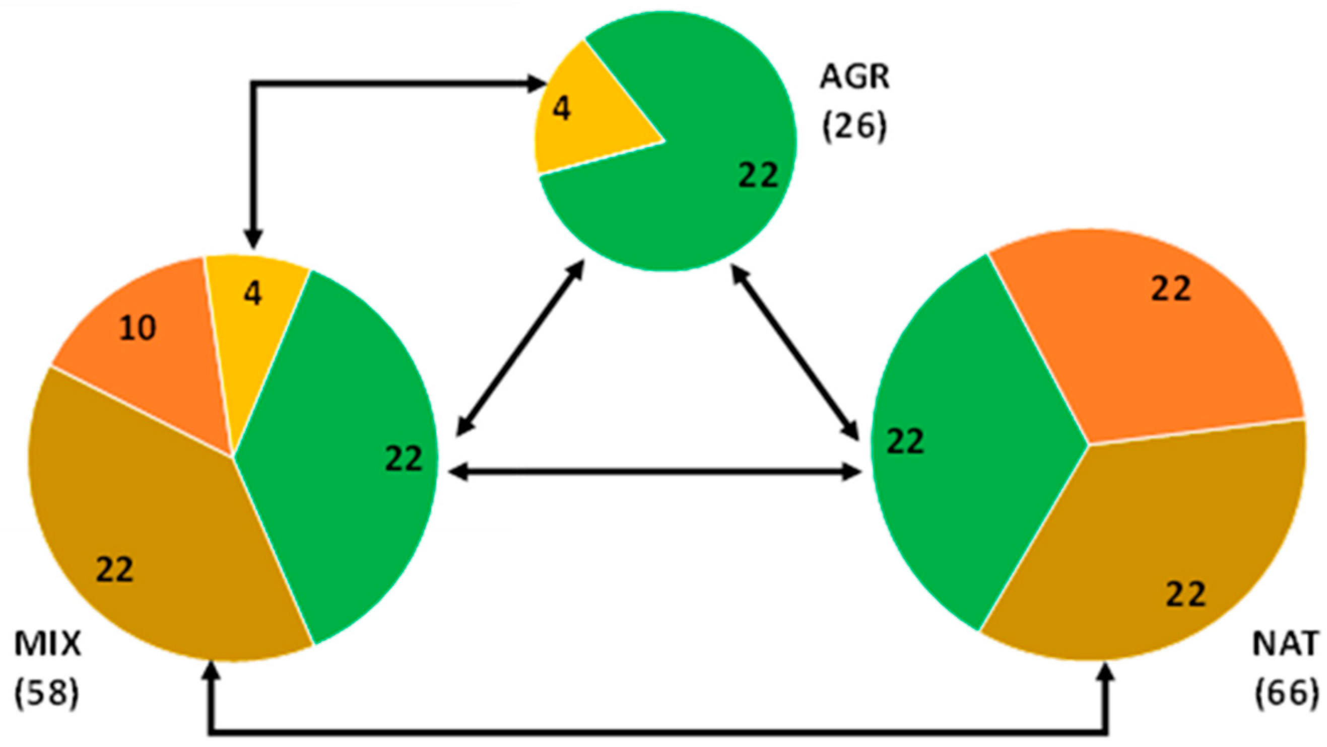
Figure 6.
Logistic probability curves discriminating the bird survey sites belonging to one of the three ecosystem categories (AGR, MIX and NAT) from the others. The lower curve in each graph (whose coefficients are statistically significant) concerns the discrimination of AGR from MIX; the upper curve in each graph (whose coefficients are not statistically significant) concerns the discrimination of MIX from NAT. The curve coefficients (intercept and slope) are reported in Table 4. The numbers in the plots refer to the identification code of the bird survey sites: the red ones are predominantly AGR, the blue ones predominantly MIX, and the green ones predominantly NAT, according to their fuzzy partial membership.
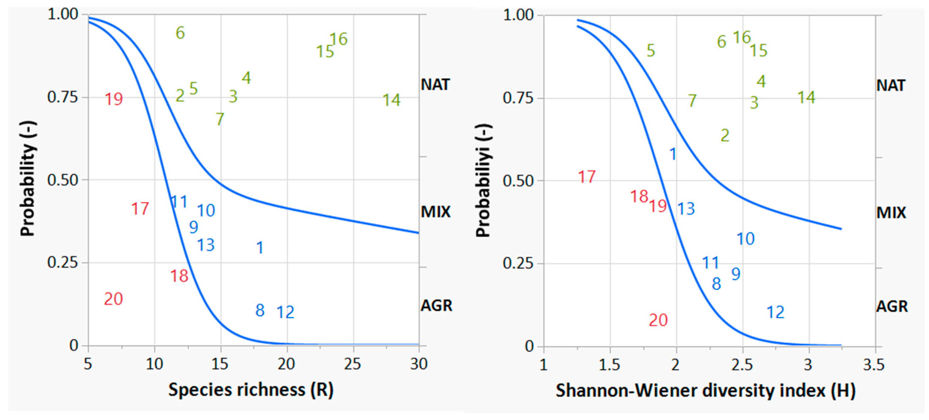
Figure 7.
Discriminant analysis of the bird survey sites according to their fuzzy membership to the three ecosystem categories (AGR, MIX and NAT). The biodiversity variables considered in the analysis are: Q - species abundance, R - species richness, H – Shannon Wiener biodiversity index and S - Simpson biodiversity index. The two canonical functions account for the total variability of the data (95.3% for the first and 5.7% for the second). The numbers in the plots refer to the identification code of the bird survey sites: the red ones are predominantly AGR, the blue ones predominantly MIX, and the green ones predominantly NAT, according to their fuzzy partial membership.
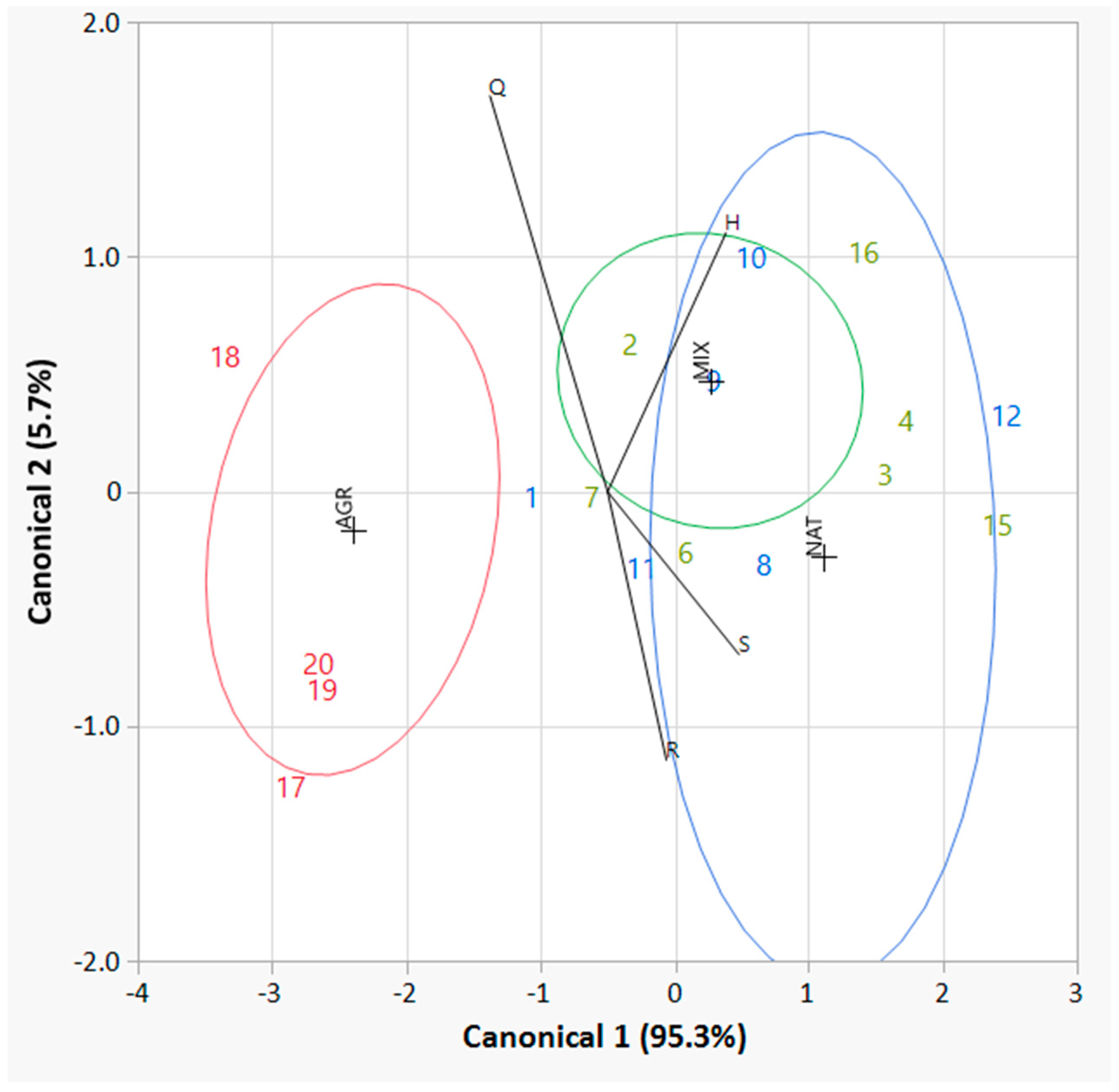
Table 1.
Classes of land use/land cover according to the EU Corine Land Cover (CLC) and the corresponding associated land macro classes applied in the present work. The areas of these land classes are also reported.
Table 1.
Classes of land use/land cover according to the EU Corine Land Cover (CLC) and the corresponding associated land macro classes applied in the present work. The areas of these land classes are also reported.
| Regional Land Use Map # | Present work | ||
| CLC classes | Description |
Land macro classes |
Area * (ha) |
| Utilized agricultural areas | Arable land, vineyards, olive groves, orchards, etc. | AGR | 29.5 |
| Wooded areas and semi-natural environments | Presence of forests, natural pasture areas, various types of vegetation, beaches, dunes and sands. | NAT | 26.4 |
| Wetlands | Wetlands, marshes, coastal lagoons | NAT | 5.5 |
| Water bodies | Rivers, streams, canals. | NAT | 1.4 |
# Reference: Regione Puglia, 2011 but updated by this work. * These areas are obtained by photo-interpretation and considering 20 bird survey points and a minimum radius of 100 m for each point (circular site area = π x r2; Total sampled area: 20 x 3.14 ha = 62.8 ha). Total AGR + Total NAT = 29.5 + 33.3 = 62.8 ha (Total sampled area).
Table 2.
Main compositional features of the bird communities in the three ecosystem categories (or ecosystems) AGR, MIX and NAT. Derived indices, as defined in the legend, are given as a footnote to the table.
Table 2.
Main compositional features of the bird communities in the three ecosystem categories (or ecosystems) AGR, MIX and NAT. Derived indices, as defined in the legend, are given as a footnote to the table.
| AGR | MIX | NAT | |
| 1. Species Abundance | 277 | 419 | 484 |
| 2. Species Richness | 26 | 58 | 66 |
| 2.a Exclusive species | 0 | 10 | 22 |
| 2.b Shared species | 26 | 48 | 44 |
| 3. Abundance / Richness | 10.65 | 7.22 | 7.33 |
| 4. Species Redundancy | 0.98 | 2.18 | 2.48 |
Legend: 1. Species Abundance = total bird detected; 2. Species Richness = species count; 3. Species Abundance/Species Richness (average N. of individuals per species); 4. Relative Species Richness is the ratio of Species Richness/Theoretical richness of equipartition, were the latter is equal to 80/3.
Table 3.
Results of the ANOVA and Duncan's post hoc test performed on Species abundance (Q), Species richness (R), Shannon-Wiener diversity index (H) and Simpson diversity index (S), considering land category membership values as weighting factor of the analysis.
Table 3.
Results of the ANOVA and Duncan's post hoc test performed on Species abundance (Q), Species richness (R), Shannon-Wiener diversity index (H) and Simpson diversity index (S), considering land category membership values as weighting factor of the analysis.
| Land | N. | Q(Sp. abundance) | R(Sp. richness) | H(Shannon-Wiener) | S(Simpson) | ||||
| Category | sites | Mean | Std Err. | Mean | Std Err. | Mean | Std Err. | Mean | Std Err. |
| AGR | 4.70 | 58.96 | ±11.74 | 9.87 | ±1.50 A | 1.83 | ±0.11 A | 0.549 | ±0.020 |
| MIX | 6.68 | 62.72 | ± 9.86 | 16.42 | ±1.26 B | 2.37 | ±0.09 B | 0.542 | ±0.017 |
| NAT | 8.62 | 56.14 | ± 8.68 | 17.16 | ±1.11 B | 2.41 | ±0.08 B | 0.558 | ±0.015 |
| 20.00 | p=0.88; n.s. | p=0.001; **. | p=0.0002; *** | p=0.77; n.s. | |||||
Different capital letters (A, B) indicate statistically significant differences between groups according to Duncan's post hoc test. For p values < 0.001, significance is denoted by ***; for p values < 0.01 then **; for p values < 0.05 then *; finally, for p values 0.05 then n.s. (not significant).
Table 4.
Results of nominal logistic regression applied to the values of our biodiversity indices: species abundance (Q), species richness (R), Shannon-Wiener diversity index (H) and Simpson diversity index (S), calculated in the 20 bird survey sites and assigned (using their membership values as weighting factors) to the three land categories (ecosystem categories AGR, MIX and NAT).
| Model term | Q | Std Err | R | Std Err | H | Std Err | S | Std Err | ||||
| AGR vs MIX | ||||||||||||
| intercept | -0.182 | ±1.157 | n.s. | 6.600 | ±4.28 | ** | 10.86 | ±6.50 | ** | 1.34 | ±5.37 | n.s |
| slope | -0.002 | ±0.016 | n.s. | -0.55 | ±0.34 | ** | -5.34 | ±3.12 | ** | -1.81 | ±9.78 | n.s. |
| MIX vs NAT | ||||||||||||
| intercept | -0.579 | 1.028 | n.s. | 0.27 | ±1.88 | n.s. | 0.72 | ±3.95 | n.s. | 2.25 | ±4.88 | n.s. |
| slope | 0.005 | 0.015 | n.s. | -0.03 | ±0.11 | n.s. | -0.41 | ±1.64 | n.s. | 4.55 | ±8.85 | n.s. |
| p=0.935 n.s. | p=0.007** | p=0.0145 * | p=0.869 n.s. | |||||||||
For p values < 0.01 then **; for p values < 0.05 then *; finally, for p values ≥ 0.05 then n.s. (not significant).
Disclaimer/Publisher’s Note: The statements, opinions and data contained in all publications are solely those of the individual author(s) and contributor(s) and not of MDPI and/or the editor(s). MDPI and/or the editor(s) disclaim responsibility for any injury to people or property resulting from any ideas, methods, instructions or products referred to in the content. |
© 2025 by the authors. Licensee MDPI, Basel, Switzerland. This article is an open access article distributed under the terms and conditions of the Creative Commons Attribution (CC BY) license (http://creativecommons.org/licenses/by/4.0/).
Copyright: This open access article is published under a Creative Commons CC BY 4.0 license, which permit the free download, distribution, and reuse, provided that the author and preprint are cited in any reuse.


