
Submitted:
13 February 2025
Posted:
14 February 2025
You are already at the latest version
Abstract
We use superoperator techniques to solve the master equation for the interaction between a quantized field and a moving mirror. The solution we provide allows its application to any initial state of the combined system. Furthermore, we obtain solutions to the stationary master equation for an initial number state for the field that is consistent with the result obtained for the average number of phonons.
Keywords:
Optomechanics
; Lindblad master equation
; superoperators
; quantum correlations.
1. Introduction
A cavity optomechanical system consists of an optical or microwave cavity with a movable mechanical component that can sustain collective vibrational modes [1,2,3]. A basic example of such a system is a cavity with two mirrors: one fixed and the other movable, which is coupled to a spring, allowing harmonic oscillations influenced by the radiation pressure of the field inside the cavity. This configuration enables a parametric modulation of the optical mode frequency of the cavity through the motion of the mirror.
Since the system cannot be completely isolated, there exists a coupling with its environment, introducing decoherence and dissipation effects such as photon leakage from the cavity and damping of the mechanical oscillator’s motion. On one hand, Mancini et al. [4] studied the case where the radiation mode loses energy much faster than the mechanical oscillator. By following an operator perturbation procedure, they managed to solve the system’s master equation. On the other hand, Bose and collaborators [5] solved the master equation for the optomechanical system considering the effect of damping on the mechanical oscillator’s amplitude by employing a technique that alternates between applying unitary and non-unitary evolution of the master equation over small time intervals, later taking the limit as time approaches zero. In [6], operator techniques are employed to transform the master equation of the optomechanical system, when subjected to environmental effects, into a master equation amenable to an analytical solution. In particular, they found that the optomechanical system with damping behaves as a free mechanical harmonic oscillator coupled to an environment, provided that the initial state of the cavity field is a thermal state.
The approach of superoperators for solving the master equation of a system has received little attention. The superoperator techniques involved in this approach consist, for instance, of defining superoperators that form a closed algebra under the commutation operation, allowing direct integration of the master equation and enabling the proposal of an ansatz to factorize the exponential of superoperators [7,8]. Alternatively, these superoperators can be used to apply transformations to the system’s density operator to rewrite the master equation into a form where its terms can be more easily manipulated, thus facilitating its analytical solution.
In this work, we employ superoperator techniques to solve the master equation in its Lindblad form for an optomechanical system subject to damping in the amplitude of the mechanical oscillator. Additionally, we compute and analyze the behavior of the average number of photons and, in particular, phonons in the damped optomechanical system, under the assumption that both the electromagnetic field and the mechanical oscillator are initially in coherent states. We also give a steady state solution for the master equation when the initial field state is given by a Fock state.
2. The Basic Optomechanical System
The system under consideration is a Fabry-Pérot cavity with one fixed end mirror and the other attached to a spring, allowing it to oscillate due to the radiation pressure force exerted by the cavity field, as shown in Figure 1. The Hamiltonian that describes this system, without damping, is given by [9] (we set )
where is the number operator of the cavity field, and are the position and momentum operators of the mechanical oscillator, with m and being its mass and natural frequency, respectively. The function represents the angular frequency of the cavity modes, given by [2,3]
where L and represent the length and the angular frequency of the cavity in the absence of interaction. We assume that the mirror displacement is small compared to the cavity length, i.e., . This setup enables the parametric modulation of the optical mode frequency of the cavity through the motion of the mirror. Since quantum harmonic oscillators are naturally described in terms of ladder operators, we use the relations and , where is the anhilation operator of the mechanical modes, to rewrite Equation (1) as
where is identified as the optomechanical coupling constant.
3. Optomechanical System with Damping in the Mechanical Oscillator
We consider an optomechanical system in which the movable mirror, modeled as a harmonic oscillator, is coupled to a zero-temperature environment, leading to the damping of the mechanical oscillator’s amplitude. The master equation describing the dynamics of the damped optomechanical system is given by (we set )
where is the density operator of the entire system and is the Hamiltonian from Eq. (3). The term is the Lindblad superoperator and is the damping constant of the mechanical oscillator.
Some authors [4,5,10] generally describe the dynamics of the optomechanical system by assuming that the Hamiltonian of the system is
that is, they neglect the contribution in the Hamiltonian (3). This approximation is valid as long as the number of photons is much greater than . However, as we will show, it is possible to perform a transformation to eliminate the linear term in the position of the mechanical oscillator in Equation (3), thereby obtaining the standard expression of the Hamiltonian.
3.1. Obtaining the Standard Hamiltonian in the Optomechanical Master Equation
As mentioned earlier, the Hamiltonian commonly used to describe the optomechanical system is the one given in Equation (5), however, we can recover that standard form of the Hamiltonian starting from the master equation in Equation (4), whose Hamiltonian is given by Eq. (3), by performing the following transformation:
where is the Glauber displacement operator [11]. Then, if , the master equation is transformed into
where , with . That is, we recover the same form of the Hamiltonian in Equation (5). Therefore, the master equation for the optomechanical system can be solved using the Hamiltonian given in Eq. (5).
3.2. Analytical Solution: Damping of the Mechanical Oscillator
In the rotating frame at the cavity field frequency, the master equation for the damped optomechanical system is given by
where , with denoting the frequency of the mechanical oscillator and the optomechanical coupling constant.
We can rewrite Equation (8) in the following form
where we have defined the following superoperators
The idea is to perform a series of transformations on the master equation that allow us to obtain equations with superoperators that are easier to handle. We transform Equation (9) with to obtain
where the superoperators and are defined as
Now, we perform the transformation , and with the appropriate choice of the parameter , we can eliminate the superoperator to obtain
with
A similar transformation may be performed to eliminate the superoperator, leaving only known terms that can be handled. Thus, we apply with to obtain
Now, we can directly integrate Equation (16), obtaining an exponential of the superoperators. Noting that
we find that the solution is
The next step is to express Equation (18) in factored form. To do so, let
as a result, we will have that
where we have explicitly expressed each superoperator and where we identify
Therefore, we find that the solution to Equation (20) is
We observe that the set of operators in the exponentials is individually closed under commutation [12]. Consequently, we can write it as a product of exponentials by applying the Wei-Norman theorem [13]. It is found that
and
with
Since we have already factored the exponentials, we can now return to the original frame by applying the inverse transformations, that is, using the fact that
Finally, the solution to the master equation (8) will be given by
3.3. Coherent States as Initial Conditions
Considering that initially both the cavity field and the mechanical oscillator are in coherent states and , respectively, then, the density operator that describe the initial state of the system is given by . In this way, it is found that
Considering that , , then , so it will follow that
In order to calculate the result of applying and to , we note the following: By expressing the coherent state of the field in terms of its corresponding Fock states, we find that
where are the number states of the field, are the coherent states of the mirror,
and
Then, given that , we obtain that
By applying the corresponding superoperators, it is found that the density operator of the composite system is given by
Using the explicit form for the functions and with we obtain the average number of photons
and the average number of phonons
where
and
We observe that the average photon number in the cavity remains unchanged, as expected, given that only the mirror’s damping is considered. Meanwhile, the average number of phonons depends on both the mean photon number in the cavity and its square, . In general, we observe a damped oscillatory behavior due to the appearance of decaying exponentials, , multiplied by periodic functions. In the limit , we have that
that is, the average phonon number, in general, does not tend to zero.
In Figure 2, the time evolution of the phonon number of the mechanical oscillator is shown when the initial state of the mirror is a coherent state with , for different values of the coherent state amplitude of the field , where , , and .
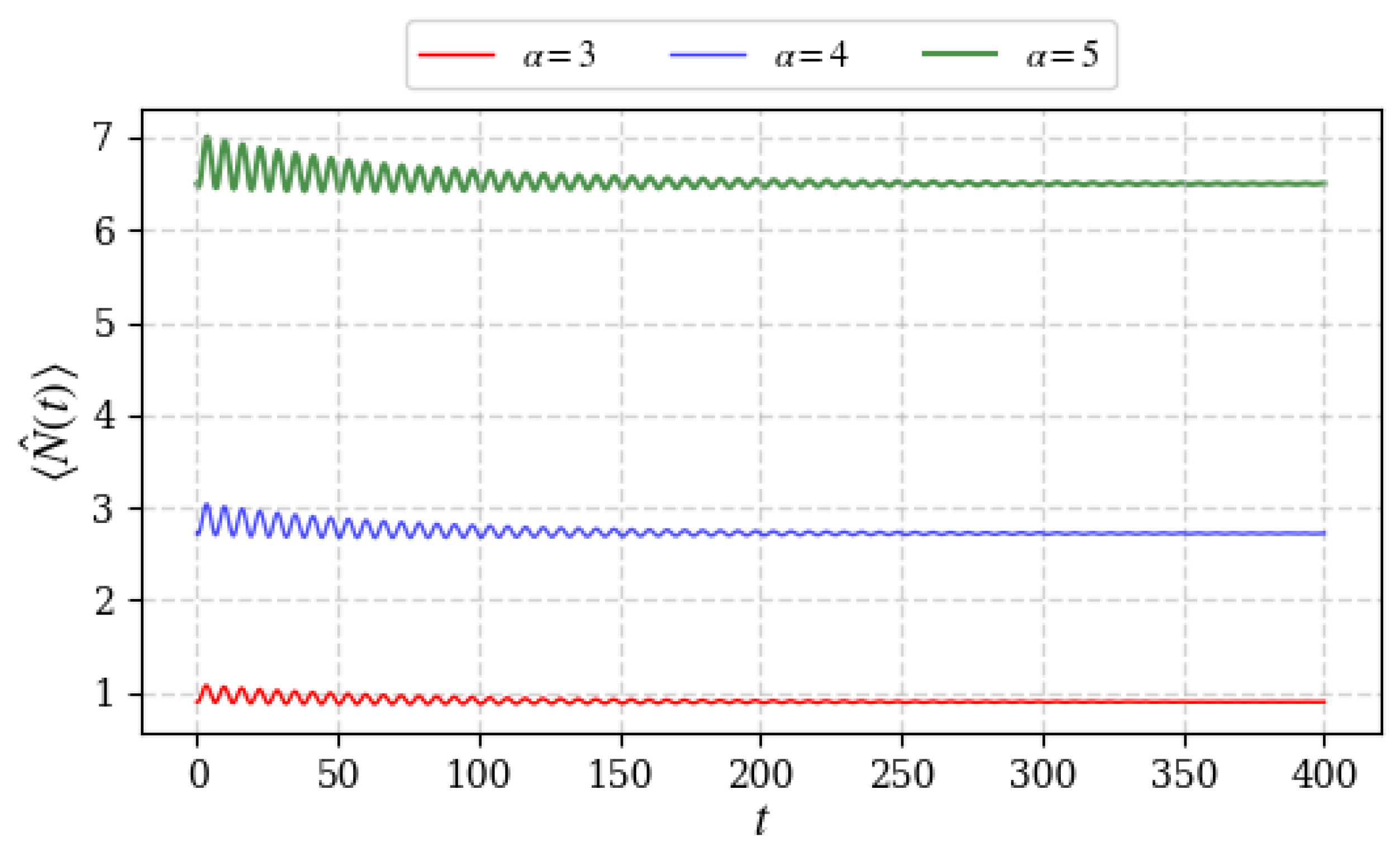
Figure 3, illustrates the specific case in which the initial state of the mechanical oscillator is given by the square root of the phonon number from Equation (41). As a consequence, in the limit , the system recovers the initial phonon number. That is, even though the mechanical oscillator is coupled to the environment, the initial phonon number can be recovered under appropriate initial conditions. This behavior is shown for different values of the coherent state amplitude of the field , with parameters , , and .
It is worth noting that for a lossless optomechanical system, , we obtain the same results reported in [12] for the average phonon number
3.4. Steady State
A steady-state solution to equation (8) may be obtained by assuming that the cavity field is in the Fock state , while the mechanical oscillator occupies a state , to be determined under the condition . Consequently, the system’s density operator is given by
where, by substituting (43) into the master equation (8), we obtain
To solve this equation, we apply the following transformation
where, by choosing , we obtain an equation in which the term is eliminated, yielding
and this equation is satisfied if . Therefore, in the original frame, it is found that the density operator that makes the system stationary is
where is a coherent state. Furthermore, we note that the average number of phonons is
which is consistent with Equation (41).
4. Conclusions
We have given a superoperator solution to the master equation that describes the interaction between a quantized field and a moving mirror. Unlike the solution given by Bose et al. [5], our solution allows any initial wavefunction of the combined system. We also presented a steady state solution of the master equation that gives consistent results with the average number of phonons at .
References
- Aspelmeyer, M., Meystre, P., & Schwab, K. (2012). Quantum optomechanics. Physics Today, 65(7), 29-35.
- Meystre, P. (2013). A short walk through quantum optomechanics. Annalen der Physik, 525(3), 215-233. [CrossRef]
- Bowen, W. P., & Milburn, G. J. (2015). Quantum optomechanics. CRC press.
- Mancini, S., Man’Ko, V. I., & Tombesi, P. (1997). Ponderomotive control of quantum macroscopic coherence. Physical Review A, 55(4), 3042. [CrossRef]
- Bose, S., Jacobs, K., & Knight, P. L. (1997). Preparation of nonclassical states in cavities with a moving mirror. Physical Review A, 56(5), 4175. [CrossRef]
- Ventura-Velázquez, C., Rodríguez-Lara, B. M., & Moya-Cessa, H. M. (2015). Operator approach to quantum optomechanics. Physica Scripta, 90(6), 068010. [CrossRef]
- Arévalo-Aguilar, L. M., & Moya-Cessa, H. M. (1995). Cavidad con pérdidas: una descripción usando superoperadores. Revista Mexicana de Física, 42(4), 675-683.
- Moya-Cessa, H. (2006). Decoherence in atom–field interactions: A treatment using superoperator techniques. Physics reports, 432(1), 1-41. [CrossRef]
- Law, C. K. (1995). Interaction between a moving mirror and radiation pressure: A Hamiltonian formulation. Physical Review A, 51(3), 2537. [CrossRef]
- Mancini, S., & Tombesi, P. (1994). Quantum noise reduction by radiation pressure. Physical Review A, 49(5), 4055. [CrossRef]
- Glauber, R. J. (1963). Coherent and incoherent states of the radiation field. Physical Review, 131(6), 2766. [CrossRef]
- Medina-Dozal, L., Récamier, J., Moya-Cessa, H. M., Soto-Eguibar, F., Román-Ancheyta, R., Ramos-Prieto, I., & Urzúa, A. R. (2023). Temporal evolution of a driven optomechanical system in the strong coupling regime. Physica Scripta, 99(1), 015114. [CrossRef]
- Wei, J., & Norman, E. (1964). On global representations of the solutions of linear differential equations as a product of exponentials. Proceedings of the American Mathematical Society, 15(2), 327-334.
Figure 1.
Diagram of an optomechanical cavity system. A Fabry-Pérot cavity with a length L contains an optical mode with frequency and the annihilation operator for the electromagnetic modes is . One of the cavity mirrors is mounted on a mechanical oscillator with frequency and the annihilation operator for the mechanical modes is . The optomechanical interaction arises due to the radiation pressure exerted by the optical field on the movable mirror, where represents the displacement of the mechanical oscillator. The mechanical dissipation is characterized by the damping rate .
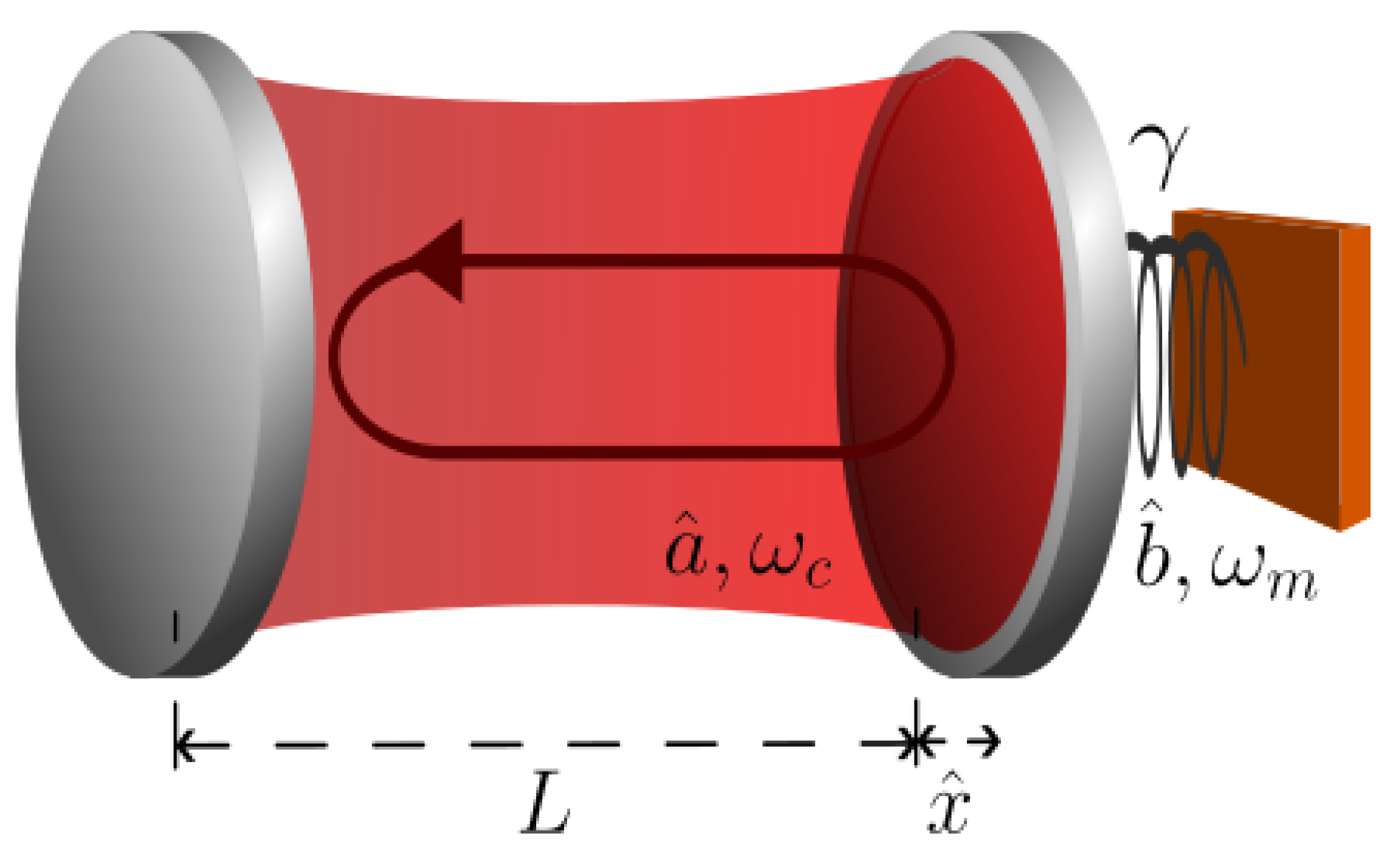
Figure 2.
Temporal evolution of the average phonon number with an initial amplitude of the coherent state of the mirror with parameters for different values of the amplitude of the coherent state of the field .
Figure 2.
Temporal evolution of the average phonon number with an initial amplitude of the coherent state of the mirror with parameters for different values of the amplitude of the coherent state of the field .
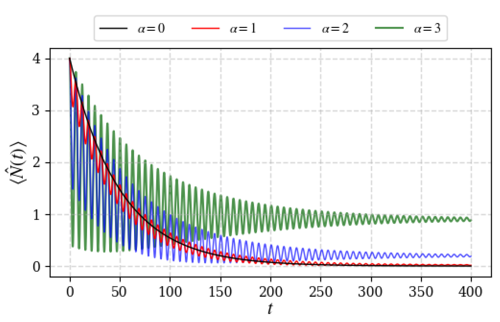
Figure 3.
Temporal evolution of the average phonon number when the initial state of the mechanical oscillator is given by the square root of the phonon number in equation (41) for different values of the amplitude of the coherent state of the field , with parameters .
Figure 3.
Temporal evolution of the average phonon number when the initial state of the mechanical oscillator is given by the square root of the phonon number in equation (41) for different values of the amplitude of the coherent state of the field , with parameters .
Disclaimer/Publisher’s Note: The statements, opinions and data contained in all publications are solely those of the individual author(s) and contributor(s) and not of MDPI and/or the editor(s). MDPI and/or the editor(s) disclaim responsibility for any injury to people or property resulting from any ideas, methods, instructions or products referred to in the content. |
© 2025 by the authors. Licensee MDPI, Basel, Switzerland. This article is an open access article distributed under the terms and conditions of the Creative Commons Attribution (CC BY) license (http://creativecommons.org/licenses/by/4.0/).
Copyright: This open access article is published under a Creative Commons CC BY 4.0 license, which permit the free download, distribution, and reuse, provided that the author and preprint are cited in any reuse.


