
Submitted:
03 April 2025
Posted:
04 April 2025
You are already at the latest version
Abstract
The transition of the chemical industry towards the utilization of feedstocks based on renewable energies results in a more dynamic process behavior. Advanced mathematical methods are a key factor to handle this complexity. In this contribution, methanol synthesis from hydrogen, carbon dioxide and carbon monoxide is investigated as promising power-2-X technology. Optimal experimental design is used to recalibrate an existing mechanistic kinetic model. Subsequently, the most uncertain sub-model, namely the reversible catalyst dynamics, is partially replaced by neural networks. Several architectures were evaluated, and optimal experimental design was applied to enhance the performance of a chosen architecture. All experiments were realized in an experimental setup able to acquire time-resolved data. A commercial CuO/ZnO/Al2O3 catalyst was used in a well-mixed Berty type reactor. The combination of optimal experimental design with hybrid modeling led to an improved quality of the kinetic model needed for process control and optimization.
Keywords:
methanol synthesis
; optimal experimental design
; data-driven modeling
; optimal control
; scientific machine learning
1. Introduction
Methanol is an essential chemical with various applications. Next to its use as an intermediary product in synthesizing complex chemicals, it can be used to store electrical excess energy from renewable sources ([1]). As such, power-2-methanol processes are practical options for both synthesizing methanol from and storing said energies. Typically, green hydrogen produced via the electrolysis of water using electrical energy from renewable resources serves as the basis for this process. Hence, it is subject to inherent fluctuation of the energy source and, in turn, to comparable highly dynamic operating conditions. Advanced control schemes are needed to maximize the throughput of the process and allow the maximization of the process conversion rate under these non-stationary environmental conditions. Model-based (optimal) control is often at the heart of such strategies, see e.g. [2]. Although methanol synthesis is an established process, the development and research on the mechanism has been and still is an active field of research ([3,4]). To this end, hybrid models often serve as a valid alternative to classical, entirely mechanistic approaches. Here, machine learning models, such as neural networks, replace partially unknown or uncertain parts to account for the lack of prior scientific knowledge. Especially in the context of (industrial) chemical process engineering, training these models poses a non-trivial issue: How can hybrid models be trained reliably with minimum amount of data? This work shows how optimal experimental design can help to improve parameter estimation in the physics based model for the reaction kinetics developed by [5,6,7], which will act as a baseline for our evaluation, and fitting of hybrid models. The model quantifies the heterogeneously catalyzed synthesis of methanol using hydrogenation of CO and CO2 over a CuO/ZnO/Al2O3 catalyst. The underlying reaction network is shown in Figure 1 and hints at the complexity of the chemistry. The overall reaction can be broken down to three main equilibrium-limited reactions: the hydrogenation of carbon monoxide (Equation 1), the hydrogenation of carbon dioxide (Equation 2) and the reverse water-gas shift reaction (Equation 3).
To mathematically describe the chemical relationship, we start from the mechanistic model derived and parameterized in [5,6,7] with experimental data acquired by [8]. In earlier work the deactivation of the catalyst was not taken into account for the parameter identification, but will be considered within this contribution. Due to that reason and additional aging effects of the catalyst stored over several years, the mechanistic model was recalibrated first in this project. Subsequently, optimal experiments were designed and realized to improve the mechanistic model further.
Next, we move on replacing a part of the differential algebraic equation model with a neural network, following [9], which was trained on experimental data generated thus far. Using the approaches proposed in [10], we compute an additional experimental design aimed at generating further insightful data for the training of this hybrid model.
The rest of the paper is structured as follows: In Section 2, we introduce the used methods and materials. We start by describing a newly built experimental set-up containing a well-mixed Berty type reactor as the data-generating unit. In the following, we introduce the mechanistic model, motivate the use of its hybrid counterpart, and provide a brief introduction to optimal experimental design from the perspective of optimal control. Section 3 evaluates the results of the derived models, focusing on the difference in predictive performance when including or excluding optimal experimental design. Section 4 concludes this paper by discussing the results and outlining further research directions. Our contribution focuses on new insights in:
- new experimental dynamic and steady state data for methanol synthesis considering the changes of catalyst activity
- comparison of mechanistic and hybrid model, by replacing a subset of the heuristic model with a neural network
- conducting and evaluating OEDs for a mechanistic and a hybrid model, examining the impact on different hybrid model strategies.
2. Materials and Methods
2.1. Experimental Set-Up
Experimental data is acquired in a self developed automatic set-up depicted in Figure 2. The reaction is carried out in a gradient-less Berty-type reactor built by the FAU Erlangen Nuremberg according to [11]. It contains a fixed bed of 4.3 g commercial CuO/ZnO/Al2O3 catalyst (CZA) from BASF which had been ground to 0.315-0.5 mm particles to avoid intraparticular transport limitations. The used catalyst was acquired in a former PhD project ([8]) and was stored at ambient conditions since then. The remaining gas volume of the reactor is approximately 280 mL including inert filling material as spherical -Al2O3 (charge no. 5) or 286 mL without additional filling (charge no. 6). To verify the assumption of an ideal CSTR behavior, the rotation speed of the stirrer had been varied during preliminary tests. Above 3000 rpm no changes were observed. Giving additional safety, we choose to set the rotation speed to 4000 rpm. The stirrer is driven by an electric engine, equipped with permanent magnets that disintegrate when interacting with hydrogen or hydrocarbons. Due to constructional reasons, the engine is connected to the reaction chamber. Furthermore, permanent magnets lose their field strength when heated, so the stirrer performance would be permanently negatively affected. For these reasons, it is particular important to cool and flush the engine of the stirrer with nitrogen. This constrains the concentration of the educts. Since, nitrogen is an inert for the reaction, it is used as an indicator for the occurring volume contraction. The experimental set-up is designed for reaction conditions up to 260 °C and 60 bar.
The utilized gases are supplied from gas bottles with a high purity of 99.999 vol.-% for N2, H2 and CO2 and 99.97 vol.-% for CO. Bronkhorst mass flow controllers (MFC) are used to dose the educt gases (further information in Appendix A.2). Additional piping length is given to mix the gases at the inlet and precondition them for the reaction. In order to prevent condensation, the entire piping periphery around the reactor is heated.
The experimental set-up is designed to perform steady state and dynamic experiments under isothermal and isobaric conditions. Changes in temperature and pressure during operation are recorded and can be evaluated posterior. However, due to the sheer caloric mass of the reactor, intentional alterations in temperature within an experiment are unfavorable. They greatly increase the required time for an experimental investigation. Therefore experiments are mostly designed to remain at a certain temperature.
Several temperature probes are located in and around the reactor. One sensor is situated above and one beneath the catalyst bed. Two further sensors are measuring the heating jacket. Since only a small amount of enthalpy is released from the reaction and the great thermal mass of the reactor itself is acting as a dampener, one of the jacket sensors is used to control the reactor temperature. This has proven to be the most stable operation to maintain a constant reaction temperature.
A dome pressure regulator (Equilibar) was used to control for constant pressure in the reactor allowing a discharge during continuous experiments. As analytic devices are usually particularly sensitive regarding their inlet pressure, the outlet stream after the dome pressure regulator is first depressurized via a relief valve to 4 bar and afterwards further reduced to 1 bar using a Swagelok downstream pressure regulator. This method ensures constant pressure at the analytics while inlet conditions to the reactor can be dynamically modified. The total volumetric flow rate at the reactor outlet is not measured. If the reactor pressure is increased during an experiment the dome pressure regulator reduces the outlet flow until the pressure level is reached. In this case the flow rate to the analytics could be inappropriate.
One part of the automation is managed by Siemens’ PCS7, acquiring plant related data and operating all actors. The other part of automation is realized via MATLAB in the interest of applying complex mathematical inlet perturbations, precise timing of new conditions, creating a flexible, user friendly interface and recording data during the time of an experiment for simpler analysis. PCS7 and MATLAB where connected through Open Platform Communication Data Access (OPC DA), a proven industrial communication standard.
This allows imposing classical step changes between different constant input values with varying time intervals, as well as periodical perturbation of inlet conditions (e.g. simultaneous modulation of inlet concentration and total flow rate as phase shifted sinusoidal wave form) as shown in Figure 3, making this plant an unique experimental set-up. Besides that, another degree of freedom is the use of different fillings of the reactor with fresh catalyst. We refer to this by a catalyst "charge number".
Outlet concentrations are quantified in terms of molar fractions of the components CH3OH, CO2, CO, H2, H2O and N2 using a µ-GC from Agilent (model 490). Samples are measured by a method that takes approximately 90 s, which had been optimized to execute with precise component determination and fast sampling. This enables an almost continuous collection of data points. Further details about the analytics are summarized in Appendix A.1.
2.2. Experimental Procedure
When fresh catalyst was filled into the reactor, it was reduced using 2 vol.-% of H2 in N2 with a total volumetric flow rate of 500 NmL/min at ambient pressure starting from room temperature heating up to 180 °C within 2 h and holding the temperature for another 12 h according to [8]. This procedure was repeated after every plant shutdown and sometimes additionally to check for the effect on the catalytic performance. Otherwise the catalyst was flushed with nitrogen between methanol synthesis experiments.
To start a methanol synthesis experiment with already preconditioned catalyst the flow of the inert flushing of the stirrer is increased depending on the aimed pressure and the stirrer speed is set to 4000 rpm. Afterwards, the inertized reactor is heated up at ambient pressure to the desired temperature. Meanwhile the pressure of the gas supply is adjusted. While N2, H2 and CO are fed directly from gas bottles, CO2 is pressurized with a compressor from Maximator to reach up to 65 bar. The CO2 piping is heated to avoid condensation. After the temperature is reached, the pressure is built up with the dome pressure regulator feeding only N2. At the same time, the heating of the entire piping periphery, the analytics, the process control system and the data acquisition must be prepared. Then an experiment can be started by dosing the reactants with the MFC. When the experiment is finished, the reactor is depressurized, inertized and most of the time cooled down to 180 °C.
Catalysts are known to deactivate during operation ([12]). The deactivation of the CZA methanol synthesis catalyst is addressed in several studies, e.g., [13,14,15]. Catalyst deactivation is not the focus of this contribution, but must be taken into account. To quantify irreversible deactivation effects, a daily updated catalyst activity was measured prior to a new experimental run. This is done by applying a reference condition summarized in Table A1. The condition is maintained until steady state is reached. Applying this procedure, a deactivation independent evaluation of the generated kinetic data is attempted. Additionally, due to the initial exposure to the same feed and thus the same reduction potential the catalyst is preconditioned with regard to reversible dynamic changes of the active sites. After that, the desired experiments were started.
The hydrogenation reactions (namely reaction Equation 1 and Equation 2) cause a reduction in the total number of moles and thereby induce a volume contraction, which we define as the ratio of inlet to outlet molar fraction of the inert nitrogen. Multiplying this ratio to the inlet volumetric flow rate under norm conditions (273.15 K and 1.01325 bar, indicated in the superscript as "n" and all flow rate values given in this paper are refering to this condition) results in the norm outlet flow rate :
Given the experimentally recorded molar fractions of each component i, the above calculated total outlet volumetric flow rate and the ideal gas law concludes to the corresponding outlet molar flow rate :
Engineering metrics as the carbon based yield of methanol can be calculated as shown in Equation 6. This value results from the ratio of calculated outlet molar flow rate of methanol to the sum of input molar flow rates of all carbon species (i.e. CO and CO2).
The value of the catalytic activity a is determined via calculating the current methanol yield with Equation 6 divided by the initial methanol yield determined with the fresh catalyst of the corresponding charge, i.e. the stationary outlet result under reference condition after 1st reduction (Equation 7).
The catalytic activity a is used as an identical pre-factor for all three reaction rates as shown in Equation 8.
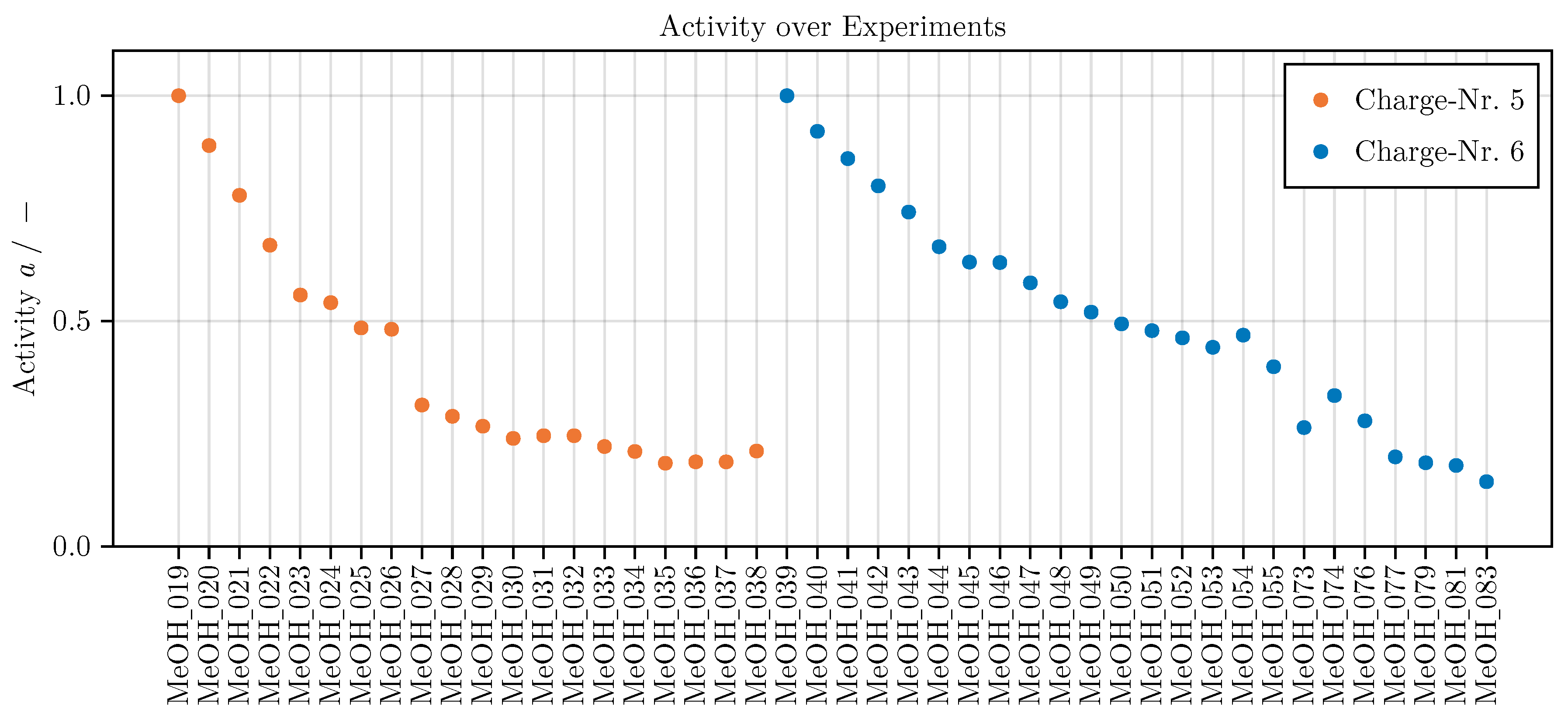
We assume that the deactivation influences all three reactions Equations (1)–(3) in the same way and does not change drastically over the course of one specific experiment. Thus, a is one fixed value for every experiment, ranging from 0.14 to 1 for the entire data used in this work and from 0.14 to 0.33 for the optimally designed experiments. This allows the evaluation of our data without being distorted by deactivation effects.
The complete set of experimental data used in this contribution is available under [?].
2.3. Mechanistic and Hybrid Modeling of the Methanol Synthesis
We base our approach upon the established kinetic model, capable to quantify the rates of the three key reactions proceeding during methanol synthesis, derived in [5,6,7] (see Section Appendix B). This kinetic model is connected to the mass balances valid for an ideally mixed, isothermal, isobaric and continuously operated reactor model. The whole model consists of a set of differential-algebraic equations (DAE) of the form
Here denotes the time and denotes the state which consists of the mole fractions of the six chemical species , CO, , , , and an additional state which represents the distribution of the active centers of the catalyst. The operator ⊙ denotes elementwise multiplication, denotes a set of parameters (see Section Appendix C.1) and the inputs of the system, which consist of temperature, pressure, feed and flow. The matrix valued functions account for the gradient of the surface coverage of the individual species and combines the stoichiometric coefficients with the catalyst mass (constant for every experiment) in dependence of the states. denotes the activity level of the catalyst as described in Section 2.2.
An important feature of the kinetic model is the incorporation of dynamic changes of the catalyst. captures the influence of the degree of reduction of the catalyst on each of the reaction rates. Of special interest are the three scaling pre-factors , which were previously modeled based on a heuristic
which only depends on the catalyst state ([5,6]). In this work, we propose to replace this heuristic with a fully connected feed-forward neural network to describe , resulting in a hybrid model. Hybrid modeling aims at combining the advantages of two different modeling paradigms. First, the interpretability and data-efficiency of rigorous modeling based on first principles and specific domain knowledge, and second the flexibility of data-driven models such as neural networks, which are able to learn unknown functional relationships from data. In recent research various modeling regimes and architectures have been investigated, see e.g. [16] or [17] for an extensive overview. In the context of differential equations, such models are commonly called universal differential equations ([9]).
The hybrid DAE model can be written in its implicit form as
where describes the parts of the model which are known from first principles and which may depend on physical parameters . Second, a universal approximator, e.g., a feed-forward neural network, with weights and biases is used to model the unknown parts of the dynamics. The function encodes the overall structure of the hybrid model, i.e., how known and unknown parts of the dynamics interact. Figure 4 shows the mechanistic model in the form of a block diagram, highlighting the catalyst impact which we are replacing.
2.4. Data Preparation
The collected experimental data was divided into a training and test data set using a stratified 80-20 train-test split, see Section Appendix C.3. Here denotes the set of state measurements of the reactor output and the set of inputs consisting of feed composition, flow rate, pressure and temperature. Finally, denote the time points of the measurements.
2.5. Parameter Estimation
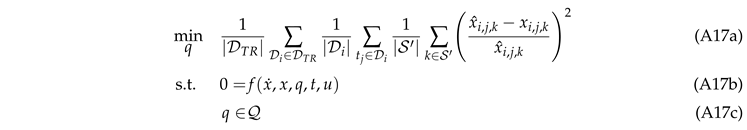
The parameter estimation was performed by solving the following optimization problem:
We used an average sample-wise Equation 12a between the measurements (outlet molar fractions) and predictions x given by the weighted sum-of-squares error
We included only a subset of species, namely the carbon-based species with a high accuracy in the analytics and water as co-product, present often only in small amounts but very important for the kinetic model. The weights have been chosen to be , , to adjust the contribution of each species relative to its magnitude. 12b describes the dynamics of the system. Instead of modeling the domain 12c, we used the exponential transformation to ensure that a subset of parameters is positive to account for its physical meaning. The initial conditions and domains of the parameters have been set according to [7], and can be seen in Section Appendix C.1. We implemented our model and optimization1 in Julia ([19]). To solve Equation 12, we used Optimization.jl ([20]), a solver agnostic interface to several optimization routines. To fit the mechanistic model, we used the implementation of L-BFGS ([21]) of Optim.jl ([22]). To investigate the impact of the experimental designs, once the parameter estimation problem is solved on the full training data with all experimental designs and once on the training data excluding the optimal experimental designs.
2.6. Hybrid Model Fitting
To find a suitable candidate for the hybrid model, we performed a simple hyperparameter search over different architectures by employing a full factorial design over the number and size of the hidden layers as well as their activation function in Lux.jl ([?]). We adapted Equation 12 by adding a L1 norm regularization with regularization parameter on the weights of the network to counteract overfitting. The options of this hyperparameter search are given in Table 1. The neural networks are modeled to take the full state x as an input. Moreover, the output layer uses the softplus function , to ensure a positive output. Each candidate architecture has been trained five times with different random seeds used for initialization of the weights for a total number of 500 iterations using Adam ([23]) from Optimisers.jl and mini-batching of the data set. Next, a suitable candidate has been selected by accounting for both complexity of the network and conformity with the data. We selected the top-k candidates using the coefficient of determination on the training set and subsequently retrained these models using L-BFGS.
2.7. Optimal Experimental Design
To minimize the effort of experimental data collection, we want to collect as much information about the uncertain parameters as possible from each experimental run. Optimal experimental design (OED) is a well-established concept in Chemical Engineering ([24,25]) and a natural approach to come up with informative experiments for subsequent parameter estimation problems or model identification. See [26,27,28,29] for a general introduction into the topic. In [30,31] the concept was applied to dynamical systems given by parameterized ODE or DAE models. In this context, degrees of freedom are the decisions when to measure each observed variable and how to stimulate the system in an optimal way. The problem of computing an optimal experimental design can thus be cast as an optimal control (OC) problem, see Appendix E.1 for detailed explanation. The goal is to optimize the time-dependent inputs and the initial conditions such that a suitable objective function of the variance-covariance matrix is minimized. This requires to augment the system using the forward sensitivity equations and the differential equation of the Fisher information matrix, adding states in the order of .
In this work, we use OED in two ways. First, we use it to compute four informative experiments for estimating the physical parameters of the heuristic model. More specifically, these experiments each aim at the identification of different subsets of parameters, namely the parameters in the Arrhenius equations of the three elementary reactions and two rate constants in the kinetic equation for the state . Second, in the case of a hybrid model, i.e., the parameters q of the underlying model include both physical parameters and weights and biases of a neural network . In this context, the OED problem may also be solved aimed at generating data to train the embedded neural network on. However, problems may arise due to the usually large parameter space of the neural network. The quadratic dependence of the size of the augmented system of differential equations on the number of parameters as explained above leads to a high computational effort even for integration of the augmented system. Moreover, setting up the variational differential equations analytically may be prohibitively expensive. Another difficulty arises from the observation that weights of neural networks are not uniquely identifiable. Therefore, resulting Fisher information matrices in the underlying optimization problem are usually ill-conditioned and not amenable to optimization. However, as argued in [10], one can often circumvent these problems by identifying a suitable subset of parameters via a singular value decomposition of the Fisher information matrix. This way, the size of the system of differential equations is reduced and positive definiteness of the Fisher information matrix assured.
All OED problems were solved in a first-discretize-then-optimize single shooting approach on a time horizon s with the A-Criterion as the objective function. The control functions u include the inlet composition, i.e., and as well as the inlet volumetric flow rate and are discretized as piecewise constant values on an equidistant timegrid. For the experimental designs for the mechanistic model we chose a discretization parameter of s, whereas for the hybrid model it was chosen as s. The temperature T is included as a control value, constant over time. The problems are further simplified by assuming that measurements are taken continuously, as explained in Section 2.1. Hence, we do not need to determine optimal measurement times. Furthermore, we need to include simple upper and lower bounds on the control functions and values, these are stated in Table 2. Also, general constraints on the inlet composition need to be fulfilled, requiring that the molar fractions of the incoming species add up to 100 percent at each point in time. Also, a minimum level of nitrogen needs to be present in the inlet due to required flushing of the stirrer magnet. The amount depends on the current volumetric flow rate and the pressure p. Formally, these constraints read
The initial conditions of the molar fractions of the species and the initial distribution of active centers on the catalyst are given in Table 3. The pressure is fixed at bar for all designs to simplify the optimization problem. Low reactant molar fractions in the feed are realized by compensation with nitrogen. This method also simplifies the experimental procedure and is in accordance to the assumed ideal gas behavior. The problems are then solved via Ipopt ([32]). More information on the parameters considered in the designs and the obtained solutions are given in Section Appendix E.
3. Results
This section discusses the results of the parameter identification for the deterministic and hybrid model architectures as described in Section 2. In detail, the performance of the model is evaluated and compared for each of the conducted studies. Furthermore, we investigate the final hybrid model in detail. As an illustrative example for all models we choose an experiment which was not part of the initial training or testing set, namely experiment MeOH_079. It has been carried out using a set of heuristically informed inputs, which closely resemble industrial conditions. An overview of the results is given in Table 4.
3.1. Fit of Mechanistic Model
The fit of the mechanistic model has been conducted as described in Section 2.5. The resulting set of parameters, fitted using the training set, including the collected data from the experimental designs, shows good parity with the data, as shown in Figure 5. Figure 6 shows the model’s prediction on the validation experiment MeOH_079.
The exclusion of the optimal experimental designs from the training data set significantly impacts the fitting outcome, see Table 4. While the overall coefficient of determination, dominated by abundant species such as , CO, , and , is still comparable to the previous model, less abundant species, and , show a degradation in predictive power. This effect is even more visible on the test set, where the MAPE of increases from to . The parameter values and additional results for each of the fits are listed in Section Appendix C.1.
3.2. Fit of Hybrid Model
To conduct the hyperparameter search for a suitable neural network architecture and initial parameter values, a total of ninety hybrid models have been trained, resulting from a full factorial design of the search parameters given in Table 1. The top five models and their respective performance on the training set are shown in Table 5. We choose two models as the foundation for further training marked as A and B in Table 5. Model A was chosen due to its simple architecture and overall coefficient of determination, model B due to its balanced performance over all individual species. Both models have 88 trainable parameters in total, and are trained further, using L-BFGS based optimization similar to the mechanistic model. Afterwards, we used model B to derive an optimal experimental design, MeOH_083, see Figure 7. The design calculated in this way only takes into account the weights of the trained network in the singular value decomposition, ignoring any physical parameters. Finally, we refitted both models again with the collected experimental data. While model B became numerically instable after a few iterations of optimization, model A was successfully fitted, resulting in increased predictive performance. As a comparison we refitted the model starting from the same initial conditions without including the experimental plan, see Table 4. Figure 8 shows the parity of the final hybrid model over the test data set.
3.2.1. Neural Network Analysis
In this subsection, we investigate the final, fully trained neural network A. In detail, we are comparing the surrogate model with the heuristic by a) performing Shapley value analysis and b) examining the outputs.
A popular method to explain the predictions of machine learning models are Shapley values. Originally derived as a concept in cooperative game theory, Shapley values have been adopted to explain the contribution of individual features in complex models, such as neural networks, in a consistent and reliable manner. Several software packages exist to (approximately) compute these Shapley values, e.g., SHAP [33], ShapML.jl or Shapley.jl. The main idea is to build a linear explanation model with
for each input sample x in, e.g., the training set, with g being locally equivalent to the evaluated model but allowing for an easier interpretation. Also, g must satisfy other properties, e.g., that input features that do not change the prediction must have atrributed effects , among others. See, e.g., [34] for a more detailed introduction to Shapley value analysis and an application to three illustrative examples. By calculating statistics over the individual feature effects s of the underlying dataset , the individual feature relevance can then be analyzed. Table 6 states the mean absolute Shapley values for the final model A following the implementation of Shapley.jl These results reveal several instructive trends. First, for all scaling pre-factors , and , the state has the largest Shapley value with the other states being mostly negligible, underlining the importance of the state on the functional relationship and supporting the previously used heuristics Equation 10. The exception is , where also the states and play a minor role.
Comparing the functional relationship encoded in the trained neural network with the heuristic shown in Figure 9, both and show a high agreement with the heuristic with MAPE scores of and respectively. Only shows a higher deviation from the heuristic, resulting in a MAPE of . For there is a high level of agreement especially for small predicted values with , which account for of the shown samples. Restricted to this domain, we observe a MAPE of . For larger values of the heuristic , the deviation increases as the output of the neural network stays constant.
3.2.2. Optimal Experimental Design Analysis
To investigate the impact of optimal experimental design, we compared the relative coverage of the state space using data binning. Using the final, fully trained mechanistic model, all trajectories of the training set were simulated and assigned to regions of the state space using 30 equidistantly spaced bins. The relative coverage was subsequently computed by dividing the number of points due to optimal design over all points in a bin. As can be seen in Figure 10, the trajectories generated via optimal experimental design leads to a higher coverage in several regions of the state space which are not part of the initial set of experiments. A noticeable increase in coverage can be seen especially for the state , where now due to the optimal experimental designs data points with and are preferably collected. A full graphical comparison can be found in Section Appendix E.4.
4. Discussion and Conclusions
In this contribution, an existing heuristic kinetic model for the heterogeneously catalyzed methanol synthesis from [5,6,7] was first recalibrated utilizing new experimental data generated in a recently built experimental set-up. From this starting point, optimal experimental designs were computed to collect dedicated data to increase the model performance, while reducing further experimental effort. The experiments were realized and the subsequent parameter identification led to a further improved heuristic model. In the next step, the important but not fully understood part of the model describing the complex influence of reversible changes of the active catalytic sites on each reaction was substituted with neural networks. Several varieties were tested and compared with respect to their goodness-of-fit. To further improve the data basis for the training, an additional experimental design based on a selected hybrid model was computed and carried out experimentally. The built experimental set-up is able to deliver time-resolved data (approx. every 90 s) for the analysis of perturbations of the reactor inlet which is of major importance for more flexible power-2-X processes. The reversible catalyst dynamics can not be understood based on only steady state experiments. The possibility of fast and automated adaptions of both feed composition and total volumetric flow rate allows for the realization of optimal designs with a high degree of freedom. Additionally, the new experimental set-up offers the option to test forced periodic feed changes with the goal to increase the time-averaged process performance which is part of ongoing work.
In general, we see that the hybrid model is on par with the mechanistic model. From Table 4 we can see that the hybrid model in combination with optimal experimental design outperforms the mechanistic model slightly. Initially, this might suggest that the effort of using data-driven models is not justified. We suspect that this is a result of our decision to a) only learn a small submodel and b) fix the mechanistic parameters. This could constrain the functional relationship too tightly, introduce a strong bias, and hinder a sufficient exploration of alternatives. Therefore, future research should investigate relaxing the use of prior knowledge, allowing the neural network to explore different possible functional relationships. This remains a challenging task, given that the gained flexibility often results in the need for more data and comes at the cost of interpretability. Additionally, the failure of model B showcases that the training of dynamic, hybrid models requires further research.
Despite the aforementioned analysis, the results of the trained hybrid model contribute to the understanding of the kinetic model. The results suggest that both heuristics for and are capable of modeling the impact of the distribution of active centers over the catalyst. Hence, we were able to validate two heuristics over a broad range of the data purely based on training the hybrid model. Table 6 and Figure 9 indicate that the initially chosen heuristic to model the impact is indeed a good candidate to model the distribution of active centers over the catalyst surface. dominates the learned functional behavior of all impacts .
We found that optimal experimental design is helpful for both mechanistic and hybrid models. Figure 10 indicates that the use of optimal experimental design clearly focuses on specific regions of the state space. These informative areas of the state space, which have been little explored by previous experiments, increase the predictive power of the model, as can be seen from Table 4. Especially in the case of hybrid models, we suspect that considering experimental designs leads to an increase in robustness of training, even if the experimental designs were derived from a structurally different (e.g., a different architecture of the embedded neural network) hybrid model, as can be seen from Table 4. Confirmation of this claim requires further investigation from theoretical and practical point of view. Also, a comparison of our approach to optimal experimental design for hybrid models to other proposed methods from the literature could be a focus of further research. Moreover, we believe that the methodology presented in this paper is not only useful for methanol synthesis but can also be transferred to other synthesis reactions.
Author Contributions
Conceptualization: Kaps, Martensen Methodology: Martensen, Plate, Leipold Software: Martensen, Plate, Leipold, Kaps Validation - Experimental: Kaps, Kortuz Validation - Software: Leipold, Martensen, Plate Formal analysis: Plate, Kaps, Martensen Investigation: Kortuz, Kaps, Plate, Martensen, Leipold Resources: Seidel-Morgenstern, Sager, Kienle Data Curation: Kaps, Leipold, Martensen, Plate Writing - Original Draft: Martensen, Plate, Kaps, Korutz, Leipold Writing - Review & Editing: All Visualization: Martensen, Plate, Kaps Supervision: Seidel-Morgenstern, Kienle, Sager Project administration: Seidel-Morgenstern, Kienle, Sager Funding acquisition: Seidel-Morgenstern, Kienle, Sager
Funding
This project has received funding from the European Regional Development Fund (grants timingMatters and IntelAlgen) under the European Union’s Horizon Europe Research and Innovation Program, from the German Research Foundation DFG within GRK 2297 ’Mathematical Complexity Reduction’, priority program 2331 ’Machine Learning in Chemical Engineering’ under grants KI 417/9-1, SA 2016/3-1, SE 586/25-1 and priority program 2080 ’Catalysts and reactors under dynamic conditions for energy storage and conversion’ under grants KI 417/6-2, NI 2222/1-2, SE 586/24-2, which we gratefully acknowledge.
Use of Artificial Intelligence
During the preparation of this work the author(s) used Grammarly in order to check this document for errors and overly complicated sentences. After using this service, the authors reviewed and edited the content as needed and take full responsibility for the content of the publication.
Appendix A. Experimental Set-Up
Appendix A.1. Analytics - Gas Chromatography
The reactor outlet stream is measured with an Agilent 490 GC with a thermal conductivity detector. Hydrogen, nitrogen and carbon monoxide are separated in a 10 m long column containing a mole sieve (MSA5) as stationary phase using argon as mobile phase (130 °C column temperature, 250 initial pressure, 120 ms injection time, 60 s run time). The other reactants are discarded with a back flush after an initial separation (8 s) via a pre-column for this channel. Carbon dioxide, methanol and water were analyzed using a 10 m long PPU column with helium as mobile phase (145 °C column temperature, 120 kPa initial pressure, 120 ms injection time, 60 s run time). The injector and sample line temperature were 100 °C. With this method approximately every 90 s a measurement is conducted during experiments. The gaseous components at ambient conditions were calibrated with calibration gas bottles. For the calibration of methanol and water a defined nitrogen stream was saturated in a tempered steel vessel filled with glass rings and the the respective component. The saturation was checked with a condensation trap. After a measurement series is finished, the detector signal of the gas chromatograph is imported into Matlab and processed there. This allows a fast and flexible handling of a large number of single measurements.
Appendix A.2. Mass Flow Controller
The mass flow controllers (Bronkhorst) were calibrated with the help of a Coriolis mass flow meter from Bronkhorst and a pressure regulator from Swagelok to adjust the pressure in the calibration bypass according to the aimed process conditions. The calibration factors of the MFC are interpolated values between the calibrated points. If the flow rate, the feed pressure or the reactor pressure change, the calibration factors are adjusted automatically while the MFC are used.
Appendix A.3. Catalyst Activity
The steady inlet conditions applied for the determination of a reference yield of methanol for the approximation of an catalytic activity are listed in Table A1. Figure A1 depicts the decrease in activity of each catalyst charge over the experiments using it. The data is published in [16].

Table A1.
Reference reaction and inlet conditions for activity measurements.
| Charge-Nr. | T | p | |||||
|---|---|---|---|---|---|---|---|
| - | °C | bar | Ln/min | % | % | % | % |
| 5 | 230 | 30 | 2 | 2.56 | 20.82 | 60.59 | 16.03 |
| 6 | 230 | 50 | 3.3333 | 2.56 | 20.82 | 60.59 | 16.03 |
Figure A1.
Catalytic activity (see Equation 5) of all 44 experiments.
Figure A1.
Catalytic activity (see Equation 5) of all 44 experiments.
Appendix B. Kinetic Equations
The kinetic model is taken from [5,6,7] and is based on a simplified Langmuir Hinshelwood mechanism under consideration of three different surface centers: the oxidized center (⊙), the reduced centers (*) and the centers for heterolytic decomposition of hydrogen (⊗). The reaction rates can be expressed as follows:
Where denotes the parital pressure of the species i. The corresponding surface coverages are:
The reaction constants are described by an extended Arrhenius approach [35,36]
Furthermore the equilibrium constants, are calculated with empirical equations and coefficients according to [8,37]:
The corresponding parameter can be found in Table A2.
Table A2.
Coefficients for equilibrium constants.
| Parameter | Value | Parameter | Value | Parameter | Value | Unit |
|---|---|---|---|---|---|---|
| 13.814 | 15.0921 | 1.2777 | - | |||
| 3784.7 | 1581.7 | -2167.0 | - | |||
| -9.2833 | -8.7639 | 0.5194 | - | |||
| 3.1475e-3 | 2.1105e-3 | -1.037e-3 | - | |||
| -4.2613e-7 | -1.9303e-7 | 2.331e-7 | - |
A variable amount of oxidized suface centers and a variable amount of reduced surface centers are assumed to account for a dynamic operation. With these the reaction rates are modified as follows:
where can be obtained from the differential equation:
with
The reaction takes place in an isothermal and isobaric CSTR. The reactor model consists of the mole balances of each component
and the total mole balance
describing the volumetric flow rate at the reactor outlet.
Appendix C. Parameter Fitting
In the following section, the results of the fitting procedure are shown in greater detail. We start by presenting the parameters for the mechanistic model in Section Appendix C.1, their respective parities, and example trajectories. In Section Appendix C.2 we briefly describe the optimization procedure we initially used to generate optimal experimental designs. In Section Appendix C.1 the MAPE of all models over the specific data sets and experiment are shown in greater detail, supplementing Table 4.
Appendix C.1. Fitting Results
This section shows the results of the parameter fitting of the mechanistic model in Table A3 and a subset of trajectories. The parameters equal to zero in the initial parameter set are still zero after the refit with the new experimental data set with and without using the optimal experimental designs in the parameter estimation. This strengthens the assumption that those are not sensitive. , and are directly related to the activation energies of the three reactions rates and their temperature dependence respectively. These differ significantly between the three parameter sets, indicating that these parameters are hard to identify. This may be due to the fact that the three reactions in reaction network according to Figure 1 are not linear independent of each other. Whether starting from CO or CO2 as reactant, as long as H2 and H2O are present in the reaction mixture, there are always two pathways to methanol (direct hydrogenation and (R)WGS + hydrogenation). Thus, also the temperature dependency of the methanol synthesis in terms of , and might be shiftable between these three parameters. Changes of the kinetic parameters determined within this study compared to the initial values from [7] may also simply result from the fact that the set of experiments used in this study contains time-resolved data while the previously utilized data set ([8]) consisted almost exclusively of steady state data.
Table A3.
Result of the parameter fitting for the mechanistic model. Transformed values of the parameters are in brackets. Initial values are taken from [7]. The different data settings are similar to Table 4, e.g. OED includes the full training set and NOED the dataset excluding the experimental designs. Values of exponentially transformed variables equate to zero. The parameter set OED was used for the hybrid model.
| Transform | Initial Value | OED | NOED | |
|---|---|---|---|---|
| 0.34 | 0.26 | -0.73 | ||
| 21.84 | 21.38 | 21.92 | ||
| exp | -4.84 | -8.25 | -3.11 | |
| exp | -10.88 | -4.19 | -8.90 | |
| -5.01 | -5.68 | -4.65 | ||
| exp | 3.28 (26.46) | 3.64 (38.18) | 4.40 (81.45) | |
| -3.15 | -3.86 | -4.00 | ||
| exp | 0.42 (1.53) | 2.63 (13.90) | 1.21 (3.35) | |
| -4.46 | -1.78 | -2.46 | ||
| exp | 2.74 (15.62) | 4.08 (59.42) | 1.66 (5.26) | |
| exp | 0.10 (1.11) | -0.54 (0.58) | -0.26 (0.77) | |
| exp | -36.05 (0.00) | -36.04 (0.00) | -36.04 (0.00) | |
| exp | -36.05 (0.00) | -36.04 (0.00) | -36.04 (0.00) | |
| exp | -36.05 (0.00) | -36.04 (0.00) | -36.04 (0.00) | |
| exp | 1.90 (0.15) | -0.61 (0.54) | 1.02 (2.77) | |
| exp | -36.05 (0.00) | -36.04 (0.00) | -36.04 (0.00) | |
| exp | -2.77 (0.06) | -2.43 (0.09) | -3.39 (0.03) | |
| exp | -36.05 (0.00) | -36.04 (0.00) | -36.04 (0.00) |
Figure A2.
Parity plot of the fitted mechanistic baseline model over the training data set excluding optimal experimental designs. The color of each species matches the trajectory plots.
Figure A2.
Parity plot of the fitted mechanistic baseline model over the training data set excluding optimal experimental designs. The color of each species matches the trajectory plots.
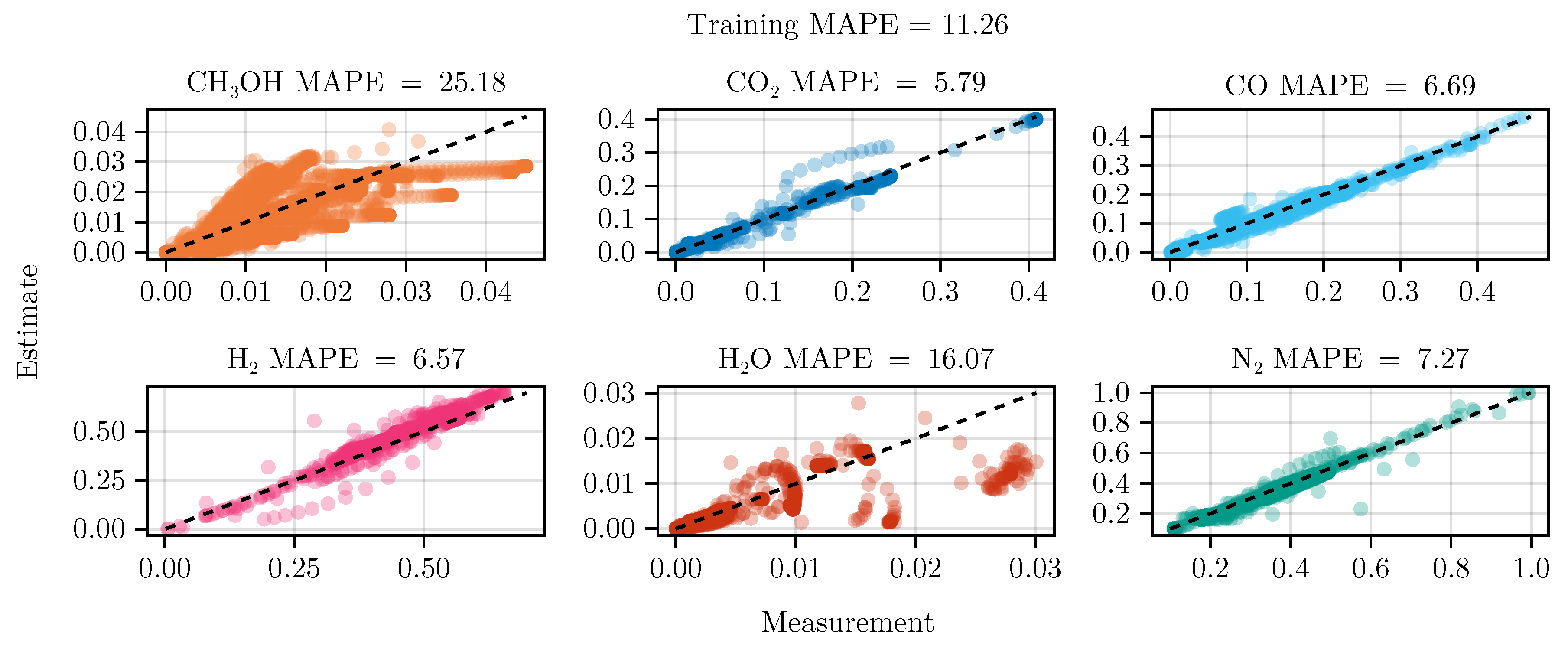
Figure A3.
Parity plot of the fitted mechanistic baseline model over the test data set excluding optimal experimental designs. The color of each species matches the trajectory plots.
Figure A3.
Parity plot of the fitted mechanistic baseline model over the test data set excluding optimal experimental designs. The color of each species matches the trajectory plots.
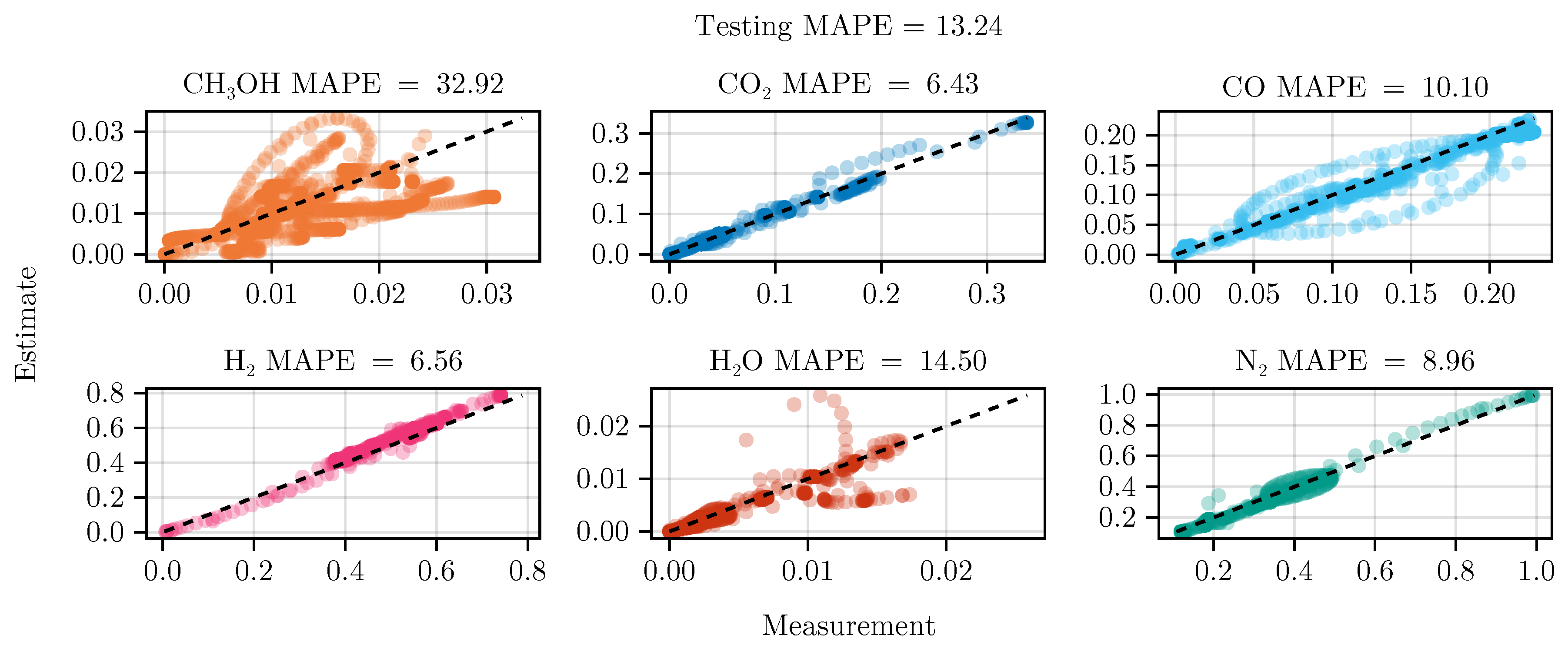
Figure A4.
Parity plot of the fitted mechanistic baseline model over the training data set using optimal experimental designs. The color of each species matches the trajectory plots.
Figure A4.
Parity plot of the fitted mechanistic baseline model over the training data set using optimal experimental designs. The color of each species matches the trajectory plots.
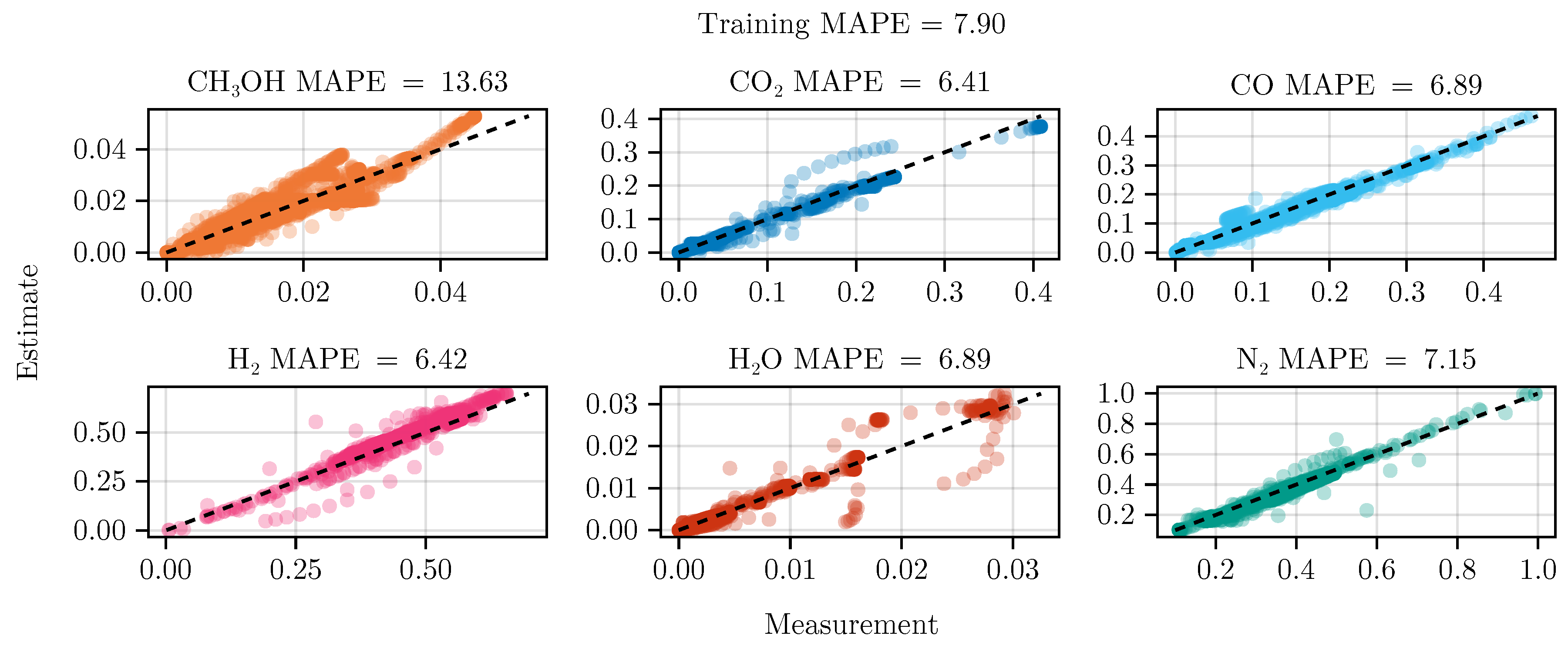
Figure A5.
Parity plot of the fitted mechanistic baseline model over the test data set using optimal experimental designs. The color of each species matches the trajectory plots.
Figure A5.
Parity plot of the fitted mechanistic baseline model over the test data set using optimal experimental designs. The color of each species matches the trajectory plots.

Appendix C.2. Initial Fit
Given that we fitting the model while additional experiments where still conducted, we started with a set of 37 dynamic experiments (MeOH_018 - MeOH_054).
Instead of Equation 12, we initially considered the following optimization problem
with
However, we found that including the species improved the models performance. Prior to the parameter transformation, the positivity of a subset of the parameters was enforced via a penalty approach.
In addition, we used a sequential optimization procedure starting with 1000 iterations Nelder-Mead, to find a better starting position followed with a mesh adaptive direct search via NOMAD to find a set of parameters. Choosing these (gradient-free) optimization algorithms was mainly due to an earlier implementation of the model and objective, which did not allow numerical differentiation. The final version of the model allowed the use of numerical differentiation, hence a more sophisticated method was selected.
Note that we are not particularly interested in an exact estimate at this early stage. The initial estimation is only about finding a sufficient starting point for the optimal experimental design.
Appendix C.3. Data Preparation
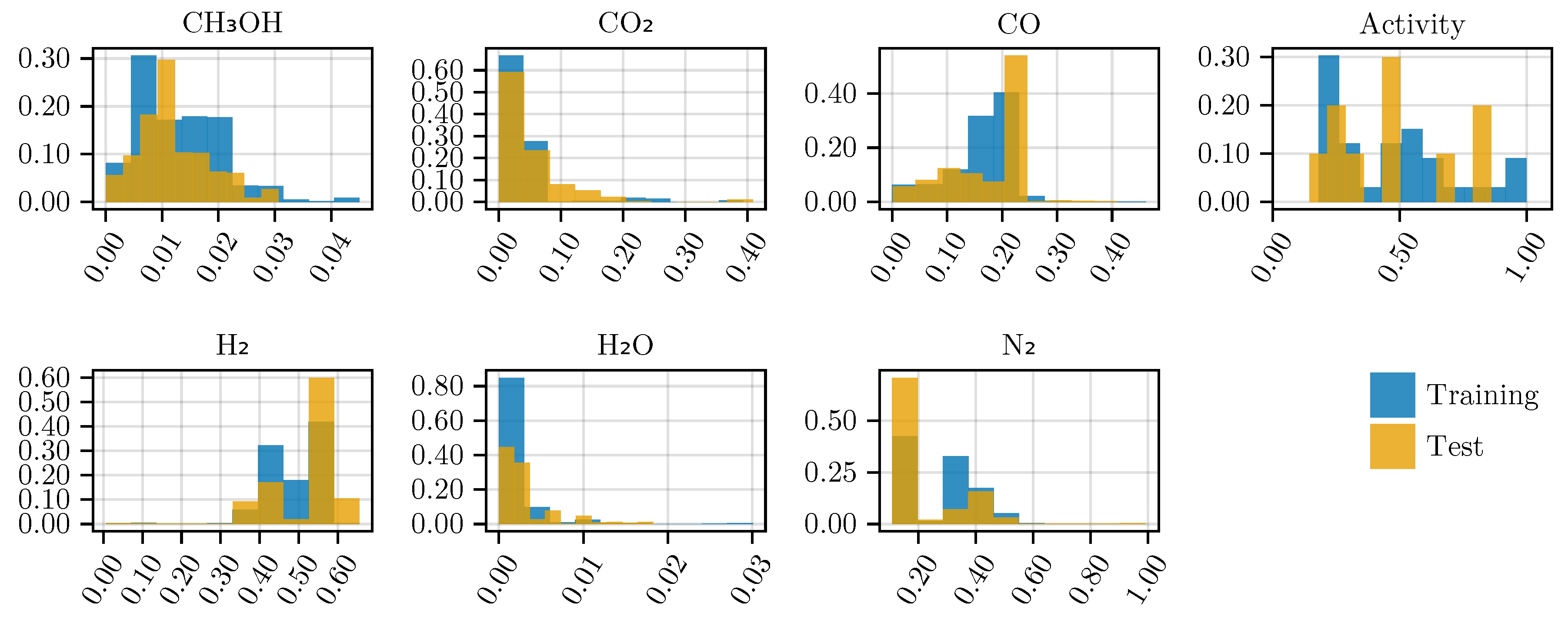
For each experiment, the mean value of observed mole fractions, the measured catalyst activity, the mole fraction of the feed, the nominal volumetric flow rate at the inlet, temperature and pressure were used to stratify the data accordingly. A more detailed assignment of each experiment can be seen in the detailed result tables of Section Appendix C.4.
Figure A6 shows the histogram of the observed mole fractions at the reactor outlet and the catalyst’s activity level.
Figure A6.
Histogram of the mole fractions of the output species and the estimated activity levels for the training and testing data sets. The occurrence is normalized by the probability weight of each bin.
Figure A6.
Histogram of the mole fractions of the output species and the estimated activity levels for the training and testing data sets. The occurrence is normalized by the probability weight of each bin.
Appendix C.4. Model Evaluation
Table A4.
Detailed MAPE values of the mechanistic model (OED) corresponding to Table 4.
Table A4.
Detailed MAPE values of the mechanistic model (OED) corresponding to Table 4.
| Dataset | Experiment | Total | ||||||
|---|---|---|---|---|---|---|---|---|
| Testing | MeOH_025 | 8.27 | 6.33 | 3.41 | 5.59 | 11.5 | 8.96 | 7.35 |
| MeOH_027 | 16.4 | 8.34 | 7.07 | 9.22 | 8.42 | 5.99 | 9.24 | |
| MeOH_033 | 12.3 | 6.55 | 4.07 | 5.5 | 21.5 | 9.04 | 9.84 | |
| MeOH_041 | 12.4 | 6.35 | 13.6 | 5.69 | 10.9 | 9.92 | 9.8 | |
| MeOH_044 | 8.6 | 5.39 | 9.4 | 6.93 | 4.71 | 6.2 | 6.87 | |
| MeOH_044 | 41.4 | 157 | 82.8 | 131 | 8.45 | 7.33 | 71.3 | |
| MeOH_053 | 7.46 | 6.85 | 14.2 | 6.85 | 13.8 | 9.31 | 9.75 | |
| MeOH_054 | 14.8 | 8.82 | 6.79 | 5.12 | 7.28 | 11.1 | 9 | |
| MeOH_076 | 22.1 | 14.7 | 4.66 | 7.37 | 8.94 | 9.73 | 11.2 | |
| MeOH_079 | 12.8 | 7.51 | 3.11 | 6.49 | 16.5 | 9.73 | 9.34 | |
| Training | MeOH_019 | 18.1 | 7.45 | 23.9 | 5.52 | 13.8 | 8.76 | 12.9 |
| MeOH_020 | 15.6 | 6.78 | 10.9 | 4.55 | 4.54 | 7.88 | 8.37 | |
| MeOH_021 | 17.7 | 5.9 | 3.32 | 5.52 | 9.81 | 8.09 | 8.39 | |
| MeOH_022 | 30.6 | 8.07 | 1.16 | 4.04 | 8.76 | 3.24 | 9.32 | |
| MeOH_023 | 5.1 | 6.09 | 1.42 | 5.23 | 2.34 | 8.76 | 4.82 | |
| MeOH_024 | 16.4 | 5.92 | 4.79 | 5.35 | 2.78 | 8.56 | 7.31 | |
| MeOH_026 | 10.8 | 2.84 | 1.47 | 5.66 | 2.97 | 6.1 | 4.97 | |
| MeOH_028 | 23.7 | 6.66 | 5.26 | 6.84 | 12.2 | 4.38 | 9.84 | |
| MeOH_029 | 19.9 | 6.29 | 4.96 | 6.3 | 13.3 | 4.03 | 9.13 | |
| MeOH_030 | 3.59 | 7.08 | 3.43 | 5.89 | 1.79 | 9.12 | 5.15 | |
| MeOH_031 | 2.7 | 6.85 | 2.67 | 5.72 | 0.976 | 9.08 | 4.67 | |
| MeOH_032 | 4.05 | 6.03 | 2.56 | 5.23 | 1.23 | 8.53 | 4.6 | |
| MeOH_034 | 9 | 27.6 | 12.4 | 18.9 | 3.88 | 9.24 | 13.5 | |
| MeOH_035 | 2.55 | 5.71 | 2.2 | 5.16 | 0.947 | 8.98 | 4.26 | |
| MeOH_036 | 12.4 | 11.4 | 4.12 | 5.5 | 1.31 | 8.92 | 7.27 | |
| MeOH_037 | 23.1 | 6.14 | 7.07 | 5.55 | 6.66 | 8.93 | 9.57 | |
| MeOH_038 | 35.9 | 18.5 | 13 | 5.6 | 8.07 | 8.92 | 15 | |
| MeOH_039 | 19.7 | 7.63 | 16 | 8.24 | 9.99 | 10.9 | 12.1 | |
| MeOH_040 | 15.9 | 7.65 | 16.4 | 7.75 | 14.2 | 10.2 | 12 | |
| MeOH_043 | 8.79 | 4.9 | 7.61 | 6.44 | 6.05 | 4.75 | 6.42 | |
| MeOH_045 | 12.7 | 7.49 | 17.1 | 7.69 | 13.4 | 9.88 | 11.4 | |
| MeOH_046 | 9.43 | 6.42 | 10.3 | 7.98 | 5.95 | 6.58 | 7.78 | |
| MeOH_047 | 6.41 | 6.6 | 9.98 | 7.85 | 2.69 | 5.92 | 6.57 | |
| MeOH_048 | 15.8 | 9.66 | 8.74 | 6.96 | 5.31 | 6.13 | 8.77 | |
| MeOH_049 | 8.5 | 6.23 | 8.85 | 7.59 | 4.81 | 5.55 | 6.92 | |
| MeOH_050 | 4.55 | 5.81 | 9.35 | 7.33 | 3.76 | 5.84 | 6.11 | |
| MeOH_051 | 7.86 | 5.24 | 8.32 | 6.45 | 5.95 | 5.83 | 6.61 | |
| MeOH_052 | 8.95 | 5.62 | 8.39 | 6.4 | 4.98 | 5.16 | 6.58 | |
| MeOH_055 | 13.1 | 8.1 | 15.5 | 8.18 | 18.6 | 10.3 | 12.3 | |
| MeOH_073 | 21.6 | 6.81 | 10.7 | 6.97 | 16.4 | 8.93 | 11.9 | |
| MeOH_074 | 8.9 | 16.6 | 4.18 | 7.37 | 10.1 | 9.18 | 9.4 | |
| MeOH_077 | 4.43 | 8.19 | 1.11 | 6.56 | 12.4 | 10.1 | 7.13 | |
| MeOH_081 | 16.8 | 17.6 | 6.65 | 9.51 | 18.7 | 11.3 | 13.4 | |
| MeOH_083 | 16.5 | 14.8 | 3.54 | 7.14 | 19.8 | 9.21 | 11.8 |
Table A5.
Detailed MAPE values of the mechanistic model (NOED) corresponding to Table 4.
Table A5.
Detailed MAPE values of the mechanistic model (NOED) corresponding to Table 4.
| Dataset | Experiment | Total | ||||||
|---|---|---|---|---|---|---|---|---|
| Testing | MeOH_025 | 27.8 | 4.97 | 3.63 | 6.37 | 13.6 | 9.87 | 11 |
| MeOH_027 | 9.84 | 6.54 | 7.91 | 9.5 | 8.55 | 6.44 | 8.13 | |
| MeOH_033 | 89.8 | 7.23 | 1.32 | 5.42 | 15.7 | 8.78 | 21.4 | |
| MeOH_041 | 16.7 | 7.95 | 13.6 | 5.4 | 18.6 | 9.53 | 11.9 | |
| MeOH_042 | 42.8 | 17.8 | 6.17 | 5.3 | 16.3 | 6.17 | 15.8 | |
| MeOH_044 | 34.2 | 8.01 | 7.21 | 5.94 | 15.4 | 5.39 | 12.7 | |
| MeOH_053 | 25.2 | 5.39 | 14.3 | 7.68 | 21.1 | 10.3 | 14 | |
| MeOH_054 | 16 | 8.37 | 6.21 | 4.93 | 9.2 | 11 | 9.27 | |
| MeOH_076 | 37.2 | 33.4 | 5.87 | 7.35 | 17.5 | 9.79 | 18.5 | |
| MeOH_079 | 43.2 | 7.31 | 3.6 | 7.58 | 15 | 10.7 | 14.6 | |
| Training | MeOH_019 | 35.7 | 9.77 | 24.8 | 5.18 | 12.4 | 8.42 | 16.1 |
| MeOH_020 | 16.7 | 6.15 | 10.4 | 5.25 | 7.65 | 8.68 | 9.13 | |
| MeOH_021 | 23.9 | 6.42 | 1.26 | 5.59 | 20.7 | 7.93 | 11 | |
| MeOH_022 | 4.58 | 3.81 | 1.6 | 5.72 | 3.69 | 4.45 | 3.97 | |
| MeOH_023 | 6.2 | 6.33 | 2.37 | 5.32 | 20.1 | 8.76 | 8.18 | |
| MeOH_024 | 27.6 | 6.73 | 4.33 | 5.41 | 16.6 | 8.74 | 11.6 | |
| MeOH_026 | 17 | 2.56 | 0.581 | 5.97 | 16.8 | 6.31 | 8.21 | |
| MeOH_028 | 8.56 | 4.88 | 6.72 | 7.75 | 3.46 | 5.02 | 6.06 | |
| MeOH_029 | 11.1 | 4.68 | 6.4 | 7.17 | 3.23 | 4.67 | 6.21 | |
| MeOH_030 | 7.24 | 7.2 | 1.85 | 6.01 | 20.5 | 9.17 | 8.67 | |
| MeOH_031 | 6.36 | 6.97 | 1.08 | 5.84 | 18.4 | 9.13 | 7.96 | |
| MeOH_032 | 8.43 | 6.12 | 1.1 | 5.35 | 19 | 8.59 | 8.1 | |
| MeOH_034 | 9.78 | 21.7 | 14.9 | 15.1 | 13.1 | 9.44 | 14 | |
| MeOH_035 | 5.86 | 5.76 | 1.01 | 5.28 | 17.2 | 9.06 | 7.35 | |
| MeOH_036 | 18.7 | 8.74 | 2.9 | 5.8 | 23.1 | 9.04 | 11.4 | |
| MeOH_037 | 28.5 | 6.19 | 6.12 | 5.65 | 19.3 | 8.98 | 12.5 | |
| MeOH_038 | 51.5 | 9.55 | 12.6 | 5.97 | 23.7 | 9.08 | 18.7 | |
| MeOH_039 | 14.1 | 7.1 | 14.8 | 8.71 | 23.1 | 11.2 | 13.2 | |
| MeOH_040 | 18.8 | 6.21 | 16.4 | 8.65 | 22.5 | 11.1 | 13.9 | |
| MeOH_043 | 45.5 | 8.33 | 5.7 | 5.13 | 12.7 | 3.79 | 13.5 | |
| MeOH_045 | 21.3 | 6.63 | 16.7 | 8.29 | 23.3 | 10.5 | 14.4 | |
| MeOH_046 | 30 | 8.88 | 8.4 | 7.16 | 15.6 | 5.91 | 12.7 | |
| MeOH_047 | 35.2 | 9.31 | 8.17 | 7.09 | 14.3 | 5.29 | 13.2 | |
| MeOH_048 | 43.4 | 10.6 | 6.97 | 6.04 | 14.4 | 5.65 | 14.5 | |
| MeOH_049 | 39.5 | 8.38 | 7.18 | 6.83 | 12.3 | 4.93 | 13.2 | |
| MeOH_050 | 31.6 | 7.95 | 7.61 | 6.64 | 14.5 | 5.26 | 12.3 | |
| MeOH_051 | 23.4 | 6.83 | 6.77 | 5.93 | 14.4 | 5.37 | 10.5 | |
| MeOH_052 | 36 | 7.47 | 6.87 | 5.68 | 12.4 | 4.6 | 12.2 | |
| MeOH_055 | 33.6 | 6.65 | 16.1 | 9.01 | 22.4 | 11.3 | 16.5 | |
| MeOH_073 | 47.3 | 5.64 | 10.6 | 7.66 | 12.8 | 9.75 | 15.6 | |
| MeOH_074 | 8.15 | 16.9 | 5.53 | 7.34 | 26.2 | 9.11 | 12.2 | |
| MeOH_077 | 8.5 | 8.49 | 1.14 | 6.63 | 11 | 10 | 7.64 | |
| MeOH_081 | 47.3 | 16 | 7.9 | 10.6 | 20.8 | 12.2 | 19.1 | |
| MeOH_083 | 46.6 | 13.9 | 4.47 | 8.8 | 16.6 | 10 | 16.7 |
Appendix D. Hybrid Model Results
Appendix D.1. Hyperparameter Selection
As noted in Table 5, we initially selected the hybrid model based on the coefficient of determination . Later on, we found that this measure was not suitable to clearly capture differences in performance (as now visible in Table 4) or even misleading ( e.g. in the case of the model discrepancy as seen in Figure 9 ). Hence, we switched to a more direct and relatable measure, the mean absolute percentage error (MAPE). Reevaluating the results of the hyperparameter search lead to a slightly different picture, which still included our choosen models in the top ten candidates, but ranked them differently.
Appendix D.2. Detailed Fitting Results
Figure A7.
Trajecotry of MeOH_079 using hybrid model after hyperparameter search and first L-BFGS optimization over the training data set. (INIT)
Figure A7.
Trajecotry of MeOH_079 using hybrid model after hyperparameter search and first L-BFGS optimization over the training data set. (INIT)
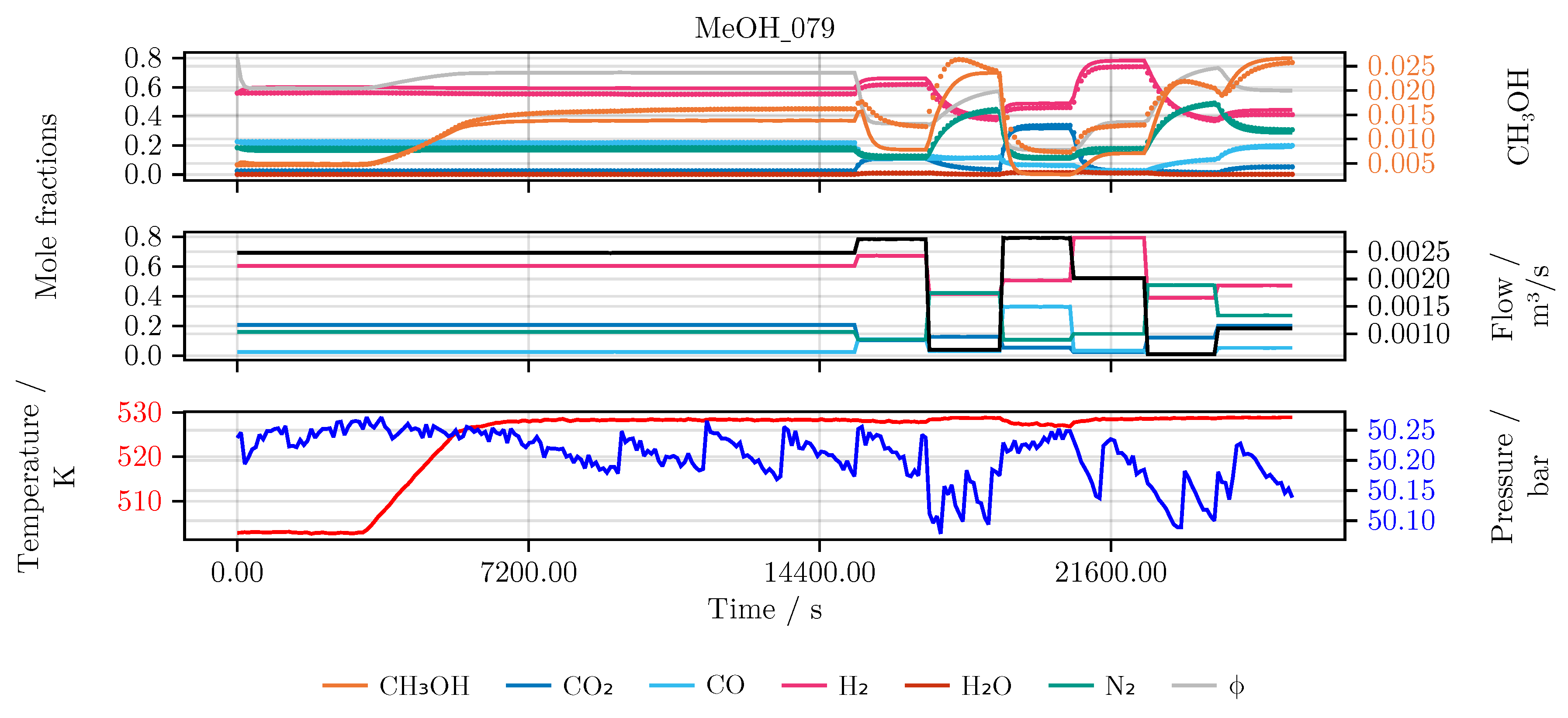
Figure A8.
Parity plot of the hybrid model after hyperparameter search and first L-BFGS optimization over the training data set. (INIT) The color of each species matches the trajectory plots.
Figure A8.
Parity plot of the hybrid model after hyperparameter search and first L-BFGS optimization over the training data set. (INIT) The color of each species matches the trajectory plots.
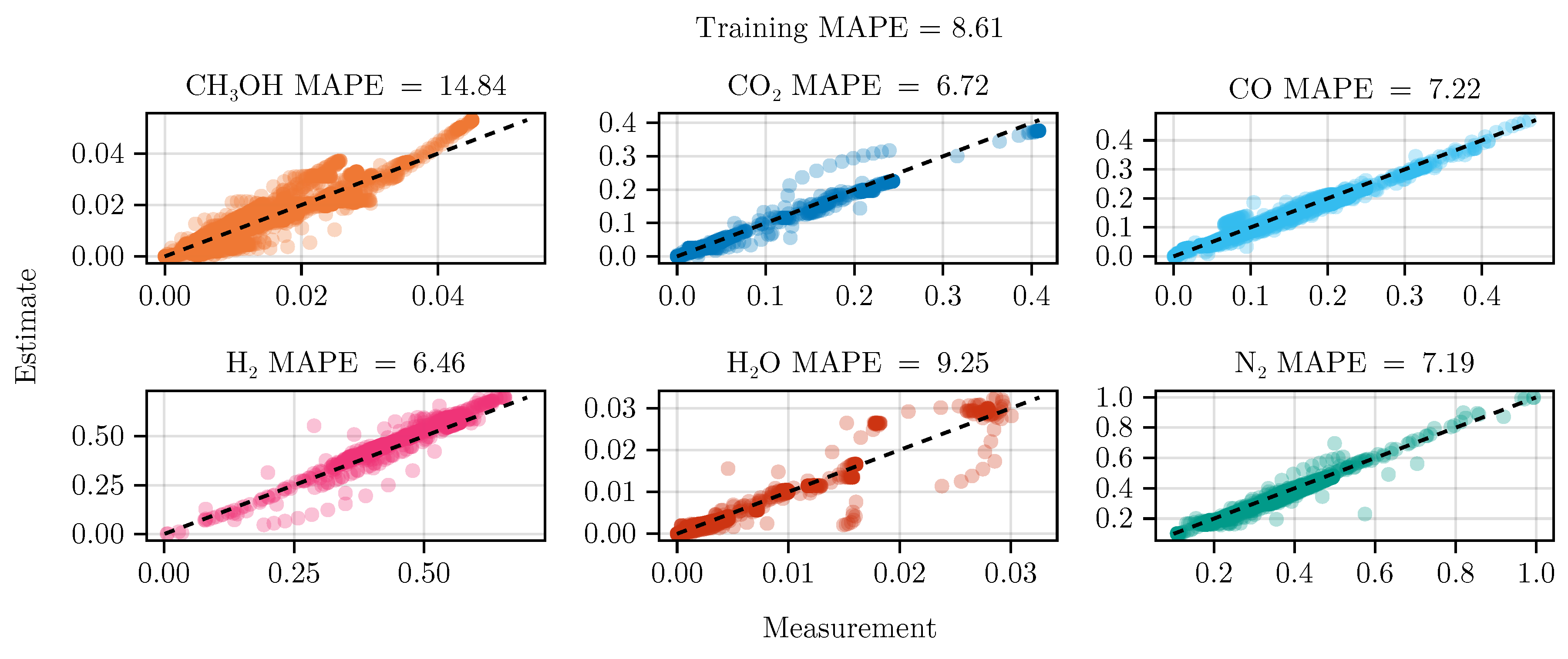
Figure A9.
Parity plot of the hybrid model after hyperparameter search and first L-BFGS optimization over the test data. (INIT) The color of each species matches the trajectory plots.
Figure A9.
Parity plot of the hybrid model after hyperparameter search and first L-BFGS optimization over the test data. (INIT) The color of each species matches the trajectory plots.

Figure A10.
Trajecotry of MeOH_079 using hybrid model after adding experiment MeOH_083 and second L-BFGS optimization over the training data set. (OED)
Figure A10.
Trajecotry of MeOH_079 using hybrid model after adding experiment MeOH_083 and second L-BFGS optimization over the training data set. (OED)
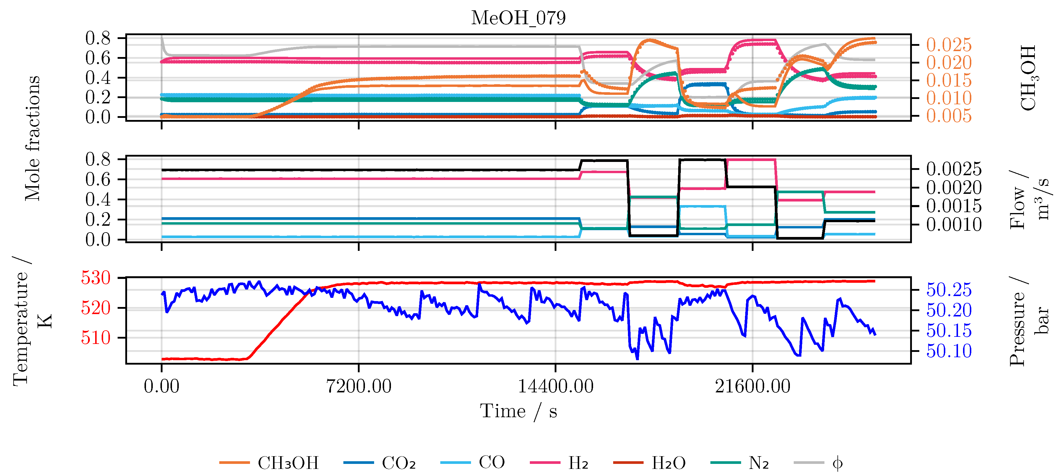
Figure A11.
Parity plot of the hybrid model after adding experiment MeOH_083 and second L-BFGS optimization over the training data set. (OED) The color of each species matches the trajectory plots.
Figure A11.
Parity plot of the hybrid model after adding experiment MeOH_083 and second L-BFGS optimization over the training data set. (OED) The color of each species matches the trajectory plots.

Figure A12.
Parity plot of the fitted hybrid model after adding experiment MeOH_083 and second L-BFGS optimization over the test data set. (OED) The color of each species matches the trajectory plots.
Figure A12.
Parity plot of the fitted hybrid model after adding experiment MeOH_083 and second L-BFGS optimization over the test data set. (OED) The color of each species matches the trajectory plots.
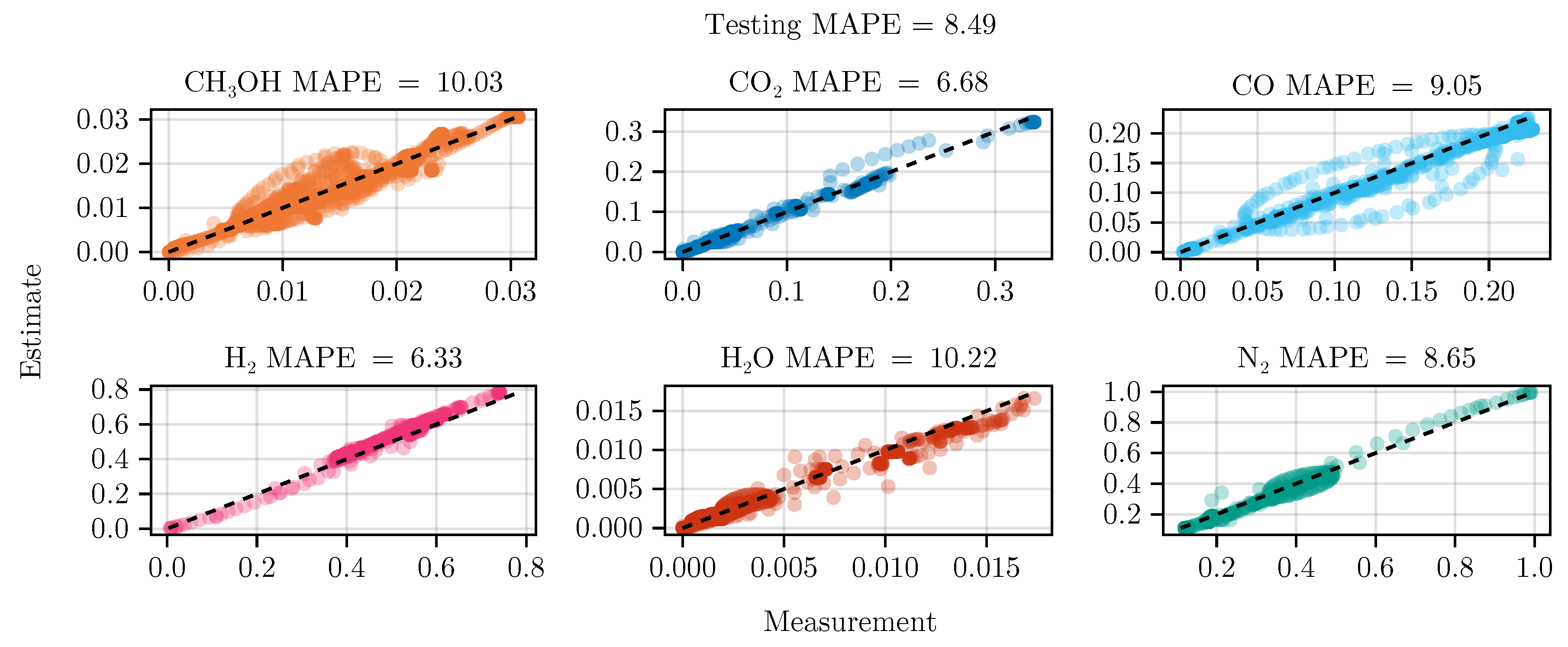
Figure A13.
Trajecotry of MeOH_079 using hybrid model after second L-BFGS optimization over the training data set excluding optimal experimental designs. (NOED)
Figure A13.
Trajecotry of MeOH_079 using hybrid model after second L-BFGS optimization over the training data set excluding optimal experimental designs. (NOED)
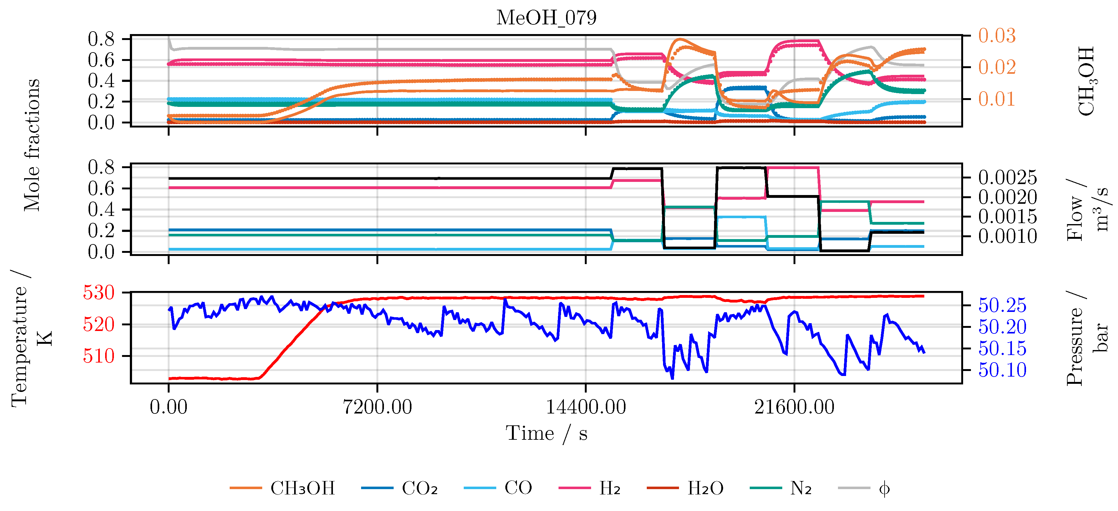
Figure A14.
Parity plot of the hybrid model after second L-BFGS optimization over the training data set excluding optimal experimental designs. (NOED) The color of each species matches the trajectory plots.
Figure A14.
Parity plot of the hybrid model after second L-BFGS optimization over the training data set excluding optimal experimental designs. (NOED) The color of each species matches the trajectory plots.
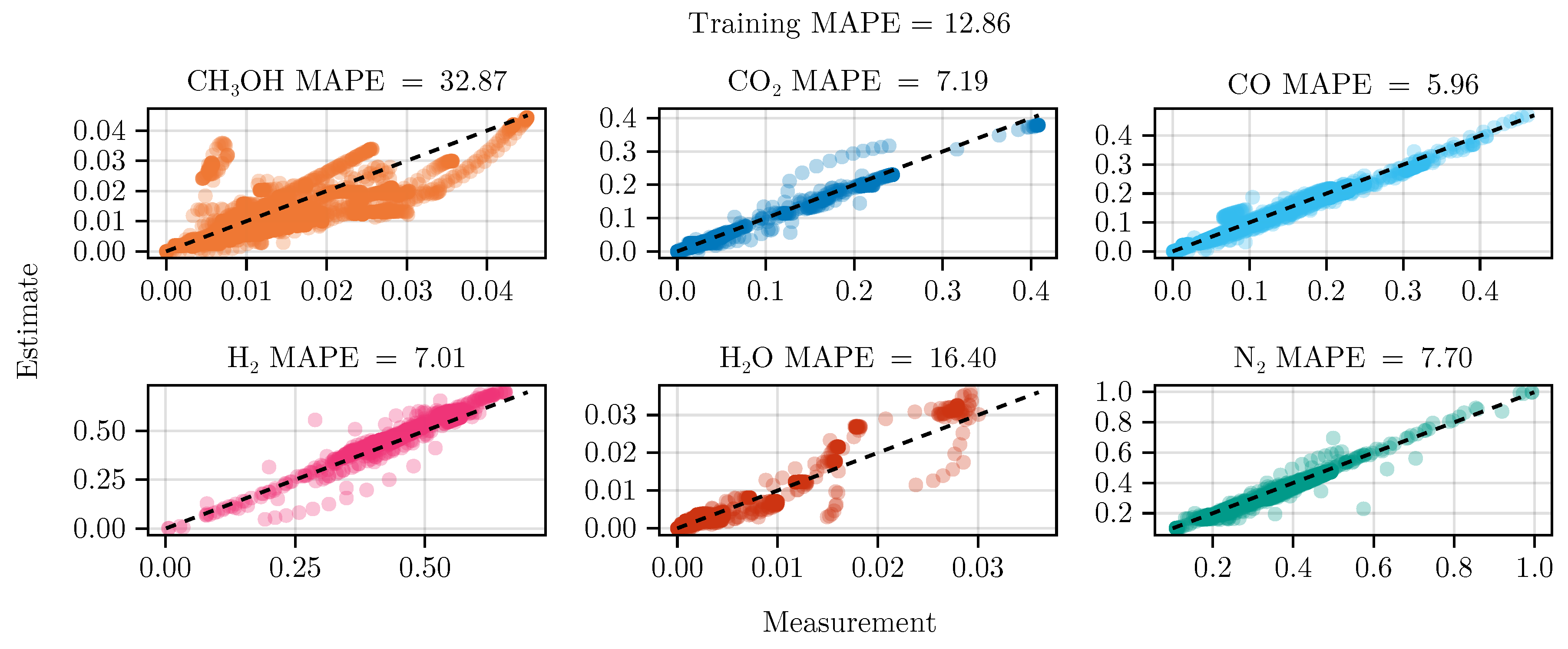
Figure A15.
Parity plot of the hybrid model after second L-BFGS optimization over the test data set excluding optimal experimental designs. (NOED) The color of each species matches the trajectory plots.
Figure A15.
Parity plot of the hybrid model after second L-BFGS optimization over the test data set excluding optimal experimental designs. (NOED) The color of each species matches the trajectory plots.
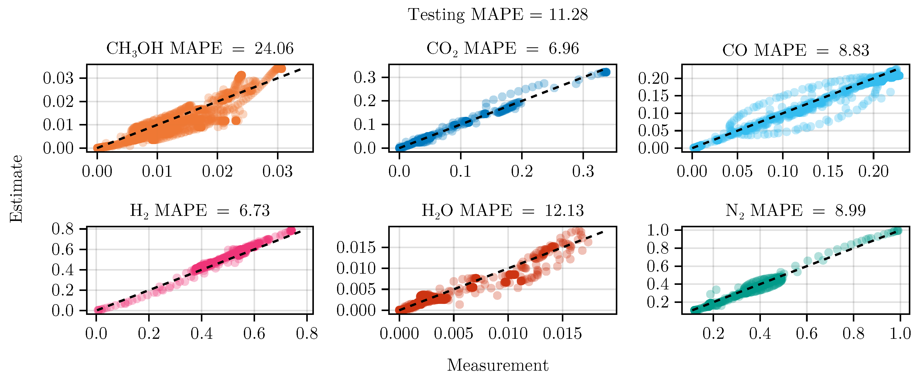
Table A6.
Detailed MAPE values of the hybrid model after hyperparameter search.
| Dataset | Experiment | Total | ||||||
|---|---|---|---|---|---|---|---|---|
| Testing | MeOH_025 | 17.9 | 5.38 | 5.61 | 5.89 | 19.2 | 9.43 | 10.6 |
| MeOH_027 | 32.2 | 8.82 | 7.79 | 8.67 | 9.57 | 5.74 | 12.1 | |
| MeOH_033 | 19.6 | 6.38 | 5.3 | 5.46 | 36.5 | 9.06 | 13.7 | |
| MeOH_041 | 53.8 | 10.1 | 15.4 | 4.33 | 20 | 8.63 | 18.7 | |
| MeOH_042 | 53.1 | 17 | 9.67 | 4.68 | 34.3 | 5.97 | 20.8 | |
| MeOH_044 | 45.5 | 7.17 | 11.7 | 5.43 | 38.7 | 5.35 | 19 | |
| MeOH_053 | 13.1 | 6 | 16.7 | 7.02 | 25.6 | 9.65 | 13 | |
| MeOH_054 | 84.6 | 14.6 | 6.05 | 3.13 | 43.6 | 9.32 | 26.9 | |
| MeOH_076 | 74 | 28.7 | 8.79 | 5.66 | 78.9 | 8.57 | 34.1 | |
| MeOH_079 | 25.5 | 8.06 | 3.84 | 6.11 | 17.7 | 9.58 | 11.8 | |
| Training | MeOH_019 | 77.2 | 11.8 | 22.9 | 3.73 | 48.7 | 7.36 | 28.6 |
| MeOH_020 | 41.6 | 9.75 | 8.07 | 4.08 | 45.4 | 7.25 | 19.4 | |
| MeOH_021 | 12.3 | 5.52 | 5.78 | 5.36 | 39.6 | 8.16 | 12.8 | |
| MeOH_022 | 52.4 | 10.6 | 1.19 | 2.99 | 2.1 | 2.56 | 12 | |
| MeOH_023 | 13.2 | 5.55 | 2.96 | 5.25 | 30 | 8.92 | 11 | |
| MeOH_024 | 79.6 | 8.23 | 7.61 | 3.46 | 61.1 | 7.47 | 27.9 | |
| MeOH_026 | 25.9 | 1.52 | 4.14 | 6.16 | 20.5 | 6.61 | 10.8 | |
| MeOH_028 | 48 | 7.9 | 5.53 | 6.03 | 3.39 | 3.91 | 12.5 | |
| MeOH_029 | 44.5 | 7.51 | 5.29 | 5.49 | 3.56 | 3.55 | 11.6 | |
| MeOH_030 | 12.5 | 6.67 | 5.55 | 5.89 | 20.9 | 9.23 | 10.1 | |
| MeOH_031 | 11.6 | 6.44 | 4.86 | 5.72 | 24.6 | 9.2 | 10.4 | |
| MeOH_032 | 12.9 | 5.62 | 4.62 | 5.23 | 20.9 | 8.65 | 9.65 | |
| MeOH_034 | 11.8 | 27.4 | 13.3 | 19 | 13.5 | 9.3 | 15.7 | |
| MeOH_035 | 8.73 | 5.36 | 3.98 | 5.17 | 18.1 | 9.09 | 8.41 | |
| MeOH_036 | 30.9 | 25.2 | 6.25 | 4.68 | 43.3 | 8.61 | 19.8 | |
| MeOH_037 | 28 | 5.87 | 8.46 | 5.54 | 14.8 | 9 | 11.9 | |
| MeOH_038 | 75.1 | 45.9 | 15.1 | 3.88 | 72 | 8.14 | 36.7 | |
| MeOH_039 | 15.4 | 6.72 | 18.8 | 8.32 | 30.5 | 11.1 | 15.1 | |
| MeOH_040 | 15.7 | 6.41 | 19.1 | 8.08 | 21.3 | 10.7 | 13.6 | |
| MeOH_043 | 60.6 | 7.88 | 9.56 | 4.45 | 37.2 | 3.59 | 20.5 | |
| MeOH_045 | 18.4 | 6.56 | 19.7 | 7.87 | 20.1 | 10.2 | 13.8 | |
| MeOH_046 | 47.3 | 8.51 | 12.8 | 6.52 | 35.3 | 5.74 | 19.4 | |
| MeOH_047 | 53.1 | 8.78 | 12.3 | 6.3 | 37 | 5.06 | 20.4 | |
| MeOH_048 | 55.3 | 10.4 | 11 | 5.47 | 39.3 | 5.53 | 21.2 | |
| MeOH_049 | 53.2 | 7.75 | 11 | 6.25 | 38.7 | 4.8 | 20.3 | |
| MeOH_050 | 47.3 | 7.36 | 11.7 | 5.97 | 36.5 | 5.08 | 19 | |
| MeOH_051 | 43.1 | 6.71 | 11 | 5.24 | 34.6 | 5.13 | 17.6 | |
| MeOH_052 | 51.4 | 6.91 | 10.7 | 5.09 | 38.4 | 4.45 | 19.5 | |
| MeOH_055 | 22.8 | 7.16 | 17.8 | 8.43 | 16.7 | 10.7 | 14 | |
| MeOH_073 | 12.8 | 6.44 | 10.9 | 6.85 | 19.5 | 8.97 | 10.9 | |
| MeOH_074 | 5.59 | 16.1 | 7.06 | 7.23 | 24.7 | 9.1 | 11.6 | |
| MeOH_077 | 4.54 | 7.9 | 3.83 | 6.44 | 41.2 | 10.1 | 12.3 | |
| MeOH_081 | 33.1 | 17 | 7.7 | 9.19 | 22.9 | 11.3 | 16.9 | |
| MeOH_083 | 26.8 | 22.2 | 4.67 | 6.96 | 27.2 | 9.3 | 16.2 |
Table A7.
Detailed MAPE values of the hybrid model (INIT) corresponding to Table 4.
Table A7.
Detailed MAPE values of the hybrid model (INIT) corresponding to Table 4.
| Dataset | Experiment | Total | ||||||
|---|---|---|---|---|---|---|---|---|
| Testing | MeOH_025 | 8.13 | 6.29 | 3.93 | 5.55 | 11 | 8.95 | 7.32 |
| MeOH_027 | 14.8 | 8.02 | 7.24 | 9.27 | 10.6 | 6.07 | 9.35 | |
| MeOH_033 | 15 | 6.51 | 4.57 | 5.46 | 27.8 | 9.03 | 11.4 | |
| MeOH_041 | 20.3 | 5.75 | 14 | 5.94 | 11.9 | 10.2 | 11.3 | |
| MeOH_042 | 14.2 | 16 | 7.58 | 6.63 | 10.1 | 6.76 | 10.2 | |
| MeOH_044 | 9.29 | 5.33 | 9.07 | 7.04 | 7.55 | 6.23 | 7.42 | |
| MeOH_053 | 5.48 | 6.93 | 14.6 | 6.76 | 13 | 9.22 | 9.34 | |
| MeOH_054 | 28.4 | 7.36 | 6.84 | 5.33 | 11.7 | 11.4 | 11.8 | |
| MeOH_076 | 31.1 | 23.9 | 5.03 | 7.46 | 13.9 | 9.87 | 15.2 | |
| MeOH_079 | 15.8 | 7.39 | 3.21 | 6.54 | 15 | 9.78 | 9.62 | |
| Training | MeOH_019 | 25.4 | 7.36 | 23.6 | 5.82 | 21.8 | 9.05 | 15.5 |
| MeOH_020 | 22.7 | 7.81 | 10.4 | 4.54 | 8.11 | 7.89 | 10.2 | |
| MeOH_021 | 15.8 | 5.88 | 3.92 | 5.38 | 17.6 | 8.07 | 9.44 | |
| MeOH_022 | 26.2 | 7.12 | 1.15 | 4.38 | 10.3 | 3.47 | 8.78 | |
| MeOH_023 | 4.01 | 6.02 | 1.3 | 5.18 | 11.1 | 8.74 | 6.06 | |
| MeOH_024 | 32 | 4.72 | 5.38 | 5.55 | 9.04 | 8.78 | 10.9 | |
| MeOH_026 | 12.3 | 2.63 | 2.29 | 5.68 | 5.45 | 6.15 | 5.75 | |
| MeOH_028 | 20.7 | 6.21 | 5.33 | 7.09 | 13.3 | 4.52 | 9.51 | |
| MeOH_029 | 18.6 | 5.89 | 5 | 6.5 | 14.3 | 4.16 | 9.08 | |
| MeOH_030 | 2.8 | 7 | 4.16 | 5.85 | 7 | 9.11 | 5.99 | |
| MeOH_031 | 1.92 | 6.77 | 3.45 | 5.68 | 9.97 | 9.07 | 6.14 | |
| MeOH_032 | 3.29 | 5.94 | 3.32 | 5.19 | 7.59 | 8.53 | 5.64 | |
| MeOH_034 | 8.59 | 21.1 | 15.4 | 15.3 | 7.97 | 9.49 | 13 | |
| MeOH_035 | 2.44 | 5.62 | 2.97 | 5.12 | 7.69 | 8.98 | 5.47 | |
| MeOH_036 | 19.5 | 15.3 | 4.66 | 5.51 | 6.72 | 8.97 | 10.1 | |
| MeOH_037 | 20 | 6.09 | 7.74 | 5.51 | 6.58 | 8.91 | 9.13 | |
| MeOH_038 | 43.5 | 26.5 | 13.3 | 5.69 | 9.09 | 9.02 | 17.9 | |
| MeOH_039 | 16.8 | 7.8 | 16.1 | 8.09 | 10 | 10.7 | 11.6 | |
| MeOH_040 | 14.4 | 7.7 | 16.8 | 7.66 | 11.6 | 10.1 | 11.4 | |
| MeOH_043 | 11.5 | 4.67 | 7.07 | 6.65 | 8.68 | 4.85 | 7.23 | |
| MeOH_045 | 11.1 | 7.49 | 17.6 | 7.62 | 10 | 9.84 | 10.6 | |
| MeOH_046 | 10.6 | 6.4 | 9.97 | 8.08 | 9.31 | 6.61 | 8.5 | |
| MeOH_047 | 7.77 | 6.51 | 9.58 | 8.01 | 8.44 | 5.97 | 7.71 | |
| MeOH_048 | 17.3 | 9.58 | 8.37 | 7.09 | 7.34 | 6.17 | 9.31 | |
| MeOH_049 | 9.56 | 6.13 | 8.53 | 7.63 | 7.1 | 5.62 | 7.43 | |
| MeOH_050 | 6.17 | 5.8 | 9.01 | 7.43 | 8.68 | 5.88 | 7.16 | |
| MeOH_051 | 9.81 | 5.24 | 8.04 | 6.52 | 9.2 | 5.87 | 7.45 | |
| MeOH_052 | 8.06 | 5.56 | 8.11 | 6.51 | 6.94 | 5.2 | 6.73 | |
| MeOH_055 | 12 | 8.05 | 16.1 | 8.12 | 14.6 | 10.3 | 11.5 | |
| MeOH_073 | 11.5 | 7.07 | 10.7 | 6.49 | 15.9 | 8.57 | 10 | |
| MeOH_074 | 3.76 | 16.4 | 4.34 | 7.32 | 11.5 | 9.08 | 8.73 | |
| MeOH_077 | 8.3 | 8.17 | 1.81 | 6.5 | 20.4 | 10 | 9.2 | |
| MeOH_081 | 20.5 | 20.4 | 6.84 | 9.51 | 17.2 | 11.4 | 14.3 | |
| MeOH_083 | 16.1 | 15.3 | 3.85 | 7.21 | 17.8 | 9.23 | 11.6 |
Table A8.
Detailed MAPE values of the hybrid model (OED) corresponding to Table 4.
Table A8.
Detailed MAPE values of the hybrid model (OED) corresponding to Table 4.
| Dataset | Experiment | Total | ||||||
|---|---|---|---|---|---|---|---|---|
| Testing | MeOH_025 | 27.7 | 5.74 | 4.11 | 5.87 | 4.4 | 9.33 | 9.52 |
| MeOH_027 | 18 | 8.37 | 6.98 | 9.1 | 8.74 | 5.96 | 9.52 | |
| MeOH_033 | 30.6 | 6.53 | 1.58 | 5.82 | 19.7 | 9.28 | 12.3 | |
| MeOH_041 | 24.5 | 5.3 | 14.5 | 5.96 | 7.1 | 10.4 | 11.3 | |
| MeOH_042 | 21.9 | 15.1 | 8.97 | 7.01 | 14.9 | 7 | 12.5 | |
| MeOH_044 | 9.86 | 5.74 | 9.4 | 6.71 | 5.16 | 6.05 | 7.15 | |
| MeOH_053 | 29.7 | 6.47 | 14.6 | 7.06 | 11.7 | 9.57 | 13.2 | |
| MeOH_054 | 17.9 | 10.5 | 7.31 | 5.25 | 12.6 | 11.2 | 10.8 | |
| MeOH_076 | 32.4 | 17.8 | 4.2 | 7.48 | 13.2 | 9.74 | 14.1 | |
| MeOH_079 | 18.8 | 8.15 | 2.43 | 6.53 | 15.9 | 9.74 | 10.3 | |
| Training | MeOH_019 | 34.1 | 8.44 | 23 | 5.56 | 28.7 | 9.1 | 18.2 |
| MeOH_020 | 30.8 | 6.45 | 5.87 | 5.33 | 31.3 | 9.12 | 14.8 | |
| MeOH_021 | 32.4 | 5.3 | 2.81 | 5.73 | 8.39 | 8.63 | 10.6 | |
| MeOH_022 | 24.5 | 7.24 | 1.16 | 4.37 | 3.41 | 3.49 | 7.37 | |
| MeOH_023 | 38.9 | 5.18 | 1.01 | 5.74 | 10.8 | 9.39 | 11.8 | |
| MeOH_024 | 32.1 | 9.86 | 5.35 | 5.44 | 8.12 | 8.7 | 11.6 | |
| MeOH_026 | 40.8 | 1.33 | 4.25 | 6.75 | 16.1 | 7.11 | 12.7 | |
| MeOH_028 | 10.8 | 6.11 | 5.56 | 7.29 | 10.3 | 4.65 | 7.46 | |
| MeOH_029 | 7.61 | 5.89 | 5.14 | 6.73 | 13.1 | 4.29 | 7.12 | |
| MeOH_030 | 37.1 | 6.65 | 2.47 | 6.27 | 17.7 | 9.52 | 13.3 | |
| MeOH_031 | 36.4 | 6.4 | 1.78 | 6.11 | 14.6 | 9.5 | 12.5 | |
| MeOH_032 | 35.1 | 5.6 | 1.74 | 5.6 | 15.3 | 8.92 | 12 | |
| MeOH_034 | 20.5 | 27.5 | 11.8 | 19.1 | 12.2 | 9.42 | 16.7 | |
| MeOH_035 | 31.3 | 5.42 | 0.973 | 5.48 | 20.1 | 9.3 | 12.1 | |
| MeOH_036 | 28.7 | 11.7 | 2.7 | 5.87 | 22.5 | 9.14 | 13.4 | |
| MeOH_037 | 37 | 6 | 6.11 | 5.76 | 21.7 | 9.12 | 14.3 | |
| MeOH_038 | 22.8 | 15.4 | 12.3 | 5.8 | 18.6 | 8.82 | 13.9 | |
| MeOH_039 | 37.5 | 5.13 | 19.1 | 9.29 | 20 | 12.2 | 17.2 | |
| MeOH_040 | 33.1 | 5.31 | 19.3 | 8.74 | 12.8 | 11.4 | 15.1 | |
| MeOH_043 | 18.9 | 3.79 | 8.48 | 7.07 | 22.1 | 5.23 | 10.9 | |
| MeOH_045 | 37.9 | 5.81 | 19 | 8.45 | 6.41 | 10.8 | 14.7 | |
| MeOH_046 | 25.4 | 5.33 | 10.6 | 8.61 | 18.8 | 7.08 | 12.6 | |
| MeOH_047 | 23.4 | 5.5 | 10.2 | 8.4 | 8.09 | 6.33 | 10.3 | |
| MeOH_048 | 22.4 | 9.52 | 8.91 | 7.61 | 17.2 | 6.51 | 12 | |
| MeOH_049 | 22.8 | 5.38 | 8.95 | 8.17 | 16.6 | 5.98 | 11.3 | |
| MeOH_050 | 26 | 4.91 | 9.26 | 7.92 | 14.1 | 6.27 | 11.4 | |
| MeOH_051 | 27.8 | 4.75 | 7.73 | 7.02 | 21 | 6.24 | 12.4 | |
| MeOH_052 | 24.1 | 4.96 | 8.11 | 7.02 | 18.7 | 5.58 | 11.4 | |
| MeOH_055 | 36.6 | 6.92 | 16.6 | 8.75 | 14.1 | 11 | 15.7 | |
| MeOH_073 | 122 | 7.71 | 10.1 | 5.24 | 15.5 | 7.68 | 28.1 | |
| MeOH_074 | 38 | 16.8 | 5.43 | 7.69 | 12.9 | 9.69 | 15.1 | |
| MeOH_077 | 33.1 | 7.95 | 1.16 | 6.99 | 16.2 | 10.4 | 12.6 | |
| MeOH_081 | 22.6 | 14.4 | 6.95 | 9.42 | 19.3 | 11.3 | 14 | |
| MeOH_083 | 18.3 | 13 | 3.63 | 7.32 | 20 | 9.3 | 11.9 |
Table A9.
Detailed MAPE values of the hybrid model (NOED) corresponding to Table 4.
Table A9.
Detailed MAPE values of the hybrid model (NOED) corresponding to Table 4.
| Dataset | Experiment | Total | ||||||
|---|---|---|---|---|---|---|---|---|
| Testing | MeOH_025 | 27.7 | 5.74 | 4.11 | 5.87 | 4.4 | 9.33 | 9.52 |
| MeOH_027 | 18 | 7.59 | 7.38 | 9.64 | 8.87 | 6.32 | 9.63 | |
| MeOH_033 | 30.6 | 6.53 | 1.58 | 5.82 | 19.7 | 9.28 | 12.3 | |
| MeOH_041 | 24.5 | 5.3 | 14.5 | 5.96 | 7.1 | 10.4 | 11.3 | |
| MeOH_042 | 21.9 | 15.1 | 8.97 | 7.01 | 14.9 | 7 | 12.5 | |
| MeOH_044 | 26.3 | 4.23 | 10.3 | 7.59 | 17.1 | 6.76 | 12 | |
| MeOH_053 | 29.7 | 6.47 | 14.6 | 7.06 | 11.7 | 9.57 | 13.2 | |
| MeOH_054 | 17.9 | 10.5 | 7.31 | 5.25 | 12.6 | 11.2 | 10.8 | |
| MeOH_076 | 32.4 | 17.8 | 4.2 | 7.48 | 13.2 | 9.74 | 14.1 | |
| MeOH_079 | 18.8 | 8.15 | 2.43 | 6.53 | 15.9 | 9.74 | 10.3 | |
| Training | MeOH_019 | 34.1 | 8.44 | 23 | 5.56 | 28.7 | 9.1 | 18.2 |
| MeOH_020 | 30.8 | 6.45 | 5.87 | 5.33 | 31.3 | 9.12 | 14.8 | |
| MeOH_021 | 32.4 | 5.3 | 2.81 | 5.73 | 8.39 | 8.63 | 10.6 | |
| MeOH_022 | 24.5 | 7.24 | 1.16 | 4.37 | 3.41 | 3.49 | 7.37 | |
| MeOH_023 | 38.9 | 5.18 | 1.01 | 5.74 | 10.8 | 9.39 | 11.8 | |
| MeOH_024 | 32.1 | 9.86 | 5.35 | 5.44 | 8.12 | 8.7 | 11.6 | |
| MeOH_026 | 40.8 | 1.33 | 4.25 | 6.75 | 16.1 | 7.11 | 12.7 | |
| MeOH_028 | 10.8 | 6.11 | 5.56 | 7.29 | 10.3 | 4.65 | 7.46 | |
| MeOH_029 | 7.61 | 5.89 | 5.14 | 6.73 | 13.1 | 4.29 | 7.12 | |
| MeOH_030 | 37.1 | 6.65 | 2.47 | 6.27 | 17.7 | 9.52 | 13.3 | |
| MeOH_031 | 36.4 | 6.4 | 1.78 | 6.11 | 14.6 | 9.5 | 12.5 | |
| MeOH_032 | 35.1 | 5.6 | 1.74 | 5.6 | 15.3 | 8.92 | 12 | |
| MeOH_034 | 20.5 | 27.5 | 11.8 | 19.1 | 12.2 | 9.42 | 16.7 | |
| MeOH_035 | 31.3 | 5.42 | 0.973 | 5.48 | 20.1 | 9.3 | 12.1 | |
| MeOH_036 | 28.7 | 11.7 | 2.7 | 5.87 | 22.5 | 9.14 | 13.4 | |
| MeOH_037 | 37 | 6 | 6.11 | 5.76 | 21.7 | 9.12 | 14.3 | |
| MeOH_038 | 22.8 | 15.4 | 12.3 | 5.8 | 18.6 | 8.82 | 13.9 | |
| MeOH_039 | 37.5 | 5.13 | 19.1 | 9.29 | 20 | 12.2 | 17.2 | |
| MeOH_040 | 33.1 | 5.31 | 19.3 | 8.74 | 12.8 | 11.4 | 15.1 | |
| MeOH_043 | 18.9 | 3.79 | 8.48 | 7.07 | 22.1 | 5.23 | 10.9 | |
| MeOH_045 | 37.9 | 5.81 | 19 | 8.45 | 6.41 | 10.8 | 14.7 | |
| MeOH_046 | 25.4 | 5.33 | 10.6 | 8.61 | 18.8 | 7.08 | 12.6 | |
| MeOH_047 | 23.4 | 5.5 | 10.2 | 8.4 | 8.09 | 6.33 | 10.3 | |
| MeOH_048 | 22.4 | 9.52 | 8.91 | 7.61 | 17.2 | 6.51 | 12 | |
| MeOH_049 | 22.8 | 5.38 | 8.95 | 8.17 | 16.6 | 5.98 | 11.3 | |
| MeOH_050 | 26 | 4.91 | 9.26 | 7.92 | 14.1 | 6.27 | 11.4 | |
| MeOH_051 | 27.8 | 4.75 | 7.73 | 7.02 | 21 | 6.24 | 12.4 | |
| MeOH_052 | 24.1 | 4.96 | 8.11 | 7.02 | 18.7 | 5.58 | 11.4 | |
| MeOH_055 | 36.6 | 6.92 | 16.6 | 8.75 | 14.1 | 11 | 15.7 | |
| MeOH_073 | 122 | 7.71 | 10.1 | 5.24 | 15.5 | 7.68 | 28.1 | |
| MeOH_074 | 38 | 16.8 | 5.43 | 7.69 | 12.9 | 9.69 | 15.1 | |
| MeOH_077 | 33.1 | 7.95 | 1.16 | 6.99 | 16.2 | 10.4 | 12.6 | |
| MeOH_081 | 22.6 | 14.4 | 6.95 | 9.42 | 19.3 | 11.3 | 14 | |
| MeOH_083 | 18.3 | 13 | 3.63 | 7.32 | 20 | 9.3 | 11.9 |
Appendix E. Optimal Experimental Design
Appendix E.1. Optimal Experimental Design as Optimal Control
As described in [31] we formulate the optimal experimental design problem as the following optimal control problem:
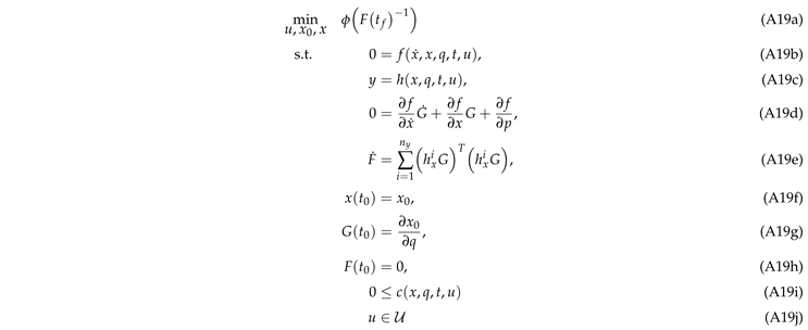
In Equation A19 a suitable criterion based on the variance-covariance matrix of the unknown or uncertain parameters is minimized. To this end, different criteria have been proposed, typically related to the volume of the confidence ellipsoid of the associated parameters p. The most commonly used criteria are the A-Criterion (trace of ), the D-Criterion (determinant of ), and the E-Criterion (maximum eigenvalue of ). The degrees of freedom are controls and potentially also the initial conditions on the differential states. The dynamics of the original DAE system are incorporated in A19b. The dynamics of the Fisher information matrix F is given by the weighted sum of observability Gramians for each observed function in A19e. Here denotes the forward sensitivities of the states x with respect to the parameters q as given in A19d. Also general constraints may be present to model path constraints in A19i.
Given the Equation A19, we need to solve an augmented system of differential equations with states. Using the fact that F is positive semidefinite and symmetric, we only need to add state variables to model its dynamics, which in total leads to states, i.e., the size of the augmented system scales quadratically with the number of parameters .
Appendix E.2. OED for Physical Parameters
After a first re-calibration of the mechanistic model described in Section Appendix C, we computed four optimal experimental designs for different subsets of model parameters in order to collect insightful data to reduce parameter uncertainty. The specific parameters for which we compute experimental designs are the two parameters in the Arrhenius equation of each of the three elementary reactions, i.e., CO and CO2-hydrogenation and RWGS reaction, and the two rate constants in the kinetic equation for the state .
The solutions to the four experimental design problems are illustrated in Figure A16–Figure A19.
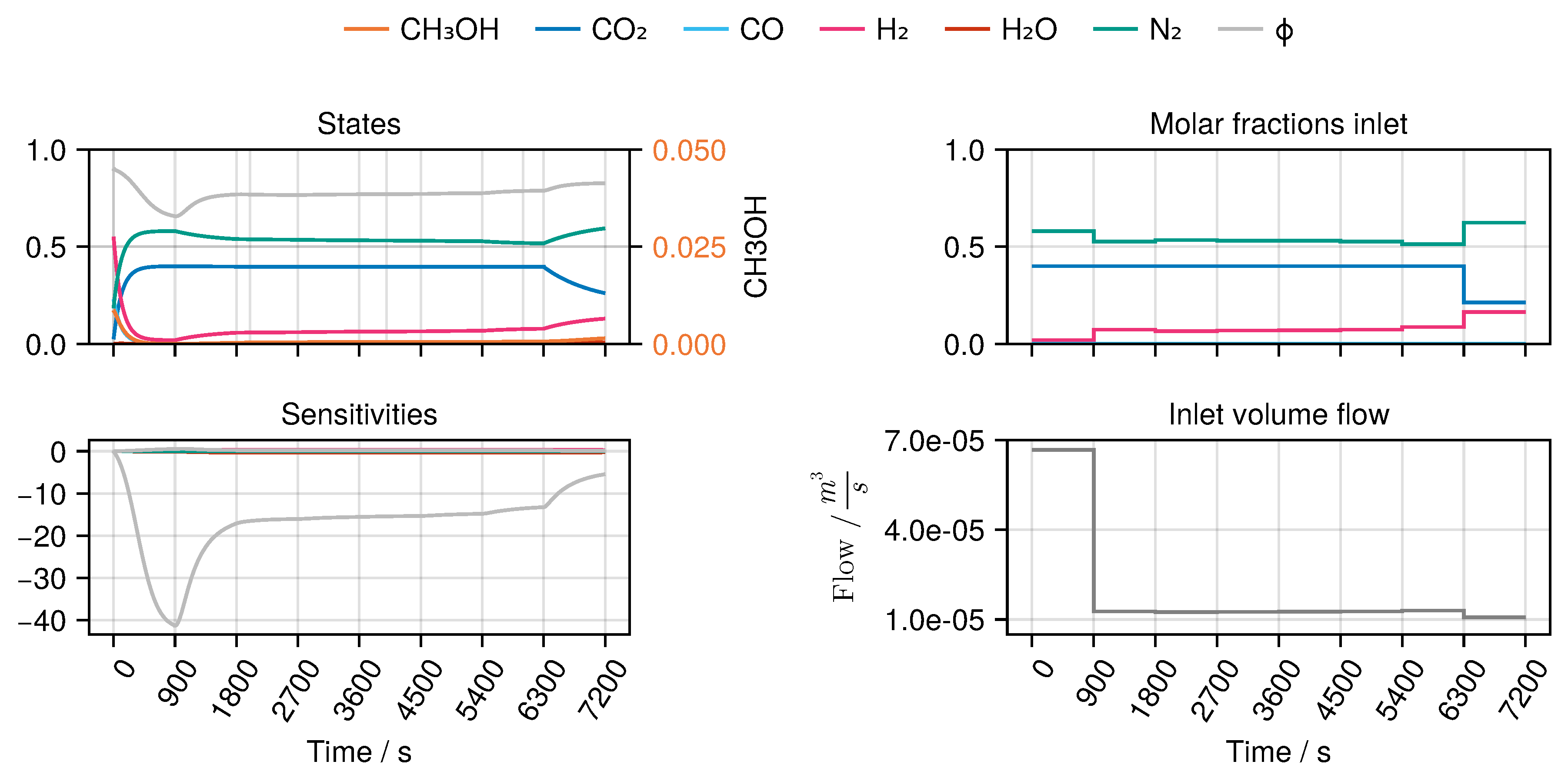
In the optimal design for the CO hydrogenation (Figure A16) no CO2 is present in the feed. Thus, the CO hydrogenation is the only reaction in this experiment yielding specific information for this reaction kinetics. The design for the CO2 hydrogenation (Figure A17) is an interesting result. Switching between one feed containing the reactants CO2 and H2 of the desired reaction and another feed completely without both was suggested. Thus, a broad range of reactant concentrations is included in the experiment. In the RWGS design (Figure A18) no CO is present in the feed, forcing the reverse path of the reaction. Interestingly, in the first time period of the experiment all carbon species are purged out of the reactor with N2 and H2. In the design for the reversible conversion of active catalytic sites (Figure A19) first a low reduction potential via a low hydrogen concentration (and no CO) is applied which is later on increased in the experiment to influence the state . All in all, the optimal experiments are qualitatively meaningful with regard to their design purpose, but nevertheless not trivial in their specific quantitative design.
Figure A16.
Experimental design for estimating parameters in Arrhenius equation of the hydrogenation. The temperature was determined as °C.
Figure A16.
Experimental design for estimating parameters in Arrhenius equation of the hydrogenation. The temperature was determined as °C.
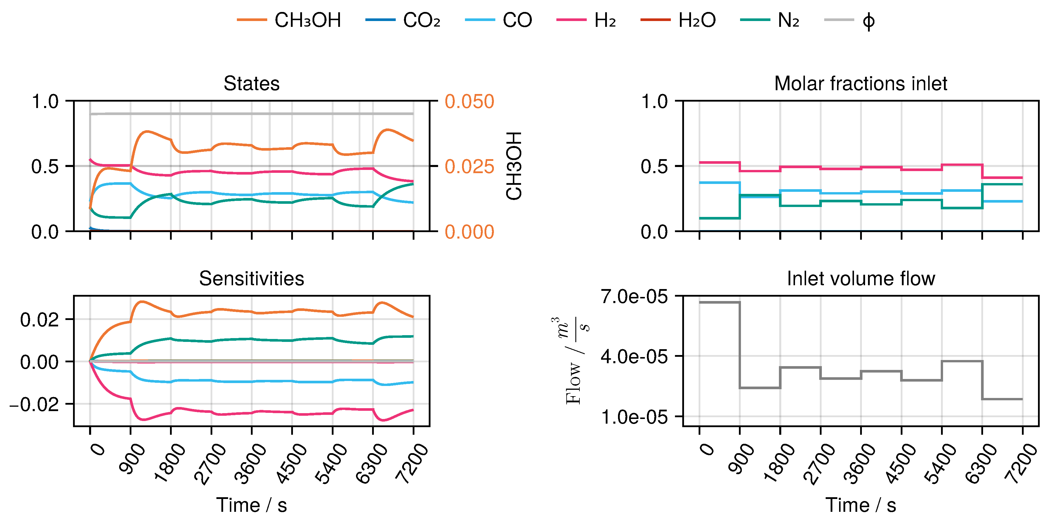
Figure A17.
As in Figure A16, but for the hydrogenation. The temperature was determined as °C.
Figure A17.
As in Figure A16, but for the hydrogenation. The temperature was determined as °C.
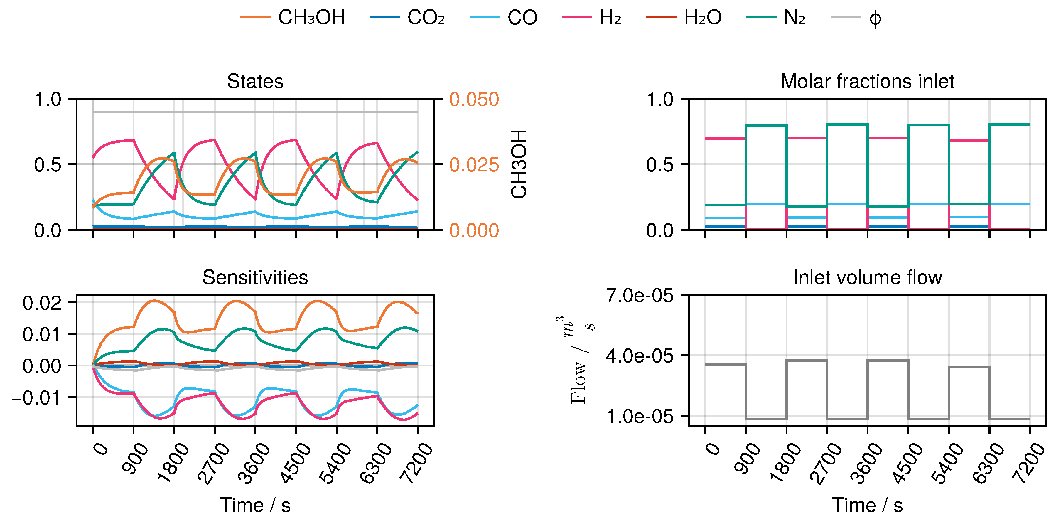
Figure A18.
As in Figure A16, but for the RWGS reaction. The temperature was determined as °C.
Figure A18.
As in Figure A16, but for the RWGS reaction. The temperature was determined as °C.
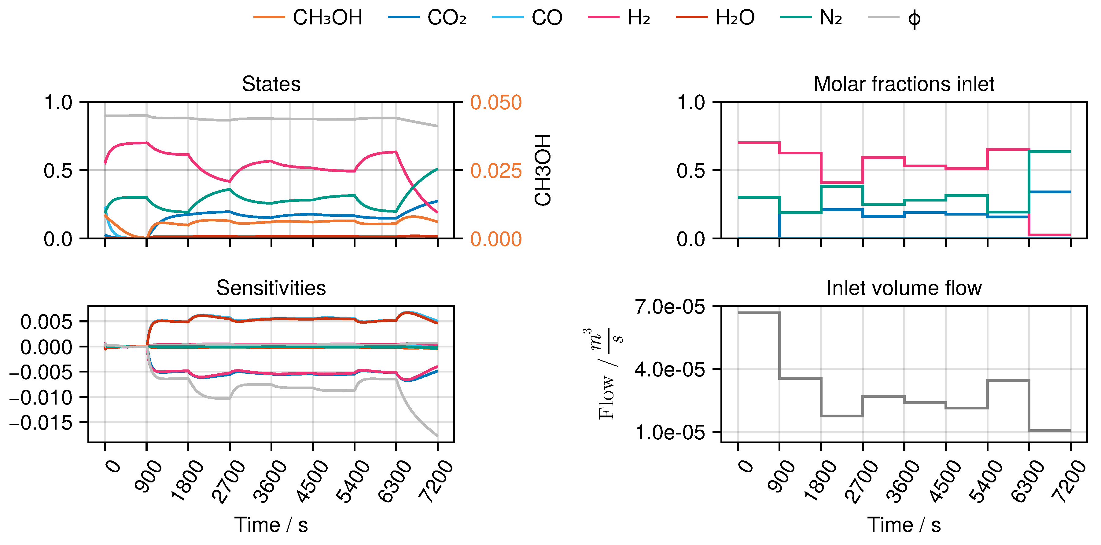
Figure A19.
As in Figure A16, but for the kinetic equation for the differential state . The temperature was determined as °C.
Figure A19.
As in Figure A16, but for the kinetic equation for the differential state . The temperature was determined as °C.
Appendix E.3. OED for Hybrid Model
After training the hybrid model on the collected experimental data, we computed an additional experimental design to collect insightful data for further training of the embedded neural network. We identified the most important weights and biases of the network by decomposing the Fisher information matrix in a singular value decomposition which we truncated to the two largest singular values. In contrast to the previous experimental designs, for this experiment we chose a discretization parameter of s, while the other options, bounds and initial values remained the same. The obtained solution is illustrated in Figure 7.
Appendix E.4. Graphical Comparison of Optimal and Heuristic Designs
We compare the exploration of the state space using optimal experimental design with the previously collected experiments using the relative density
over the training set. Here denotes a (data) bin centered at and is the indicator function which returns 1 if the point was generated using optimal experimental design.
Figure A20 shows the full set of states and controls of the reactor over all trajectories available. Table A10 shows the relative density for all pairs of variables corresponding to the data shown in Figure A20.
Figure A20.
Comparison of the relative state space exploration due to optimal experimental design. Each pair represents a two-dimensional slice of the full state space, the color indicates the ratio . The state space has been divided into 15 equidistant bins for each variable.
Figure A20.
Comparison of the relative state space exploration due to optimal experimental design. Each pair represents a two-dimensional slice of the full state space, the color indicates the ratio . The state space has been divided into 15 equidistant bins for each variable.
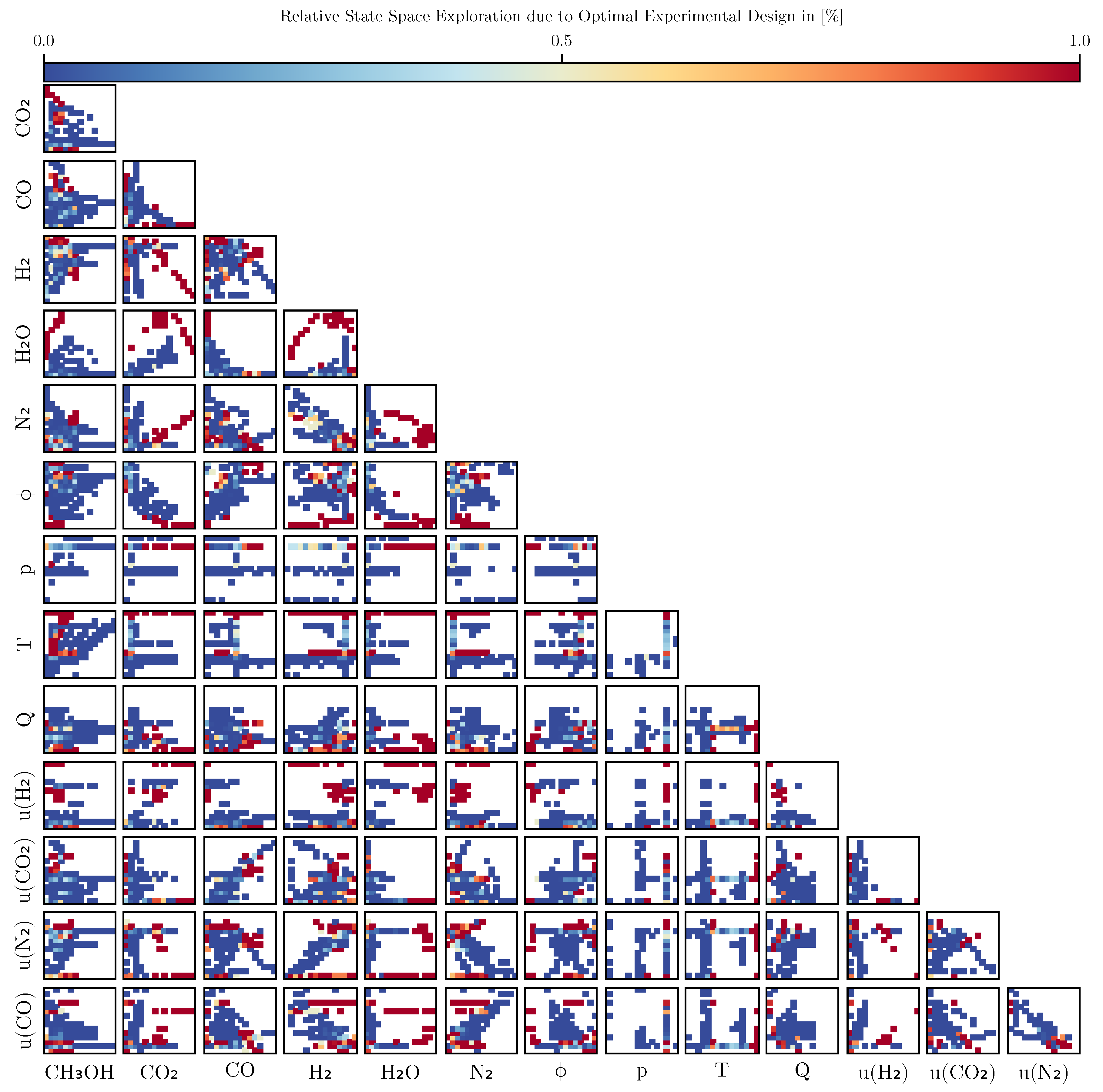
Table A10.
Relative density over two-dimensional sections of the entire state space and all related controls.
Table A10.
Relative density over two-dimensional sections of the entire state space and all related controls.
| CO | p | T | |||||||||||
|---|---|---|---|---|---|---|---|---|---|---|---|---|---|
| 0.247 | |||||||||||||
| CO | 0.146 | 0.286 | |||||||||||
| 0.245 | 0.415 | 0.292 | |||||||||||
| 0.219 | 0.399 | 0.225 | 0.523 | ||||||||||
| 0.205 | 0.357 | 0.291 | 0.272 | 0.487 | |||||||||
| 0.18 | 0.233 | 0.208 | 0.349 | 0.364 | 0.306 | ||||||||
| p | 0.0615 | 0.229 | 0.119 | 0.142 | 0.305 | 0.0964 | 0.127 | ||||||
| T | 0.252 | 0.267 | 0.234 | 0.333 | 0.364 | 0.287 | 0.219 | 0.154 | |||||
| 0.149 | 0.337 | 0.245 | 0.259 | 0.461 | 0.181 | 0.253 | 0.126 | 0.243 | |||||
| 0.294 | 0.366 | 0.198 | 0.47 | 0.468 | 0.44 | 0.223 | 0.239 | 0.281 | 0.281 | ||||
| 0.127 | 0.218 | 0.202 | 0.266 | 0.235 | 0.22 | 0.159 | 0.132 | 0.18 | 0.143 | 0.202 | |||
| 0.227 | 0.395 | 0.276 | 0.388 | 0.513 | 0.311 | 0.29 | 0.125 | 0.235 | 0.173 | 0.325 | 0.153 | ||
| 0.231 | 0.372 | 0.264 | 0.366 | 0.478 | 0.383 | 0.291 | 0.13 | 0.214 | 0.148 | 0.303 | 0.178 | 0.209 | |
| Mean | 0.199 | 0.323 | 0.232 | 0.337 | 0.408 | 0.278 | 0.223 | 0.151 | 0.231 | 0.186 | 0.277 | 0.166 | 0.209 |
References
- Olah, G.A.; Goeppert, A.; Prakash, G.S. Beyond oil and gas: the methanol economy; John Wiley & Sons, 2011. [Google Scholar]
- Keßler, T.; Plate, C.; Martensen, C.J.; Leipold, J.; Seidel-Morgenstern, A.; Sager, S.; Kienle, A. Two degress of freedom control of a multistage power to methanol reactor. Computers Chem. Eng. 2024, 192, 108893. [Google Scholar] [CrossRef]
- Wang, X.; Liu, Y.; Li, X.; Liu, D. Heterogeneous catalysts, reaction kinetics, and reactor designs for methanol production from carbon dioxide: A critical review. The Canadian Journal of Chemical Engineering 2024, 102, 1592–1629. [Google Scholar] [CrossRef]
- Beck, A.; Newton, M.A.; van de Water, L.G.; van Bokhoven, J.A. The Enigma of Methanol Synthesis by Cu/ZnO/Al2O3-Based Catalysts. Chemical Reviews 2024, 124, 4543–4678. [Google Scholar] [CrossRef] [PubMed]
- Seidel, C.; Jörke, A.; Vollbrecht, B.; Seidel-Morgenstern, A.; Kienle, A. Kinetic modeling of methanol synthesis from renewable resources. Chemical Engineering Science 2018, 175, 130–138. [Google Scholar] [CrossRef]
- Seidel, C.; Jörke, A.; Vollbrecht, B.; Seidel-Morgenstern, A.; Kienle, A. Corrigendum to’Kinetic modeling of methanol synthesis from renewable resources’(Chem. Eng. Sci. 175 (2018) 130-138). Chem. Eng. Sci 2020, 223, 115724. [Google Scholar] [CrossRef]
- Seidel, C.; Nikolić, D.; Felischak, M.; Petkovska, M.; Seidel-Morgenstern, A.; Kienle, A. Optimization of Methanol Synthesis under Forced Periodic Operation. Processes 2021, 9, 872. [Google Scholar] [CrossRef]
- Vollbrecht, B. Zur Kinetik der Methanolsynthese an einem technischen Cu/ZnO/Al2O3-Katalysator; Docupoint-Verlag, 2007. [Google Scholar]
- Rackauckas, C.; Ma, Y.; Martensen, J.; Warner, C.; Zubov, K.; Supekar, R.; Skinner, D.; Ramadhan, A.; Edelman, A. Universal Differential Equations for Scientific Machine Learning. arXiv 2021, arXiv:2001.04385. [Google Scholar] [CrossRef]
- Plate, C.; Martensen, C.J.; Sager, S. Optimal Experimental Design for Universal Differential Equations, 2024, [2408. arXiv 2024, arXiv:2408.07143. [Google Scholar] [CrossRef]
- Berty, J.M. Reactor for Vapor-Phase Catalytic Studies. Chemical Engineering Progress 1974, 70, 78–84. [Google Scholar]
- Handbook of Heterogeneous Catalysis: Online, 1st ed.; Ertl, G., Knözinger, H., Schüth, F., Weitkamp, J., Eds.; Wiley, 2008. [Google Scholar] [CrossRef]
- Fichtl, M.B.; Schlereth, D.; Jacobsen, N.; Kasatkin, I.; Schumann, J.; Behrens, M.; Schlögl, R.; Hinrichsen, O. Kinetics of deactivation on Cu/ZnO/Al2O3 methanol synthesis catalysts. Applied Catalysis A: General 2015, 502, 262–270. [Google Scholar] [CrossRef]
- Lunkenbein, T.; Girgsdies, F.; Kandemir, T.; Thomas, N.; Behrens, M.; Schlögl, R.; Frei, E. Bridging the Time Gap: A Copper/Zinc Oxide/Aluminum Oxide Catalyst for Methanol Synthesis Studied under Industrially Relevant Conditions and Time Scales. Angewandte Chemie International Edition 2016, 55, 12708–12712. [Google Scholar] [CrossRef] [PubMed]
- Sun, J.T.; Metcalfe, I.S.; Sahibzada, M. Deactivation of Cu/ZnO/Al2 O3 Methanol Synthesis Catalyst by Sintering. Industrial & Engineering Chemistry Research 1999, 38, 3868–3872. [Google Scholar] [CrossRef]
- Pinto, J.; Mestre, M.; Ramos, J.; Costa, R.S.; Striedner, G.; Oliveira, R. A general deep hybrid model for bioreactor systems: Combining first principles with deep neural networks. Computers & Chemical Engineering 2022, 165, 107952. [Google Scholar] [CrossRef]
- Schweidtmann, A.M.; Zhang, D.; Von Stosch, M. A review and perspective on hybrid modeling methodologies. Digital Chemical Engineering 2024, 10, 100136. [Google Scholar] [CrossRef]
- Martensen, C.J.; Plate, C.; Keßler, T.; Kunde, C.; Kaps, L.; Kienle, A.; Seidel-Morgenstern, A.; Sager, S. Towards Machine Learning of Power-2-Methanol Processes. In Computer Aided Chemical Engineering; Kokossis, A.C.; Georgiadis, M.C.; Pistikopoulos, E., Eds.; Elsevier, 2023; Vol. 52, 33 European Symposium on Computer Aided Process Engineering, pp. 561–568. [CrossRef]
- Bezanson, J.; Edelman, A.; Karpinski, S.; Shah, V.B. Julia: A Fresh Approach to Numerical Computing. SIAM Review 2017, 59, 65–98. [Google Scholar] [CrossRef]
- Dixit, V.K.; Rackauckas, C. Optimization.Jl: A Unified Optimization Package. Zenodo, 2023. [CrossRef]
- Nocedal, J.; Wright, S.J. Large-Scale Unconstrained Optimization. In Numerical Optimization. In Numerical Optimization; Springer: New York, NY, 2006; pp. 164–192. [Google Scholar] [CrossRef]
- Mogensen, P.K.; Riseth, A.N. Optim: A Mathematical Optimization Package for Julia. Journal of Open Source Software 2018, 3, 615. [Google Scholar] [CrossRef]
- Kingma, D.P.; Ba, J. Adam: A Method for Stochastic Optimization. arXiv 2017, arXiv:1412.6980. [Google Scholar] [CrossRef]
- Rätze, K.H.; Kortuz, W.; Kirschtowski, S.; Jokiel, M.; Hamel, C.; Sundmacher, K. Optimal experimental design for the identification of a reaction kinetic model for the hydroaminomethylation of 1-decene in a thermomorphic multiphase system. Chemical Engineering Journal 2023, 469, 143713. [Google Scholar] [CrossRef]
- Bubel, M.; Schmid, J.; Kozachynskyi, V.; Esche, E.; Bortz, M. Sequential optimal experimental design for vapor-liquid equilibrium modeling. arXiv 2024, arXiv:2403.09443. [Google Scholar] [CrossRef]
- Fedorov, V. Theory of optimal experiments; Academic Press: New York and London, 1972. [Google Scholar]
- Atkinson, A.; Donev, A. Optimum Experimental Designs; Number 8 in Oxford Statistical Sciences Series; Oxford University Press: Oxford, 1992. [Google Scholar]
- Pukelsheim, F. Optimal design of experiments; Wiley: New York, 1993. [Google Scholar]
- Kitsos, C. Optimal Experimental Design for Non-Linear Models; Springer: Heidelberg, 2013. [Google Scholar]
- Körkel, S. Numerische Methoden für Optimale Versuchsplanungsprobleme bei nichtlinearen DAE-Modellen. https://archiv.ub.uni-heidelberg.de/volltextserver/2980/, 2002. [CrossRef]
- Sager, S. Sampling Decisions in Optimum Experimental Design in the Light of Pontryagin’s Maximum Principle. SIAM Journal on Control and Optimization 2013, 51, 3181–3207. [Google Scholar] [CrossRef]
- Wächter, A.; Biegler, L.T. On the Implementation of an Interior-Point Filter Line-Search Algorithm for Large-Scale Nonlinear Programming. Mathematical Programming 2006, 106, 25–57. [Google Scholar] [CrossRef]
- Lundberg, S.M.; Lee, S.I. A Unified Approach to Interpreting Model Predictions. In Proceedings of the Proceedings of the 31st International Conference on Neural Information Processing Systems, Red Hook, NY, USA, 2017.
- Quaghebeur, W.; Torfs, E.; Khalil, M.; Nopens, I.; De Baets, B. Uncovering Unknown Dynamics in Water Resource Recovery Facilities with Neural Differential Equations and Shapley Value Analysis. Journal of Water Process Engineering 2025, 70, 106856. [Google Scholar] [CrossRef]
- Schwaab, M.; Pinto, J.C. Optimum reference temperature for reparameterization of the Arrhenius equation. Part 1: Problems involving one kinetic constant. Chemical Engineering Science 2007, 62, 2750–2764. [Google Scholar] [CrossRef]
- Schwaab, M.; Lemos, L.P.; Pinto, J.C. Optimum reference temperature for reparameterization of the Arrhenius equation. Part 2: Problems involving multiple reparameterizations. Chemical Engineering Science 2008, 63, 2895–2906. [Google Scholar] [CrossRef]
- Skrzypek, J.; Słoczyński, J.; Ledakowicz, S. Methanol synthesis: science and engineering; Polish Scientific Publ: Warszawa, 1994. [Google Scholar]
| 1 | Full code and versioning of all related software is available at https://kosinus.math.uni-magdeburg.de/AlCap23/berty-parameter-estimation
|
Figure 1.
Reaction network of methanol synthesis showing the different pathways and their respective reaction rates, which depend on the current state of the catalyst.
Figure 1.
Reaction network of methanol synthesis showing the different pathways and their respective reaction rates, which depend on the current state of the catalyst.
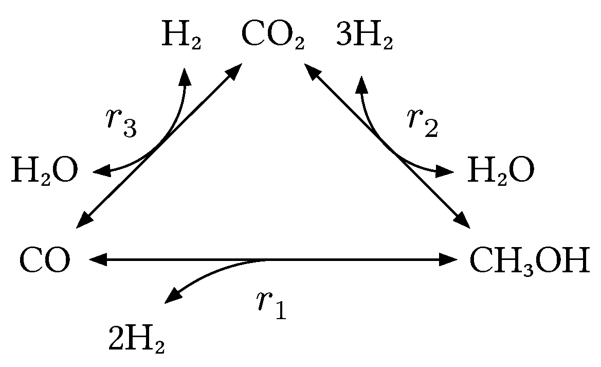
Figure 2.
Scheme of experimental set-up: gas supply from gas bottles via mass flow controllers (MFC’s), Berty type reactor filled with CuO/ZnO/Al2O3 catalyst and analytics (µ-gas chromatography from Agilent). The reactor is monitored and controlled for temperature and pressure. The latter is regulated via a membrane back pressure regulator. Further on the downstream side the pressure is released through a relief valve to 4 bar, ensuring a continuous effluent flow. In order to protect the electric engine of the stirrer from the reaction media and heat, N2 is flushed from the top into the reaction chamber. N2 is used also as an indicator component to quantify the volume contraction caused by the reactions.
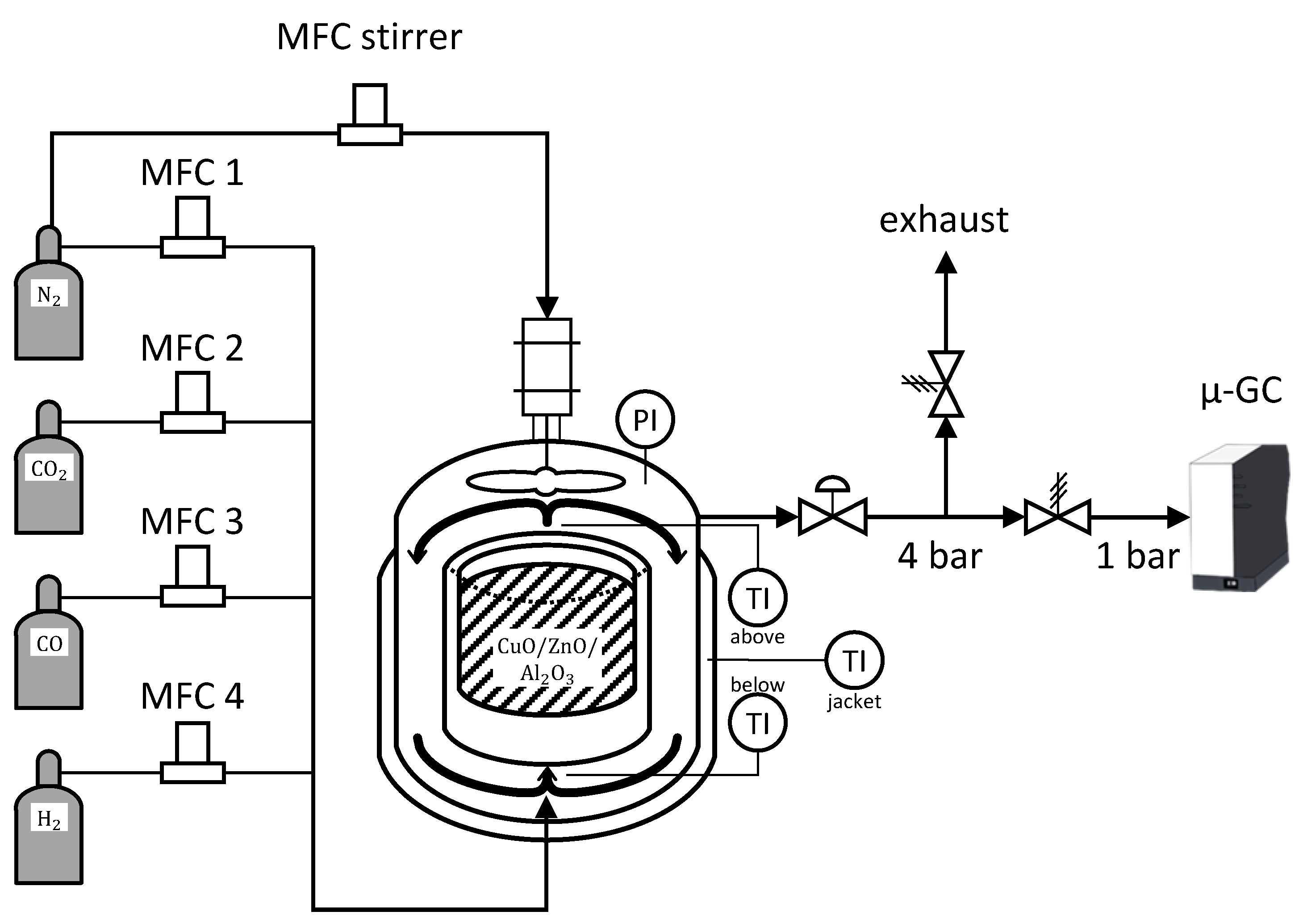
Figure 3.
Example of a single experiment (MeOH_028). Top Measured output of the reactor as mole fractions. Middle Feed composition to the reactor as mole fractions and total volumetric flow rate. Bottom Temperature and pressure of the reactor.
Figure 3.
Example of a single experiment (MeOH_028). Top Measured output of the reactor as mole fractions. Middle Feed composition to the reactor as mole fractions and total volumetric flow rate. Bottom Temperature and pressure of the reactor.
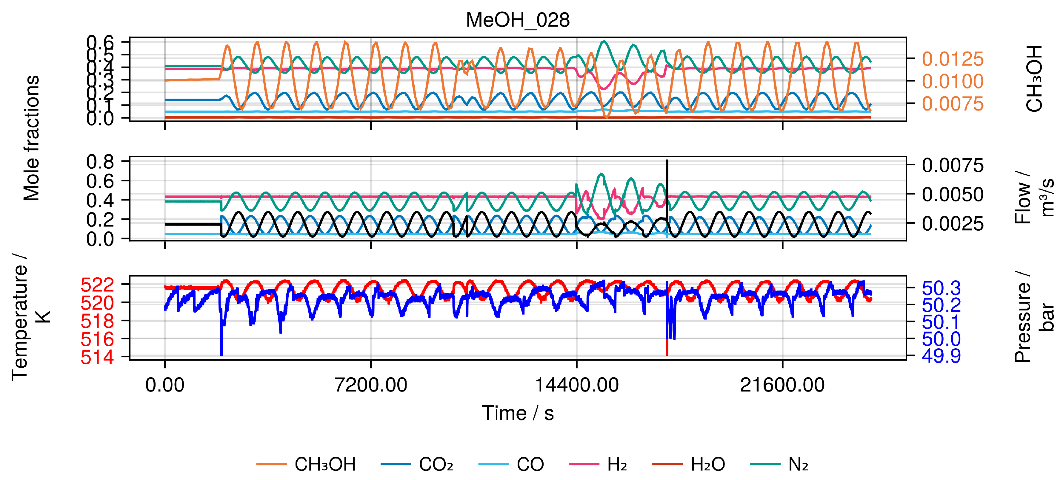
Figure 4.
Block diagram of the mechanistic model in the form of a DAE system. Our goal is to learn the impact of the catalyst state on the reaction rates r directly from the data. The triangle ▵ denotes concatenation, ⊙ denotes elementwise multiplication.
Figure 4.
Block diagram of the mechanistic model in the form of a DAE system. Our goal is to learn the impact of the catalyst state on the reaction rates r directly from the data. The triangle ▵ denotes concatenation, ⊙ denotes elementwise multiplication.
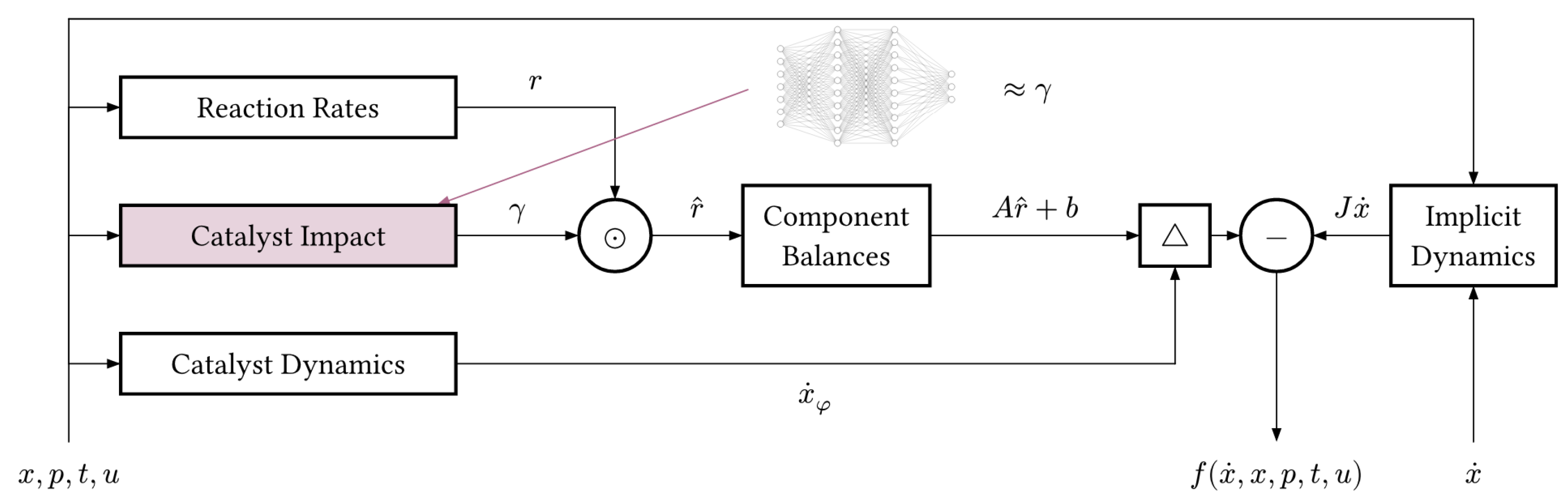
Figure 5.
Parity plot of the fitted mechanistic model over the test data set. The color of each species matches the trajectory plots.
Figure 5.
Parity plot of the fitted mechanistic model over the test data set. The color of each species matches the trajectory plots.
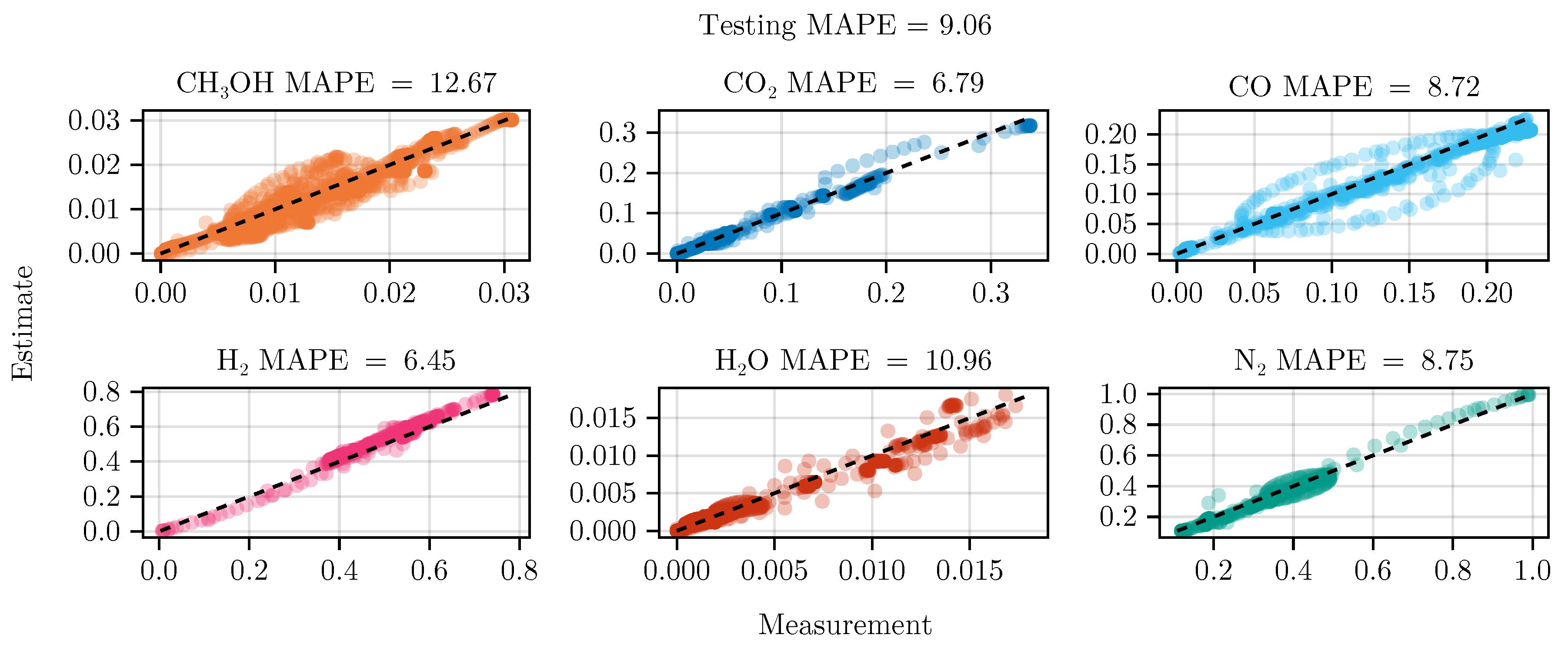
Figure 6.
Model prediction on the experiment MeOH_079. After the initial catalyst activity was determined at the reference condition the reactor was heated up. The temperature and the following six feed compositions and flow rates, each applied for 20 min, were chosen randomly within relevant process boundaries. Top The state trajectory. Colored scatter denotes the data, full lines the prediction. Middle The feed of the reactor in mole fractions using the respective color for each species. The black line denotes the incoming volumetric flow rate. Bottom The temperature (red) and pressure (blue) over the time course of the experiment.
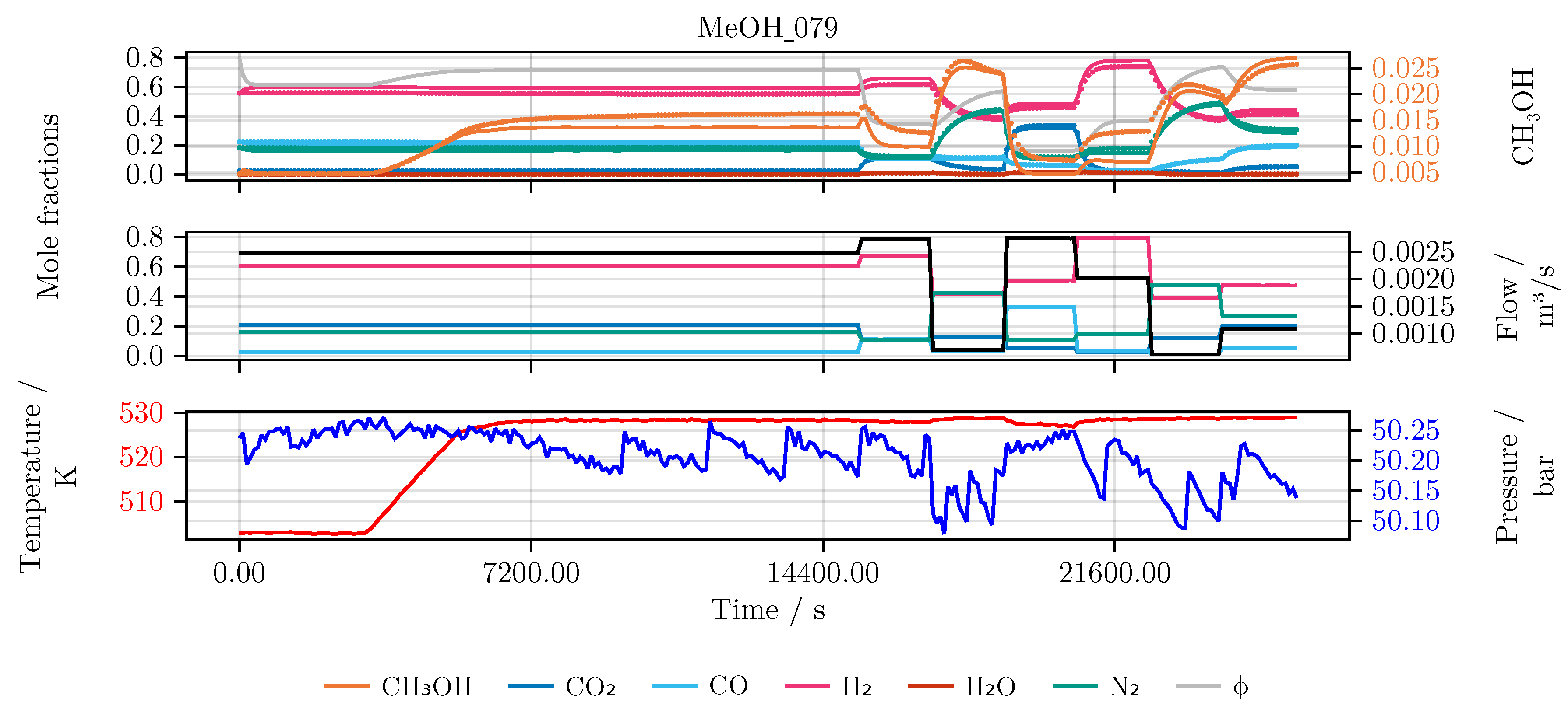
Figure 7.
Optimal experimental design MeOH_083 of the selected architecture B. The temperature was determined as K.
Figure 7.
Optimal experimental design MeOH_083 of the selected architecture B. The temperature was determined as K.
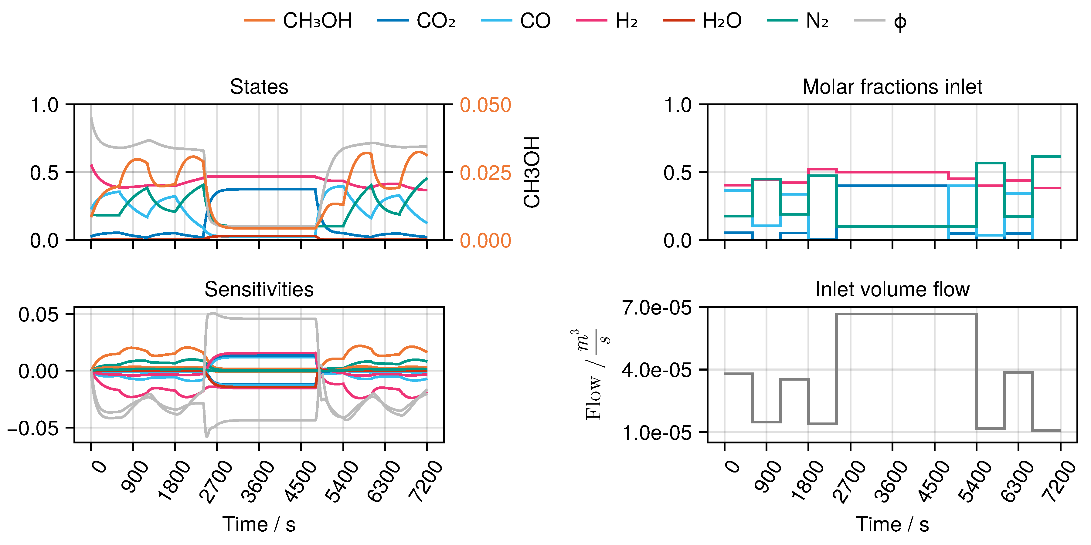
Figure 8.
Parity plot of the fitted hybrid model over the train data set. The color of each species matches the trajectory plots.
Figure 8.
Parity plot of the fitted hybrid model over the train data set. The color of each species matches the trajectory plots.
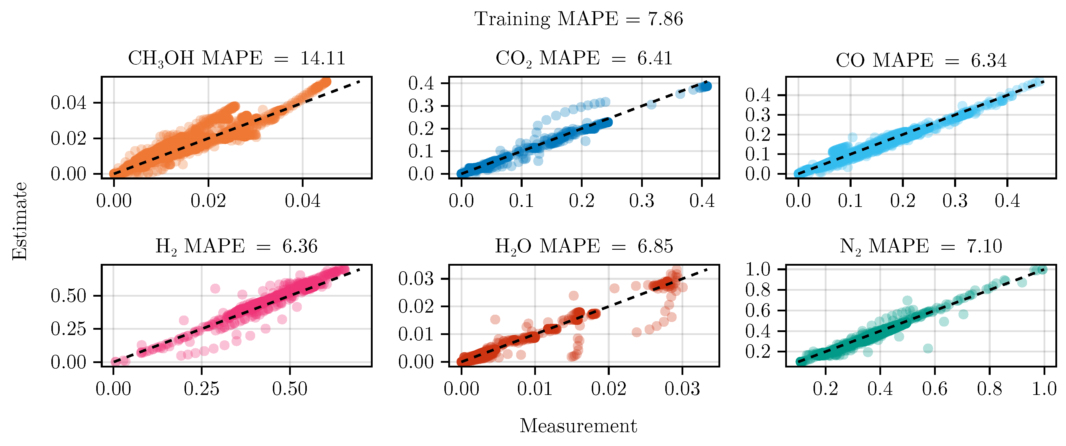
Figure 9.
Parity plot comparing the functional relationship of the trained neural network and the previous heuristic for the impacts Equation 10 evaluated on the train dataset. While the neural network and the heuristic deviate for , there is a high level of agreement for both and . The visible mismatch for RWGS stems from only the top 3% of data. Note The mean absolute percentage error does not indicate a goodness-of-fit in this case, but rather the divergence between the heuristic and the ML model.
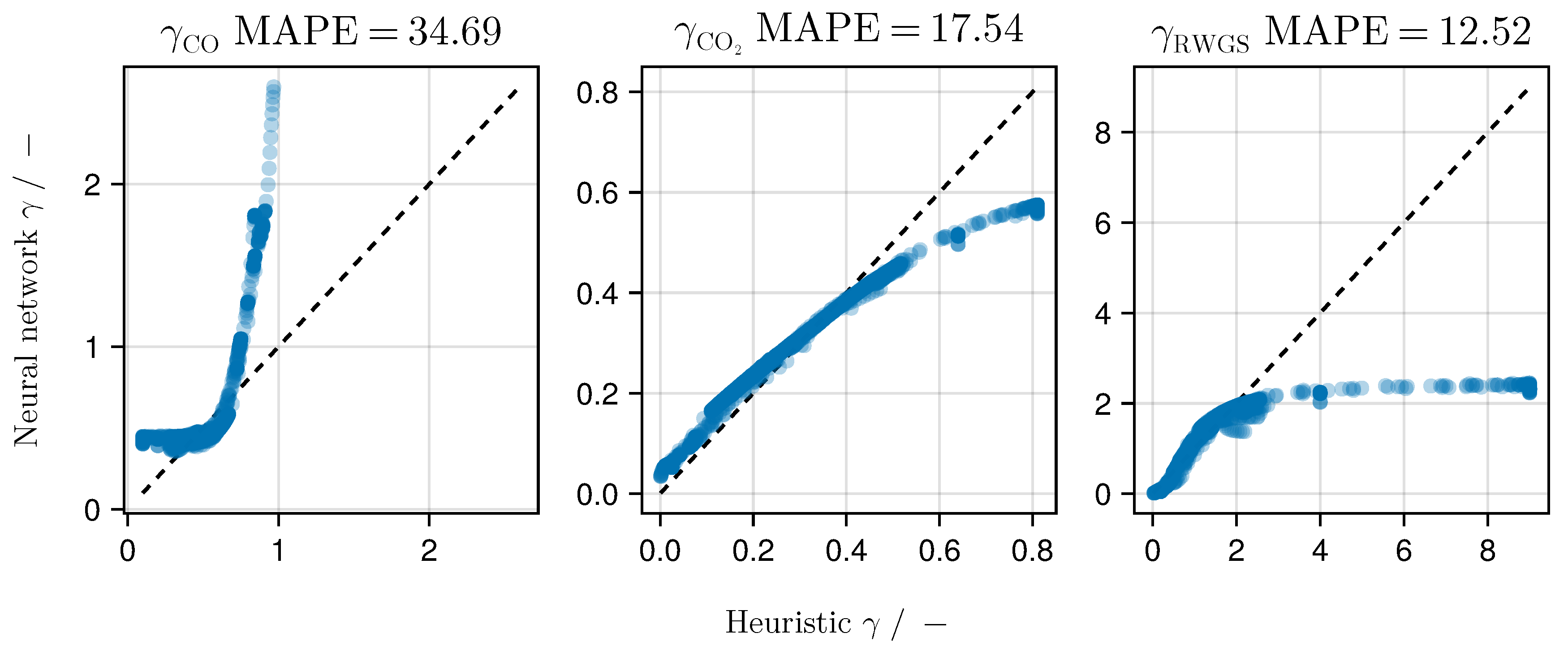
Figure 10.
Comparison of heuristic and optimal experimental designs over the prediction of the final, fully trained mechanistic model. The color indicates the relative density of points in a bin due to optimal experimental design. See Section Appendix E.4 for a more detailed explanation.
Figure 10.
Comparison of heuristic and optimal experimental designs over the prediction of the final, fully trained mechanistic model. The color indicates the relative density of points in a bin due to optimal experimental design. See Section Appendix E.4 for a more detailed explanation.
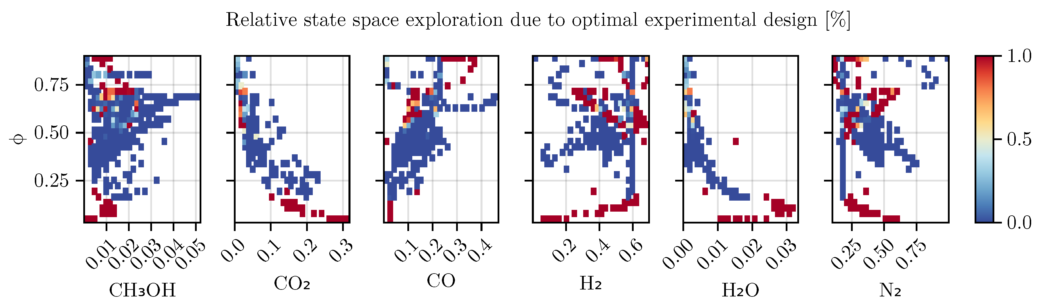
Table 1.
Hyperparameters for initial training of hybrid model. The function swish is given by , denotes the typical sigmoid function .
Table 1.
Hyperparameters for initial training of hybrid model. The function swish is given by , denotes the typical sigmoid function .
| Hyperparameter | Hidden Layers | Layer Width | Activation |
|---|---|---|---|
| Options | 2, 3, 4 | 5, 10, 15 |
Table 2.
Lower and upper bounds on control functions and control values for the optimal experimental design.
Table 2.
Lower and upper bounds on control functions and control values for the optimal experimental design.
| Variable | Lower Bound | Upper Bound | Unit |
|---|---|---|---|
| T | 500.0 | 530.0 | K |
| 0.5 | 4.0 | Ln / min | |
| 0.0 | 40.0 | % | |
| 0.0 | 40.0 | % | |
| 0.0 | 75.0 | % | |
| 0.0 | 100.0 | % |
Table 3.
Initial conditions assumed in all OED problems.
| State | Initial value |
|---|---|
| 0.00854 | |
| 0.02494 | |
| 0.22906 | |
| 0.55062 | |
| 0.00184 | |
| 0.18499 | |
| 0.7 |
Table 4.
Results of the different model architectures and fitting procedure. We report the mean absolute percentage error MAPE = for the respective dataset and species ( denotes the states). (OED) indiciates the use of the full training data including the data from the optimal experimental designs, (NOED) the use of the dataset without optimal designs. The hybrid model (INIT) denotes the best architecture after hyperoptimization and subsequent fit using L-BFGS. The best value of each column is bold.
| MAPE | |||||||
|---|---|---|---|---|---|---|---|
| State | Total | ||||||
| Train | |||||||
| Mechanistic (OED) | 13.60 | 6.89 | 6.41 | 6.42 | 6.89 | 7.15 | 7.90 |
| Mechanistic (NOED) | 25.20 | 6.69 | 5.79 | 6.57 | 16.10 | 7.27 | 11.30 |
| Hybrid Model (INIT) | 14.80 | 7.22 | 6.72 | 6.46 | 9.25 | 7.19 | 8.61 |
| Hybrid Model (NOED) | 32.90 | 5.96 | 7.19 | 7.01 | 16.40 | 7.70 | 12.90 |
| Hybrid Model (OED) | 14.10 | 6.34 | 6.41 | 6.36 | 6.85 | 7.10 | 7.86 |
| Test | |||||||
| Mechanistic (OED) | 12.70 | 8.72 | 6.79 | 6.45 | 11.00 | 8.75 | 9.06 |
| Mechanistic (NOED) | 32.90 | 10.10 | 6.43 | 6.56 | 14.50 | 8.96 | 13.20 |
| Hybrid Model (INIT) | 16.00 | 9.15 | 6.96 | 6.52 | 12.90 | 8.81 | 10.00 |
| Hybrid Model (NOED) | 24.10 | 8.83 | 6.96 | 6.73 | 12.10 | 8.99 | 11.30 |
| Hybrid Model (OED) | 10.00 | 9.05 | 6.68 | 6.33 | 10.20 | 8.65 | 8.49 |
Table 5.
Top 5 results of the hyperparameter search, their respective architecture and performance on the training set in terms of the coefficient of determination. Note we initially used the coefficient of determination instead of the MAPE for model selection. Hence, we report these values here. See Section Appendix D for a more detailed explanation.
| State | Total | ||||||
|---|---|---|---|---|---|---|---|
| Architecture | |||||||
| A 2 layer, 5 neurons, | 0.405 | 0.973 | 0.963 | 0.802 | -0.175 | 0.966 | 0.927 |
| 4 layer, 5 neurons, | 0.500 | 0.974 | 0.962 | 0.796 | -0.010 | 0.966 | 0.925 |
| 4 layer, 5 neurons, | 0.522 | 0.976 | 0.966 | 0.785 | 0.305 | 0.964 | 0.923 |
| 4 layer, 5 neurons, | 0.440 | 0.975 | 0.966 | 0.774 | 0.097 | 0.963 | 0.919 |
| B 2 layer, 5 neurons, swish | 0.476 | 0.978 | 0.969 | 0.772 | 0.556 | 0.961 | 0.919 |
Table 6.
Mean absolute Shapley values and their standard deviations for the input features of the neural network A evaluated on the training set computed via the implementation in Shapley.jl. A higher value indicates a stronger influence. Similar to the previously used heuristic, the neural net bases its decision primarily on the state .
| Mean absolute Shapley effect and standard deviation | |||
|---|---|---|---|
| State | |||
| 2.99e-04 ± 4.36e-04 | 8.00e-05 ± 1.23e-04 | 4.75e-04 ± 6.72e-04 | |
| 2.94e-03 ± 8.09e-03 | 3.63e-03 ± 6.13e-03 | 2.25e-02 ± 3.85e-02 | |
| 1.29e-03 ± 3.15e-03 | 6.07e-04 ± 8.40e-04 | 4.09e-03 ± 5.46e-03 | |
| 1.01e-02 ± 1.23e-02 | 6.30e-04 ± 1.25e-03 | 4.94e-02 ± 5.87e-02 | |
| 2.67e-04 ± 8.11e-04 | 1.15e-05 ± 1.66e-05 | 3.55e-05 ± 8.03e-05 | |
| 1.04e-02 ± 1.56e-02 | 2.72e-03 ± 3.18e-03 | 1.06e-02 ± 1.27e-02 | |
| 8.30e-02 ± 1.83e-01 | 8.84e-02 ± 1.04e-01 | 4.44e-01 ± 5.21e-01 | |
Disclaimer/Publisher’s Note: The statements, opinions and data contained in all publications are solely those of the individual author(s) and contributor(s) and not of MDPI and/or the editor(s). MDPI and/or the editor(s) disclaim responsibility for any injury to people or property resulting from any ideas, methods, instructions or products referred to in the content. |
© 2025 by the authors. Licensee MDPI, Basel, Switzerland. This article is an open access article distributed under the terms and conditions of the Creative Commons Attribution (CC BY) license (http://creativecommons.org/licenses/by/4.0/).
Copyright: This open access article is published under a Creative Commons CC BY 4.0 license, which permit the free download, distribution, and reuse, provided that the author and preprint are cited in any reuse.


