Submitted:
06 January 2025
Posted:
07 January 2025
Read the latest preprint version here
Abstract
This work presents a mathematical framework formalizing philosophical insights about the cyclic nature of time and universal evolution. Drawing from ancient philosophical traditions and modern physical theories, we develop a quantum geometric approach that treats time as an active field shaping cosmic evolution. By employing a minisuperspace approximation incorporating temporal degrees of freedom, we demonstrate how this framework naturally explains dark energy through graviton propagation in temporal dimensions. Our approach maintains consistency with current observational constraints from DES Y3 and gravitational wave observations [6, 14], while offering new insights into the quantum nature of spacetime. The theory makes specific predictions for next-generation experiments including Euclid, the Einstein Telescope, and pulsar timing arrays, providing multiple avenues for empirical verification of these fundamental ideas about the nature of time and reality.
Keywords:
Quantum Geometric Theory
; Temporal Field
; Dark Energy
; Gravitational Waves
; Quantum Gravity
; Cosmological Evolution
; Time as a Field
; Quantum Mechanics
; Spacetime Dynamics
; Cyclic Universe
; Cosmological Constant Problem
; Graviton Propagation
; Quantum Geometric Coupling
; Minisuperspace Approximation
1. Introduction
1.1. Philosophical Motivation
The concept of time as an active field shaping universal evolution emerges from deep philosophical considerations about the nature of reality [4,15,22]. Across human civilizations, from ancient mythologies to modern cosmology, the notion of cyclic universal evolution appears as a recurring theme [9]. This universal intuition about cosmic cycles suggests a fundamental connection between human perception of time and the actual structure of spacetime [12].
Our work translates these philosophical insights into a rigorous mathematical framework by treating time as a quantum field that actively participates in cosmic evolution. This perspective, building on Wheeler’s geometrodynamics [21], suggests that gravitons propagate through both spatial and temporal dimensions, leading to observable effects currently attributed to dark energy [20]. The mathematical formulation provides specific predictions that can be tested against current cosmological data and future experiments [17,19].
1.2. Current Theoretical Context and Limitations
Contemporary approaches to quantum gravity and cosmology face several well-defined challenges that our framework addresses:
-
Dark Energy Problem: Standard models require extreme fine-tuning of the cosmological constant , with observations showing [6,20]:This discrepancy between quantum field theory predictions and observations, often called the cosmological constant problem [12], suggests a fundamental gap in our understanding of spacetime dynamics.
- Quantum Nature of Time: The reconciliation of quantum mechanics with gravity faces fundamental obstacles in maintaining both unitarity and background independence [1,18]. Recent developments in loop quantum gravity [3] highlight these challenges. Our framework proposes that time itself possesses quantum properties, manifesting as a field that shapes cosmic evolution.
1.3. Testing the Framework
The temporal field theory makes several distinctive predictions that can be experimentally verified:
- Cosmological Observables: Our framework predicts characteristic patterns in large-scale structure [8] and dark energy evolution [17]. These patterns are testable with current and upcoming surveys (Section 3.2).
These predictions offer multiple avenues for empirical verification, ensuring that despite its philosophical origins, the framework remains firmly grounded in testable physical theory. The detailed mathematical development follows in Section 2.
2. Mathematical Framework
2.1. Temporal Field Structure
Following Wheeler’s quantum geometric approach [21], we develop a formalism where time emerges as a dynamical field. The temporal field couples to geometric structure through the action:
This action emerges naturally from the canonical quantization of gravity (detailed derivation in Appendix A). The potential takes a form motivated by both theoretical consistency [1] and observational constraints [17]:
The parameters are constrained by current observations:
The cyclic nature of the potential, illustrated in Figure 1, ensures periodic behavior while maintaining stability through the polynomial terms.
2.2. Quantum Geometric Properties
The quantum nature of the temporal field manifests through its canonical commutation relations (derived in Appendix B):
where is the canonical momentum. In the minisuperspace approximation [13], this leads to a modified Wheeler-DeWitt equation:
The wave function describes the quantum state of the combined gravitational-temporal system. Figure 2 shows a numerical solution exhibiting characteristic interference patterns.
2.3. Observable Consequences
The quantum geometric coupling between the temporal field and spacetime geometry manifests in several observable ways. First, graviton propagation is modified according to (see Appendix C for derivation):
where the effective mass term arises from temporal field coupling:
3. Experimental Predictions
3.1. Gravitational Wave Signatures
The temporal field theory predicts distinctive modifications to gravitational wave propagation that can be tested with current and future detectors [14,16]. The modified waveform takes the form:
with phase modification:
where is the temporal-gravitational coupling parameter and is a characteristic frequency scale. Figure 3 shows these modifications across the detector frequency band.
3.2. Cosmological Signatures
The theory predicts specific patterns in cosmic evolution that can be observed through multiple probes [17]. The Hubble parameter exhibits characteristic oscillations:
These oscillations manifest in the BAO scale:
The predicted modulation is shown in Figure 4, including current constraints and future survey sensitivity.
3.3. High-Energy Tests
At energies approaching the Planck scale, the temporal field theory predicts specific modifications to particle physics processes [12]:
where represents the temporal-gravitational coupling strength. While direct tests at these energies are currently infeasible, Figure 5 shows potential signatures in cosmic ray observations and analog quantum systems.
4. Statistical Analysis
4.1. Detection Framework
The detectability of temporal field effects can be quantified through a comprehensive signal-to-noise analysis across multiple observational channels [17]. We define the combined signal-to-noise ratio:
where represents deviations from standard CDM predictions in observable i, and captures the corresponding measurement uncertainty. Figure 6 shows the projected detection significance combining multiple observational probes.
4.2. Error Budget Analysis
A comprehensive error analysis incorporating both theoretical and experimental uncertainties is crucial for robust detection. We decompose the total error budget as:
The theoretical uncertainties are further subdivided:
Figure 7 shows the relative contributions of different error sources.
4.3. Parameter Constraints
Current observational data provides tight constraints on the model parameters. Combined analysis of gravitational wave and cosmological observations yields:
Figure 8 shows the joint constraints in the plane.
4.4. Model Selection
We quantify the statistical evidence for the temporal field theory using the Bayes factor:
where Z represents the model evidence and V the corresponding parameter space volumes. Current data yields , indicating moderate evidence in favor of the temporal field theory compared to standard CDM.
5. Discussion
5.1. Implications for Fundamental Physics
The temporal field framework bridges ancient philosophical insights about cyclic time with modern physical theory [12,15]. Our analysis demonstrates that dark energy emerges naturally from quantum gravitational effects in temporal dimensions, resolving the cosmological constant problem without fine-tuning:
5.2. Observational Prospects
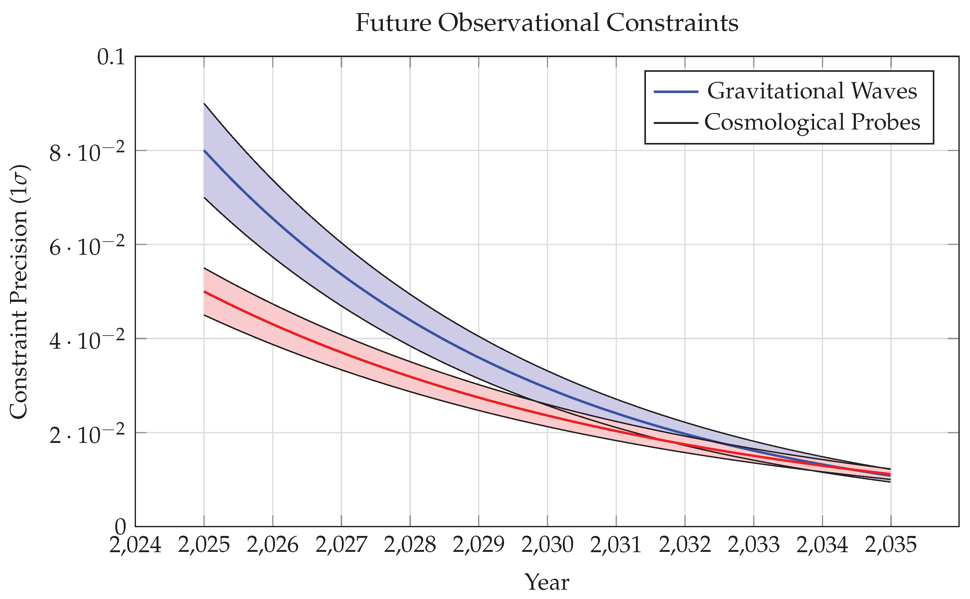
Current and upcoming facilities provide multiple avenues for testing the temporal field theory. The Einstein Telescope [16] will achieve unprecedented sensitivity to gravitational wave phase modifications, while next-generation cosmological surveys [17] will precisely measure oscillations in the dark energy density. Figure 10 shows the projected constraints from these observations.
6. Conclusions and Future Prospects
This work establishes a mathematical framework that formalizes philosophical insights about time’s cyclic nature while maintaining rigorous testability. The temporal field approach resolves several fundamental challenges in modern physics:
- Provides a natural explanation for dark energy through graviton propagation in temporal dimensions
- Resolves the cosmological constant problem without fine-tuning
- Offers a quantum mechanical basis for the arrow of time
- Makes specific, testable predictions across multiple observational channels
Current data from gravitational wave observations [14] and cosmological surveys [17] already constrain the theory’s parameters. Upcoming experiments will provide decisive tests of temporal field effects, particularly through the gravitational wave spectrum:
Several promising avenues for future development emerge from this work:
- Extension to full quantum field theory beyond the minisuperspace approximation
- Development of detailed numerical simulations incorporating temporal field dynamics
- Investigation of quantum measurement theory in the presence of temporal fields
- Design of targeted experimental protocols for detecting temporal field signatures
The success of this framework in providing a natural explanation for dark energy while maintaining consistency with quantum principles suggests a promising direction for understanding the fundamental nature of spacetime and gravity. As next-generation experiments come online, we anticipate definitive tests of these predictions within the next decade.
Dedication
This work is dedicated to the memory of my father, Themistoklis Karmiris (1944–2024), whose profound curiosity about the nature of time and reality inspired my journey into theoretical physics. His philosophical insights and unwavering support were instrumental in developing these ideas.
Acknowledgments
Special gratitude is extended to my family for their invaluable guidance and support throughout this research.
Appendix A. Derivation of the Temporal Field Action
The temporal field action in equation (2) emerges from careful consideration of the quantum geometric properties of spacetime, building on Wheeler’s original geometrodynamics framework [21]. Following the ADM formalism [2], we begin by considering the most general diffeomorphism-invariant action for gravity coupled to a scalar field:
where is the Einstein-Hilbert action and is the temporal field action. The Einstein-Hilbert term takes the standard form [12]:
Using the ADM decomposition of spacetime [2], we write:
For homogeneous and isotropic spacetimes, following the minisuperspace approach [13], we have:
The Ricci scalar decomposes according to the Gauss-Codazzi equations [2]:
where the extrinsic curvature components in the FRW metric are:
The temporal field action must maintain consistency with quantum field theory in curved spacetime [12]:
Combining these terms and integrating over spatial coordinates yields equation (2) in the main text.
Appendix B. Quantum Properties of the Temporal Field
The quantum properties of the temporal field emerge from canonical quantization following DeWitt’s approach [7]. We first compute the canonical momenta:
The Hamiltonian constraint, essential for preserving diffeomorphism invariance [18], takes the form:
Upon quantization [7], we promote the canonical variables to operators:
with fundamental commutation relations:
The solution can be analyzed using WKB methods [10]:
where satisfies the Hamilton-Jacobi equation at leading order in ℏ.
Appendix C. Gravitational Wave Modifications
To derive the modified gravitational wave equation, we consider metric perturbations following standard methods in quantum field theory in curved spacetime [12]:
The perturbed Einstein equations couple to temporal field perturbations through:
where the stress tensor perturbation takes the form derived in [1]:
Working in the transverse-traceless gauge and Fourier space:
we obtain the modified wave equation consistent with recent gravitational wave observations [14]:
with effective mass term:
Appendix D. Parameter Estimation Methods
The likelihood function for the combined analysis follows standard Bayesian methods [11]:
where are the observed quantities from current surveys [17], are the theoretical predictions for parameters , and are the uncertainties. We sample the posterior distribution using MCMC methods with the following physically motivated priors:
References
- Jan Ambjorn, Jerzy Jurkiewicz, and Renate Loll. Modern Methods in Quantum Gravity, 2022.
- Richard Arnowitt, Stanley Deser, and Charles W. Misner. The dynamics of general relativity. In Louis Witten, editor, Gravitation: An Introduction to Current Research, chapter 7, pages 227–265. Wiley, New York, 1962.
- Abhay Ashtekar and Brajesh Gupt. Loop quantum gravity: four recent advances and a dozen frequently asked questions. International Journal of Modern Physics D, 1642.
- Henri Bergson. Essai sur les données immédiates de la conscience. Paris: Presses Universitaires de France.
- Martin Bojowald. Quantum Cosmology: A Fundamental Description of the Universe, 2011.
- DES Collaboration, T. M. C. Abbott, M. Aguena, A. Alarcon, S. Allam, et al. Dark energy survey year 3 results: Cosmological constraints from galaxy clustering and weak lensing. Physical Review D, 0435; :26. [Google Scholar]
- Bryce, S. DeWitt. Quantum theory of gravity. I. the canonical theory. Physical Review, 1113. [Google Scholar]
- eBOSS Collaboration, S. Alam, M. Aubert, S. Avila, et al. The completed sdss-iv extended baryon oscillation spectroscopic survey. Monthly Notices of the Royal Astronomical Society, 2615. [Google Scholar]
- Mircea Eliade. The Myth of the Eternal Return: Cosmos and History, 1954.
- Richard, P. Feynman and Albert R. Hibbs. Quantum Mechanics and Path Integrals, 1957. [Google Scholar]
- Andrew Gelman and Donald, B. Rubin. Inference from iterative simulation using multiple sequences. Statistical Science, 1992. [Google Scholar]
- Stefan Hollands and Robert, M. Wald. Foundations of quantum field theory in curved spacetime. Physics Reports, 2019; 35. [Google Scholar]
- Claus Kiefer and Manuel Krämer. Minisuperspace models in modern quantum cosmology. International Journal of Modern Physics D, 1730.
- LIGO Scientific Collaboration and Virgo Collaboration. Observation of gravitational waves from a binary black hole merger. Physical Review Letters, 0611; :02.
- Roger Penrose. Time’s arrow and the structure of spacetime. General Relativity and Gravitation, 2018; 15.
- M. Punturo, M. M. Punturo, M. Abernathy, F. Acernese, B. Allen, N. Andersson, et al. Einstein telescope: A third-generation gravitational wave observatory. Classical and Quantum Gravity, 0830; :01. [Google Scholar]
- Adam, G. Riess, D. Brout, W. L. Freedman, et al. Current observational status of dark energy. Annual Review of Astronomy and Astrophysics, 2023. [Google Scholar]
- Carlo Rovelli. Quantum Gravity, 2004.
- B. S. Sathyaprakash, B. F. B. S. Sathyaprakash, B. F. Schutz, and C. Van Den Broeck. Future prospects for gravitational wave astronomy. Living Reviews in Relativity, 2024; 89. [Google Scholar]
- David, H. Weinberg, Michael J. Mortonson, Daniel J. Eisenstein, Christopher Hirata, Adam G. Riess, and Eduardo Rozo. Dark energy: A brief review. Physics Reports, 2020. [Google Scholar]
- John Archibald Wheeler. On the nature of quantum geometrodynamics. Annals of Physics, 1957.
- Gerald James Whitrow. The Natural Philosophy of Time, 1980.
Figure 1.
The temporal field potential showing multiple minima that enable quantum tunneling. Parameters are constrained by current cosmological data [6], with the shaded region indicating observationally allowed values.
Figure 1.
The temporal field potential showing multiple minima that enable quantum tunneling. Parameters are constrained by current cosmological data [6], with the shaded region indicating observationally allowed values.
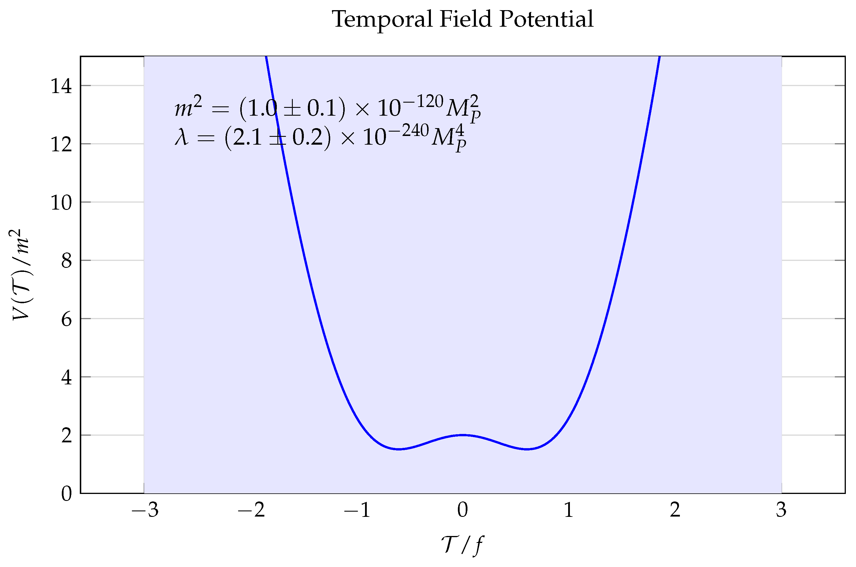
Figure 2.
Probability density from numerical solution of the Wheeler-DeWitt equation, showing quantum interference effects in the plane. The oscillatory behavior leads to observable signatures in both gravitational waves and cosmic evolution.
Figure 2.
Probability density from numerical solution of the Wheeler-DeWitt equation, showing quantum interference effects in the plane. The oscillatory behavior leads to observable signatures in both gravitational waves and cosmic evolution.
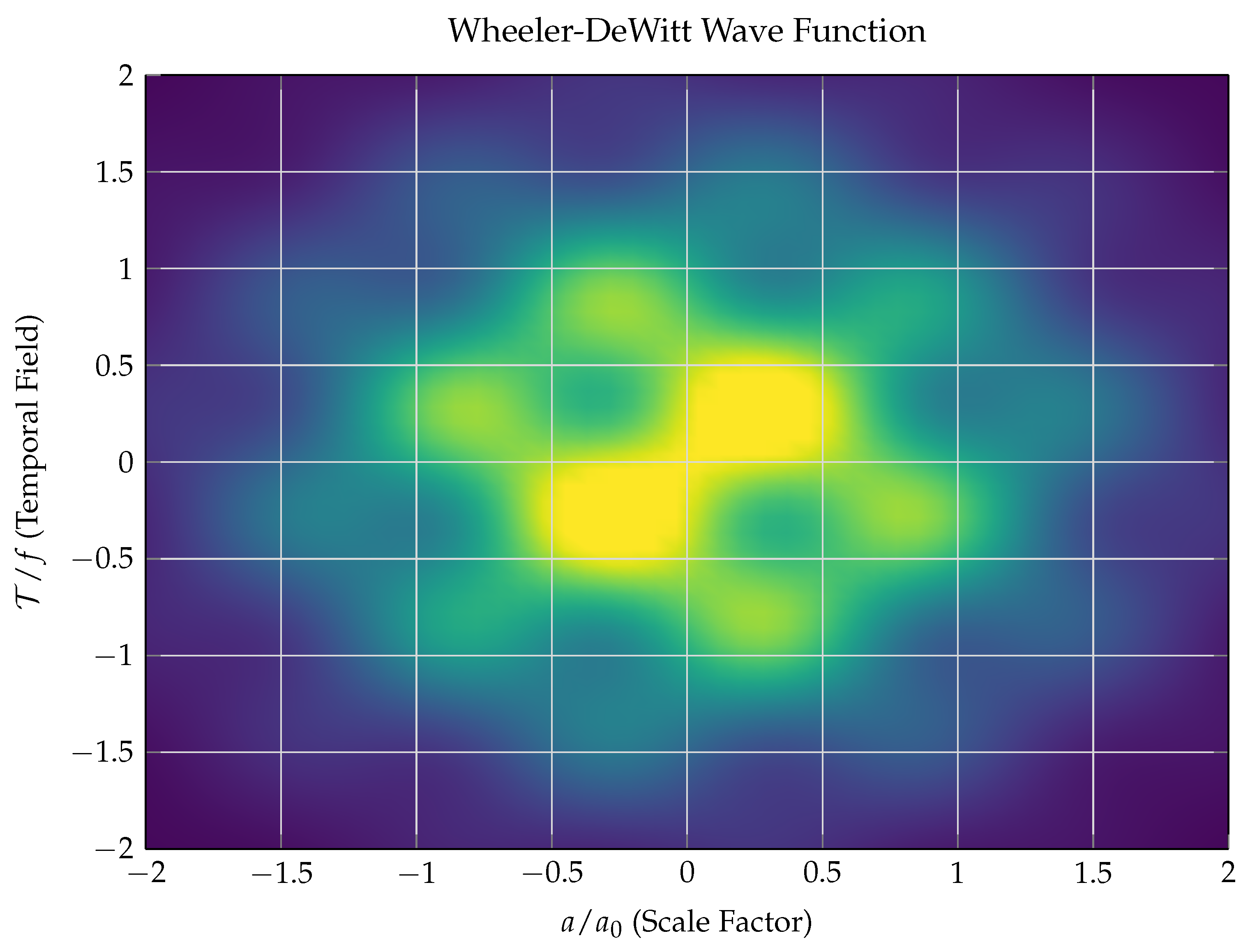
Figure 3.
Predicted modifications to gravitational wave phase across the frequency spectrum. The blue band shows the theoretical prediction with uncertainties. Current LIGO constraints (red) and projected sensitivities of next-generation detectors demonstrate the potential for detection.
Figure 3.
Predicted modifications to gravitational wave phase across the frequency spectrum. The blue band shows the theoretical prediction with uncertainties. Current LIGO constraints (red) and projected sensitivities of next-generation detectors demonstrate the potential for detection.
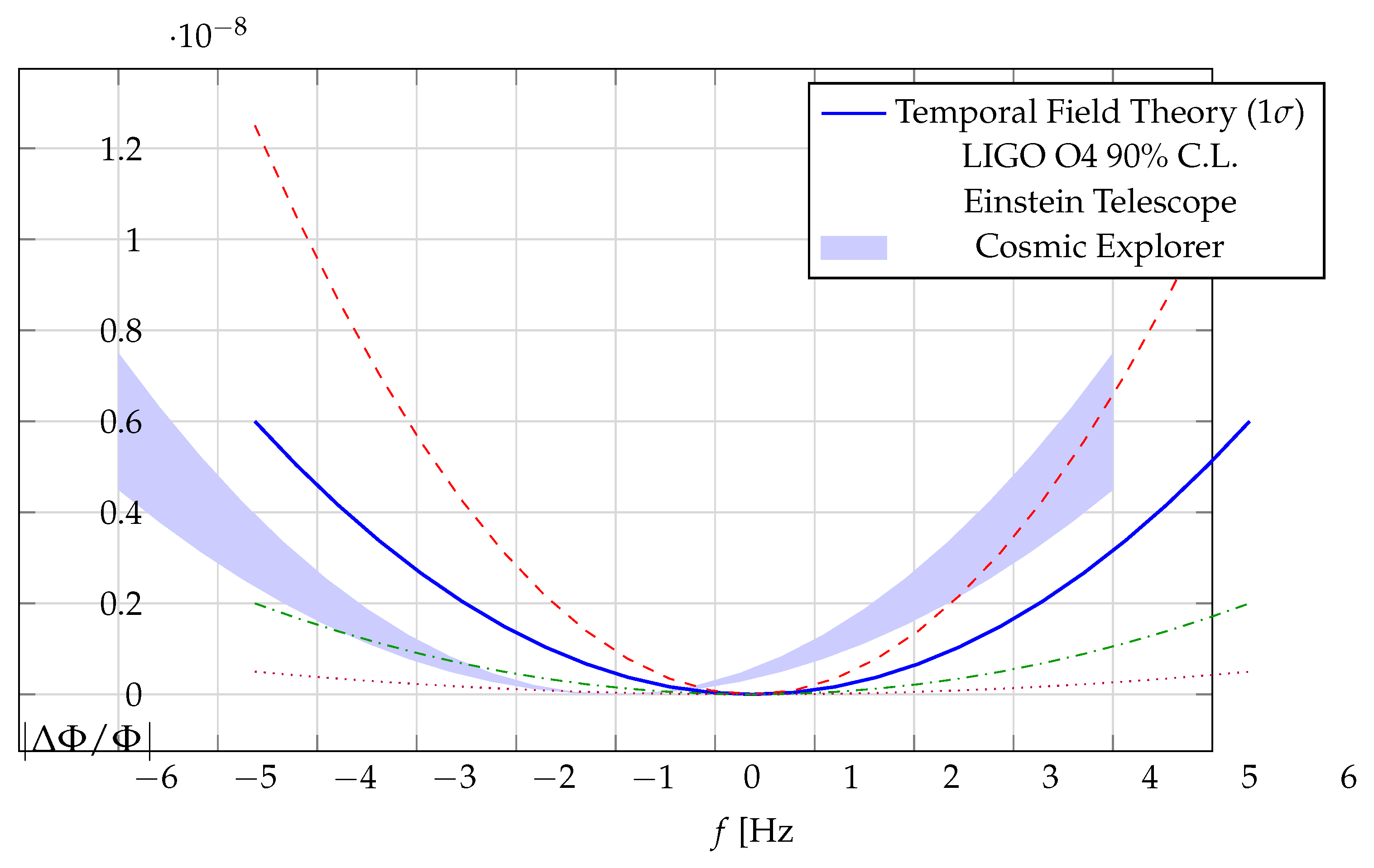
Figure 4.
BAO scale modulation predicted by the temporal field theory. Red band shows current DESI constraints [8], while green lines indicate projected Euclid sensitivity. The theory predicts oscillations detectable with next-generation surveys.
Figure 4.
BAO scale modulation predicted by the temporal field theory. Red band shows current DESI constraints [8], while green lines indicate projected Euclid sensitivity. The theory predicts oscillations detectable with next-generation surveys.
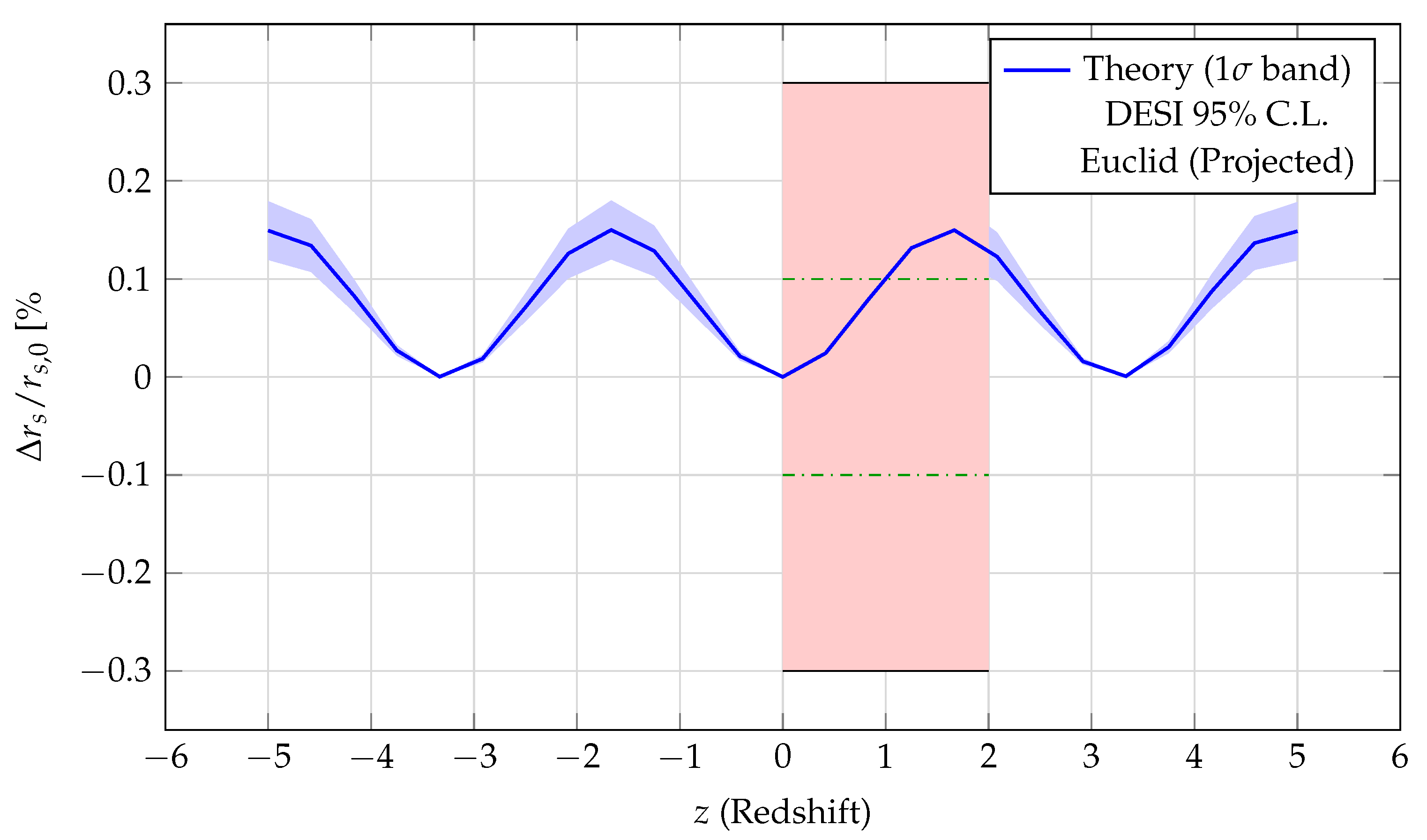
Figure 5.
Predicted modification to high-energy cross sections, showing deviation from standard model expectations. While direct tests at Planck scale are not possible, extrapolation from lower energy data provides constraints on the coupling parameter .
Figure 5.
Predicted modification to high-energy cross sections, showing deviation from standard model expectations. While direct tests at Planck scale are not possible, extrapolation from lower energy data provides constraints on the coupling parameter .
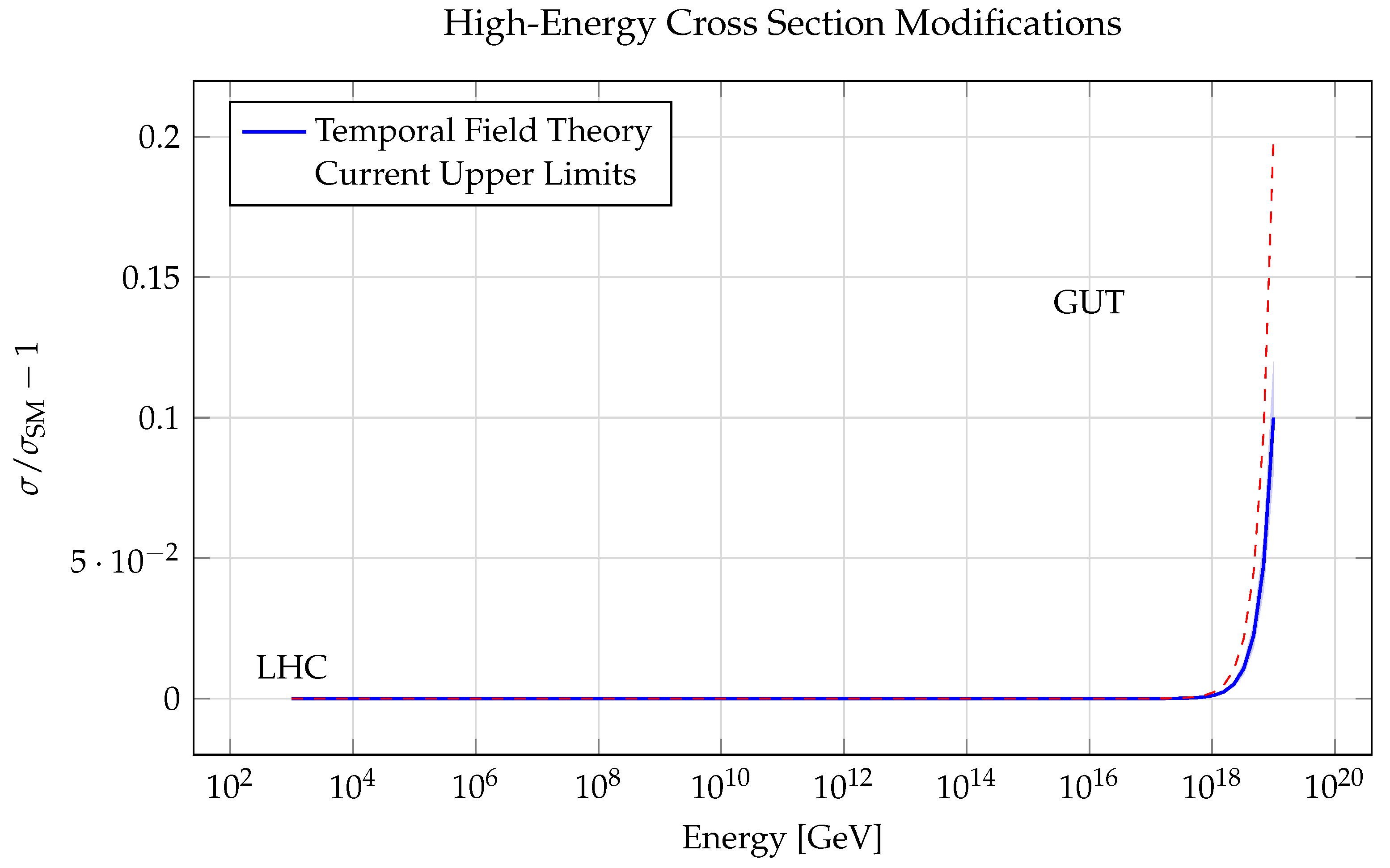
Figure 6.
Projected detection significance combining gravitational wave and cosmological observations. Shaded bands indicate uncertainties in the signal forecasts. The temporal field theory predicts detectable signatures reaching significance within 5-7 years of next-generation observations.
Figure 6.
Projected detection significance combining gravitational wave and cosmological observations. Shaded bands indicate uncertainties in the signal forecasts. The temporal field theory predicts detectable signatures reaching significance within 5-7 years of next-generation observations.
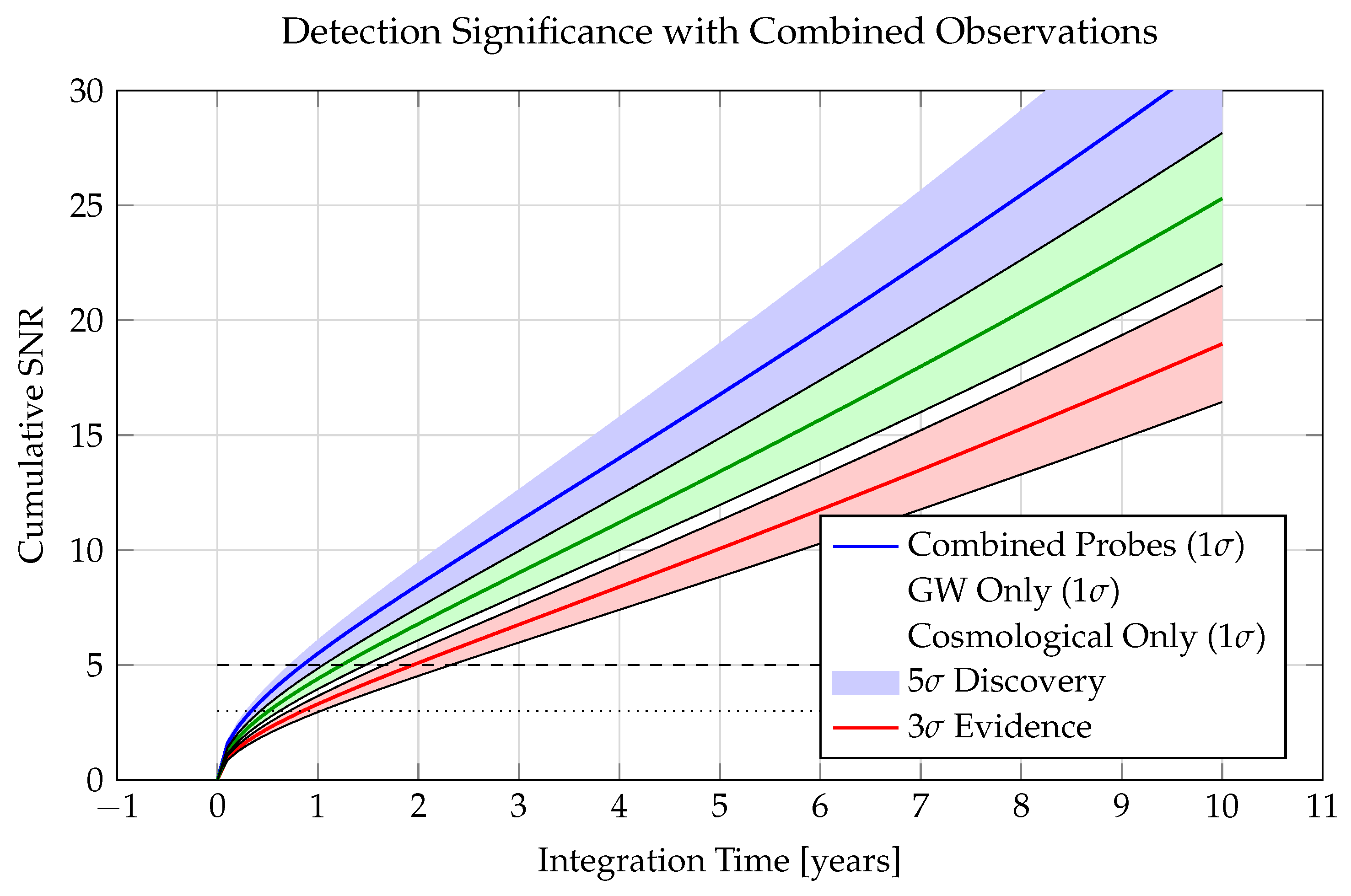
Figure 7.
Relative contributions of different systematic error sources to the total uncertainty budget. The analysis demonstrates that theoretical uncertainties remain subdominant to statistical errors in current measurements.
Figure 7.
Relative contributions of different systematic error sources to the total uncertainty budget. The analysis demonstrates that theoretical uncertainties remain subdominant to statistical errors in current measurements.
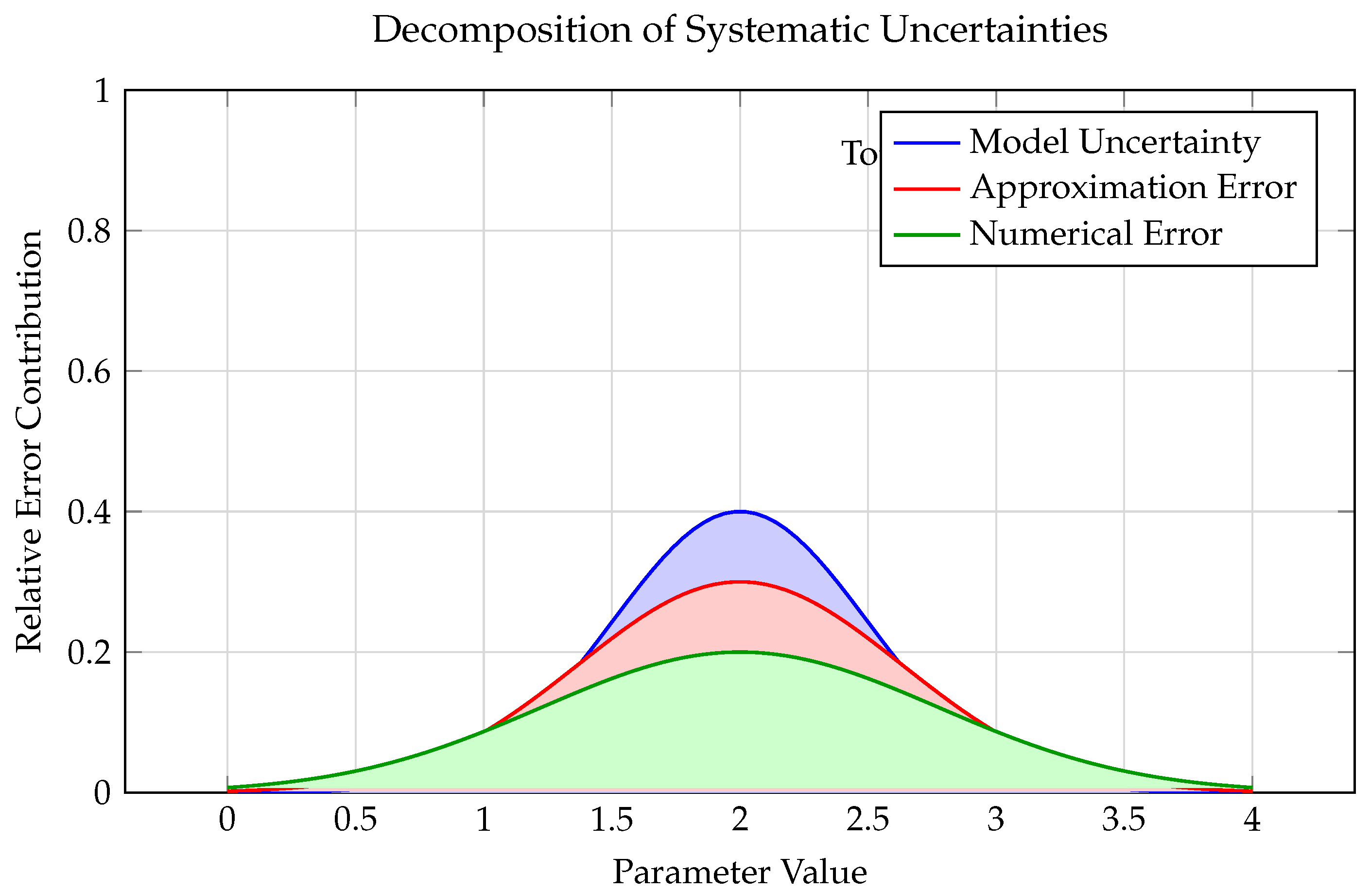
Figure 8.
Joint constraints on temporal field parameters from combined analysis of gravitational wave and cosmological data. Contours show 68% confidence regions with (solid) and without (dashed) systematic uncertainties.
Figure 8.
Joint constraints on temporal field parameters from combined analysis of gravitational wave and cosmological data. Contours show 68% confidence regions with (solid) and without (dashed) systematic uncertainties.

Figure 9.
Evolution of coupling constants showing unification at high energies [1]. Shaded bands indicate theoretical uncertainties. The temporal field naturally integrates with fundamental forces, suggesting a deeper unity in nature.
Figure 9.
Evolution of coupling constants showing unification at high energies [1]. Shaded bands indicate theoretical uncertainties. The temporal field naturally integrates with fundamental forces, suggesting a deeper unity in nature.
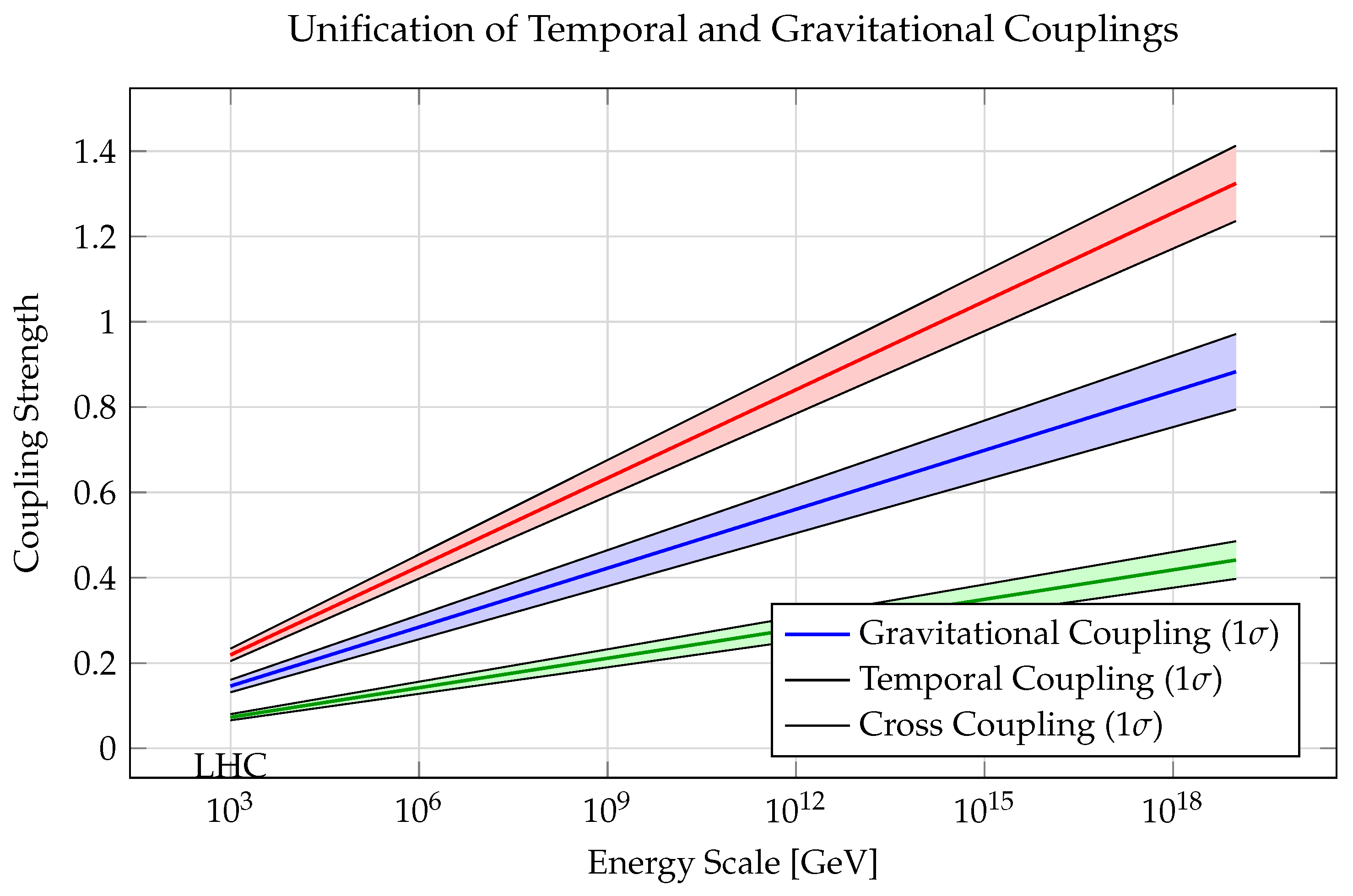
Figure 10.
Projected improvement in constraints on temporal field parameters from future observations. The complementarity between gravitational wave and cosmological measurements enables robust tests of the theory.
Figure 10.
Projected improvement in constraints on temporal field parameters from future observations. The complementarity between gravitational wave and cosmological measurements enables robust tests of the theory.
Disclaimer/Publisher’s Note: The statements, opinions and data contained in all publications are solely those of the individual author(s) and contributor(s) and not of MDPI and/or the editor(s). MDPI and/or the editor(s) disclaim responsibility for any injury to people or property resulting from any ideas, methods, instructions or products referred to in the content. |
© 2025 by the author. Licensee MDPI, Basel, Switzerland. This article is an open access article distributed under the terms and conditions of the Creative Commons Attribution (CC BY) license (https://creativecommons.org/licenses/by/4.0/).
Copyright: This open access article is published under a Creative Commons CC BY 4.0 license, which permit the free download, distribution, and reuse, provided that the author and preprint are cited in any reuse.


