

Submitted:
07 June 2024
Posted:
10 June 2024
You are already at the latest version
Abstract
Rural electrification is a crucial step for the socio-economic development of isolated communities. Decentralized power generation, typically more favorable for renewable energies, requires an accurate analysis of the different electrification options, whose convenience depends on multiple factors. The application of Geographical Information System (GIS) to energy planning allows the assessment at a local level, considering spatial resources variability and demand distribution. This work introduces IntiGIS-local, a GIS-based model implemented in ArcGIS environment, designed to calculate the Levelized Energy Cost (LEC) for different electrification options. The model allows the comparison between three power generation alternatives: solar system, diesel generator set and solar-diesel hybrid system. Configurations are adjustable through input variables, with a special focus on the confrontation between individual systems and microgrids. The objective is to provide an adequate groundwork for developing a decision-making tool to assess diverse rural electrification options in future studies. The model IntiGIS-local is tested in the case study of Guasasa community (Cuba).
Keywords:
Renewable Energy
; Hybrid Systems
; PV
; Rural Electrification
; Microgrid
; GIS
; Spatial Analysis
; Mapping
; Geo-modelization
1. Introduction
Access to electricity is an essential requirement for human development. It is recognized as a basic need to ensure the respect of human rights and the improvement of life quality. In 2019, one year before the COVID-19 pandemic was declared, more than 800 million people in the world were still without access to electricity, of whom almost 600 million are in Sub-Saharan Africa [1]. The effects of COVID-19 could be dramatic, as noted by the International Energy Agency (IEA) in its latest report [2], where is remarked that “The (…) pandemic has caused more disruption to the energy sector than any other event in recent history, leaving impacts that will be felt for years to come”. In this sense, vulnerable population (most in rural areas) will feel the “worst effects”. As examples, the report points out that “the number of people without access to electricity in sub-Saharan Africa is set to rise in 2020” and more than 100 million people, with electricity access in 2019, will lose the conditions achieved and return to energy poverty parameters. This situation continues to this day and remains a pressing and topical issue.
Along with IEA’s, several studies include this point of view in new scenarios, reinforcing the idea from multiple perspectives, especially from the perspective of the impact on demand and the growth of energy poverty [3,4,5,6,7,8,9,10,11,12,13,14,15,16,17,18,19,20,21,22,23,24,25].
Despite the pandemic, during the recent years, the worldwide energy policies are strongly committed in reducing these numbers. The trend was positive: in 2017, the population without electricity amounted to almost 1 billion, so the improvement is promising. The progress is concentrated in some areas, especially in Asia, which accounts for 80% of the 800 million people who gained access since 2000. Nearly two-thirds of them are attributable to India. The target of reaching 100% of the electrification rate has a major issue: especially in developing countries, the welfare provided by the new energy availability is likely to induce a positive feedback by further increasing the population growth rate, thus increasing the population target. As a consequence, the effort to pursue this challenge must be held constant [1].
One of the United Nation’s Sustainable Development Goals is to reach universal access to clean and affordable energy by the year 2030 [26]. In the Sustainable Development Scenario (SDS), considering an expected strong population growth, this goal would require a cumulative total of more than 1 billion people to be supplied by new energy access. In economic terms, it has been estimated that the process would require an average investment of $40 billion per year [1]. According to the Stated Policies Scenario (SPS), so assuming to keep the current and announced policies, the improvements would be considerably slower. In particular, in Sub-Saharan Africa the actual rate of annual connections would require a triplication.
Renewable energies represent the key to achieve this ambitious target while preserving sustainability and contribute to improve a best post-pandemic scenario. In many areas they would also be the least expensive option contributing to mitigate the energy poverty. The advantages of renewable energy in its various forms is the unrestricted availability all around the world and their declining costs, even in areas where the distribution of conventional energy sources is inconvenient. A peculiarity is its typical variability, both in time and space, which can undermine a reliable power supply. A careful assessment of the available energy mix is therefore a fundamental step in the early stage of an electrification plan. Several factors are involved in this process and they are often detectable at a local level.
In this sense, the present work aims to provide a decision-making tool for rural electrification developments, using Geographical Information Systems (GIS). It is focused on the implementation of hybrid systems, optimizing renewable contribution and local resources [27,28,29,30].
1.1. Rural Electrification & GIS
There are two general approaches to the electrification of isolated areas: through the extension of the national grid or by the implementation of off-grid systems. The first one is by far the most common, including the 99% of electricity infrastructure investments from utilities and governments [31]. The off-grid option prevails when some specific conditions penalize the extension, usually due to an excessive distance from the existing grid. In this sense, it is important to be able to estimate the cost associated to both cases, in order to choose the most convenient option for each circumstance. The cost clearly rises with the increase of the distance to be covered by the grid extension, while the cost of the off-grid option can be considered independent from the distance [32].
It is evident that isolated communities are the most affected by lack of electrification access, due to several aspects that discourage the investors [33]. The main critical aspects of rural electrification are typically the low density load and the high installation, operation and maintenance costs which lead to a long investment return period [34].
Two main categories of off-grid electrification options can be identified: centralized systems and individual systems. A centralized system requires the construction of a microgrid (also referred as mini-grid) that connects all the loads to the central power plant. In cases of sufficient diversified available energy mix, a hybrid plant, which combines different types of technologies, can be an effective option. Individual systems are designed to supply energy to each building autonomously. Typical examples are: photovoltaic (PV) stand-alone systems, small wind turbines or small diesel generators. The choice of the best option and the most convenient configuration can be challenging. The objective of this work is to facilitate this task [35].
Given this consideration, the assessment of Renewable Energy Sources (RES) becomes crucial for aligning power supply and energy demand. Spatial and temporal variability play a crucial role in this process.
GIS represents an instrument capable to integrate non-spatial features (technological, economical, etc.) in a local reality, not only intended from a geographical point of view, but also from the perspective of a network of mutually related activities [36].
Therefore, the wide geographical dispersion that characterizes RES and the importance of evaluating their integration at a local level fit perfectly with the potential of GIS analysis. The scientific literature that reinforces this aspect is numerous. There are a large number of studies linking the application of GIS with renewable energies in general and with their development in rural areas in particular [37,38,39,40]. Many studies have been developed in Africa [41,42,43,44,45,46,47,48,49,50] or Asia [51,52,53,54,55,56] and, to a lesser extent, in Latin America [57,58,59]. Some are focused on stand-alone installations [45,60,61,62] and others on grid connections [63]. In some cases, the development of specific GIS as OnSSET [42,64] or IntiGIS [65,66] for rural electrification planning is the first goal. In this way the Reference Electrification Model (REM) allows identifying the lowest cost designs that provide access to electricity in large-scale areas [67]. However, this task force has also developed a particular REM configuration, called LREM (Local REM), which provides detailed electrification designs where all consumers are connected to a single mini-grid applied in India, Nigeria, and Rwanda.
1.2. Purpose of the Work
The primary objective of this research is to develop a GIS-based model for the techno-economic assessment of rural electrification plans, taking into account the spatial distribution of demand and resources. The considered technologies are: PV system, diesel generator set and their combination in a hybrid system with storage. The resulting comparison of different power system configurations will inform the decision-making process for evaluating the best electrification option. The study is focused on spatial analysis to assess several combinations of PV home systems and PV based microgrids. This last aspect is innovative, even in the design of microgrids for urban PV systems not connected to the general grid. The potential of this approach is very interesting to develop new rural electrification studies, emphasizing the combined optimization of different domestic PV systems and the hybridization of various configurations with other renewable and conventional sources.
The study employs ArcGIS software. This paper focuses on implementing and testing a specific model developed within ModelBuilder, used to create, edit and automate geoprocessing models. The model involves a series of calculations between the attributes of various loads, each properly conFigured for specific simulation. The equations are derived from the original IntiGIS model, extensively reviewed and adapted to the structure of the new one, named IntiGIS-local. The main result of the set of equations is the Levelized Energy Cost (LEC) of the power plant considered for the simulation, also referred as Levelized Electricity Cost or Levelized Cost of Energy (LCOE). The LEC allows the comparison of different electricity generation methods, by summing all costs incurred over the power plant lifetime and the total amount of energy produced. Essentially, it quantifies the average total cost of producing one unit of energy.
After discussing the model structure, it is applied to the case study of the community of Guasasa (Cuba). The input assumptions are set, drawing information from the existing studies. The model is designed to be adaptable for any case, serving as the groundwork for a more complete tool in future developments. From this perspective, the simulation results are analyzed, comparing different proposed configurations.
In summary, this paper is structured in two main parts: the implementation of a model for the LEC calculation of different types of power plant using GIS; and the test of the model for the case study of Guasasa.
The study's conclusions allow for an optimistic approach to a planned electrification strategy based on hybrid microgrids. In this sense, the Cuban authorities are firmly committed to this technology, which combines access to energy, the use of local resources, the promotion of social dynamics in small isolated communities, fuel savings and energy independence.
2. LEC Modelling in a GIS Environment
The present section introduces the model IntiGIS-local, developed through ModelBuilder for calculating the LEC of different possible power plants types. The input required is a point feature class [68] representing the group of buildings to be supplied, whose attribute Table [68] contains data of energy demand of each building, along with certain cost and lifetime assumptions. By adapting the input to the specific case under consideration, the model can be applied to any selected group of buildings.
The types of power plants included in our methodological proposal are the following:
- Photovoltaic Stand-alone System (for each individual building);
- Photovoltaic Centralized System;
- Solar-Diesel Hybrid System (centralized system);
- Diesel Generator Set (centralized system).
The selection of these technologies has an eminently operational character, as they are the most widespread configurations in most off-grid electrification proposals. In future developments, further typologies will be integrated, considering other energy resources, to provide a complete picture of the rural electrification options.
2.1. Methodology
The origin of this methodology comes from the project SOLARGIS, financed by the Directorate General XII for Science, Research and Development of the European Commission that involved many research centers in the nineties [69]. This development confirmed the importance of a local perspective in renewable energies integration processes and the great potential of GIS technologies in this contribution. A first update was released in the second phase, SOLARGIS II, as part of the agreement between CIEMAT (Center for Energy, Environmental and Technological Research) and the UPM (Polytechnic University of Madrid) with the aim of defining the degree of uncertainty of the model execution [70]. With this basis, IntiGIS model was created: a plug-in of ArcGIS, developed without commercial purpose, to support the electrification planning of rural, isolated areas [65,71]. At the actual stage, IntiGIS has been tested in different study sites and is still subject to improvements. The model allows to compare several technology options: photovoltaic, wind power, diesel generator, hybrid photovoltaic-diesel, hybrid wind-diesel and grid extension. Further upgrades are under investigation, such as the addition of the biomass option. However, the main issue is now to improve the Information Technologies (IT) aspect, fixing some bugs that can undermine the smoothness of the operation.
The study focuses in solar energy in comparison with diesel power generation and their combination in a hybrid system. The main update introduced is designed to facilitate the comparison between individual and centralized systems. In the original model [70], the energy demand is expressed in the form of a raster representing the building density. The LEC calculation is performed pixel by pixel, allowing to visualize the most competitive technology to supply the energy demand of each cell. This approach provides an immediate visual impact in the comparison between different technologies. On the other hand, its weakness is not allowing a combination of different groups of buildings in a microgrid.
The new model, IntiGIS-local, proposes a solution to this issue. While introducing the input map that contains the energy demand distribution, the user can select a group of buildings to be supplied through a centralized power system. The unselected buildings will be assigned by default to the individual system case. In this way, it is possible to simulate the techno-economic performance of different configurations of microgrids and, at the same time, compare them with the individual option. Another key point introduced for the centralized case consists on the visualization of the resulting LEC in raster format. The choice of the installation site can have a high impact on the cost of generation, due to spatial variability of the resources combined with the distance from the main distribution line. In some cases, the most cost-effective solution does not correspond to the closest location to the central line. The resulting raster defines where it is more convenient to place the centralized plant. Each pixel represents the LEC value of a hypothetical plant placed in the same pixel, capable to fulfill the demand of the selected microgrid.
The boundaries of the system defined for the centralized cases include the cost associated to the potential grid construction or extension. Being primarily designed for small communities, a low voltage grid is considered, so transmission lines and transformers are not included. Tax, subsides, environmental and public health impact are not taken into account in the cost assessment but could be studied for future developments.
2.1.1. General Parameters
The equations of the model are basically defined upon the following parameters:
- (years): Expected Lifetime of the subsystem “i”;
- : Discount Rate;
- : Capital Recovery Factor for the subsystem “i”
- (€/kW): Capital Investment for the diesel generator per unit of power;
- (€/kWp): Capital Investment for the solar panels per unit of peak power;
- (€/kWh): Capital Investment for the storage per unit of capacity;
- (€/kW): Capital Investment for the power conditioning per unit of power;
- (€/km): Capital Investment for the distribution line per unit of length;
- (€/kW): Capital Investment for the grid connection per unit of power;
- (€/(hop·kW)): Operation & Maintenance (O&M) cost for the diesel generator per units of operating hours per kW;
- (€/kWp): O&M annual cost for the solar panels per unit of peak power;
- (€/kWh): O&M annual cost for the storage per unit of capacity;
- (€/kW): O&M annual cost for the power conditioning per unit power;
- (€/km): O&M annual cost for the distribution line per unit of length;
- (h): Hours per year;
- (kWh): Daily Energy Demand for a single building;
- (kW): Contracted Power for a single building;
- : Capacity Factor for the power generation technology “i“;
- (€cents/kWh): Cost of the subsystem “i“ per unit of energy produced;
- (€cents/kWh): Levelized Energy Cost of the power plant “i“.
The Capital Recovery Factor is the ratio used to calculate the present value of an annuity (a series of equal annual cash flows).
The Capacity Factor is the ratio of the actual energy output over a period and the maximum possible energy output over the same period. The period considered is one year.
2.1.2. Individual Power Plants: PV Stand-Alone
The Levelized Energy Cost of a photovoltaic stand-alone power plant is calculated as the sum of the cost per kWh of three subsystems: PV modules, Storage and Power Conditioning.
PV Levelized Energy Cost (€cents/kWh):
The PV Modules cost (€cents/kWh) is calculated as follows:
is the Capacity Factor of the photovoltaic system:
where:
- is the global efficiency of the photovoltaic system;
- is the the maximum efficiency of the solar panel at standard conditions (Irradiance: ; Temperature: ; AM 1.5);
- is the total Area covered by the solar panels;
- (kWh/m2) is the average annual Global Irradiation on tilted surface (with inclination angle of the solar panel);
- is the Peak Power (kW) of the solar system, equal to:
Since the irradiance at standard conditions is equal to 1 kW/m2, equation 4 can be simplified as follows:
The value of the annual global irradiation can be therefore expressed both in units of energy per squared meters (kWh/m2) and in equivalent hours at 1 kW of irradiance (heq,stc). Once obtained the capacity factor of the photovoltaic system, the required installed power capacity (kW) can be calculated from:
where:
- is the annual energy demand for a single building () (kWh).
The Storage cost (€cents/kWh) is calculated as follows:
is the Storage Capacity (kWh):
where:
- [days] is the autonomy of the storage. It represents the maximum period in which the battery can satisfy the energy demand by itself;
- is the Depth of Discharge of the battery;
- is the efficiency of the storage.
The Power Conditioning cost (€cents/kWh) is calculated as follows:
The Power Conditioning refers to the Balance of System excluding the storage. It is mainly composed by the inverter.
is the Inverter Load Factor for a stand-alone PV system, which can be seen as the ratio between the average operating power and the maximum admissible power of the inverter. It is convenient to express this relation as a function of the energy load characteristics, which are described by the shape of the demand curve. The Load Factor () is the ratio between the Average Load () and the Peak Load () of the energy demand:
In the calculation of the inverter load factor, the conversion efficiency needs to be considered. The efficiency depends on the percentage of the load supply, on the type of inverter chosen and on the value of the input voltage [72]. A correction factor () is therefore introduced which can include other adjustments experimentally derived in order to associate the proper weight to the cost of the power conditioning. For example, the inverter is normally designed with a higher maximum admissible power than the peak load, so an oversized coefficient affects the inverter load factor.
where:
- is the nominal efficiency of the inverter for a PV stand-alone system.
2.1.3. Centralized power plants: Diesel, PV centralized, Hybrid Solar-Diesel
The LEC model considers three possible configurations for the centralized case:
- Diesel generator set;
- Photovoltaic centralized;
- Solar-Diesel Hybrid system.
All the centralized configurations are defined by the same algorithm. The discriminating factors between one case and the others are the input settings of the model. In particular, a crucial parameter is the Renewable Fraction, representing the percentage of power generation from renewable sources in the total energy production:
- Diesel generator set;
- Photovoltaic centralized;
- Solar-Diesel Hybrid system.
The ArcGIS model allows to select a group of buildings to be supplied with a centralized power plant. The aggregated annual energy demand (kWh) is the sum of the annual energy demands of each building “i” selected (kWh):
Once established the renewable fraction, the annual energy produced by the photovoltaic system (kWh) can be calculated:
The annual energy produced by the Diesel generator system (kWh) is the residual energy demand to be fulfilled:
The Levelized Energy Cost of a centralized power plant is calculated as the sum of the cost per kWh of seven subsystems: PV modules; Storage system; Power Conditioning system; Diesel generator; Fuel; Line; Connections.
The centralized PV Modules cost (€cents/kWh) is calculated as follows:
is the Capacity Factor of the centralized photovoltaic system:
where:
- is the global efficiency of the centralized photovoltaic system.
Once the capacity factor of the centralized photovoltaic system has been obtained, the required installed power (kW) can be calculated based on:
The centralized Storage cost (€cents/kWh) is calculated as follows:
is the centralized Storage Capacity (kWh):
where:
- (days) is the autonomy of the centralized storage. It represents the duration in which the battery can satisfy the aggregated energy demand by itself;
- is the Depth of Discharge of the battery used in the centralized storage;
- is the efficiency of the centralized storage.
The centralized Power Conditioning cost (€cents/kWh) is calculated as follows:
is the power conditioning Load Factor for a centralized system, to which the same considerations apply as for individual systems:
where:
- is the conversion efficiency of the centralized power conditioning. It includes in a single parameter the effect of the whole set of power electronics (inverters, rectifiers and/or bidirectional inverters)
A standard centralized system generates the power in AC and feeds the load directly. In parallel, an AC to DC conversion is necessary to charge the battery. Finally, the central inverter converts again the output power of the storage. The contribution of the power conditioning to the LEC of a centralized plant is higher than an individual one. The investment for the rectifier system is taken as 50% of the cost associated to the central inverter [72]. A correction factor of 1.5 is therefore applied to take into account the higher complexity of the centralized system in comparison to the individual case.
The Diesel generator set cost (€cents/kW) is composed of the generator cost (€cents/kW) and the reconstruction cost (€cents/kW):
The distinction between these two factors was introduced to provide a more accurate reflection of the costs associated with replacing damaged components. Initially, the period before the first replacement was excessively penalizing compared to real-world scenarios, especially in the context of diesel generators. By separating out the reconstruction cost, we are able to assign a higher value to the expected lifetime of the diesel generator, resulting in a more realistic distribution of capital investment costs over its lifetime.
The Diesel Generator cost (€cents/kWh) is calculated as follows:
The Reconstruction Cost (€cents/kWh) is calculated as follows:
is the Capacity Factor of the Diesel generation set:
is the required installed Power capacity (kW) of the diesel generator set:
where:
- is the contracted power (kW) of each building to be supplied by the centralized power plant;
- is the Design Factor of the diesel generator, to be set according to the simultaneity of the individual loads and an oversize factor.
The size of the diesel set needs to guarantee the supply of the aggregated load peak power with a safety margin. should always exceed the load plus 2.5 or 3 times the power of the battery charger [70]. For this reason, the design factor needs to have a higher value than the coincidence factor of the individual loads.
In the hybrid case, the diesel generator size does not depend on the renewable fraction of the system. It plays a backup role in the system, so it should be able to autonomously feed all the centralized loads in case of need.
The Fuel Cost (€cents/KWh) is calculated as follows:
where:
- is the Fuel Consumption (l/kWh) of the diesel generation set;
- is the Fuel Price (€/l).
The Line Cost (€/kWh) is calculated as follows:
is the Total Line Length (m), automatically calculated by the ArcGIS model and equal to:
where:
- is the length of the central line;
- is the distance between the installation site of the centralized power plant and the central line, following the shortest path;
- is the distance between the load “i” and the central line, following the shortest path.
Note that the requested line costs inputs are expressed in units of €/km.
The Connection Cost (€cents/kWh) is calculated as follows:
Such factor is associated with the expenditure for each load connection to the grid.
2.2. Model Structure
IntiGIS-local requires the following input data:
- Map of the buildings to be powered: a point feature class file representing the position of each building considered for the electrification plan;
- Map of the buildings to be powered by a microgrid: a point feature class file representing the position of the group of building considered for the centralized system;
- Hypothetical central line: a polyline feature class file representing the central distribution line of the microgrid to which all the buildings would be connected in case of full centralization;
- Average annual global solar radiation raster on a tilted surface (solar panel optimal angle);
- Digital Elevation Model (DEM) of the study area.
The input parameters can be set through the attribute tables of the first two maps. Every building can be characterized by entering the daily energy demand and the peak power, while all the economic and technical factors can be introduced on the related columns of the attribute table. Depending on the power system configuration chosen and the socio-economic background, the user defines: investment and O&M cost of each subsystem, efficiency and lifetime of the components, days of autonomy and depth of discharge of the battery, renewable fraction, fuel cost and all the other variables required by the equations introduced in paragraph 2.1.
The algorithm is structured in two macro-areas, one referred to the stand-alone solution and the other to a microgrid, leading to a simultaneous calculation of the LEC for both the individual and the centralized systems. In the first case, the only available configuration is the photovoltaic system, while the microgrid could be a photovoltaic, diesel or hybrid solar-diesel system, basing on the input settings.
Through the combination of some ArcGIS tools, a polygon is created to represent the reference area of the centralized system. This polygon is generated with a buffer surrounding the selected buildings for the microgrid, applying an arbitrary value of distance. Subsequently, this layer is used to extract the group of buildings that will be powered by individual systems from the map representing the whole group of buildings. Moreover, it aids in deriving the required portion of the central line for the microgrid, by removing all the unnecessary sections from the hypothetical central line.
Once obtained the central line of the microgrid, two more components are needed to calculate the total line length: the distance between the installation site of the centralized power system and the central line, and the distance between every building and the central line (refer to equation 31). Both factors are calculated for the shortest path, considering potential obstacles and altitude variations, based on the information from the DEM of the study area. The result is a raster depicting the total distribution line length, with each value representing the line length considering the installation site located in the center of the cell.
At this stage, the LEC calculations can be performed. For the stand-alone system, each building is associated to the annual solar radiation it receives, extracted from the solar radiation raster. The subsystem costs are calculated and summed to derive the LEC for each individual power system. The results are displayed over each building of the map excluded from the microgrid. For the centralized system, calculations are performed for each cell of the raster, referring to the corresponding values of solar radiation and line length for possible installation sites. By summing all subsystem costs in raster format, the result is the LEC of the centralized power system for the chosen configuration. The fluctuation of its value, depending on the installation site, can be visualized through a color gradient. The structure of the model IntiGIS-local and its main steps are summarized in the Figure 1. An alternative version of this chart in ModelBuilder format for ArcGIS is available in [73].
3. Results for LEC Calculation: the Case of Guasasa
3.1. Context of the Case Study
IntGIS-local is tested in the context of HIBRI2: “Integrated control system for energy supply through hybrid systems in isolated communities in Cuba. Phase II” [74]. The action is included in the innovation schemes funded by the AECID (Spanish Agency for International Development Cooperation) and coordinated by CIEMAT, under the Spanish Ministry of Science and Innovation. The partners are, in the Spanish side: SODEPAZ Non-Governmental Organization (NGO) and Bornay company, and in the Cuban side: Cubasolar NGO and CUBAENERGÍA research center. The target of the cooperation action is to complete the electrification of the small isolated community of Guasasa (Cuba) [75]. It constitutes a continuation of the mission HYBRIDUS, with the objective of promoting the integration of renewable energies in different Cuban locations. HYBRIDUS operates actively many projects, among which it is worth mentioning the realization of a cogeneration system to help agricultural exploitations in the municipality of Guamá, located in Santiago de Cuba province [76].
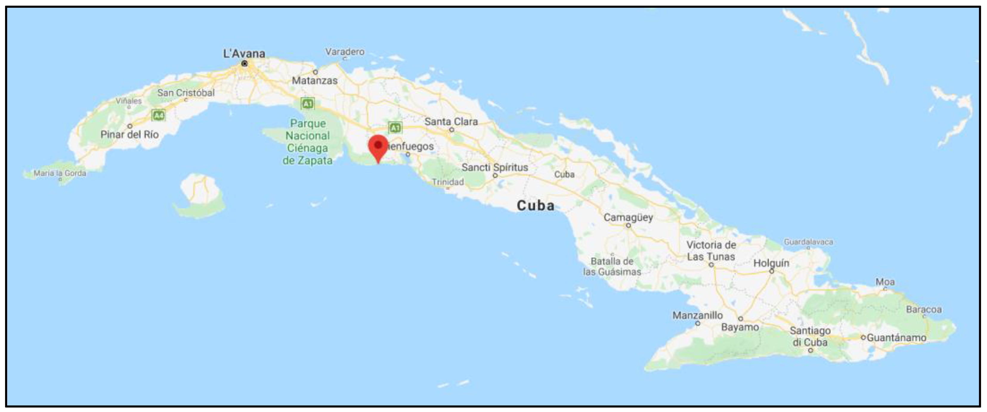
IntiGIS-local has been tested for the case of Guasasa, a small isolated community in the southern coast of Matanzas province (Cuba). It is part of the southern coast overlooking the Caribbean Sea and its geographic coordinates are: 22° 38’ 0” North; 83° 43’ 0” East.
Figure 2.
Location of Guasasa, Cuba (source: Google Maps).
The climate is characterized by warm temperatures during the whole year, with an average annual temperature of 24.5 ℃.

Table 1.
Average temperatures (ºC) in Guasasa, registered during a period of 25 years (1983-2005) (Source: NOAA [77]).
Table 1.
Average temperatures (ºC) in Guasasa, registered during a period of 25 years (1983-2005) (Source: NOAA [77]).
| Month | Jan | Feb | Mar | Apr | May | Jun | Jul | Aug | Sep | Oct | Nov | Dec | Annual |
| Average temperature | 21 | 22 | 24 | 25.3 | 26 | 26 | 26 | 26.4 | 26 | 25 | 24 | 22 | 24.5 |
The population of Guasasa is composed of 214 people and the principal activity of the community is fishing, which constitutes almost the 60% of the economy. The remaining percentage is characterized by forestry service (25%) and other community works [78].
3.2. Existing Grid
The actual level of electrification is provided by a diesel generator set which feeds the village for a total of 12 hours a day. The target is to provide a continuative energy supply (24 hours a day) through the integration of several renewable energies (biomass, PV and wind), in order to support the social and economic development of the community. In addition to the direct benefits for Guasasa, the action will constitute an important educational and information source for further applications in other zones of the island. A description of the existing diesel generator set and the low voltage feeder is presented, as they will be used for the Base Case “Real” scenario.
Figure 3.
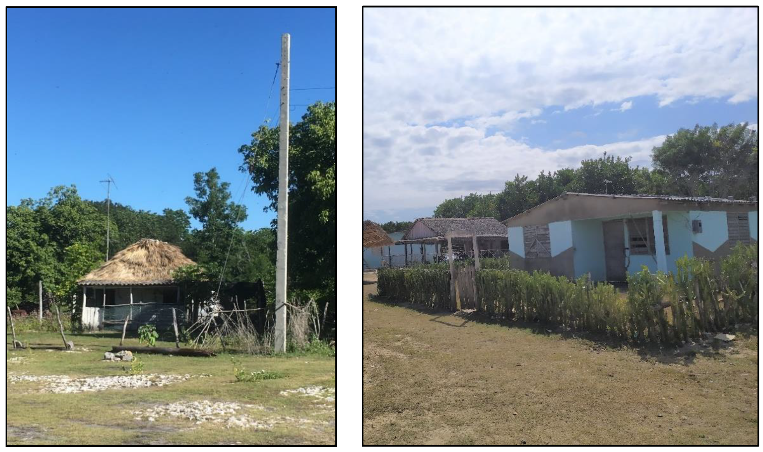
Some examples of typical houses in Guasasa community (source: authors).
3.2.1. Diesel Generator Set
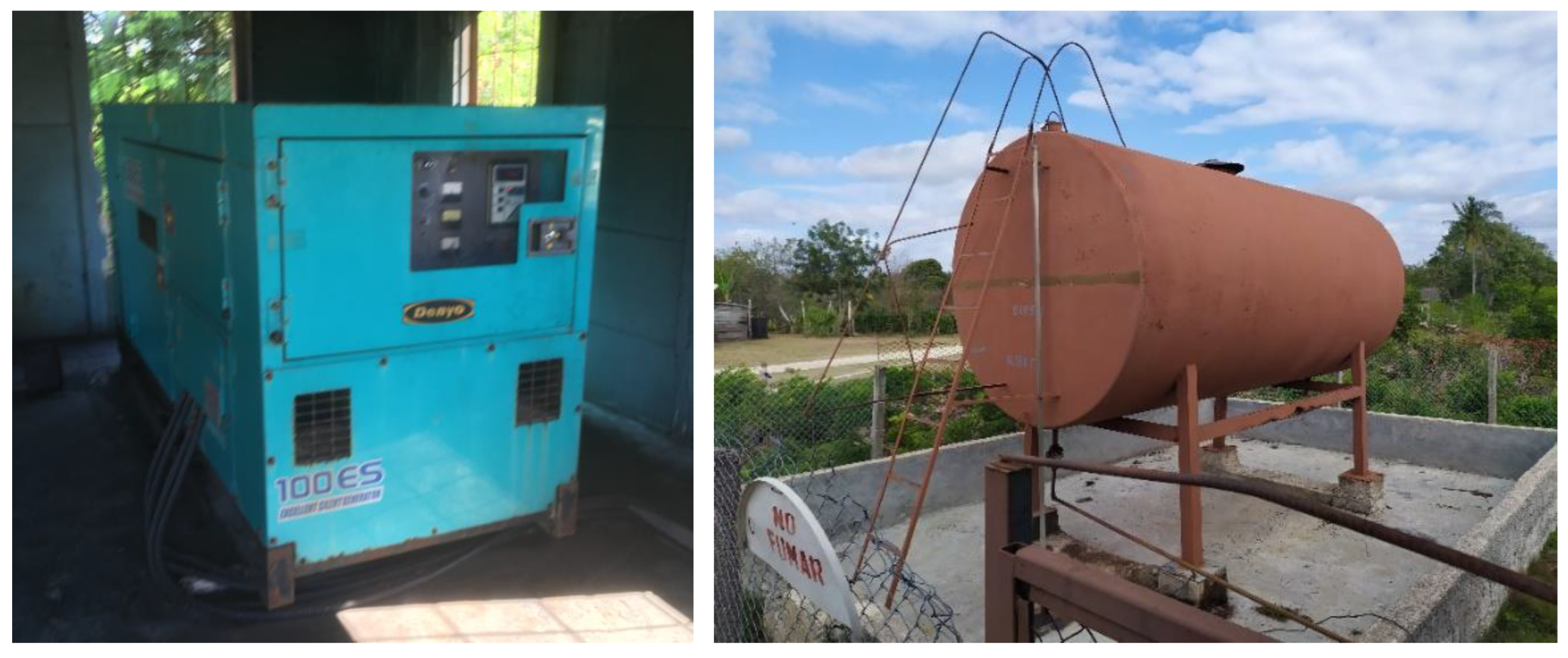
The diesel generator set is currently operative. With a power capacity of 80 kW, it results to be over-dimensioned for the actual maximum power consumption of the community[78]. The license plate specifications are reported in the Table 2:
Figure 4.
(left): The Engine-drive AC generator operating in Guasasa; (right): Diesel tank of the generator set in Guasasa (source: authors).
Figure 4.
(left): The Engine-drive AC generator operating in Guasasa; (right): Diesel tank of the generator set in Guasasa (source: authors).
3.2.2. Grid
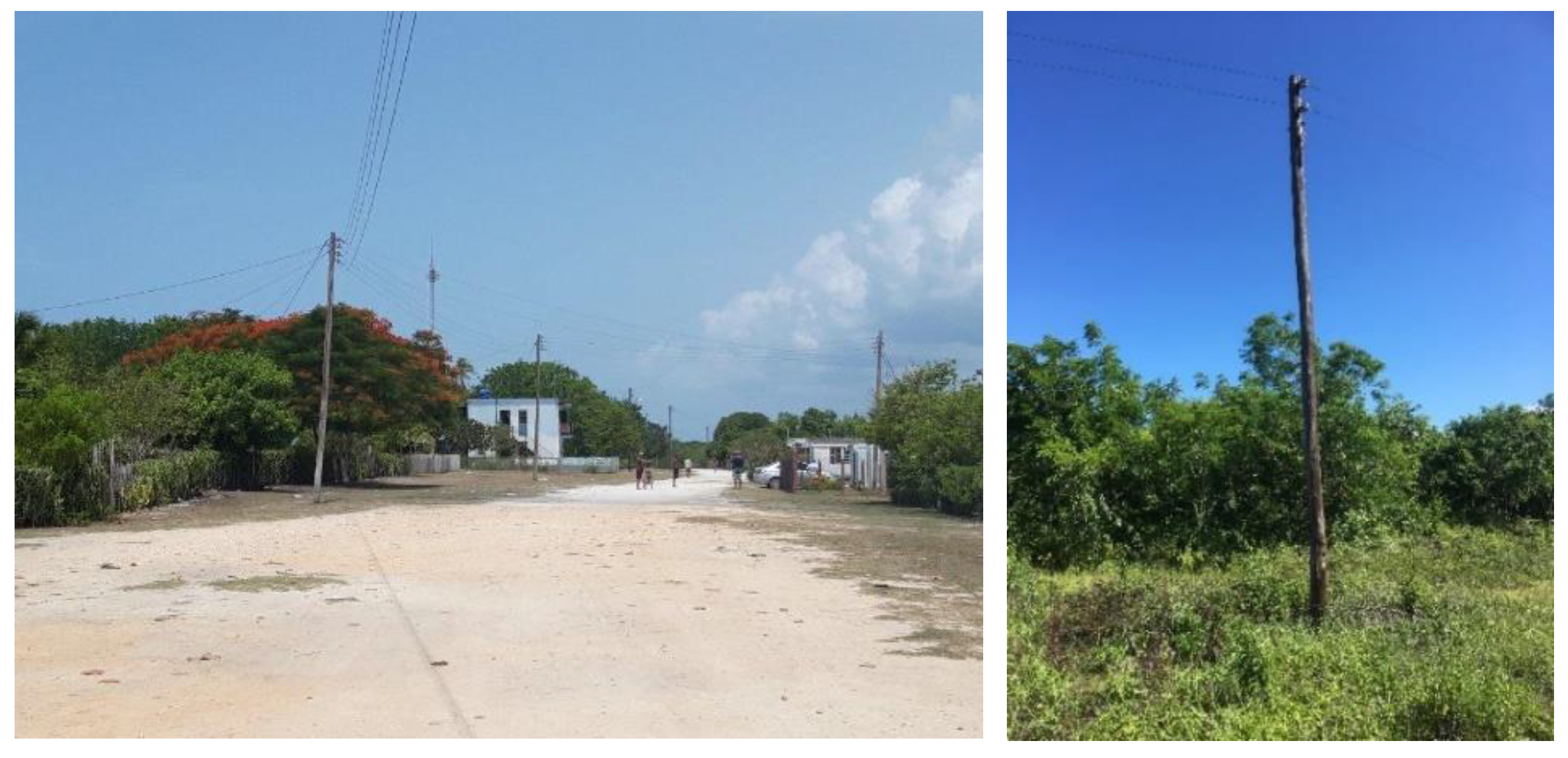
Guasasa is currently interconnected by a low voltage microgrid, isolated from the national transmission line. The main characteristics of the line are reported in the following table:
Table 3.
Characteristic of Guasasa grid.
| Low Voltage Line | |
|---|---|
| Voltage | 127/220 V (±10%) |
| Frequency | 60 Hz (±0.6 Hz) |
| Type | Three-phase (3F+N) Single-phase |
Figure 5.
(left): Three-phase grid; (right): Single-phase line, both in Guasasa (source: authors).
3.3. Energy demand
The energy demand in Guasasa is distributed in 95 buildings, including 85 houses, a medical center, pharmacy, school, cellar, canteen, refrigerator, video room, social center and water pump. CUBAENERGÍA studied the evolution of the daily energy demand using network analyzers for a week.
The current energy supply is limited to 12 hours a day divided into two periods: from 9 a.m. to 12 a.m. and from 3 p.m. to 12 p.m. Since the target is to achieve 24 hours a day of energy supply, the load of the remaining hours has been estimated. A constant demand was considered from 1 a.m. to 6 p.m., while from 1 p.m. to 3 p.m. and from 6 a.m. to 9 a.m. a linear growth was estimated. The resulting demand curve is therefore a combination of the average measurements and estimations for the uncovered periods.
Figure 6.
Daily demand curve of Guasasa obtained from network analysis [79].
Figure 6.
Daily demand curve of Guasasa obtained from network analysis [79].
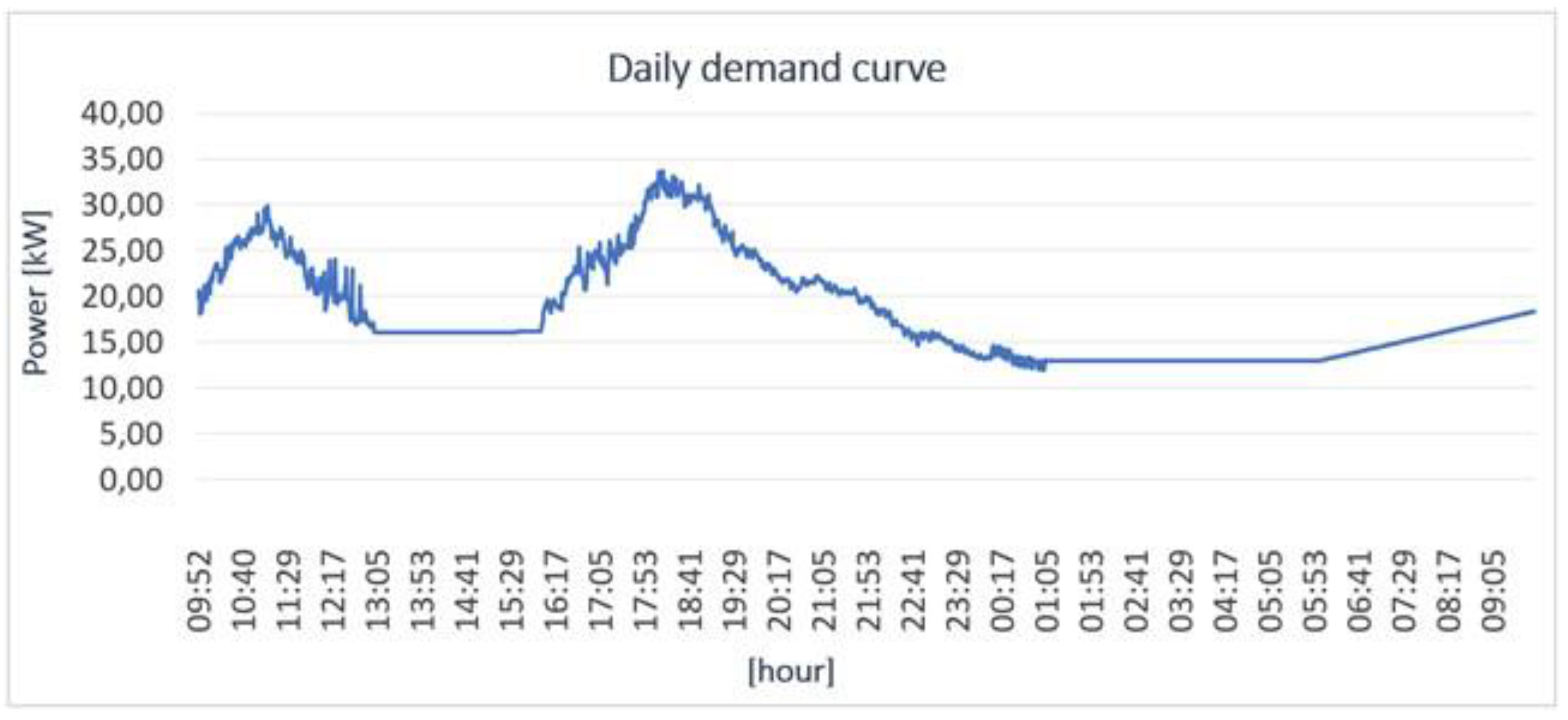
The diesel generator is the current power source with a daily production of 265 kWh. With these conditions, the daily planned energy production would be 545 kWh, so with a 25% of reserve respect the total estimated energy demand, equal to 437 kWh.
In Table 4, the main results derived from the network analysis are showed.
It is possible to calculate the average energy demand by extracting information from the daily energy load curve, hour by hour.
Figure 7.
Average hourly energy load for the community of Guasasa [73].
Figure 7.
Average hourly energy load for the community of Guasasa [73].
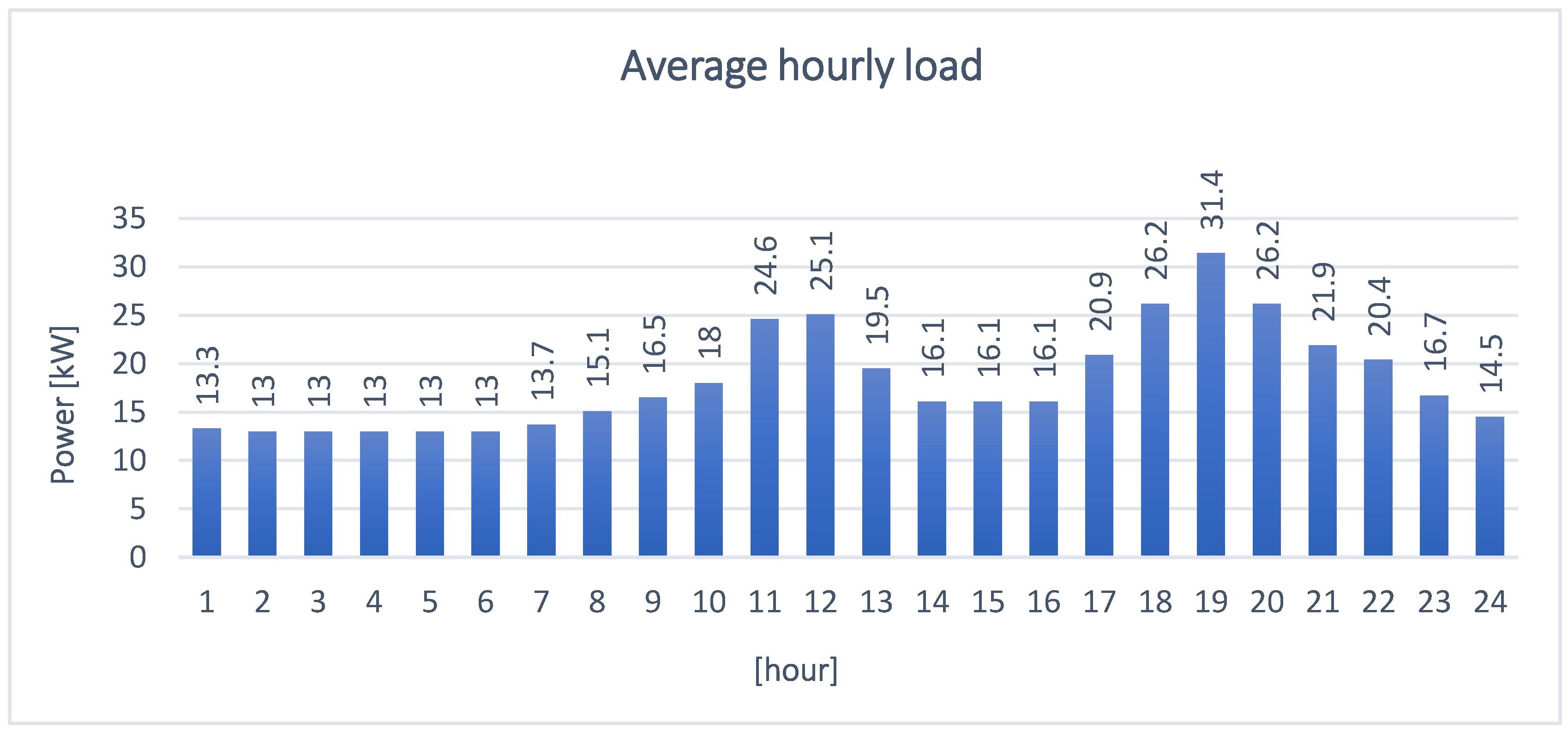
Some useful parameters can be derived from this study. Knowing the value of the peak load (=34 kW) and calculating the average daily load (=18.2 kW), the load factor () can be calculated:
3.3.1. Allocation
One of the advantages of using GIS technologies in electrification planning is the possibility to consider the spatial variability effect of the energy demand.
Especially for the comparison of individual cases or different groups of microgrids, the right amount distribution of energy demand to each single load can have a significant effect on techno-economical assessments. In this study case, the only available information about the specific type of loads is the power of the public water pump (), located in the northern part of the community.
All the other types of loads have been differentiated by distributing the total energy demand and the peak load. In this process, different weights have been assigned depending on the common usage of each type of facility.
Figure 8.
Satellite view of the areas of Guasasa characterized by different type of buildings (Source: Google Maps; [73]).
Figure 8.
Satellite view of the areas of Guasasa characterized by different type of buildings (Source: Google Maps; [73]).
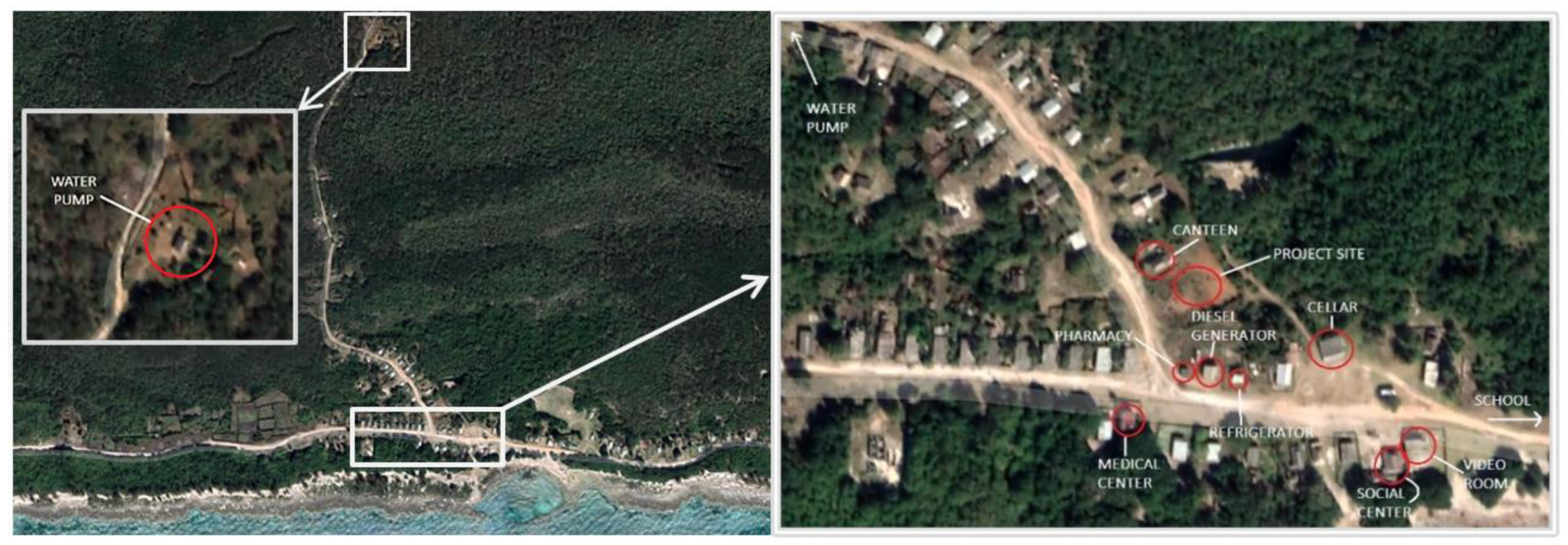
The estimated peak load is 34 kW and refers to the aggregated peak load (Ppeak,aggr) of the community. By assigning a proper coincidence factor (), we can calculate the total Ppeak,tot) that is the sum of the individual peak loads (Ppeak,i) and then allocate the peak power of every facility.
Knowing the total daily energy demand and the sum of the peak load of each single facility, it is possible to complete the demand allocation as reported in the Table below.
Table 5.
Daily energy demand and peak power allocation between the different types of facilities in Guasasa [73].
Table 5.
Daily energy demand and peak power allocation between the different types of facilities in Guasasa [73].
| Building | n | [kWh/day] | [kWh/day] | [kW] | [kW] | [kW] | |
|---|---|---|---|---|---|---|---|
| House | 85 | 4.5 | 383.2 | 0.9 | 75.8 | 0.4 | 34 |
| Medical center | 1 | 4.5 | 4.5 | 0.9 | 0.9 | ||
| Pharmacy | 1 | 2.3 | 2.3 | 0.4 | 0.4 | ||
| School | 1 | 4.5 | 4.5 | 0.9 | 0.9 | ||
| Cellar | 1 | 4.5 | 4.5 | 0.9 | 0.9 | ||
| Canteen | 1 | 4.5 | 4.5 | 0.9 | 0.9 | ||
| Refrigerator | 1 | 6.8 | 6.8 | 1.3 | 1.3 | ||
| Video room | 1 | 2.3 | 2.3 | 0.4 | 0.4 | ||
| Social center | 1 | 4.5 | 4.5 | 0.9 | 0.9 | ||
| Water pump | 1 | 20.0 | 20.0 | 2.5 | 2.5 | ||
| Total | 94 | 437.0 | 85.0 |
3.4. Input Assumptions
All the techno-economic assumptions have been defined according to previous studies performed with similar analysis, technological state and experimental values.
An important economic index required by the model is the discount rate, from which the capital recovery factor is derived (equation 35). For the action, a nominal discount rate of 8.9% is detected [74]. Since an increase is expected in Cuba during the period 2016 – 2033 [80], the present study considers a value of 10% for the nominal discount rate (). However, the parameter used for the LEC assessment is the real discount rate (), obtainable from and the inflation rate ():
The resulting value is a real discount rate of 7%.
Table 6.
Indexes used for the economic assessment in Guasasa.
| ECONOMIC INDEXES | |
|---|---|
| Nominal Discount Rate | 10% |
| Inflation Rate | 2.8% |
| Real Discount Rate | 7% |
All the cost assumptions have been converted from United States Dollars to Euros by a conversion rate of: $/€ = 0.89.
3.4.1. PV Modules
For the PV generation performance characterization, a lifetime of 25 years has been considered. A lower global efficiency (Performance Ratio) is determined for the stand-alone PV system whereas for the Centralized system, the value used for the global efficiency was: 80%.
The capital expenditure for the solar modules estimated is equal to 1557 €/kW. The National Renewable Energy laboratory at US (NREL) proposes the following module prices valid for the USA, distinguishing between residential and commercial scale [81]:
- Overnight capital cost for residential scale (< 10 kW): 2235 €/kW;
- Overnight capital cost for commercial scale (> 10 kW): 1425 €/kW.
In this case, is considered the same proportion between residential and commercial scale to calculate the capital cost of a stand-alone module in Guasasa, obtaining the following result: 1557 €/kW. Hence, the Investment costs considered for the execution of the model are:
- Stand-alone system investment cost: 2443 €/kW;
- Centralized system investment cost: 1557.5 €/kW.
For the annual Operation & Maintenance costs, the same source was considered:
- Stand-alone system O&M costs: 17.8 €/kW;
- Centralized system O&M costs: 14.2 €/kW.
The input settings related to the solar systems are listed in the following table.
Table 7.
Input settings for a PV stand-alone system.
| Type | Ipv [€/kWp] | OMpv[€/kWp] | pv |
|---|---|---|---|
| Stand-alone | 2443 | 18 | 65% |
| Centralized | 1558 | 14 | 80% |
3.4.2. Diesel
The International Renewable Energy Agency (IRENA) [82] proposes the following range for the price of a diesel generation set: 200 €/kW < ID < 600 €/kW. As an average value in the suggested range, the capital expenditure considered for the case study of Guasasa is: ID = 400 €/kW.
For the cost of O&M, a value of 0.02 € for each hour of operation and per units of power size of the diesel generator is chosen: OMD = 0.02 € (hoperation∙kW).
Due to shortage of supply for the isolated location, the diesel price is particularly high: 48 CUP/l, equal to 1.78 €/l. From the consumption analysis of the actual generator set, a value of 0.4 l/kWh is detected for the fuel consumption.
- Fuel price: Fp = 1.78 €/l;
- Fuel consumption: COF = 0.4 l/kWh.
As design factor of the electric machine, a higher value than the coincidence factor of the loads is taken, for reasons of security margin:
- Design factor: = 0.77.
The expected lifetime is 20 years ( 20), while major maintenances is estimated to be needed every 5 years (5).
The input settings related to the diesel generator set are listed in the following table.
Table 8.
Input settings for the diesel generator set.
| nD | nrec | ID [€/kW] | OMD [€/(hop·kW)] | Fp [€/l] | COF [l/kWh] | |
|---|---|---|---|---|---|---|
| 20 | 5 | 400 | 0.02 | 0.77 | 1.78 | 0.40 |
3.4.3. Storage
For the storage performance characterization, a round-trip energy efficiency of 85% and, according with HOMER data [83], an optimal lifetime of 18 years has been used, along with a 70% depth of discharge.
The reference cost considered for the storage in Guasasa is 179.4 €/kWh. The annual O&M costs considered are 4.1 €/kWh.
For the PV systems, the days of autonomy should be enough to guarantee the desired reliability, covering the maximum estimated strings of consecutive non-solar days. A value of 3 days is used both for the individual and the centralized case. For a hybrid system, the reliability is guaranteed by the diesel generator, so the storage capacity can be lower. Two hybrid configurations will be tested in the next paragraph for different percentage of renewable fraction. For the hybrid system with 50% of renewable fraction, 1 day of battery autonomy is considered sufficient. For the hybrid system with 75% of renewable fraction, the intervention of the diesel generator needs to be limited, so 2 days of battery autonomy are set. Due to the modular nature of batteries, no distinctions are considered between the costs of individual and centralized systems. The remaining technical parameters are taken from Table 9, where the input settings related to storage are listed.
3.4.4. Power Conditioning
For the power conditioning performance characterization, an efficiency of 95% and a lifetime of 15 years have been selected.
For the economic characterization, the same investment cost ( is associated for the individual and the centralized case. However, the greater complexity of the centralized system is taken into account by the next correction factor:
Ipc,ind = Ipc,centr = 267 €/kW
No Operation & Maintenance costs are considered. The remaining technical parameters are taken from Table 9.
The input settings related to power conditioning storage are listed in the following table:
Table 10.
Input settings for the power conditioning.
| npc | Ipc [€/kW] | OMpc [€/kW] | inv,pv |
|---|---|---|---|
| 15 | 267 | 0 | 95% |
3.4.5. Grid
The grid which is actually operating in Guasasa is a low voltage system. For the hypothetical condition of complete electrification, only the low voltage line investment is implemented in the model, considering the small distances to be covered.
Louie proposes the following range of construction costs for a low voltage distribution line in isolated areas: 8900 €/km < ILV < 16000 €/km [31]. The line costs per unit of distance tends to increase for smaller grids, due to the effect of fixed costs, so the highest value of the range suggested is considered: ILV = 16000 €/km.
The annual O&M costs are assumed as 1% of the capital cost: OMLV = 160 €/km. As costs of connection, a value of 100 €/kW is defined. The expected lifetime is 30 years.
The input settings related to the grid are listed in the following table:
Table 11.
Input settings for the distribution line and connection system.
| nLV | ILV [€/km] | OMLV[€/km] | ICN [€/kW] |
|---|---|---|---|
| 30 | 16000 | 160 | 100 |
3.5. Model Test
Once defined all the inputs, the model can be tested. Five layers of GIS data are required, as introduced in Section 2.2:
- Point layer of the whole community. Each point represents a building and is characterized by an attribute Table reporting all the techno-economic assumption and the load energy demand previously discussed (Figure 9 left);
- Point layer of the group of buildings to be networked in a microgrid. It is obtained as a selection of the point layer of the whole community, so it is characterized by the same attribute Table (Figure 9 right);
- Line layer of the central distribution line supposed for the ideal case of complete electrification needed (Figure 9 left);
- Digital Surface Model of Guasasa, with a resolution of 30x30 meters (Figure 10);
- Global solar radiation raster on optimal angle tilted surface, with a high spatial resolution (30x30 m) (Figure 11).
The type of configuration is determined by the group of buildings selection in the second point layer. In general, three cases can be simulated:
- All the buildings selected: centralized system to feed the whole community;
- No selection: all the buildings supplied by stand-alone PV systems;
- A group of buildings selected: selected buildings fed by the microgrid, while the remaining are supplied by stand-alone PV systems.
Introducing the group of buildings (points) to be centralized, the model automatically selects the area in their surrounding and properly extract the portion of distribution line needed for the microgrid.
Three different conditions will be considered in the model execution:
- Total centralized case: a complete electrification is needed. The ideal starting point considered is a total absence of power generation and distribution facilities;
- Partial case: same hypothetical condition of the first case but a combination of the centralized and the individual solution is considered (stand-alone + centralized);
- Real case: The starting point considered is the actual level of electrification in Guasasa and the actual facilities are kept.
For each of the three conditions, all the available types of power plant implemented will be investigated, always assuming the target of 24 hours/day of energy supply for the whole community. Note that a specific location in the map is considered for the numerical results reported in the following section. For the case of the centralized systems it corresponds to the planned location, visible in Figure 8. Anyway, information about the resulting LEC of a power plant located in any other area is provided by a graphical representation. Similarly, to simplify the review, the numerical results of only one building is considered for the individual systems. The choice falls on the isolated house in the extreme south east of the village.
In the results visualization, the weight of each subsystem in the total cost per kWh is displayed in different colors. The category “Grid” includes the sum of the line and the connection costs.
3.5.1. PV stand-alone
The first run is related to a stand-alone photovoltaic system for every building. The calculation for the chosen reference house produced the results reported in Table 12.
A LEC of 21 €cents/kWh was obtained. As can be noticed by the diagram of the cost contributions, the storage system results the subsystem that affects the most the total costs.
Figure 12.
Cost contribution of each subsystem to the total LEC of a PV stand-alone system in Guasasa.
Figure 12.
Cost contribution of each subsystem to the total LEC of a PV stand-alone system in Guasasa.
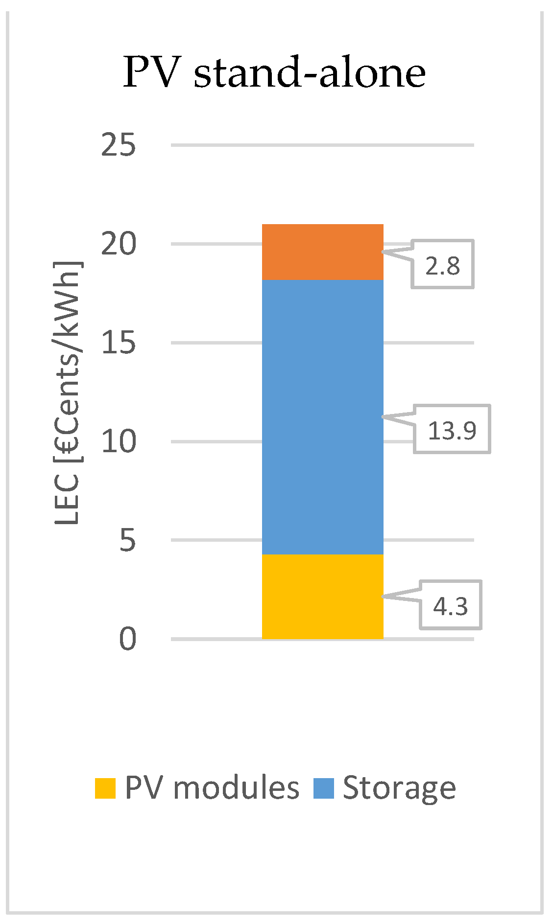
The incoming solar radiation is very uniform along the whole study area, due to morphological characteristics (substantially flat) and the absence of shading obstacles. As a consequence, both the capacity factor and the LEC obtained for each individual power plant have a homogeneous distribution.
In the Figure below, the LEC obtained for a PV stand-alone system installed to supply the demand of each building of the community.
Figure 13.
LEC of the PV stand-alone systems required to feed each energy load of Guasasa.
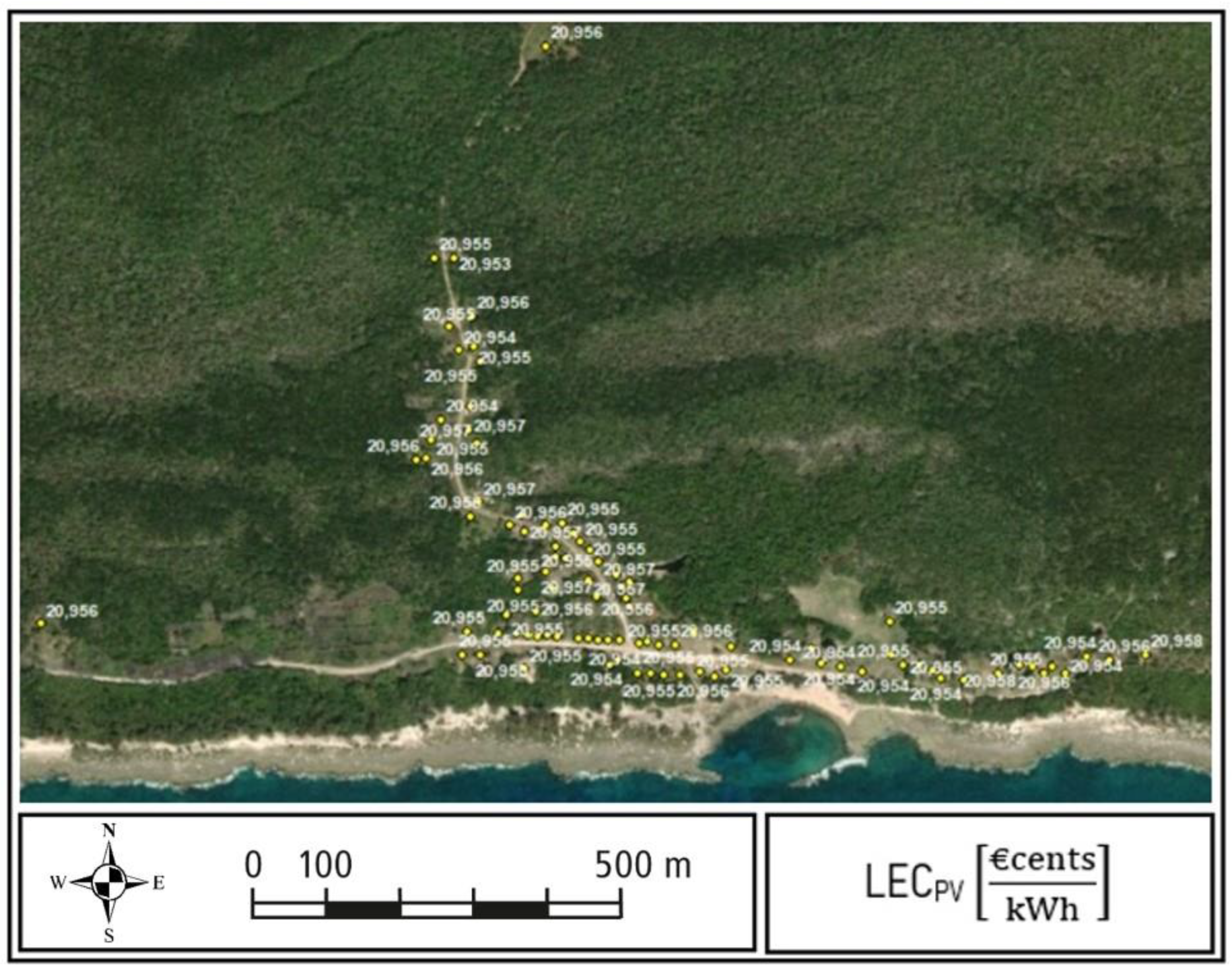
As it can be noticed, the variation between different values is negligible, but it is present. It means that in a condition of higher spatial fluctuation of the available resource, the differences would be more evident and would provide more useful information to the user.
3.5.2. PV Centralized
The model execution for the centralized cases includes three runs, corresponding to the previously introduced scenarios. The first (total) and second (partial) cases use the same inputs for the centralized PV system, as both start from a condition with no existing electrification equipment. However, the partial case additionally incorporates inputs for stand-alone systems, since the excluded loads from the centralization perform individual LEC calculations simultaneously. The third run represents the real case, where the distribution system is already operational, resulting in zero investment costs for the low voltage distribution line and connection costs.
A summary of the results of the model execution for the three cases is reported in the Table 13.
In Figure 14, the cost contribution of each subsystem in the three cases tested are showed.
3.5.3. Hybrid Diesel-PV 75%
The first hybrid Diesel-PV power plant considered has a renewable fraction of 75%. The input settings follow the same conditions as the three previous cases, adding the parameters relative to the diesel generator and the fuel costs. For the real case, no investment costs are defined for the diesel generator, which is currently operative in Guasasa.
A summary of the results of the model execution for the three cases is reported in the Table 14.
The resulting LEC obtained for each case is respectively: 38.8 €cents/kWh, 38.6 €cents/kWh and 36.1 €cents/kWh. In addition to the decrease of the line costs, with the same trend presented in the previous paragraph, a reduction can be noticed in the diesel subsystem. Between the ideal cases and the real one, the costs associated to the diesel generator decrease, since in the last case only the operation and maintenance expenditures are considered.
In Figure 15, the cost contribution of each subsystem in the three cases tested are showed.
3.5.4. Hybrid Diesel-PV 50%
The important setting change in the hybrid system passing from one configuration to the other is the battery autonomy. As previously motivated, one day of autonomy is considered sufficient for the reliability of a diesel-PV system with 50% of renewable fraction, rather than the two days set for the 75% case.
A summary of the results of the model execution for the three cases is reported in the Table 15.
The resulting LEC obtained for each case is respectively: 51.0 €cents/kWh, 50.8 €cents/kWh and 49.2 €cents/kWh. The observations derivable by the comparison of the three cases are the same encountered in the other hybrid system: a decrease of the line costs and of the diesel generator costs. The comparison between the two hybrid systems ( 75% and 50%) is more significant. As expected, in this last case the storage costs decrease, while the fuel costs increase, since the diesel contribution in the energy generation balance is doubled. The increase of the capacity factor implies a decrease of the diesel subsystem cost. Overall, the raise prevails, leading to a higher total LEC value.
In Figure 16, the cost contribution of each subsystem in the three cases tested are showed.
3.5.5. Diesel Generator Set
The last type of configuration considered is a diesel generator set that directly feeds all the energy demand considered, without any storage or external power conditioning system. In particular, the real case represents an increase of the diesel generator set use from the actual 12 hours/day of operation to a continuous operation.
A summary of the results of the model execution for the three cases is reported in the Table 16.
The resulting LEC obtained for each case is respectively: 75.0 €cents/kWh, 74.8 €cents/kWh and 73.7 €cents/kWh. Despite the absence of several cost contributors and a most efficient use of the diesel generator, the total LEC appears to be the highest in all the three cases. It is evident that the cause is the high cost associated to the fuel consumption. Even omitting any environmental issues, the present investigation, with the assumption made, identifies the diesel generator set as the least cost-effective solution for the case study. In addition, the country's special conditions for accessing fuel should be considered.
In Figure 17, the cost contribution of each subsystem in the three cases tested are showed.
3.5.6. Maps Output
The main potential of the model is its maps result. For every configuration and case tested, the raster format allows a second level of analysis, which shows the variation of the resulting LEC in terms of placement of the centralized system.
We can focus on the graphical output of the Hybrid Diesel-PV system configuration with a renewable fraction of 75%, again for the three cases: total, partial and real.
Figure 18 reports the resulting raster representation of the LEC obtained for the total case.
This case refers to a full centralization, including all the buildings as part of the hybrid system and without considering the existing level of electrification in Guasasa. It is evident that the LEC decreases in proximity to the central distribution line represented in Figure 19. The grid costs prevail over the spatial fluctuations in the PV system cost, which are negligible due to the uniform distribution of solar radiation in this area.
Figure 19 reports the resulting raster representation of the LEC obtained for the partial case.
We consider as partial centralization a mixed system including the group of building highlighted from Figure 19 in a centralized system and the rest of the building supplied by PV stand-alone systems. The same considerations outlined for the total case may be observed for the partial case. An important feature is the possibility to visualize both the centralized and the individual option in the same map. The LEC values calculated for the stand-alone systems appear over each building, likewise in the case of total individual configuration (Figure 13).
The last simulation considered is the base case scenario where the hybrid system is an integration of the existing diesel generator and grid. Since the buildings are actually connected by the distribution line, the real case refers to a fully centralized system. The resulting LEC is represented in Figure 20.
3.6. Results Comparison
The proposed approach by this new model enables the assessment of various configurations on multiple levels of comparison.
The differences revealed by the comparison of three cases could be significant in a different context. The limited size of the study area is reflected in a low impact of the distribution line costs, which would increase considerably if higher voltage systems were required. Also, the size of the required power plants does not justify a possible cost variation due to economies of scale, as it is the case between the stand-alone and the centralized solar system. In case of higher powers involved, the transition from a complete centralization to various configurations of microgrids would have a more evident effect on cost evaluation.
The characteristic and size of the study areas do not involve sensible fluctuation of the solar resource from a spatial point of view. For this reason, the information about the best installation site location for a centralized system (provided by the raster format of the LEC) results to be mainly driven by the distance from the line, which has a low impact. Integrating the hybrid model with other types of renewable-based power plant would increase the spatial variability of the available resources. This would take the most advantage from the versatility of the IntiGIS-local model created as a decision-making instrument. Another effective comparison that deserves a closer look is between the different types of power generation systems investigated.
The LEC of the two configurations of the solar systems appears to be mainly equal. The lower cost per kWh associated to the solar panel of the centralized system are balanced by the higher cost of the power conditioning and by the cost associated to the grid. From the PV centralized system to the diesel generator set and the two types of hybrid system, the same trend can be noticed. The higher the renewable fraction, the more the storage and diesel generator costs increase, while fuel consumption decreases. The storage costs are related to the required reliability of the power plant. The diesel generator costs depend on its capacity factor. Since its size is fixed by the total energy demand, an increase of contribution in the total energy production clearly leads to a lower associated cost per kWh produced. The weight assumed by each of the subsystems involved determine the overall evolution of this trend. In this case study, the fuel subsystem results to have a very high impact in the total cost. It is justified by the high price of the diesel considered, motivated by the isolated location of Guasasa. It can be noticed that a lower fuel price would definitely increase the competitiveness of the hybrid system as electrification option. The trend is evident in all the three cases previously investigated. The following paragraph will further highlight the comparison between the different configurations.
3.6.1. Total Centralization
3.6.2. Partial Centralization
In the Table 18 and Figure 22, the LEC comparison among the different types of power plant and the contribution of each subsystem cost is investigated. The case considered is the partial centralization, starting from the ideal condition of absence of any electrification equipment. The loads excluded by the centralized system are considered supplied by a PV stand-alone system.
3.6.3. Real Case
In the Table 19 and Figure 23, the LEC comparison among the different types of power plant and the contribution of each subsystem cost investigated. The case considered is the actual electrification condition in Guasasa.
The discussion and contextualization of these results is the subject of the following section.
4. Discussion
This paper describes a whole methodology, based on GIS models, and developed to aid in the deployment of rural electrification with renewable energy technologies. When designing an electrification plan for a large region, regional GIS-based, as described in the literature, often rely on simplifying assumptions in order to expedite computation speeds. However, the proposal of the present investigation, operates at a building-level, enabling more precise calculations for smaller areas of interest.
IntiGIS-local empowers designers to choose from various technologies and configurations based on comprehensive GIS-formatted information, including social, techno-economic and geographical factors. This approach allows the analysis of communities or study areas, considering combinations of electrification alternatives, such as individual systems and micro-grids. In contrast, with other GIS models that only consider the cost of connecting an entire community or grid cell with a single technology. Even LREM, which operates at local scale and at a building level, assumes that all buildings in a defined area should be connected to a single microgrid system.
Furthermore, models that connect entire communities or grid cells with a single technology, face challenges in estimating the cost of distribution infrastructure. Some models estimate or assume these costs based on the mean distance between households, generating the total length of required distribution infrastructure. To calculate transmission costs, they typically assume the need for building transmission infrastructure to the center of the cell or community. Concerning to this issue, IntiGIS-local calculates all possible installation sites for centralized power plants within the polygon representing the reference area of the centralized system. This approach enables the visualization of the variation in the resulting LEC raster format, depending on the placement of the centralized system. Such flexibility provides valuable insights for users in making informed decisions regarding the optimal placement of centralized systems.
The methodology has been successfully implemented into an ArcGIS tools and applied in a real case study. As previously discussed, the results from the case study reveal few differences in terms of PV technology in the three analyzed scenarios. In all cases, the use of solar technology is clearly competitive with the incorporation of a diesel unit, largely due to the higher fuel costs. It's noteworthy that such competitiveness may vary across countries and locations, influenced by factors such as fuel subsidization or complex supply logistics, as observed in the preexisting literature. In addition to these aspects, we should consider elements such as insecurity or corruption or, as in the Cuban case, the intermittency in the supply chains.
Moreover, given the small difference in the LEC, other aspects such as the availability of space or management capacity can be decisive when deciding between an individual photovoltaic system and a small microgrid plant. Likewise, maintenance and the cost per energy consumed policy will be key elements to take into account in the final decision.
Beyond the specific results of the Guasasa case study, the proposed methodology and the geographic model built on it bring great opportunities for its use in the rural electrification field, confirming in this way that the versatility of the development of geographic models such as the one we propose is widely proven.
As we explained in the methodology section, the study of the LEC as a valuable method for intercomparing isolated electrification systems have a long history. The work presented here is an important milestone in this line, since it allows the comparison between two very frequent options in rural electrification: the use of individual photovoltaic systems versus hybrid microgrids, combining a small photovoltaic plant and a diesel generator. The ability to contrast these options, especially in locations with diverse demands, schedules, and uses, adds a nuanced perspective to the discussion.
Author Contributions
JD Direction of the research. Conceptualization, J.D., L.A. and J.A.; methodology, J.D., M.T., A.M. and C.B.; software and validation, C.B., A.M. and M.T.; writing—original draft preparation, C.B. and J.D.; all the authors writing—review and editing; scientific supervision, J.D., J.A. and L.A.; project administration, J.D.; funding acquisition, J.D.
Funding
This research was funded by Spanish Agency for International Development Cooperation (AECID), grant number 2018/ACDE/000600, under the innovation action HIBRI2, and by the ERASMUS + program of the European Union (I-PADOVA01).
Acknowledgments
We would express our recognition to the fundamental work at HIBRI2 project of the Cuban Center for Information Management and Energy Development (CUBAENERGÍA) as well as the NGO Cuban Society for the Promotion of Renewable Energy Sources and Respect for the Environment (CUBASOLAR). A special acknowledge to the people of Guasasa and the municipality's authorities.
Conflicts of Interest
The authors declare no conflict of interest.
References
- IEA. World Energy Outlook 2019; International Energy Agency: 2019; p. 690.
- IEA. World Energy Outlook 2020; International Energy Agency: 2020.
- Fu, M.; Shen, H. COVID-19 and Corporate Performance in the Energy Industry. Energy RESEARCH LETTERS 2020, 1. [CrossRef]
- Śleszyński, P.; Nowak, M.; Brelik, A.; Mickiewicz, B.; Oleszczyk, N. Planning and settlement conditions for the development of renewable energy sources in poland: Conclusions for local and regional policy. Energies 2021, 14, 1935. [CrossRef]
- Qv, D.; Duan, X.; Wang, J.; Hou, C.; Wang, G.; Zhou, F.; Li, S. Issues and Potential Solutions to the Clean Heating Project in Rural Gansu. Sustainability 2021, 13, 8397. [CrossRef]
- Gershon, O.; Emekalam, P. Determinants of Renewable Energy Consumption in Nigeria: A Toda Yamamoto Approach. In Proceedings of the IOP Conference Series: Earth and Environmental Science, 2021; p. 012005.
- Bose, D.; Saini, D.K.; Yadav, M.; Shrivastava, S.; Parashar, N. Review of Sustainable Grid-Independent Renewable Energy Access in Remote Communities of India. Integrated Environmental Assessment and Management 2021, 17, 364-375. [CrossRef]
- Bose, D.; Saini, D.K.; Yadav, M.; Shrivastava, S.; Parashar, N. Decentralized Solar Energy Access and Assessment of Performance Parameters for Rural Communities in India. Sustainability and Climate Change 2021, 14, 103-114. [CrossRef]
- Shen, H.; Shen, G.; Chen, Y.; Russell, A.G.; Hu, Y.; Duan, X.; Meng, W.; Xu, Y.; Yun, X.; Lyu, B. Increased air pollution exposure among the Chinese population during the national quarantine in 2020. Nature Human Behaviour 2021, 5, 239-246. [CrossRef]
- Sambodo, M.T.; Fuady, A.H.; Negara, S.D.; Handoyo, F.W.; Mychelisda, E. Epilogue: Agenda for Development of Rural Electrification. In Electricity Access and Community Welfare in Indonesia; Springer: 2021; pp. 69-89.
- Ringler, C.; Alqarawy, A.M.; Brent, W.; Collins, G.; Orengoh, P.; Scanlon, B.; Yaseen, L. Enhanced water security and energy access: Key investments for Sub Saharan Africa; 2020. https://hdl.handle.net/10568/114228.
- Otieno, J.; Otieno, A. Adoption of Clay Charcoal Briquetting to Curb Deforestation and the Impacts of Covid-19 Pandemic in Rural Areas, Kenya. European Journal of Environment and Earth Sciences 2020, 1. [CrossRef]
- Osabuohien, E.S.; Ejemeyovwi, J.O.; Ihayere, O.B.; Gitau, C.M.; Oyebola, F.M. Post-Pandemic Renewable Energy Development in Sub-Saharan Africa. Sustainability and Climate Change 2021, 14, 183-192. [CrossRef]
- Liu, X.; Wu, Y.; Liu, J.; Liao, Z. Re-Exploration of the Sustainability of Traditional Village Spatial Development in The Epidemic Era–From the Perspective of Jiangnan Region, China. In Proceedings of the E3S Web of Conferences, 2021; p. 04009.
- Ghenai, C.; Bettayeb, M. Data analysis of the electricity generation mix for clean energy transition during COVID-19 lockdowns. Energy Sources, Part A: Recovery, Utilization, and Environmental Effects 2021, 1-21. [CrossRef]
- Du, S.; Liu, J.; Fu, Z. The Impact of Village Rules and Formal Environmental Regulations on Farmers’ Cleaner Production Behavior: New Evidence from China. International Journal of Environmental Research and Public Health 2021, 18, 7311. [CrossRef]
- Chaudhary, M.K.; Dhakal, A.P. COVID-19 Pandemic and its Impact on Sustainable Development Goals: An Observation of South Asian Perspective. Annals of the Romanian Society for Cell Biology 2021, 01-14.
- Lin, X.-M.; Kireeva, N.; Timoshin, A.V.; Naderipour, A.; Abdul-Malek, Z.; Kamyab, H. A multi-criteria framework for designing of stand-alone and grid-connected photovoltaic, wind, battery clean energy system considering reliability and economic assessment. Energy 2021, 224, 120154. [CrossRef]
- Nagaj, R.; Korpysa, J. Impact of COVID-19 on the Level of Energy Poverty in Poland. Energies 2020, 13. [CrossRef]
- Sueyoshi, T.; Ryu, Y.; Yun, J.-Y. COVID-19 Response and Prospects of Clean/Sustainable Energy Transition in Industrial Nations: New Environmental Assessment. Energies 2021, 14. [CrossRef]
- Bompard, E.; Mosca, C.; Colella, P.; Antonopoulos, G.; Fulli, G.; Masera, M.; Poncela-Blanco, M.; Vitiello, S. The Immediate Impacts of COVID-19 on European Electricity Systems: A First Assessment and Lessons Learned. Energies 2021, 14. [CrossRef]
- Navon, A.; Machlev, R.; Carmon, D.; Onile, A.E.; Belikov, J.; Levron, Y. Effects of the COVID-19 Pandemic on Energy Systems and Electric Power Grids—A Review of the Challenges Ahead. Energies 2021, 14. [CrossRef]
- Kirli, D.; Parzen, M.; Kiprakis, A. Impact of the COVID-19 Lockdown on the Electricity System of Great Britain: A Study on Energy Demand, Generation, Pricing and Grid Stability. Energies 2021, 14. [CrossRef]
- Maniatis, K.; Chiaramonti, D.; van den Heuvel, E. Post COVID-19 Recovery and 2050 Climate Change Targets: Changing the Emphasis from Promotion of Renewables to Mandated Curtailment of Fossil Fuels in the EU Policies. Energies 2021, 14. [CrossRef]
- Kolosok, S.; Bilan, Y.; Vasylieva, T.; Wojciechowski, A.; Morawski, M. A Scoping Review of Renewable Energy, Sustainability and the Environment. Energies 2021, 14. [CrossRef]
- Energy - United Nations Sustainable Debelopment. Available online: https://www.un.org/sustainabledevelopment/energy/ (accessed on 23 Septembre 2021).
- Mostofi, F.; Shayeghi, H. Feasibility and optimal reliable design of renewable hybrid energy system for rural electrification in Iran. International Journal of Renewable Energy Research (IJRER) 2012, 2, 574-582. [CrossRef]
- Elkadeem, M.R.; Younes, A.; Sharshir, S.W.; Campana, P.E.; Wang, S. Sustainable siting and design optimization of hybrid renewable energy system: A geospatial multi-criteria analysis. Appl Energ 2021, 295, 117071. [CrossRef]
- Bekele, G.; Tadesse, G. Feasibility study of small Hydro/PV/Wind hybrid system for off-grid rural electrification in Ethiopia. Appl Energ 2012, 97, 10. [CrossRef]
- Angelis-Dimakis, A.; Biberacher, M.; Dominguez, J.; Fiorese, G.; Gadocha, S.; Gnansounou, E.; Guariso, G.; Kartalidis, A.; Panichelli, L.; Pinedo, I.; et al. Methods and tools to evaluate the availability of renewable energy sources. Renew Sustain Energy Rev 2011, 15, 1182-1200. [CrossRef]
- Louie, H. Off-Grid Electrical Systems in Developing Countries; Springer International Publishing: 2018.
- Nerini, F.F.; Broad, O.; Mentis, D.; Welsch, M.; Bazilian, M.; Howells, M. A cost comparison of technology approaches for improving access to electricity services. Energy 2016, 95, 255-265. [CrossRef]
- Chaurey, A.; Kandpal, T.C. Assessment and evaluation of PV based decentralized rural electrification: An overview. Renew Sustain Energy Rev 2010, 14, 2266-2278. [CrossRef]
- Barnes, D.F. The challenge of rural electrification: strategies for developing countries; Earthscan: 2010.
- Nässén, J.; Evertsson, J.; Andersson, B.A. Distributed power generation versus grid extension: an assessment of solar photovoltaics for rural electrification in Northern Ghana. Prog. Photovolt: Res. Appl. 2002, 10, 495-510.
- Domínguez Bravo, J. Los sistemas de información geográfica en la planificación e integración de energías renovables; CIEMAT: Madrid, 2002; p. 159.
- Dugoua, E.; Kennedy, R.; Urpelainen, J. Satellite data for the social sciences: measuring rural electrification with night-time lights. International journal of remote sensing 2018, 39, 2690-2701.
- Monteiro, C.; Saraiva, J.T.; Miranda, V. Evaluation of electrification alternatives in developing countries - The SOLARGIS tool. In Melecon '98 - 9th Mediterranean Electrotechnical Conference, Vols 1 and 2; Ieee Conference Record; 1998; Volume 2, pp. 1037-1041.
- Amador, J.; Dominguez, J. Application of geographical information systems to rural electrification with renewable energy sources. Renew Energy 2005, 30, 1897-1912. [CrossRef]
- Domínguez Bravo, J.; Amador, J. Geographical information systems applied in the field of renewable energy sources. Computers & Industrial Engineering. A Cluster on Planning and Management of Energy and Infrastructure Engineering Projects 2007, 52, 322-326. [CrossRef]
- Moner-Girona, M.; Bódis, K.; Huld, T.; Kougias, I.; Szabó, S. Universal access to electricity in Burkina Faso: scaling-up renewable energy technologies. Environ. Res. Lett. 2016, 11, 084010, doi:DOI 10.1088/1748-9326/11/8/084010.
- Korkovelos, A.; Khavari, B.; Sahlberg, A.; Howells, M.; Arderne, C. The role of open access data in geospatial electrification planning and the achievement of SDG7. an OnSSET-based case study for Malawi. Energies 2019, 12, 1395. [CrossRef]
- Min, B.; Gaba, K.M.; Sarr, O.F.; Agalassou, A. Detection of rural electrification in Africa using DMSP-OLS night lights imagery. International journal of remote sensing 2013, 34, 8118-8141. [CrossRef]
- Mentis, D.; Andersson, M.; Howells, M.; Rogner, H.; Siyal, S.; Broad, O.; Korkovelos, A.; Bazilian, M. The benefits of geospatial planning in energy access–A case study on Ethiopia. Applied Geography 2016, 72, 1-13. [CrossRef]
- Yimen, N.; Hamandjoda, O.; Meva’a, L.; Ndzana, B.; Nganhou, J. Analyzing of a photovoltaic/wind/biogas/pumped-hydro off-grid hybrid system for rural electrification in Sub-Saharan Africa—Case study of Djoundé in Northern Cameroon. Energies 2018, 11, 2644. [CrossRef]
- Ugwoke, B.; Gershon, O.; Becchio, C.; Corgnati, S.; Leone, P. A review of Nigerian energy access studies: The story told so far. Renew Sustain Energy Rev 2020, 120, 109646. [CrossRef]
- Szabo, S.; Bódis, K.; Huld, T.; Moner-Girona, M. Energy solutions in rural Africa: mapping electrification costs of distributed solar and diesel generation versus grid extension. Environ. Res. Lett. 2011, 6, 034002. [CrossRef]
- Ohiare, S. Expanding electricity access to all in Nigeria: a spatial planning and cost analysis. Energy, Sustainability and Society 2015, 5, 1-18. [CrossRef]
- Moner-Girona, M.; Bódis, K.; Morrissey, J.; Kougias, I.; Hankins, M.; Huld, T.; Szabó, S. Decentralized rural electrification in Kenya: Speeding up universal energy access. Energy for Sustainable Development 2019, 52, 128-146. [CrossRef]
- Kaijuka, E. GIS and rural electricity planning in Uganda. Journal of Cleaner Production 2007, 15, 203-217. [CrossRef]
- Abe, H.; Katayama, A.; Sah, B.P.; Toriu, T.; Samy, S.; Pheach, P.; Adams, M.A.; Grierson, P.F. Potential for rural electrification based on biomass gasification in Cambodia. Biomass Bioenergy 2007, 31, 656-664. [CrossRef]
- Kusre, B.; Baruah, D.; Bordoloi, P.; Patra, S. Assessment of hydropower potential using GIS and hydrological modeling technique in Kopili River basin in Assam (India). Appl Energ 2010, 87, 298-309.
- Ahmad, J.; Imran, M.; Khalid, A.; Iqbal, W.; Ashraf, S.R.; Adnan, M.; Ali, S.F.; Khokhar, K.S. Techno economic analysis of a wind-photovoltaic-biomass hybrid renewable energy system for rural electrification: A case study of Kallar Kahar. Energy 2018, 148, 208-234. [CrossRef]
- Bambawale, M.J.; D'Agostino, A.L.; Sovacool, B.K. Realizing rural electrification in Southeast Asia: lessons from Laos. Energy for Sustainable Development 2011, 15, 41-48. [CrossRef]
- Hiloidhari, M.; Baruah, D.C. Rice straw residue biomass potential for decentralized electricity generation: A GIS based study in Lakhimpur district of Assam, India. Energy for Sustainable Development 2011, 15, 214-222. [CrossRef]
- Byrne, J.; Zhou, A.; Shen, B.; Hughes, K. Evaluating the potential of small-scale renewable energy options to meet rural livelihoods needs: A GIS- and lifecycle cost-based assessment of Western China's options. Energy Policy 2007, 35, 4391-4401. [CrossRef]
- Tíba, C.; Candeias, A.L.B.; Fraidenraich, N.; Barbosa, E.d.S.; de Carvalho Neto, P.B.; de Melo Filho, J.B. A GIS-based decision support tool for renewable energy management and planning in semi-arid rural environments of northeast of Brazil. Renew Energy 2010, 35, 2921-2932.
- Posso, F.; Gonzalez, J.; Guerra, F.; Gomez, H. Estimation of the solar energy potential in Venezuela by using geographic information systems. Revista Geografica Venezolana 2014, 55, 27-43.
- Grogan, L.; Sadanand, A. Rural electrification and employment in poor countries: Evidence from Nicaragua. World Development 2013, 43, 252-265. [CrossRef]
- Gabra, S.; Miles, J.; Scott, S.A. Techno-economic analysis of stand-alone wind micro-grids, compared with PV and diesel in Africa. Renew Energy 2019, 143, 1928-1938. [CrossRef]
- Herran, D.S.; Nakata, T. Design of decentralized energy systems for rural electrification in developing countries considering regional disparity. Appl Energ 2012, 91, 130-145. [CrossRef]
- Peters, J.; Sievert, M.; Toman, M.A. Rural electrification through mini-grids: Challenges ahead. Energy Policy 2019, 132, 27-31. [CrossRef]
- Vinicius, G.T.F.; Silvia, C.; Aleksandar, D.; Massimo, B.; Marco, M. Rural electrification planning based on graph theory and geospatial data: A realistic topology oriented approach. Sustainable Energy, Grids and Networks 2021, 100525. [CrossRef]
- Mentis, D.; Howells, M.; Rogner, H.; Korkovelos, A.; Arderne, C.; Zepeda, E.; Siyal, S.; Taliotis, C.; Bazilian, M.; de Roo, A.; et al. Lighting the World: the first application of an open source, spatial electrification tool (OnSSET) on Sub-Saharan Africa. Environ. Res. Lett. 2017, 12, 18. [CrossRef]
- Domínguez Bravo, J.; Pinedo-Pascua, I. GIS Tool for Rural Electrification with Renewable Energies in Latin America. In Proceedings of the International Conference on Advanced Geographic Information Systems & Web Services GEOWS 2009, Cancún, Mexico, 1-7 Febrero 2009, 2009; pp. 171-176.
- Torres Pérez, M.; Domínguez Bravo, J.; Hernández Leyva, C.; Peña Abreu, M. Freeware GIS tool for the techno-economic evaluation of rural electrification alternatives. Acta Scientiarum Polonorum Administratio Locorum 2021, 20. [CrossRef]
- Cutillas, P.C. THE RURAL ELECTRIFICATION PLANNING PROBLEM: STRATEGIES AND SOLUTIONS. Universidad Pontificia Comillas, Madrid, 2020.
- ESRI. ArcGIS for Desktop 10.7.1 - ArcMap. ; 2019.
- Solargis-Team. Solargis Handbook. Guidelines for the elaboration of regional integration plans for decentralized electricity production with renewable energies; Final report; European Commision.: Brussels, July 1996 1996; p. 118.
- Amador, J.G. Análisis de los parámetros técnicos en la aplicación de los sistemas de información geográfica a la integración regional de las energías renovables en la producción descentralizada de electricidad; Universidad Politécnica de Madrid - Departamento de Ingeniería Eléctrica: Tesis Doctoral, 2000.
- Pinedo, I.; Dominguez, J. INTIGIS: Evaluación de Alternativas de Electrificación Rural basada en Sistemas de Información Geográfica. In Proceedings of the XXII Congreso de Geógrafos Españoles - AGE, Alicante, 2011.
- Borda Ángel, J.P.; Domínguez, J.; Amador, J.; Arribas, L.; Pinedo-Pascua, I. Characterization of Hybrid Systems for Rural Electrification with Renewable Energies Using Geographic Information Systems (GIS); ISSN: 1135 - 9420 NIPO: 471-11-047-4; Dic.2011 2011; p. 59 pp. 37 fig. 54 tablas.
- Bellini, C. A GIS-Based Approach for Rural Electrification and Solar Resource Assessment: The Case Study of a Community in Cuba. Laurea Magistrale in Ingegneria Energetica, Università degli Studi di Padova, Italy, 2020.
- HIBRI2 Project. Available online: http://hibri2.ciemat.es/# (accessed on 07/07/2022).
- Arribas, L.; Domínguez, J.; Sánchez, J.M.; Diego, L.d.; Zarzalejo, L.F.; Herrera, I.; Rodríguez, A.; Curbelo, A.; Escalona, O. Integrated Control System for the Energy Supply of Isolated Communities in Cuba, Using Hybrid Systems. In Proceedings of the 5th International Hybrid Power Systems Workshop, 2021.
- Domínguez, J.; Arencibia, A.; Arribas, L.; Bérriz, L.; Carraro, F.; Ciria, P.; Diego, L.d.; Escriche, S.; Maroño, M.; Ortíz, I.; et al. Cogeneración de energía, eléctrica y térmica, mediante un sistema híbrido biomasa-solar para explotaciones agropecuarias en la Isla de Cuba; Dominguez, J., Ed.; CIEMAT: Madrid (Spain), 2017; p. 173.
- NOAA. Climate Data Online. Available online: https://www.ncei.noaa.gov/cdo-web/ (accessed on 04/06/2024).
- HIBRI2 - Integrated control system for energy supply through hybrid systems in isolated communities in Cuba. Phase II. 2020.
- CUBAENERGIA. Mejora del servicio eléctrico en la comunidad de Guasasa por medio de una microred eléctrica con fuentes renovables de energia - Descripción Técnica.; CUBAENERGIA - Centro de Gestión de la Información y Desarollo de la Energía.: 2020.
- Mesa, C. El enfriamiento de la economía cubana. Nueva sociedad 2019.
- Feldman, D.; Ramasamy, V.; Fu, R.; Ramdas, A.; Desai, J.; Margolis, R. U.S. Solar Photovoltaic System and Energy Storage Cost Benchmark; National Renewable Energy Laboratory (NREL): Golden, CO, 2021; p. 120. https://www.nrel.gov/docs/fy21osti/77324.pdf.
- IRENA. Global Renewables Outlook: Energy transformation 2050; International Renewable Energy Agency: Abu Dhabi, 2020.
- HOMER - Hybrid Renewable and Distributed Generation System. Available online: https://www.homerenergy.com/index.html (accessed on 23 September 2021).
- JAXA. ALOS Global Digital Surface Model. Available online: https://www.eorc.jaxa.jp/ALOS/en/dataset/aw3d30/aw3d30_e.htm (accessed on 08/07/2022).
Figure 1.
IntiGIS-local flowchart.
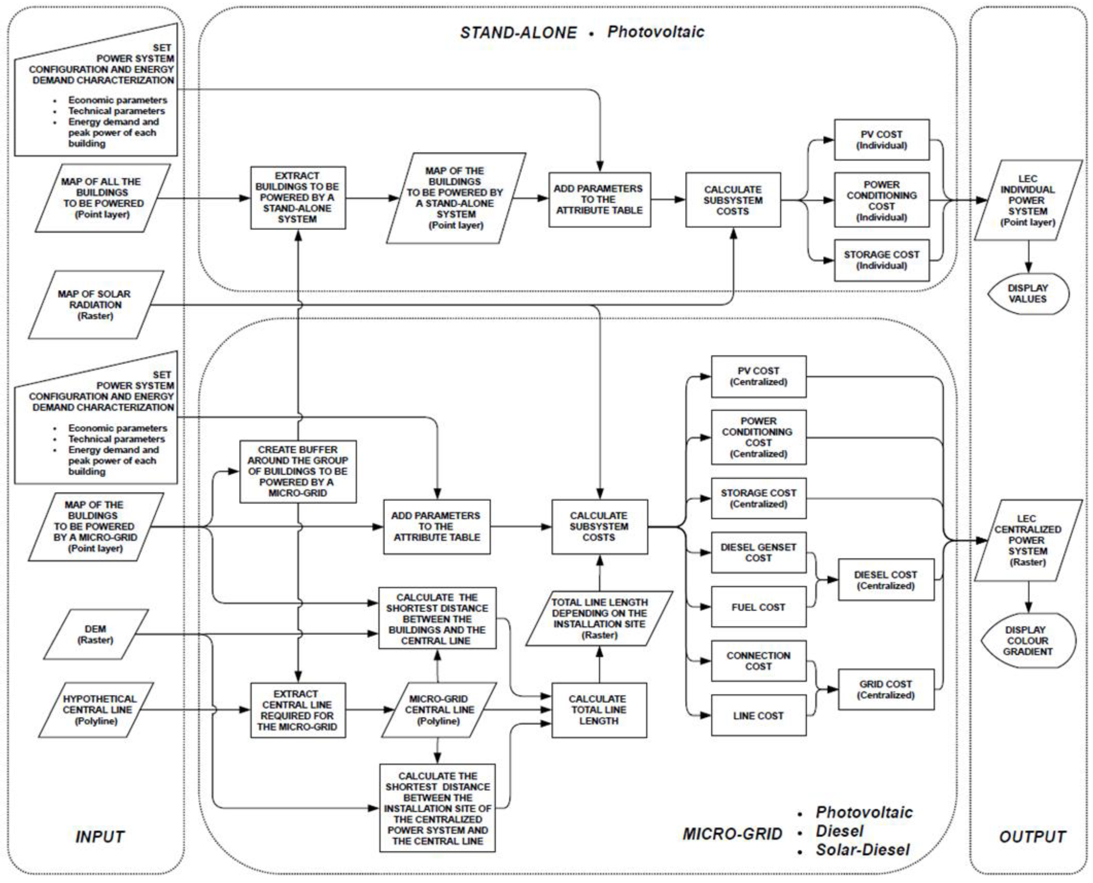
Figure 9.
(left) Point layer of the buildings in Guasasa (in green) and line layer of the central distribution line (dotted). (Right): Point layer of the group of buildings to be centralized (in red) and portion of distribution line needed by the microgrid (in black). Also in red, the area used to extract the portion of line from the total.
Figure 9.
(left) Point layer of the buildings in Guasasa (in green) and line layer of the central distribution line (dotted). (Right): Point layer of the group of buildings to be centralized (in red) and portion of distribution line needed by the microgrid (in black). Also in red, the area used to extract the portion of line from the total.
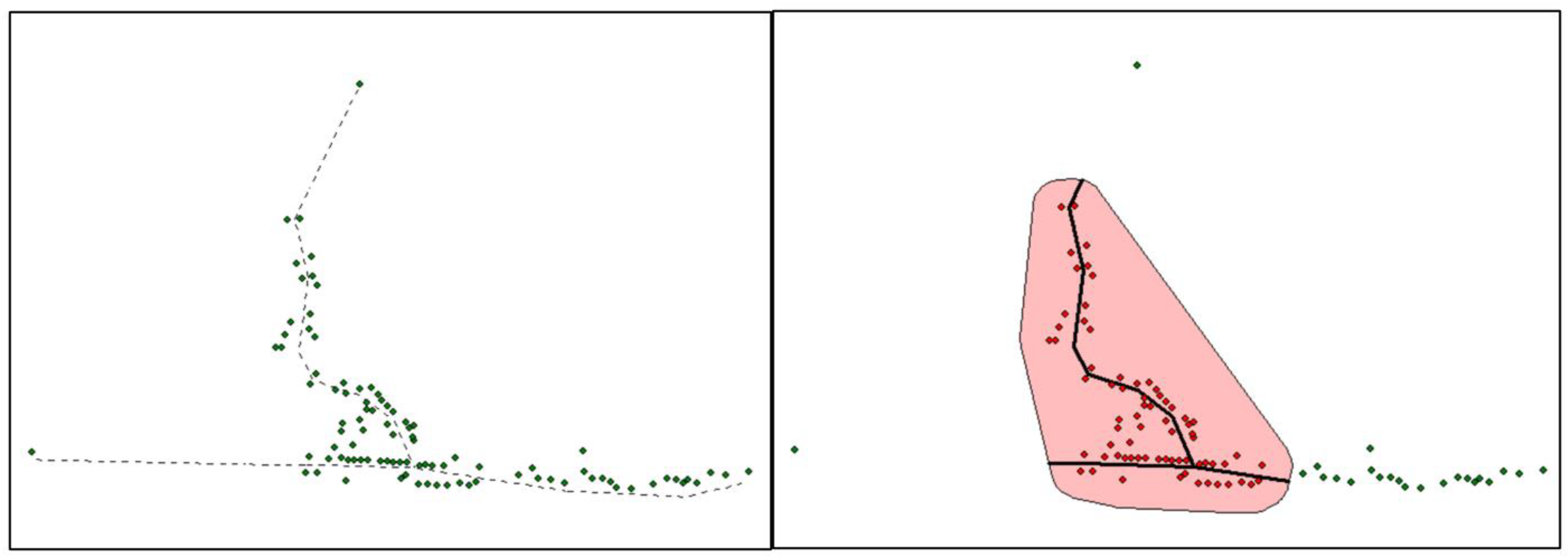
Figure 10.
DEM including the province of Matanzas. (Source: JAXA [84]).
Figure 10.
DEM including the province of Matanzas. (Source: JAXA [84]).
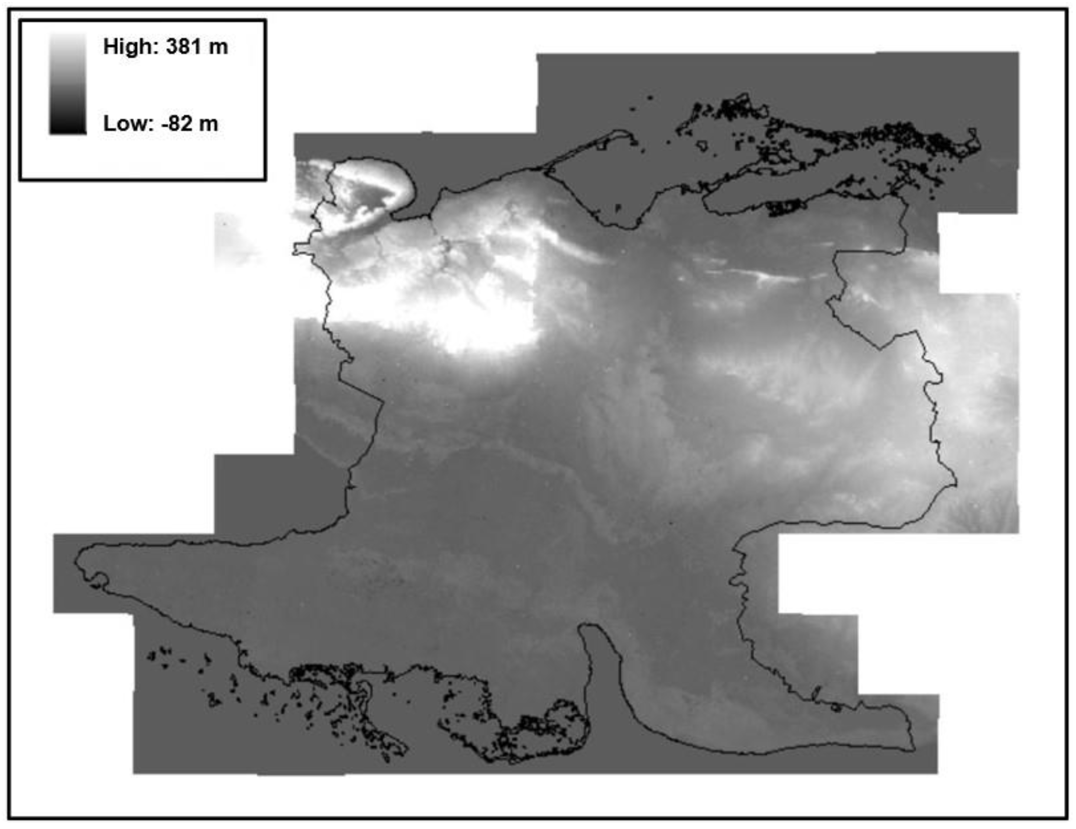
Figure 11.
Annual Global Solar Radiation on optimal angle tilted surface in Guasasa. .
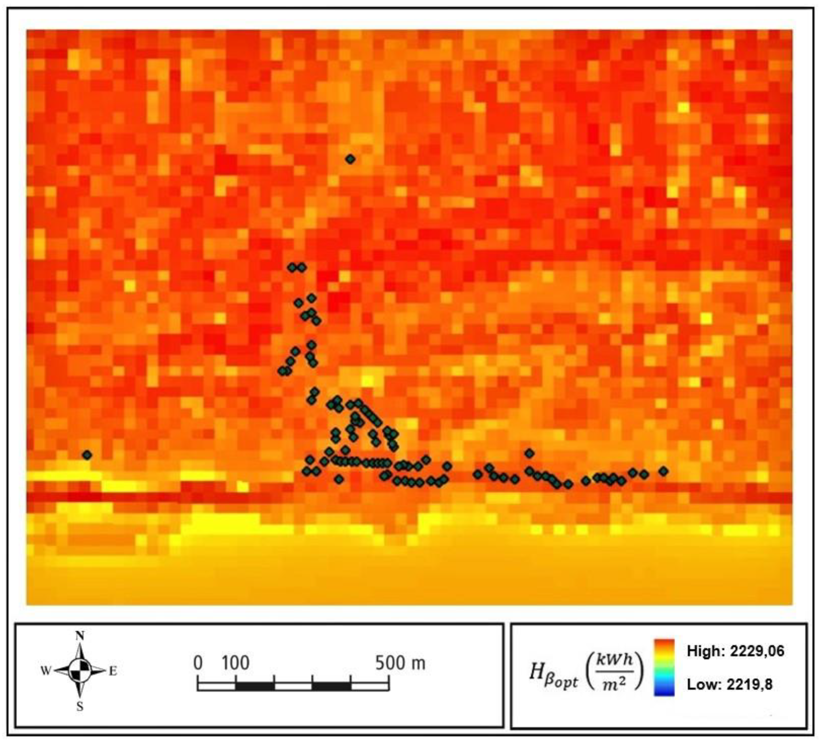
Figure 14.
Cost contribution of each subsystem to the total LEC of a PV centralized system for the three cases tested.
Figure 14.
Cost contribution of each subsystem to the total LEC of a PV centralized system for the three cases tested.
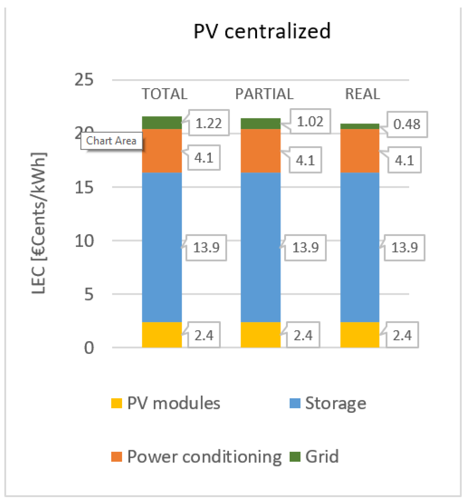
Figure 15.
Cost contribution of each subsystem to the total LEC of a diesel-PV (f.r.75%) system for the three cases tested.
Figure 15.
Cost contribution of each subsystem to the total LEC of a diesel-PV (f.r.75%) system for the three cases tested.
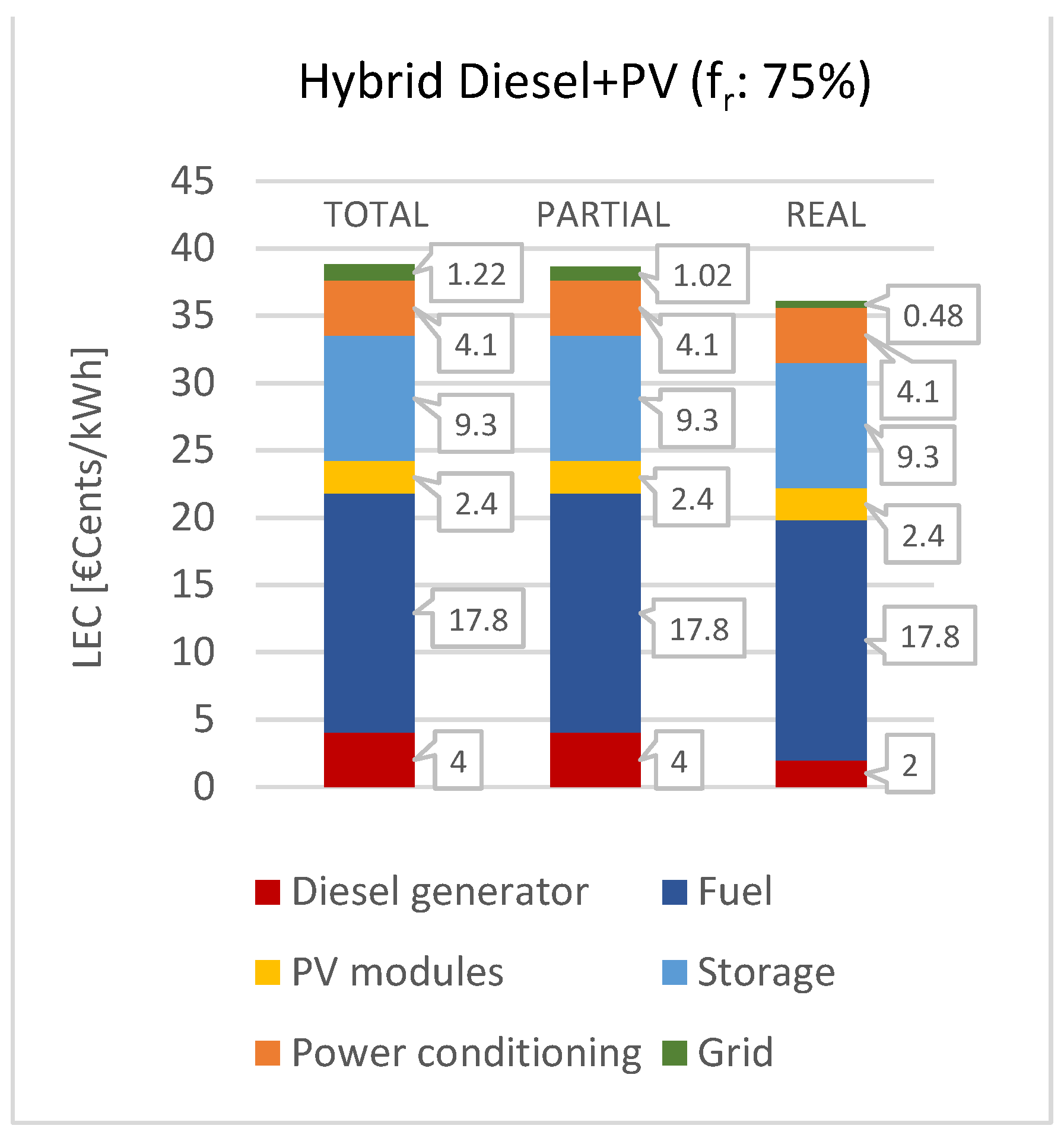
Figure 16.
Cost contribution of each subsystem to the total LEC of a diesel-PV (f.r.50%) system for the three cases tested.
Figure 16.
Cost contribution of each subsystem to the total LEC of a diesel-PV (f.r.50%) system for the three cases tested.
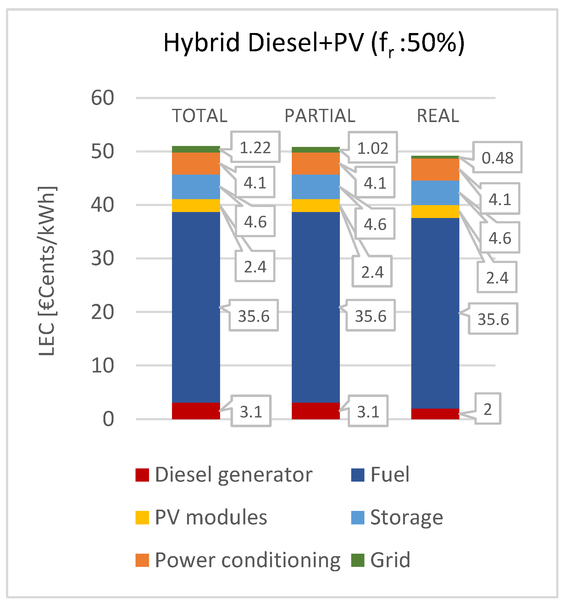
Figure 17.
Cost contribution of each subsystem to the total LEC of a diesel generator set for the three cases tested.
Figure 17.
Cost contribution of each subsystem to the total LEC of a diesel generator set for the three cases tested.
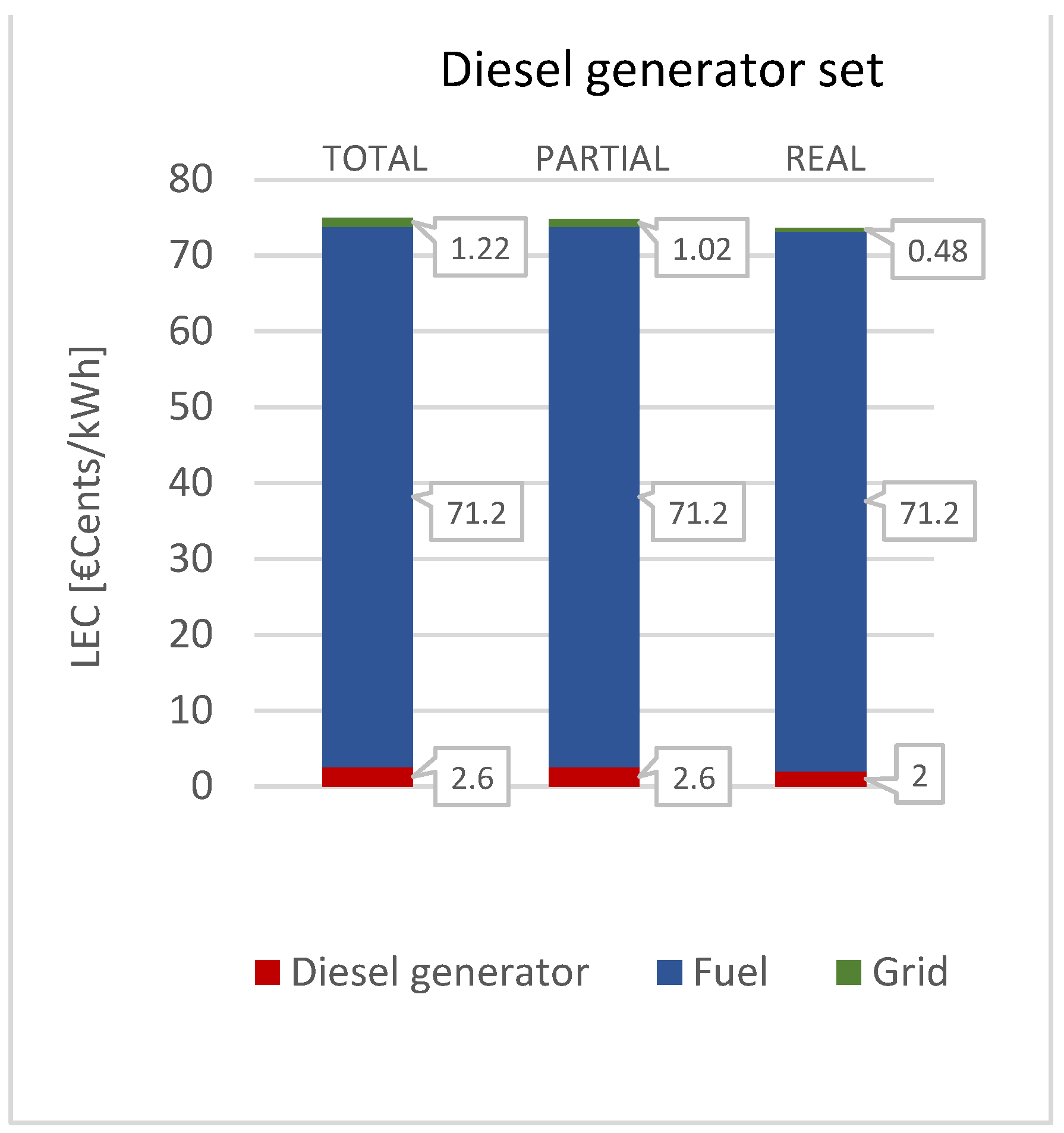
Figure 18.
LEC of a diesel-PV (f.r.75%) system in Guasasa with total centralization.

Figure 19.
LEC of a diesel-PV (f.r.75%) system in Guasasa with partial centralization.
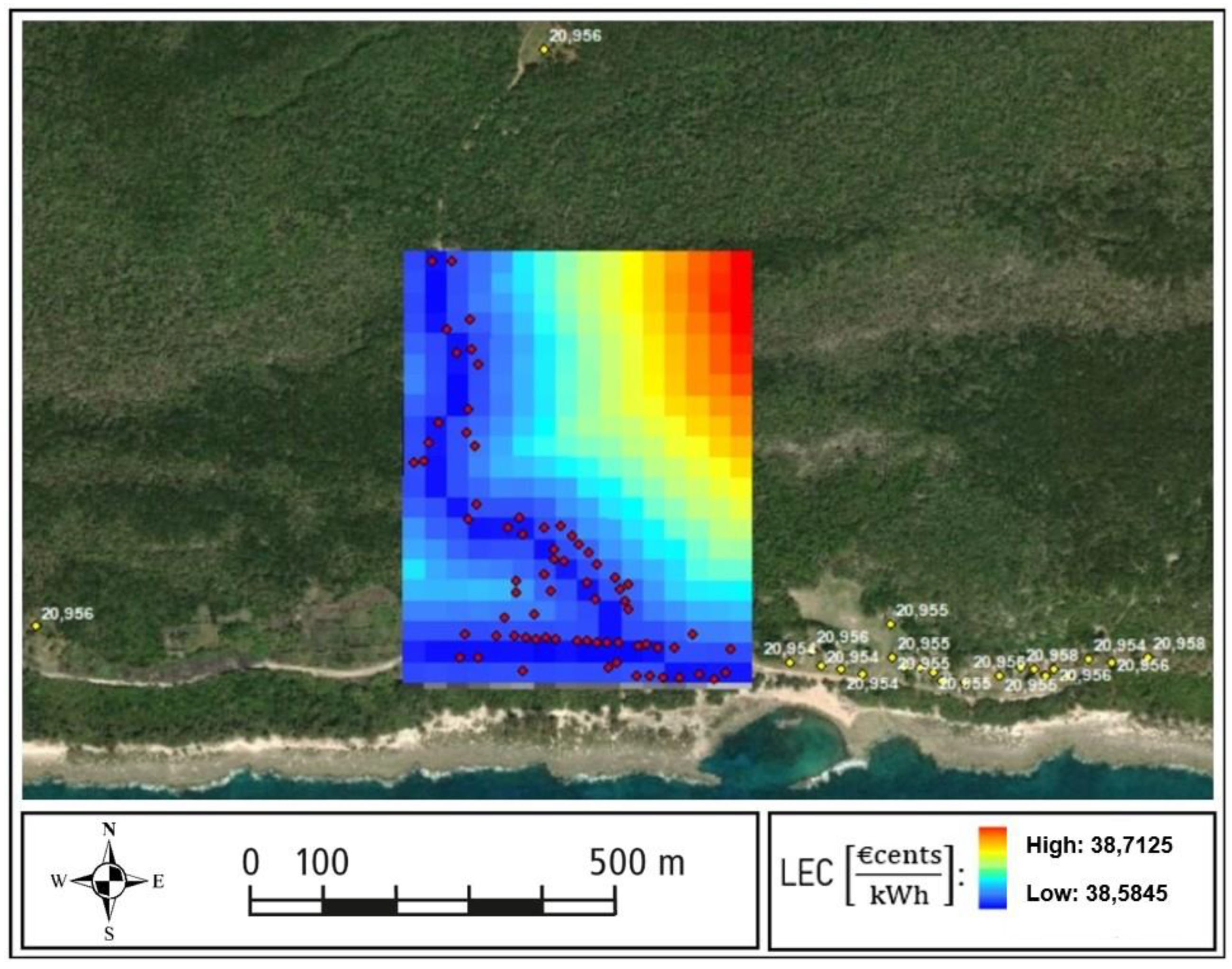
Figure 20.
LEC of a diesel-PV (f.r.75%) system in Guasasa for the real case.
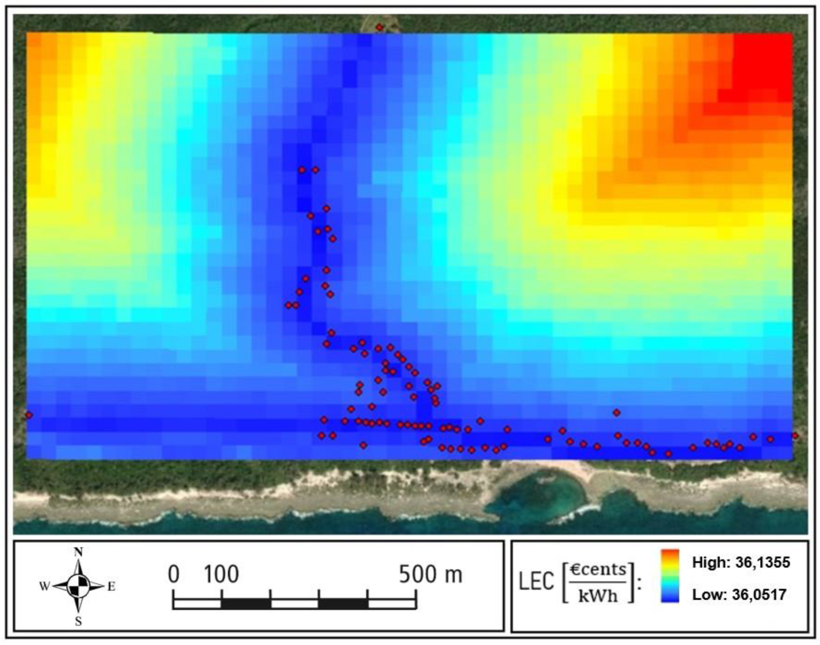
Figure 21.
LEC comparison of different types of power plant and contribution of each subsystem cost considering the ideal case and total centralization.
Figure 21.
LEC comparison of different types of power plant and contribution of each subsystem cost considering the ideal case and total centralization.
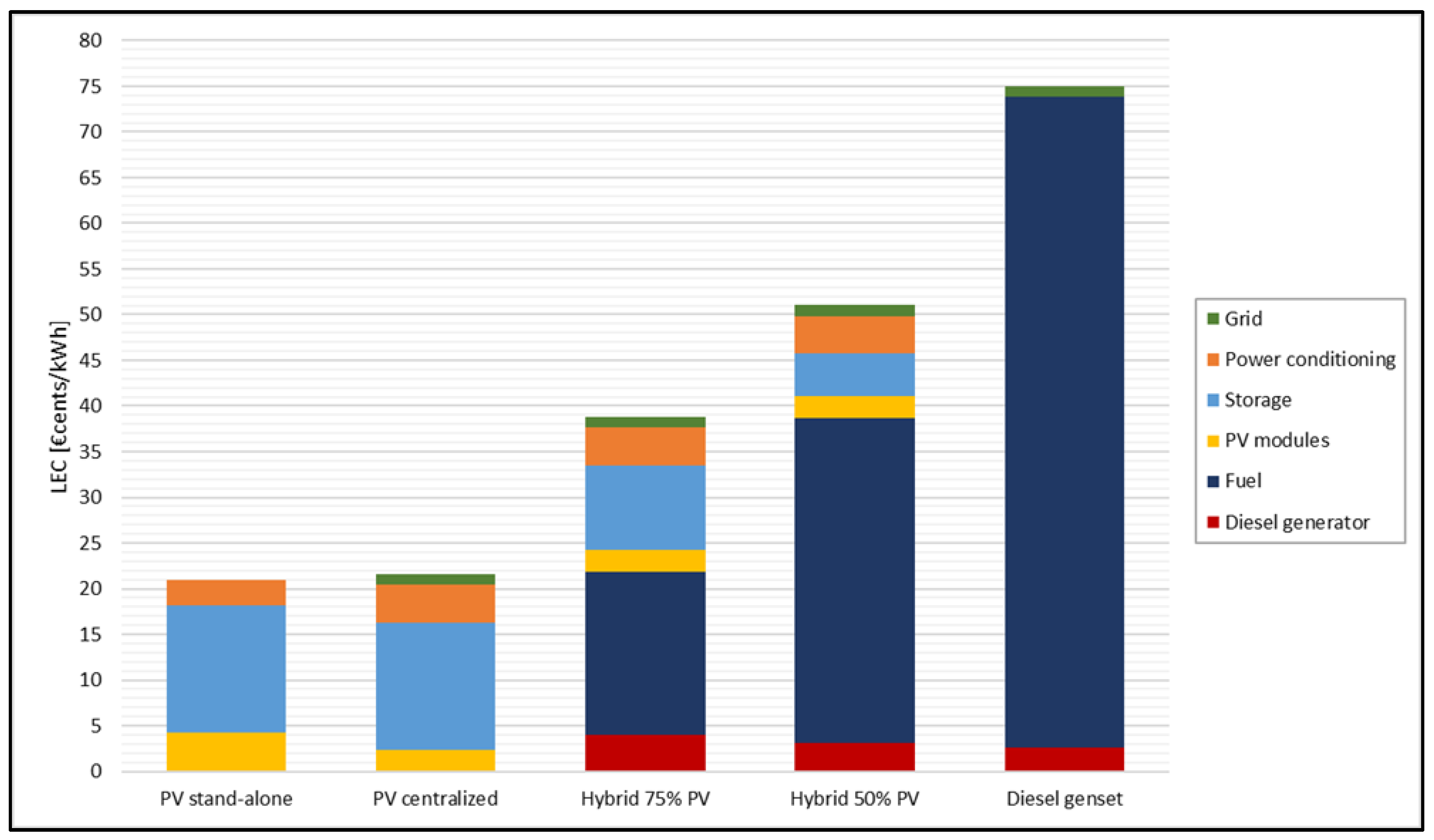
Figure 22.
LEC comparison of different types of power plant and contribution of each subsystem cost considering the ideal case and partial centralization.
Figure 22.
LEC comparison of different types of power plant and contribution of each subsystem cost considering the ideal case and partial centralization.
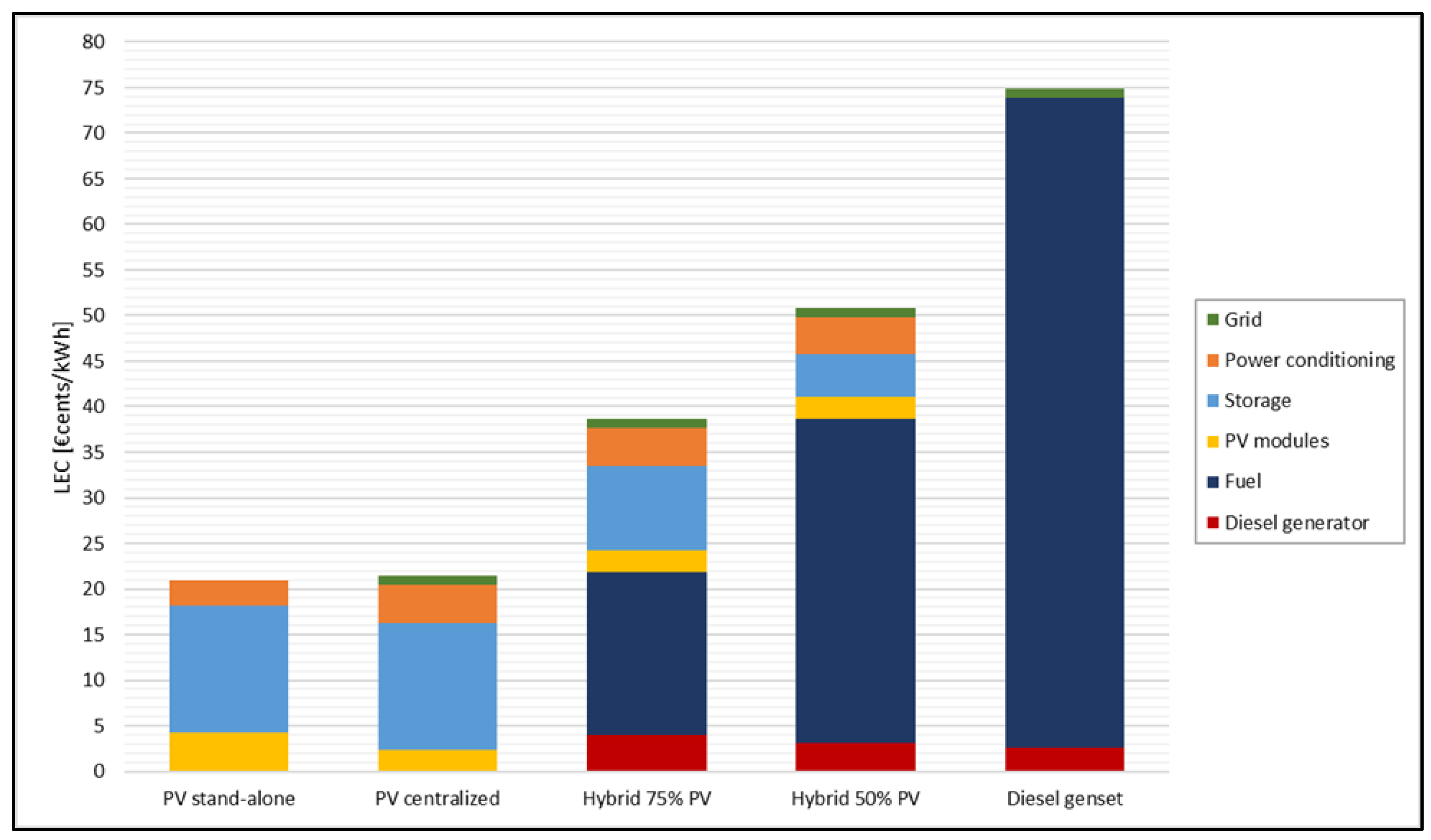
Figure 23.
LEC comparison of different types of power plant and contribution of each subsystem cost considering the real case.
Figure 23.
LEC comparison of different types of power plant and contribution of each subsystem cost considering the real case.
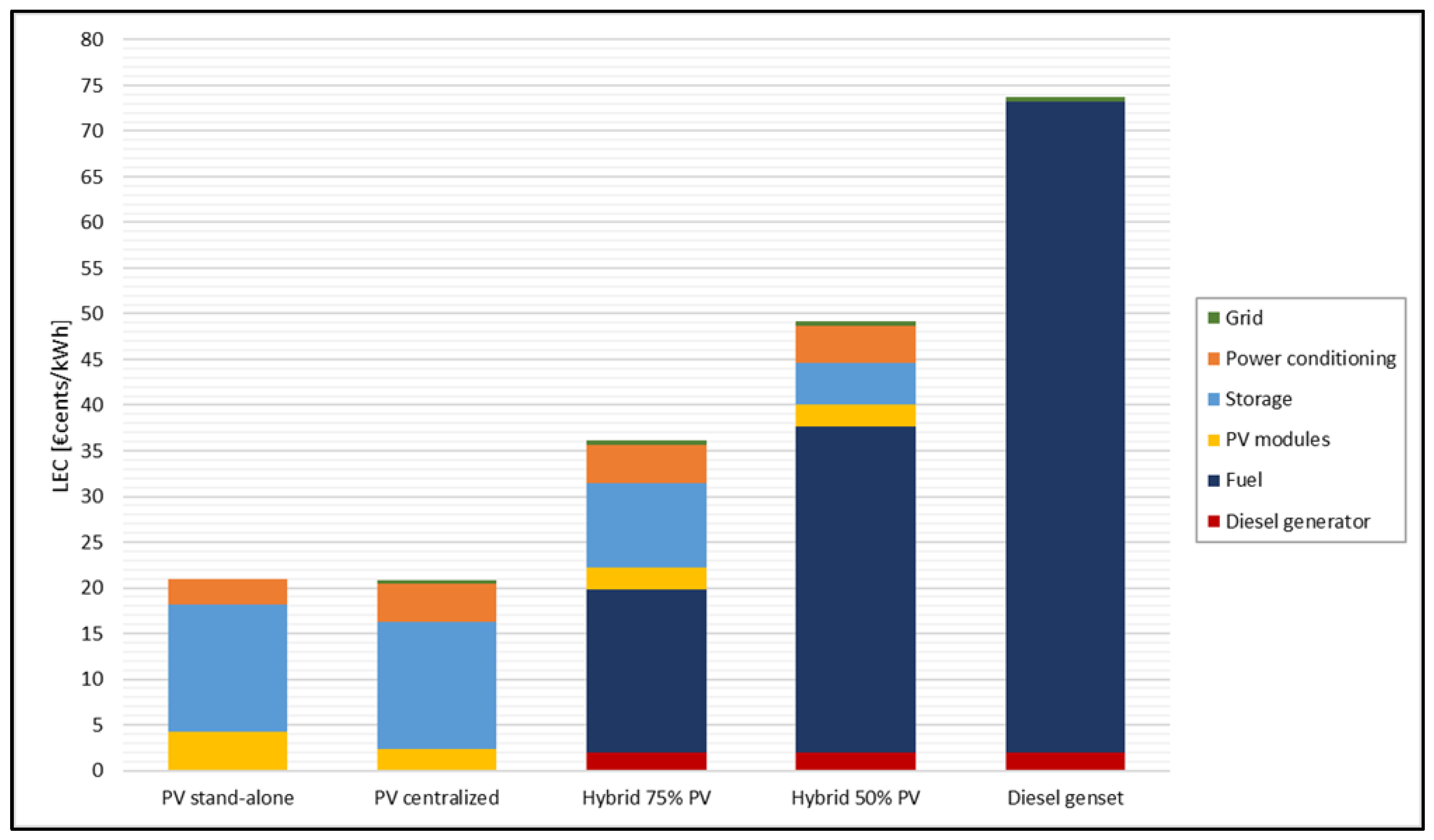
Table 2.
License plate of the diesel generator set currently operating in Guasasa.
| Engine-drive AC Generator DENYO | |
|---|---|
| Model | DCA-100 ESI |
| Brushless AC Generator | |
| Model | DB-1101L |
| Phases | 3 |
| Wires | 4 |
| Rated Output | 100 kVA |
| Rated Voltage | 220 V |
| Rated Current | 262 A |
| Frequency | 60 Hz |
| Rating | Continuous |
| Power Factor | 0.8 |
| Poles | 4 |
| Engine | |
| Model | DB-6BG1T |
| Rated Output | 91.3 kW – 1800 rpm |
| Piston displacement | 6494 l |
| Fuel | Diesel |
Table 4.
Results of the energy demand analysis of the Guasasa community [79].
Table 4.
Results of the energy demand analysis of the Guasasa community [79].
| Demand characterization | |
|---|---|
| Actual Energy Demand (12 h) | 265 kWh |
| Total Estimated Energy Demand | 437 kWh |
| Minimum Power | 12 kW |
| Peak Power | 34 kW |
Table 9.
Input settings for the energy storage and several renewable fraction.
| Type | ns | Is [€/kWh] | OMs[€/kWh] | d [days] | DoD | ||
|---|---|---|---|---|---|---|---|
| Storage | 18 | 180 | 4 | 85% | 3 | 70% | |
| Hybrid 75% | 18 | 180 | 4 | 85% | 2 | 70% | |
| Hybrid 50% | 18 | 180 | 4 | 85% | 1 | 70% |
Table 12.
Results of the calculation for a PV stand-alone system referred to a single house.
| CPV [€cents/kWh] | 4.3 |
| CS [€cents/kWh] | 13.9 |
| Cpc [€cents/kWh] | 2.8 |
| EPV [kWh/year] | 1642.5 |
| PPV [kW] | 1.1 |
| CFpv | 16.5% |
| LECpv [€cents/kWh] | 21 |
Table 13.
Results of the LEC model execution for a PV centralized system for the three cases tested.
Table 13.
Results of the LEC model execution for a PV centralized system for the three cases tested.
| Total | Partial | Real | |
|---|---|---|---|
| CPV [€cents/kWh] | 2.4 | 2.4 | 2.4 |
| CS [€cents/kWh] | 13.9 | 13.9 | 13.9 |
| Cpc [€cents/kWh] | 4.1 | 4.1 | 4.1 |
| CLV [€cents/kWh] | 1.07 | 0.87 | 0.48 |
| CCN [€cents/kWh] | 0.15 | 0.15 | - |
| EPV [MWh/year] | 160.93 | 115.85 | 160.93 |
| PPV [kW] | 90.4 | 65.1 | 90.4 |
| CFpv | 20.3% | 20.3% | 20.3% |
| LECcentr [€cents/kWh] | 21.6 | 21.4 | 20.9 |
Table 14.
Results of the LEC model execution for a diesel-PV (r.f.75%) system for the three cases tested.
Table 14.
Results of the LEC model execution for a diesel-PV (r.f.75%) system for the three cases tested.
| Total | Partial | Real | |
|---|---|---|---|
| CD [€cents/kWh] | 4 | 4 | 2 |
| CF [€cents/kWh] | 17.8 | 17.8 | 17.8 |
| CPV [€cents/kWh] | 2.4 | 2.4 | 2.4 |
| CS [€cents/kWh] | 9.3 | 9.3 | 9.3 |
| Cpc [€cents/kWh] | 4.1 | 4.1 | 4.1 |
| CLV [€cents/kWh] | 1.07 | 0.87 | 0.48 |
| CCN [€cents/kWh] | 0.15 | 0.15 | - |
| EDiesel [MWh/year] | 40.23 | 28.96 | 40.23 |
| PDiesel [kW] | 66.6 | 48.7 | 80 |
| CFDiesel | 6.90% | 6.80% | 5.70% |
| EPV [MWh/year] | 120.70 | 86.89 | 120.70 |
| PPV [kW] | 67.8 | 48.8 | 67.8 |
| CFpv | 20.30% | 20.30% | 20.30% |
| LECcentr [€cents/kWh] | 38.8 | 38.6 | 36.1 |
Table 15.
Results of the LEC model execution for a diesel-PV (r.f.50%) system for the three cases tested.
Table 15.
Results of the LEC model execution for a diesel-PV (r.f.50%) system for the three cases tested.
| Total | Partial | Real | |
|---|---|---|---|
| CD [€cents/kWh] | 3.1 | 3.1 | 2 |
| CF [€cents/kWh] | 35.6 | 35.6 | 35.6 |
| CPV [€cents/kWh] | 2.4 | 2.4 | 2.4 |
| CS [€cents/kWh] | 4.6 | 4.6 | 4.6 |
| Cpc [€cents/kWh] | 4.1 | 4.1 | 4.1 |
| CLV [€cents/kWh] | 1.07 | 0.87 | 0.48 |
| CCN [€cents/kWh] | 0.15 | 0.15 | - |
| EDiesel [MWh/year] | 80.46 | 57.93 | 80.46 |
| PDiesel [kW] | 66.6 | 48.7 | 80 |
| CFDiesel | 13.80% | 13.60% | 11.50% |
| EPV [MWh/year] | 80.46 | 57.93 | 80.46 |
| PPV [kW] | 45.2 | 32.53 | 45.2 |
| CFpv | 20.30% | 20.30% | 20.30% |
| LECcentr [€cents/kWh] | 51.0 | 50.8 | 49.2 |
Table 16.
Results of the LEC model execution for a diesel generator set for the three cases tested.
| Total | Partial | Real | |
|---|---|---|---|
| CD [€cents/kWh] | 2.6 | 2.6 | 2 |
| CF [€cents/kWh] | 71.2 | 71.2 | 71.2 |
| CLV [€cents/kWh] | 1.07 | 0.87 | 0.48 |
| CCN [€cents/kWh] | 0.15 | 0.15 | - |
| EDiesel [MWh/year] | 160.93 | 115.85 | 160.93 |
| PDiesel [kW] | 66.6 | 48.7 | 80 |
| CFDiesel | 27.6% | 27.1% | 23% |
| LECcentr [€cents/kWh] | 75.0 | 74.8 | 73.7 |
Table 17.
LEC (€cents/kWh) of different types of power plant and contribution of each subsystem cost considering the ideal case and total centralization.
Table 17.
LEC (€cents/kWh) of different types of power plant and contribution of each subsystem cost considering the ideal case and total centralization.
| TOTAL | Diesel | PV | Storage | PC | Fuel | Line | Total |
|---|---|---|---|---|---|---|---|
| PV stand-alone | 0 | 4.3 | 13.9 | 2.8 | 0 | 0 | 21.0 |
| PV centralized | 0 | 2.4 | 13.9 | 4.1 | 0 | 1.2 | 21.6 |
| Hybrid 75% PV | 4.0 | 2.4 | 9.3 | 4.1 | 17.8 | 1.2 | 38.8 |
| Hybrid 50% PV | 3.1 | 2.4 | 4.6 | 4.1 | 35.6 | 1.2 | 51.0 |
| Diesel genset | 2.6 | 0 | 0 | 0 | 71.2 | 1.2 | 75.0 |
Table 18.
LEC (€cents/kWh) of different types of power plant and contribution of each subsystem cost considering the ideal case and partial centralization.
Table 18.
LEC (€cents/kWh) of different types of power plant and contribution of each subsystem cost considering the ideal case and partial centralization.
| PARTIAL | Diesel | PV | Storage | PC | Fuel | Line | Total |
|---|---|---|---|---|---|---|---|
| PV stand-alone | 0 | 4.3 | 13.9 | 2.8 | 0 | 0 | 21.0 |
| PV centralized | 0 | 2.4 | 13.9 | 4.1 | 0 | 1.0 | 21.4 |
| Hybrid 75% PV | 4.0 | 2.4 | 9.3 | 4.1 | 17.8 | 1.0 | 38.6 |
| Hybrid 50% PV | 3.1 | 2.4 | 4.6 | 4.1 | 35.6 | 1.0 | 50.8 |
| Diesel genset | 2.6 | 0 | 0 | 0 | 71.2 | 1.0 | 74.8 |
Table 19.
LEC (€cents/kWh) of different types of power plant and contribution of each subsystem cost considering the real case.
Table 19.
LEC (€cents/kWh) of different types of power plant and contribution of each subsystem cost considering the real case.
| REAL | Diesel | PV | Storage | PC | Fuel | Line | Total |
|---|---|---|---|---|---|---|---|
| PV stand-alone | 0 | 4.3 | 13.9 | 2.8 | 0 | 0 | 21.0 |
| PV centralized | 0 | 2.4 | 13.9 | 4.1 | 0 | 0.5 | 20.9 |
| Hybrid 75% PV | 2.0 | 2.4 | 9.3 | 4.1 | 17.8 | 0.5 | 36.1 |
| Hybrid 50% PV | 2.0 | 2.4 | 4.6 | 4.1 | 35.6 | 0.5 | 49.2 |
| Diesel genset | 2.0 | 0 | 0 | 0 | 71.2 | 0.5 | 73.7 |
Disclaimer/Publisher’s Note: The statements, opinions and data contained in all publications are solely those of the individual author(s) and contributor(s) and not of MDPI and/or the editor(s). MDPI and/or the editor(s) disclaim responsibility for any injury to people or property resulting from any ideas, methods, instructions or products referred to in the content. |
© 2024 by the authors. Licensee MDPI, Basel, Switzerland. This article is an open access article distributed under the terms and conditions of the Creative Commons Attribution (CC BY) license (http://creativecommons.org/licenses/by/4.0/).
Copyright: This open access article is published under a Creative Commons CC BY 4.0 license, which permit the free download, distribution, and reuse, provided that the author and preprint are cited in any reuse.


