Solving the Hubble Tension Using the PantheonPlusSH0ES Supernova Database

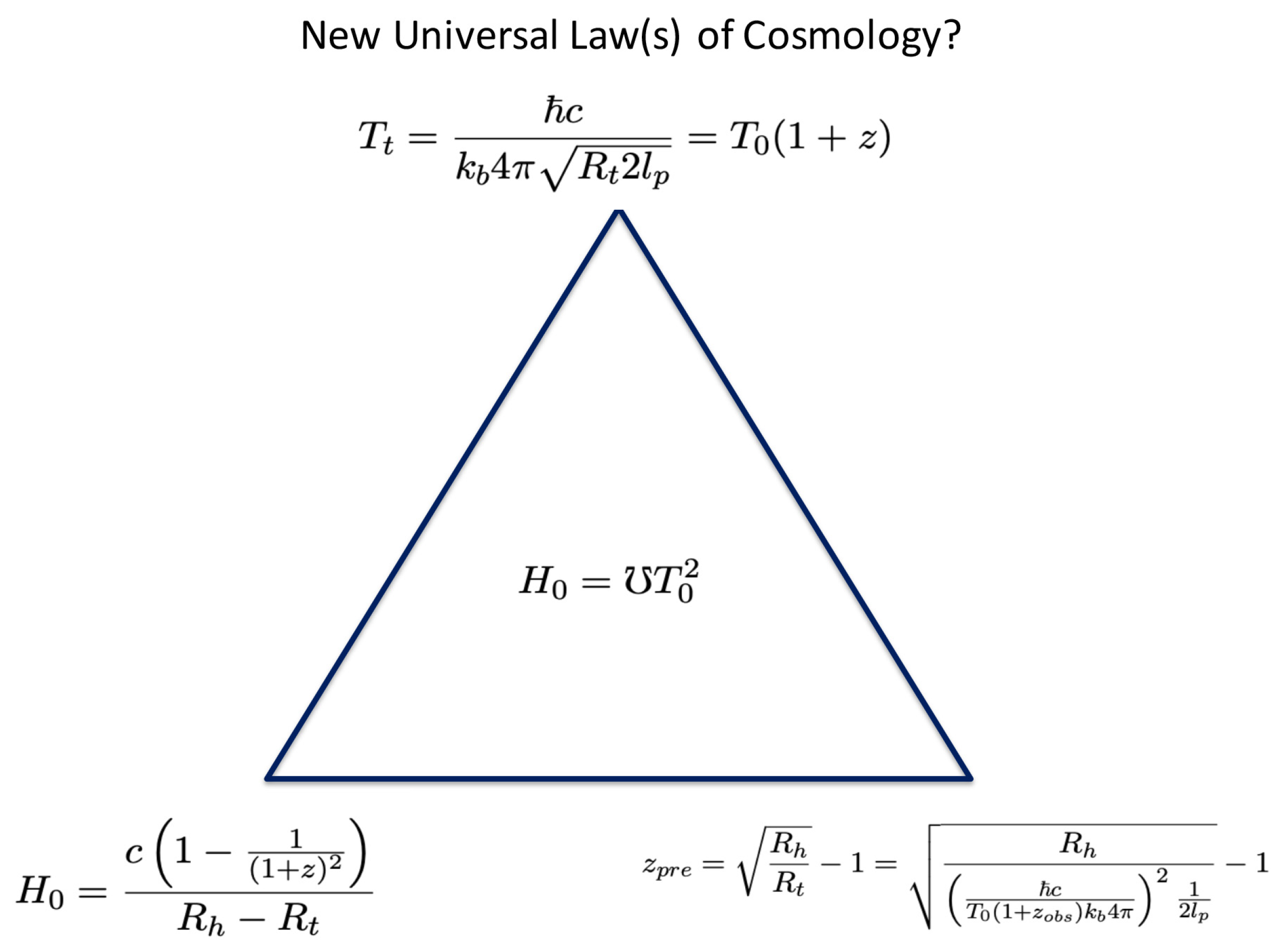
1. The CMB Temperature Prediction Formula

Tatum et al [1] presented the following formula for the Cosmic Microwave Background (CMB) temperature in 2015, a formula which has been discussed in more depth and derived from the Stefan-Boltzmann law [2,3] recently by Haug and Wojnow [4,5]:

$$T_{CMB,0}={\displaystyle \frac{\hslash c^3}{k_{b}8\pi G\sqrt{M_c{m}_p}}}={\displaystyle \frac{\hslash c}{k_{b}4\pi \sqrt{R_{H}2l_p}}}$$

(1)

where $k_b$ is the Boltzmann constant, $R_H={\displaystyle \frac{c}{H_t}}$ is the Hubble radius, G is the Newtonian gravitational constant, $l_p=\sqrt{{\displaystyle \frac{G\hslash }{c^3}}}$ is the Planck length, $m_p=\sqrt{{\displaystyle \frac{\hslash c}{G}}}$ is the Planck mass, c is the speed of light, and $\hslash ={\displaystyle \frac{h}{2\pi }}$ is the reduced Planck constant, also known as the Dirac constant. $M_H$ is the current equivalent mass in the Hubble sphere, where we can use the critical Friedmann mass $M_c={\displaystyle \frac{c^2{R}_H}{2G}}$ as the mass now. This implies that the Schwarzschild radius in the critical Friedmann universe is identical to the Hubble radius, something that is well known (see [6,7]); possible connections between the Hubble sphere and black holes have been discussed since at least 1972 (see [8]) and are actively discussed to this day (see [9,10,11,12]). Despite its likely great potential significance, this formula (Eq. 1) has received little attention from the wider astrophysics community.

The Stefan-Boltzmann law is valid for nearly perfect black bodies. Based on extensive studies made by the COBE satellite, Muller et al. [13] state (see also [14]):

“Observations with the COBE satellite have demonstrated that the CMB corresponds to a nearly perfect black body characterized by a temperature $T_0$ at $z=0$, which is measured with very high accuracy, $T_0=2.72548\pm 0.00057 K$."

Therefore, it should not be a surprise that the Stefan-Boltzmann law can be used to derive the CMB temperature. One may question whether this law was also valid during earlier epochs of the universe. With the $\Lambda$CDM model, this is unlikely; however, our CMB formula is consistent with $R_h=ct$ cosmology, which we will discuss shortly.

It is worth noting that Equation (1) looks quite similar to the Hawking black hole temperature formula [15,16]: $T_{Hw}={\displaystyle \frac{\hslash c^3}{k_{b}8\pi GM}}$, except that one replaces M with $\sqrt{M_c{m}_p}$.

Based on Equation (1), we can calculate the current CMB temperature using the current Hubble constant value of $H_0=67.4\pm 0.5\mathrm{km}/\mathrm{s}/\mathrm{Mpc}$ as given by the Particle Data Group (PDG)1 in their Astrophysical Constants and Parameters. From Equation (1), we obtain $T_0={2.7358}_{-0.0101}^{+0.0102}\mathrm{K}$. This result shows that the constraint on the CMB temperature given by the PDG ($T_0={2.7255}_{-0.0006}^{+0.0006}\mathrm{K}$) is within our predicted range, indicating that our model is not in conflict with these established measurements.

Our uncertainty in $T_0$ is indeed larger than that given by the observational study cited by the PDG. The reason for this is that our CMB temperature is a predicted value based on a new mathematical relation between $H_0$ and $T_0$ (Equation (1)). When predicting $T_0$ from $H_0$, the uncertainty in $T_0$ is inherently linked to the uncertainty in the observed $H_0$. The $\Lambda$-CDM model, however, does not predict $T_0$, making our approach noteworthy.

There is a duality in our formula: a CMB temperature of $T_0=2.7255$ K corresponds to $H_0\approx 66.9\mathrm{km}/\mathrm{s}/\mathrm{Mpc}$, and vice versa (we will soon come back to the confidence intervals based on measurement inputs and how they affect our model). In other words, both the current CMB temperature and $H_0$ in this duality fall well within the constraints set for these cosmological parameters by the Particle Data Group (PDG). The beauty of this new exact mathematical relation between CMB temperature and $H_0$ is that we can now rely on the most precisely-measured of the two to predict the other one with high precision, something which will become more clear as one goes through this manuscript, as well as the papers referred to.

Although Equation (1) has recently been demonstrated to be derivable from the Stefan-Boltzmann law [4,5], Haug and Tatum [17] have also derived the same formula from a geometric mathematical approach, demonstrating its consistency with a geometric mean temperature between the lowest and highest possible current temperatures in the Hubble sphere. We are not the first to use geometric means in thermodynamics; see also Henderson [18]. Even a third alternative and compatible way to derive Equation (1) exists, based on the fact that the minimum light bending is linked to the Planck scale; see [19]. These radically different approaches, in addition to the Stefan-Boltzmann derivation, suggest that Equation (1) has a solid physical foundation.

All of these approaches seem to create a consistent and interesting framework, particularly in line with “growing black hole” models such as the FSC Schwarzschild metric model, but likely also other growing black hole models that can be built around other metrics, such as [20,21,22,23].

An actively discussed class of cosmological models, for comparison to the $\Lambda$-CDM model, is the so-called $R_h=ct$ models (see, for example, [7,24,25,26,27,28]). Naturally, there are also critics of the $R_h=ct$ models, and such discussions are essential for progress in research. Lewis [29], for example, has criticized the $R_h=ct$ model for its “unphysical properties;” however, these claims have been refuted by Melia [30]. Melia [31] also published a study summarizing 18 observational tests comparing the $R_h=ct$ model with the $\Lambda$-CDM model and showing that most of these tests actually favor $R_h=ct$. Despite this, there are ongoing criticisms of the $R_h=ct$ model to this day, as seen in the recent paper by Panchal and Desai [32].

The FSC model, originating with the referenced Tatum et al (2015) paper, falls within the category of growing black hole variants of $R_h=ct$ models, which represent a subclass of $R_h=ct$ models. Thus, there is also thermodynamics related to the current and past CMB temperature in this cosmological model. A generalized version of formula (1) can be:

$$T_t=T_{CMB}\left(t\right)={\displaystyle \frac{\hslash c}{k_{b}4\pi \sqrt{R_{t}2l_p}}}$$

(2)

where $R_t$ is the black hole radius at any stage in the growing black hole universe. In this model, the universe starts out with a Planck mass Schwarzschild radius of $R_s={\displaystyle \frac{2G{m}_p}{c^2}}=2l_p$ and then expands one Planck length in radius per Planck time. Thus, one can also say that it increases by one-half a Planck mass per Planck time.

2. Cosmological Redshift from CMB Temperatures

In general, for many cosmological models, we have:

$$z={\displaystyle \frac{R\left(t_0\right)}{R\left(t\right)}}-1$$

(3)

where $R\left(t\right)$ is the scale factor dependent on the cosmological model, and $t_0$ is the reference time, which is now. In the $\Lambda$-CDM model, light is redshifted based on the idea of the expansion of space and cosmic time. The redshifted wavelength can be treated as stretching as space-time expands. In the FSC Tatum et al model, we have $R_0=R\left(t_0\right)={\displaystyle \frac{c}{H_0}}=R_H$, which is simply the Hubble radius $R_H={\displaystyle \frac{c}{H_0}}$ at present. The Hubble radius is the distance light has traveled since the beginning of the black hole universe, which in the FSC model started as a Planck mass black hole and today is the Hubble sphere with mass equal to the mass in the critical Friedmann [33] universe $M_H=M_c={\displaystyle \frac{c^2{R}_H}{2G}}$.

Melia [34] has pointed out that the cosmological redshift in the Friedmann-LeMaitre-Robertson-Walker (FLRW) metrics with constant space–time curvature, which he emphasizes must be the case when $a\left(t\right)=ct$ in the $R_h=ct$ universe, yields:

$$z={\displaystyle \frac{a\left(t_0\right)}{a\left(t_e\right)}}-1={\displaystyle \frac{t_0}{t_e}}-1=e^X-1$$

(4)

Here, $t_e$ represents the emission time and $t_0$ represents the observation time. Since $t_0={\displaystyle \frac{R_h}{c}}$ and we also can have $t_e={\displaystyle \frac{R_t}{c}}$ in the $R_h=ct$ universe, this implies that we also can have: $z={\displaystyle \frac{a\left(t_0\right)}{a\left(t_e\right)}}-1={\displaystyle \frac{R_0}{R_t}}-1$. When we reconcile this with our equation for the CMB temperature $\left(\right)$, we obtain:

$$1+z={\displaystyle \frac{a\left(t_0\right)}{a_{(}{t}_t)}}={\displaystyle \frac{R_H}{R_t}}={\displaystyle \frac{{\left(\frac{\hslash c}{k_{b}4\pi \sqrt{R_{t}2l_p}}\right)}^2}{{\left(\frac{\hslash c}{k_{b}4\pi \sqrt{R_{H}2l_p}}\right)}^2}}={\displaystyle \frac{T_t^2}{T_0^2}}$$

(5)

where $R_H={\displaystyle \frac{c}{H_0}}$ and $R_t={\displaystyle \frac{c}{H_t}}$. Alternatively, we could write this as:

$$\begin{array}{ccc}\hfill z& =& {\displaystyle \frac{{\lambda }_{\mathrm{observed}}-{\lambda }_{\mathrm{emitted}}}{{\lambda }_{\mathrm{emitted}}}}={\displaystyle \frac{R_H-R_t}{R_t}}={\displaystyle \frac{R_H}{R_t}}-1\hfill \end{array}$$

(6)

$$\begin{array}{ccc}& =& {\displaystyle \frac{{\left(\frac{\hslash c}{k_{b}4\pi \sqrt{R_{t}2l_p}}\right)}^2}{{\left(\frac{\hslash c}{k_{b}4\pi \sqrt{R_{H}2l_p}}\right)}^2}}-1={\displaystyle \frac{T_t^2}{T_0^2}}-1.\hfill \end{array}$$

(7)

Solving for $T_t$ gives:

$$T_t=T_0{(1+z)}^{1-\beta }=T_0{(1+z)}^{{\displaystyle \frac{1}{2}}}.$$

(8)

In the current paper we provide some detail about its derivation and additional discussion. Tatum and Seshavatharam have acknowledged that the formula $T_t=T_0(1+z)$ is likely valid and have used it in a recent paper [35]. Observational studies strongly support $T_t=T_0(1+z)$ (see [36,37,38]). Therefore, a model consistent with $T_0{(1+z)}^{{\displaystyle \frac{1}{2}}}$ is likely incorrect. This strongly indicates that $R_h=ct$ models, which rely on $1+z={\displaystyle \frac{a\left(t_0\right)}{a\left(t_t\right)}}={\displaystyle \frac{R_H}{R_t}}$, are likely wrong or incomplete.

It is also worth looking at the $R_t$ distance as a function of z and $H_0$ in the following way:

$$\begin{array}{ccc}\hfill z& =& {\displaystyle \frac{R_H}{R_t}}-1\hfill \\ \hfill R_t& =& {\displaystyle \frac{c}{H_0(1+z)}}.\hfill \end{array}$$

(9)

So, the distance to the observed redshift is then:

$$\begin{array}{ccc}\hfill R_H-R_t& =& R_H-{\displaystyle \frac{c}{H_0(1+z)}}\hfill \\ \hfill R_H-R_t& =& {\displaystyle \frac{c}{H_0}}-{\displaystyle \frac{c}{H_0(1+z)}}\hfill \\ \hfill R_H-R_t& =& {\displaystyle \frac{c}{H_0}}\left(1-{\displaystyle \frac{1}{(1+z)}}\right)\hfill \end{array}$$

(10)

and solved for $H_0$ we have:

$$H_0={\displaystyle \frac{c}{d}}\left(1-{\displaystyle \frac{1}{(1+z)}}\right)$$

(11)

where $d=R_H-R_t$ is the estimated distance to the object emitting the photons.

When $z\ll 1$ we can use the first term of the Taylor series expansion which is:

$$\begin{array}{ccc}\hfill R_H-R_t& \approx & {\displaystyle \frac{cz}{H_0}}\hfill \end{array}$$

(12)

and naturally:

$$z\approx {\displaystyle \frac{d{H}_0}{c}}$$

(13)

where $d=R_H-R_t$ is the distance to the object emitting the photon, that is identical to the standard $\Lambda$-CDM cosmological redshift prediction formula typically used for low z values.

3. Comparison of ${\mathit{T}}_{\mathit{t}}={\mathit{T}}_{\mathit{0}}\sqrt{\mathbf{1}+\mathit{z}}$ versus ${\mathit{T}}_{\mathit{t}}={\mathit{T}}_{\mathbf{0}}(\mathbf{1}+\mathit{z})$

The $\Lambda$-CDM model has, for many years, been using the following relation between CMB temperature and redshift:

$$T_t=T_0(1+z).$$

(14)

As there has been some uncertainty as to whether this really is the best model of CMB temperature versus cosmological red shift z, Lima et al. [39] suggested the following generalization of the formula:

$$T_t=T_0{(1+z)}^{1-\beta }$$

(15)

where $\beta$ is an unknown constant that, if set to zero, yields the standard formula $T_t=T_0(1+z)$; however, it has also been suggested that $\beta$ can be other than zero. Chluba [40] has suggested that: “decay of vacuum energy leads to ‘adiabatic’ photon production (or destruction), such that the CMB temperature scales like$T_t=T_0{(1+z)}^{1-\beta }$."

Research based on observations has confirmed that $\beta$ should be close to zero; see again [36,37,38]. Thus, there is strong observational support for $T_t=T_0(1+z)$.

If we set $\beta =0$ then we can “only”2 make $T_t=T_0(1+z)$ compatible with CMB equations (1) and (2) in the following manner:

$$\begin{array}{ccc}\hfill z& =& {\displaystyle \frac{{\lambda }_{observed}-{\lambda }_{emitted}}{{\lambda }_{emitted}}}={\displaystyle \frac{\sqrt{R_H}-\sqrt{R_t}}{\sqrt{R_t}}}=\sqrt{{\displaystyle \frac{R_H}{R_t}}}-1\hfill \end{array}$$

(16)

$$\begin{array}{ccc}& =& {\displaystyle \frac{\left(\frac{\hslash c}{k_{b}4\pi \sqrt{R_{t}2l_p}}\right)}{\left(\frac{\hslash c}{k_{b}4\pi \sqrt{R_{H}2l_p}}\right)}}-1={\displaystyle \frac{T_t}{T_0}}-1.\hfill \end{array}$$

(17)

This means that we have $a\left(\sqrt{t}\right)=\sqrt{ct}$ and $R_h=ct$, that again gives: $z={\displaystyle \frac{a\left(\sqrt{t_0}\right)}{a\left(\sqrt{t_e}\right)}}-1=\sqrt{{\displaystyle \frac{R_H}{R_t}}}-1$, since $t_0={\displaystyle \frac{R_H}{c}}={\displaystyle \frac{1}{H_0}}$ and $t_e={\displaystyle \frac{R_t}{c}}={\displaystyle \frac{1}{H_t}}$. Even if the scale factor and cosmological redshift now are functions of $\sqrt{t}$ rather than t, the Hubble radius is still a linear function of t, namely still according to $R_h=ct$.

In this case, $T_t=T_0(1+z)$ will give the same prediction as in the previous sections where we instead had $T_t=T_0{(1+z)}^{{\displaystyle \frac{1}{2}}}$, something that only can be true if we now also have $z={\displaystyle \frac{\sqrt{R_H}}{\sqrt{R_t}}}-1$ rather than $z={\displaystyle \frac{R_H}{R_t}}-1$. This new possibility of setting: $z=\sqrt{{\displaystyle \frac{R_H}{R_t}}}-1$, should be carefully investigated, as this potentially could have an impact on how one interprets space expansion in accordance with $R_h=ct$ models and also how this can be considered in relation to the $\Lambda$-CDM model.

Riechers et al [38] have reported the Cosmic Microwave Background (CMB) temperature from the cosmic epoch at $z=6.34$, resulting in a temperature range of $16.4-30.2K$ within one standard deviation uncertainty. In other words, even the one standard deviation, which represents only about 68% probability for the CMB temperature to be inside that range, is very wide. The two standard deviation CMB temperature range is much broader. Therefore, we can conclude that the formula $T_t=T_0(1+z)$ is not sufficiently well-tested, given the very large uncertainty. The formula $T_t=T_0\sqrt{1+z}$ predicts a CMB temperature of $T_t=2.725K\sqrt{1+6.34}\approx 7.4K$ which is inside the 95% confidence interval of the above report (using two standard deviations); however, as we have also shown, the FSC framework at present also appears to be consistent with $T_t=T_0(1+z)$. Only further investigation can help us to decide on the optimal choice, even if observations appear to currently favor $\beta =0$.

It is also worth looking at the $R_t$ distance as a function of z and $H_0$ in the following way:

$$\begin{array}{ccc}\hfill z& =& \sqrt{{\displaystyle \frac{R_H}{R_t}}}-1\hfill \\ \hfill {(z+1)}^2& =& {\displaystyle \frac{R_H}{R_t}}\hfill \\ \hfill R_H& =& {(1+z)}^2{R}_t\hfill \\ \hfill R_t& =& {\displaystyle \frac{R_H}{{(1+z)}^2}}\hfill \\ \hfill R_t& =& {\displaystyle \frac{c}{H_0{(1+z)}^2}}.\hfill \end{array}$$

(18)

So, the distance to the observed redshift is then:

$$\begin{array}{ccc}\hfill R_H-R_t& =& R_H-{\displaystyle \frac{c}{H_0{(1+z)}^2}}\hfill \\ \hfill R_H-R_t& =& {\displaystyle \frac{c}{H_0}}-{\displaystyle \frac{c}{H_0{(1+z)}^2}}\hfill \\ \hfill R_H-R_t& =& {\displaystyle \frac{c}{H_0}}\left(1-{\displaystyle \frac{1}{{(1+z)}^2}}\right)\hfill \end{array}$$

(19)

and naturally:

$$H_0={\displaystyle \frac{c\left(1-\frac{1}{{(1+z)}^2}\right)}{D}}$$

(20)

where $D=R_H-R_t$, which is the distance between us and the object emitting the observed photons. When $z\ll 1$ we can use the first term of the first order Taylor series expansion and we get

$$D=R_H-R_t\approx {\displaystyle \frac{2cz}{H_0}}$$

(21)

that naturally gives:

$$z\approx {\displaystyle \frac{D{H}_0}{2c}}$$

(22)

and naturally:

$$H_0\approx {\displaystyle \frac{2zc}{D}}.$$

(23)

This is indeed different from the standard redshift formulation. However, in this case, the distance D will also differ from the distance predicted by the standard formula. Therefore, only careful further investigation can determine whether it is superior to the standard formula $z\approx {\displaystyle \frac{d{H}_0}{c}}$ or not. First of all, it is important to be aware that we have:

$$H_0\approx {\displaystyle \frac{2zc}{D}}={\displaystyle \frac{zc}{d}},z\approx {\displaystyle \frac{D{H}_0}{2c}}={\displaystyle \frac{d{H}_0}{c}}.$$

(24)

These two formulas give identical predictions for $H_0$ and z when dealing with short distances and low z. The ’2’ in the numerator is offset exactly by the fact that $D=2d$ in the denominator. This holds true when the distance is short ($z\ll 1$). Thus, when used to extract the Hubble constant from, for example, nearby supernovae, the estimated $H_0$ or estimated z are identical. It is the distances that differ in the two approaches. However, when dealing with supernovae or other objects far from us, the estimated Hubble constant values will be different, as we then need to use the exact formulas, rather than convenient approximations. This implies that, in the standard $\Lambda$-CDM model, the value of the Hubble constant based on higher redshifts is likely overestimated.

For redshift and Hubble constant analysis at short distances, we can say that the $\Lambda$-CDM model likely has two errors that cancel each other out: it has the wrong distance and also the wrong formula, which offsets the error in the wrong distance. Therefore, its predictions for redshift z and $H_0$ at short distances will be correct and the same as in our model. However, at much larger distances, their model will not be fully accurate, which we believe has led to the Hubble tension problem. This issue is addressed with our new way of looking at redshifts, as will become clear from the remainder of our paper, particularly in the sections where we aim to resolve the Hubble tension, namely Section 4 and Section 5.

If this latter redshift formula is correct, then distances to astronomical objects based on redshift are likely off by as much as a factor of 2. This could explain why the $\Lambda$-CDM model must have an expansion of space faster than $R_h=ct$ models. Once again, we believe that our new approach and explanation likely resolves the Hubble tension problem.

If one is not deeply entrenched in the topic, it may be easy to assume that our redshift equation (21) must be incorrect, given the highly precise measurements of distances to various astronomical objects through independent methods, such as parallax. However, supernova distances are never measured directly by a method as elementary as parallax. Establishing their distances requires a complex understanding of the astronomical distance ladder and the inherent uncertainties built into each rung of this ladder. Type Ia supernovae represent some of our most reliable standardized candles. Therefore, the most accurate method of determining their distance is likely through cosmological redshift, albeit this approach is naturally model-dependent. While our math, which suggests that the distance to the more remote supernovae is significantly greater than that predicted by the $\Lambda$-CDM model, may initially seem unfeasible, based on our current limited knowledge, it should not be immediately discounted. The above text following equation (23) we believe to be the crux of this paper. We would welcome any compelling arguments against our findings, in particular after studying the rest of our paper.

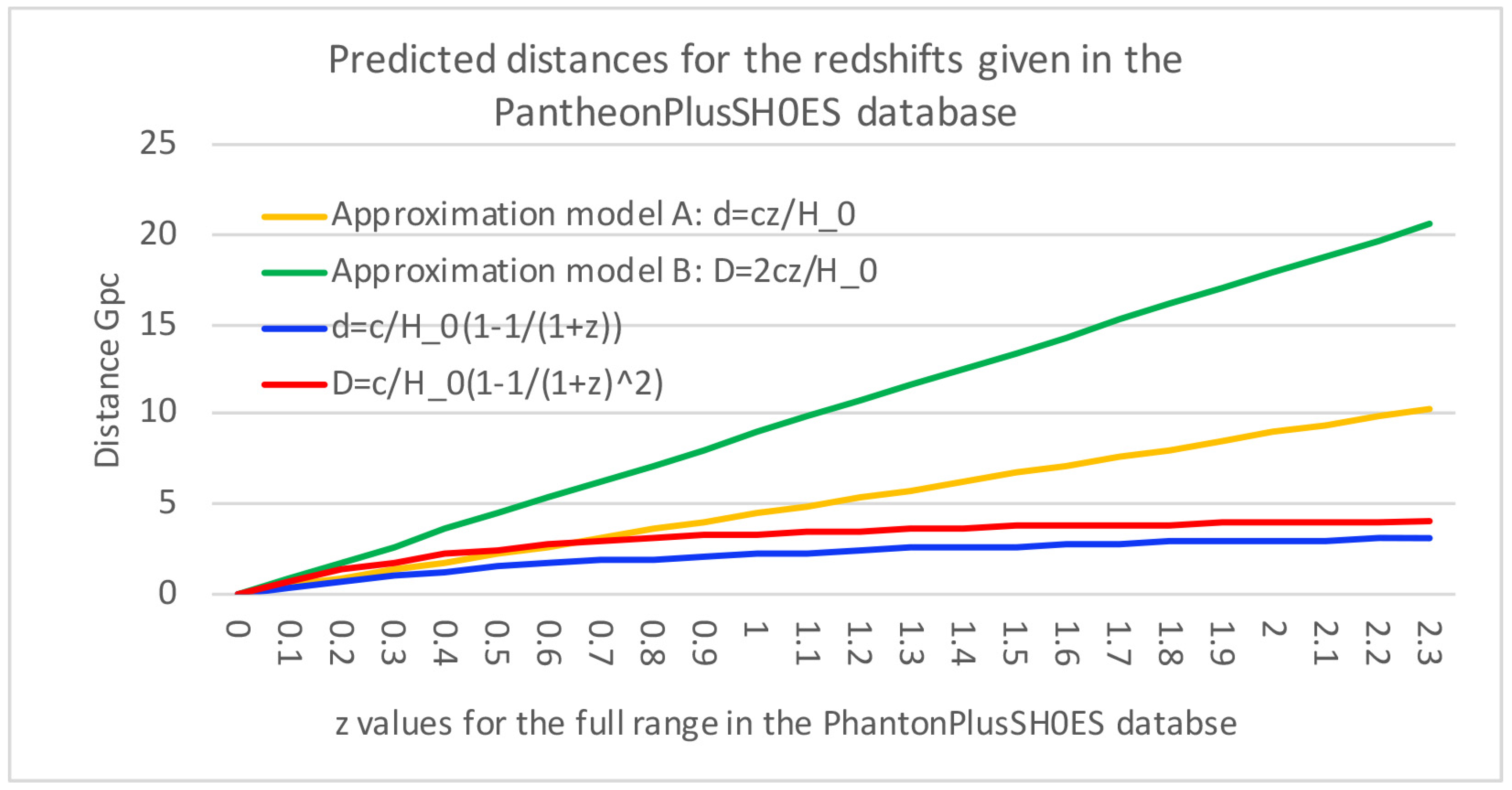
Figure 1 shows the predicted distances for the full z range in the PantheonPlusSH0ES supernova database. We have predicted the distances based on the two approximation formulas. The two approximation formulas are based on the first term of the Taylor series expansion and are, in reality, only good approximations when $z\ll 1$. This is why these approximations strongly overestimate the distances for high-z supernovae. The two exact solutions, based on the assumptions given in this paper, yield different values. The model consistent with $T_t=T_0(1+z)$ predicts a distance for each z as given by the red line. The model consistent with $T_t=T_0{(1+z)}^{1/2}$ predicts a distance for each z as given by the blue line. We will soon come back to comparing these distances with what is predicted from the $\Lambda$CDM model. We incorporate the current value of $H_0$ to make these distance approximations, which we take from the Particle Data Group [PDG] Astrophysical Constants and Parameters, which gives $H_0=67.4\pm 0.5 km/s/Mpc.$

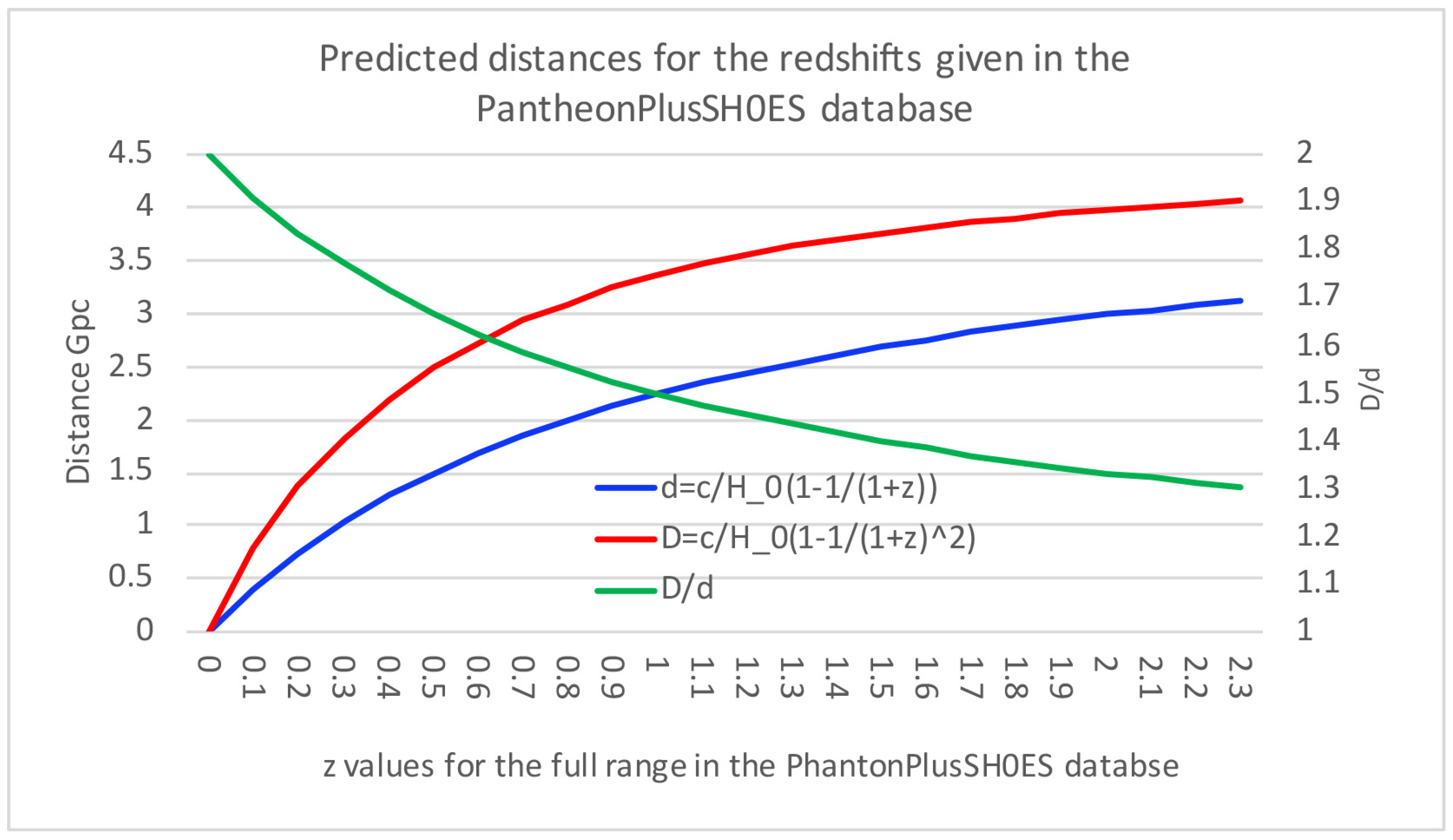
In Figure 2 we have removed the approximation models and we now focus on those models which are relatively more accurate at higher redshifts. This makes more obvious the difference between the model consistent with $T_t=T_0{(1+z)}^{1/2}$, and which we will now call Model A, and the model consistent with $T_t=T_0(1+z)$, which we will now call Model B. Be aware that the $\Lambda$-CDM model predicts the same distances as the blue line, at least for low z values. The red line prediction is what likely is correct, however, as it is consistent with $T_t=T_0(1+z)$, which we will show that observations seem to favor. This will become more clear in the next section. The green line represents $D/d$.

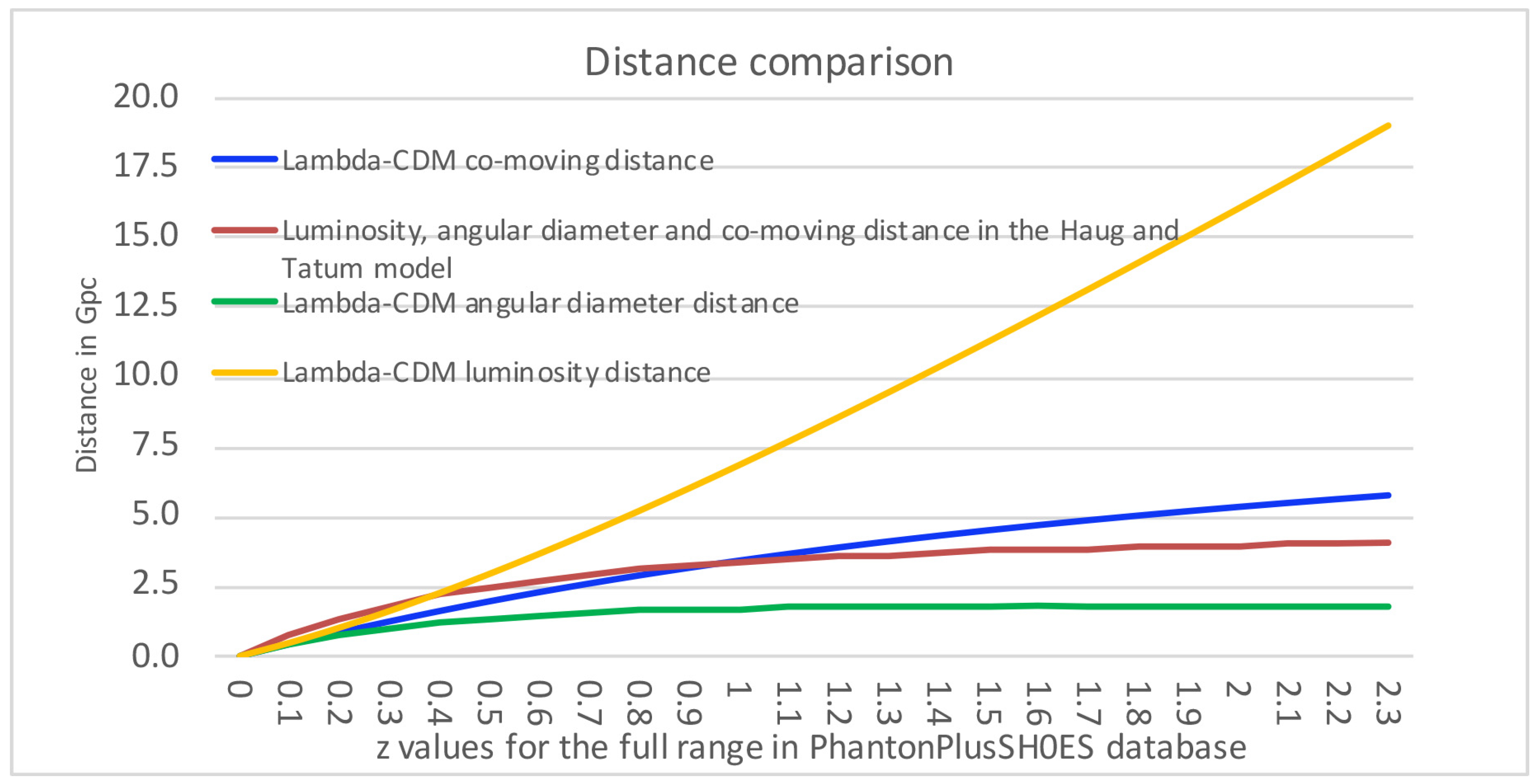
In Figure 3, we compare the predicted distance in our model for a given redshift with the three distances predicted by the $\Lambda$-CDM model. In the new model described in this paper, the co-moving, luminosity, and angular diameter distances become identical—a concept discussed in more detail in our recent paper [41]. Importantly, our model fully complies with Etherington’s [42] reciprocity theorem, which is based primarily on solid geometry and also plays an important role in the $\Lambda$-CDM model. Since none of the three distances predicted by the $\Lambda$-CDM model match the distance predicted by our model, none of these $\Lambda$-CDM distances can be used to verify the accuracy of our predicted distance.

The only independent method of distance determination potentially available is parallax. Parallax is highly robust and independent of any particular cosmological model; it is grounded in straightforward geometric principles but has, for practical reasons, been limited to very short cosmological distances. Hypothetically, parallax could be applied to distant galaxies and potentially also supernovae, but for such cases, standard parallax methods do not necessarily retain the same robustness. It is well known that standard parallax, if hypothetically applied to distant galaxies, would require redshift adjustments; thus, even parallax distance predictions for such distant objects would be influenced by the underlying model; see Hogg [43] .

We propose that the $\Lambda$-CDM model’s likely inaccuracy in predicting distances is the fundamental cause of the Hubble tension. In our model, the co-moving, luminosity, and angular diameter distances are unified into a single distance, not by assumption, but from derivations [41]. This unified distance feature, together with the rest of our model, appears to resolve the Hubble tension. As we will demonstrate, our model’s ability to predict all SN Ia redshifts with only one Hubble parameter is likely the most compelling evidence that our model also predicts the correct distances.

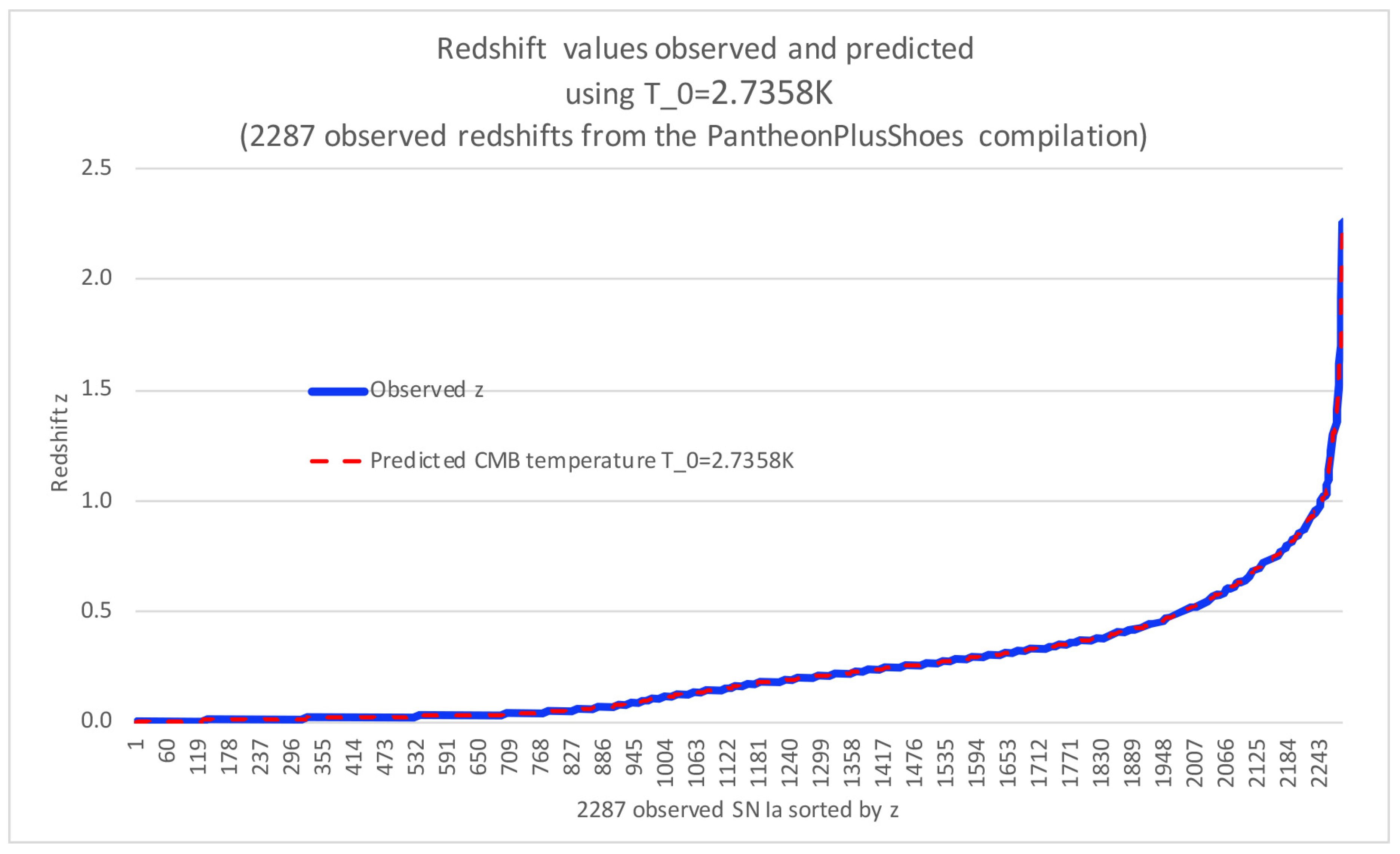
4. Extracting the Current CMB Temperature from 2287 Type Ia Supernovae

Here we use the observed redshifts from 2287 supernova data points in the PantheonPlusSH0ES database to determine the current CMB temperature ($z=0$). The methodology employed is as follows: from the cosmological redshifts, we first predict the CMB temperatures for each observed z value, by using the standard and well-known relation $T_t=T_0(1+z)$. Since our goal is to find $T_0$ a priori, we start with a wild guess. For instance, we might start with $T_0=4K$, or even $T_0=10K$, which is naturally far off from the currently observed CMB temperature of approximately $2.725K$. We start with a wild guess because we will later use optimization to determine if there exists a $T_0$ that leads to an estimation error near zero, using the redshift prediction formula $z=\sqrt{{\displaystyle \frac{R_h}{R_t}}}-1$. This can be achieved using optimization algorithms such as the Newton-Raphson method or the bisection method.

Next, we calculate the radius of the Hubble sphere going back in time for each z value. This is done by assuming a FSC-like $R_h=ct$ cosmology and solving Equation (2) for $R_t$. This gives:

$$R_t={\left({\displaystyle \frac{\hslash c}{T_t{k}_{b}4\pi }}\right)}^2{\displaystyle \frac{1}{2l_p}}$$

(25)

and since we also have $T_t=T_0(1+z)$, we can replace $T_t$ with this and get:

$$R_t={\left({\displaystyle \frac{\hslash c}{T_0(1+z)k_{b}4\pi }}\right)}^2{\displaystyle \frac{1}{2l_p}}.$$

(26)

Because we are assuming that we do not know $T_0$, we will not rely upon measured CMB temperatures. However, we can now input this expression for $R_t$ into our redshift formula (Equation (16)) and we get:

$$z_{pre}=\sqrt{{\displaystyle \frac{R_h}{R_t}}}-1=\sqrt{{\displaystyle \frac{R_h}{{\left(\frac{\hslash c}{T_0(1+z_{obs})k_{b}4\pi }\right)}^2\frac{1}{2l_p}}}}-1.$$

(27)

We can now minimize the errors between $z_{pre}$ and $z_{obs}$ by adjusting the unknown $T_0$ value. This can be accomplished through pure trial-and-error, or more efficiently by using “intelligent" trial-and-error systems such as the Newton-Raphson method or the bisection method. The results from these approaches are the same, except that, by naive trial-and-error, one will waste more time finding the optimal CMB temperature. To do this, we also need $R_H={\displaystyle \frac{c}{H_0}}$, which is the current Hubble radius, and therefore, we also need the current value of $H_0$, which we take from Particle Data Group [PDG] Astrophysical Constants and Parameters which gives $H_0=67.4\pm 0.5 km/s/Mpc$. Thus, $H_0$ affects the value; it is actually this relatively new theoretical relationship between the Hubble parameter and CMB temperature, first given by Tatum et al [1] in 2015 and later proved to be derivable from the Stefan-Boltzmann law by Haug and Wojnow [4,5], that makes this method possible. We also need the Planck length in our formula, so we have used the NIST CODATA (2018) value of $l_p=1.616255\times {10}^{-35}$ m (with standard uncertainty of $0.000018\times {10}^{-35}m$). This uncertainty is therefore reflected in the reported STD for both our predicted CMB temperature as well as our predicted $H_0$ using the PantheonPlusSH0ES database.

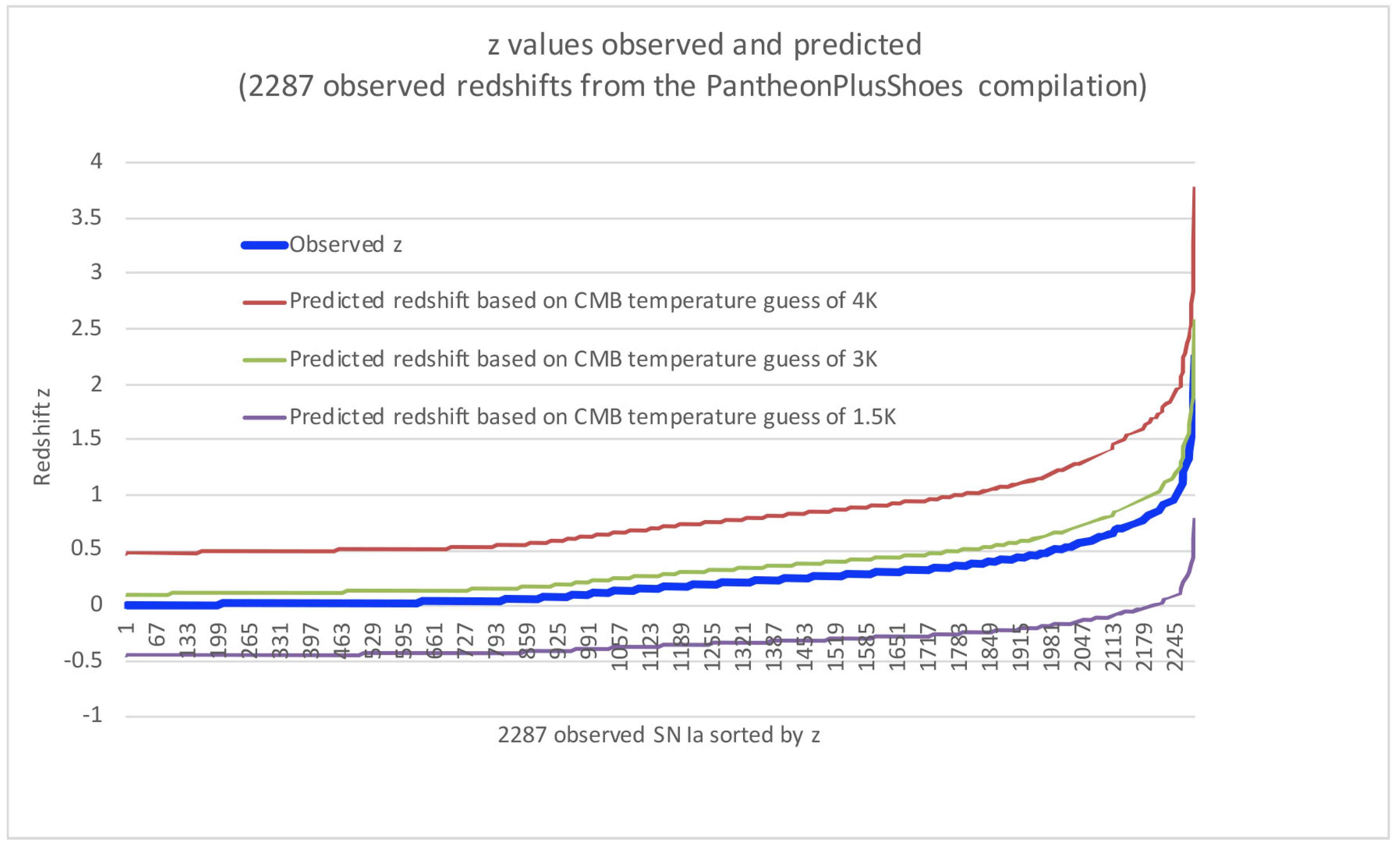
Figure 4 best illustrates the trial-and-error procedure. Assume that we initially have guessed a CMB temperature of $4K$. This is the red line in the figure, that we see is far above the observed redshifts represented by the blue line. However, at least it looks like it correlates well, and the measured Pearson correlation is actually a perfect ${\rho }_{obs,pre}=1$. This should not come as a big surprise, since we claim to have developed exact relations between z, $H_0$ and the CMB temperature. However, the output prediction is no better than the input prediction; the guess of CMB temperature $T_0=4K$ is way off. Given that the redshift predictions are proportional to the current CMB temperature, we must guess a lower CMB temperature. Assume that we now guess $T_0=1.5K$; we then get the predictions presented by the purple line. It becomes obvious that our $1.5K$ prediction is now too low compared to the observed redshifts. We now know that the CMB temperature needed in order to minimize the prediction errors must be between $4K$ and $1.5K$. We, therefore, now guess $3K$, and the redshift predictions we get from this (the green line) are much closer to observed, but still too high.

We can continue ‘manually’ like this, or we can resort to efficient search algorithms that are used for similar statistical problems in many scientific fields. Among the most commonly used algorithms are the Newton-Raphson method or the bisection method. One can also use the goal seek function in Excel, which is likely based on the bisection method. These trial-and-error methods are simply a form of calibration method. The question is whether there exists a single CMB temperature, denoted as $T_0$, for the current epoch of the cosmos that can make our “CMB redshift prediction formula” match the observed redshifts with precision.

Effectively, we are calibrating our new cosmological redshift prediction equation relative to the observed 2287 supernova redshifts by finding the value of $T_0$ that minimizes our prediction error. Only one parameter is adjusted (optimized), namely the "unknown" current CMB temperature, so that the errors indicated by the sum of ${\sum }_i^n\left({\displaystyle \frac{z_{pred,i}-z_{obs,i}}{z_{obs,i}}}\right)$ are minimized. This means that the sum of all individual redshift predictions is minimized by changing only one parameter, which in this case is the current CMB temperature $T_0$ in equation (27). This could potentially lead to a scenario where only the average error is zero, with some errors being positive and others negative, canceling each other out. However, we can easily check this after the optimization has been done by comparing all predicted redshift values individually against their corresponding observations. This is demonstrated graphically in Figure 5, where we can see that all predictions match their observations based on using the same optimized $T_0$ for all predictions. In other words, it is not only that the average error is low, but all of the individual errors are close to zero. That said, each prediction indirectly incorporates the observed redshift parameter, as can be seen from Equation (27), so this can indeed be labeled as a form of curve fitting. However, the important point is that our simple redshift function can easily match all observed redshifts using only a single free parameter, namely the CMB temperature in this case. Or, alternatively, we could choose the Hubble constant value as our free parameter (see below). This flexibility is based upon the duality we have discovered between $T_0$ and $H_0$ values.

To be even more precise on exactly how we minimize the errors, for all redshift observations we first calculate:

$$z_{pre,i}=\sqrt{{\displaystyle \frac{R_h}{R_t}}}-1=\sqrt{{\displaystyle \frac{R_h}{{\left(\frac{\hslash c}{T_0(1+z_{obs,i})k_{b}4\pi }\right)}^2\frac{1}{2l_p}}}}-1.$$

(28)

where $z_i$ is the observed redshift combined with an initial "wild" guess for the CMB temperature $T_0$. In addition, we need a measured $H_0$ value if we try to find the CMB temperature; all other inputs are known constants: $k_b$, c, ℏ, $l_p$ (where we also take into account the uncertainty in the Planck length $l_p$). This leads to predictions of all our redshifts that are far away from observed redshifts (see again Figure 4). Then, for each predicted redshift, we calculate the percentage error relative to the observed: ${\displaystyle \frac{z_{pre,i}-z_{obs,i}}{z_{obs,i}}}$. Then we sum up all of the errors. By trial and error, we only change $T_0$, and for each new intelligent guess on $T_0$, we repeat the procedure of recalculating all of the errors ${\displaystyle \frac{z_{pre,i}-z_{obs,i}}{z_{obs,i}}}$. We continue this trial and error process until we cannot reduce the sum of errors any further, and with a very high precision.

The only values we use from the PantheonPlusSH0ES SN Ia database are the redshifts. For each of the 2287 observed redshifts, we calculate $z_{pre,i}$ based on Equation (28) using a single guess of $T_0$, our free parameter in this case. We use the same guess of $T_0$ for all 2287 $z_{pred}$. All of the predicted values are then compared with the corresponding observed values. Statistically, for all 2287 predictions, we can then summarize the percentage error relative to the observations according to ${\sum }_{i=1}^{2287}{\displaystyle \frac{z_{pre,i}-z_{obs,i}}{z_{obs,i}}}$.

As we can see from Equation (28), if we reduce the guess of $T_0$, the predicted redshift values will go down, and if we increase the guess of $T_0$, the predicted redshift values will go up. This helps us to determine the direction to adjust $T_0$ to reduce the sum of errors ${\sum }_{i=1}^{2287}{\displaystyle \frac{z_{pre,i}-z_{obs,i}}{z_{obs,i}}}$. After making these adjustments several times, the errors are reduced to close to zero for all $z_{pre}$ simultaneously. This means that there is one best-fit $T_0$ value for all $z_{pre}$, which we now see in Figure 5. This result seems almost too good to be true. However, the reason that this is possible is that we are using a linear $R_h=ct$ model, where there are linear relations over cosmic time, unlike the $\Lambda$-CDM model, which has highly non-linear relations and lacks a formula to predict the CMB temperature in this way. Using Equation (28) in this way, anyone should be able to recreate our findings by inputting only the 2287 redshift values in the PantheonPlusSH0ES database.

This method does not in any way guarantee zero or close to zero error for any model. If the model is misspecified or simply not flexible enough to match all of the observed redshifts, then even after minimizing errors, there will be considerable error. This is clearly demonstrated in Section 8 where we illustrate exactly this point.

Of course, it is almost always possible to come up with a mathematical function with enough flexible variables that can be tweaked to match observations; this would be, in our view, pure curve fitting, which would obviously be of little value. On the other hand, our model is derived from foundational principles, such as the Stefan-Boltzmann law, and with no initial aim at matching observed redshifts. It is the CMB temperature formula of Eq. (1), combined with the observable confirmed relation: $T_t=T_0(1+z)$, that leads directly to our redshift prediction formula. We have not added additional factors in order to match redshifts. For example, one could have added extra parameters (extra degrees of freedom) to our model to allow for some form of dark energy. On the contrary, we find that our simple $R_h=ct$ model does not need any extra freedom parameter in order to match the full distance ladder of redshifts, while simultaneously matching the CMB temperature and being fully consistent with $T_t=T_0(1+z)$.

The approach of minimizing errors just described results in a predicted current CMB temperature $T_0\approx 2.73576067604891K$ from the 2287 supernova observations in the PantheonPlusSH0ES database. We are not claiming that the current CMB temperature is exactly this (although it could be); rather, this is what it appears to be, based on the observed supernova redshifts in combination with the $H_0=67.4km/s/Mpc$. When we also take into account the uncertainty in the value of $H_0$ ($67.4\pm 0.5km/s/Mpc$), as reported by the Particle Data Group [PDG] Astrophysical Constants and Parameters, we get a one standard deviation (STD) confidence interval range of $2.7256K$ to $2.7459K$ for the current CMB temperature; the 95% confidence interval is $2.7154K$ to $2.7560K$. The reason we provide the numerous digits in $T_0\approx 2.73576067604891K$ is simply to enable others to obtain the same value when utilizing $H_0=67.4km/s/Mpc$ following the procedure outlined in this paper. This is not meant to imply that we can determine the CMB temperature with such high precision. The measured CMB temperature has a lower uncertainty compared to our predicted CMB temperature. Rather, what is important to understand here is that we have a model that directly links the current CMB temperature to the Hubble constant. To the best of our knowledge, the $\Lambda$-CDM model does not offer such a direct relationship between the current CMB temperature and $H_0$.

As different Hubble constant measurement studies and methods yield considerable uncertainty in $H_0$, this uncertainty could be even larger. Moreover, there is the heretofore unexplained Hubble tension problem; see for example [44,45,46]. Nevertheless, using our new radically-different theoretical approach, we can closely approximate the recent CMB temperature observations by [47,48,49,50].

By assuming a current CMB temperature $T_0=2.7358{\pm }_{0.0102}^{0.0101}K$, the predictions from Equation (27) are now perfectly aligned with the observational blue line in Figure 5. In other words, the redshift formula we have presented is now capable of matching observed cosmological redshifts, if we start out with a measured CMB-based Hubble constant value.

It is interesting that, by incorporating only the current CMB temperature and Hubble constant value, our redshift prediction function can match observations. It is important to note that we are matching the same epochal $T_0$ for all supernovae, rather than different $T_0$ values for different supernovae. We must keep in mind that all such redshifts have been measured in the current CMB temperature epoch. This basically demonstrates that our framework is consistent and robust. Our findings are fully consistent with the empirically-tested relation $T_t=T_0(1+z)$ and also with the FSC growing black hole variant of $R_h=ct$ cosmology. It is our recommendation that the astrophysics community pay attention to this result and investigate to what degree it is or is not consistent with the $\Lambda$-CDM model. Could it be that the $\Lambda$-CDM model needs further adjustments? Or could it be that $R_h=ct$ models are actually more realistic in some respects? Only further research can settle these questions. In either case, researchers should be made aware of the recent progress in our theoretical understanding of CMB temperature and its relationship to cosmological redshift and the Hubble constant.

5. Why We Think That We May Have Solved the Hubble Tension Problem

In the section above, where we found the CMB temperature that optimally fits with the observed supernova redshifts, we had to know the Planck-derived Hubble constant value. Alternatively, one can use the observed CMB temperature to optimally fit a Hubble constant value for the same 2287 supernova redshifts. The CMB temperature has been extremely accurately measured in recent years, for example, by [47,48,49,50].

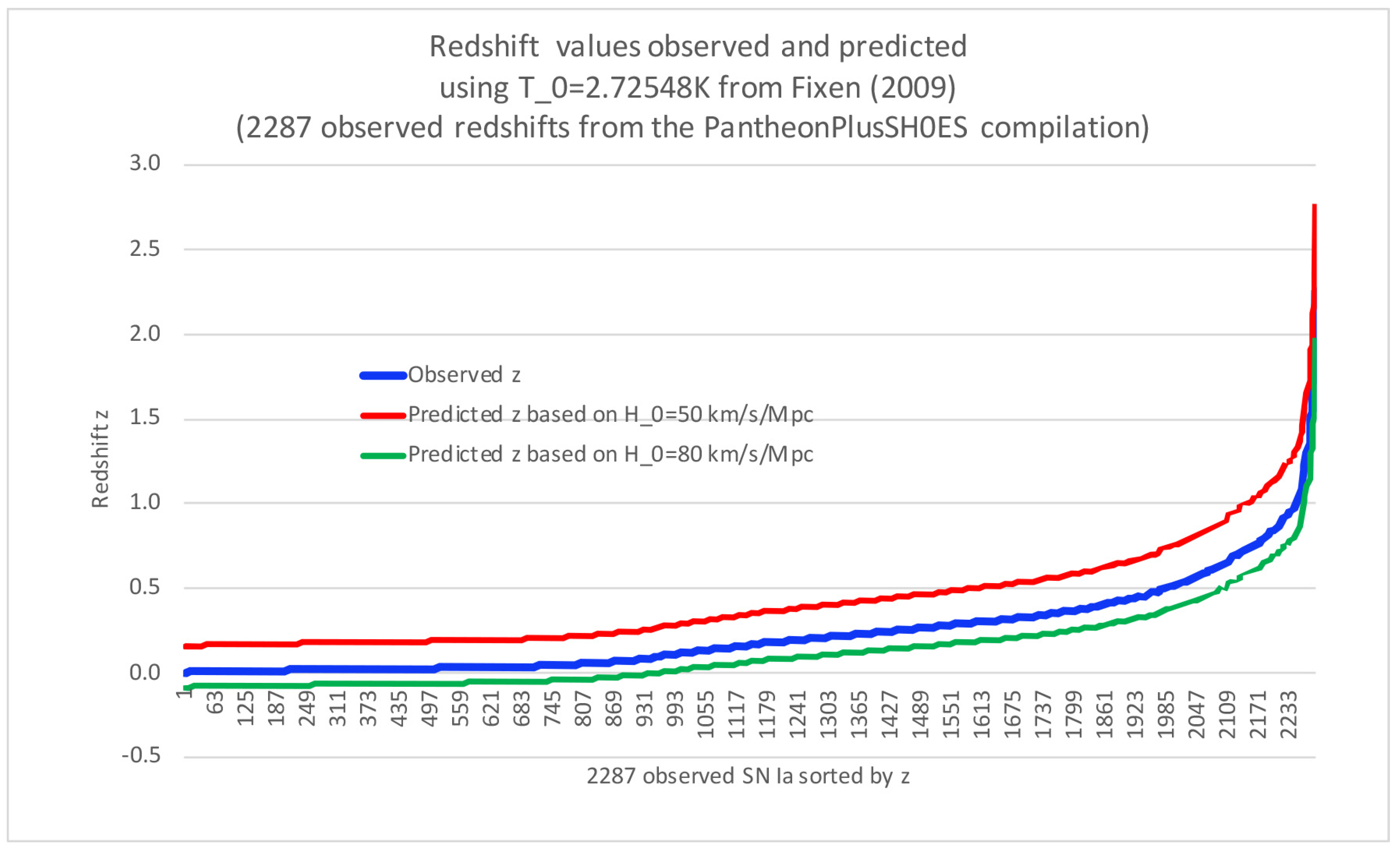
First we will use the most recent measurement by Fixen (2009) [48], a CMB temperature of ${2.72548}_{-0.00057}^{+0.00057}K$, which is also fully consistent with the Particle Data Group (PDG)3 Astrophysical Constants and Parameters that suggest $T_0={2.7255}_{-0.0006}^{+0.0006}K$. We then start out by assuming that we know very little about the Hubble constant value. All we know is that many different studies have arrived at different values. So we start with a qualified, but wild, guess that it must be in a range from 50 to $80 km/s/Mpc$. We then ask if there is a single Hubble constant $\left(H_0\right)$ value that, when used in our new CMB redshift prediction formula, matches all of the observed supernova redshifts. So, we start with a guess of $H_0=50 km/s/Mpc$ and use the same formula as in the previous section:

$$z_{pre}=\sqrt{{\displaystyle \frac{R_h}{R_t}}}-1=\sqrt{{\displaystyle \frac{R_h}{{\left(\frac{\hslash c}{T_0(1+z_{obs})k_{b}4\pi }\right)}^2\frac{1}{2l_p}}}}-1.$$

(29)

The only difference in our approach (compared to in the previous section) is that we now substitute the CMB temperature measured by Fixsen (2009) for $T_0$. In the previous example, we assumed that we knew $H_0$ and tried to find $T_0$. We can now use $R_h={\displaystyle \frac{c}{H_0}}$ to solve for $H_0$.

See Figure 6. Once again, the actual observed redshifts for all 2287 supernovae in the PantheonPlusSH0ES database are represented as the blue line. As we can see, the red line indicates that this was an underestimated Hubble constant value, as our redshift prediction formula is inversely related to $H_0$. Accordingly, we next guess a much higher Hubble constant value, for example $H_0=80 km/s/Mpc$, which gives redshift predictions correlating to the green line. Now the redshift predictions are too low. By simple trial-and-error, or by "intelligent" trial-and-error methods, such as the Newton-Raphson method or the bisection method, we can find the $H_0$ that minimizes the errors between predicted and observed redshifts.

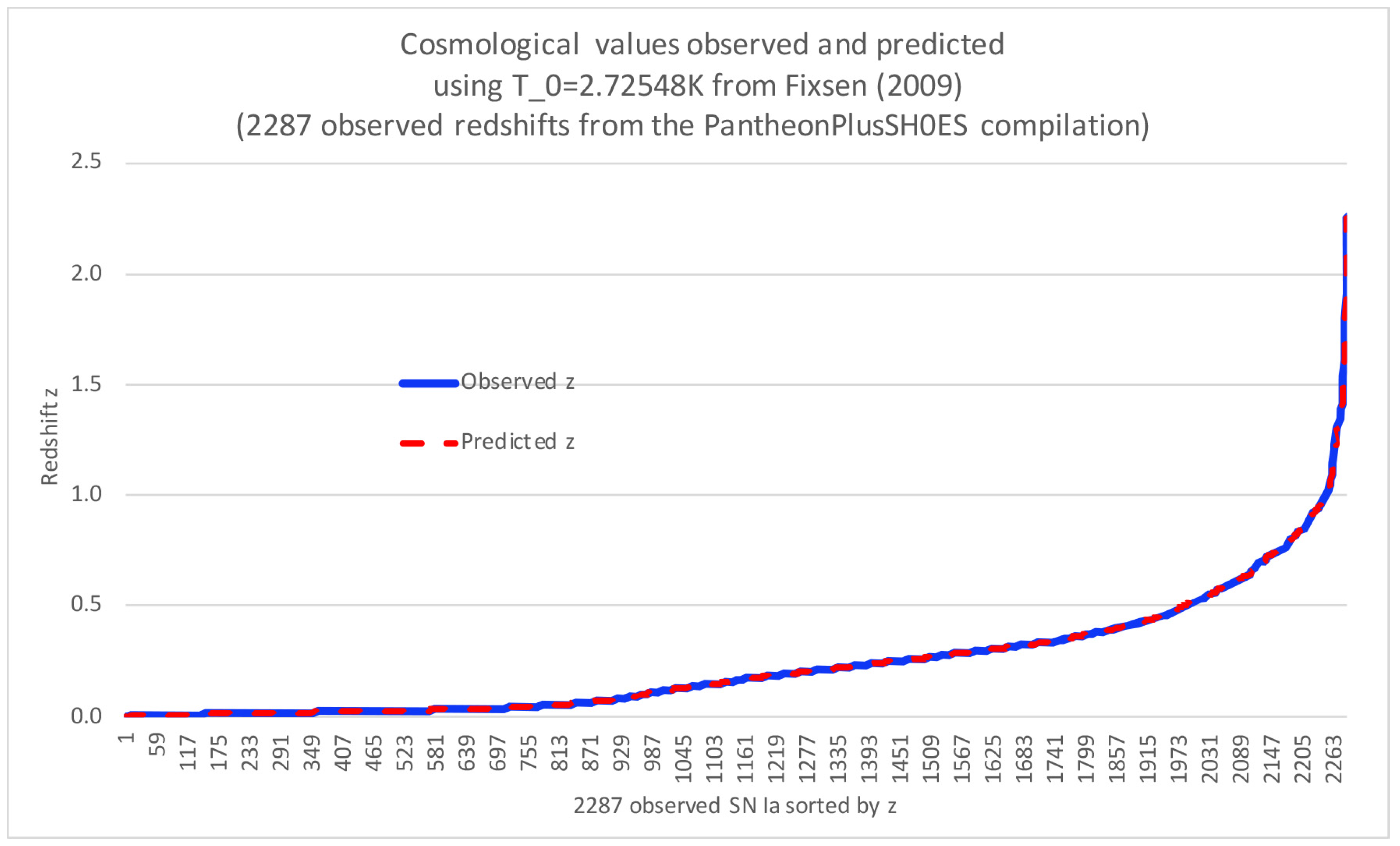
Figure 7 shows the end-result. Here we are using the Fixen (2009) CMB temperature of ${2.72548}_{-0.00057}^{+0.00057}K$. From this, in combination with the 2287 supernovae PhantonPlusSH0ES redshift data, a best fit is achieved with $H_0={66.8943}_{-0.0287}^{+0.0287} km/s/Mpc$ (corresponding to a 1STD range of $66.8656$ to $66.9230 km/s/Mpc$). This is well inside the 95% confidence interval given by the Particle Data Group [PDG] Astrophysical Constants and Parameters, which gives $H_0=67.4\pm 1 km/s/Mpc$ for the 95% confidence interval. This trial-and-error methodology has recently been validated with a closed form solution (see Haug [51]) to the Hubble tension based on the same underlying Haug and Tatum cosmology model presented herein. This gives us great confidence in our methodology and in an actual duality between $T_0$ and $H_0$.

Here, it is important to be aware that we are able to achieve essentially a perfect fit with all of the PantheonPlusSH0ES database supernovae using either a single measured Hubble constant value or a single measured CMB temperature. This appears to us to solve the Hubble tension problem in favor of the Planck Collaboration Hubble constant determination. The Hubble constant value cannot be measured directly; it is the redshift that is measured in the incorporated type Ia supernova studies. The Hubble constant is estimated, and therefore relies on a model-based definition of redshift. In this paper, we use a new redshift model rooted in our new understanding of the inter-relationships between the current CMB temperature, the current Hubble constant, and cosmological redshifts; see [1,4,52]. This approach is clearly consistent with black hole variants of $R_h=ct$ cosmological models. Whether it can also be made compatible with the $\Lambda$-CDM model is too early to say. If so, we believe that the $\Lambda$-CDM model, at minimum, would need some adjustments. Alternatively, it may be that such $R_h=ct$ model variants are actually more realistic.

Our results are also fully in-line with the recent findings of Tatum et al [53] that one can accurately find $H_0$ from knowing the current CMB temperature, or vice-versa, something which the $\Lambda$-CDM model cannot do at present, as far as we know. Herein, we have taken an additional step forward and linked these two cosmological parameters to cosmological redshift. These inter-relationships are consistent with core principles in such $R_h=ct$ cosmology model variants in general, and FSC in particular.

In retrospect, the PantheonPlusSH0ES dataset relied upon in this paper appears to be particularly useful in solving the Hubble tension problem. Firstly, it is a rich dataset of 2287 type Ia supernova redshifts spanning the astronomical distance ladder, all of which have been incorporated into our parameter-matching algorithm. Our use of so many data points, in conjunction with the modern precision in measuring the CMB temperature, undoubtedly contributes to the remarkably low uncertainty in the derived (i.e., matched) Hubble constant values given above. This speaks to the power of using a carefully designed method, as employed herein. Furthermore, it speaks to the robust nature of our methodology that we have used the “local universe” dataset of supernova redshifts to severely challenge the reliance of other recent local universe studies upon the remote astronomical distance ladder for Hubble constant determination. The Riess et al SH0ES studies, for instance, have relied heavily on correct calibrations of the astronomical distance ladder for their Hubble constant determination accuracy. We believe that our Hubble constant, cosmological distance, and redshift formula comparisons in Section 2 and Section 3, particularly with reference to equation (9) of standard cosmology and equation (18) derived within our $R_h=ct$ cosmology subclass, have much to do with solving this tension. The text following equation (23) and preceding the Figure 1 description can be regarded as the crux of this paper.

It is also important to ask what the dataset of baryonic acoustic oscillations (BAO) might reveal with respect to our Hubble tension solution. With respect to BAO data, Melia has extensively evaluated different cosmological models in comparison to the linear $R_h=ct$ model. His recent study [54] of BAOs in the Lyman-alpha forest at an effective redshift of 2.334 concludes that the results are “completely consistent with the cosmic geometry predicted by$R_h=ct$.” He further points out that the results also provide “strong evidence disfavoring the standard model.” Melia’s work has demonstrated other successes of linear $R_h=ct$ models in comparison to $\Lambda$-CDM with respect to observational data; see, for instance, [55].

In summary, we conclude that the Planck Collaboration Hubble constant value of $67.4\pm 0.5 km/s/Mpc$ [56] is strongly supported by the PantheonPlusSH0ES supernova redshift dataset. We also conclude that the Riess et al SH0ES study Hubble constant value of $73.04\pm 1.04 km/s/Mpc$ [57] is strongly disfavored by the PantheonPlusSH0ES supernova redshift dataset, at least within $R_h=ct$ cosmology. Nevertheless, ongoing studies and comparisons of the different models are recommended. Murakami et al. [58] have recently improved their estimate of $H_0$ using the full distance ladder of Type Ia supernovae (SN Ia) to determine $H_0=73.01\pm 0.92 km/s/Mpc$. Although this is impressive within the mathematical lens of the $\Lambda$-CDM model, we must conclude that our new approach to examining cosmological redshifts in relation to CMB temperature does not align with this value when also utilizing the full distance ladder of SN Ia redshifts in conjunction with our $R_h=ct$ model. In sharp contrast, we obtain a value of $H_0={66.8943}_{-0.0287}^{+0.0287} km/s/Mpc$. While we do not expect this to be automatically accepted, we hope that our results will encourage other research groups to closely examine our new cosmological model, which is consistent with the $R_h=ct$ principle and seems to resolve the Hubble tension in addition to reducing uncertainty in the $H_0$ value compared to other models and methods.

There are also other types of observations not discussed in this study. For example, de Jaeger et al. [59] also estimate $H_0$ from SNe II. However, they have correctly pointed out that, unlike SN Ia, “the SNe II are not standard candles,” and therefore, they have to be standardized through theoretical or empirical methods as pointed out by the authors of that study. A database of SNe II observations is clearly something that also could be of interest to explore within our model framework, but it falls outside the scope of our current paper, and we strongly doubt that it would change our conclusions if pursued. However, we suggest it here as yet another dataset one can investigate with this method. We have first chosen SN Ia observations, simply because they are known as our best standardized candles, covering the full distance ladder.

6. Cosmic Evolution

Cosmic evolution in $R_h=ct$ cosmology has been discussed in considerable detail by Melia [60]. Melia points out that “As of today, more than 27 different kinds of observation have been used in comparative studies between this model and Λ-CDM, at both high and low redshifts, employing a broad range of integrated and differential measures, such as the luminosity and angular diameter distances, the redshift-dependent expansion rate, and the redshift-age relationship. In all of the tests completed and published thus far, $R_h=ct$ has accounted for the data at least as well as the standard model, and often much better.”

Melia [61] has recently noted that observations from the James Webb Space Telescope (JWST) strongly support the $R_h=ct$ cosmology timeline and severely challenge the timeline predicted by $\Lambda$-CDM. Melia’s findings align well with the $R_h=ct$ cosmological model presented herein, which also predicts an age of the universe of 14.6 billion years [62].

In our solution to the Hubble tension under $R_h=ct$ cosmology, we obtain $H_0={66.8943}_{-0.0287}^{+0.0287}$$km/s/Mpc$, which corresponds to an age of the universe of 14.6 billion years. This provides approximately 800 million years more than the $\Lambda$-CDM model, potentially explaining why early galaxies appear to be so well-formed at the great distances observed by the James Webb Space Telescope. For a detailed discussion, see Haug and Tatum [63]. The ongoing debate in the literature about the advantages and disadvantages of various cosmological models is essential for scientific progress. Given the recent developments, we firmly believe that it is too early to draw definitive conclusions; further investigation is necessary. In this spirit, the present paper contributes additional insights into $R_h=ct$ models, specifically focusing on a promising version of the $R_h=ct$ model which appears to resolve the Hubble tension.

We have already derived quantities such as the radiation density from our model [64] and obtained ${\Omega }_{\gamma }={\rho }_{\gamma }/{\rho }_{crit}\approx 5.53\times {10}^{-5}$, which lies well within the 95% confidence interval for the radiation density reported by the Particle Data Group (PDG), where the 95% confidence interval is $5.08$ to $5.68$ ($5.35\pm 0.15$ for 1STD). Our radiation density value is derived from the Friedmann equation in its recent thermodynamic form [63] linking it to the HTC type $R_h=ct$ model. Precisely how multiple new derivations from our model should be interpreted physically in cosmological evolution remains open to discussion, but the most important point at this stage is that the predictions from our model which we have examined so far appear to fit observations very well. There are still many open questions concerning our model, and we believe that only extensive research along the lines of our model over time can provide a final conclusion as to whether this model is truly preferable over others. So far, it appears extremely promising in addressing the Hubble tension and a series of other things, such as giving a possible explanation of the surprisingly-mature early galaxy formation observations by JWST [65]

An open question within the $R_h=ct$ model, as discussed in this paper, is the matter and energy content at different epochs of the universe. Whether these can be precisely predicted within this model remains unclear and requires further investigation. However, what we have derived and looked at so far in our model appears to be consistent with observational data. Recently, we published a brief comparison of our predicted Hubble parameter and predicted distances to objects over the cosmic evolution at the full distance ladder of z values from 0 to 2 provided in order to compare it to to the six different redshift bins used in the pending final DESI BAO study report; see Tatum and Haug [66] for more details.

7. Has Our Solution to the Hubble Tension Provided Us with New Universal Laws of Cosmology?

Figure 7 seems almost too good to be true. There may be a tendency to react in such a way, but the math appears to indicate otherwise. One even wonders if there are ‘new universal laws of cosmology’ revealed by such an approach, because there appear to be exact relationships between the Hubble constant, cosmological redshift and the CMB temperature, without requiring such concepts as dark energy acceleration and superluminal space-time expansion.

Naturally, it is not for us to say whether we have discovered ‘new universal laws.’ But we do wonder about this. Clearly, we have not simply found broad statistical correlations between these parameters, but rather very precise mathematical inter-relationships between them. If one knows any two of these cosmological parameters with high precision, one can automatically solve for the other with high precision. To take but one example, if one knows the CMB temperature and the Hubble constant, one can precisely estimate the cosmological redshift for a given cosmological distance. There is hardly any wiggle room. We find that a convenient way to illustrate this is in Figure 8.

The formula in the middle of the triangle demonstrates that the Hubble constant and the CMB temperature are simply connected by a composite constant that we have called Upsilon (the Latin symbol for Upsilon4): $\Omega ={\displaystyle \frac{k_b^{2}32{\pi }^2{G}^{1/2}}{c^{5/2}{\hslash }^{3/2}}}$. When we ponder these inter-relationships, we are left asking if the Lambda-CDM model can accommodate them, or whether they are appropriate for a new paradigm represented by such $R_h=ct$ model variants in general, and the FSC model in particular. We leave this question for others to ponder as well. It is worth mentioning that our model framework here is also consistent with a new thermodynamic approach to rewriting the Friedmann equation, which is fully consistent with the general theory of relativity; see again [63] and also [67].

8. Additional Comments Concerning Models and Analytic Methods Used

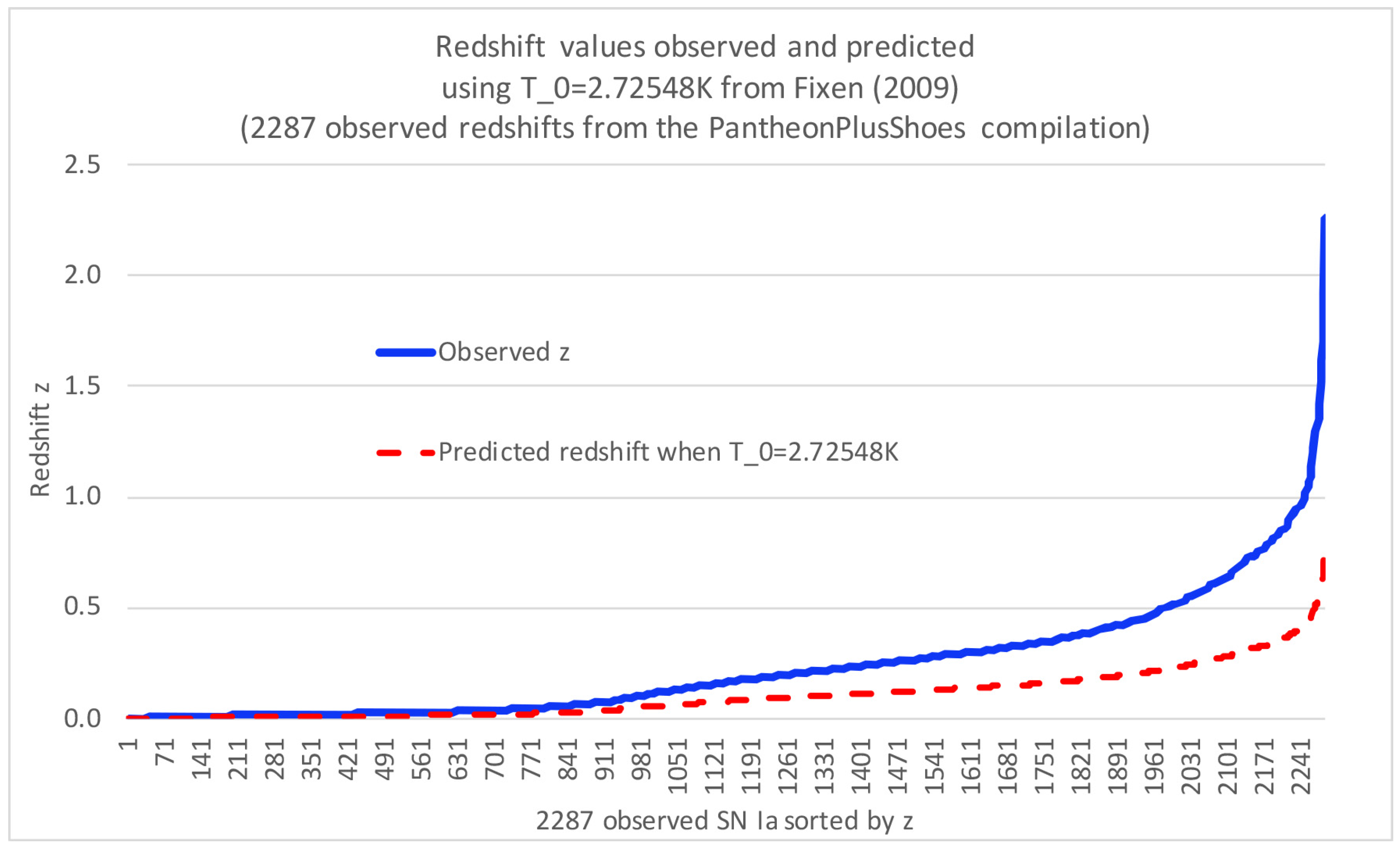
In addition to our particularly useful Model B, Model A can be similarly explored, but only if one accepts $T_t=T_0{(1+z)}^{{\displaystyle \frac{1}{2}}}$, which contradicts observational studies of z versus CMB temperature.

One could also consider a hypothetical case where $z=\sqrt{{\displaystyle \frac{R_h}{R_t}}}-1$ and $T_t=T_0{(1+z)}^{{\displaystyle \frac{1}{2}}}$. Figure 9 illustrates the observed versus predicted redshifts, when assuming this and a current observed CMB temperature of 2.72548K (again from Fixsen (2009). Here, we no longer have exact relationships that hold in practice, but merely statistical relationships. The resulting Pearson correlation coefficient between predicted and observed temperatures is $0.99813$, indicating a high correlation, but only a correlation and not an exact relationship. Furthermore, without the exact relationships that we propose, optimization with methods like Newton-Raphson or bisection would indeed not work as well. In such case, considerably better error minimization between observed and predicted temperatures could be achieved by using a more advanced parameter optimization method, such as Markov Chain Monte Carlo (MCMC). However, regardless of the quality of the parameter optimization methods, they would still fail to match results when exact relationships, instead, exist between $H_0$, z and CMB temperature, as proposed in the present paper. Ultimately, even after MCMC optimization, one would still need to explain the gaps between predicted and observed redshifts by introducing additional hypotheses on top of the existing model, such as dark energy causing an accelerated universe different from the $R_h=ct$ model. However, such is not necessary in order to match supernova redshift observations when the relationships between these parameters are as given and demonstrated in our Model B in the sections contained herein.

Of course, we do not exclude the possibility that dark energy exists in the universe and may be necessary in a ‘final’ model to explain other types of observations. We merely point out in this particular paper that our Model B is capable of matching all observed redshifts without relying upon a dark energy accelerating expansion of the universe.

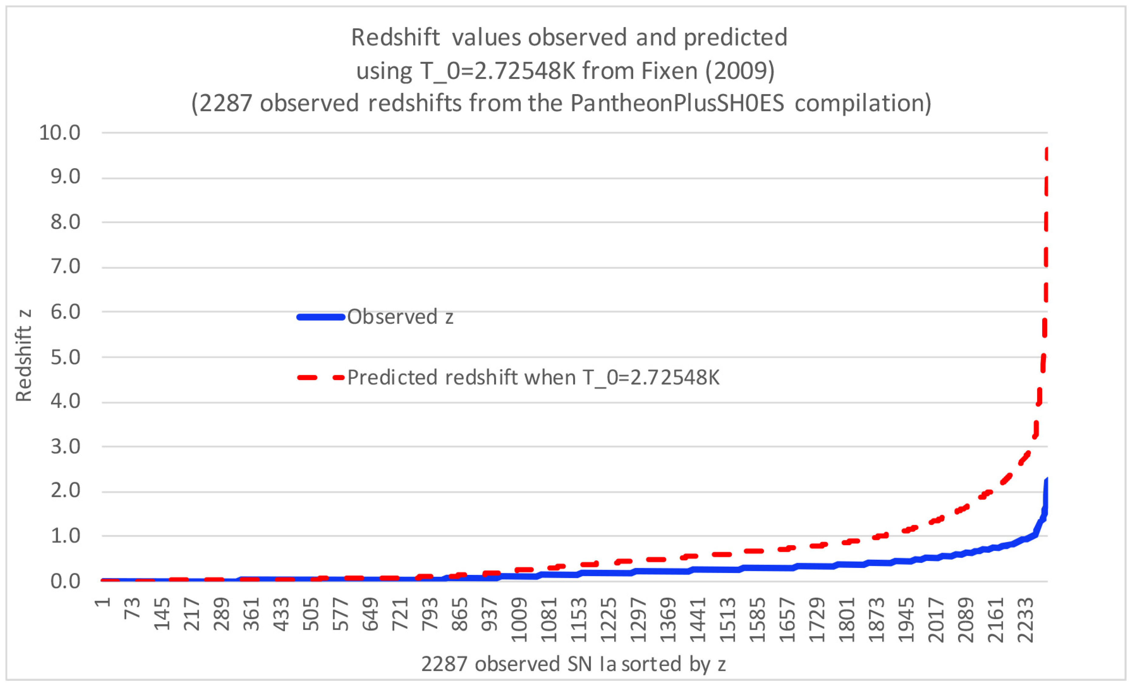
Figure 10 presents a suboptimal $R_h=ct$ model where the redshift is defined as $z={\displaystyle \frac{R_h}{R_t}}-1$ and $T_t=T_0(1+z)$. The Pearson correlation between predicted and observed values is $\rho =0.99211$. Optimization methods such as MCMC could potentially bring the predictions closer to the observed values, but achieving a ’perfect’ match, as we have demonstrated in previous sections, is unattainable because the model is inconsistent with reality. Without knowledge of better models, one might in this model be tempted to propose a new type of exotic energy that decelerates the universe to align with observations. This is in sharp contrast to the immediately preceding model. However, as we have clearly shown with our Model B in previous sections, such ad hoc adjustments are unnecessary. We can match the supernova redshifts perfectly if the model in question is better able to capture the reality, which we believe we get from $z=\sqrt{{\displaystyle \frac{R_h}{R_t}}}-1$ in combination with $T_t=T_0(1+z)$, which we call Model B.

9. Conclusions

In the context of growing black hole $R_h=ct$ model variants, we now have a robust theoretical framework for predicting the Cosmic Microwave Background (CMB) temperature by using a known Hubble constant value, or vice versa [1,5,53]. This can be done both for present and past cosmic epochs (presumably), as well as in relation to cosmological redshifts. This framework initially emerged from the FSC cosmological model proposed by Tatum et al. However, it is worth exploring whether it can also be applied to other black hole $R_h=ct$ models. The theory appears to be compatible with the relationship $T_t=T_0{(1+z)}^{1-\beta }$, but only when $\beta =0$ or $\beta ={\displaystyle \frac{1}{2}}$. Although it appears that we are gaining a new perspective on understanding and investigating cosmological redshift, further theoretical and observational studies are needed in order to reach a final consensus. There is still much to be discovered.

In this paper, we have demonstrated, from the observed redshifts of 2287 type Ia supernovae (the PantheonPlusSH0ES database), how to achieve a perfect match between a particular Hubble constant value $H_0$ and a $T_0$ value from a high precision CMB study. We refined our predictions by minimizing errors in our redshift prediction formula relative to the observed redshifts from the same 2287 type Ia supernovae. To give a prime example, utilizing the CMB temperature from Fixen (2009) of $T_0={2.72548}_{-0.00057}^{+0.00057}K$, we derive a Hubble constant value from the full supernova database of $H_0={66.8943}_{-0.0287}^{+0.0287} km/s/Mpc$. Remarkably, our redshift formula can accurately predict the redshift of every supernova in the PantheonPlusSH0ES supernova database after calibration for distance. While this process resembles curve-fitting, the only free parameters are either the Hubble constant or the CMB temperature, with one being derived from measurement and the other automatically determined as a result. These results are consistent with the predictive power mentioned in references [52,53]. Accordingly, we believe that our new approach has likely resolved the Hubble tension problem in favor of the Planck-based CMB-derived Hubble constant value. Nevertheless, our work should undergo careful scrutiny by others before drawing any lasting conclusions.