
Submitted:
03 January 2024
Posted:
04 January 2024
You are already at the latest version
Abstract
The pursuit of more efficient transport has led engineers to develop a wide variety of 1 aircraft configurations with the aim of reducing fuel consumption and emissions. However, these 2 innovative designs introduce significant aeroelastic couplings that can potentially lead to structural 3 failure. Consequently, aeroelastic analysis and optimization has become an integral part of modern 4 aircraft design. In addition, aeroelastic testing of scale models is a critical phase in aircraft devel- 5 opment, requiring accurate prediction of aeroelastic behaviour during scale model construction to 6 reduce costs and mitigate risks associated with full-scale flight testing. Achieving a high degree of 7 similarity between the stiffness, mass distribution and flow field characteristics of scaled models 8 and their full-scale counterparts is of paramount importance. However, achieving similarity is 9 not always straightforward due to the variety of configurations of modern lightweight aircraft, as 10 identical geometry cannot always be directly scaled down. This configuration diversity has a direct 11 impact on the aeroelastic response, necessitating the use of computational aeroelasticity tools and 12 optimization algorithms. This paper presents the development of an aeroelastic scaling framework 13 using multidisciplinary optimization. Specifically, a parametric Finite Element Model (FEM) of the 14 wing is created, incorporating parameterisation of both thickness and geometry, primarily using 15 shell elements. Aerodynamic loads are calculated using the Doublet Lattice Method (DLM) em- 16 ploying twist and camber correction factors, and aeroelastic coupling is established using infinite 17 plate splines. The aeroelastic model is then integrated within an Ant Colony optimization (ACO) 18 algorithm to achieve static and dynamic similarity between the scaled model and the reference wing. 19 A notable contribution of this work is the incorporation of internal geometry parameterisation into 20 the framework, increasing its versatility and effectiveness.
Keywords:
Aeroelasticity
; Structural optimization
; Low-fidelity aerodynamics
; Aeroelastic scaling
; Sizing optimization
; Layout optimization
1. Introduction
1.1. Motivation
Nowadays, the continuously search for climate-friendly transportation has led engineers to explore in-depth the design space and achieve more efficient configurations in order to reduce emissions, since aviation has a significant impact on climate change through the release of nitrogen oxides, water vapour, sulphate and soot particles at high altitudes [1]. The current objective is to reduce emissions at least 55% by 2030 compared to 1990 in order to become climate neutral by 2050 [2]. So, ensuring sustainable and efficient aviation is imperative with, the aerospace scientific community striving towards fulfillment of these goals. A way among others to reduce emissions is to design aircrafts pertaining a high Aspect Ratio (AR). The Induced Drag Coefficient, , is inversely proportional to AR, hence, wings designed with the highest possible AR enable induced drag reduction, which in turn cascades into less fuel consumption [3]. This trend is clearly illustrated in the subsequent Figure 1, where an increase in the AR of transport airliner wings is observed in the past decade.
Increasing AR is a great way to improve aerodynamic efficiency. However, from the structural discipline perspective the design of such structures proves to be a challenging task. In fact, high AR wings are more sensitive in bending and torsion due to their long span, thus, introducing non-linearities and aeroelastic effects. So, the study and analysis of those effects is a primary goal during the design of this type of aircraft wings in order to achieve a safe structure. Aeroelasticity investigates the interaction of aerodynamic, elastic and inertial forces acting on an aircraft and how this interaction impacts aircraft design and performance. High AR wings are structurally flexible and the deformation of the wing induces greater aerodynamic forces causing more structural deformations and this phenomenon continues in a closed loop till a condition of stable equilibrium is reached or the structure diverges and collapses. Aeroelastic phenomena can be categorized into two major divisions. First, the static aeroelastic where the inertial forces are negligible and the interaction between aerodynamic forces and elastic forces is investigated. Static aeroelastic deformations are important because they determine the lift and drag distribution, control surface effectiveness, trim performance and stability at steady flight conditions. Second, dynamic aeroelasticity also accounts for the inertial forces that are not negligible, and they influence the response of the aircraft. The main dynamic aeroelastic phenomenon is flutter which can be defined as the dynamic instability of an elastic body in airstream due to the interaction of stiffness, inertial and mass forces. Aeroelasticity is now seen as one of the key disciplines in design, and as one of the "critical" processes in the aircraft development approach [5]. Because of the significance of those phenomena, a plethora of methods to predict them has been developed. Prediction methods are divided into three categories, the development of computational and analytical methods, wind tunnel experiments on aeroelastically scaled models and the flight test of full-scale models. Engineers used to design aircrafts under extreme simplifying assumptions in order to avoid instabilities, but today’s lightweight and flexible designs could lead to catastrophic consequences. Things have changed due to the high cost and high risks of the flight test combined with the rapid development of computing power. This method is roughly used in recent years while a combination of computational aeroelasticity methods during the design phase with wind tunnel test of aeroelastic scaled models and a small number of flight tests. The approach that is currently used is depicted in Figure 2.
Aeroelastic scaling is mainly used for the in-flight testing of new designs, in order to reduce development costs, time and risks of manufacturing and testing the actual full-scale aircraft. An additional application of scaling is the testing of next generations of existing aircrafts. Stiffness distribution, mass distribution and aerodynamic loads may vary from generation to generation (e.g. engine mass, winglets control surfaces, fuel tanks etc.). With the use of scaled models, engineers can detect problems in the flight behaviour of the aircraft and prevent costly redesigns.
In order to achieve an aeroelastically scaled model, similarity in the three main properties of the aircraft is typically sought:
- Structural stiffness distribution
- Structural mass distribution
- Flow similarity (e.g. external shape and flow conditions matching)
Depending on the particular test, some of those properties must be reproduced. In case of a divergence or a control effectiveness test the structural stiffness, distribution and flow must be similar. For a vibration test, structural stiffness and mass distribution are important, while flow does not need to be considered. Instead, the flutter test must have all those three properties similar and for this reason flutter model is the most difficult to produce. Note that only if a model is similar with the full scale in all those three properties, it is aeroelastically scaled. The easiest way to produce a flutter model is to directly scale down the exact geometry of the aircraft’s structure to achieve structural similarity. Thus, all the components (e.g., spars, ribs, skin, stringers, spar caps etc.) must produce a similar stiffness distribution along with a similar mass distribution and external shape. However, in most cases this is impossible to achieve because modern aircrafts are already lightweight structures with very thin components and the scaled down thickness distribution might not be realistic. As a result, the design of different configurations with manufacturable thickness distributions or different materials is explored and thus, the problem of similarity maximization is introduced (scaling).
In terms of computational tools, and due to the rapid growth of computing power in the last 2-3 decades, traditional aeroelasticity studies have changed to methods of Computational Aided Engineering (CAE) using the coupling of Computational Fluid Dynamics (CFD) (including lower fidelity methods) solvers with Computational Solid Mechanics (CSM) solvers. The accuracy of the solvers used according to Afonso et al. are based on some of the parameters below:
- Project phase (e.g. feasibility phase, preliminary design, detailed design, certification)
- Development cost
- Accuracy required
- Computational time required
- Computational resources available
- Type of structural and aerodynamic non-linearities to be captured
- Existence of local or global non-linearities
- Nature of the study (e.g. academic, exploratory, validation of models)
The use of graded fidelity tools in aeroelastic computations has made it possible to minimize the associated costs. The introduction of low fidelity solutions in the early stages of aircraft design enables the exploration of the design space due to the reduced computing time. They also provide valuable information for the next design stages and thus reduce project development costs and time. Increasing the fidelity of the solvers is a necessary step as the design becomes more detailed. The use of low fidelity models in preliminary does not capture specific physical effects that may affect the aircraft’s flight behavior and therefore introducing higher fidelity tools is essential as the design goes on. Also, high fidelity solvers are established in the later stages of aircraft design to identify and confirm wind tunnel test data, explore the greatest potential, and eliminate uncertainties [6]. A brief review of the main aerodynamic and structural computational models used in aeroelastic computations is presented in Figure 3 and Figure 4.
1.2. Literature Review
1.2.1. Low Fidelity Models
Low fidelity structural models are based on the use of nonlinear dynamic equations of motion for the structural behaviour whose main assumptions are the constant cross section, the elastic axis is coincident with center of mass and torsion cannot be applied. Discretization of beam’s equations can lead to a reduction in algebraic form by modal superposition and achieve coupling with analytical aerodynamic models of any type making it possible to predict flow separation, flutter critical speed, mass distribution effect and LCO behaviour. Typical aerodynamic models on the other hand include Wagner function and 2D aerodynamic stall models. Those models have made a major contribution in aeroelasticity by providing a deeper insight in aerodynamic and structural non-linearities. Their major drawback is the inability to capture complex geometries and phenomena so their practical use is very limited.
1.2.2. Medium Fidelity Models
From the structural perspective medium fidelity models use the FEM, employing either beam elements or higher fidelity shell elements (linear or non-linear). Beam FE are mainly used to capture the overall stiffness behaviour of the structure while minimizing the computing time. Shell FE are the ideal choice in structural modelling because they simulate more realistically the behaviour of the commonly found plates that constitute the aircraft’s structure while the computational cost remains relatively low. A combination of both elements is frequently used in structural modelling.
From the aerodynamic perspective the use of discretization methods in potential flow is dominating. Due to their assumptions for incompressible and inviscid flow two major restrictions are introduced:
- They must be used in subsonic region (M<0.65) where the compressibility effects are almost negligible or have a relatively low effect on flow.
- The angle of attack must remain in low levels due to the lack of modelling the boundary layer resulting from the inviscid flow assumption (flow separation).
The main aerodynamic models include 2D strip theory, lifting surface methods (e.g. DLM and Vortex Lattice Method (VLM)) and panel methods [7]. The main advantage of these methods is the capability for thickness (in lifting surfaces), compressibility and viscous correction factors inclusion. Thus, the fidelity is kept relatively high and computing costs are kept in a low level. The main disadvantage according to Murua et al. is the inability to capture those phenomena when high span-wise displacements take place.
The coupling of shell based FEM with DLM is the dominating method used for linear aeroelasticty in an industrial level where low amplitude oscillations occur and it is the method that is used in this research.
1.2.3. High Fidelity Models
High fidelity models in aeroelasticity usually involve solution of the Euler or the Navier-Stokes (NS) equations. Both of them can capture shocks but only NS is able to capture shock-boundary layer interactions. A dominant but not unique turbulence model used in solving the NS equations is the Reynolds Averaged Navier Stokes (RANS) model where all viscous terms are kept but a time averaging of the turbulence terms is done. Another technique for capturing the turbulence effects is the Large Eddy Simulation (LES) where only the large eddies are computed directly and the others are modelled with various turbulence models. Although the high fidelity aerodynamic models capture complex effects with adequate accuracy, these models are very computational expensive and time consuming and thus are roughly used in aeroelastic design. They are mainly used in the last stages of aircraft’s design for a limited number of evaluations.
In the structural domain, complex FE models are mainly used that incorporate several types of FE that can achieve an accurate representation of the actual airframe, including beam, shell and solid elements that can account for local phenomena such as buckling, strength of bolted, bonded connections etc.
1.2.4. Aeroelastic Optimization
Multidisciplinary Design Optimization (MDO) is a branch of engineering that aims to solve design problems using optimization techniques while combining more than one discipline. The purpose of combining multiple domains into optimization problems is that the dependence of the optimal system performance on each of the domains involved is almost always dependent of each other. Design optimization made it possible to improve efficiency, achieve higher ratio, minimize structural mass, minimize development and manufacturing costs, introduce new unconventional configurations while keeping aeroelastic and other affects absent.
The introduction of MDO was first introduced in [9] in the 1960s. Specifically, the coupling of structural computational models with numerical optimization was proposed along with applications performing aerostructural optimization. MDO showed rapid evolution during the 80s (mainly in the aerostructural domain) along with the rise of composites that introduced strong aeroelastic interactions.
As an example, the X-29 (Figure 5) offered a very efficient aerodynamic design by remaining natural laminar flow using a forward swept wing. It achieved a unique configuration that moved the wing-box elastic axis aft and thus, evacuated space for the cockpit while the agility in pitch was extreme. This concept was very challenging from the aeroelastic perspective due to the forward sweep. Forward swept wings are very sensitive to divergence, and X-29’s design due to aeroelastic tailoring avoided this phenomenon. Aeroelastic tailoring is implemented by tow steering of the composite’s plies in angles that benefit the structure’s behaviour or in other words, it’s a "passive aeroelastic control" [10]. In this wing, plies were angled in a way that couples the bending-torsion modes in order to cancel out instabilities. Such designs would not be achieved without MDO to handle the huge amount of design variables [11].
Optimization algorithms are divided into two major categories: gradient-based and gradient-free optimizers. Gradient-based algorithms are based on the calculation of the derivatives of the objective(s) with respect to the vector of variables. On the contrary, gradient-free methods do not require the calculation of derivatives and they are suitable for problems where the objectives are treated as "black-box". Gradient-based algorithms seem to perform better in large optimization problems than gradient-free methods but frequently suffer from local minima trapping [12]. This problem is treated by providing a sophisticated multi-start strategy. On the other hand, gradient-free methods don’t suffer from local minima trapping and make it easier to fully explore the design space. Although because of the "black-box" treatment of objectives, their performance is limited compared to gradient-based algorithms. Usually, a combination of those two is frequently used to improve performance and design space exploration.
A wide variety of research studies have been done in the recent years in the aerostructural MDO, with the most prominent being presented below.
De built a framework for the optimization of a structure containing curvilinear spars and ribs by using the PSO method. Stodieck et al. built a framework for the aeroelastic tailoring by tow steering plies of the CRM model using a DLM model implemented in NASTRAN and a gradient based optimizer. Gray and Martins extent MACH’s framework to take into account geometric non-linearities and perform a high fidelity, geometrically non-linear aerostructural optimization for the first time. Lift and drag were insensitive to geometric non-linearity and significantly reduced bending stress along the skins. Although, stress concentrations around the engine’s inertial load attachment led to a higher mass compared to linear analysis. The non-linear analysis increased the optimization by around 15%. Sinha et al. performed optimization of a high aspect ratio composite wing (DLR project ATLAs) with lamination parameters and achieved a reduction of the wing’s structural mass. Li and Pak developed a computational framework capable of the preliminary and detailed design of aircraft with aeroelastic constraints. Sub-modules were implemented in NASTRAN and ZAERO and a genetic algorithm for global optimization was used. Dillinger created an aeroelastic optimization framework of composite wings implemented in NASTRAN while the aerodynamic model was corrected with Euler-based CFD for computing time reduction. The optimization converged efficiently for mass and aileron effectiveness while the use of unbalanced laminates exploits the full potential of the material.
1.2.5. Aeroelastic Scaling
As previously stated, aeroelastic testing of scaled models is an indispensable part of the aircraft design cycle. Due to the increasing structural flexibility of the contemporary aircrafts, they tend to affect dynamic stability and automatic control. As a result, producing scaled models could possibly alleviate this problem. Traditionally the procedure of scaling was treated by non-dimensionalizing the model’s governing equations using analytical approaches. Usually, the suitable solution is to use different configurations and materials instead of exactly scaling it because of the inability to fabricate a such design. For example the Grumman F6F flutter model (shown in Figure 6) used magnesium skin sheets and wooden internal structure instead of aluminium.
The aeroelastic scaling procedures evolved with rapid development of CAE methods and the modern procedures and practices consist of optimizing the target model to meet the full-scale aircraft’s response. Some recent scaling practises are presented in Figure 7.
French first suggested the use of FEM coupled with optimization algorithms for the scaling problem including only stiffness distribution. Results were validated with holography experimental data and were very promising for the method. French and Eastep extended the French’s framework to take into account the mass distribution and accurately predicted flutter velocity and frequency by relatively simple structures. Richards et al. proposed and developed aeroelastic scaling methodologies for the design and fabrication of an aeroelastic scaled RPV of a joined wing SensorCraft. The lightweight and high AR design introduces non-linearities and a properly scaled model is required to explore those phenomena. The first method used one optimization routine for the direct scaling of modal response. The second method implemented two separate optimization routines, stiffness matching, and mass matching. Both methods achieved results with adequate similarity but the second one proved to have less computing cost. Ricciardi et al. suggested a new method based on previous work that uses a non-linear aeroelastic analysis. Their method was implemented in a simultaneous loop of static and modal response optimization using a gradient-based optimization tool. Although the flutter speed was higher, they achieved a better matching of the first four frequencies to the target model than the traditional method. Wan and Cesnik also developed a framework for non-linear aeroelastic scaling with application in a HALE aircraft. Linear scaling factors were extended to consider the case of aeroelastic scaling with geometric non-linearity. Ricciardi et al. proposed an approach for aeroelastic scaling using gradient-based optimization to match vibration and buckling modes and eigenvalues, in addition to the static aeroelastic response. For the optimization, they used a multi-start strategy to explore the design space. Pontillo et al. used PolyJet 3D printing technology in order to manufacture a scaled model without the undesirable skin buckling that occurred in previous models they manufactured. Spada et al. also developed a framework for the aeroelastic scaling by serial and parallel optimization of the static and modal response. Additionally developed a non-linear aeroelastic scaling procedure while the considered design variables were components’ thicknesses. Mas Colomer et al. proposed a MDO methodology for aeroelastic scaling without similar flow conditions. They used PANAIR for aerodynamics and NASTRAN for structural analysis with shape parameters such as sweep and local chords (in tip, root and yb) and structural parameters such as shell thicknesses, stringers cross sections. They used COBYLA, a gradient-free optimization algorithm and achieved an in-flight similarity error of .
Table 1 summarizes the features of some contemporary studies on aeroelastic scaling. The features are mainly based on model fidelity (or complexity), analysis complexity (e.g., linear, or non-linear) and optimization complexity (e.g., number of parameters). It is obvious that various types of work have been done during the past years each of them focusing on one or more aspects of optimization. From the analysis perspective, many medium and high fidelity (mainly on the structural analysis) have been implemented and various types of optimization techniques have been used.
Nevertheless, a major gap in the literature exists in geometry parameterization. In fact, thickness parameterization is an inextricable part of scaling but, studies with geometric parameterization of wing components have not yet been conducted. Therefore, this study is aiming towards:
- Development of an aeroelastic analysis tool that utilizes a parameterized internal structure of the wing.
- Incorporation of this analysis tool in a aeroelastic scaling algorithm.
- Use of this tool to investigate how beneficial this parameterization could be in aeroelastic scaling.
- Evaluation of the computational and development costs of the algorithm in relation to the thickness optimization of a given geometry.
As Venkataraman and Haftka stated, an optimization problem can’t achieve maximum complexity in more than two disciplines (model, analysis or optimization complexity). So, in this research, emphasis will be placed on the complexity of optimization and the other two areas will be limited from moderate to low complexity.
2. Materials and Methods
In this section, the cornerstones of this research are presented individually. Starting from the theoretical background of the aeroelastic scaling, we then proceed to the particulars of the proposed methodology along with the modeling techniques implemented herein and, finally, manifest the overall aeroelastic scaling framework.
2.1. Aeroelastic Scaling Theoretical Background
The theoretical background for the aeroelastic scaling analysis is based on the linear equation of aeroelasticity and follows the method presented in [26,33]. In order to determine the parameters that influence the similarity between the scaled model and the actual aircraft the governing equation of the system needs to be nondimensionalized:
where the aerodynamic matrices , and relate the aerodynamic forces to the displacements , speeds , and accelerations , respectively, and is the vector of gravitational acceleration for each component of the displacement vector.
We consider the general case where the vector of structural DOFs contains both translations and rotations, and therefore is not uniform. As a consequence, the matrices of coefficients in (1) are not uniform either. By using a matrix of dimensional transformation we nondimensionalize the displacement vector . As an example, we consider the case where consists of one translation u and one rotation , which yields:
Then by expressing it in terms of a nondimensional displacement vector and the dimensional transformation matrix we get:
where b indicates a reference length. In a similar manner, we obtain coefficient matrices with uniform dimensions by pre- and post-multiplying by and respectively. For the mass matrix, this yields:
where indicates that all the elements of a matrix have uniform dimensions. The same transformation is applied to all the other matrices of the (1). We achieve uniformization by in terms of and by uniformizing the gravitational acceleration vector as:
So, by pre-multiplying the (1) with we get:
Using the dimensional transformation matrix and the mode shapes , we obtain the nondimensional mode shapes:
Now, we write the nondimensional displacements in terms of the dimensionless matrix of modal vectors and the modal coordinates :
Through the use of the bi-orthogonality property, we diagonalize the uniform matrices of mass and stiffness:
where is a diagonal matrix containing the natural frequencies. We apply the same transformation to the aerodynamic matrices
By substituting (??) into (9) we can write:
We divide (12) by a reference quantity , which is the modal mass of the first natural vibration mode. After that, we call the nondimensional diagonal mass matrix and we get:
We divide (13) with (the frequency of the first natural vibration mode) and nondimensionalize time as , indicating as the derivative with respect to . By calling the nondimensional matrix of natural frequencies, we write:
we nondimensionalize aerodynamic matrices by using reference quantities [33]:
Now, we write (14) in terms of the nondimensional aerodynamic matrices (15). Also, we nondimensionalize the gravity term by setting . Thus, we get:
By reorganizing the factors of aerodynamic terms and multiplying the term including the gravity effects by , we get:
In (17), we identify three nondimensional groups:
- which is known as the inertia ratio
- which is the first vibration mode’s reduced frequency
- which is known as the Froude number
Finally, the fully nondimensional equation of motion now writes:
It is important to note that if we write (19) for both the scaled model and the real aircraft, we should get the same solution in terms of nondimensional variables unless the nondimensional groups are not identical. This statement highlights the importance of preserving the nondimensional parameters between the two models. Regarding the aerodynamic matrices, by keeping similar aerodynamic shape and flow conditions such as Mach and Reynolds number the equality of aerodynamic matrices is ensured. As explained by Ricciardi et al., compressibility and viscous effects are neglected in the design of scaled flight demonstrators. Regarding the structural behaviour, if the internal structure between the two models is not similar, equality between the nondimensional masses, frequencies and shapes is usually achieved by optimizing the scaled model structural parameters in a way that structural response is matched.
2.2. Structural FEM Model
As stated earlier, the structural analysis is an inextricable part of the aeroelastic analysis. The method that will be used in this framework in order to compute the structural response of the wing is the FEM. FEM is a numerical method used to solve ODE or PDE governing a physical problem. For problems with complex geometry it is usually impossible to apply an analytical method, hence the solution needs to be based on weak formulation numerical methods such as the FEM. Unlike analytical methods, FEM implements a discretization method in the body and the governing equations are applied to each of the finite elements leading to a system of algebraic equations instead of differential equations. In terms of modeling, commonly thin-walled aircraft structures are modeled via a combination of shell and beam elements. The skins, spar and rib webs are modeled via linear, 4-node elements (QUAD4) and linear, 3-node elements (TRIA3) shell elements. On the other hand, spar caps and stringers are modeled via beam elements employing the Timoshenko beam theory. A typical structural mesh of the uCRM wing, developed in NASTRAN, is presented in Figure 8.
2.3. DLM Aerodynamics Model
The aerodynamic loads used during the design process are calculated using an aeroelastic quasi-stationary trim analysis. The multidisciplinary simulation utilizes the DLM [34], a potential-theoretical aerodynamic method that can be used to determine motion-induced air forces in the subsonic speed regime.
The DLM is based on the potential flow theory and the flat surface representation which suffer from the inability to capture phenomena such as:
- Airfoil camber and thickness as opposed to the standard flat plate results obtained from DLM,
- Compressibility effects including local re-compression shocks,
- Strongly non-linear aerodynamic lift and drag forces and sectional moments resulting from viscous flow phenomena like separation.
In terms of modeling, the numerical model for aerodynamic loads in NASTRAN involves the generation of flat plate lifting surfaces that represent the actual wing with two sections. These surfaces are then discretized into boxes each of which includes a control point (a point that lies on the of the chordwise distance and at the mean of the spanwise distance) for a flow tangency reference and a point at which pressure will be calculated. The discretization of those surfaces is utilized with 30 elements in the chordwise direction and a total of 120 elements in the spanwise direction. The model is constructed based on the Outer Mold Line (OML) of the wing and thus, remains constant during the optimization process. The model is presented in the Figure 9.
In order to achieve a realistic representation of the wing and take into account the camber and twist effects, the W2GJ matrix that models the local Angle of Attack (AoA) of each panel must be populated. The local AoA consists of two components, the local twist and the inclination due to camber. The component of the twist is calculated as shown in the Figure 19 but the camber is unknown for the specific airfoil. The method used to calculate the mean camber line is the construction of circles that are tangent to the upper and the lower curve of the airfoil (see Figure 10). The center of each circle constitutes a point of the mean camber line and the inclination of it is calculated using numerical derivation.
After the calculation of the twist and inclination due to camber distributions, the products are summed and the value of the total inclination is interpolated given the coordinates of each panel’s control point. A section of the wing indicating the camber and twist values is illustrated in Figure 11.
2.4. Fluid-Structure Interaction (FSI) Coupling
Since the aerodynamic forces act on the boxes of the DLM model and the forces for the static analysis should be applied to selected nodal points of the FEM model, a transformation between the two computational models is necessary. This process is called splining and several spline methods exist for the interpolation between those two models. More specifically, a matrix is derived that relates the dependent degrees of freedom to the independent ones. The structural degrees of freedom may include any grid components. Two transformations are required: the interpolation from the structural deflections to the aerodynamic deflections and the relationship between the aerodynamic forces and the structurally equivalent forces acting on the structural grid points.The splining methods lead to an interpolation matrix that relates the components of structural grid point deflections to the deflections of the aerodynamic grid point. Further information about spline methods could be found in [35]. In terms of modeling, an infinite plate spline is created for the aerodynamic forces mapping and the structural displacements transfer to the DLM model. However, the topology of spline points is critical to achieve an accurate coupling. Several topologies were studied and the most accurate-based on the results was the one that its points are located near the chord of each rib. This topology had the smoothest distribution of the loads because the loads are transferred through the ribs in the rest of the structure. This spline topology is illustrated in Figure 12.
2.5. Aeroelastic Scaling Framework
Starting off, we will first refer to the routines developed for the aeroelastic analysis, which form the core of the optimization and scaling algorithms. The developed framework combines in-house MATLAB codes, generating and manipulating MSC PATRAN (ses and db) and NASTRAN (bdf and h5) executable files.
2.6. Static Analysis
The static aeroelastic analysis framework starts with the initialization of the design vector. This vector contains all the information about the internal geometry, thickness distribution and the material properties for each component. The design vector consists of the following parameters:
-
Geometric
- Number of ribs
- Number of Stringers
- Front spar position
- Rear spar position
-
Thicknesses
- Six control points per component for the thickness distribution
- Thickness of stringer (Hat-type cross section)
- Thickness of spar cap (L-type cross section)
-
Material
- Density of the material
- Poisson ratio
- Young’s modulus
After the design vector is defined the wing’s design parameters are inserted and the session (ses) file containing the PCL commands in MSC PATRAN is generated. The wing’s design parameters are externally defined via a txt file. The ses file is then automatically transmited to MSC Patran and meshes the geometry generated. The mesh density is defined at the start of the routine by the user. Then, a NASTRAN input file (bdf file) that contains information about the structural model is exported.
Based on the wing’s design parameters the lifting surfaces are defined and discretized. Then, a process that calculates the local AoA takes place. This process is based on the methodology presented in Section 2.3. The W2GJ matrix is then constructed and together with the flight conditions are incorporated into a ses file that automatically generates the final bdf file through MSC Patran.
The bdf file that contains both the structural and aerodynamic model is compiled with the SOL 144 of NASTRAN. The results are then extracted from the h5 results file and post-processed in order to calculate the objective function and the constraints. A detailed flowchart is presented in Figure 13.
2.7. Dynamic Analysis
Continuing with the dynamic analysis, at first a modal analysis routine is constructed that is mainly based on the bdf file that contains the structural model of the wing. More specifically, the case control section of the bdf file is modified and compiled with the SOL 103 of NASTRAN. The results are extracted and post-processed in order to be used for the calculation of modal constraints objectives.
Constraints and objectives vary depending on the type of application. In fact, the optimization of wing’s mass does not have any explicitly defined objective related to modal response. However, in similarity optimization one of the main objectives is the error between the two models (the definition of this error will be given in the following chapters). A detailed flowchart that summarizes the aforementioned is presented in Figure 14.
Regarding the dynamic aeroelastic analysis routine, the bdf file of the static aeroelastic analysis constitutes the core of it. Particularly the routine starts with the extraction of the minimum eigenfrequency in order to begin the construction of MK (Mach and reduced frequencies) NASTRAN cards. After the construction of the MK cards, the density ratio is defined externally, and both are written in the bdf file. The case-control section parameters are modified and the bdf file is compiled with the NASTRAN’s SOL 145. The results for each MK pair are extracted and post-processed to compute the flutter speed. A detailed flowchart is provided in Figure 15.
3. Optimization and Aeroelastic Scaling
3.1. Optimization
As for the optimization routine, it is executed under the serial call of each of the aforementioned routines. These are static aeroelastic analysis, modal analysis and dynamic aeroelastic analysis. After each of the analysis is completed, the values of the objective functions and constraints of the problem are extracted. They are then forwarded to the optimization algorithm which is an implementation of the MIDACO Schlüter et al. ACO method.
The algorithm, through the values of the objective functions, decides which values of the vector of variables will be selected next and these are then forwarded to the parametric model. This process continues until the constraints are satisfied and the number of calls reaches a specified value or the error between a number of consecutive iterations remains below a predetermined value. A detailed flowchart is illustrated in Figure 16.
3.2. Scaling
Aeroelastic scaling, although also an optimization process, consists of a slightly different methodology without any change in the fundamental concepts. More specifically, as we have already mentioned, scaling is a process of optimizing the structural and flow similarity between a reference wing and its corresponding sub-scale. To begin with, we must first define a reference wing. In our case, the optimal configuration extracted from a static aeroelastic optimization routine of the full scale wing is considered. After this stage is done, we extract the reference wing structural and dynamic response so that they can be later used in the calculation of the objective function and the constraints. Then, the scaling factor are defined and the initialization of the design variables is conducted. After the design vector is initialized, the static and dynamic response of the model is computed by the already mentioned routines. The constraints and objectives are then calculated (a detailed review will be done in the corresponding chapter). As already said for the mass optimization, if the objectives and constraints are feasible, the routine terminates by writing the results. Else, a new set of Design Variables (DV) is defined, and the process continues. A flowchart of the proposed methodology is presented in Figure 17.
4. Results
4.1. uCRM Wing Mass Minimization
4.1.1. Reference Wing Geometry
In our study, the undeflected Common Research Model (uCRM) wing constitutes the reference wing geometry. Regarding the internal configuration of the uCRM wing, a two-spar configuration is considered. Spar caps and stringers of L and Hat cross-sections, respectively, are also present. A view of the OML, as well as of the internal structure of the uCRM wing, can be seen in Figure 18. Concerning the material, all relevant components are assumed to be manufactured of aircraft-grade aluminium, whose properties are summarised in Table 2. Detailed specifications of the uCRM wing are presented in Table 3.1.
The wing twist distribution, illustrated in Figure 19, is provided by means of CAD files in [37] and extracted via a Matlab script.
4.1.2. Critical Aerodynamic Loads
The critical aerodynamic loads considered correspond to a 2.5G pull-up maneuver at sea-level conditions. Prior studies [37,38] have identified the 2.5G condition at a Mach number of 0.64 as the critical load case for the reference wing, as summarized in Table 4, with the MTOW of the aircraft being equal to 297500 kg.
4.1.3. Objectives and Constraints
In this study the single objective is the minimization of structural mass of the wing submitted to a series of stiffness, strength and aeroelastic instability constraints alongside a fairly wide design space that is based on the freedom of the framework developed. The objective and constraints of the problem are summarized in Table 5.
The addition of constraints completes the structural optimization problem, providing more meaningful and requirements-compliant designs. For our purposes, static stiffness, strength and aeroelastic stability constraints are considered for the optimization framework. Any form of buckling constraint, critical to the structural sizing procedure, has not been included in the formulation of the optimization problem. Although not clearly stated as design requirements, static stiffness constraints are accounted for in the majority of optimization studies of aircraft wings present. For our purposes, the maximum deflection at the tip of the wing corresponding to the aforementioned loading scenario is constrained as in [39]:
Where s the wing semi-span. Additionally, a maximum twist angle of at the tip of the wing is also imposed in order to prevent undesirable aeroelastic phenomena [40]:
To avoid possible local structural designs during the optimization process and to ensure the required amount of modes for an accurate dynamic aeroelastic analysis, the first eigenfrequency is also constrained as follows:
For the evaluation of the static strength of each candidate design we used the Von Mises equivalent stress. A safety factor equal to 1.5 was used for all the components with a yield strength of 420 (see 2):
The aeroelastic stability by means of flutter speed is also investigated for each candidate design. The PK method is employed by NASTRAN for the calculation of the stability parameters. The flutter analysis is performed at the relevant flight conditions described in Table 4. Regarding the constraint, the flutter speed shall exceed the dive speed with a safety factor of 1.2:
4.1.4. Variables Definition
As far as the design variables are concerned, they are those stated at Section 3. Because of manufacturing constraints and for avoidance of over-sized design evaluations, the range of thickness values are constrained with upper and lower bounds. Also, the location of front and rear spar is constrained in order to avoid bugs due to spar inversion. The number of stringers and ribs is also constrained in order to avoid bugs caused by geometry definition. The DV and their bounds are summarized in Table 6.
4.1.5. Optimization Parameters
The optimization procedure as we already stated is handled via the MIDACO solver, which adopts a combination of an extended ACO algorithm with the Oracle Penalty Method, an advanced method developed for metaheuristic search algorithms, for constraint handling of the solution process. In order to achieve a more efficiency and accurate result, a cascading approach with multiple runs has been adopted in combination with MIDACO’s FOCUS parameter. FOCUS is an internal parameter of the algorithm, which forces the MIDACO solver to focus on the current best solution found. This parameter was initially set to zero in order to reach the global optimum solution. Then, the best solution obtained is used as a starting point for the next optimization run. In this run, the algorithm focuses more on the region around the initial point by increasing the FOCUS parameter. This procedure is repeated until a user-specified stopping criteria like maximum evaluations or time is reached. The parameters are presented in Table 7.
4.1.6. Results
By running the previously described optimization problem setup, the optimizer converged in an optimal solution after two runs (as defined in Table 7) and 350 iterations in total. We observe the objective function’s value during the two runs at Figure 20 and Figure 22. In fact, its value seems to gradually decrease in the first ∼ 50 evaluations and then it takes many evaluations to find a better combination by taking small steps at the same time. In the second run we can see that there is quite a small but noticeable decrease in the value of the weight having a steady downward proceeding with a small slope. Regarding the violation of the constraints, their convergence characteristics for the two runs are presented in Figure 21 and Figure 23 (divided by the target value of each one). Initially, we observe that the value of the first eigenfrequency in most iterations satisfies the constraint. A difficult constraint is the value of the maximum Von Mises stress, with most evaluations not satisfying it. The tip torsion and the maximum deflection are satisfied in most iterations, while finally, the flutter speed obtains values that are usually much higher than the desired speed. The optimization results in terms of the objective and constraints are depicted in Table 8.
The resulting internal geometry is presented in Figure 24. Table 9 summarizes the results of geometric parameters and in Figure 25 the optimum thicknesses are illustrated.
At first linear static analysis was performed in the condition of full tanks. The AoA was adjusted in a way to produce a 2.5G load as pinpointed earlier. The maximum deflection occurs at the tip of the wing as shown in Figure 26 with a value of Semi-Span (constraint according to Dababneh et al.). Deflection gradually arises in the spanwise direction as was expected by the thickness gradual decrease.
An important result of the analysis is the deflection in the longitudinal direction (X direction), as it is seen in Figure 27. The maximum deflection in this direction is around , a value that is relatively small compared to the vertical deflection’s maximum value. That fact indicates the inability of the DLM method to accurately capture the drag distribution due to the assumption of inviscid flow. Another product of these considerations is the convergence of the position of the spars in the region of maximum thickness of the airfoil, a fact which gives a very high stiffness in the x direction but reduces the stiffness in the z direction quite a bit. This comes from underestimating the drag distribution. Another important result of the analysis was the spanwise twist of the wing that is presented in Figure 27. The twist arises gradually from the root of the wing and increases with a constant gradient until it reaches an almost constant value towards the tip of the wing. This phenomena arises from the sweep of the wing and the relatively aft positioning of the spars that also moves the elastic axis aft. According to Liu et al. the maximum wing torsion must not exceed the value of . In this analysis the Tip Torsion . As far as the stresses are concerned, the maximum occurs at the yehudi break as expected with the material operating at its linear region. The rear spar is highly stressed in the root of the wing and the stresses gradually decrease spanwise (except the yehudi break). The other components follow the same pattern except of the fact that they do not stress as much at the root of the wing. The stress distribution of all the components is illustrated in Figure 28.
As far as the aerodynamics are concerned, the pressure seems to have a reasonable distribution based on the twist and camber of the wing, with lift almost pertaining an elliptical distribution. A further reduction in lift in the spanwise direction takes place because of the downward motion of the leading edge. The coefficient of pressure distribution is illustrated in the Figure 29.
4.1.7. Dynamic Aeroelastic Analysis
The wing flutter analysis was performed with full fuel load in this section. At first, a modal analysis was performed because the state of the structure is expressed as a function of its natural modes. Also, the modal analysis estimates the first eigenfrequency and thus the lowest reduced frequency in order to use it for the flutter analysis as a starting point. The required inputs of density and velocity correspond to the flight conditions, and the reduced frequencies studied starting from the reduced frequency obtained from the first eigenfrequency. The results are depicted in Figure 30. Since the flutter is defined as the point where the oscillations (naturally damped before the flutter speed) start to diverge, the flutter point is identified when the damping plotted against the airspeed (denoted as V) turns from negative to positive values. In Figure 30 and through linear interpolation we obtain that the 1st mode turns from negative to positive damping values at around .
4.2. uCRM Aeroelastic Scaling
4.2.1. Scaling Parameters Definition
For the scaled model, we consider a reduced span in the level of 6m in order to meet typical wind tunnel dimensional constraints (ONERA Modane wind tunnel [41]). Let us start by defining the length ratio, . As we know the full-scale airplane span and the desired span for the scaled model, the relation is straightforward:
with the full-scale characteristics represented by the subscript w and the scaled model’s by the subscript m. The size and aerodynamic shape of the scaled model are completely defined by this length ratio. The next step will be the matching of the Froude number, so that:
this relationship will give the airspeed ratio, , between scaled and full-scale models,
the scaled airspeed is . At the scaled model altitude, and using the international standard atmosphere model, this gives a Mach number of .
Now, having both the length ratio and the velocity ratio set, one can extract, the time scale, in this case given by the frequency ratio, . Taking into account the reduced frequency, , we have:
From the mass ratio, , we get:
and knowing that the baseline chord of both full-scale and scaled model is related by and that the wing area is , one can relate mass ratio, , and air density ratio, , as:
For the present work a was considered, therefore . As Pires notes, if cruise conditions for the full-scale and scaled models were used for the calculation of the air density ratio, the resulting mass ratio would be unrealistically low and impracticable for the structural optimization.
4.2.2. Objectives and Constraints
This study aims to optimize both the static aeroelastic and modal similarity of the scaled model compared to the reference. The reference wing is the already optimized wing presented in Section 4.1 and it defines the scaled model’s target responses modified by the parameters defined in Section 4.2.1. The framework utilizes a direct optimization of both the modal and static aeroelastic responses subjected to stiffness and mass distribution variables thus, constituting it as a multi-objective optimization. In the next section a brief review of the objectives and constraints formulation and methodology is presented.
4.2.3. Static Aeroelastic Similarity
The problem of static aeroelastic disparity between the two wings arises from the inability to generate the same flow conditions and the difference in stiffness distribution. In order to eliminate any difference between the in-flight shape we have to define an objective function that describes it. In that case, we will need the in-flight deflections of the reference aircraft (for a particular AoA), and to evaluate the fitness of a particular design we need to perform a complete static aeroelastic analysis for the given design variables and the flow parameters (i.e., the unmatched Mach number and the given AoA of the reference model for the critical loading condition) and then compare the in-flight shape to the scaled version of the reference one, as well as evaluating the acceleration and stress constraints. With this optimization problem, our goal is to find the wing design parameters that minimize the error in the in-flight shape with respect to the scaled in-flight shape of the reference aircraft.
As described by Pires, the scaling factor and the air density ratio determine the total mass of the scaled model:
which will dictate the amount of lift that needs to be produced and thus the desired AoA. In order to maintain the acceleration the AoA was adjusted and set at the value of .
Also, and since we want to ensure the structural feasibility of the most critical in-flight situation, we require the Von Mises stress in any point of the wingbox structure to be lower than the allowable stress of the structural material for the acceleration condition. Thus, the proposed formulation of the optimization problem is the following:
where are the shape coordinates of the scaled model wing, are their counterpart of the reference aircraft, and is the overall geometrical scale factor (i.e., wing span ratio).
4.2.4. Modal Similarity
We will now present and discuss the choices adopted for the modal matching criteria (i.c., what quantities we set as the objective function and constraints). Concerning the formulation of the optimization problem we choose to use the Modal Assurance Criterion (MAC) to represent the correlation between two vibration modes. As described by Girard and Roy, if is one of the reference eigenvectors, and is one of the eigenvectors from the current model, we define a matrix whose elements are:
which is the normalized dot product between two vectors and representing two modes. Indeed, a MAC value of 1 indicates that the two vectors represent the same mode, whereas a MAC value of 0 indicates that the two modes are orthogonal. Given a set of N reference modes and N modes that we want to evaluate, we define this matrix containing the MAC value for each possible pair of modes between the reference ones and the ones being analyzed. Given the matrix we define the objective function to be minimized as:
where indicates the trace of a matrix, is the matrix containing the reference modes and contains the modes being analyzed.
Concerning the scaled frequency matching, we set an equality constraint for each scaled frequency as:
where is the frequency ratio, as described by Ricciardi et al.. Also, we set an equality constraint for the scaled mass
where is the mass ratio. By doing so, we aim to avoid having a multiplicity of solutions that closely match the reference modal shapes and frequencies. By using the mass constraint we choose the solution that matches the scaled mass, in addition to mode shapes and frequencies.
A problem encountered during the programming of the objective functions was the change in the coordinates of the mesh nodes compared to the reference wing. In fact, because of the re-meshing at each design point, the grid is different at each evaluation resulting in the impossibility of directly calculating the error at all nodes. This problem was addressed by computing the displacements at nodes that are closer to the reference nodes defined by the full-scale model and then used directly either to compute the in-flight Root Mean Square (RMS) error or the matrix. Overall, the scaling of the uCRM wing will be achieved by a single step optimization algorithm that utilizes two objective functions, one for the in-flight shape difference and one for the modal similarity. Frequency, mass and stress constraints are also taken into account in order to achieve feasible solutions. The Objectives and constraints of the problem are summarized in the Table 10 and Table 11 respectively.
4.2.5. Variables Definition
As far as the design variables is concerned, they are stated at Section 3. Because of manufacturing constraints and for avoidance of over-sized design evaluations, the range of thickness values are constrained with upper and lower bounds. Beyond the geometrical and thickness variables, the addition of 10 lumped masses in order to control the dynamic response was deemed essential. Those 10 masses are equally distributed and adjusted according to their upper and lower bounds (see Figure 31. The DV and their bounds are summarized in Table 6.
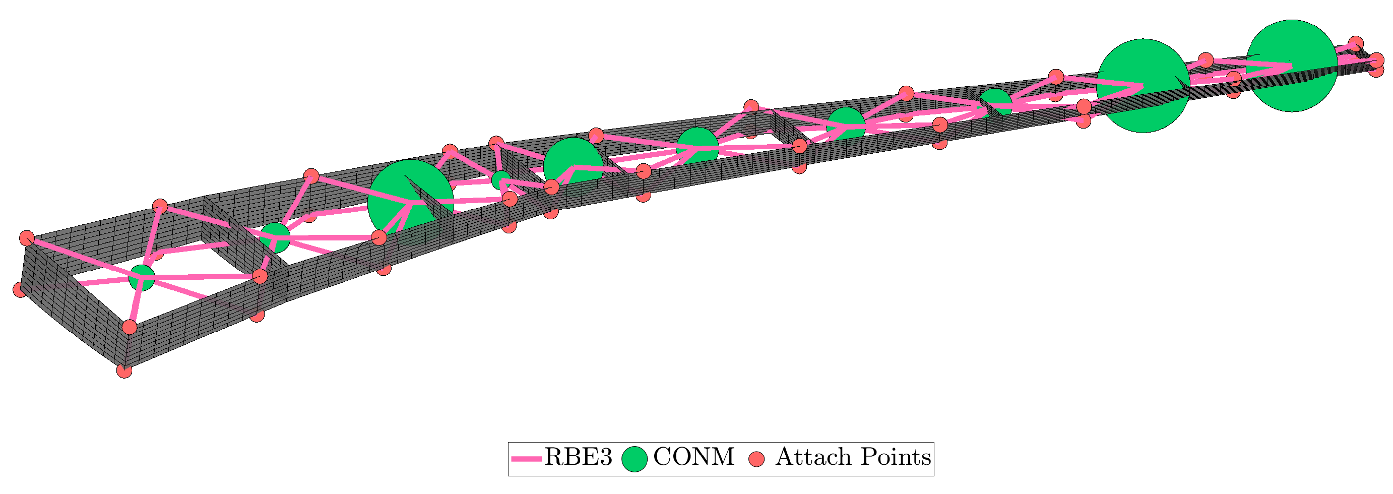
Figure 31.
Lumped masses for scaling.

Table 13.
Design variables of the optimization problem.
| Variable | Lower Bound | Upper Bound | Dimension |
|---|---|---|---|
| Ribs Number | 6 | 30 | 1 |
| Stringers Number | 4 | 10 | 1 |
| Front Spar Position | 0.1 | 0.4 | 1 |
| Rear Spar Position | 0.5 | 0.9 | 1 |
| Thicknesses at Control Points | 0.4 mm | 8 mm | 66 |
| Lumped Masses | 100 mg | 60 kg | 10 |
Total Design Variables .
At first, a single-step optimization run was performed with the modal objective accounting for the 10 first modes, and an accuracy level of 0.5 was set for the constraints handling. The modal objective couldn’t provide an acceptable level of matching as the Figure 32 depicts, but the constraints violation converged to an allowable level (Figure 33). In order to have an acceptable matching the modal objective should be lower than 0.2-0.3. Also, the feasible points found did not exhibit an in-flight shape that matched the target shape with acceptable accuracy.
The leading cause of the inability to converge to an acceptable value was the high elastic modulus of aluminium in combination with the reduced aerodynamic loads. The deformation of the scale wing was relatively low compared to the reference wing, and the thickness variables converged towards their lower limit. So a change was made in the material, and magnesium was chosen, whose properties are shown in the Table 14.
In order to reduce the computing time and converge to feasible solutions with acceptable accuracy, the optimization routine was modified to a serial optimization where the flight shape difference is first optimized. Then the modal response of the wing is also optimized while the optimized stiffness parameters are kept constant. A downside of this choice is that the resulting optimized parameters are potentially a sub-optimal of the scaling problem, as stated in [33].
4.2.6. Static Aeroelastic Response
Static aeroelastic similarity optimization was set and run twice with different FOCUS parameter values (Table 15). The tolerance for the violation of the Von Mises constraint was set to 2.
Figure 34 displays the evolution of the objective function with the number of iterations. In less than 500 iterations, the RMS error of the in-flight shape difference has converged to an optimal value of . After the first run, the focus parameter was set to 10, and the routine was recompiled and converged (Figure 35) to an optimal value of or .
The optimal thickness DVs are depicted in Figure 36 and the geometric DVs are presented in Table 16.
In Figure 37, we see the in-flight shape of the best-found point (with the specified tolerance) compared to the in-flight target shape scaled from the reference aircraft. The in-flight shape fits well overall along the wing except for the nodes near the wing tip. In fact, as Figure 38 represents, an inaccuracy is observed at the AoA of the sections near the wing-tip. A solution to this problem would be the consideration of wing tip torsion equality between the scaled and reference wing as a constraint.
Regarding the stress constraint, it is not active for the best-found point. As we can see in Figure 39, the maximum von Mises stress on the structure for the limit load condition is 149 MPa, compared to the defined allowable of 150 MPa.
4.2.7. Modal Response
The previously described mode similarity optimization problem was performed for the first N = 5 reference modes using the MIDACO optimizer. We can see the evolution of the objective function and constraints with the number of iterations, as shown in Figure 40 and Figure 41 respectively. The frequency constraints converge to the required value of 0, with a maximum relative error of 0.63 % for the scaled natural frequencies. The scaled total mass constraint converges with an error of 0.19 %.
The minimum of the objective function—characterizing the mode shape similarity that satisfies the constraints within the mentioned errors is , which implies that the average MAC value of the N = 5 modes considered for the comparison is . Therefore, the results indicate a good matching for the first 5 modes according to Girard and Roy’s guidelines. However, mode shapes 6–10 are dissimilar, and the improvement of the framework is necessary to fully match the modal response.
The mass DVs are presented in Figure 42 and their corresponding values are those presented in Table 17. Finally, The eigenfrequency of each mode is presented in Table 18. The average error of the eigenfrequencies is 14.44%.
Figure 43 shows the comparison of the reference modes and the ones of the best design found by MIDACO after 170 iterations.
An attempt for optimization of N=10 modes was also conducted. As seen in Figure 44 and Figure 45 the optimizer did not converge to a satisfying objective value and focused on the demanding constraint fulfilment. A multi-start optimization technique would give us a more correct view of the convergence ability of the problem.
As a result, it would be better to focus on the exact matching of a more limited number of modes, instead of trying to match relatively large numbers of modes (e.g., N = 10) and obtain a lower average result.
4.2.8. Flutter Speed
The results are depicted in Figure 46. Since flutter is defined as the point where the oscillations (naturally damped before the flutter speed) start to diverge, the flutter point is identified when the damping plotted against the airspeed turns from negative to positive values. In the Figure 46 we obtain that the first mode turns from negative to positive at around .
4.2.9. Effectiveness of Geometrical Parameterization
The main novelty of this study is the introduction of geometric parameters in the optimization framework. The number of ribs is a parameter that has a significant role in stiffness and mass distribution. It affects the spanwise torsional stiffness of the wing and, thus, is a parameter that controls the wing’s torsion, which has a significant role in static and dynamic aeroelastic phenomena. Moreover, the spars’ position is an essential tool for the control of the bending stiffness of the wing. Adjusting the spars’ position affects the moment of inertia in the X and Z direction (because of the airfoil’s thickness distribution) and consequently the displacements in the Z and X directions, thus achieving a better matching between the two wings. Consequently, by adjusting those three variables, we can effectively affect the torsional stiffness, bending stiffness and mass distribution.
In Figure 47 and Figure 48 the convergence of those variables is demonstrated. It is obvious that the algorithm tried to adjust the parameters appropriately so that there is a substantial reduction in torsional and bending stiffness in order to achieve greater similarity. The aerodynamic loads of the sub-scale model were noticeably lower, so reducing the number of ribs and placing the spars towards the trailing and leading edges reduced stiffness considerably. These parameters played a decisive role while the thickness parameters adjusted the spanwise stiffness distribution to achieve a similar deformation pattern.
5. Conclusions
This research study consists of the development of an aeroelastic optimization framework which with appropriate configuration is useful for either mass or similarity optimization between a sub-scale model and a reference wing. The core of the framework consists of the aeroelastic analysis (static and dynamic) combined with the appropriate functions for the objectives and constraints and an ACO algorithm (MIDACO). The parameterization of the wing includes geometric parameters and thicknesses for the stiffness distribution and 10 lumped masses for the mass distribution (for the scaling problem).
A mass optimization problem was initially set up for the uCRM wing. In this case, there were only geometric and thickness parameters (e.g., spar positions, number of ribs, number of stringers and thicknesses at specified control points). Stiffness, stress, and flutter constraints were included with target values being set based on the literature and the Civil Aviation Regulations FAR-25. The optimizer converged at a structural mass of while all the constraints were satisfied. Of interest are the optimized variables’ values. The thickness parameters decrease gradually along the wing, except of the Yehudi break where maximum stress usually arises. The spars’ position, as expected, converged around the position of the airfoil’s maximum thickness in order to optimize the stiffness in the x direction while the underestimated drag (because of the potential flow implemented by DLM does not require so much stiffness in the z direction. Finally, the ribs’ number converged to 51, which is close to the optimal solution presented in [37].
As far as the scaling problem is concerned, the objectives and constraints were modified in order to meet similarity requirements. In fact the problem’s objectives were the RMS error of in-flight shape difference and the average MAC of the N modes that were selected to optimize. The constraints included were the equality of each eigenfrequency, the equality of the model’s mass to a target value defined by the scaling parameters, and the avoidance of maximum stresses greater than the maximum allowable. Also, a constraint to avoid flutter at a certain speed for the optimal solution was considered.
The pre-described optimization problem was first run with a single-step approach, for N=10 modes to optimize and the material was aluminium. The results were deemed unacceptable. The RMS error of the in-flight shape difference converged to the value of 0.45, indicating bad matching of the static aeroelastic response. The constraints of the modal response were satisfied but the modal similarity was quite low indicating no similarity at all. These problems were addressed by changing the material to magnesium, changing the modes to match to N=5 and the one-step approach to a two-step (serial) approach in order to reduce the computing time and get acceptable results quicker. After those alterations, the optimizer converged to acceptable values indicating a good matching of both the static aeroelastic and modal response. In fact the RMS error of the in-flight shape difference of the optimal solution is and the mean MAC value of the first 5 modes is . The constraints of the problem were also satisfied but there is room for improvement mainly in terms of frequency error. As far as the flutter is concerned, the flutter speed of the optimal solution is way beyond the diving speed, indicating no flutter.
Of interest is the location of the spars, which are quite close to the leading and trailing edges, in contrast to the reference wing. This is likely due to the increased stiffness presented by the sub-scale structure given the reduced aerodynamic loads. Placing the spars towards the edges, reduces the stiffness around the x-axis and thus the structure becomes more flexible thus avoiding the very low values of the thicknesses and thus the construction difficulties. The number of ribs was also reduced to 15 in order to reduce the torsional stiffness of the wing indicating the significance of the parameterization of ribs’ number. Future implementations in the framework are directed towards the following:
- The investigation of other types of materials (such as wood or composites) and combination of them would greatly increase the design space and ensure the presence (or absence) of the effects of the full model (such as skin buckling).
- The calculation of derivatives in order to include a gradient-based optimizer in the framework. It will give the opportunity for a more efficient optimization since we take advantage of a gradient-free optimizer.
- Introduction of a high fidelity aerodynamic solver such as Euler or RANS. As already mentioned, the potential theory upon which the DLM is based, underestimates the drag distribution while overestimating the lift. A high-fidelity solver will avoid such problems and provide more accurate load prediction.
- The parameterization of the number of spars will give the opportunity to design wings with more than two spars and it will greatly increase the design space. Also, it will allow the design of other types of wings such as military aircraft wings that incorporate multi-spar configurations.
Author Contributions
Conceptualization, A.K., S.K., E.F. and V.K.; methodology, E.F. and S.K.; software, E.F.; validation, E.F.; formal analysis, E.F.; investigation, E.F. and S.K.; resources, E.F. and S.K.; data curation, E.F.; writing—original draft preparation, E.F. and S.K.; writing—review and editing, E.F., S.K., A.K. and V.K.; visualization, E.F.; supervision, A.K., S.K. and V.K.; project administration, A.K. and V.K.;. All authors have read and agreed to the published version of the manuscript.
Funding
The authors gratefully acknowledge the financial support of EU, H2020 CS2 project under the acronym GRETEL (Grant agreement ID: 737671).

Institutional Review Board Statement
Not applicable.
Informed Consent Statement
Not applicable.
Data Availability Statement
Data are available upon request.
Conflicts of Interest
The authors declare no conflict of interest.
Abbreviations
The following abbreviations are used in this manuscript:
| ACO | Ant Colony optimization |
| AoA | Angle of Attack |
| AR | Aspect Ratio |
| CAE | Computational Aided Engineering |
| CFD | Computational Fluid Dynamics |
| CSM | Computational Structural Mechanics |
| DV | Design Variables |
| FEM | Finite Element Method |
| FSI | Fluid-Structure Interaction |
| DLM | Doublet Lattice Method |
| LES | Large Eddy Simulation |
| MAC | Modal Assurance Criterion |
| MDO | Multidisciplinary Design Optimization |
| NS | Navier-Stokes |
| OML | Outer Mold Line |
| RANS | Reynolds Averaged Navier Stokes |
| RMS | Root Mean Square |
| VLM | Vortex Lattice Method |
| uCRM | undeflected Common Research Model |
References
- Andersen, G.; Cowan, D.; Piatak, D. Aeroelastic Modeling, Analysis and Testing of a Morphing Wing Structure. 48th AIAA/ASME/ASCE/AHS/ASC Structures, Structural Dynamics, and Materials Conference; American Institute of Aeronautics and Astronautics: Honolulu, Hawaii, 2007. [CrossRef]
- The European Commission. Reducing emissions from aviation; The European Commission, 2021.
- Anderson, J.D. Fundamentals of aerodynamics, 6th ed.; McGraw-Hill series in aeronautical and aerospace engineering; McGraw Hill Education: New York, NY, USA, 2017. [Google Scholar]
- Castellani, M.; Cooper, J.E.; Lemmens, Y. Nonlinear Static Aeroelasticity of High-Aspect-Ratio-Wing Aircraft by Finite Element and Multibody Methods. Journal of Aircraft 2017, 54, 548–560. [Google Scholar] [CrossRef]
- Garrigues, E. A Review of Industrial Aeroelasticity Practices at Dassault Aviation for Military Aircraft and Business Jets. AerospaceLab Journal 2018, Issue 14, 34 pages. Artwork Size: 34 pages Medium: PDF Publisher: ONERA. [CrossRef]
- Afonso, F.; Vale, J.; Oliveira, É.; Lau, F.; Suleman, A. A review on non-linear aeroelasticity of high aspect-ratio wings. Progress in Aerospace Sciences 2017, 89, 40–57. [Google Scholar] [CrossRef]
- Katz and, J.; Plotkin, A. Low-Speed Aerodynamics, Second Edition. Journal of Fluids Engineering 2004, 126, 293–294. [Google Scholar] [CrossRef]
- Murua, J.; Palacios, R.; Graham, J.M.R. Applications of the unsteady vortex-lattice method in aircraft aeroelasticity and flight dynamics. Progress in Aerospace Sciences 2012, 55, 46–72. [Google Scholar] [CrossRef]
- Schmit, L.A. Structural design by systematic synthesis. Proceedings of the Second National Conference on Electronic Computation, ASCE, Sept., 1960, 1960.
- Shirk, M.H.; Hertz, T.J.; Weisshaar, T.A. Aeroelastic tailoring-theory, practice, and promise. Journal of Aircraft 1986, 23, 6–18. [Google Scholar] [CrossRef]
- Shuart, M.J.; Haftka, R.T.; Campbell, R. Optimum design of swept-forward high-aspect-ration graphite-epoxy wings. Recent Advances in Multidisciplinary Analysis and Optimization, Part 1 1989.
- Martins, J.R.R.A.; Ning, A. Engineering Design Optimization; Cambridge University Press, 2021. [CrossRef]
- De, S. Structural Modeling and Optimization of Aircraft Wings having Curvilinear Spars and Ribs (SpaRibs); 2017.
- Stodieck, O.; Cooper, J.E.; Weaver, P.M.; Kealy, P. Aeroelastic Tailoring of a Representative Wing Box Using Tow-Steered Composites. AIAA Journal 2017, 55, 1425–1439. [Google Scholar] [CrossRef]
- Gray, A.C.; Martins, J.R. Geometrically Nonlinear High-fidelity Aerostructural Optimization for Highly Flexible Wings. AIAA Scitech 2021 Forum, 2021, p. 0283. [CrossRef]
- Sinha, K.; Klimmek, T.; Schulze, M.; Handojo, V. Loads analysis and structural optimization of a high aspect ratio, composite wing aircraft. CEAS Aeronaut J 2021, 12, 233–243. [Google Scholar] [CrossRef]
- Li, W.W.; Pak, C.g. Aeroelastic Optimization Study Based on the X-56A Model. AIAA Atmospheric Flight Mechanics Conference; American Institute of Aeronautics and Astronautics: Atlanta, GA, 2014. [CrossRef]
- Dillinger, J. Static aeroelastic optimization of composite wings with variable stiffness laminates. PhD thesis, Delft University of Technology, 2014.
- Regier, A.A. Vibration-Response Tests of a 1/5-Scale Model of the Grumman F6F Airplane in the Langley 16-Foot High-Speed Tunnel. Technical report, 1944.
- Kuzmina, S.I.; Ishmuratov, F.; Zichenkov, M.; Chedrik, V. Integrated numerical and experimental investigations of the Active/Passive Aeroelastic concepts on the European Research Aeroelastic Model (EuRAM). Journal of Aeroelasticity and Structural Dynamics 2011, 2. [Google Scholar]
- Chen, P.; Ritz, E.; Lindsley, N. Nonlinear flutter analysis for the scaled F-35 with horizontal-tail free play. Journal of aircraft 2014, 51, 883–889. [Google Scholar] [CrossRef]
- Stanford, B. Scaled Aeroelastic Wind Tunnel Model Design with Topology Optimization. AIAA AVIATION 2021 FORUM, 2021, p. 3083. [CrossRef]
- French, M. An application of structural optimization in wind tunnel model design. 31st Structures, Structural Dynamics and Materials Conference, 1990, p. 956.
- French, M.; Eastep, F. Aeroelastic model design using parameter identification. Journal of aircraft 1996, 33, 198–202. [Google Scholar] [CrossRef]
- Richards, J.; Suleman, A.; Canfield, R.; Blair, M. Design of a scaled RPV for investigation of gust response of joined-wing sensorcraft. 50th AIAA/ASME/ASCE/AHS/ASC Structures, Structural Dynamics, and Materials Conference 17th AIAA/ASME/AHS Adaptive Structures Conference 11th AIAA No, 2009, p. 2218.
- Ricciardi, A.P.; Eger, C.A.; Canfield, R.A.; Patil, M.J. Nonlinear aeroelastic-scaled-model optimization using equivalent static loads. Journal of Aircraft 2014, 51, 1842–1851. [Google Scholar] [CrossRef]
- Wan, Z.; Cesnik, C.E. Geometrically nonlinear aeroelastic scaling for very flexible aircraft. AIAA Journal 2014, 52, 2251–2260. [Google Scholar] [CrossRef]
- Ricciardi, A.P.; Canfield, R.A.; Patil, M.J.; Lindsley, N. Nonlinear Aeroelastic Scaled-Model Design. Journal of Aircraft 2016, 53, 20–32. [Google Scholar] [CrossRef]
- Pontillo, A.; Hayes, D.; Dussart, G.X.; Lopez Matos, G.E.; Carrizales, M.A.; Yusuf, S.Y.; Lone, M.M. Flexible high aspect ratio wing: low cost experimental model and computational framework. 2018 AIAA Atmospheric Flight Mechanics Conference, 2018, p. 1014.
- Spada, C.; Afonso, F.; Lau, F.; Suleman, A. Nonlinear aeroelastic scaling of high aspect-ratio wings. Aerospace Science and Technology 2017, 63, 363–371. [Google Scholar] [CrossRef]
- Mas Colomer, J.; Bartoli, N.; Lefebvre, T.; Martins, J.R.; Morlier, J. An MDO-based methodology for static aeroelastic scaling of wings under non-similar flow. Structural and Multidisciplinary Optimization 2021, 63, 1045–1061. [Google Scholar] [CrossRef]
- Venkataraman, S.; Haftka, R.T. Structural optimization complexity: what has Moore’s law done for us? Structural and Multidisciplinary Optimization 2004, 28, 375–387. [Google Scholar] [CrossRef]
- Mas Colomer, J.; Bartoli, N.; Lefebvre, T.; Dubreuil, S.; Martins, J.R.R.A.; Benard, E.; Morlier, J. Similarity Maximization of a Scaled Aeroelastic Flight Demonstrator via Multidisciplinary Optimization. 58th AIAA/ASCE/AHS/ASC Structures, Structural Dynamics, and Materials Conference; American Institute of Aeronautics and Astronautics: Grapevine, Texas, 2017. [CrossRef]
- Albano, E.; Rodden, W.P. A doublet-lattice method for calculating lift distributions on oscillating surfaces in subsonic flows. AIAA journal 1969, 7, 279–285. [Google Scholar] [CrossRef]
- Nastran, M. Aeroelastic Analysis User’s Guide. MSC Software Corporation 2004.
- Schlüter, M.; Egea, J.A.; Banga, J.R. Extended ant colony optimization for non-convex mixed integer nonlinear programming. Computers & Operations Research 2009, 36, 2217–2229. [Google Scholar] [CrossRef]
- Brooks, T.R.; Kenway, G.K.W.; Martins, J.R.R.A. Benchmark Aerostructural Models for the Study of Transonic Aircraft Wings. AIAA Journal 2018, 56, 2840–2855. [Google Scholar] [CrossRef]
- Martins, J.R.; Kenway, G.K.; Burdette, D.; Jonsson, E.; Kennedy, G.J. High-Fidelity Multidisciplinary Design Optimization of Aircraft Configurations. Technical report, 2017.
- Dababneh, O.; Kipouros, T.; Whidborne, J.F. Application of an efficient gradient-based optimization strategy for aircraft wing structures. Aerospace 2018, 5, 3. [Google Scholar] [CrossRef]
- Liu, Q.; Mulani, S.B.; Kapania, R.K. Global/local multidisciplinary design optimization of subsonic wing. 10th AIAA Multidisciplinary Design Optimization Conference, 2014, p. 0471.
- Wikipedia contributors. List of wind tunnels — Wikipedia, The Free Encyclopedia, 2022. [Online; accessed 25-September-2022].
- Pires, T. Linear Aeroelastic Scaling of a Joined Wing Aircraft. Instituto Superior Tecnico, TU Lisbon 2014.
- Girard, A.; Roy, N. Structural dynamics in industry; Vol. 7, John Wiley & Sons, 2010. [CrossRef]
| 1 | More information about uCRM wing can be found in: https://commonresearchmodel.larc.nasa.gov/. |
Figure 1.
Commercial aircraft wings aspect ratio trend [4].
Figure 1.
Commercial aircraft wings aspect ratio trend [4].
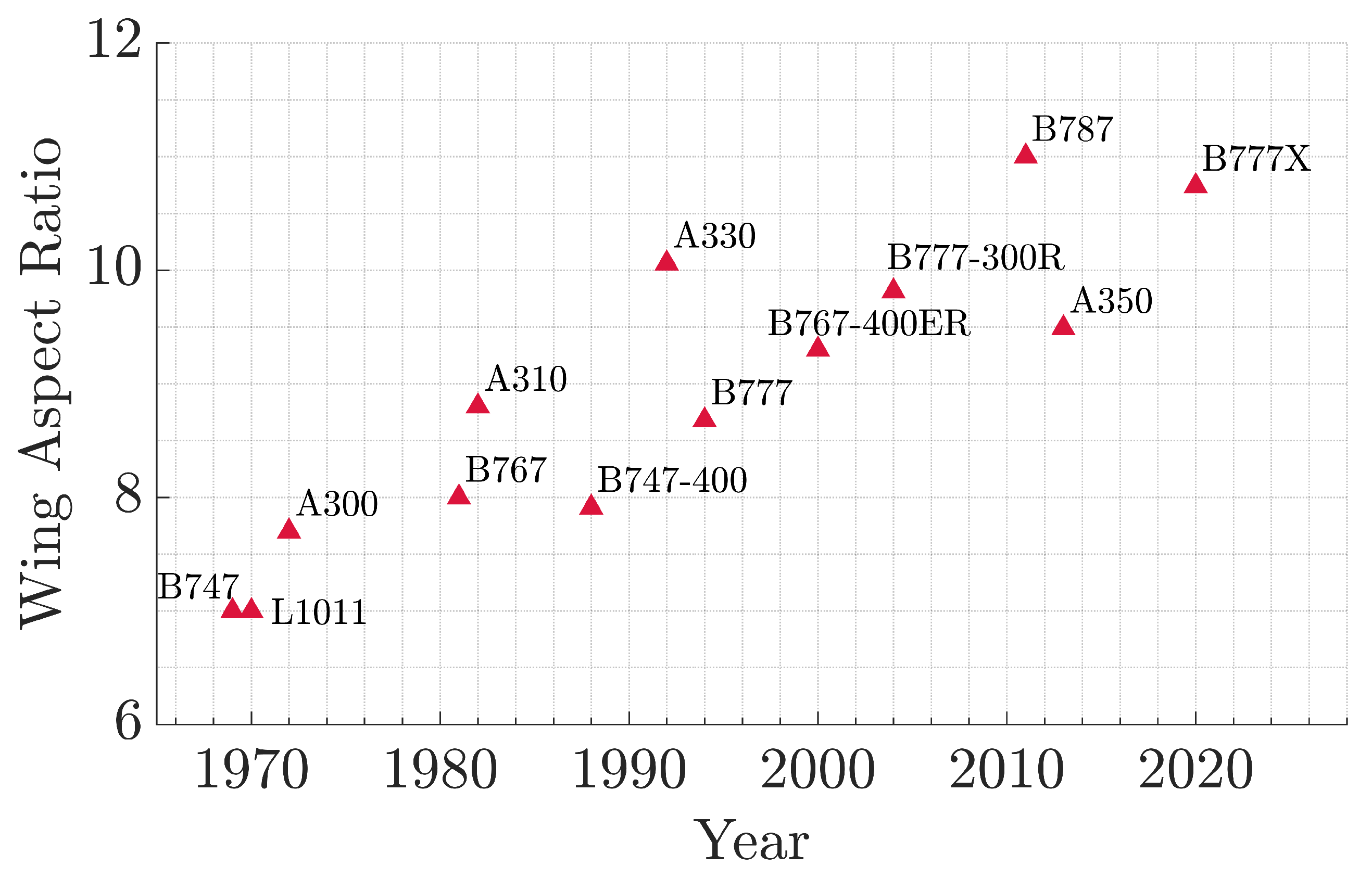
Figure 2.
Modern approach for aeroelastic effects investigation.
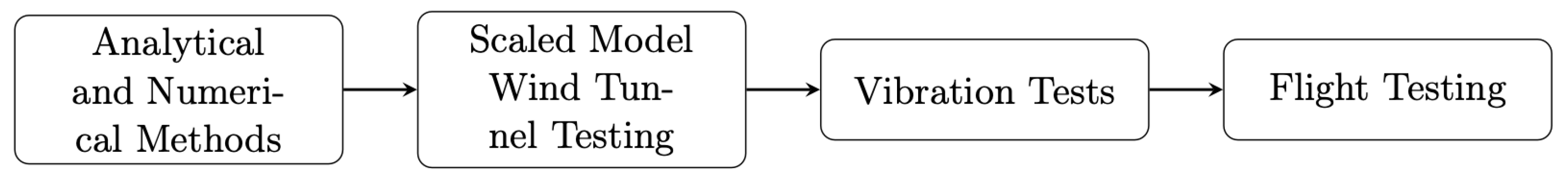
Figure 3.
Aerodynamic models used in aeroelastic calculations.
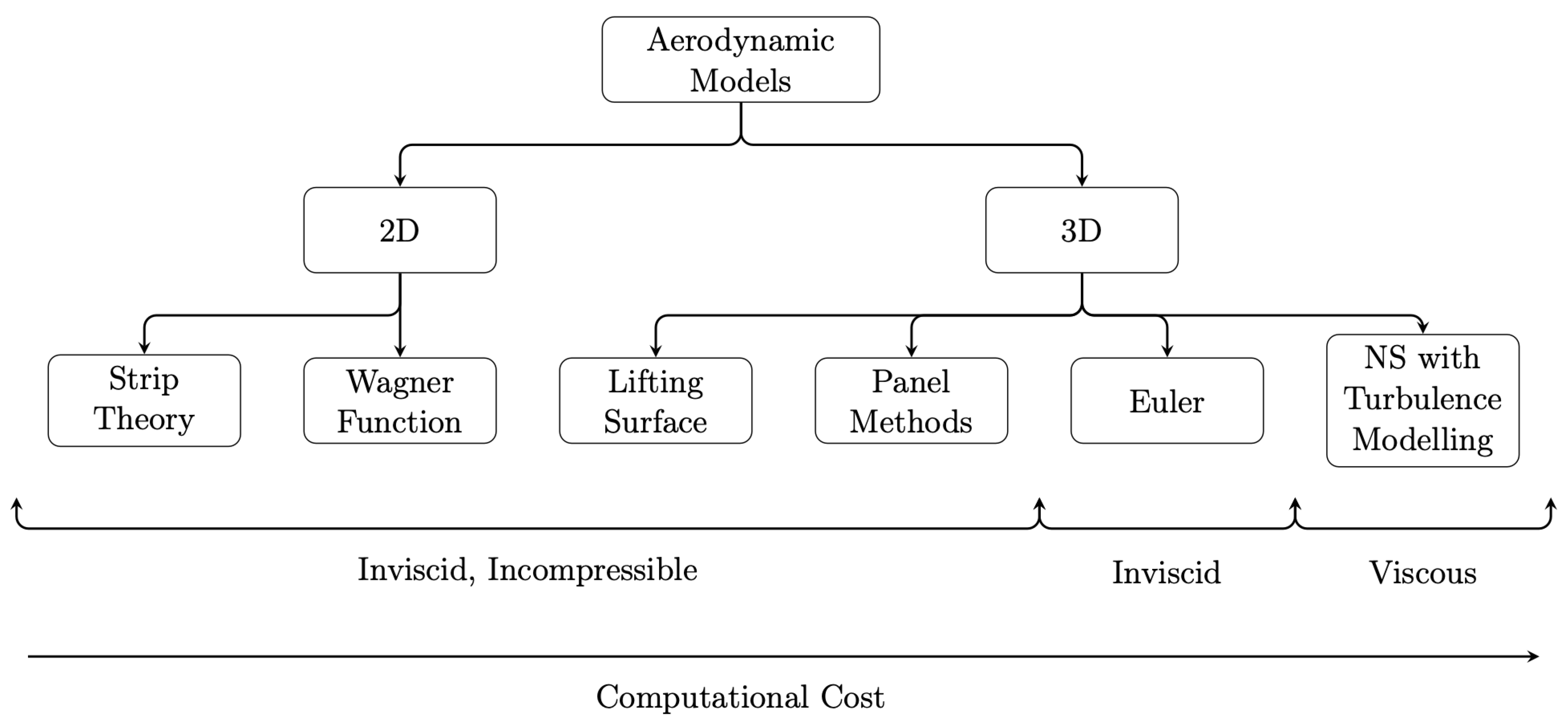
Figure 4.
Structural models used in aeroelastic calculations.
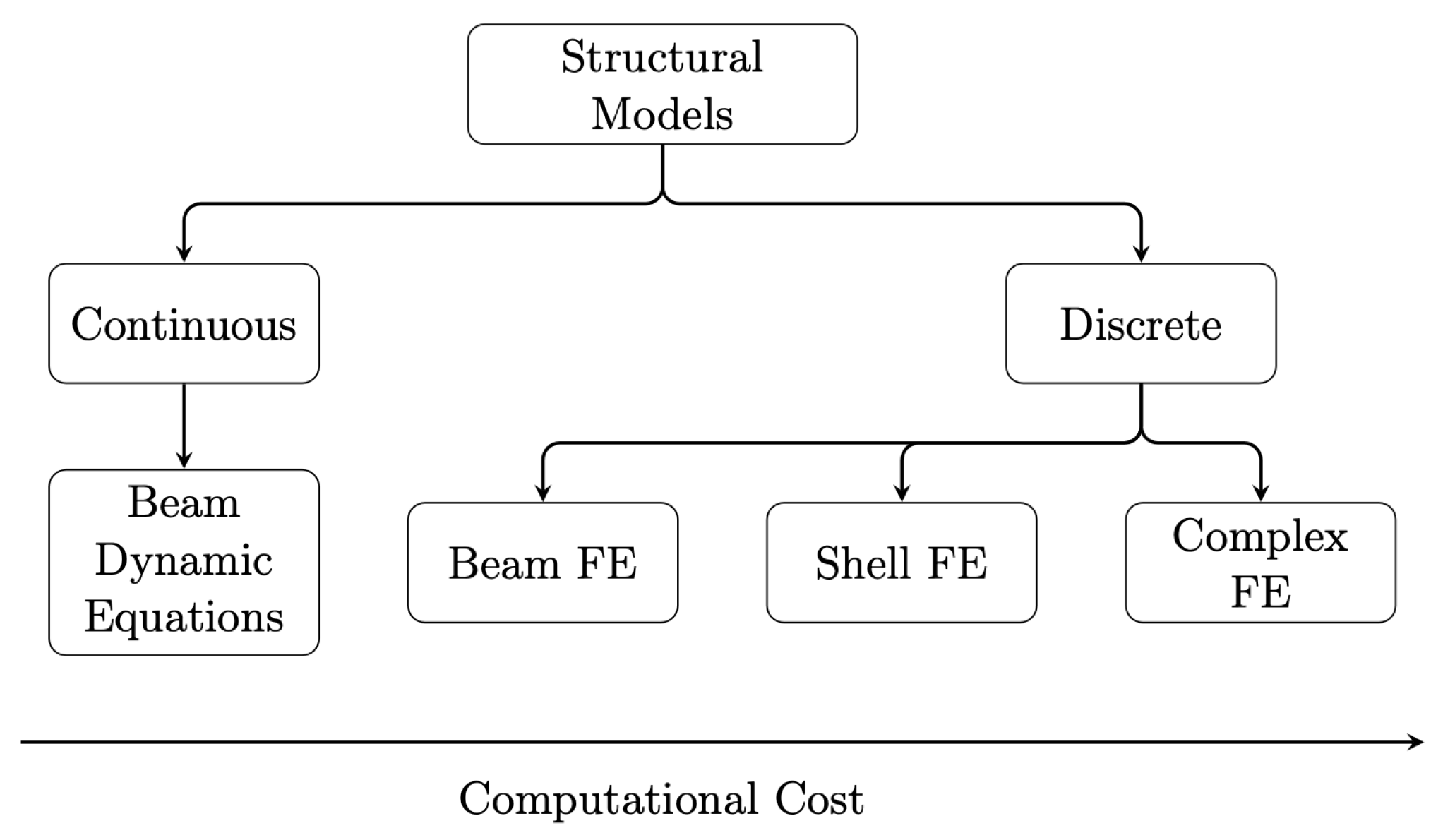
Figure 5.
The American experimental aircraft Grumman X-29.
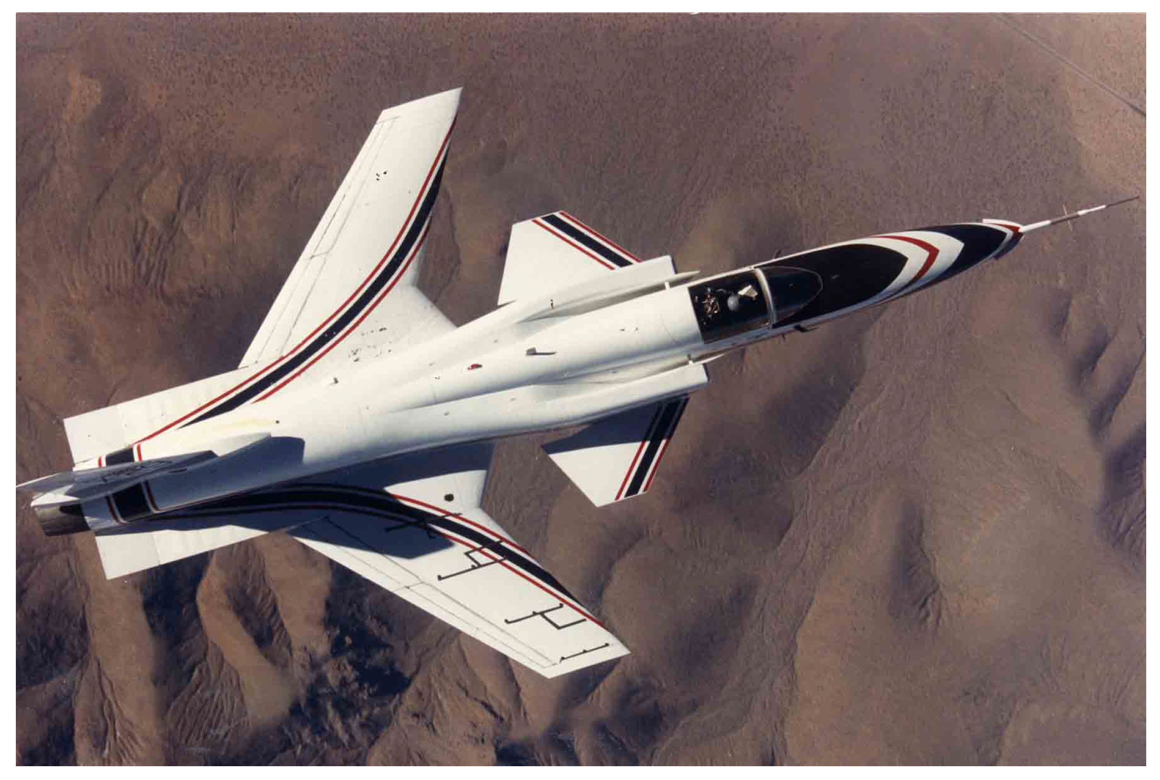
Figure 6.
High subsonic flutter model of Grumman F6F in NACA Langley Memorial Aeronautical Laboratory [19].
Figure 6.
High subsonic flutter model of Grumman F6F in NACA Langley Memorial Aeronautical Laboratory [19].
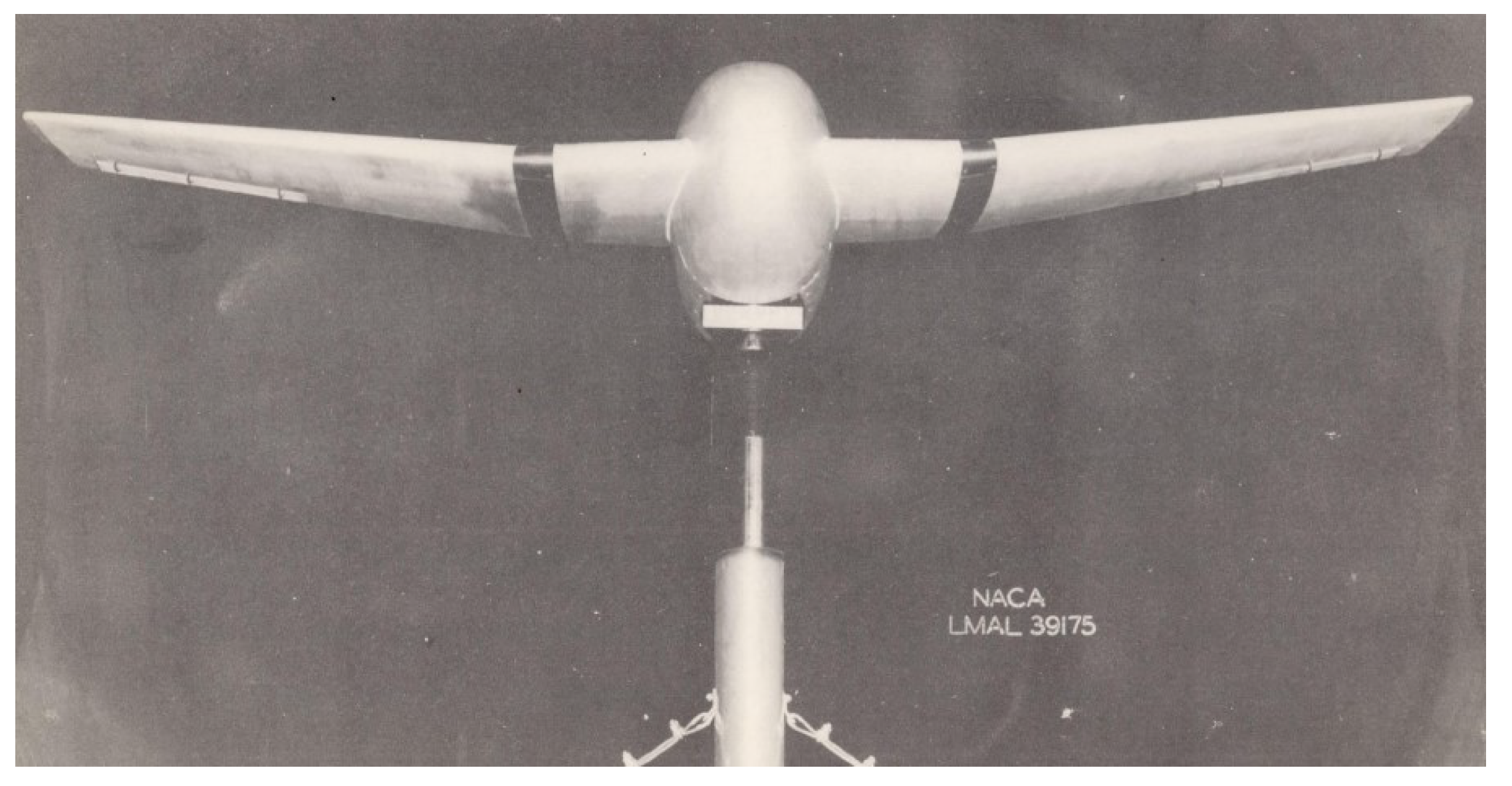
Figure 7.
Recent aeroelastic scaling practises ([20,21,22]).
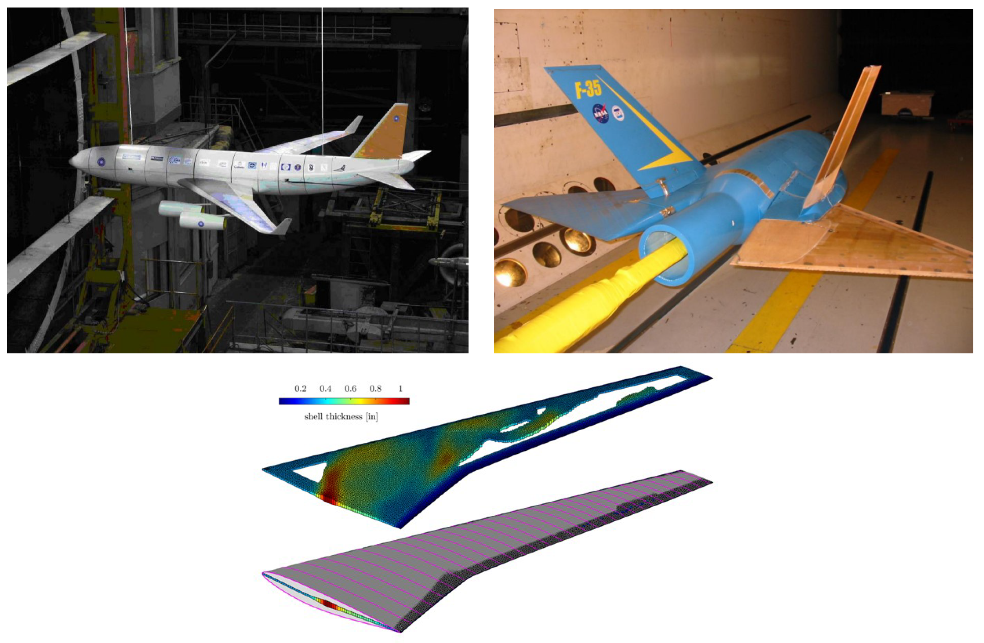
Figure 8.
Example of FEM mesh with shell and beam elements.
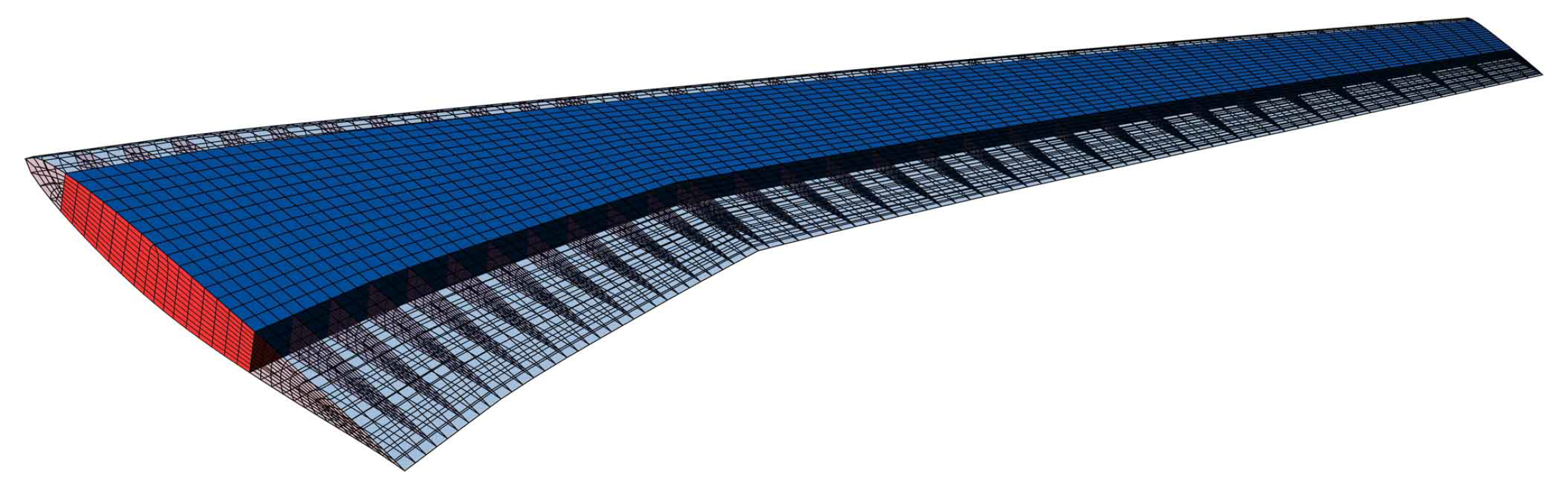
Figure 9.
3D wing surface modeled by flat panels.
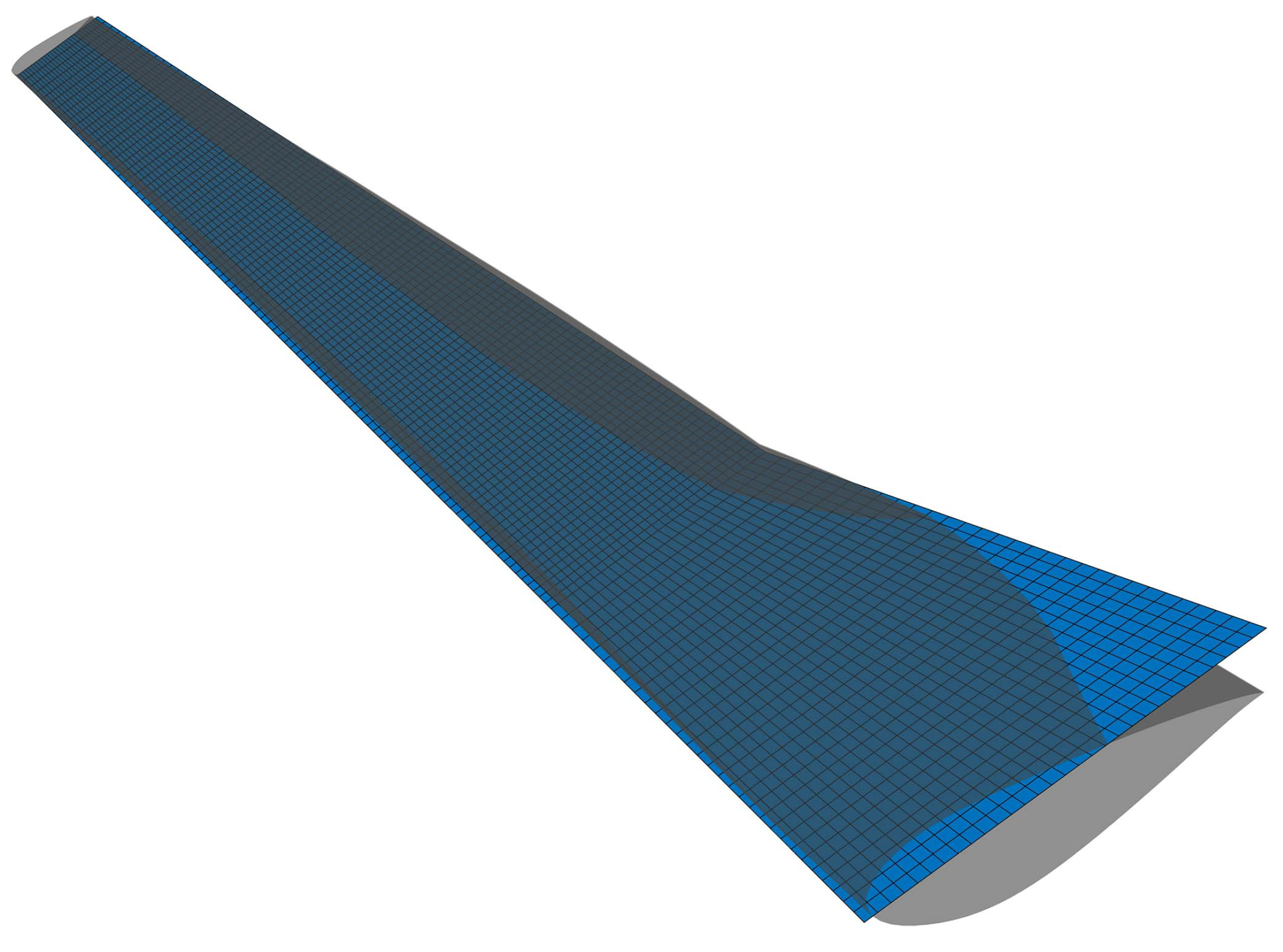
Figure 10.
Mean camber line construction method.
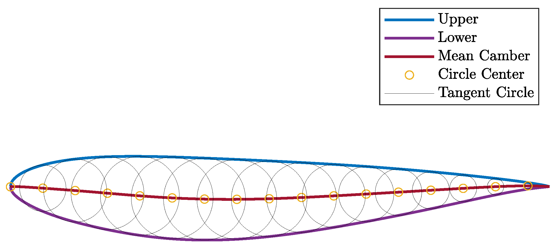
Figure 11.
W2GJ matrix influence on boxes’ inclination.
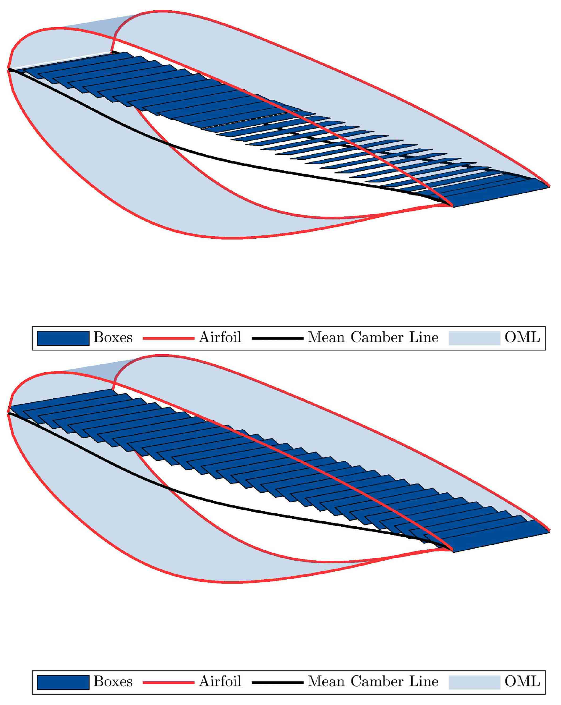
Figure 12.
Example of coupling nodes in a wing.
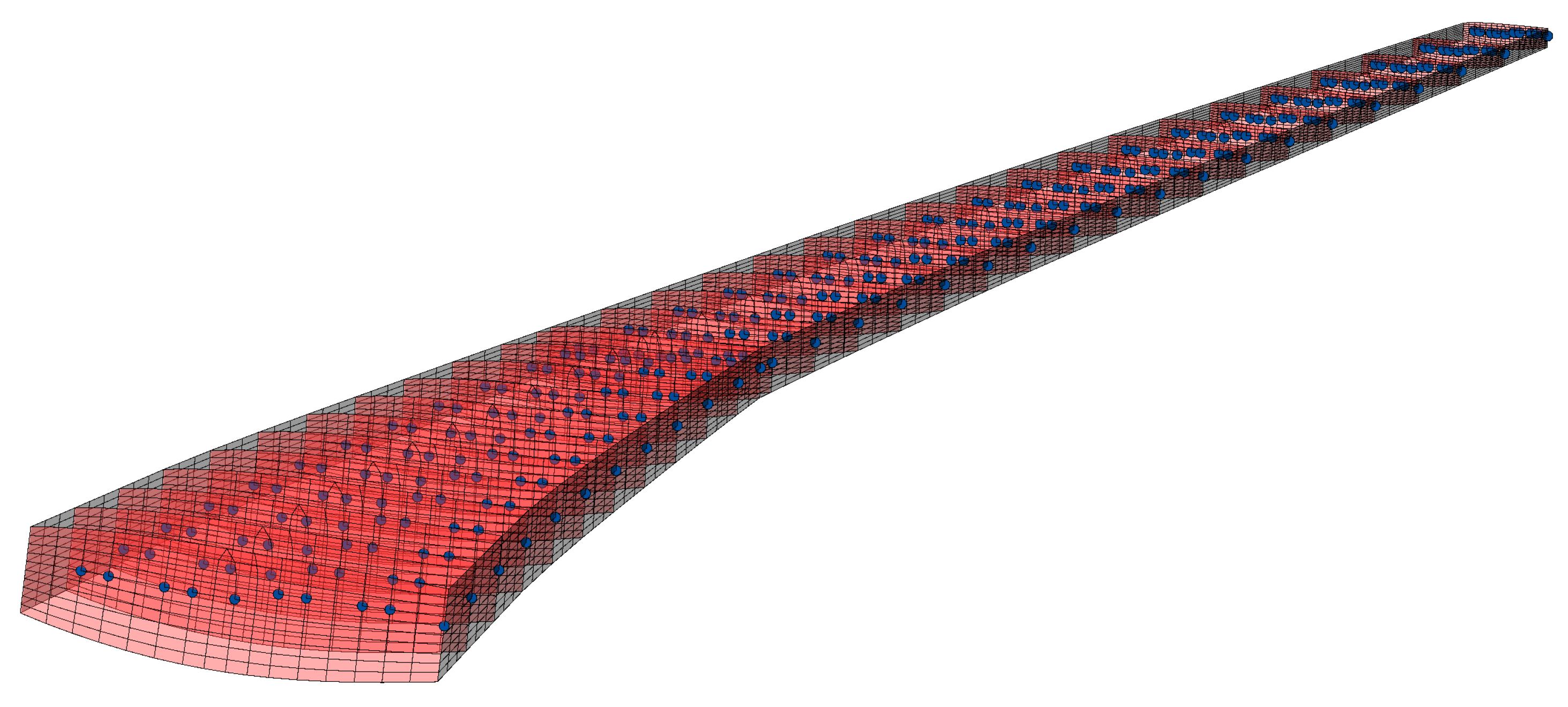
Figure 13.
Static aeroelastic framework flowchart.
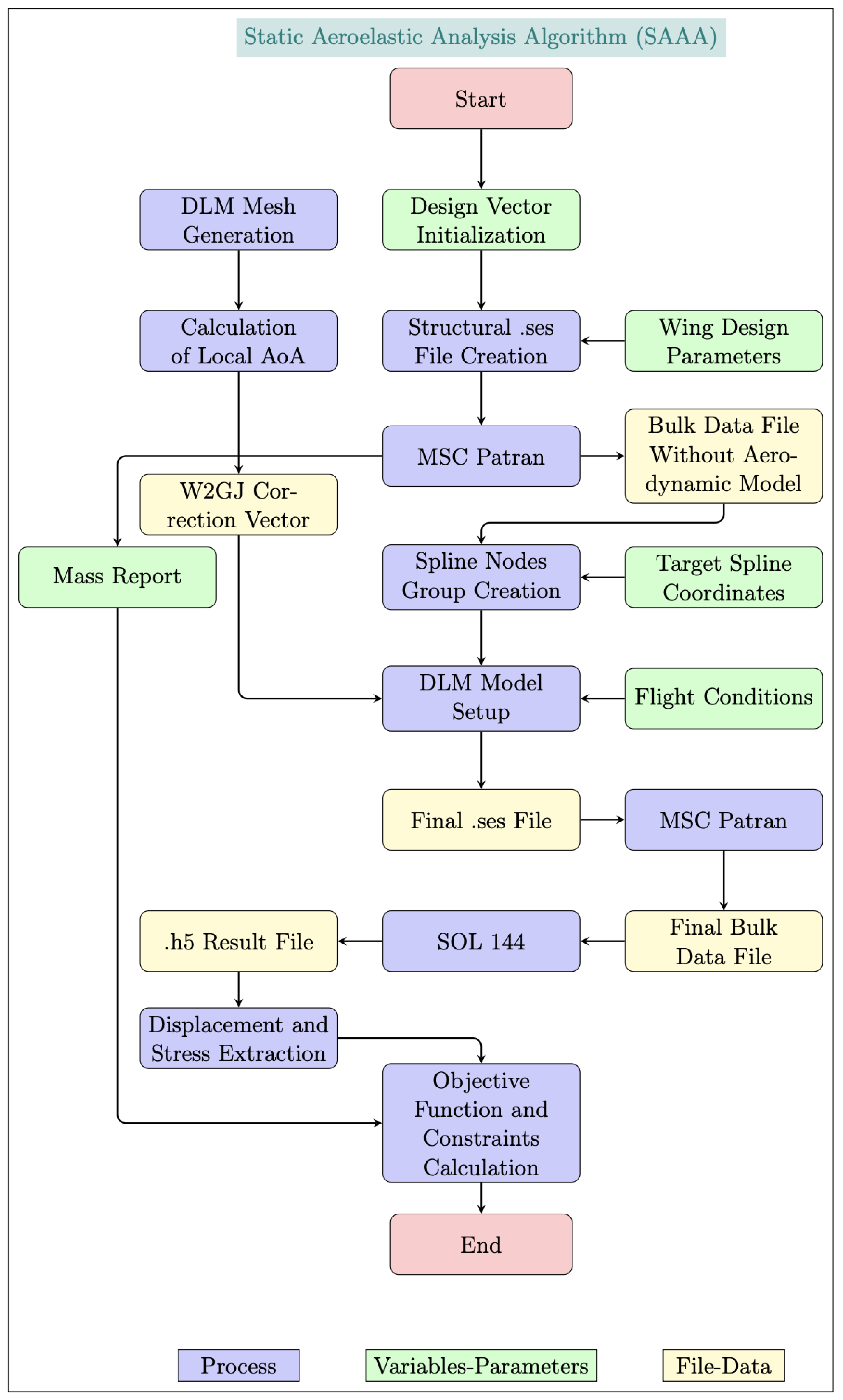
Figure 14.
Modal analysis framework flowchart.
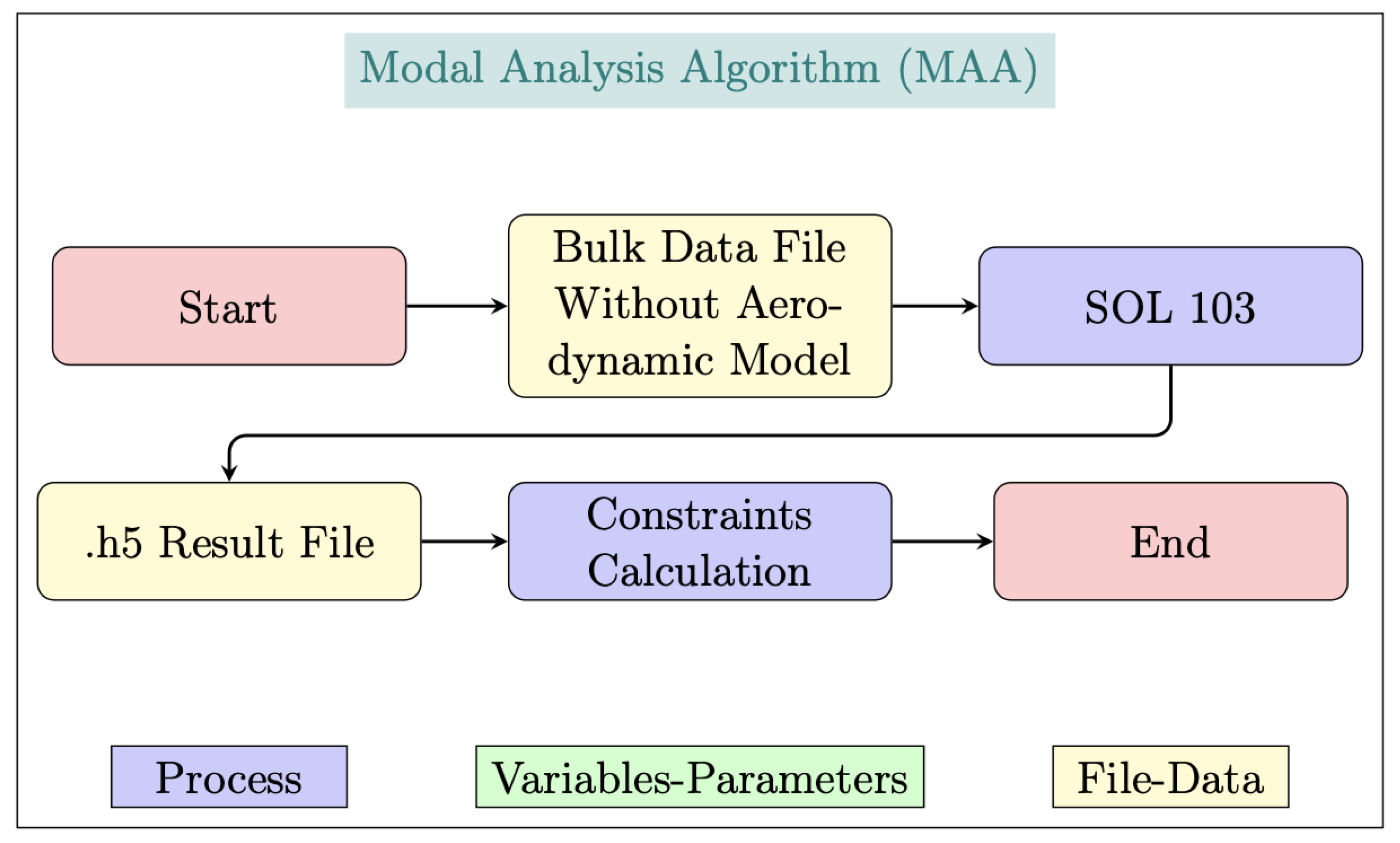
Figure 15.
Dynamic aeroelastic framework flowchart.
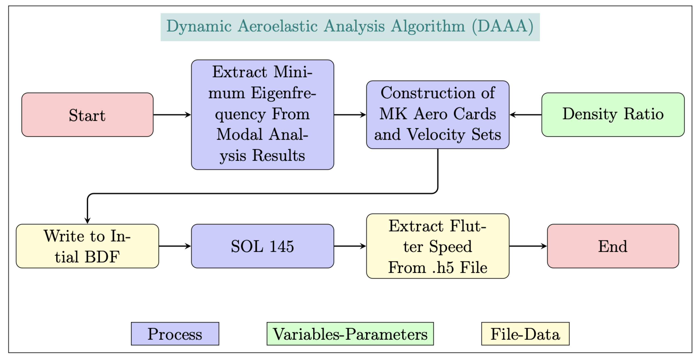
Figure 16.
Aeroelastic optimization framework flowchart.
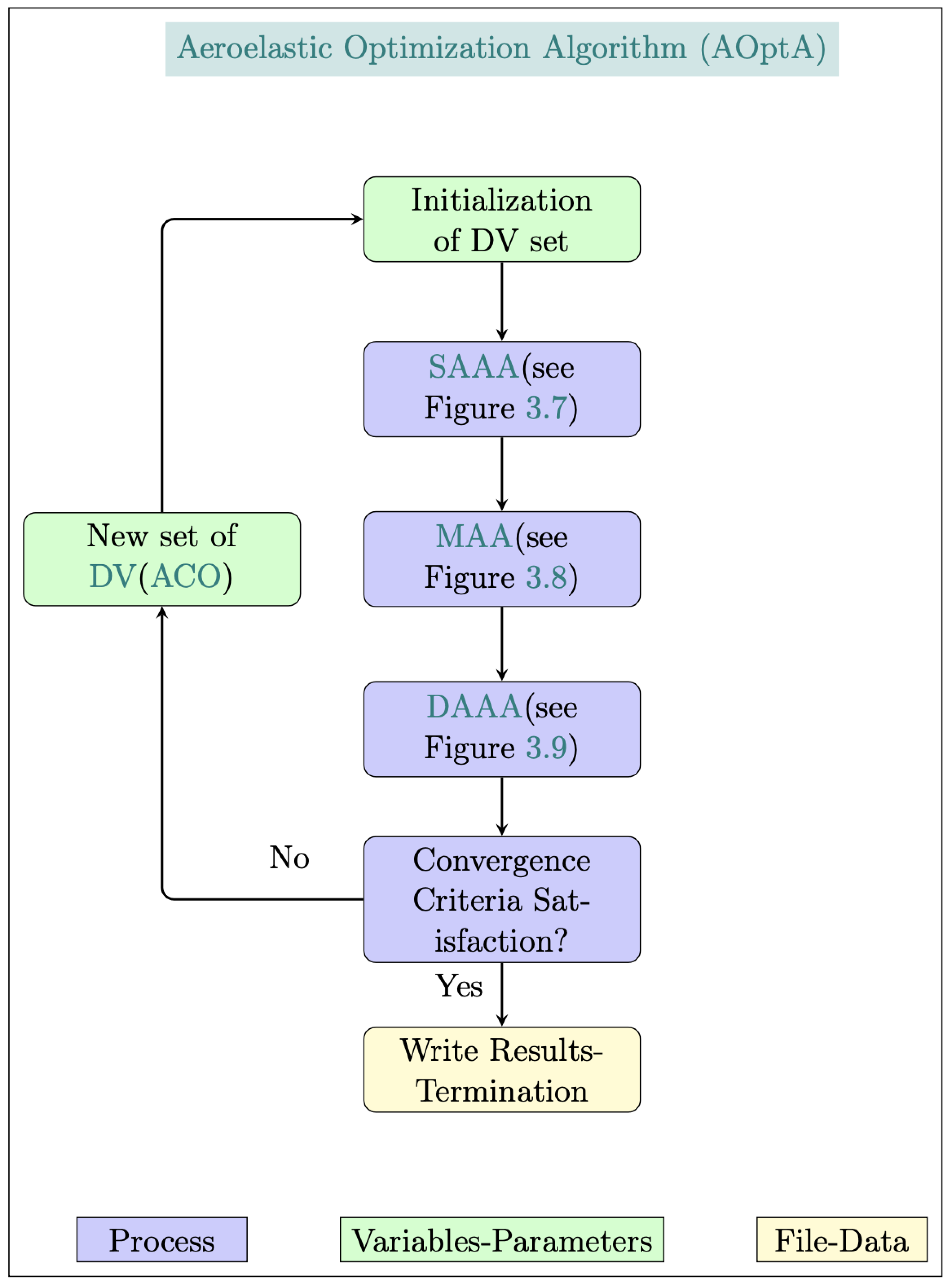
Figure 17.
Aeroelastic scaling framework flowchart.
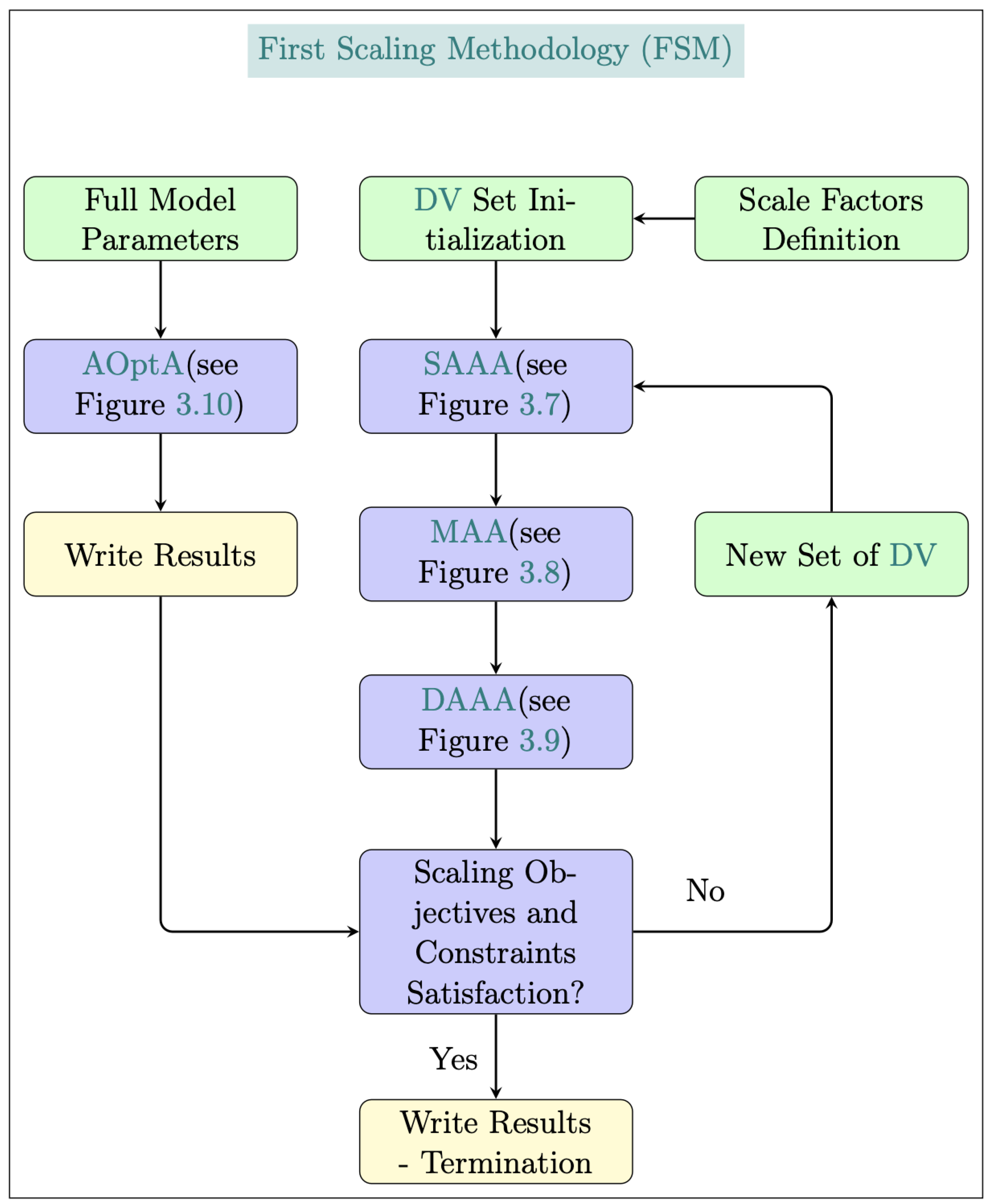
Figure 18.
uCRM wing OML and internal structure.
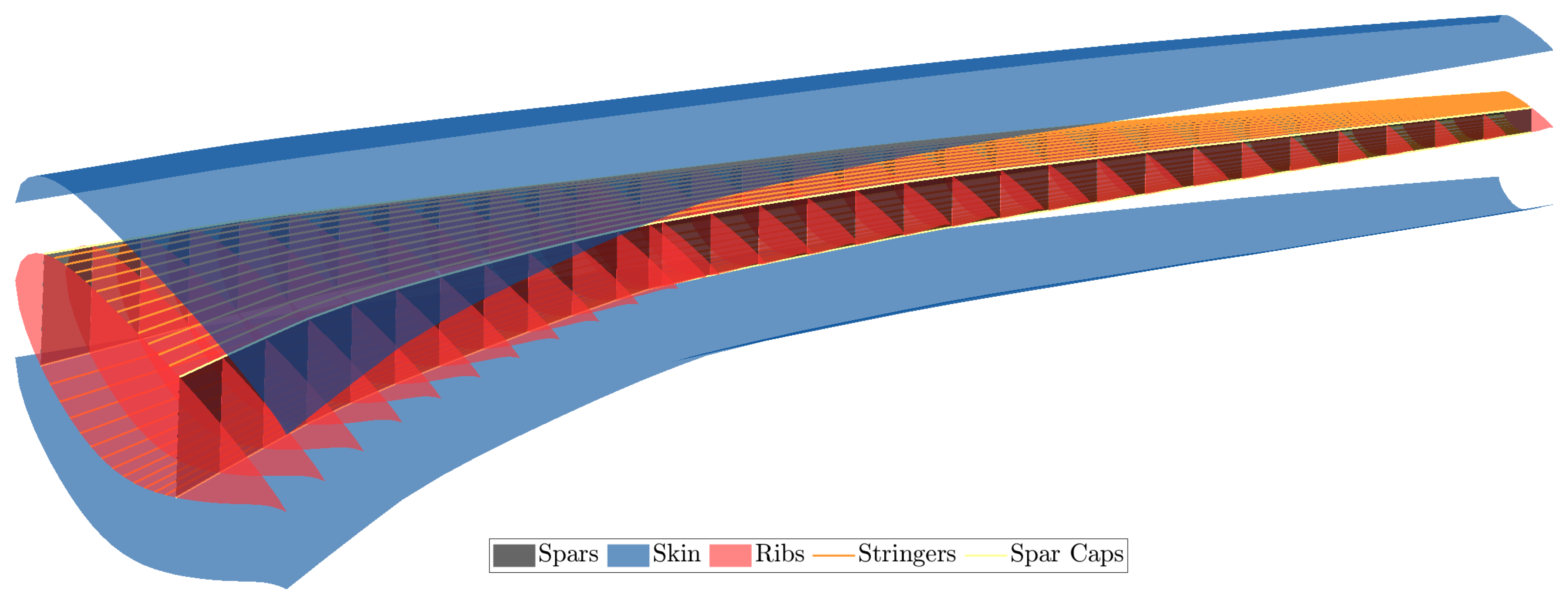
Figure 19.
uCRM wing twist distribution.
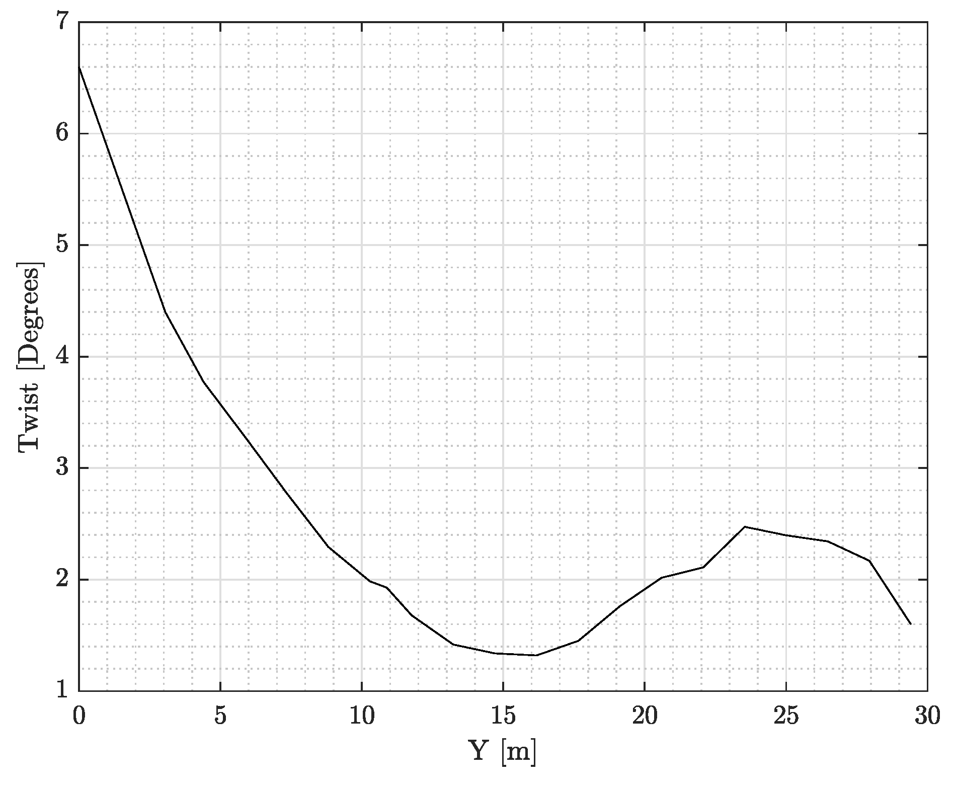
Figure 20.
Objective and constraints violation during the 1st run.
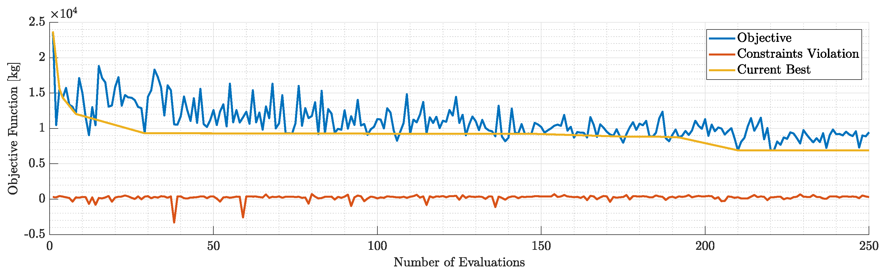
Figure 21.
Violation of each constraint during the 1st run.
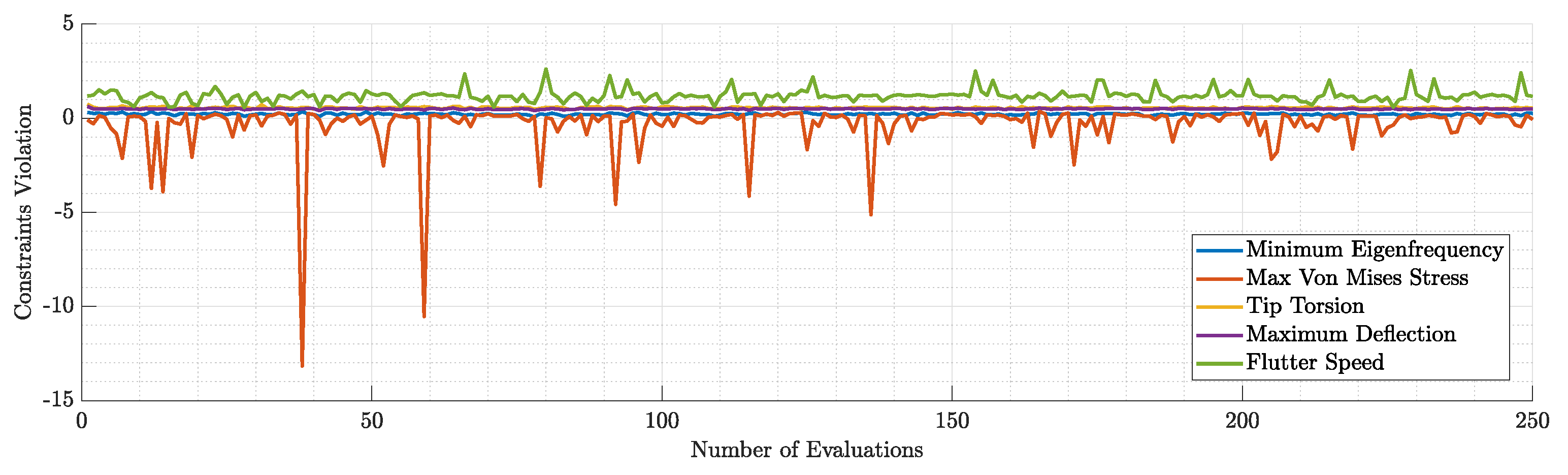
Figure 22.
Objective and constraints violation during the 2nd run.
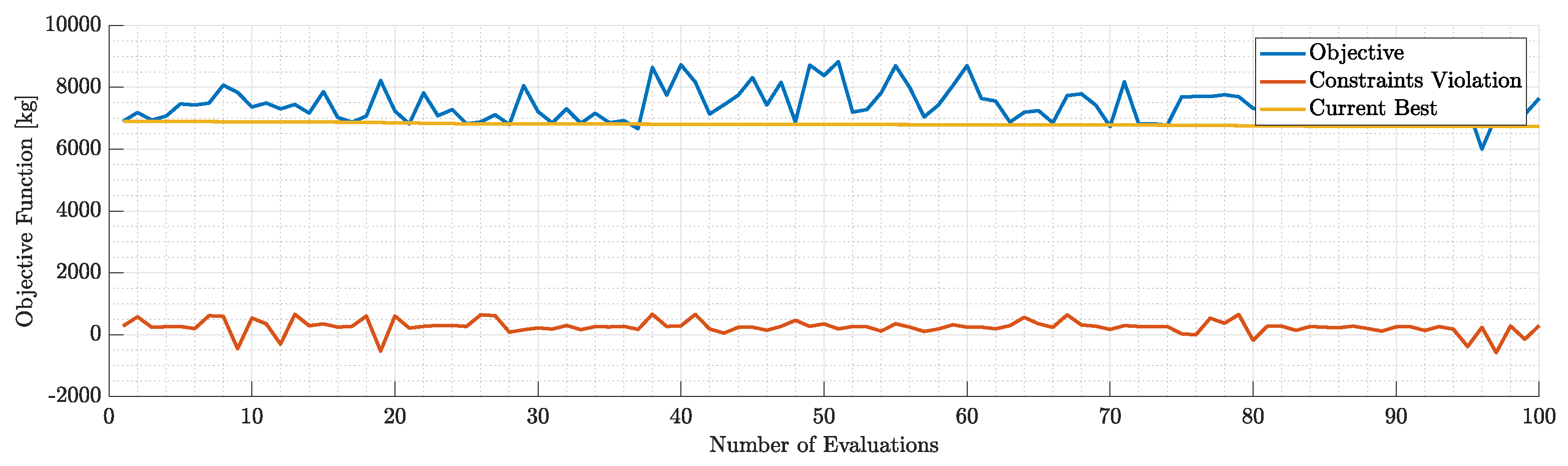
Figure 23.
Violation of each constraint during the 2nd run.
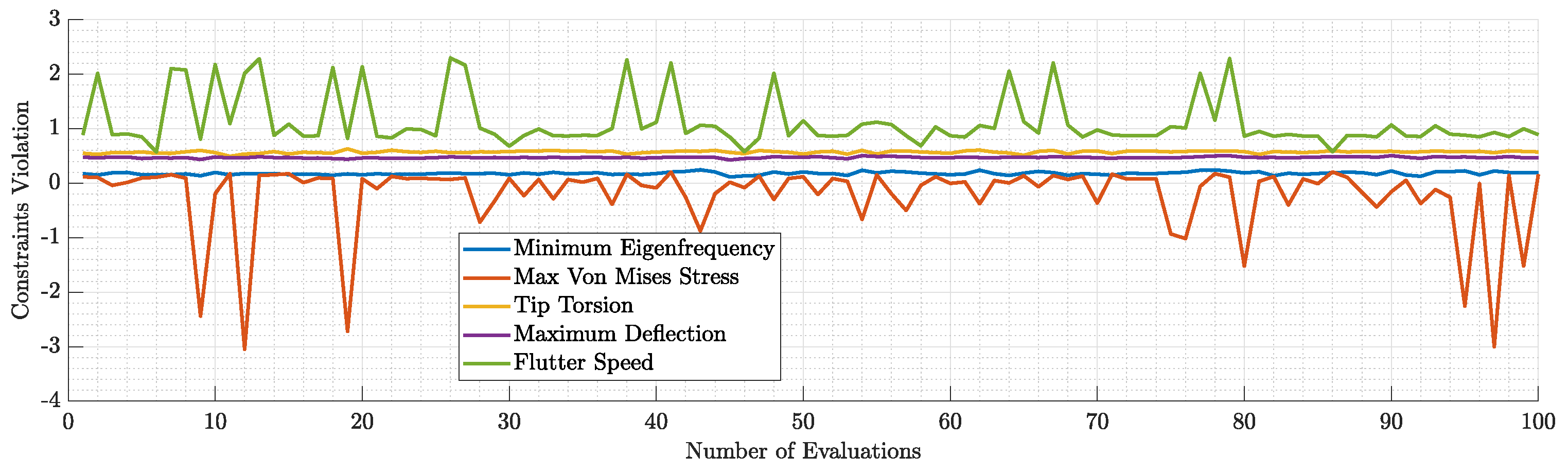
Figure 24.
3D view of the optimized geometry.
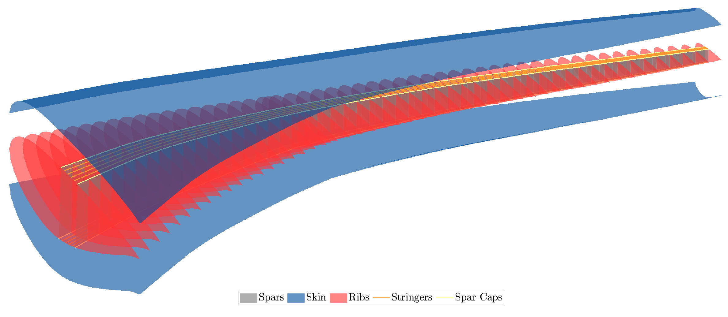
Figure 25.
Optimized thickness distribution of the internal geometry, upper and lower skins along with the corresponding control point values.
Figure 25.
Optimized thickness distribution of the internal geometry, upper and lower skins along with the corresponding control point values.
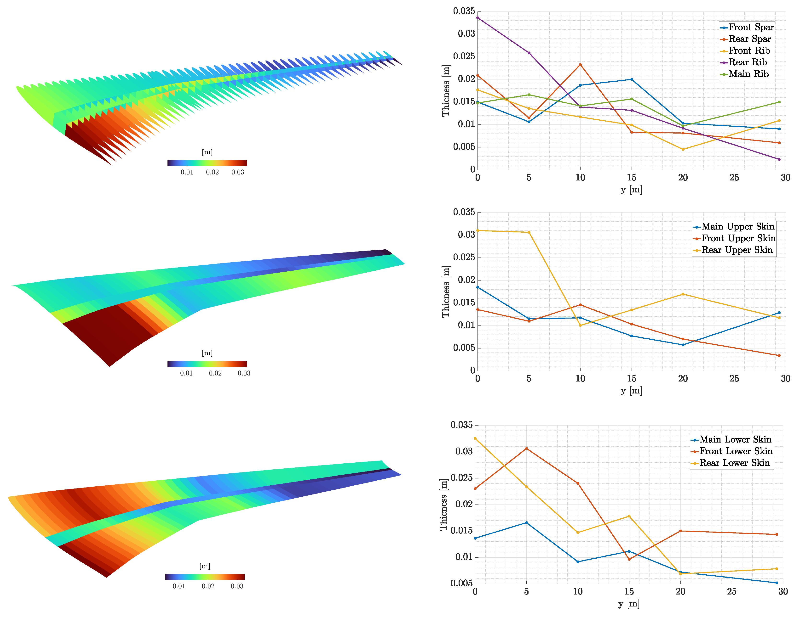
Figure 26.
Displacement distribution of the uCRM wing.
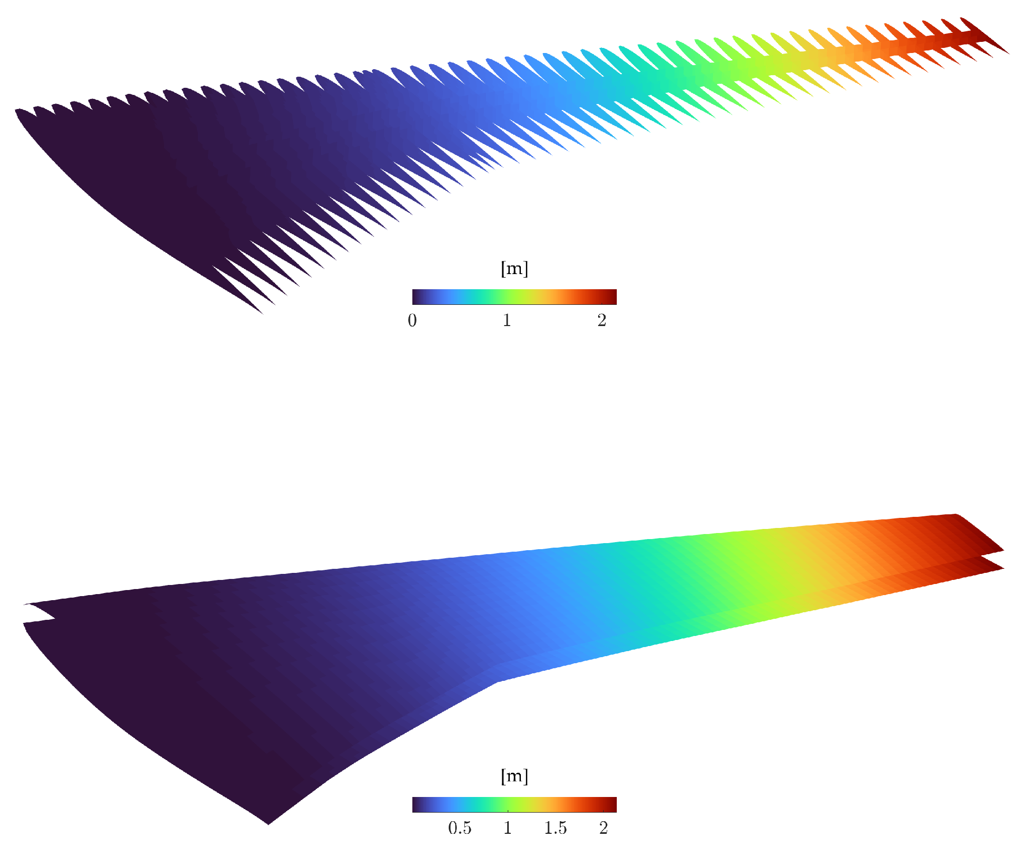
Figure 27.
Wing static aeroelastic displacements.
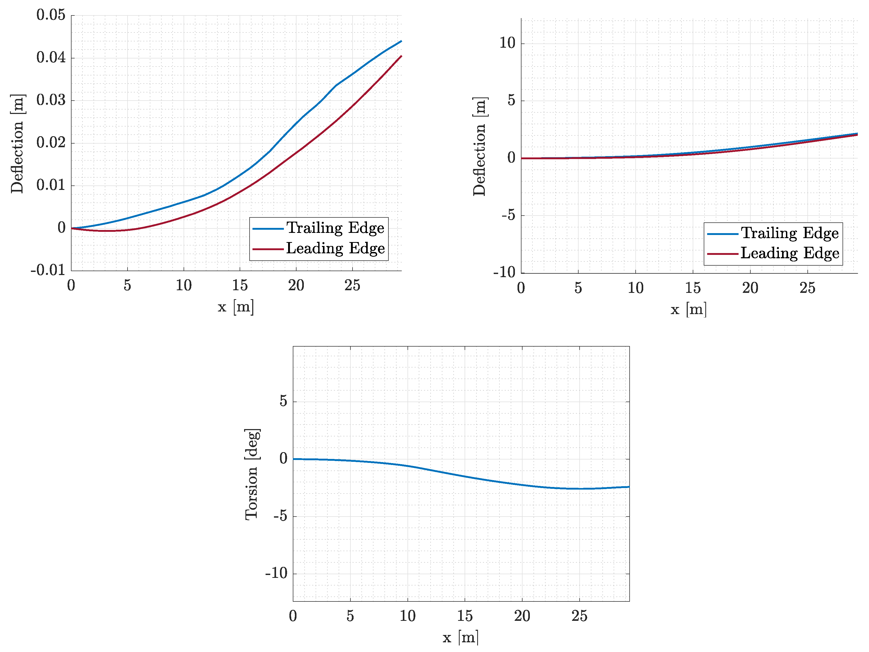
Figure 28.
Von Mises stress distribution of the uCRM wing.
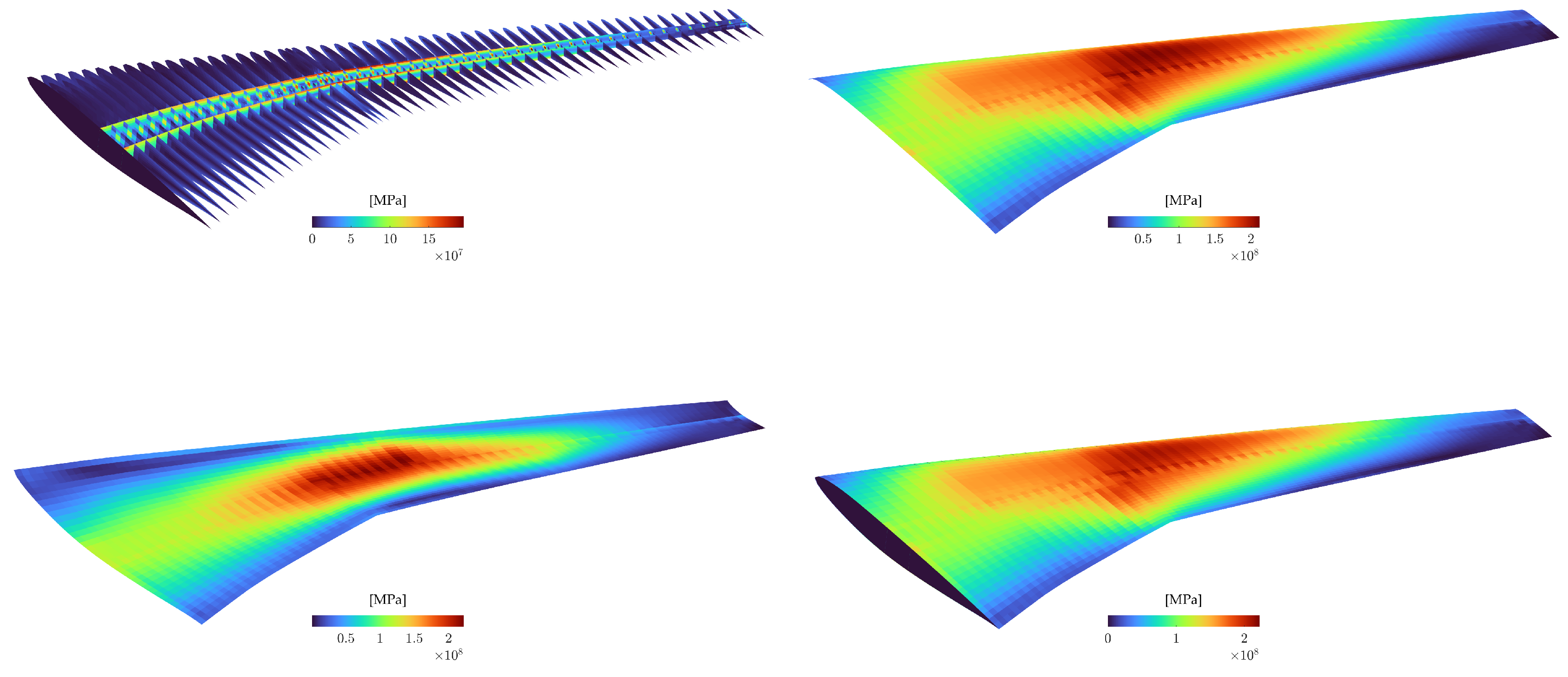
Figure 29.
Coefficient of pressure distribution.
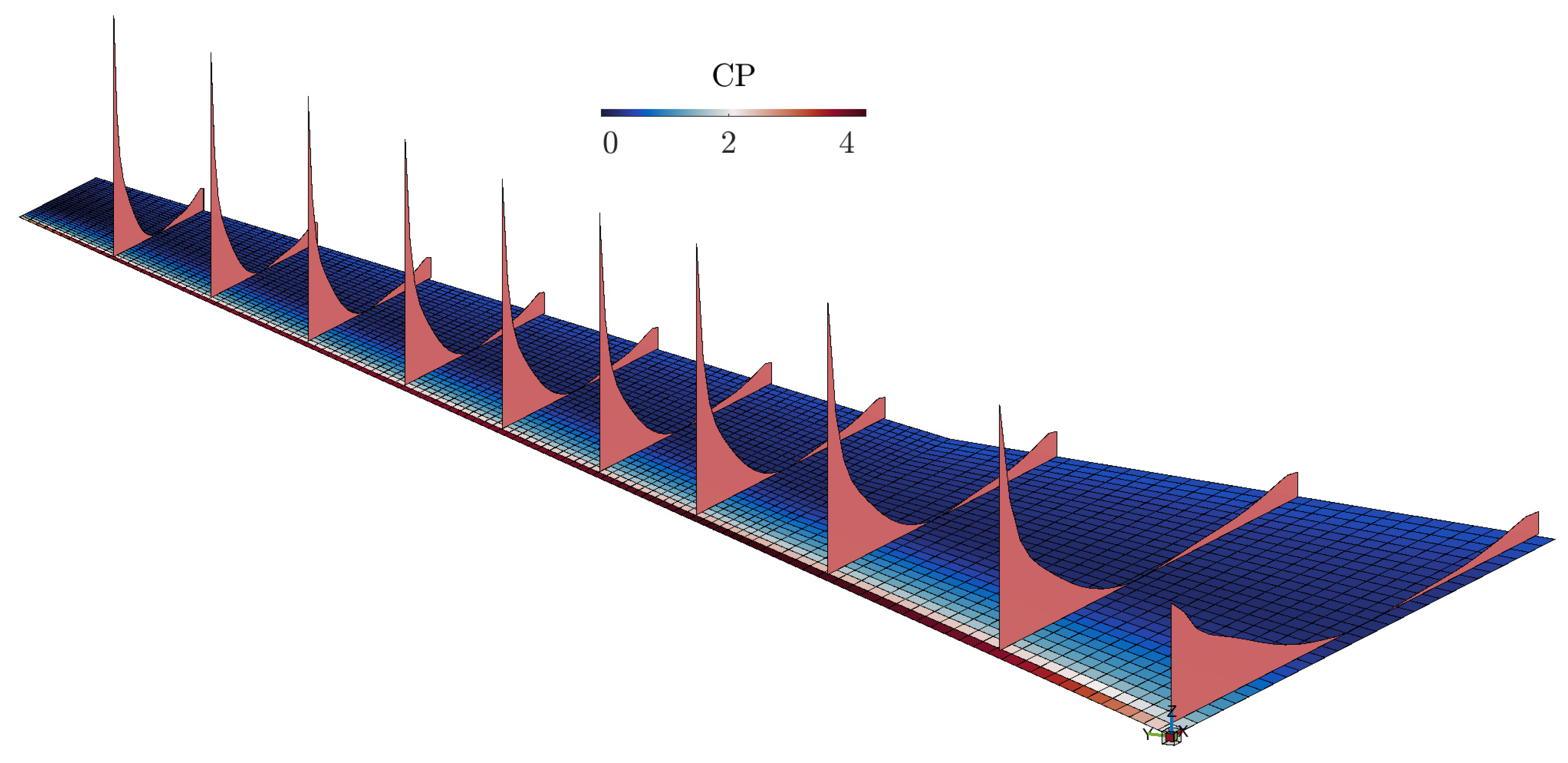
Figure 30.
V-g and V-f plots.
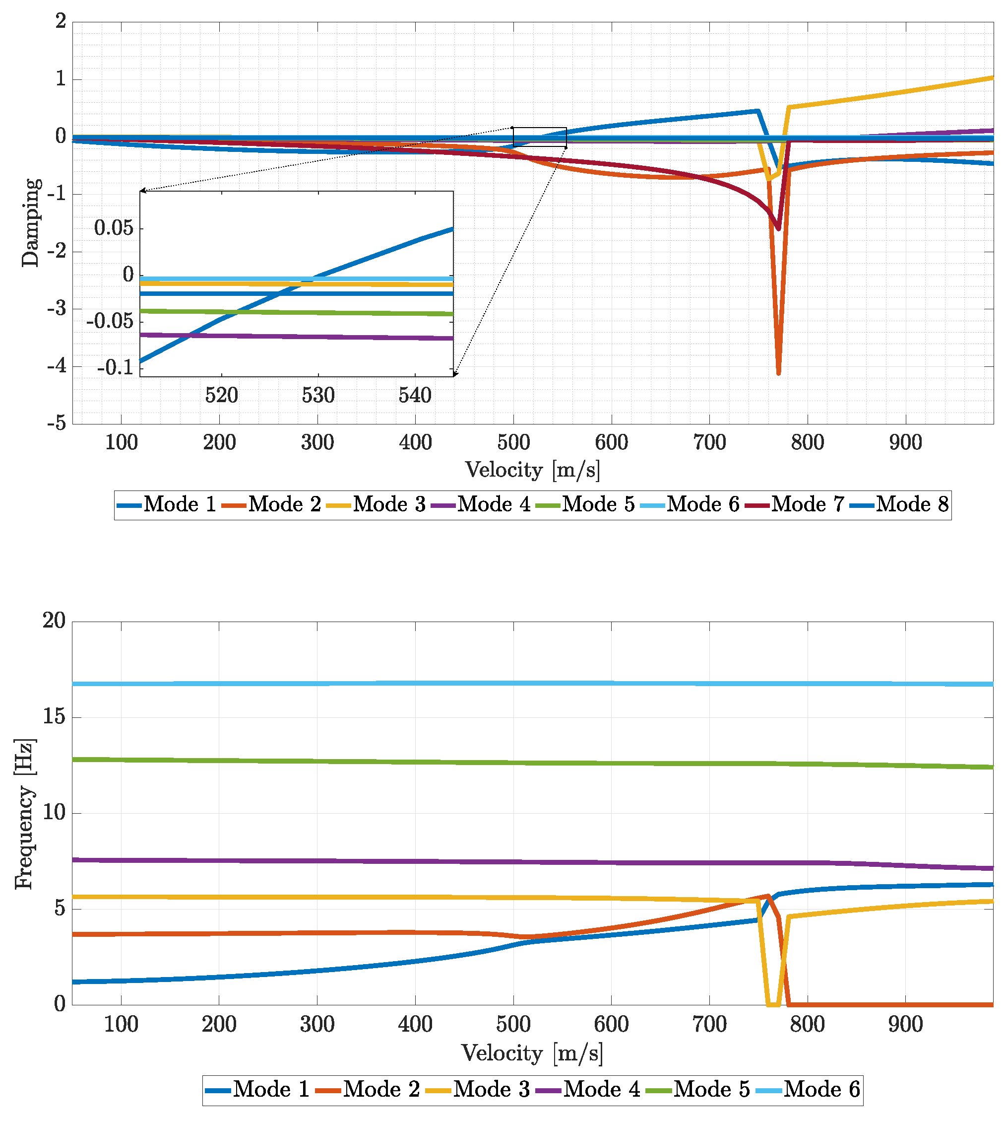
Figure 32.
Objectives during the parallel optimization run.
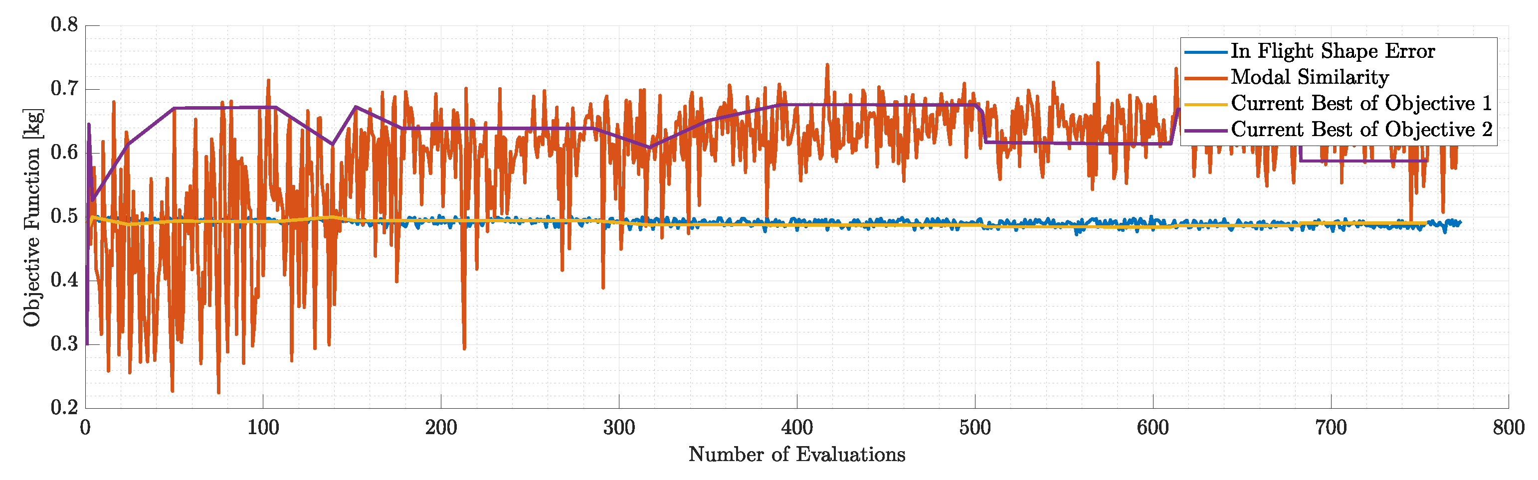
Figure 33.
Violation of each constraint during the parallel optimization run.
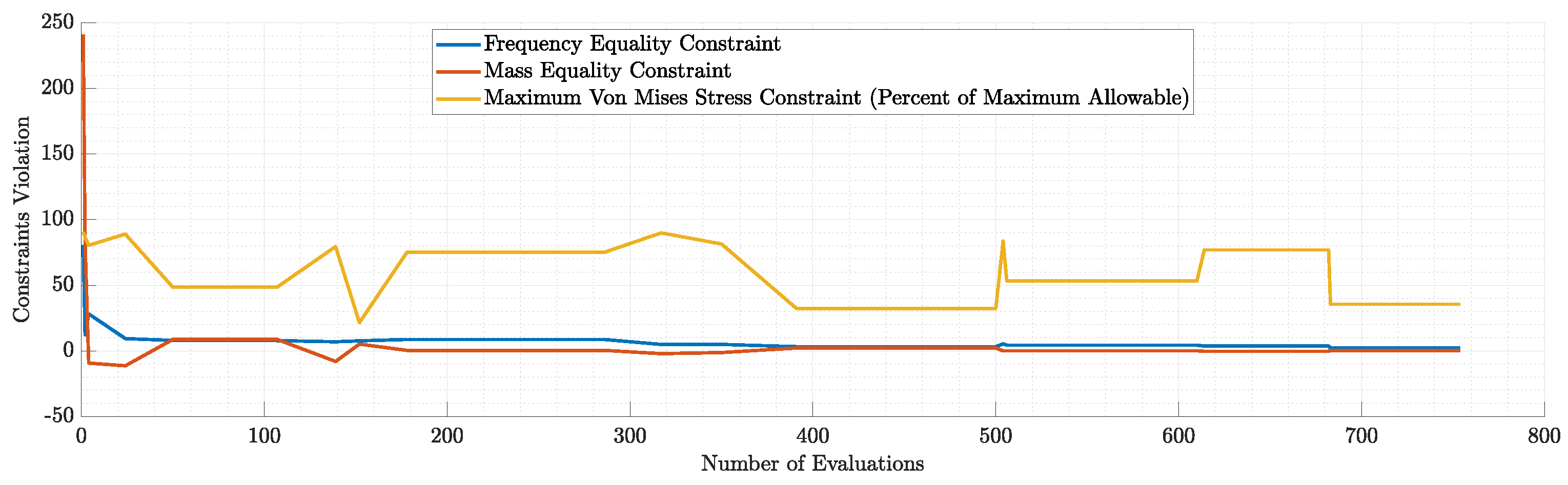
Figure 34.
Objectives during 1st run of static aeroelastic response similarity optimization.
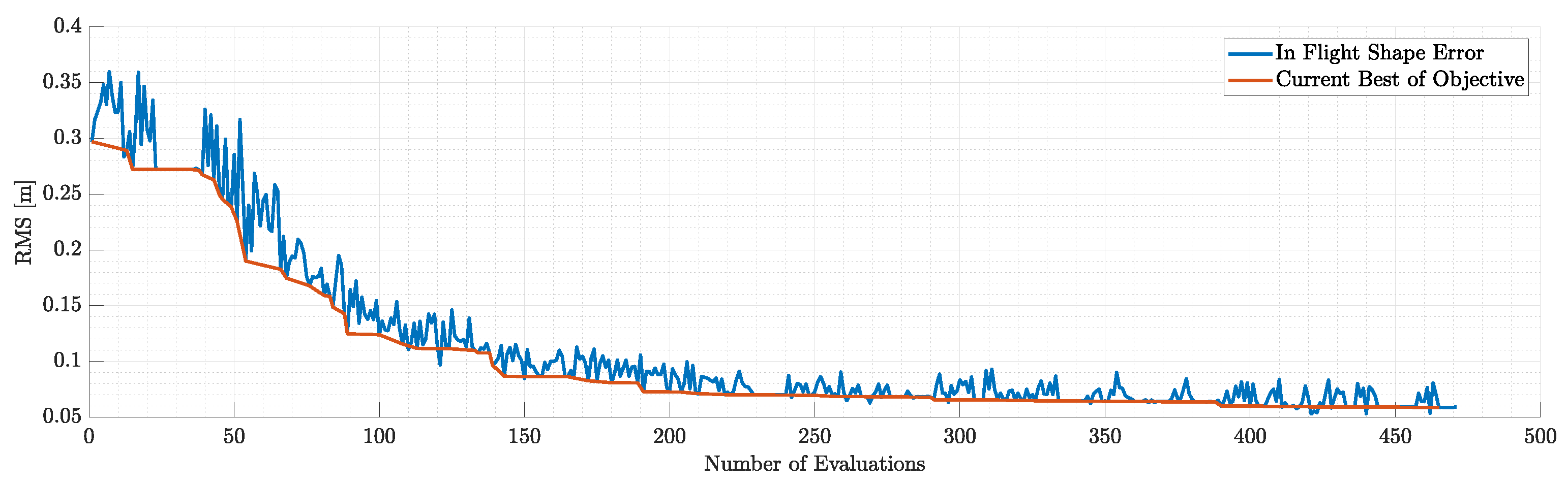
Figure 35.
Objectives during 2nd run of static aeroelastic response similarity optimization.
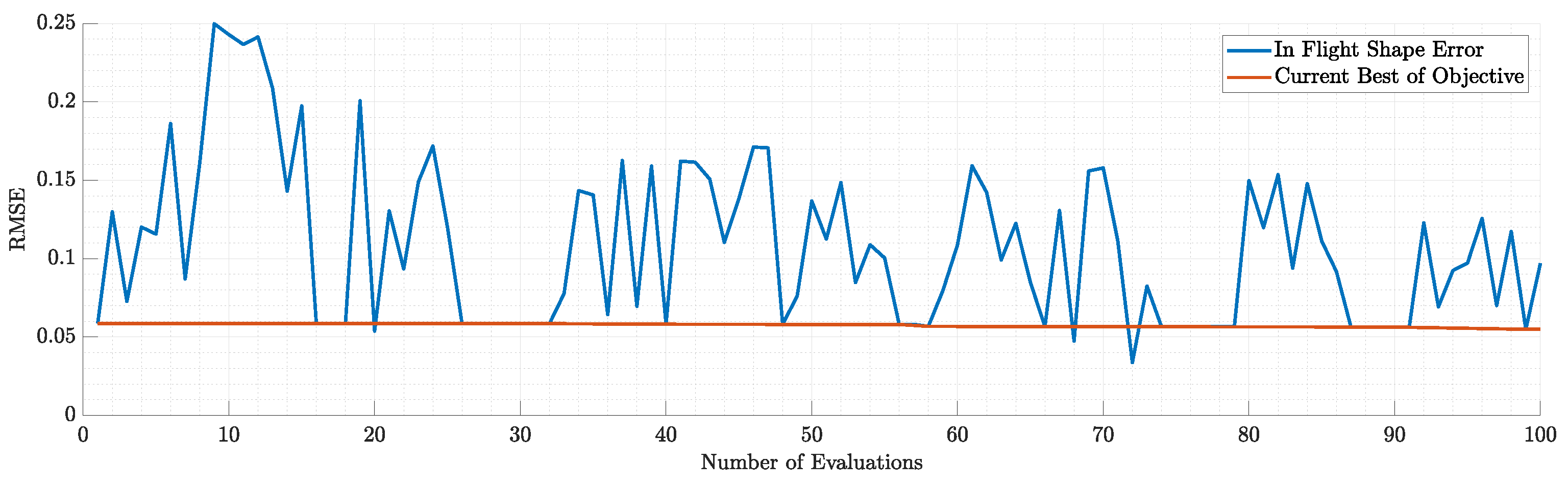
Figure 36.
Optimized thickness distribution of each component and its corresponding control point values for the scaling problem.
Figure 36.
Optimized thickness distribution of each component and its corresponding control point values for the scaling problem.
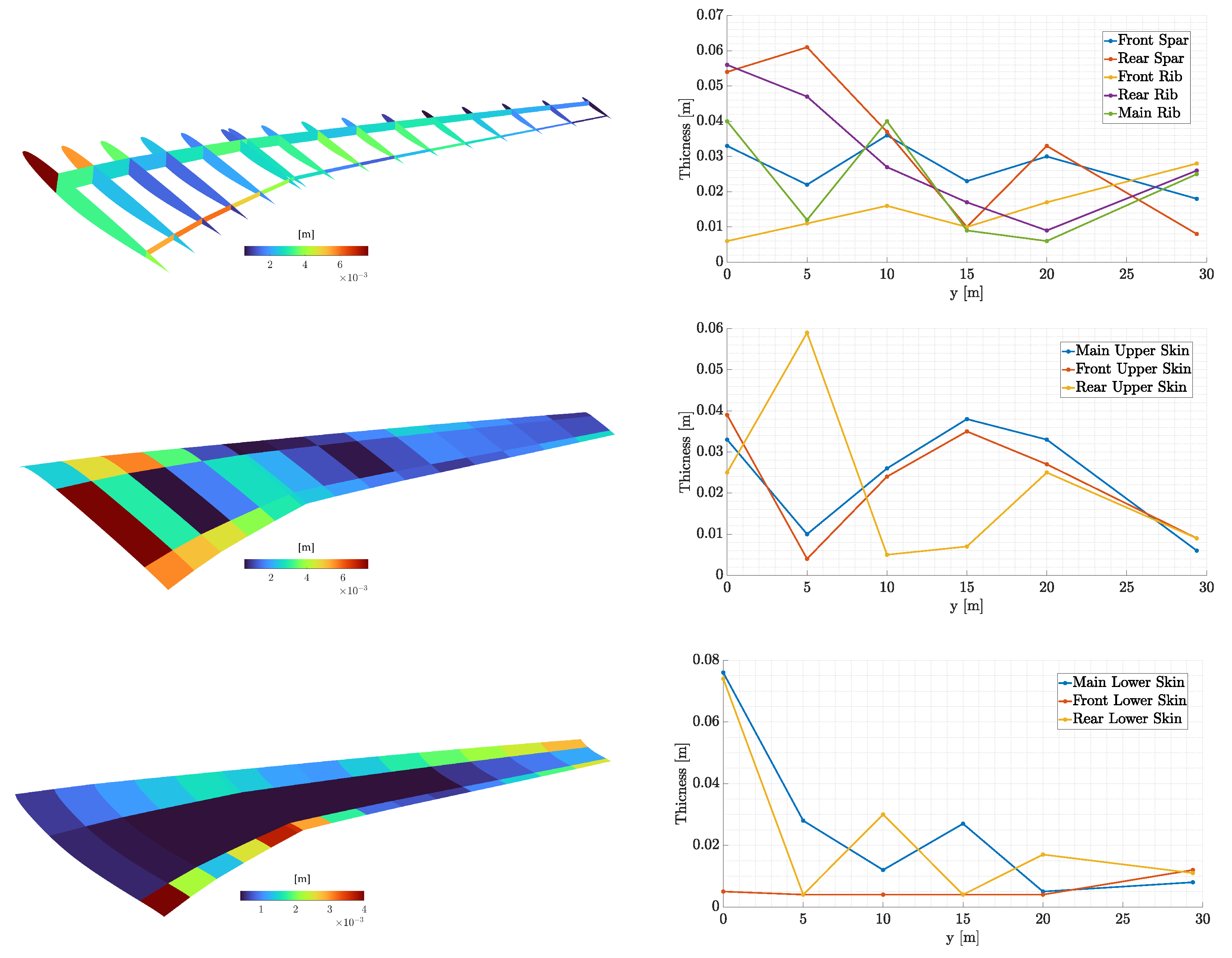
Figure 37.
In-flight aerodynamic surface of the optimized design compared to the target shape.
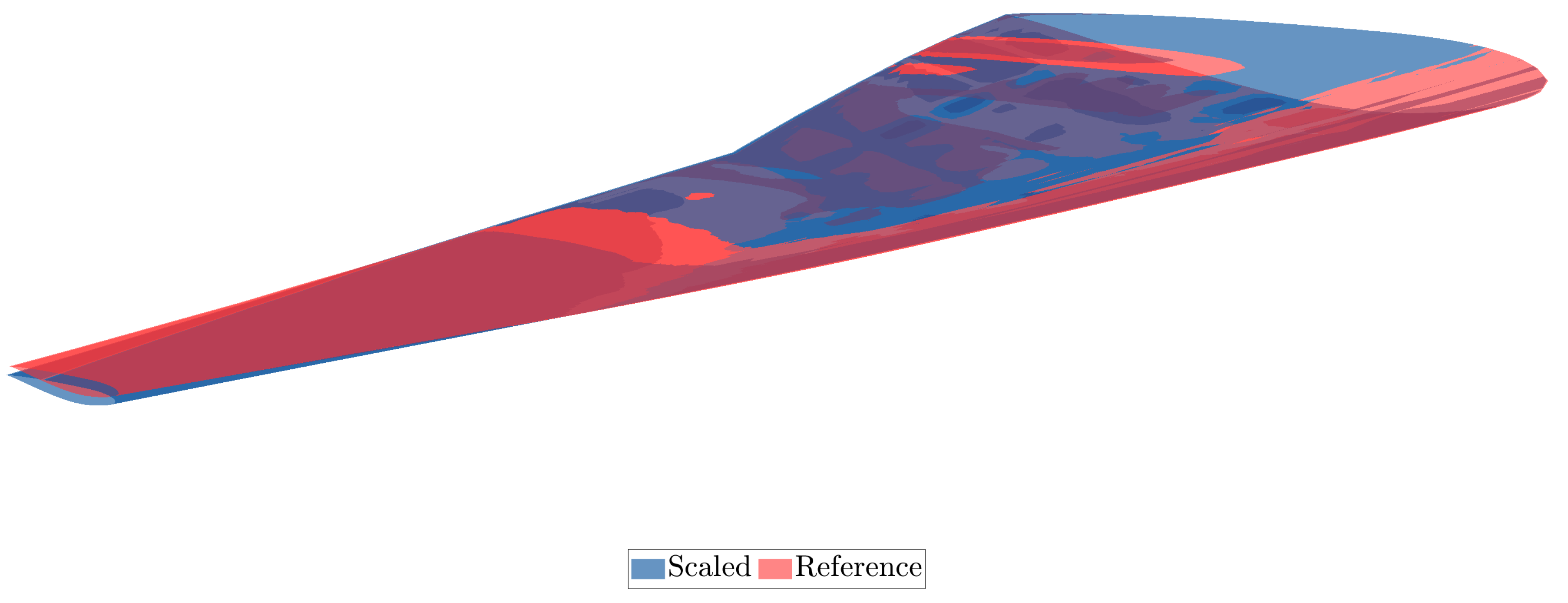
Figure 38.
Comparison of the scaled and reference wing.
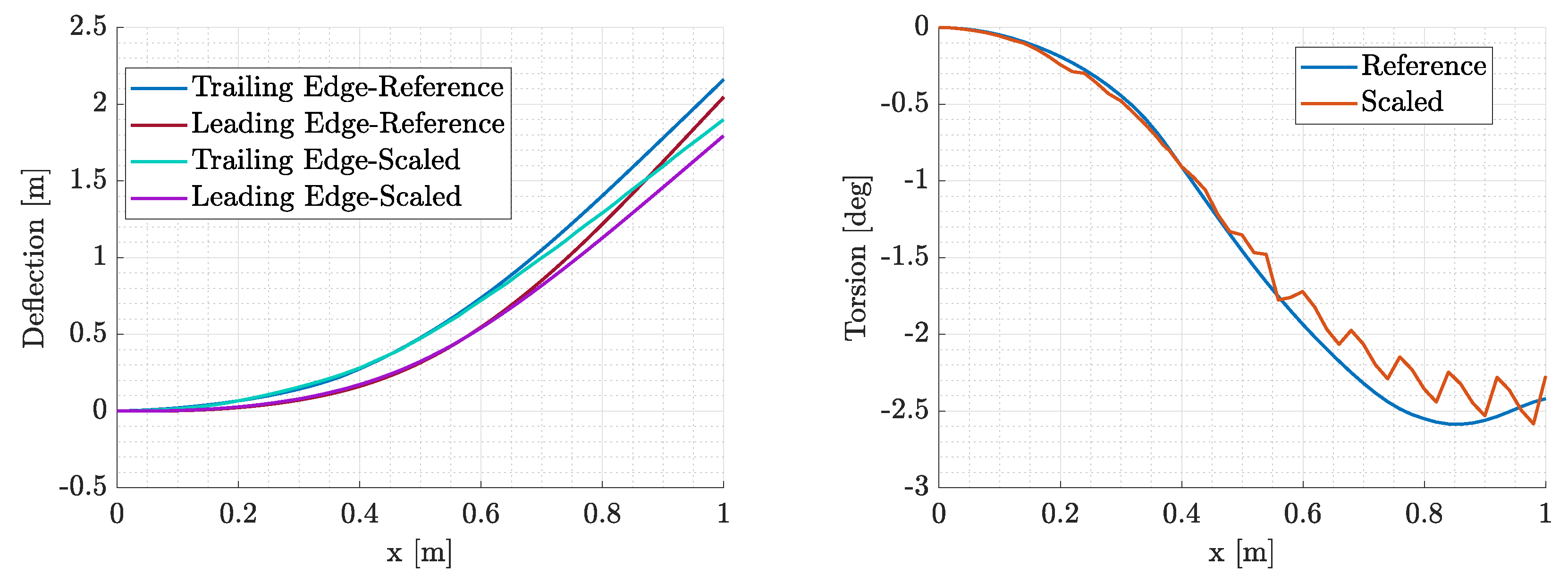
Figure 39.
Von Mises stress distribution of the scaled model.
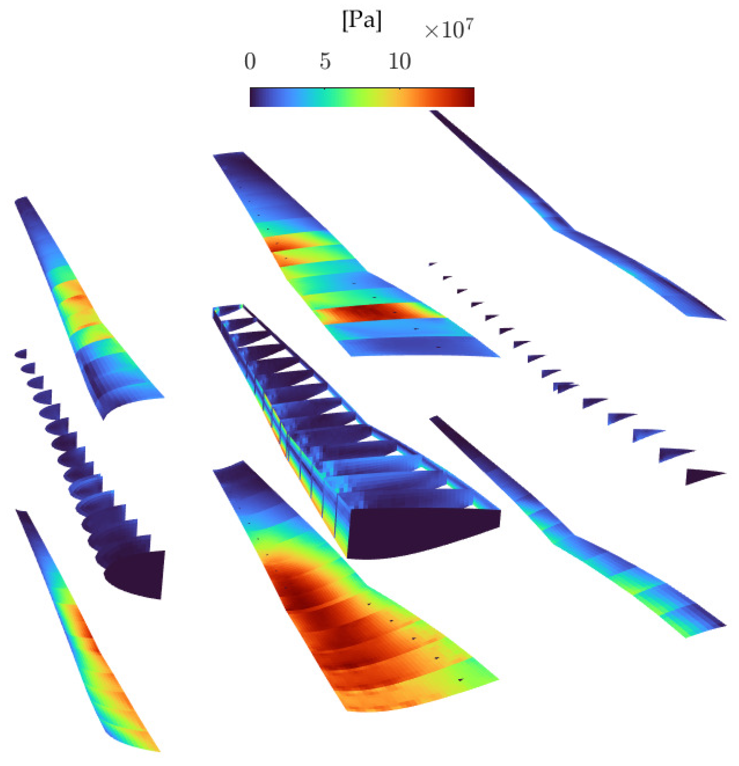
Figure 40.
Objectives during the run of modal similarity optimization for N=5 modes.
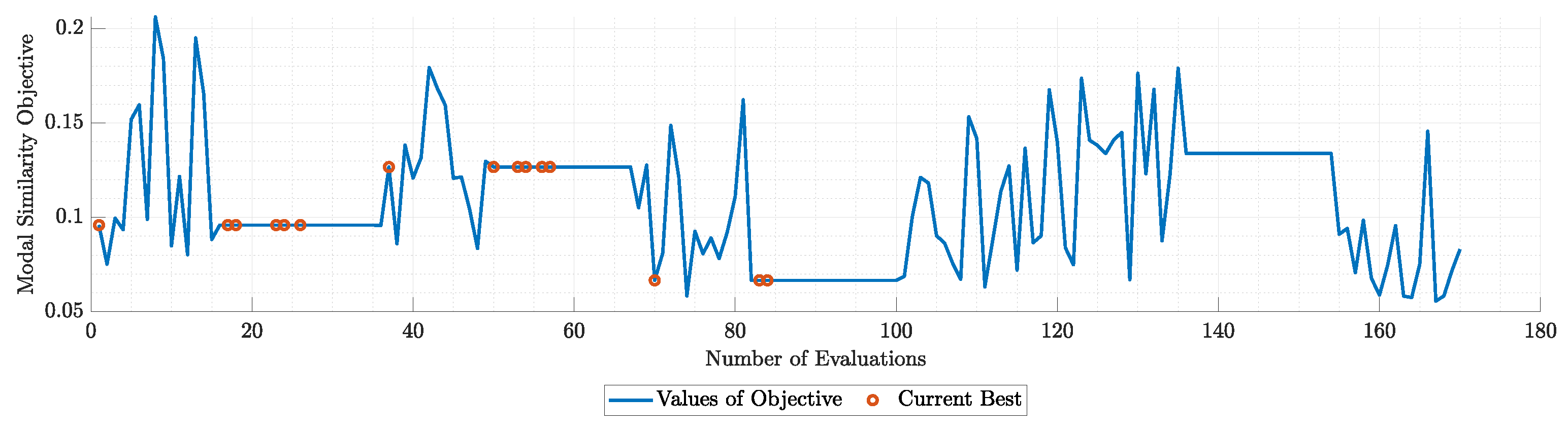
Figure 41.
Violation of each constraint during the run of modal similarity optimization for N=5 modes.
Figure 41.
Violation of each constraint during the run of modal similarity optimization for N=5 modes.
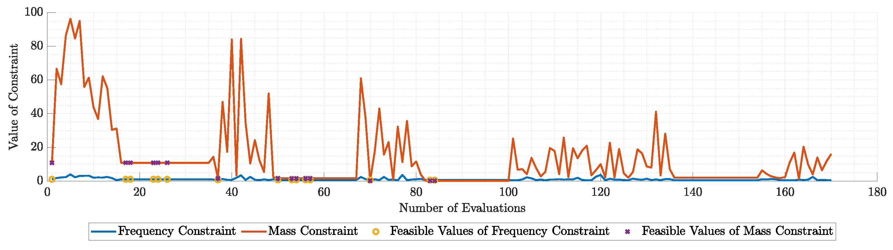
Figure 42.
Optimized lumped masses of the scaled model.
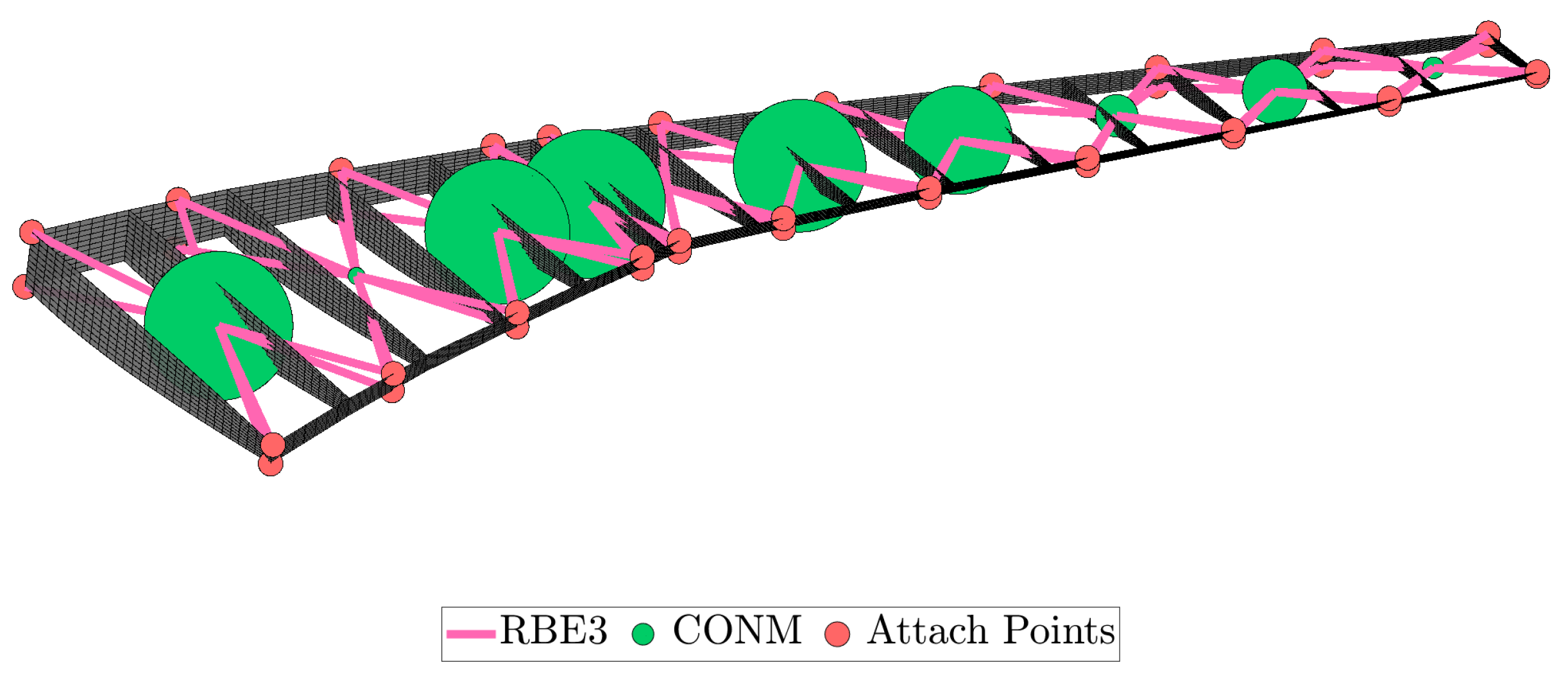
Figure 43.
First eight eigenmodes of the scaled model compared to the modes of the reference wing (red indicates undeformed shape and blue indicates the deformed shape).
Figure 43.
First eight eigenmodes of the scaled model compared to the modes of the reference wing (red indicates undeformed shape and blue indicates the deformed shape).
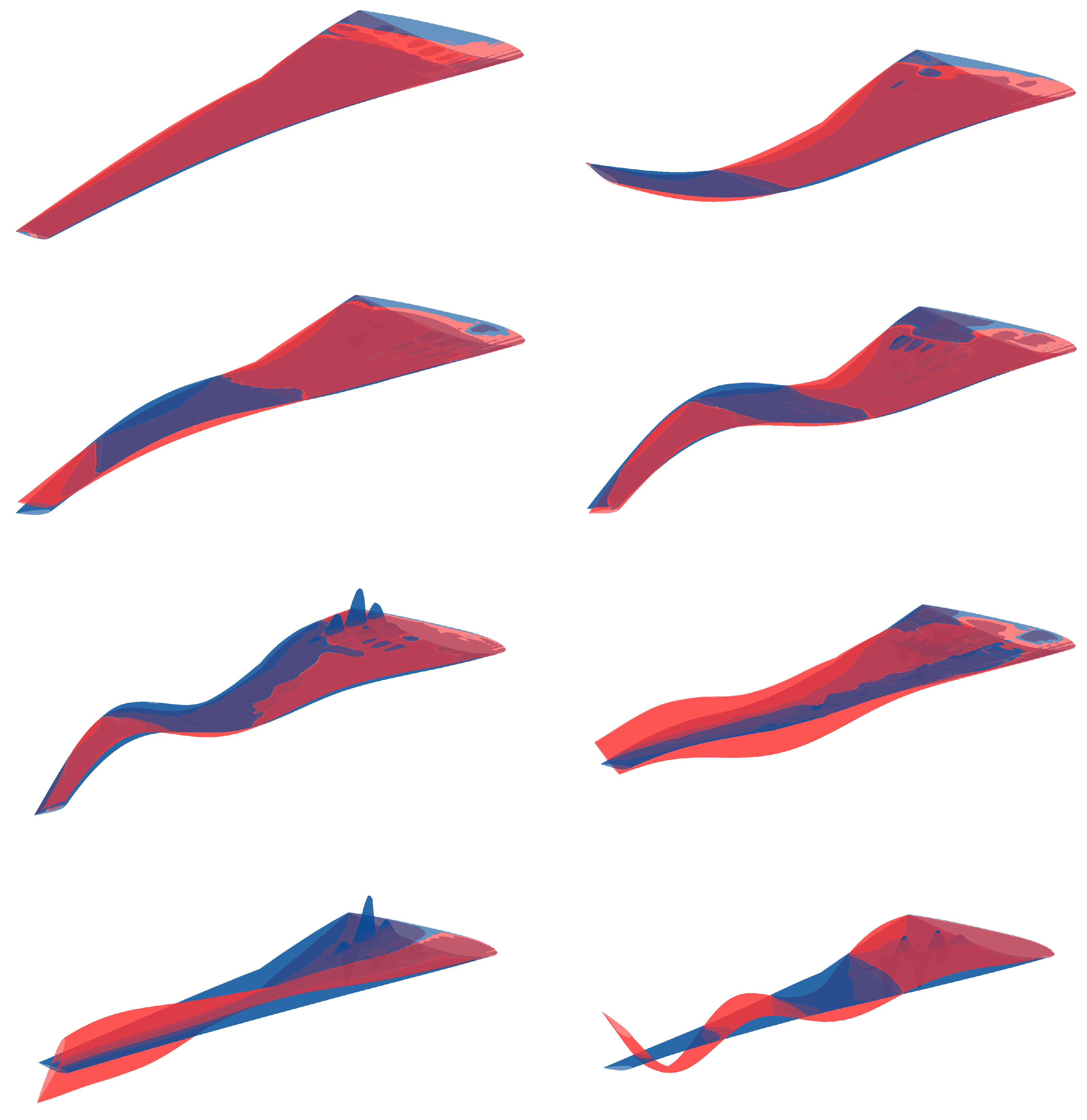
Figure 44.
Objectives during the run of modal similarity optimization for N=10 modes.
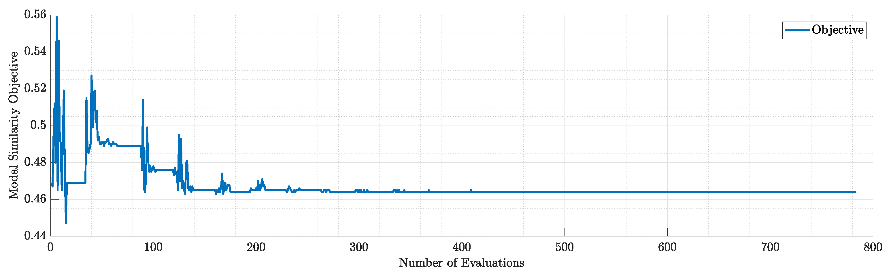
Figure 45.
Violation of each constraint during the run of modal similarity optimization for N=10 modes.
Figure 45.
Violation of each constraint during the run of modal similarity optimization for N=10 modes.
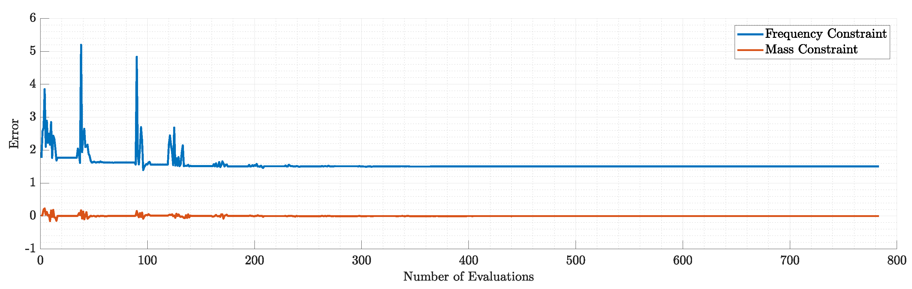
Figure 46.
Flutter results of the optimized scaled wing.
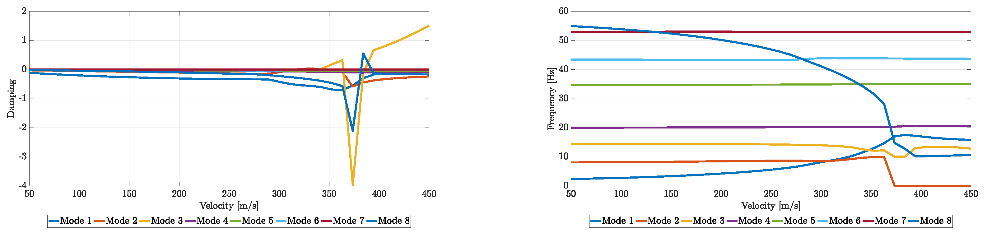
Figure 47.
Spars’ position during the 1st run of static aeroelastic response optimization.
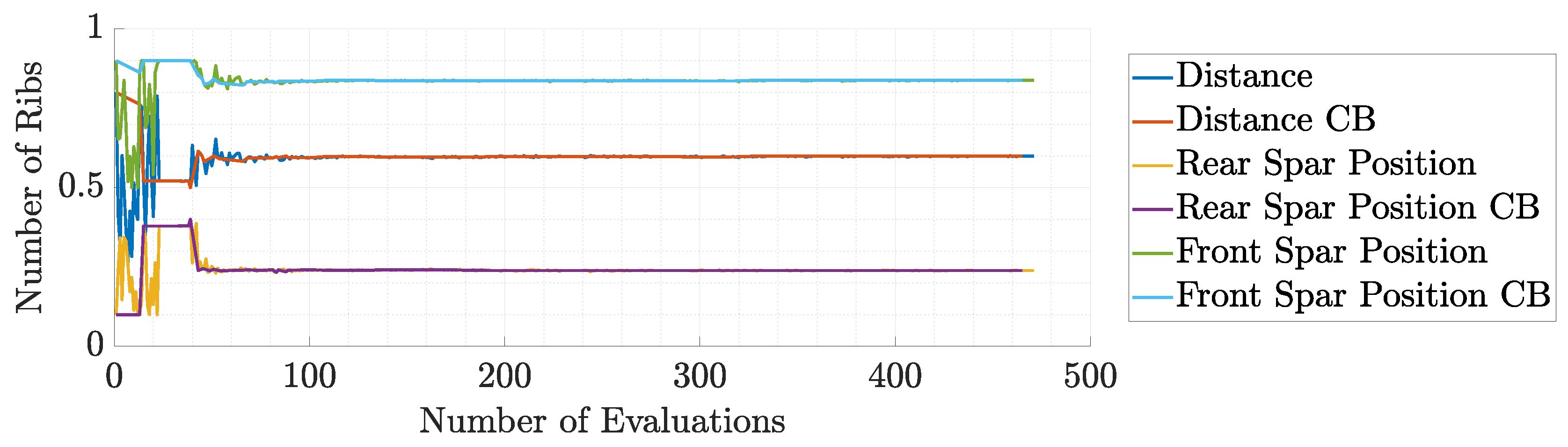
Figure 48.
Number of ribs during the 1st run of static aeroelastic response optimization.
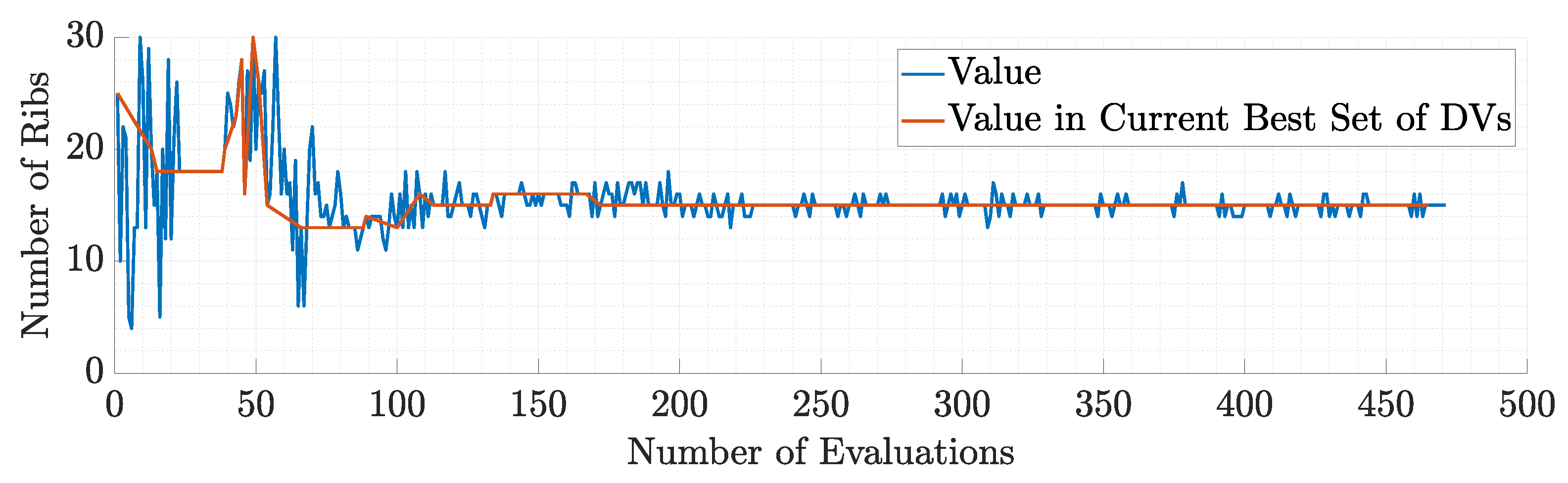
Table 1.
A summary of the features of the publications referenced in this work.
| Author | Aerodynamic | Structural | Optimization | Thicknesses | Topology |
| French and Eastep | DLM | Beam FEM | Gradient | ✓ | ✗ |
| Richards et al. | Thin Airfoil | Shell FEM | Both | ✓ | ✗ |
| Ricciardi et al. | VLM | Shell FEM | Gradient | ✓ | ✗ |
| Ricciardi et al. | VLM | Shell FEM | Gradient | ✓ | ✗ |
| Pontillo et al. | Strip Theory | Beam FEM | Gradient | ✓ | ✗ |
| Spada et al. | DLM | NL Shell FEM | Gradient | ✓ | ✗ |
| Mas Colomer et al. | Panel | Shell FEM | Gradient-Free | ✓ | ✗ |
Table 2.
Aluminium’s mechanical properties.
| Quantity | Value | Units |
|---|---|---|
| Density | 2780 | kg/m3 |
| Young’s modulus | 73.1 | GPa |
| Poisson ratio | 0.3 | - |
| Yield strength | 420 | MPa |
Table 3.
CRM geometric specifications.
| Parameter | uCRM-9 | Units |
|---|---|---|
| Aspect Ratio | 9.0 | - |
| Span | 58.76 | m |
| Side of body chord | 11.92 | m |
| Yehudi chord | 7.26 | m |
| MAC | 7.01 | m |
| Tip chord | 2.736 | m |
| Wimpress reference area | 383.78 | |
| Gross area | 412.10 | |
| Exposed area | 337.05 | |
| 1/4 chord sweep | 35 | deg |
| Taper ratio | 0.275 | - |
Table 4.
CRM wing critical loading conditions.
| Condition | Lift Constraint | Mach Number | Altitude (m) |
|---|---|---|---|
| 2.5G Maneuver | 2.5 MTOW | 0.64 | 0 |
Table 5.
Objectives and constraints of the mass minimization problem.
| Objective | Target |
|---|---|
| Mass | Minimization |
| under the constraints | |
| Maximum Deflection | |
| Tip Torsion Angle | deg |
| First Eigenfrequency | ≥ 1 Hz |
| Maximum Von Mises Stress | ≤ 280 MPa |
| Flutter Speed | |
Table 6.
Design variables of the optimization problem.
| Variable | Lower Bound | Upper Bound | Dimension |
|---|---|---|---|
| Ribs Number | 6 | 52 | 1 |
| Stringers Number | 4 | 12 | 1 |
| Front Spar Position | 0.1 | 0.4 | 1 |
| Rear Spar Position | 0.5 | 0.9 | 1 |
| Stringer and Spar Cap Thickness | 1 mm | 10 mm | 2 mm |
| Thicknesses at Control Points | 2 mm | 40 mm | 66 mm |
Table 7.
MIDACO parameters.
| Run | Iterations | Accuracy | FOCUS | Initial Point |
|---|---|---|---|---|
| 1 | 250 | 0.1 | 0 | Random |
| 2 | 100 | 0.01 | 10 | Run 1 |
Table 8.
optimization results summary.
| Property | Value |
|---|---|
| Mass | 6902 kg |
| Minimum Eigenfrequency | 1.1735 Hz |
| Maximum Von Mises Stress | 247.5 MPa |
| Tip Torsion | 2.7 deg |
| Maximum Deflection | 7.89% of span or 2.32 m |
| Flutter Speed | 501 m/s |
Table 9.
Optimized geometric design variables.
| Variable | Value |
|---|---|
| Ribs Number | 51 |
| Stringers Number | 4 |
| Front Spar Position | 0.3904 |
| Rear Spar Position | 0.5166 |
| Stringer Thickness | 2 mm |
| Spar Cap Thickness | 3 mm |
Table 10.
Objectives and constraints of the scaling problem.
| Objective | Target |
|---|---|
| In-Flight Shape Difference | Minimization |
| Modal Similarity (MAC) | Maximization |
Table 11.
Objectives and constraints of the mass minimization problem.
| Constraint | Target |
|---|---|
| Frequency Difference | |
| Overall Mass | |
| Maximum Von Mises Stress |
Table 12.
Target values of frequency for the optimization problem.
| Mode Number | Reference Wing Frequency, Hz | Scaled Wing Frequency, Hz |
|---|---|---|
| 1 | 1.1915 | 2.6642 |
| 2 | 3.7067 | 8.2885 |
| 3 | 5.6416 | 12.6151 |
| 4th | 7.58 Hz | 16.9494 |
| 5th | 12.8288 | 28.6861 |
| 6th | 16.7503 | 37.4548 |
| 7th | 17.9140 | 40.0570 |
| 8th | 19.4901 | 43.5812 |
Table 14.
Magnesium’s mechanical properties.
| Quantity | Value | Units |
|---|---|---|
| Density | 1800 | |
| Young’s modulus | 45 | |
| Poisson ratio | 0.35 | - |
| Yield strength | 150 |
Table 15.
MIDACO parameters of the static aeroelastic response similarity optimization.
| Run | Iterations | Accuracy | FOCUS | Initial Point |
|---|---|---|---|---|
| 1 | 500 | 0.1 | 0 | Random |
| 2 | 100 | 0.01 | 10 | Run 1 |
Table 16.
Optimized geometric design variables.
| Variable | Value |
|---|---|
| Ribs Number | 15 |
| Stringers Number | 5 |
| Front Spar Position | 0.239 |
| Rear Spar Position | 0.839 |
Table 17.
Optimized mass values for the modal response similarity optimization problem.
| Mass | Value [kg] |
|---|---|
| 1 | 79.78 |
| 2 | 9.13 |
| 3 | 77.79 |
| 4 | 79.86 |
| 5 | 0.01 |
| 6 | 71.07 |
| 7 | 58.12 |
| 8 | 22.79 |
| 9 | 35.20 |
| 10 | 11.64 |
Table 18.
Target values of frequency for the optimization problem.
| Mode Number | Target | Optimized | Error |
|---|---|---|---|
| 1 | 14.63 % | ||
| 2 | 2.39 % | ||
| 3 | 14.60 % | ||
| 4 | 18.84 % | ||
| 5 | 21.76 % |
Disclaimer/Publisher’s Note: The statements, opinions and data contained in all publications are solely those of the individual author(s) and contributor(s) and not of MDPI and/or the editor(s). MDPI and/or the editor(s) disclaim responsibility for any injury to people or property resulting from any ideas, methods, instructions or products referred to in the content. |
© 2024 by the authors. Licensee MDPI, Basel, Switzerland. This article is an open access article distributed under the terms and conditions of the Creative Commons Attribution (CC BY) license (http://creativecommons.org/licenses/by/4.0/).
Copyright: This open access article is published under a Creative Commons CC BY 4.0 license, which permit the free download, distribution, and reuse, provided that the author and preprint are cited in any reuse.


