
Submitted:
30 March 2025
Posted:
31 March 2025
You are already at the latest version
Abstract
This paper presents a multi-fidelity optimization procedure for aircraft wing design, implemented in the early stages of the aircraft design process. Since wing shape is a key factor influencing aerodynamic performance, having an accurate estimate of its efficiency at the conceptual design phase is highly beneficial for aircraft designers. This study introduces a comprehensive optimization framework for designing the wing of a Class I fixed-wing mini-UAV with electric propulsion, focusing on maximizing aerodynamic efficiency and operational performance. Utilizing Class Shape Transformation (CST) in combination with Surrogate-Based Optimization (SBO) techniques, the research first optimizes the airfoil shape to identify the most suitable airfoil for the UAV wing. Subsequently, SBO techniques are applied to generate wing geometries with varying characteristics, including aspect ratio (AR), taper ratio (λ), quarter-chord sweep angle (Λ0.25), and tip twist angle (ε). These geometries are then evaluated using both low- and high-fidelity aerodynamic simulations. The integration of SBO techniques enables an efficient exploration of the design space while minimizing computational costs associated with iterative simulations. Specifically, the proposed SBO framework enhances the wing’s aerodynamic characteristics by optimizing the lift-to-drag ratio and reducing drag.
Keywords:
Aircraft wings
; Low-fidelity Aerodynamics
; Computational Fluid Dynamics (CFD)
; Aircraft Conceptual Design
; Aircraft Aerodynamics
; Multi-fidelity Optimization
; Surrogate-Based Optimization (SBO)
1. Introduction
The aerodynamic design of aircraft wings plays a crucial role in achieving optimal performance and desirable flight characteristics. Traditionally, wing design follows a multi-stage process, starting from the conceptual design phase and advancing to detailed shape optimization for the final aircraft configuration. Throughout this process, calculations and analyses of variable fidelity are conducted to determine the optimal wing design, ensuring the best possible aerodynamic performance across the aircraft’s flight envelope. A key challenge in aircraft design is accurately estimating performance throughout the entire design process, including the conceptual, preliminary, and detailed design phases. The wing’s aerodynamic efficiency is one of the most critical factors influencing overall aircraft performance, particularly in achieving optimal range and endurance. Since an aircraft’s range is directly related to the lift-to-drag ratio (), optimizing this ratio is crucial. The first and most important step in this process is determining the optimal wing geometry that maximizes . Several geometric parameters affect wing performance, such as aspect ratio (AR), taper ratio (), and quarter-chord sweep angle (). However, the airfoil shape is the most influential factor in determining a wing’s aerodynamic behavior and aircraft designers must carefully select the ideal airfoil early in the design process to ensure optimal performance.
Over the past decades, numerous studies have investigated various aspects of wing aerodynamic optimization. Starting with airfoil optimization, researchers have explored different parameterization techniques, such as Class-Shape Transformation (CST), PARSEC, and Bézier curves. Salunke et al. [1] reviewed existing airfoil parameterization techniques, concluding that a combination of Bézier and PARSEC methods provides broad coverage of different airfoil designs. The airfoil optimization using swarm algorithms with mutation and artificial neural networks, establishing a relationship between mapped PARSEC solution space and aerodynamic coefficients was explored in [2]. Masters et al. [3] provided a comprehensive review of seven airfoil shape parameterization methods, including CST, B-splines, Hicks-Henne bump functions, radial basis function domain elements, Bézier surfaces, singular-value decomposition modal extraction, and parameterized sections. Additional researchers ([4,5,6,7,8,9] and [10]) have studied airfoil shape optimization by combining various parameterization techniques to refine well-known airfoils for specific performance requirements.
Similarly, wing aerodynamic shape optimization has been widely explored. Lyu et al. [11] investigated aerodynamic shape optimization of a benchmark wing using a gradient-based optimization algorithm coupled with Reynolds-Averaged Navier–Stokes (RANS) equations and the Spalart–Allmaras turbulence model. Following this study, the aerodynamic shape of the Common Research Model (CRM) wing-body-tail configuration under a trim tail constraint was optimized in Chen et al. [12]. Benaouali and Kachel [13] introduced a multidisciplinary design optimization (MDO) approach for aircraft wings, integrating commercial software tools and first optimizing the airfoil shape using CST before addressing overall wing performance. Other researchers, such as Ghafoorian et al. [14] and Zheng et al. [15], have contributed to the field by focusing on aerodynamic shape optimization—the former optimized wind turbine blades, while the latter applied manifold learning techniques for aerodynamic shape design optimization of wings.
Despite extensive research on airfoil and wing optimization, most existing studies focus on refining established geometries rather than developing truly optimal designs tailored to a specific aircraft’s mission and flight envelope. Moreover, these frameworks are often presented in an isolated manner, leading to a knowledge gap regarding the design parameters as well as the impact of computational fidelity that most significantly influence performance and the resulting optimal aerodynamic design. Moreover, the vast nature of the design variables involved in the aerodynamic design of aircraft wings dramatically increases the number of analyses required to sufficiently explore the design space and to subsequently extract the global optimum configuration. This situation is exacerbated when considering the inclusion of high-fidelity aerodynamic analyses such as CFD. In order to alleviate the computational burden and to sufficiently explore the design space without compromising the quality of the results, surrogate modeling algorithms are often employed in the design of engineering systems [16,17,18,19]. Such models provide rapid prediction of performance metrics, balancing computational feasibility with accuracy.
Aiming to bridge this gap in the literature, the goal of this study is to determine the optimal wing geometry based on the aircraft’s unique performance requirements, starting from the early stages of the conceptual design and to assess the influence of the level of fidelity of the aerodynamic analysis tools to the overall wing design and performance. This process begins with the determination of the primary wing performance and geometrical parameters using classical conceptual design tools. An assumed maximum lift coefficient is used in the generation of the constraint diagram of the aircraft. As a next step, the proposed methodology integrates the CST parameterization with low-fidelity aerodynamics (XFOIL) and Surrogate-Based Optimization (SBO) to identify the optimal airfoil. This selection is based on achieving the assumed maximum lift coefficient while ensuring high performance at low Reynolds numbers, which characterize the aircraft’s operational conditions.
In the first optimization framework, following the selection of the optimal airfoil, a low-fidelity optimization process is conducted using SBO in conjunction with low-fidelity aerodynamics simulations (panel method - XFLR5). This phase aims to determine the optimal wing geometry by maximizing the lift-to-drag ratio () while imposing constraints on the lift-curve slope ( ), stall Angle of Attack (AoA) (), and at zero AoA. The optimization considers four key geometric parameters: aspect ratio (AR), taper ratio (), quarter-chord sweep angle (), and tip twist angle (). Subsequently, a third SBO framework is employed using high-fidelity aerodynamics simulations (Ansys Fluent CFD). The design space is refined by adapting the upper and lower boundaries based on the optimal wing geometry obtained from the low-fidelity SBO. An additional constraint is introduced for the maximum lift coefficient (), ensuring that the final design meets performance expectations under high-fidelity simulations.
In order to assess the possibility of using high-fidelity CFD analysis and the accuracy of the low-fidelity numerical tools, along with their impact on the optimal wing geometry, a second SBO framework is considered. This optimization process considers high-fidelity CFD aerodynamics, applied immediately after the airfoil optimization phase, bypassing the intermediate low-fidelity wing optimization. The objective and constraints remain the same as those in the third phase of the first framework, with identical upper and lower geometric boundaries to the second phase of the first framework. The optimal wing geometry of this second framework is then compared with the result of the first framework to assess the effectiveness and accuracy of both approaches.
2. Materials and Methods
2.1. Baseline Aircraft Specifications and Requirements
The design process begins with the definition of the mission flight characteristics and the operational requirements of the aircraft. Within the framework of this study, an Unmanned Aerial Vehicle (UAV) has been selected as the case study. According to the NATO classification system for UAVs, the aircraft in this study falls into the Class I mini UAV category. Table 1 presents the key UAV parameters that serve as the basis for the aerodynamic optimization and design framework.
2.2. Conceptual Design Methodology
For the conceptual wing design, a methodology based on Raymer’s [20] and Roskam’s [21] design approaches was adopted and modified to meet the specific requirements of a Class I mini-UAV with electric propulsion. The process begins with determining the UAV’s final takeoff weight using Equations (1, 2, and 3), based on the initial design specifications.
where:
- is the guessing take-off weight,
- is the payload weight,
- is the battery weight,
- is the calculated take-off weight based on the guess, payload and battery weights,
- is the empty weight fraction,
- is the calculated take-off weight.
Next, a constraint diagram of the aircraft is developed based on key design criteria, including stall speed (Equation(4)), catapult takeoff (Equation(5)), rate of climb, climb gradient (Equation(6)), and sustained turn (Equation(7)). This diagram helps in selecting the optimal wing loading and power loading, which serve as key parameters in guiding the aircraft’s design. To construct the constraint diagram, in addition to the aircraft specifications, certain assumptions are made regarding the airfoil used for the wing, such as its maximum lift coefficient. In this case, considering that the UAV is intended to have a high lift capability (typical for UAVs), a maximum lift coefficient of 1.7 was assumed for the airfoil. Some of the design criteria equations are presented below.
where:
- is the aircraft stall speed,
- is the catapult end speed,
- is the velocity added by the engine’s thrust,
- G is the climb gradient,
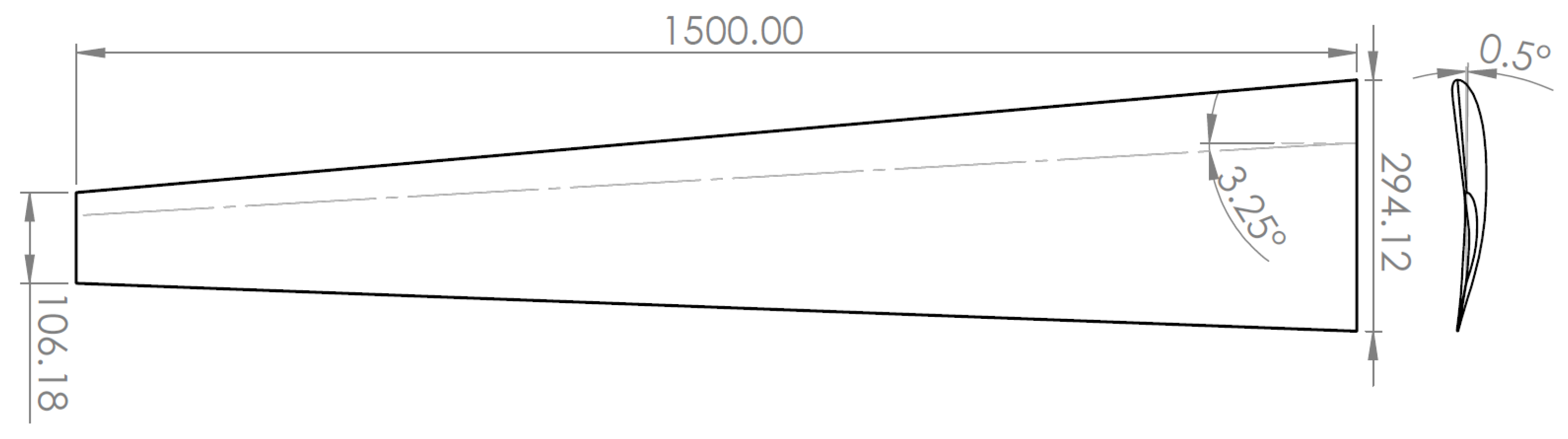
Based on the selected W/S value, the methodology determines the geometric characteristics of the main wing, starting with a fundamental parameter—the surface area. Once the surface area is established, other key characteristics, such as wingspan, aspect ratio, and taper ratio, are calculated, ultimately defining the complete wing geometry.
2.3. High-Fidelity CFD Aerodynamics
A numerical model of a wing, incorporating the average values of key geometric characteristics, was developed as the foundation for subsequent Computational Fluid Dynamics (CFD) analyses and optimization studies of various wing configurations derived from the surrogate model. The computational domain dimensions and boundary conditions were carefully designed to reflect the UAV’s operational environment and altitude. Simulations were conducted using ANSYS Fluent [22], solving the Reynolds-Averaged Navier-Stokes (RANS) equations coupled with the Spalart-Allmaras turbulence model [23]. The Spalart-Allmaras turbulence model was selected for its reliability in capturing high-lift aerodynamic effects. The computational domain was defined as a rectangular region measuring 6.0 × 4.0 × 10.0 m. The RANS equations were discretized using the Finite Volume Method (FVM) under incompressible, steady-state flow assumptions with an appropriately refined mesh. To ensure accurate boundary layer resolution, a first cell wall distance of was achieved, with the initial layer height set to m. A mesh independence study was also conducted to verify that further refinement did not impact the results, ensuring an optimal balance between accuracy and computational efficiency. The computational domain, including dimensions, boundary conditions, and mesh details, is illustrated in Figure 1 and Figure 2.
Pressure and temperature values were set according to the UAV’s maximum operating altitude, with a predefined inlet velocity. The outlet boundary conditions were defined with a zero pressure gradient, while the turbulence intensity was set to 1%. A symmetry boundary condition was applied along the longitudinal plane, and the wing surfaces were modeled as free-slip walls. For all wing configurations, the AoA varied from to to extract the relevant aerodynamic coefficients. The convergence of the lift and drag coefficients, and , respectively, is illustrated in Figure 3.
2.4. Surrogate Modeling
The key steps in a typical SBO process, as outlined in Alexandrov et al. [24], include:
- Sampling the design space and evaluating the objective function along with any constraints.
- Constructing the surrogate model based on the sampled data.
- Searching the design space and refining the surrogate model using update (infill) criteria.
- Enhancing the model by incorporating newly added points and repeating the process.
The sampling stage is a crucial step in an SBO algorithm, as the surrogate model’s accuracy depends on the selection of initial design points. To ensure the model represents the design space effectively, the most influential points must be chosen to maximize the information available for surrogate construction. Given the often high-dimensional nature of design problems, exhaustive grid searches become computationally prohibitive. Instead, more efficient techniques, such as Latin Hypercube Sampling (LHS) [25], are commonly used. LHS is a robust statistical method that generates parameter samples from a multidimensional distribution while maintaining a well-distributed design space representation. The method involves an optimization problem aimed at maximizing the distance between sample points while ensuring each coordinate follows a predefined probability distribution. Once the sampling is completed, the next step is to construct the surrogate model, typically represented as a general function:
where w denotes model parameters, and represents the design variables. A key criterion for selecting a surrogate model is its ability to accurately capture the desired function’s characteristics while maintaining flexibility. Overly rigid models risk instability and overfitting. One widely used surrogate model in engineering applications is Kriging [26,27], which expresses function approximations as a linear combination of basis functions (kernels) that depend on the Euclidean distance between design points. For noise-free data, the Kriging approximation is given by:
where:
- is the number of basis functions,
- represents the center of the n-th basis function,
- is the kernel function, evaluated based on the distance between the prediction point and the corresponding center.
The kernel function is typically defined as:
where and are model parameters.
The Kriging model is constructed using the following steps:
- Formulating the correlation matrix based on training data points:
- Maximizing the Maximum Likelihood Estimator (MLE):where is the MLE estimate of the standard deviation. In this study, p is set to 2.
- Predicting values at new design points:
For Gaussian-based processes, the Mean Squared Error (MSE) estimation is given by:
A commonly used approach for improvement is the Expected Improvement (EI) function:
where and denote the cumulative distribution and probability density functions, respectively. As an additional step toward more realistic SBO frameworks, constraints should be incorporated into the surrogate model. The approach to constraint handling depends on the computational cost of evaluating the constraint function. Constraints can either be evaluated directly or modeled using surrogate techniques similar to those applied to the objective function, effectively creating a surrogate model for each constraint. When constraint evaluations are computationally inexpensive, conventional constraint optimization methods, in conjunction with the objective function surrogate model, guide the SBO framework toward both promising and feasible regions of the design space. However, if surrogate models are also employed for constraints, the expected improvement function from Equation (15) is modified into the constrained expected improvement function by introducing the probability of feasibility:
where F represents the feasibility measure of a constraint g, and denotes the variance of the constraint’s Kriging model. The probability of achieving an improvement over the current minimum function value while satisfying feasibility conditions is then determined by multiplying Equations (15) and (16):
To determine the next point for model refinement, a sub-optimization problem is solved:
The resulting point, , is then added in the current dataset, which is then re-trained. This process is typically repeated for a predefined number of iterations [27]. This ensures that the surrogate model is updated efficiently, balancing exploration and exploitation for improved optimization performance.
2.5. Multi-Fidelity SBO Framework
The 1st SBO framework (Figure 4) employs variable fidelity analysis tools and is conducted in three phases. Following the conceptual design calculations of wing surface area () and the assumption of the airfoil’s maximum lift coefficient (), the 1st phase of the SBO starts with the preliminary selection of a number of existing airfoils present in the literature, so that they satisfy the previous assumption (high lift suitable for low Reynolds numbers airfoils). The 1st phase SBO then introduces the CST parameterization method in order to obtain the optimal airfoil shape for each of the selected baseline airfoils. The objective of this SBO is to maximize the airfoil’s lift coefficient while maintaining optimal aerodynamic performance at low Reynolds numbers. Once the optimal one of each airfoil class is obtained, a comparative evaluation is performed across various Reynolds numbers ( 75000 – 700000) using low-fidelity aerodynamics (XFLR5 software) in order to find the optimal one. With the selection of the optimal airfoil, the 2nd phase of the 1st SBO framework is initiated. This phase utilizes an SBO framework, employing low-fidelity aerodynamics (panel method) to identify the optimal wing geometry for the specific aircraft. The optimization objective is to maximize the wing’s lift-to-drag ratio (), subject to the following constraints: minimum lift-to-drag ratio at zero AoA (), minimum lift curve slope () and minimum stall AoA (). Moreover, this SBO considers four key geometric variables, the aspect ratio (AR), the taper ratio (), the quarter-chord sweep angle () and the tip twist angle (). At the end of the 2nd phase, an optimal wing geometry is determined based on low-fidelity aerodynamics. Therefore, and in order to further refine the low-fidelity optimal solution, a 3rd phase SBO is proposed, coupled with high-fidelity aerodynamics by means of CFD. The geometric variables from the 2nd phase were adjusted based on the low-fidelity optimal wing, and an additional constraint (wing maximum lift coefficient ()) was introduced, while the objective and the other three constraints remain the same. The 3rd phase leads to the first optimal wing design for the specific aircraft.
The 2nd SBO framework (Figure 5) consists of two phases. The 1st phase is identical to that of the 1st SBO framework, where existing high lift airfoils suitable for low Reynolds numbers are selected and optimized using SBO coupled with the CST method and low-fidelity aerodynamics (XFOIL). The 2nd phase of the 2nd SBO framework employs SBO directly coupled with high-fidelity aerodynamics by means of CFD, in order to determine the optimal wing geometry for the specific aircraft. The optimization objective and the three constraints remain the same as the 2nd phase of the 1st SBO framework, with an additional constraint to the maximum lift coefficient (), similar to the 3rd phase of the 1st SBO framework. The final phase of the 2nd SBO framework results in the second optimal wing design for the specific aircraft.
The SBO framework, as illustrated in Figure 6, is common to the two frameworks and consists of two main stages: the sampling stage and the model updating stage. The process begins with the definition of the sampling size, followed by generating samples using the LHS method. Subsequently, the geometry and mesh of the geometry are generated and further analyzed via each computational tool. The objective and constraint functions are then obtained for each sample. Once the training stage is completed, the main SBO framework is initiated. The hyperparameters of the Kriging model representing the objective and constraint functions are determined. Next, the constrained expected improvement function (Equation (17)) is minimized using a sub-optimization routine, yielding a new point in the design space. The computational analysis is then performed for this new point, and the surrogate model is updated accordingly. This iterative process continues for a predefined number of infill points.
3. Results
3.1. Conceptual Design Study
Given the assumption that a high-lift airfoil will be used for the UAV’s main wing, several airfoils were selected for analysis, including DAE 31, Eppler 423, and NACA 6412. Furthermore, an SBO framework utilizing a NACA 4-digit airfoil generator was conducted to identify an optimum NACA airfoil under the selected operating conditions. The optimization process determined that the optimal airfoil in this study was the NACA 7313. These airfoils were chosen for their favorable performance at an average low Reynolds number of 500,000, which aligns with the UAV’s operating conditions. To further refine their performance, the selected airfoils were represented using CST parameters, allowing for shape optimization to enhance characteristics such as maximum lift coefficient (), stall AoA (), and other aerodynamic properties. The CST parameters for each airfoil, as obtained from OpenVSP, are presented in Table 2. The original airfoils along with those parametrized using CST are also illustrated in Figure 7.
3.2. Airfoil Optimization Study
For the airfoil optimization study, the SBO technique was employed in combination with the CST parameterization method and the XFOIL code. Upper (ub) and lower boundaries (lb) were defined for each CST parameter of the selected airfoils, as presented in Table 3 and Table 4. The airfoils were generated based on these CST parameters and subsequently analyzed using XFOIL at a Reynolds number of , with an AoA varying from to 20o and a Mach number of zero.
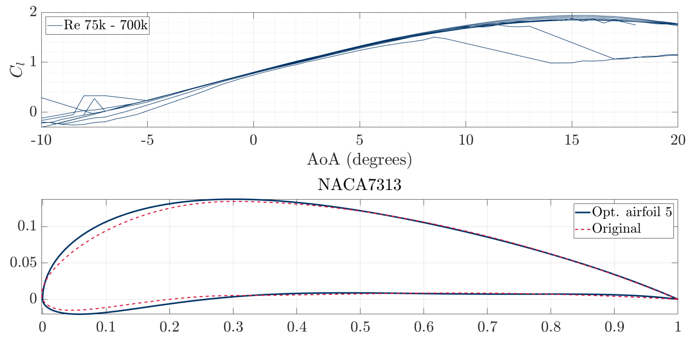
The objective of the SBO process was to maximize the lift-to-drag ratio (), with a constraint ensuring that the stall AoA was greater than 16o. The SBO sample size was set to 120 (), with 60 () infill points. Those values are suggested in Forrester et al. [28]. After completing the airfoil optimization, the best-performing airfoils, selected based on their maximum lift coefficient () and stall , were further analyzed across a Reynolds number range of to and an AoA from to 20o. However, optimized airfoils of NACA 6412 were excluded from further analysis, as none of the 180 generated airfoils in its SBO study achieved a maximum lift coefficient and stall AoA comparable to the other three airfoils. In the second phase of XFOIL analyses, the best-performing airfoils across the full Reynolds number range were selected from the SBO results of DAE-31 and NACA-7313. Optimized airfoils from the Eppler-423 SBO study were not chosen due to their poor performance at low Reynolds numbers ( – ). Figure 8, Figure 9 and Figure 10 illustrate the selected airfoils, along with XFOIL results for versus for each.
Figure 8.
Cl for various Reynolds numbers of DAE-31 (a) and NACA-7313 (b) airfoils.
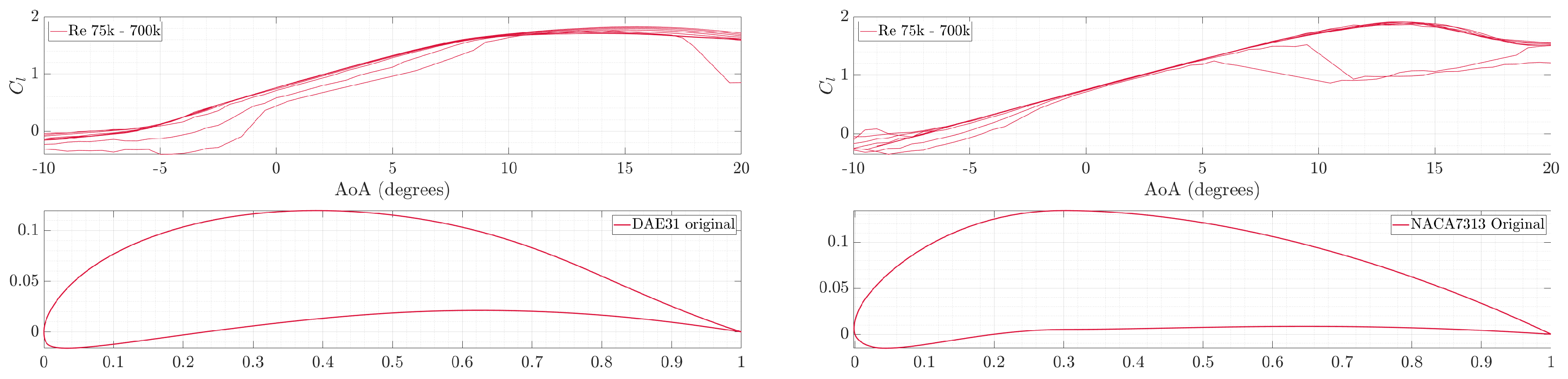
Figure 9.
Cl for various Reynolds numbers of 1st optimal airfoil selection (a) and 2nd optimal airfoil selection (b).
Figure 9.
Cl for various Reynolds numbers of 1st optimal airfoil selection (a) and 2nd optimal airfoil selection (b).
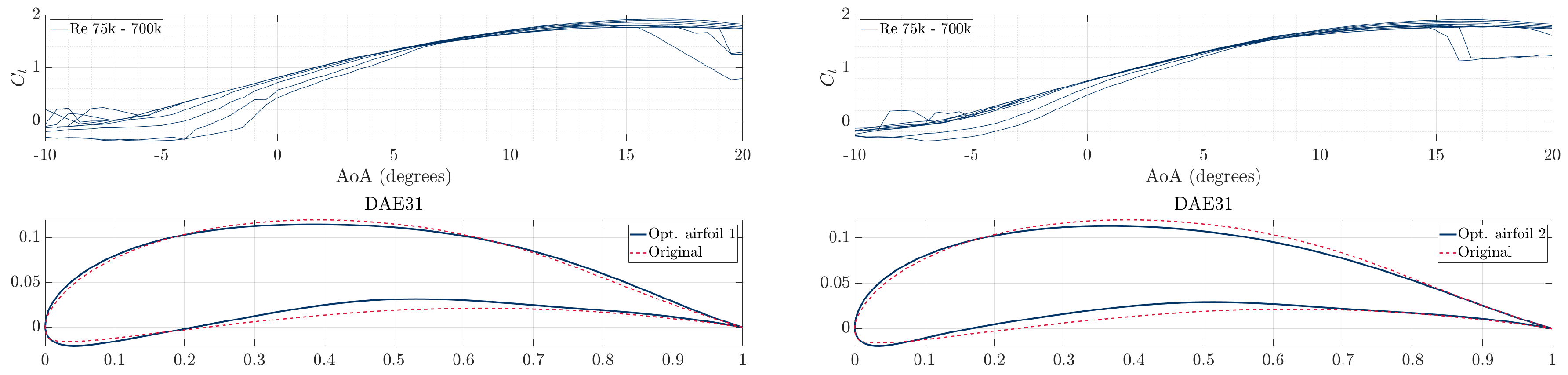
Figure 10.
Cl for various Reynolds numbers of 3rd optimal airfoil selection (a) and 4th optimal airfoil selection (b).
Figure 10.
Cl for various Reynolds numbers of 3rd optimal airfoil selection (a) and 4th optimal airfoil selection (b).
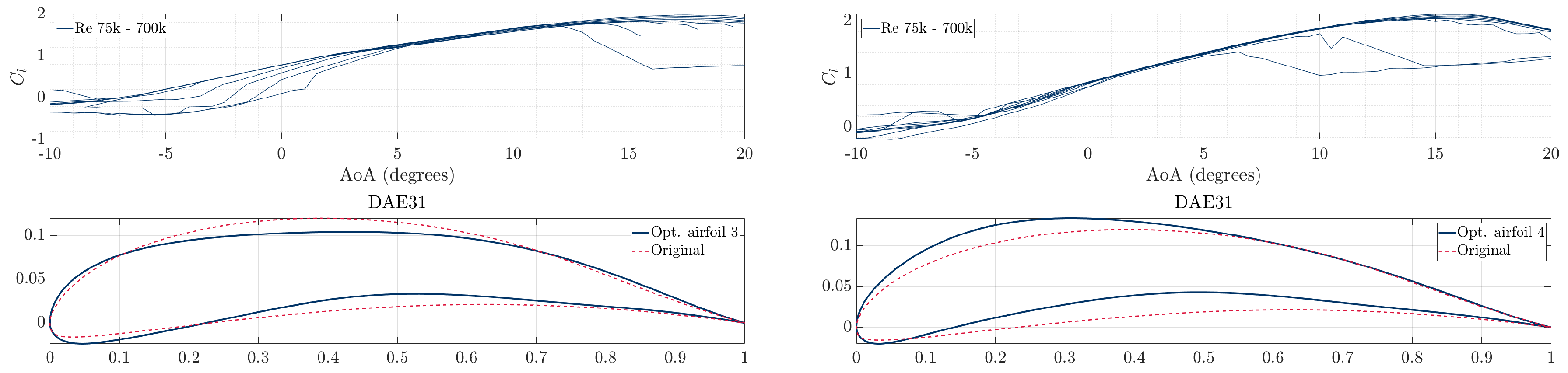
Figure 11.
Cl for various Reynolds numbers of 5th optimal airfoil selection.
3.3. Wing Optimization Study - Low-Fidelity Modules
In the second phase of the first SBO framework, an optimization study was conducted to determine the optimal wing geometry. Four geometric variables—aspect ratio (), taper ratio (), quarter-chord sweep angle ( ), and tip twist ()—were optimized within predefined lower and upper boundaries, as presented in Table 5. The wing reference area was kept constant throughout the study.
The aspect ratio varied between 6.5 and 15, corresponding to a UAV wingspan (b) of 2 to 3 meters, values typical for this UAV class. The taper ratio and quarter-chord sweep angle ranged from 0.2 to 1 and 0o to 30o, respectively, while tip twist varied between and 2o degrees. The objective of the SBO framework was to maximize the wing’s maximum lift-to-drag ratio (), with constraints ensuring a lift-to-drag ratio greater than 20 at 0o AoA, a stall AoA of at least 16o, and a lift curve slope exceeding 5.1 (). These constraints were applied to optimize aerodynamic performance by minimizing drag at low AoA (where the UAV operates for most of its flight envelope), increasing stall AoA to expand the operational envelope, and maximizing the lift curve slope to enhance lift response to small AoA changes, ensuring efficient climb and loiter phases.
The SBO study utilized 40 samples ( number of variables) with 20 infill points ( samples). To evaluate these 60 wing configurations, low-fidelity aerodynamic simulations were performed using XFLR5. This approach allowed for the analysis of all five selected airfoils within the SBO framework, as XFLR5 enabled rapid simulation of all 60 models (40 samples + 20 infill points). The panel method was employed for these simulations, with velocity and atmospheric conditions set according to the UAV’s operating envelope. Table 6 presents the geometric characteristics of the 20 infill points, while Table 7 lists their corresponding low-fidelity aerodynamic results, with the ones highlighted in red indicating the optimal wing (wing configuration 53). Results are provided for a single SBO case that best satisfies the three constraints. The 40 samples, along with the aerodynamic results presented in Appendix A in Table A1 and Table A2 respectively.
3.4. Wing Optimization Study—High-Fidelity Modules
3.4.1. 1st SBO Framework
The third phase of the first SBO framework (Figure 4) is coupled with high-fidelity aerodynamics to validate and refine the optimal wing characteristics obtained from the low-fidelity analysis in the second phase. To enhance the accuracy of the optimization while reducing computational costs, the boundaries of the geometric variables were adjusted based on the optimal wing geometry from the second phase, as listed in Table 8. For this phase, the aspect ratio was fixed at 15, as it provided the best aerodynamic performance in the previous phase. The boundary ranges for the remaining three geometric variables—taper ratio (), quarter-chord sweep angle (), and tip twist ()—were further narrowed to focus the optimization process on fine-tuning the wing shape.
Given that only three variables were considered, the total number of samples was reduced to 15, with 5 additional infill points. An additional constraint was introduced in this SBO phase, ensuring that the maximum lift coefficient () met the required performance criteria. This constraint was necessary because high-fidelity aerodynamics (using CFD) more accurately capture nonlinear aerodynamic effects, including stall onset and flow separation, which are not well represented in low-fidelity methods.
The final results show that the taper ratio () varies from 0.2 to 0.4, while the quarter-chord sweep angle () and tip twist () vary across the entire given range, and , respectively.
As shown in Table 10, none of the optimized wing models successfully met the constraints of the stall angle AoA () or the maximum lift coefficient (). This discrepancy is attributed to the significant separation of airflow across the wingspan at high AoA - an aerodynamic phenomenon that low-fidelity methods failed to accurately predict. The high camber of the selected airfoil exacerbates the flow separation, which starts to play a dominant role at AoA of about 12-13 degrees (Figure 12, leading to an earlier onset of stall than expected.
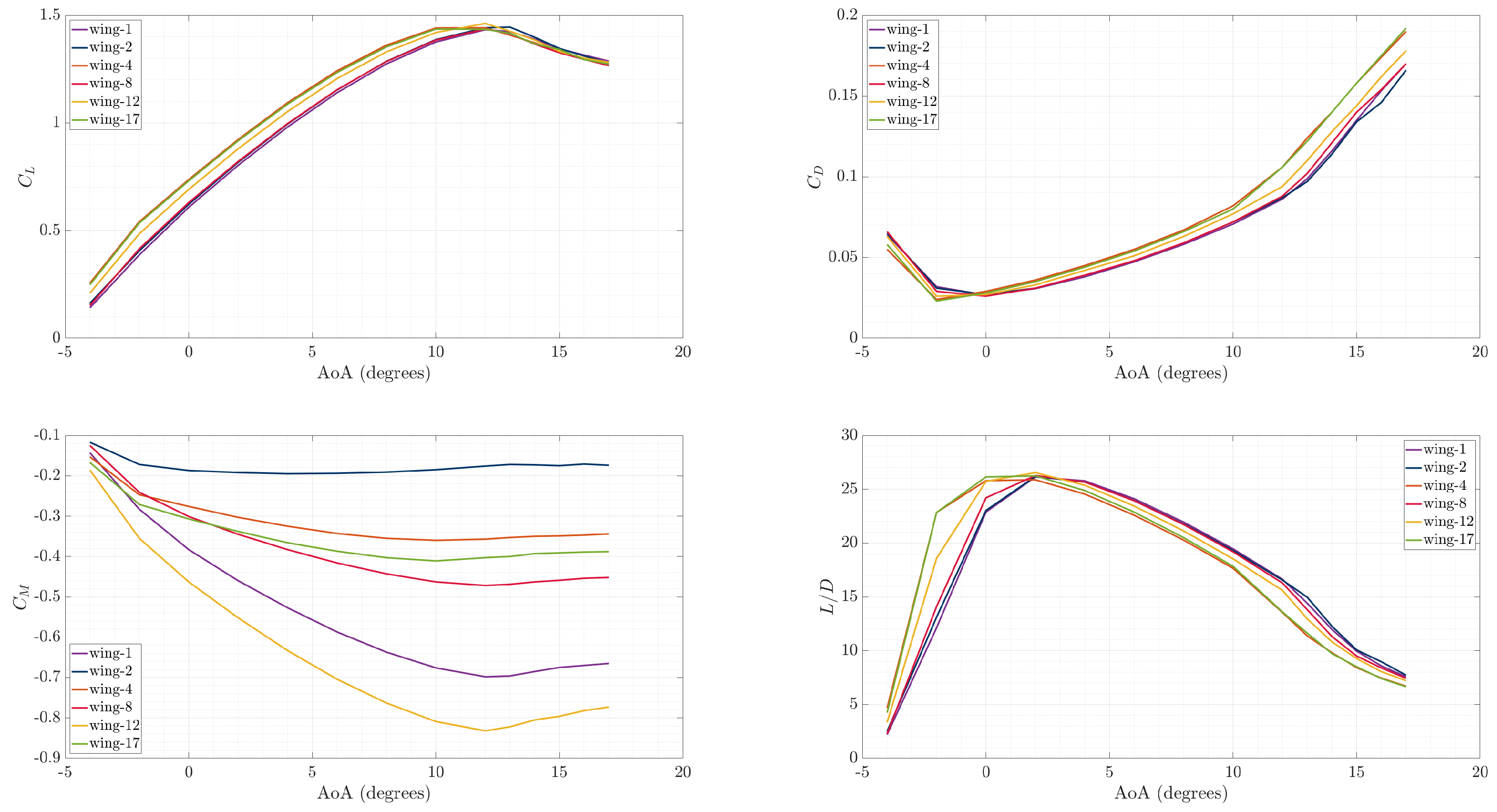
On the other hand, the other two constraints were successfully satisfied, with the slope of the lift curve () exceeding 5.65 1/rad and the lift-to-friction ratio at zero AoA () exceeding 22.5. The primary objective of this study - maximizing the lift-to-friction ratio - was achieved, with the best configuration (model 12) reaching a maximum L/D of 26.542. Figure 13 shows the aerodynamic results for the entire AoA range for the models with the best results of each coefficient of Table 10, which are highlighted with yellow, while Figure 14 presents the optimal wing geometry of the 1st SBO framework. The results of the optimal wing in Table 9 and Table 10 are highlighted in red (wing configuration 12).

Table 9.
Samples (1-15) and Infill points (16-20) of geometric characteristics - 3rd phase (SBO with CFD).
Table 9.
Samples (1-15) and Infill points (16-20) of geometric characteristics - 3rd phase (SBO with CFD).
| Wing conf. | b | ||||||
| 1 | 15 | 0.38 | 7.14 | -3.00 | 3.00 | 0.291 | 0.109 |
| 2 | 15 | 0.30 | 3.57 | -2.64 | 3.00 | 0.308 | 0.092 |
| 3 | 15 | 0.23 | 1.43 | 2.00 | 3.00 | 0.327 | 0.073 |
| 4 | 15 | 0.48 | 2.86 | 1.64 | 3.00 | 0.271 | 0.129 |
| 5 | 15 | 0.43 | 8.57 | -1.21 | 3.00 | 0.281 | 0.119 |
| 6 | 15 | 0.53 | 0.71 | -2.29 | 3.00 | 0.262 | 0.138 |
| 7 | 15 | 0.28 | 6.43 | -1.57 | 3.00 | 0.314 | 0.086 |
| 8 | 15 | 0.45 | 4.29 | -1.93 | 3.00 | 0.276 | 0.124 |
| 9 | 15 | 0.20 | 5.71 | 0.57 | 3.00 | 0.333 | 0.067 |
| 10 | 15 | 0.33 | 2.14 | -0.86 | 3.00 | 0.302 | 0.098 |
| 11 | 15 | 0.35 | 7.86 | 0.93 | 3.00 | 0.296 | 0.104 |
| 12 | 15 | 0.40 | 0.00 | 0.21 | 3.00 | 0.286 | 0.114 |
| 13 | 15 | 0.55 | 5.00 | - 0.14 | 3.00 | 0.258 | 0.142 |
| 14 | 15 | 0.50 | 9.29 | 1.29 | 3.00 | 0.267 | 0.133 |
| 15 | 15 | 0.25 | 10.00 | -0.50 | 3.00 | 0.320 | 0.080 |
| 16 | 15 | 0.22 | 0.00 | 0.66 | 3.00 | 0.327 | 0.073 |
| 17 | 15 | 0.31 | 3.59 | 2.00 | 3.00 | 0.305 | 0.095 |
| 18 | 15 | 0.20 | 10.00 | -2.63 | 3.00 | 0.333 | 0.067 |
| 19 | 15 | 0.20 | 6.89 | 2.00 | 3.00 | 0.333 | 0.067 |
| 20 | 15 | 0.40 | 3.91 | 0.33 | 3.00 | 0.286 | 0.114 |
Table 10.
High-fidelity aerodynamics results - 3rd phase (SBO with CFD).
| Wing conf. | |||||||
| 1 | 12 | 1.433 | 26.138 | 5.936 | 0.608 | 0.0266 | 22.879 |
| 2 | 13 | 1.445 | 26.191 | 5.936 | 0.622 | 0.0270 | 23.026 |
| 3 | 12 | 1.451 | 26.369 | 5.776 | 0.724 | 0.0278 | 26.019 |
| 4 | 12 | 1.442 | 25.874 | 5.776 | 0.737 | 0.0286 | 25.794 |
| 5 | 12 | 1.443 | 26.397 | 5.827 | 0.654 | 0.0262 | 24.968 |
| 6 | 12 | 1.434 | 25.970 | 5.896 | 0.609 | 0.0268 | 22.695 |
| 7 | 12 | 1.446 | 26.338 | 5.868 | 0.657 | 0.0266 | 24.726 |
| 8 | 12 | 1.436 | 26.271 | 5.856 | 0.630 | 0.0260 | 24.205 |
| 9 | 12 | 1.425 | 26.490 | 5.873 | 0.694 | 0.0270 | 25.756 |
| 10 | 12 | 1.460 | 26.366 | 5.839 | 0.668 | 0.0267 | 25.052 |
| 11 | 12 | 1.431 | 26.316 | 5.753 | 0.709 | 0.0273 | 25.967 |
| 12 | 12 | 1.462 | 26.542 | 5.827 | 0.691 | 0.0269 | 25.734 |
| 13 | 12 | 1.444 | 26.092 | 5.793 | 0.680 | 0.0268 | 25.399 |
| 14 | 12 | 1.431 | 25.818 | 5.741 | 0.722 | 0.0282 | 25.632 |
| 15 | 12 | 1.430 | 26.450 | 5.747 | 0.676 | 0.0265 | 25.564 |
| 16 | 12 | 1.438 | 26.216 | 5.713 | 0.691 | 0.0270 | 25.642 |
| 17 | 12 | 1.436 | 26.240 | 5.747 | 0.731 | 0.0280 | 26.142 |
| 18 | 12 | 1.429 | 26.208 | 5.827 | 0.644 | 0.0266 | 24.241 |
| 19 | 12 | 1.424 | 26.260 | 5.690 | 0.717 | 0.0275 | 26.093 |
| 20 | 12 | 1.441 | 26.331 | 5.799 | 0.697 | 0.0270 | 25.806 |
Figure 14.
Phase 3 contours for pressure coefficient (a), temperature (b), and velocity pathlines (c) of wing 12 at 12o .
Figure 14.
Phase 3 contours for pressure coefficient (a), temperature (b), and velocity pathlines (c) of wing 12 at 12o .
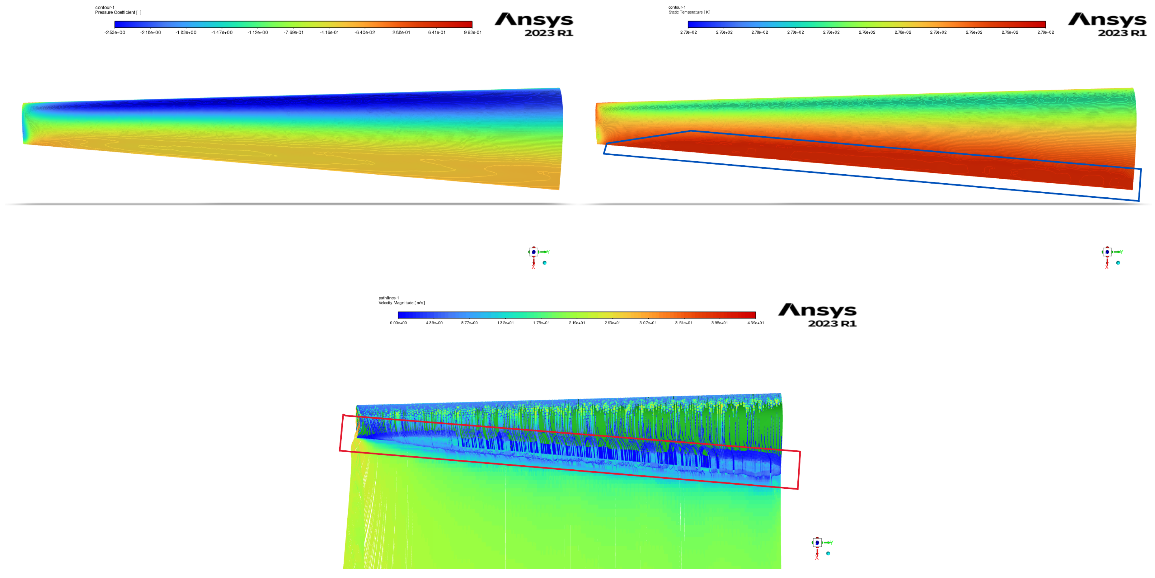
Figure 15.
Phase 3 results for (a), (b), (c) and (d) versous .
3.4.2. 2nd SBO Framework
In the second SBO framework (Figure 5), high-fidelity CFD aerodynamics are applied following the airfoil optimization phase (1st phase of the second SBO framework). The same 40 samples, as presented in Table A3 of Appendix A, are considered again as those of the 2nd phase of the first SBO framework (Figure 3), with lower and upper boundaries of the geometric variables remaining unchanged (Table 4). Moreover, an additional constraint was applied in this SBO, ensuring the maximum lift coefficient () meets the required performance criteria as in the third phase of the 1st SBO framework. The objective function, which aims to maximize the lift-to-drag ratio (L/D) and the other three existing constraints (, and ) remained the same. Twenty (20) infill points were then retrieved from the SBO, with their geometric characteristic and corresponding aerodynamic results summarized in Table 11 and Table 12.
The final variables of the 20 infill points from the second SBO framework (Table 11) indicate clear trends in the optimized wing geometries. The aspect ratio (AR) reached its upper boundary (15) in 16 out of the 20 cases. The taper ratio () varied across its entire range (), but most optimized values clustered near the lower boundary. For the quarter-chord sweep angle (), the maximum observed value was , with most optimized designs favoring minimal sweep (equal to zero), while the tip twist () varied throughout its allowable range ( – 2o).
The aerodynamic results from the 20 infill points of the second SBO framework (Table 12) indicate that only three models met the stall AoA constraint (), while the remaining 17 stalled at 14o - 15o. Similar to the findings in the third phase of the 1st SBO framework, none of the models satisfied the constraint. This limitation stems from significant airflow separation occurring at higher AoA, leading to a drop in lift across the wingspan.
On the other hand, the other two constraints—lift curve slope ( 1/rad) and lift-to-drag ratio at zero AoA ()—were successfully met. Additionally, the optimization objective of maximizing L/D was achieved, with the best-performing configuration (model 46) reaching a maximum lift-to-drag ratio of 26.845. The aerodynamic results for the entire AoA range of the 4 best-performing models are presented in Figure 16. Figure 17 presents the optimal wing geometry of the second SBO framework, with its geometrical characteristics and aerodynamics results highlighted in red in Table 11 and Table 12.
Figure 16.
Optimal wing configuration of 3rd phase of the 1st SBO.
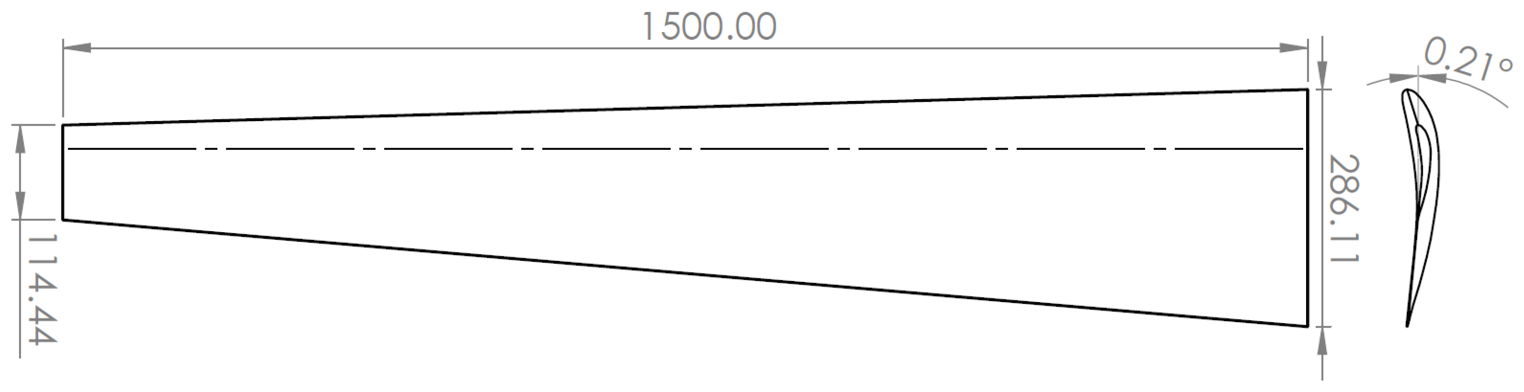
Figure 17.
Phase 2 of 2nd SBO framework contours for pressure coefficient (a), temperature (b), and velocity pathlines (c) of wing 46 at 14o .
Figure 17.
Phase 2 of 2nd SBO framework contours for pressure coefficient (a), temperature (b), and velocity pathlines (c) of wing 46 at 14o .
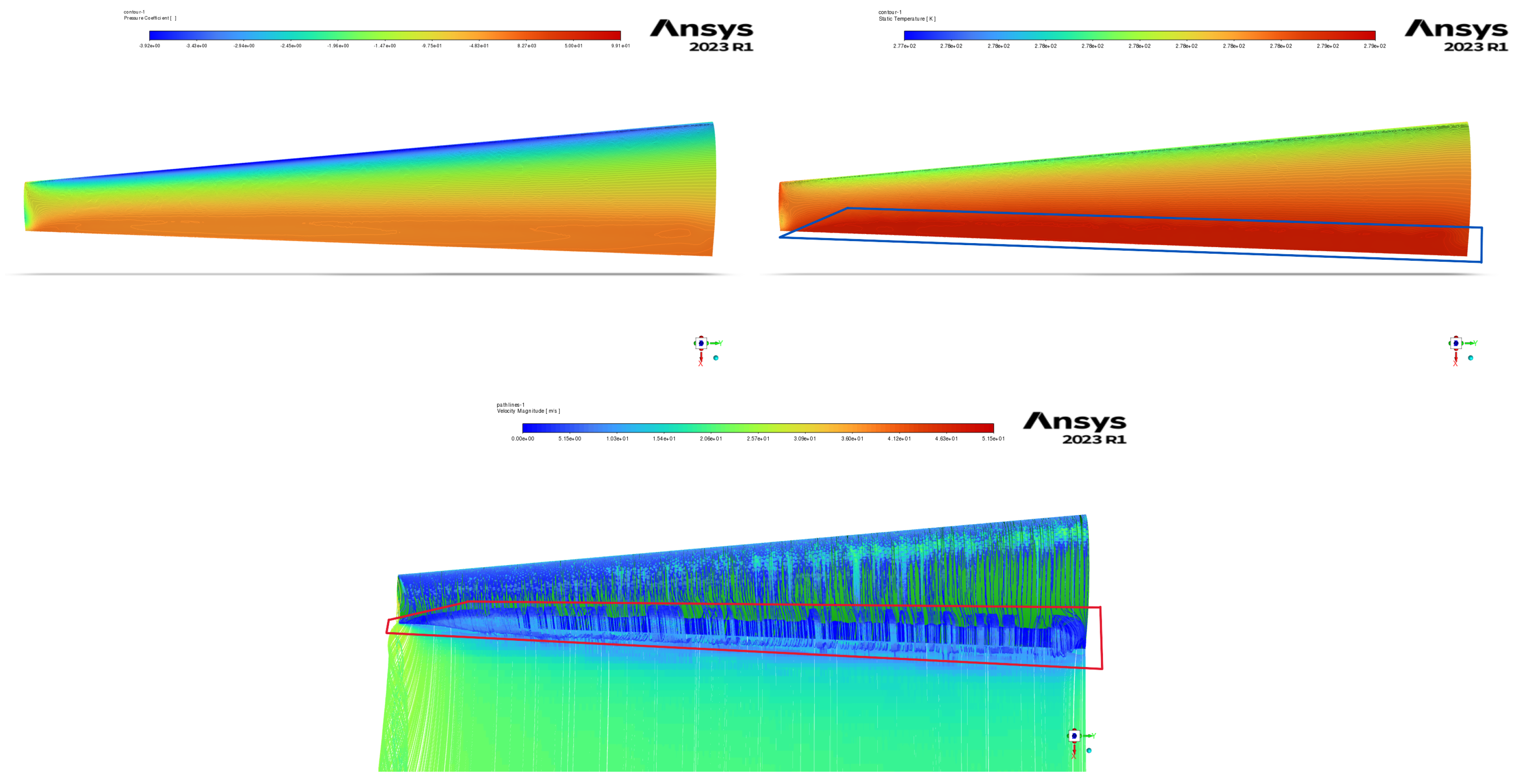
Figure 18.
2nd phase (SBO with CFD) results for (a), (b), (c) and (d) versus .
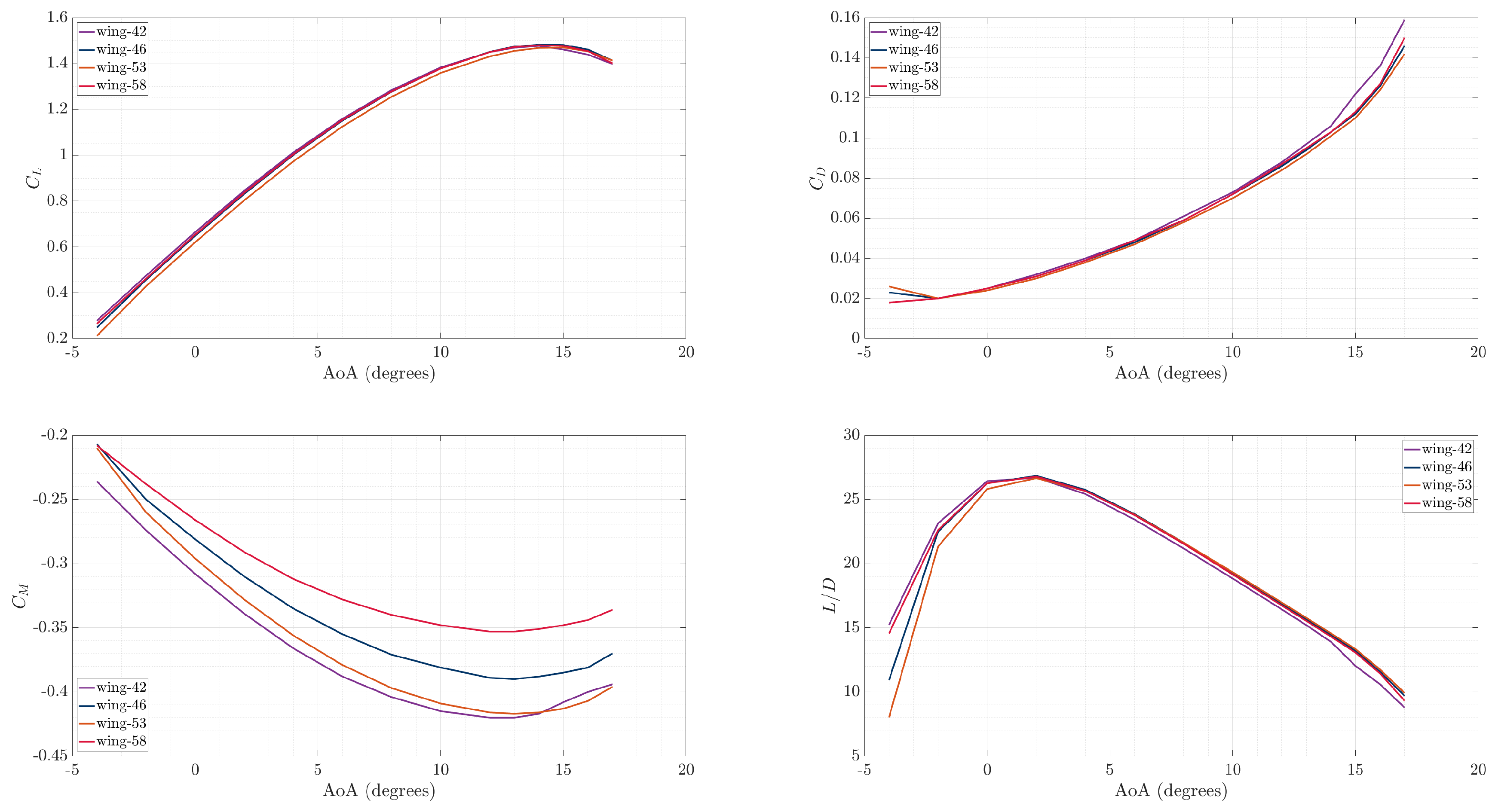
Figure 19.
Optimal wing configuration of 2nd phase of the 2nd SBO.
3.5. SBO Frameworks Optimal Wing Geometries Comparison
The final content of this study involves the comparison of the optimal wing form both SBO frameworks. Figure 20 illustrates the aerodynamic results of both optimal wings for various AoA, while Figure 21 presents their geometrical characteristics. As can be seen, the optimal 2nd SBO framework optimal wing exhibits maximum lift coefficient and stalls 2 degrees later than the first one. The drag coefficient of the 2nd optimal wing remains consistently lower across the entire AoA range, resulting higher lift-to-drag ratio, which was the primary objective of this study. The pitching moment coefficient derivative of both optimal wings, is negative until their respective stall angles, with the 2nd optimal wing’s curve being gentler in the change of the slope, which indicates smoother stall behavior. The aspect ratio of both optimal wings is 15, while for the other three geometric characteristics (taper ratio () and tip twist ()) are slightly different. The quarter-chord sweep angle () has a difference of 3 degrees. The main geometric difference between the optimal wings is the airfoil of each other, concluding that this is the main reason for the difference in the performance of each wing. The 1st optimal wing’s airfoil has greater camber, leading to higher lift curve slope (), which contributes to its earlier stall.
4. Discussion and Conclusions
In this study, a multi-fidelity surrogate-assisted aerodynamic optimization framework of aircraft wings was developed and applied in the conceptual design phase of a Class I mini-UAV. The methodology begins with the determination of the primary wing performance and geometric parameters, incorporating an assumed airfoil maximum lift coefficient and constraint diagram extraction. Subsequently, a multi-fidelity surrogate-based optimization (SBO) was implemented coupled with Class-Shape Transformation (CST) method, forming two distinct SBO frameworks. The first one, consists of three phases – SBO coupled with CST and XFOIL for low-fidelity aerodynamics to optimize the airfoil for the first phase, SBO coupled with XFLR5 for low-fidelity aerodynamics to generate an optimal wing geometry for the second phase, and for the third phase SBO coupled with high-fidelity aerodynamics by means of CFD is conducted, in order to refine the optimal wing geometry from phase two. For the second SBO framework, two phases were conducted. The first phase was identical to the first phase of the first SBO framework, while the second phase SBO coupled with high-fidelity aerodynamics is conducted right after the airfoil optimization, bypassing low-fidelity aerodynamics by means of the panel method. Both SBO frameworks produced similar wing geometric characteristics, but the aerodynamic and performance results varied due to differences in airfoil selection. The first SBO framework examined six airfoils in 2nd phase due to the efficiency of low-fidelity aerodynamics (panel method), allowing multiple simulations in a short time, and then the optimal wing geometry (Figure 12) was further optimized with SBO coupled with high-fidelity aerodynamics (phase 3), while the second phase of the second SBO framework analyzed one airfoil due to the higher computational cost of high-fidelity aerodynamics. The second phase of the first SBO framework identified optimal airfoil 4 (Figure 13), which exceeded the aerodynamic constraints in most of the 40 samples and 20 infill points. However, in the third phase, the optimal wing geometry didn’t meet the stall angle of attack and maximum lift coefficient constraints, revealing that low-fidelity aerodynamics can not capture nonlinear aerodynamic effects at high angles of attack, like flow separation and stall phenomena. In contrast, in the second phase of the second SBO framework, a different airfoil was used (optimal airfoil 1 – Figure 9a), chosen for its better performance at low Reynolds number, despite having a lower maximum lift coefficient than optimal airfoil 4. This resulted in better aerodynamic performance for the optimal wing geometry as depicted in Section 3.5. Moreover, both SBO frameworks successfully achieved the primary objective of this study, demonstrating the effectiveness of multi-fidelity surrogate-assisted aerodynamic optimization of aircraft wings. The results highlight that combining low- and high-fidelity models coupled with SBO techniques can significantly improve optimization efficiency, reducing computational costs while maintaining high accuracy in aerodynamic performance predictions. In addition, in the wing conceptual design process, the selection of the airfoil plays a critical role in determining overall aerodynamic performance. The second framework, which bypassed the low-fidelity aerodynamics (phase 2 of the first SBO framework) and relied directly on high-fidelity aerodynamics, identified a higher performance wing, reinforcing the importance of accurate modeling of nonlinear aerodynamic phenomena during the optimization process.
Finally, several improvements can be incorporated in both SBO frameworks presented in this paper in order to obtain more comprehensive aerodynamic design and optimization methodologies. The present methodology could benefit by automating the overall conceptual and preliminary design stages for the entire aircraft configuration, leveraging multi-fidelity optimization techniques. Coupling aerodynamic optimization with structural analysis to evaluate aeroelastic effects, such as flutter and structural deformation, could also enhance the efficiency of the present framework. Also, expanding the optimization process to consider multidisciplinary constraints, including weight optimization and stability analyses, could evolve into a more holistic approach for the aerodynamic optimization of UAVs and other aircraft configurations.
Author Contributions
Conceptualization, E.N. and S.K.; methodology, E.N. and S.K.; software, E.N. and S.K.; validation, E.N. and S.K.; formal analysis, E.N. and S.K.; investigation, E.N. and S.K.; resources, E.N. and S.K.; data curation, E.N. and S.K.; writing—original draft preparation, E.N. and S.K.; writing—review and editing, E.N. and S.K.; visualization, E.N. and S.K.; supervision, S.K. and V.K.; project administration, E.N. and S.K. and V.K. All authors have read and agreed to the published version of the manuscript.
Funding
This research received no external funding.
Institutional Review Board Statement
Not applicable.
Informed Consent Statement
Not applicable.
Data Availability Statement
Data are available on request.
Conflicts of Interest
The authors declare no conflict of interest.
Abbreviations
The following abbreviations are used in this manuscript:
| Angle of Attack | |
| Above Sea Level | |
| Computational Fluid Dynamics | |
| Finite Volume Method | |
| Mean Aerodynamic Chord | |
| Mean Squared Error | |
| Reynolds Averaged Navier Stokes | |
| Surrogate Based Optimization | |
| Sea Level | |
| Unmanned Aerial Vehicle |
Appendix A Appendix
Appendix A.1. Low- and High-Fidelity Results of SBO Samples
Table A1.
Samples of both Low- and High-Fidelity SBO - 2nd phase SBO of both methodologies.
| Wing conf. | |||||||
| 1 | 9.55 | 0.59 | 8.46 | 1.23 | 2.39 | 0.315 | 0.186 |
| 2 | 8.24 | 0.49 | 16.92 | -3.54 | 2.22 | 0.362 | 0.177 |
| 3 | 7.59 | 0.28 | 12.31 | 0.92 | 2.13 | 0.439 | 0.123 |
| 4 | 9.99 | 0.94 | 13.85 | 0.00 | 2.45 | 0.253 | 0.237 |
| 5 | 11.73 | 0.75 | 7.69 | 0.77 | 2.65 | 0.258 | 0.194 |
| 6 | 11.51 | 0.45 | 3.08 | 1.69 | 2.63 | 0.315 | 0.142 |
| 7 | 12.17 | 0.90 | 23.08 | -2.00 | 2.70 | 0.234 | 0.210 |
| 8 | 11.95 | 0.84 | 28.46 | 1.85 | 2.68 | 0.244 | 0.205 |
| 9 | 14.35 | 0.77 | 18.46 | -0.77 | 2.93 | 0.231 | 0.178 |
| 10 | 13.26 | 0.53 | 5.38 | -2.46 | 2.82 | 0.278 | 0.147 |
| 11 | 11.08 | 0.34 | 4.62 | -1.69 | 2.58 | 0.347 | 0.118 |
| 12 | 12.82 | 0.69 | 10.77 | -3.69 | 2.77 | 0.256 | 0.177 |
| 13 | 12.60 | 0.26 | 21.54 | 1.38 | 2.75 | 0.346 | 0.090 |
| 14 | 9.77 | 1.00 | 17.69 | -2.77 | 2.42 | 0.248 | 0.248 |
| 15 | 10.42 | 0.96 | 6.15 | -2.62 | 2.50 | 0.245 | 0.235 |
| 16 | 14.13 | 0.20 | 16.15 | 1.08 | 2.91 | 0.343 | 0.069 |
| 17 | 15.00 | 0.30 | 20.77 | -2.31 | 3.00 | 0.308 | 0.092 |
| 18 | 13.47 | 0.36 | 26.15 | -3.23 | 2.84 | 0.310 | 0.112 |
| 19 | 7.37 | 0.57 | 13.08 | 2.00 | 2.10 | 0.363 | 0.207 |
| 20 | 6.94 | 0.41 | 27.69 | -1.23 | 2.04 | 0.417 | 0.171 |
| 21 | 7.15 | 0.67 | 1.54 | -1.38 | 2.07 | 0.347 | 0.232 |
| 22 | 9.12 | 0.61 | 6.92 | -3.85 | 2.34 | 0.319 | 0.194 |
| 23 | 12.38 | 0.38 | 26.92 | 0.15 | 2.73 | 0.319 | 0.121 |
| 24 | 11.29 | 0.63 | 20.00 | -1.08 | 2.60 | 0.283 | 0.178 |
| 25 | 8.68 | 0.71 | 15.38 | 0.62 | 2.28 | 0.308 | 0.218 |
| 26 | 13.04 | 0.24 | 10.00 | -0.46 | 2.80 | 0.346 | 0.083 |
| 27 | 10.21 | 0.43 | 22.31 | -1.54 | 2.48 | 0.339 | 0.146 |
| 28 | 6.72 | 0.51 | 2.31 | -3.38 | 2.01 | 0.396 | 0.202 |
| 29 | 8.03 | 0.92 | 25.38 | 1.54 | 2.19 | 0.285 | 0.262 |
| 30 | 8.90 | 0.55 | 29.23 | -0.31 | 2.31 | 0.335 | 0.184 |
| 31 | 6.50 | 0.65 | 19.23 | -1.85 | 1.97 | 0.368 | 0.239 |
| 32 | 8.46 | 0.32 | 24.62 | -4.00 | 2.25 | 0.404 | 0.129 |
| 33 | 14.78 | 0.73 | 30.00 | -2.15 | 2.98 | 0.233 | 0.170 |
| 34 | 7.81 | 0.88 | 0.00 | -2.92 | 2.16 | 0.295 | 0.259 |
| 35 | 10.64 | 0.86 | 23.85 | -0.62 | 2.53 | 0.255 | 0.220 |
| 36 | 9.33 | 0.22 | 11.54 | -0.92 | 2.37 | 0.416 | 0.091 |
| 37 | 14.56 | 0.82 | 9.23 | -0.15 | 2.96 | 0.223 | 0.183 |
| 38 | 13.69 | 0.47 | 0.77 | 0.31 | 2.87 | 0.285 | 0.134 |
| 39 | 13.91 | 0.98 | 3.85 | 0.46 | 2.89 | 0.210 | 0.206 |
| 40 | 10.86 | 0.79 | 14.62 | -3.08 | 2.55 | 0.263 | 0.207 |
Table A2.
Results of Low-Fidelity SBO Samples.
| Wing conf. | |||||||
| 1 | 13 | 1.738 | 22.991 | 4.921 | 0.644 | 0.0287 | 22.413 |
| 2 | 16 | 1.765 | 21.665 | 4.707 | 0.493 | 0.0259 | 19.014 |
| 3 | 13 | 1.631 | 21.120 | 4.656 | 0.598 | 0.0286 | 20.883 |
| 4 | 14 | 1.740 | 22.689 | 4.817 | 0.590 | 0.0276 | 21.352 |
| 5 | 12.5 | 1.749 | 24.798 | 5.108 | 0.652 | 0.0280 | 23.275 |
| 6 | 12 | 1.750 | 25.262 | 5.184 | 0.680 | 0.0281 | 24.179 |
| 7 | 15 | 1.754 | 24.796 | 4.849 | 0.516 | 0.0262 | 19.722 |
| 8 | 15 | 1.758 | 21.978 | 4.507 | 0.612 | 0.0263 | 23.301 |
| 9 | 13 | 1.743 | 27.000 | 5.140 | 0.596 | 0.0266 | 22.421 |
| 10 | 13 | 1.762 | 27.040 | 5.332 | 0.573 | 0.0263 | 21.798 |
| 11 | 13 | 1.746 | 24.876 | 5.174 | 0.593 | 0.0264 | 22.485 |
| 12 | 14 | 1.755 | 26.481 | 5.213 | 0.507 | 0.0265 | 19.136 |
| 13 | 11 | 1.617 | 26.721 | 5.089 | 0.650 | 0.0265 | 24.500 |
| 14 | 15.5 | 1.715 | 22.793 | 4.724 | 0.474 | 0.0253 | 18.724 |
| 15 | 13.5 | 1.647 | 23.815 | 4.949 | 0.504 | 0.0257 | 19.639 |
| 16 | 10 | 1.583 | 28.343 | 5.294 | 0.665 | 0.0262 | 25.341 |
| 17 | 12.5 | 1.724 | 28.933 | 5.257 | 0.594 | 0.0257 | 23.143 |
| 18 | 14 | 1.743 | 27.309 | 5.015 | 0.542 | 0.0257 | 21.089 |
| 19 | 14.5 | 1.744 | 20.243 | 4.564 | 0.623 | 0.0309 | 20.182 |
| 20 | 16 | 1.681 | 19.978 | 4.323 | 0.517 | 0.0269 | 19.186 |
| 21 | 16 | 1.752 | 20.233 | 4.558 | 0.525 | 0.0271 | 19.354 |
| 22 | 15 | 1.734 | 22.572 | 4.900 | 0.486 | 0.0262 | 18.544 |
| 23 | 12.5 | 1.660 | 26.065 | 4.913 | 0.605 | 0.0262 | 23.091 |
| 24 | 14 | 1.752 | 24.567 | 4.943 | 0.571 | 0.0263 | 21.677 |
| 25 | 14 | 1.722 | 21.593 | 4.708 | 0.600 | 0.0286 | 20.999 |
| 26 | 11.5 | 1.693 | 27.007 | 5.309 | 0.640 | 0.0262 | 24.398 |
| 27 | 14 | 1.722 | 23.900 | 4.859 | 0.561 | 0.0261 | 21.500 |
| 28 | 17.5 | 1.792 | 19.517 | 4.510 | 0.474 | 0.0267 | 17.789 |
| 29 | 15.5 | 1.722 | 19.773 | 4.353 | 0.584 | 0.0301 | 19.417 |
| 30 | 15.5 | 1.727 | 21.867 | 4.502 | 0.546 | 0.0268 | 20.348 |
| 31 | 18 | 1.783 | 19.286 | 4.323 | 0.490 | 0.0266 | 18.408 |
| 32 | 15 | 1.682 | 21.946 | 4.635 | 0.502 | 0.0258 | 19.438 |
| 33 | 15.5 | 1.789 | 27.224 | 4.834 | 0.514 | 0.0265 | 19.428 |
| 34 | 15 | 1.650 | 20.996 | 4.632 | 0.471 | 0.0256 | 18.405 |
| 35 | 15 | 1.752 | 23.120 | 4.711 | 0.552 | 0.0268 | 20.615 |
| 36 | 12 | 1.612 | 23.108 | 4.932 | 0.595 | 0.0269 | 22.096 |
| 37 | 12 | 1.730 | 27.354 | 5.288 | 0.637 | 0.0270 | 23.581 |
| 38 | 12 | 1.770 | 27.483 | 5.366 | 0.661 | 0.0269 | 24.590 |
| 39 | 11.5 | 1.693 | 26.460 | 5.226 | 0.657 | 0.0276 | 23.764 |
| 40 | 14.5 | 1.725 | 24.282 | 4.961 | 0.498 | 0.0259 | 19.245 |
Table A3.
Results of High-Fidelity SBO Samples.
| Wing conf. | |||||||
| 1 | 15 | 1.463 | 21.880 | 5.289 | 0.630 | 0.0288 | 21.880 |
| 2 | 17 | 1.375 | 21.166 | 5.054 | 0.483 | 0.0238 | 20.313 |
| 3 | 16 | 1.437 | 20.362 | 4.956 | 0.587 | 0.0288 | 20.362 |
| 4 | 15 | 1.393 | 21.400 | 5.151 | 0.576 | 0.0269 | 21.400 |
| 5 | 14 | 1.453 | 23.357 | 5.380 | 0.632 | 0.0271 | 23.357 |
| 6 | 15 | 1.488 | 23.938 | 5.461 | 0.661 | 0.0276 | 23.938 |
| 7 | 15 | 1.268 | 23.553 | 5.002 | 0.489 | 0.0222 | 22.061 |
| 8 | 14 | 1.224 | 21.803 | 4.618 | 0.593 | 0.0272 | 21.803 |
| 9 | 15 | 1.351 | 25.517 | 5.306 | 0.567 | 0.0234 | 24.245 |
| 10 | 16 | 1.445 | 25.607 | 5.552 | 0.550 | 0.0228 | 24.074 |
| 11 | 16 | 1.459 | 23.780 | 5.409 | 0.573 | 0.0246 | 23.265 |
| 12 | 16 | 1.396 | 24.984 | 5.444 | 0.485 | 0.0215 | 22.548 |
| 13 | 14 | 1.375 | 25.164 | 5.231 | 0.625 | 0.0252 | 24.846 |
| 14 | 16 | 1.310 | 21.822 | 5.008 | 0.457 | 0.0224 | 20.404 |
| 15 | 16 | 1.397 | 22.690 | 5.249 | 0.488 | 0.0229 | 21.317 |
| 16 | 14 | 1.422 | 26.238 | 5.380 | 0.638 | 0.0246 | 25.897 |
| 17 | 15 | 1.364 | 26.877 | 5.375 | 0.567 | 0.0224 | 25.341 |
| 18 | 15 | 1.275 | 25.678 | 5.123 | 0.514 | 0.0216 | 23.849 |
| 19 | 12 | 1.424 | 26.260 | 5.690 | 0.717 | 0.0275 | 26.093 |
| 20 | 17 | 1.305 | 19.462 | 4.647 | 0.509 | 0.0262 | 19.462 |
| 21 | 17 | 1.431 | 19.351 | 4.945 | 0.516 | 0.0267 | 19.349 |
| 22 | 17 | 1.412 | 21.855 | 5.226 | 0.472 | 0.0230 | 20.510 |
| 23 | 14 | 1.290 | 24.800 | 5.025 | 0.578 | 0.0240 | 24.102 |
| 24 | 15 | 1.349 | 23.504 | 5.174 | 0.550 | 0.0240 | 22.891 |
| 25 | 15 | 1.405 | 20.681 | 5.071 | 0.591 | 0.0286 | 20.681 |
| 26 | 15 | 1.465 | 25.665 | 5.518 | 0.618 | 0.0247 | 25.014 |
| 27 | 15 | 1.349 | 23.012 | 5.117 | 0.546 | 0.0242 | 22.558 |
| 28 | 17 | 1.414 | 18.909 | 4.848 | 0.464 | 0.0250 | 18.535 |
| 29 | 16 | 1.280 | 18.910 | 4.630 | 0.566 | 0.0299 | 18.910 |
| 30 | 15 | 1.246 | 21.190 | 4.739 | 0.527 | 0.0251 | 20.971 |
| 31 | 17 | 1.351 | 18.545 | 4.710 | 0.483 | 0.0261 | 18.536 |
| 32 | 17 | 1.324 | 21.359 | 4.928 | 0.490 | 0.0237 | 20.731 |
| 33 | 14 | 1.162 | 24.978 | 4.744 | 0.474 | 0.0208 | 22.798 |
| 34 | 17 | 1.389 | 20.152 | 4.974 | 0.459 | 0.0238 | 19.279 |
| 35 | 15 | 1.276 | 22.096 | 4.871 | 0.530 | 0.0245 | 21.624 |
| 36 | 15 | 1.444 | 22.106 | 5.191 | 0.581 | 0.0263 | 22.106 |
| 37 | 15 | 1.439 | 25.523 | 5.421 | 0.612 | 0.0247 | 24.810 |
| 38 | 14 | 1.480 | 25.795 | 5.575 | 0.637 | 0.0251 | 25.357 |
| 39 | 15 | 1.457 | 24.514 | 5.386 | 0.634 | 0.0262 | 24.230 |
| 40 | 16 | 1.364 | 23.284 | 5.237 | 0.480 | 0.0222 | 21.641 |
References
- Salunke, N.; Ahamad, J.; Channiwala, S. Airfoil Parameterization Techniques: A Review. American Journal of Mechanical Engineering 2014, 2, 99–102. [CrossRef]
- Khurana, M.; Winarto, H.; Sinha, A., Airfoil Optimisation by Swarm Algorithm with Mutation and Artificial Neural Networks. In 47th AIAA Aerospace Sciences Meeting including The New Horizons Forum and Aerospace Exposition. [CrossRef]
- Masters, D.A.; Taylor, N.J.; Rendall, T.C.S.; Allen, C.B.; Poole, D.J. Geometric Comparison of Aerofoil Shape Parameterization Methods. AIAA Journal 2017, 55, 1575–1589. [CrossRef]
- Vecchia, P.D.; Daniele, E.; Amato, E.D. An airfoil shape optimization technique coupling PARSEC parameterization and evolutionary algorithm. Aerospace Science and Technology 2014, 32, 103–110. [CrossRef]
- Anitha, D.; Shamili, G.; Ravi Kumar, P.; Sabari Vihar, R. Air foil Shape Optimization Using Cfd And Parametrization Methods. Materials Today: Proceedings 2018, 5, 5364–5373. [CrossRef]
- Karman, M.; McNamara, M.; Coder, J.G. Airfoil Optimization via the Class-Shape Transformation and Orthogonal Deformation Modes. In Proceedings of the AIAA Aviation 2019 Forum. American Institute of Aeronautics and Astronautics, 2019. [CrossRef]
- Akram, M.T.; Kim, M.H. Aerodynamic Shape Optimization of NREL S809 Airfoil for Wind Turbine Blades Using Reynolds-Averaged Navier Stokes Model—Part II. Applied Sciences 2021, 11. [CrossRef]
- Akram, M.T.; Kim, M.H. CFD Analysis and Shape Optimization of Airfoils Using Class Shape Transformation and Genetic Algorithm—Part I. Applied Sciences 2021, 11. [CrossRef]
- Belda, M.; Hyhlík, T. Interactive Airfoil Optimization Using Parsec Parametrization and Adjoint Method. Applied Sciences 2024, 14. [CrossRef]
- Rouco, P.; Orgeira-Crespo, P.; Rey González, G.D.; Aguado-Agelet, F. Airfoil Optimization and Analysis Using Global Sensitivity Analysis and Generative Design. Aerospace 2025, 12. [CrossRef]
- Lyu, Z.; Kenway, G.K.W.; Martins, J.R.R.A. Aerodynamic Shape Optimization Investigations of the Common Research Model Wing Benchmark. AIAA Journal 2015, 53, 968–985. [CrossRef]
- Chen, S.; Lyu, Z.; Kenway, G.K.W.; Martins, J.R.R.A. Aerodynamic Shape Optimization of Common Research Model Wing–Body–Tail Configuration. Journal of Aircraft 2016, 53, 276–293. [CrossRef]
- Benaouali, A.; Kachel, S. Multidisciplinary design optimization of aircraft wing using commercial software integration. Aerospace Science and Technology 2019, 92, 766–776. [CrossRef]
- Ghafoorian, F.; Wan, H.; Chegini, S. A Systematic Analysis of a Small-Scale HAWT Configuration and Aerodynamic Performance Optimization Through Kriging, Factorial, and RSM Methods. Journal of Applied and Computational Mechanics 2024, pp. –. [CrossRef]
- Zheng, B.; Moni, A.; Yao, W.; Xu, M. Manifold Learning for Aerodynamic Shape Design Optimization. Aerospace 2025, 12. [CrossRef]
- Nikolaou, E.; Kilimtzidis, S.; Kostopoulos, V. Winglet Design for Aerodynamic and Performance Optimization of UAVs via Surrogate Modeling. Aerospace 2025, 12, 36. [CrossRef]
- Kilimtzidis, S.; Kostopoulos, V. Static Aeroelastic Optimization of High-Aspect-Ratio Composite Aircraft Wings via Surrogate Modeling. Aerospace 2023, 10, 251. [CrossRef]
- Kontogiannis, S.G.; Savill, M.A. A generalized methodology for multidisciplinary design optimization using surrogate modelling and multifidelity analysis. Optimization and Engineering 2020, 21, 723–759. [CrossRef]
- Bordogna, M.T.; Bettebghor, D.; Blondeau, C.; de Breuker, R. Surrogate-based aerodynamics for composite wing box sizing. In Proceedings of the 17th International Forum on Aeroelasticity and Structural Dynamics, 2017.
- Raymer, D.P. Aircraft design: A conceptual approach, 6 ed.; AIAA Education Series, American Institute of Aeronautics & Astronautics: Reston, VA, 2018.
- Roskam, J.; Lan, C. Airplane Aerodynamics and Performance; Airplane design and analysis, Roskam Aviation and Engineering, 1997.
- Ansys, Inc., Canonsburg, PA. Ansys Fluent User’s Guide, 2023. Accessed: 2023-03-27.
- Spalart, P.; Allmaras, S. A one-equation turbulence model for aerodynamic flows. In Proceedings of the 30th Aerospace Sciences Meeting and Exhibit. American Institute of Aeronautics and Astronautics, 1992. [CrossRef]
- Alexandrov, N.M.; Dennis, J.E.; Lewis, R.M.; Torczon, V. A trust-region framework for managing the use of approximation models in optimization. Structural Optimization 1998, 15, 16–23. [CrossRef]
- McKay, M.D.; Beckman, R.J.; Conover, W.J. Comparison of Three Methods for Selecting Values of Input Variables in the Analysis of Output from a Computer Code. Technometrics 1979, 21, 239–245. [CrossRef]
- Jones, D.R. A Taxonomy of Global Optimization Methods Based on Response Surfaces. Journal of Global Optimization 2001, 21, 345–383. [CrossRef]
- Forrester, A.I.J.; Sóbester, A.; Keane, A.J. Engineering Design via Surrogate Modelling; Wiley, 2008. [CrossRef]
- Forrester, A.I.; Sóbester, A.; Keane, A.J. Multi-fidelity optimization via surrogate modelling. Proceedings of the Royal Society A: Mathematical, Physical and Engineering Sciences 2007, 463, 3251–3269. [CrossRef]
Figure 1.
CFD domain characteristics.
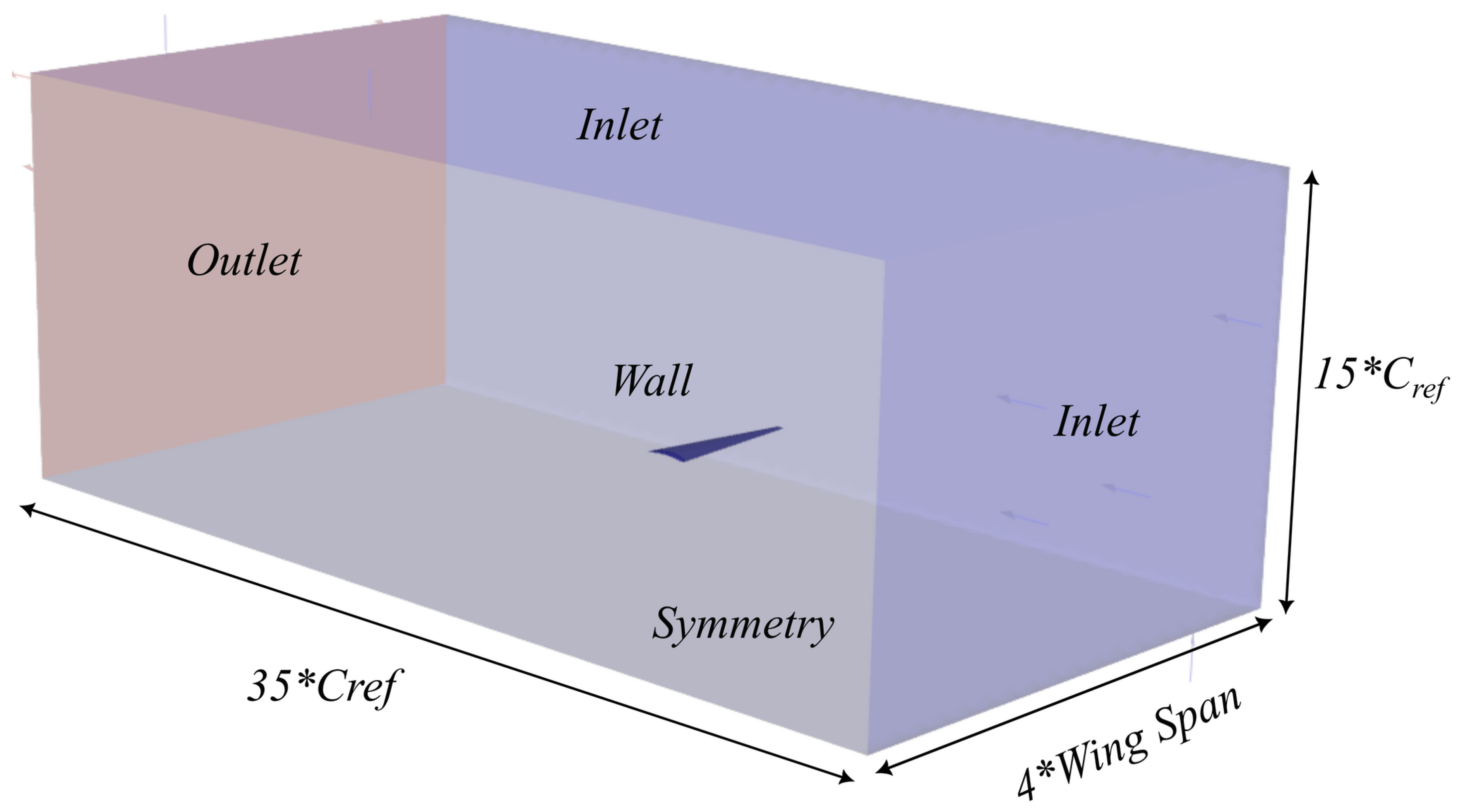
Figure 2.
CFD mesh around the wing.
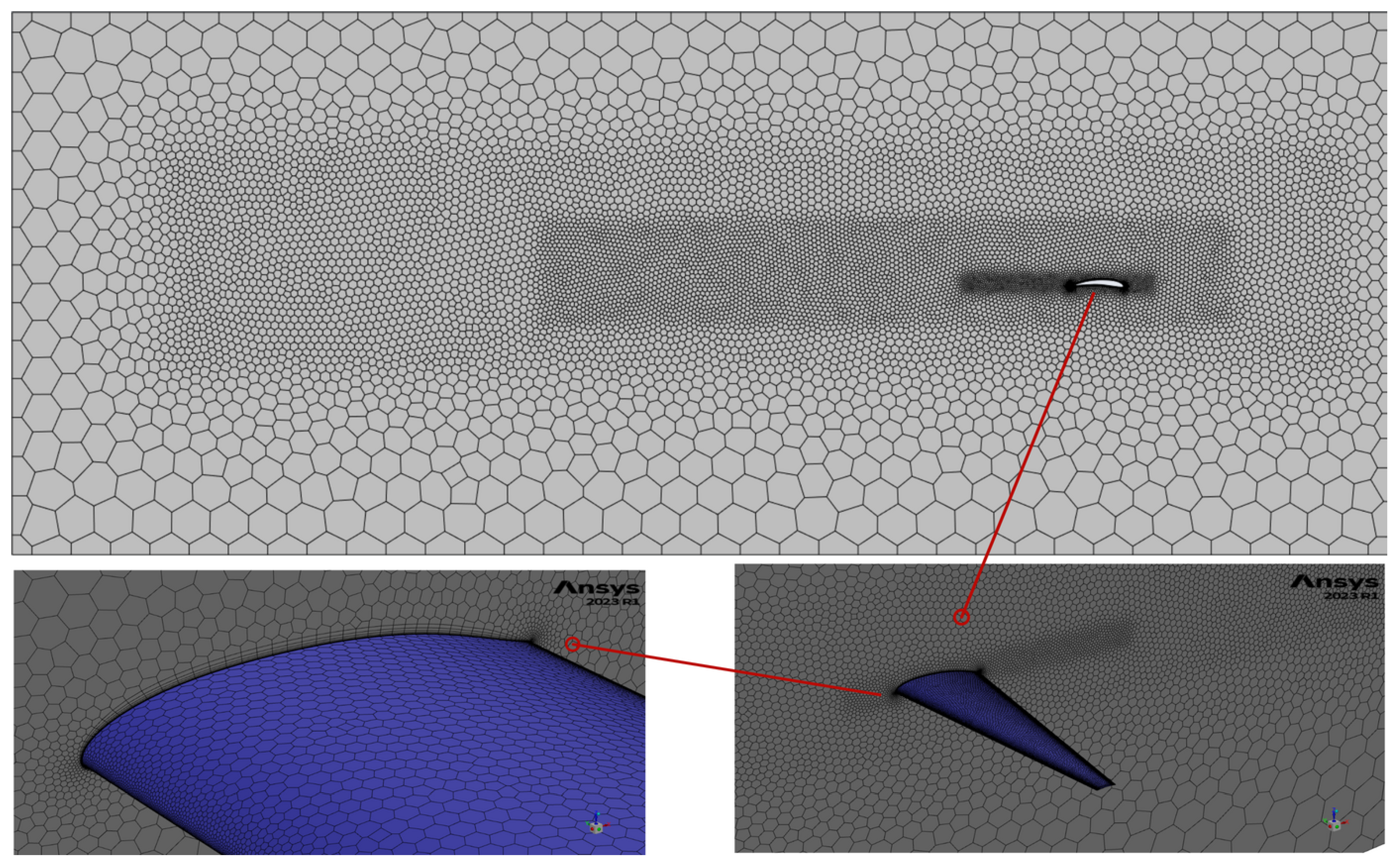
Figure 3.
and vs number of domain cells − Mesh independence study.
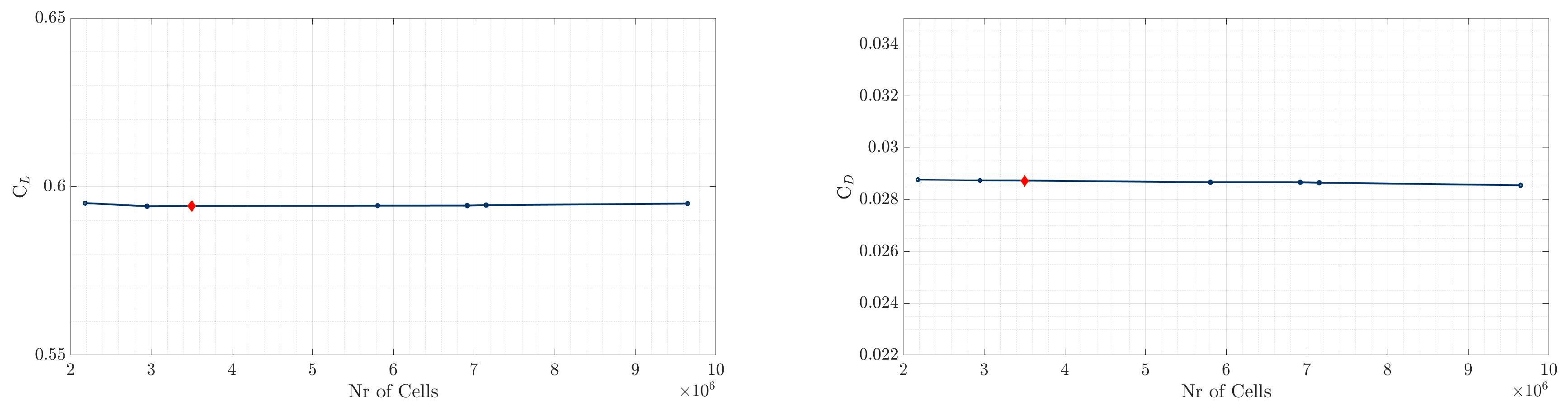
Figure 4.
1st SBO framework.
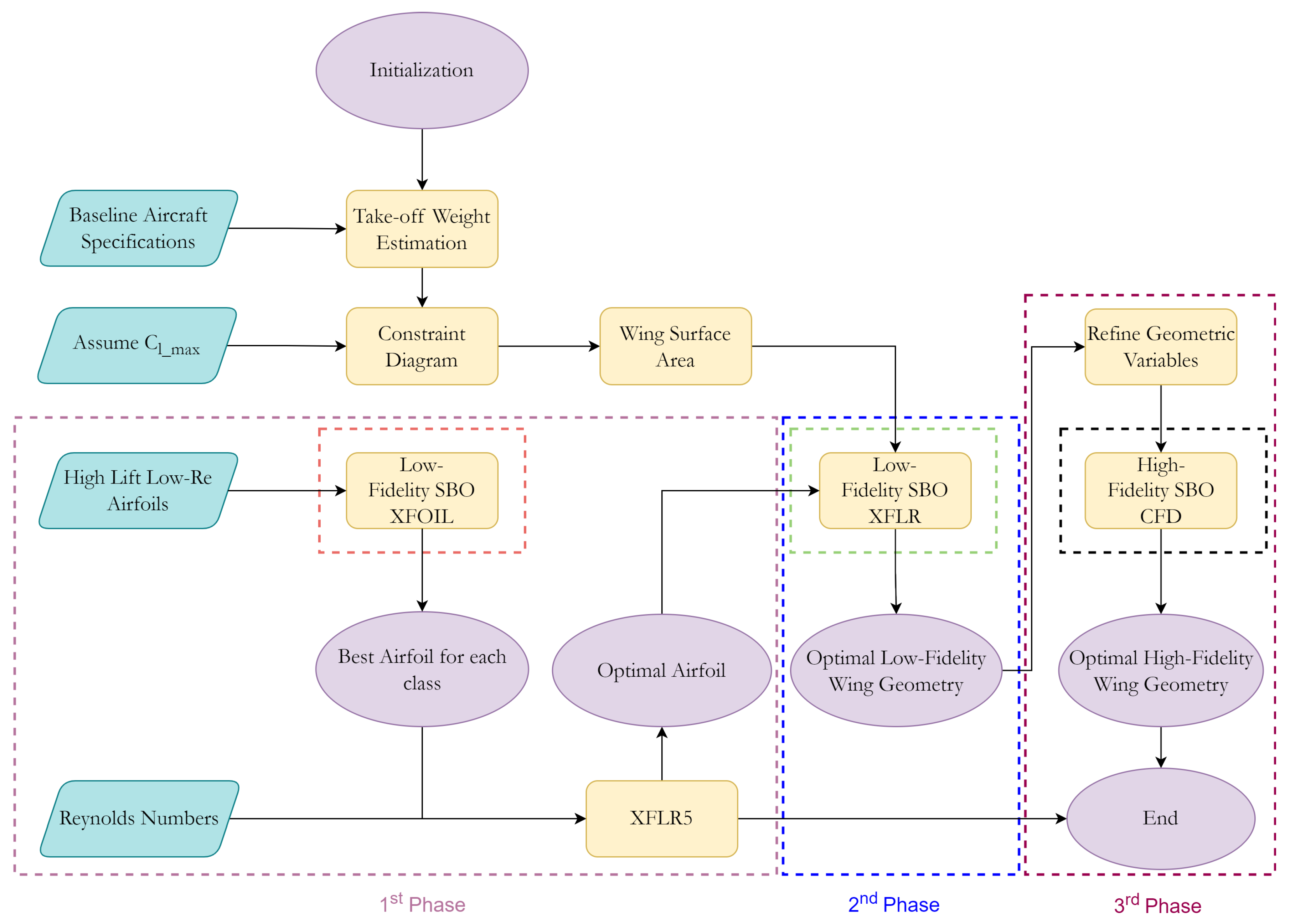
Figure 5.
2nd SBO framework.
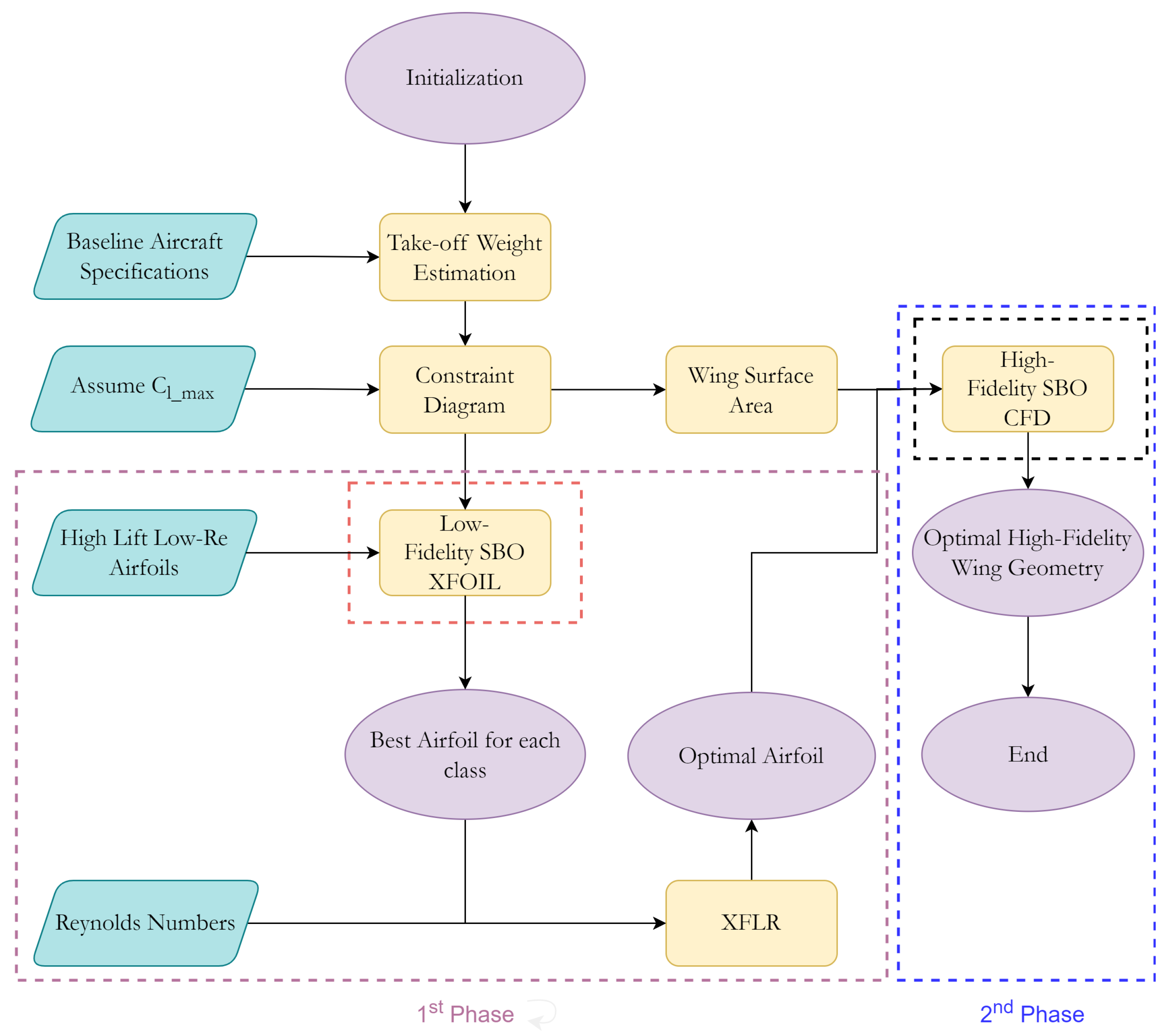
Figure 6.
General SBO framework.
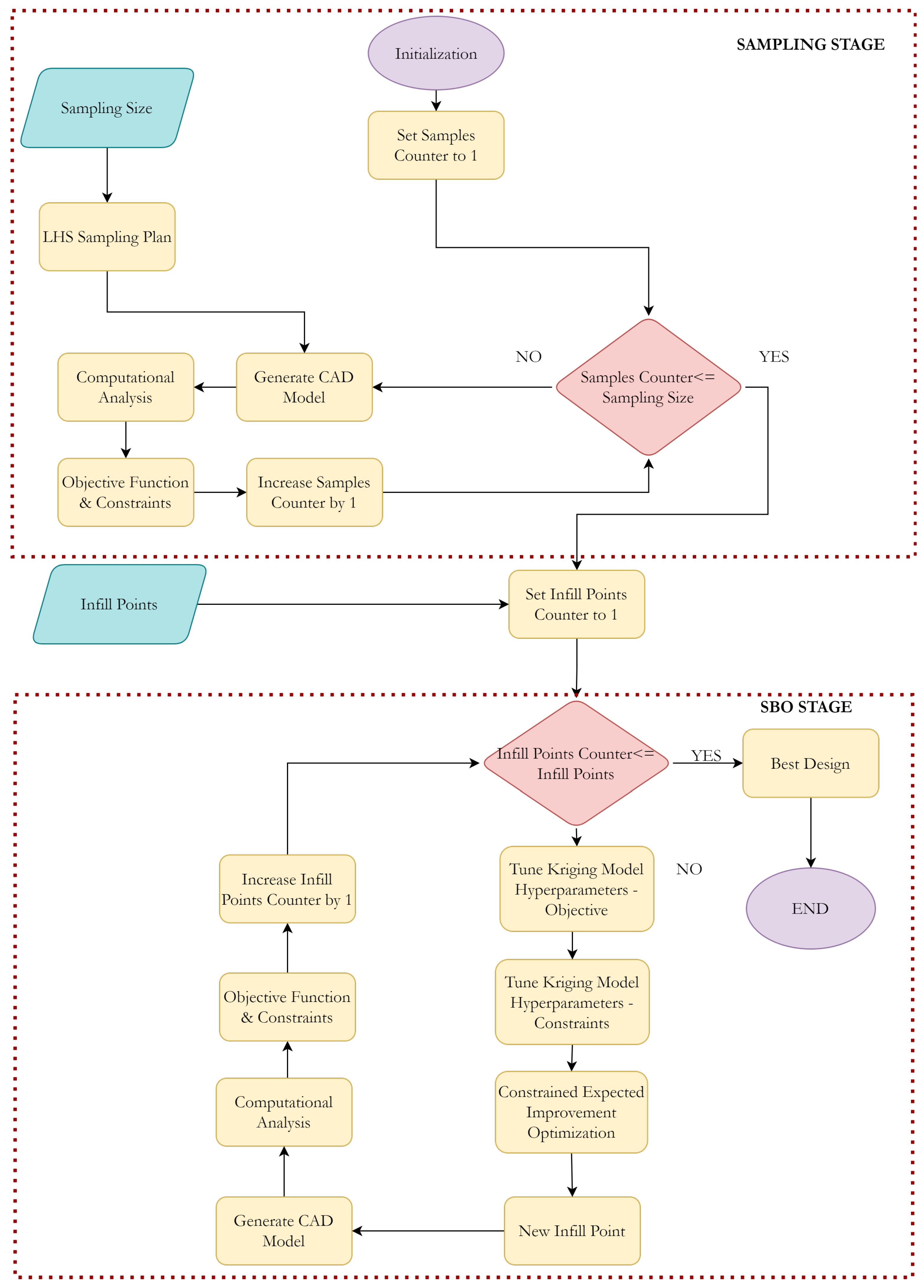
Figure 7.
CST airfoil parameterization for DAE-31 (a), Eppler-423 (b), NACA-6412 (c) and NACA-7313 (d) airfoils.
Figure 7.
CST airfoil parameterization for DAE-31 (a), Eppler-423 (b), NACA-6412 (c) and NACA-7313 (d) airfoils.
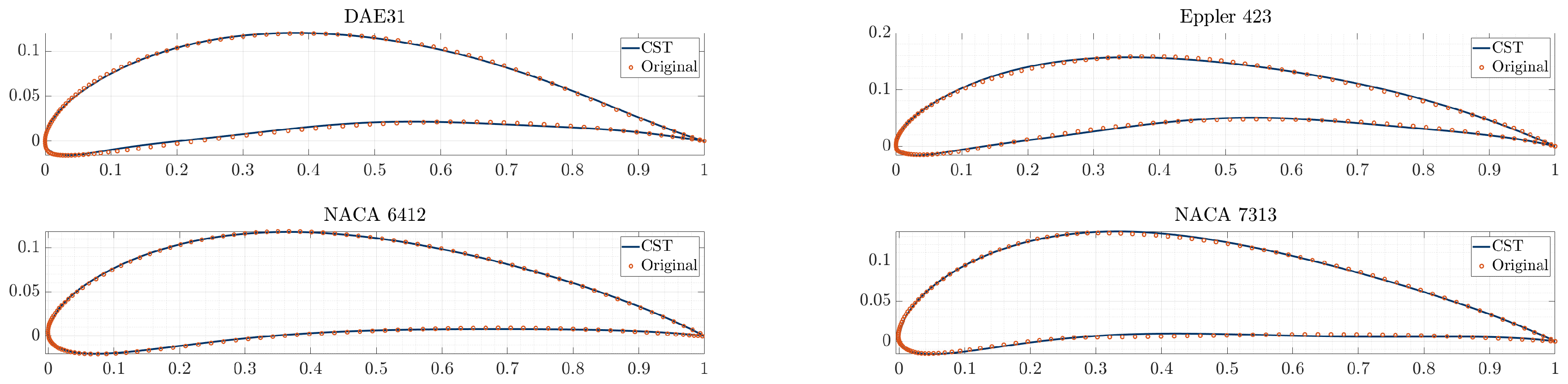
Figure 12.
Optimal wing configuration of 2nd phase of the 1st SBO.
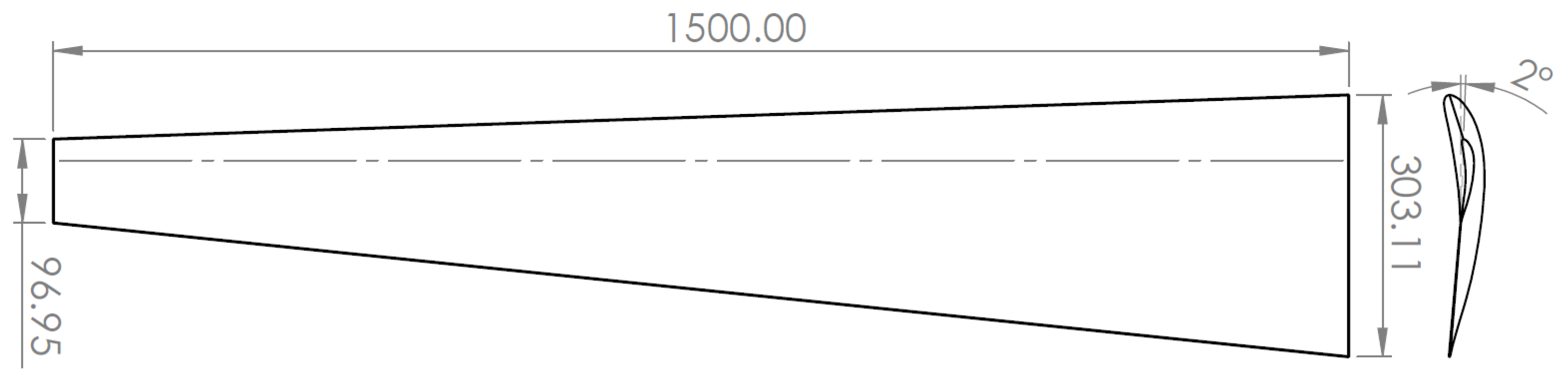
Figure 13.
Optimal wing configuration of 2nd phase of the 1st SBO airfoil.
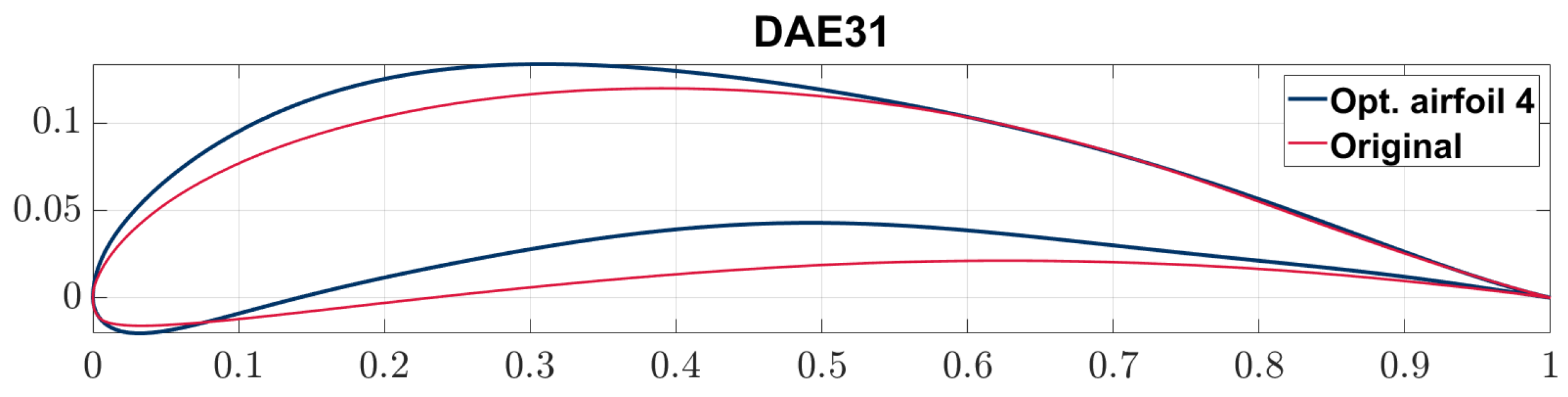
Figure 20.
Optimal wing geometries aerodynamic results comparison - (a), (b), (c) and (d) versus .
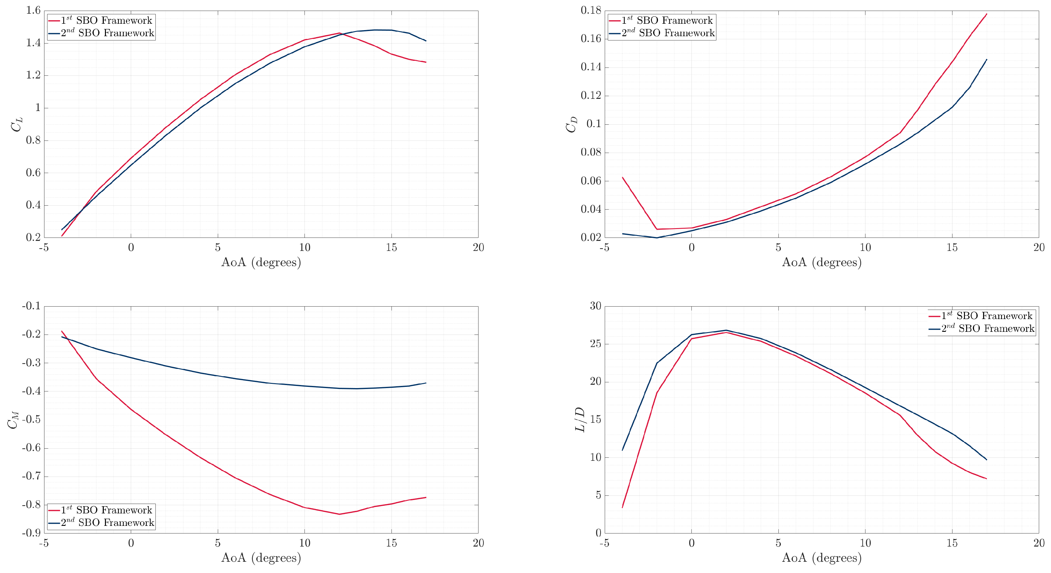
Figure 21.
Optimal wing configuration of both SBO frameworks.
Table 1.
UAV requirements and mission flight characteristics.
| Characteristic | Symbol |
|---|---|
| UAV type | Fixed-wing |
| Propulsion system | Battery-powered electric |
| Wingspan | m |
| UAV length | m |
| Maximum take-off weight | |
| Take-off | Catapult take-off |
| Cruise speed | |
| Loiter Speed | |
| Climb Speed | |
| Operational altitude |
Table 2.
CST parameterization variables for each airfoil.
| Variable | DAE 31 | Eppler 423 | NACA 6412 | NACA 7313 |
| 0.22000 | 0.30000 | 0.30000 | 0.24000 | |
| 0.36000 | 0.50000 | 0.43000 | 0.36000 | |
| 0.27122 | 0.33000 | 0.27000 | 0.27000 | |
| 0.42200 | 0.47000 | 0.38000 | 0.38000 | |
| 0.21481 | 0.50000 | - | - | |
| -0.14000 | -0.15000 | - | - | |
| 0.16000 | 0.20000 | - | - | |
| -0.22000 | -0.20000 | -0.11000 | -0.12000 | |
| 0.35000 | 0.47000 | 0.15500 | 0.08000 | |
| -0.11929 | 0.02000 | -0.08500 | -0.02000 | |
| 0.15378 | 0.16000 | 0.10000 | 0.08000 | |
| 0.10449 | 0.26091 | - | - |
Table 3.
Upper and lower boundaries of DAE31 CST variables.
| Variable | 1st lb | 1st ub | 2nd lb | 2nd ub | 3rd lb | 3rd ub | 4th lb | 4th ub |
| -20% | +20% | -30% | +30% | -30% | +30% | -35% | +35% | |
| -20% | +20% | -30% | +30% | -30% | +30% | -35% | +35% | |
| -20% | +20% | -25% | +25% | -30% | +30% | -30% | +30% | |
| -15% | +15% | -15% | +15% | -25% | +25% | -20% | +20% | |
| -5% | +5% | -5% | +5% | -10% | +10% | -5% | +5% | |
| -20% | +20% | -30% | +30% | -30% | +30% | -35% | +35% | |
| -20% | +20% | -30% | +30% | -30% | +30% | -35% | +35% | |
| -20% | +20% | -25% | +25% | -30% | +30% | -30% | +30% | |
| -15% | +15% | -20% | +20% | -30% | +30% | -25% | +25% | |
| -15% | +15% | -15% | +15% | -25% | +25% | -15% | +15% | |
| -10% | +10% | -10% | +10% | -25% | +25% | -10% | +10% | |
| -20% | +20% | -20% | +20% | -10% | +10% | -5% | +5% |
Table 4.
Upper and Lower Boundaries of Eppler-423, NACA-6412 and NACA-7313 CST variables.
| Variable | Eppler 423 lb | Eppler423 ub | NACA6412 lb | NACA6412 ub | NACA7313 lb | NACA7313 ub |
| -30% | +30% | -30% | +30% | -30% | +30% | |
| -30% | +30% | -25% | +25% | -25% | +25% | |
| -25% | +25% | -20% | +20% | -20% | +20% | |
| -20% | +20% | -10% | +10% | -10% | +10% | |
| -5% | +5% | - | - | - | - | |
| -30% | +30% | - | - | - | - | |
| -30% | +30% | - | - | - | - | |
| -25% | +25% | -30% | +30% | -30% | +30% | |
| -25% | +25% | -25% | +25% | -25% | +25% | |
| -20% | +20% | -20% | +20% | -20% | +20% | |
| -15% | +15% | -10% | +10% | -10% | +10% | |
| -5% | +5% | - | - | - | - |
Table 5.
Upper and lower boundaries of each geometric variable - 2nd phase of the 1st SBO framework.
Table 5.
Upper and lower boundaries of each geometric variable - 2nd phase of the 1st SBO framework.
| Geometric Variable | Lower Boundary | Upper Boundary |
| 6.5 | 15 | |
| 0.2 | 1 | |
| 0o | 30o | |
| 2o |
Table 6.
20 infill points geometric characteristics of favourable airfoil conf. - 2nd phase (SBO with XFLR5).
Table 6.
20 infill points geometric characteristics of favourable airfoil conf. - 2nd phase (SBO with XFLR5).
| Wing conf. | b | ||||||
| 41 | 15.00 | 0.20 | 0.00 | -4.00 | 3.00 | 0.33 | 0.07 |
| 42 | 15.00 | 0.20 | 4.34 | -0.25 | 3.00 | 0.33 | 0.07 |
| 43 | 14.07 | 0.20 | 28.07 | -4.00 | 2.91 | 0.34 | 0.07 |
| 44 | 10.75 | 0.20 | 0.00 | 2.00 | 2.54 | 0.39 | 0.08 |
| 45 | 15.00 | 1.00 | 0.00 | -4.00 | 3.00 | 0.20 | 0.20 |
| 46 | 15.00 | 1.00 | 30.00 | 2.00 | 3.00 | 0.20 | 0.20 |
| 47 | 15.00 | 0.55 | 12.20 | 2.00 | 3.00 | 0.26 | 0.14 |
| 48 | 15.00 | 0.39 | 0.00 | -4.00 | 3.00 | 0.29 | 0.11 |
| 49 | 15.00 | 0.20 | 11.25 | 2.00 | 3.00 | 0.33 | 0.07 |
| 50 | 6.50 | 1.00 | 0.00 | 2.00 | 1.97 | 0.30 | 0.30 |
| 51 | 15.00 | 0.60 | 30.00 | 2.00 | 3.00 | 0.25 | 0.15 |
| 52 | 15.00 | 0.98 | 26.48 | -4.00 | 3.00 | 0.20 | 0.20 |
| 53 | 15.00 | 0.32 | 0.01 | 2.00 | 3.00 | 0.303 | 0.097 |
| 54 | 15.00 | 0.45 | 17.47 | -4.00 | 3.00 | 0.28 | 0.12 |
| 55 | 15.00 | 0.25 | 7.50 | 1.24 | 3.00 | 0.32 | 0.08 |
| 56 | 14.94 | 0.85 | 0.12 | 1.99 | 2.99 | 0.22 | 0.18 |
| 57 | 15.00 | 0.50 | 27.87 | -3.46 | 3.00 | 0.27 | 0.13 |
| 58 | 15.00 | 0.20 | 30.00 | 2.00 | 3.00 | 0.33 | 0.07 |
| 59 | 6.50 | 1.00 | 30.00 | -4.00 | 1.97 | 0.30 | 0.30 |
| 60 | 10.75 | 0.20 | 0.00 | -4.00 | 2.54 | 0.39 | 0.08 |
Table 7.
Low-fidelity results of 20 infill points of favorable airfoil conf. - 2nd phase (SBO with XFLR5).
Table 7.
Low-fidelity results of 20 infill points of favorable airfoil conf. - 2nd phase (SBO with XFLR5).
| Wing conf. | |||||||
| 41 | 15.0 | 2.034 | 25.803 | 5.486 | 0.632 | 0.032 | 19.750 |
| 42 | 12.0 | 1.830 | 26.751 | 4.785 | 0.795 | 0.03 | 26.500 |
| 43 | 14.0 | 1.795 | 26.107 | 5.021 | 0.592 | 0.038 | 15.579 |
| 44 | 14.0 | 1.908 | 23.199 | 5.114 | 0.689 | 0.032 | 21.531 |
| 45 | 14.5 | 1.836 | 24.913 | 4.583 | 0.509 | 0.044 | 11.568 |
| 46 | 17.0 | 2.036 | 22.713 | 4.742 | 0.679 | 0.04 | 16.975 |
| 47 | 13.5 | 1.991 | 25.679 | 5.372 | 0.752 | 0.033 | 22.788 |
| 48 | 16.0 | 2.077 | 26.260 | 5.486 | 0.588 | 0.039 | 15.077 |
| 49 | 10.0 | 1.673 | 27.341 | 5.429 | 0.731 | 0.029 | 25.207 |
| 50 | 17.0 | 1.860 | 20.021 | 4.312 | 0.639 | 0.032 | 19.969 |
| 51 | 16.0 | 2.006 | 24.611 | 4.885 | 0.683 | 0.038 | 17.974 |
| 52 | 20.0 | 2.061 | 24.433 | 4.799 | 0.459 | 0.048 | 9.563 |
| 53 | 13.5 | 2.013 | 26.748 | 5.472 | 0.748 | 0.03 | 24.933 |
| 54 | 16.5 | 2.065 | 26.680 | 5.336 | 0.574 | 0.041 | 14.000 |
| 55 | 12.5 | 1.901 | 27.209 | 5.472 | 0.726 | 0.029 | 25.034 |
| 56 | 13.5 | 2.001 | 24.778 | 5.343 | 0.768 | 0.034 | 22.588 |
| 57 | 18.0 | 2.073 | 26.162 | 5.021 | 0.550 | 0.043 | 12.791 |
| 58 | 9.5 | 1.494 | 27.419 | 4.985 | 0.671 | 0.035 | 19.171 |
| 59 | 20.0 | 1.719 | 19.068 | 4.018 | 0.396 | 0.053 | 7.472 |
| 60 | 16.0 | 1.982 | 22.289 | 5.136 | 0.594 | 0.036 | 16.500 |
Table 8.
Upper and lower boundaries of each geometric variable - 3rd phase of the 1st SBO framework.
Table 8.
Upper and lower boundaries of each geometric variable - 3rd phase of the 1st SBO framework.
| Geometric Variable | Lower Boundary | Upper Boundary |
| 0.2 | 0.55 | |
| 0o | 10o | |
| 2o |
Table 11.
20 infill points geometric characteristics - 2nd phase (SBO with CFD).
| Wing conf. | b | ||||||
| 41 | 15.00 | 0.20 | 3.20 | -1.00 | 3.00 | 0.333 | 0.067 |
| 42 | 15.00 | 0.20 | 3.75 | 2.00 | 3.00 | 0.333 | 0.067 |
| 43 | 9.62 | 0.20 | 0.23 | 2.00 | 2.40 | 0.416 | 0.083 |
| 44 | 15.00 | 0.58 | 1.87 | 2.00 | 3.00 | 0.253 | 0.147 |
| 45 | 15.00 | 1.00 | 0.00 | 2.00 | 3.00 | 0.200 | 0.200 |
| 46 | 15.00 | 0.36 | 3.24 | 0.50 | 3.00 | 0.294 | 0.106 |
| 47 | 13.67 | 0.40 | 0.00 | 2.00 | 2.86 | 0.299 | 0.120 |
| 48 | 15.00 | 0.20 | 7.10 | -4.00 | 3.00 | 0.333 | 0.067 |
| 49 | 15.00 | 0.96 | 0.00 | -4.00 | 3.00 | 0.204 | 0.196 |
| 50 | 15.00 | 0.60 | 0.00 | 0.69 | 3.00 | 0.250 | 0.150 |
| 51 | 15.00 | 0.35 | 0.00 | -4.00 | 3.00 | 0.296 | 0.104 |
| 52 | 12.74 | 0.65 | 3.62 | 2.00 | 2.76 | 0.263 | 0.171 |
| 53 | 15.00 | 0.20 | 3.75 | -0.85 | 3.00 | 0.333 | 0.067 |
| 54 | 15.00 | 0.20 | 7.50 | -4.00 | 3.00 | 0.333 | 0.067 |
| 55 | 15.00 | 0.20 | 1.72 | 2.00 | 3.00 | 0.333 | 0.067 |
| 56 | 15.00 | 0.59 | 0.00 | 2.00 | 3.00 | 0.252 | 0.148 |
| 57 | 15.00 | 0.25 | 0.00 | 1.72 | 3.00 | 0.320 | 0.080 |
| 58 | 15.00 | 0.40 | 2.81 | 0.69 | 3.00 | 0.285 | 0.115 |
| 59 | 10.49 | 0.20 | 0.00 | 2.00 | 2.51 | 0.399 | 0.080 |
| 60 | 15.00 | 1.00 | 0.00 | -4.00 | 3.00 | 0.200 | 0.200 |
Table 12.
High-fidelity results of 20 infill points - 2nd phase (SBO with CFD).
| Wing conf. | |||||||
| 41 | 15 | 1.469 | 26.614 | 5.581 | 0.616 | 0.024 | 25.729 |
| 42 | 14 | 1.477 | 26.693 | 5.535 | 0.664 | 0.025 | 26.421 |
| 43 | 15 | 1.450 | 22.353 | 5.146 | 0.614 | 0.027 | 22.353 |
| 44 | 14 | 1.494 | 25.978 | 5.535 | 0.697 | 0.027 | 25.924 |
| 45 | 14 | 1.482 | 24.702 | 5.524 | 0.704 | 0.028 | 24.702 |
| 46 | 14 | 1.482 | 26.845 | 5.610 | 0.648 | 0.025 | 26.251 |
| 47 | 14 | 1.490 | 25.566 | 5.518 | 0.678 | 0.027 | 25.566 |
| 48 | 15 | 1.456 | 26.362 | 5.455 | 0.571 | 0.023 | 24.520 |
| 49 | 16 | 1.388 | 26.230 | 5.529 | 0.450 | 0.021 | 21.904 |
| 50 | 14 | 1.480 | 26.378 | 5.541 | 0.653 | 0.025 | 25.885 |
| 51 | 16 | 1.445 | 26.377 | 5.701 | 0.535 | 0.022 | 24.040 |
| 52 | 14 | 1.490 | 24.282 | 5.346 | 0.686 | 0.028 | 24.282 |
| 53 | 15 | 1.470 | 26.653 | 5.581 | 0.620 | 0.024 | 25.809 |
| 54 | 15 | 1.455 | 26.383 | 5.621 | 0.571 | 0.023 | 24.547 |
| 55 | 14 | 1.475 | 26.658 | 5.529 | 0.662 | 0.025 | 26.373 |
| 56 | 14 | 1.497 | 25.978 | 5.547 | 0.698 | 0.027 | 25.923 |
| 57 | 14 | 1.478 | 26.699 | 5.552 | 0.663 | 0.025 | 26.379 |
| 58 | 14 | 1.480 | 26.781 | 5.615 | 0.653 | 0.025 | 26.252 |
| 59 | 15 | 1.457 | 23.121 | 5.243 | 0.625 | 0.027 | 23.121 |
| 60 | 16 | 1.387 | 26.161 | 5.529 | 0.446 | 0.020 | 21.749 |
Disclaimer/Publisher’s Note: The statements, opinions and data contained in all publications are solely those of the individual author(s) and contributor(s) and not of MDPI and/or the editor(s). MDPI and/or the editor(s) disclaim responsibility for any injury to people or property resulting from any ideas, methods, instructions or products referred to in the content. |
© 2025 by the authors. Licensee MDPI, Basel, Switzerland. This article is an open access article distributed under the terms and conditions of the Creative Commons Attribution (CC BY) license (http://creativecommons.org/licenses/by/4.0/).
Copyright: This open access article is published under a Creative Commons CC BY 4.0 license, which permit the free download, distribution, and reuse, provided that the author and preprint are cited in any reuse.


