
Submitted:
29 June 2023
Posted:
12 July 2023
You are already at the latest version
Abstract
Agricultural soils serve as crucial storage sites for soil organic carbon (SOC). Their appropriate management is pivotal for mitigating climate change. To evaluate spatial and temporal changes in SOC within agricultural fields, continuous monitoring is imperative. In-field data sets of Vis-NIR soil spectra were collected on a long-term experimental site using an on-the-go spectrophotometer. Data processing for continuous SOC prediction involves a two-steps modelling approach. In Step 1, a Partial Least Square (PLSR) regression model is trained to establish a relationship between the SOC content and the spectral information also including spectral preprocesisng. In Step 2, the predicted SOC content obtained from the PLSR models is interpolated using ordinary kriging. Among the tested spectral preprocessing techniques and semivariogram models, SG and gapDer preprocessing along with a Gaussian semivariogram model, yielded the best performance resulting in a root mean square error of of 1.24 and 1.26 g kg-1. A striping effect due to the transect-based data collection was addressed by testing the effectiveness of extending the spatial separation distance, employing data aggregation, and defining the distribution based on treatment plots using block kriging. Overall, the results highlight the immense potential of on-the-go spectral Vis-NIR data for field-scale spatial-temporal monitoring of SOC.
Keywords:
soil organic carbon
; Vis-NIR spectroscopy
; monitoring
; pedometrics
1. Introduction
The spatial-temporal monitoring of soil organic carbon (SOC) in agricultural lands is instrumental in enabling climate-responsive agricultural management with a focus on enhancing SOC stocks. By analyzing SOC levels across different zones within a field and observing how they change over time, land managers and farmers can optimize their practices. This data-driven approach not only leads to improved soil health and productivity but also plays a significant role in climate change mitigation. One of the key global frameworks that recognize the importance of soil carbon sequestration is the Paris COP 21 Climate Change Agreement (UNFCCC, 2015), which emphasizes the critical role that soils play in capturing carbon dioxide from the atmosphere. By harnessing high-resolution spatial-temporal SOC data, it becomes possible to align agricultural practices with the goals outlined in this landmark agreement. In essence, monitoring SOC at a granular level empowers farmers to engage in precision carbon farming, adapt to climate variability, and contribute to global climate goals. The integration of advanced technologies like soil sensing technology is essential in collecting this data, and the collaboration among scientists, policymakers, and farmers can foster the development and adoption of practices that maximize SOC sequestration in line with the objectives of the Paris Agreement. Conventional chemical laboratory analysis has its limitations when it comes to data acquisition for soil properties, making it an unfeasible approach for extensive use (Stenberg et al., 2010). To address this, ancillary data is often incorporated alongside traditional soil sampling methods for constructing field maps. One particularly promising avenue in this regard is soil spectroscopy, which is a component of proximal sensing data. Proximal sensing involves using sensors that are either in direct contact with or close to the soil and soil spectroscopy is an emerging technique in this category. It is recognized as a cost-effective method that can amass high-density data at the field scale (Knadel et al., 2011). Soil spectroscopy entails the analysis of how soils interact with electromagnetic radiation, and it has been researched for its potential in predicting SOC among other properties (Corwin and Lesch, 2005). Although soil spectroscopy in the field is an area that is yet to be thoroughly explored, some studies demonstrate its potential through point measurements (Wetterlind et al., 2015; Cho et al., 2017; Viscarra Rossel et al., 2017). Moreover, there is a growing interest in the utilization of on-the-go sensors for soil spectroscopy, which has proven to be more appropriate for soil mapping applications (Huang et al., 2007; Muñoz and Kravchenko, 2011; Knadel et al., 2015). In conjunction with soil spectroscopy, remote sensing data can also be utilized. It is collected from sources such as satellites, airborne instruments, or unmanned aerial vehicles and can be used to estimate SOC through variables like NDVI, topographic indices, and multispectral imagery (Bartholomeus et al., 2011; Angelopoulou et al., 2019). However, it’s pertinent to consider that remote sensing has its own set of limitations, including spectral resolution, image quality, and data acquisition frequency.
Soil spectroscopy has emerged as a potent tool for monitoring SOC due to its ability to detect and analyze the interactions between electromagnetic radiation and soil constituents. In the VisNIR range (350-2500 nm), soil spectra exhibit weak overtones and combinations of fundamental vibrations caused by the bending and stretching of various soil compounds. This range is especially sensitive to organic matter, making it viable for SOC estimation (Ladoni et al., 2010). As of now, the state of the art in soil spectroscopy predominantly involves laboratory-based analyses. Under controlled conditions, soil samples are subjected to spectral measurements, and the data is analyzed to establish relationships between spectral characteristics and SOC content. Among the methods employed, partial least squares regression (PLSR) has been widely used as the standard analytical technique. PLSR efficiently handles the complex soil spectra by extracting the information that is most relevant to SOC, thus enabling the development of robust prediction models (Padarian et al., 2020). Attempts have been made to extend soil spectroscopy to field conditions for continuous, field-scale SOC monitoring. This involves various approaches such as UAV-based, airborne remote sensing, and proximal on-the-go sensing. For instance, Unmanned Aerial Vehicles (UAVs) can carry sensors that capture soil spectra over large areas. Similarly, airborne remote sensing platforms can provide spectral data at broader scales. However, these methods can be limited by spectral resolution, image quality, and frequency of acquisitions (Bartholomeus et al., 2011; Angelopoulou et al., 2019). Proximal on-the-go sensing represents a more direct approach, where sensors are close to the soil and can capture high-density data. However, implementing soil spectroscopy in the field is inherently challenging due to various environmental factors affecting the spectra. The resulting uncertainties in the SOC-VisNIR relationship models can pose limitations for field mapping and the transferability of the models to other sites (Ge et al., 2011). Long-term field experiments (LTEs) are strategically designed to evaluate the long-term effects of various agricultural management practices on soil properties and crop traits (Körschens, 2006). Their structured setup, which includes distinct treatment plots, is particularly conducive to monitoring SOC. By observing the influence of different practices on soil within the same experimental framework, LTEs provide rich, longitudinal data that is crucial for understanding how SOC levels change over time under various conditions. This makes LTEs an invaluable resource for making informed decisions about sustainable agricultural management with an emphasis on the vital role of SOC in soil health. This study aims to delve into the feasibility and potential of employing on-the-go VisNIR spectroscopy as a tool for spatial-temporal monitoring of SOC. A comprehensive modeling procedure is formulated and presented as a central component of this investigation. Additionally, the study meticulously examines the specific influence that each stage of the modeling procedure has on predictive uncertainty. Through this multifaceted approach, the study seeks to shed light on the capabilities and limitations of on-the-go VisNIR spectroscopy in accurately capturing the spatial and temporal variations in SOC.
2. Materials and Methods
2.1. Study area
Data was collected on the LTE site Static Fertilization Experiment in Bad Lauchstädt, Saxony-Anhalt, Germany (51°24' N, 11°53'E, 113 m a.s.l). The site is characterized by an average total annual precipitation of 470-540 mm and an average annual temperature of 8.5-9.0°C. The soil was described as Haplic Chernozem developed from loess (Altermann et al., 2005). Accordingly, it has a topsoil texture varying between highly clayey silt (Ut4) and highly silty clay (Tu4) according to the German soil survey system (Ad-hoc-AG Boden, 2005). The field experiment was initialized in 1902 by Schneidewind and Gröbler on an area of c. 4 ha (Merbach and Schulz, 2013) with eight subfields (Figure 1A) From the initital crop rotation of winter wheat, sugar beet, summer barley, and potato, the root crops were replaced by silage maize from 2015 onwards. Different crops in nearby fields started the agricultural rotation, ensuring that all crops are always produced concurrently on the experimental site. 30 dt of lime is applied to subfield one every four years in the spring. On subfield 8, legumes have been a part of the agricultural rotation every seventh and eighth year since 1926. The 288 plots as a whole vary according to how they were fertilized with minerals and organic fertilizer. One-third of each field is covered with farmyard manure applied at rates of 20 and 30 t ha-1, respectively, while the other third is left devoid of organic fertilizer. Mineral fertilizer is applied in various N, P, and K combinations. In 1978, the experimental site's subfields four and five were modified to examine additional fertilizer treatments involving varied levels of N in combination with an adapted organic fertilizer treatment. Körschens and Pfefferkorn (1998) go into greater detail.
2.2. Data collection
In September 2018, soil samples were collected from 100 different locations at depths ranging from 0 to 10 cm (Figure 1B). The samples were selected to cover the experimental site’s soil variability according to archive data. Two sampling designs were applied for this reason (Ellinger et al., 2019): 50 sampling points were selected according to stratified random sampling, the other 50 sampling points were selected by employing the Kennard–Stone algorithm (Kennard and Stone, 1969). Plot margins of 1.5 m were excluded from sampling. Before measuring carbon with dry combustion, the soil samples were air-dried, sieved (2 mm), and powdered. Total carbon was assessed using the elemental analyzer, vario EL cube CN (Elementar Analysensysteme GmbH), with three replicates conducted for each sample. While carbonates were initially measured, their values were found to be inconsequential and therefore were omitted from the analysis. As such, the total carbon measured was regarded as an indicator of SOC in this study. The observed SOC content is 19.6 g kg-1 with a range of 14-25 g kg-1, indicating a wide range of SOC values generated from different fertilization treatments.
Spectral measurements were made using a Veris® Vis-NIR spectrophotometer manufactured by Veris Technologies, Inc (hence referred to as Veris). The Veris is equipped with an Ocean Optics USB4000 instrument (300 to 1100 nm) and a Hamamatsu TG series mini-spectrometer (1100 to 2200 nm), with a resolution of 4-6 nm. Due to logistical constraints, Veris field measurements were completed a year following soil collection in September 2019. The data were acquired at different dates to cover the entire field, the soil water content at the moment of measurement was in the range of 15-30%. Several transects with a distance of 3-4 m were recorded covering the entire field and considering passing through the soil sampling points, obtaining about 10,000 data points (Figure 1). The spatial location of the on-the-go spectral measurements was initially recorded using the Veris instrument. These original GPS coordinates were then corrected and refined using a high-precision GNSS instrument, ensuring enhanced spatial accuracy and reliability in the positioning of the spectral measurements. Meanwhile, the spatial location of the soil sampling points was recorded directly using the GNSS instrument. The Veris spectrometer is built in a shank that is pulled through the soil by a tractor with a measurement depth of about 12 cm; measurements are taken through a sapphire window located on the shank's bottom. Approximately 20 spectra are captured each second (Christy, 2008). The 400-2200 nm spectral range was used for the model creation.
2.3. Data preprocessing
The PCOut function in the R-package mvoutlier was used to evaluate the soil spectra for outliers per LTE plot (Filzmoser and Gschwandtner, 2018). The scattering effects on the spectral signal were then reduced using various preprocessing approaches. The four combinations used were: Savitzky-Golay (SG; Savitzky and Golay, 1964), Savitzky-Golay + continuum removal (SGCR; Clark and Roush, 1998), gap segment method (gapDer; Hopkins, 2003), and multiplicative scatter correction (MSC, Martens et al., 1983). Details are given in Table 1. The prospectr R-package was used to obtain the SG, SGCR, and gapDer, and the pls R-package was used to obtain the MSC (Mevik et al., 2019).
2.4. Model training and evaluation
Model training was conducted in a two-step approach according to Figure 2. In Step 1 a regression model (R-model) is trained to relate the SOC content to the spectral information. In Step 2 the thereby obtained predictions of the SOC content are interpolated by ordinary kriging (K-model) to generate spatially continuous predictions throughout the area. We will refer to it as R+K modeling approach. It is not to be confused with regression kriging which would first build a regression model and then interpolate the residuals. Regression kriging would only be feasible if we would have continuous spectral measurements throughout the area. However, this is not the case when on-the-go proximal sensing data is collected by sensors with a small spatial footprint. First of all the 10 spectral measurements of the surrounding of each sampling point were averaged and assigned to the respective sampling point. Together with the average SOC value per sampling point, these data form the XYdata A. In Step 1 of the modeling procedure, these data A are then used to train PLSR models by a nested k-fold cross-validation (CV) procedure. Each training set of the outer CV loop was again subdivided into k folds in the inner CV loop to allow for model tuning, i.e. to determine the number of components. The PLSR model was then trained with and evaluated with . After applying the respective PLSR model to all those spectra which were not assigned to any sampling point, the resulting SOC predictions were combined with to form Ydata B, the input data for Step 2 of the modeling procedure. In Step 2 of the modeling procedure, the Ydata B were spatially stratified into k folds making sure that each fold contained spectral measurement points from all LTE plots. This inner CV loop of modeling Step 2 was then used to determine the semivariogram parameters for ordinary kriging (OK). The K-models were again evaluated by the same test sets as the R-models. Data subdivision for the nested CV accounted for possible spatial autocorrelation between training and test data in two aspects: (1) nearby sampling points were assigned to the same fold, and (2) spectral measurements in the near surrounding of those spectral measurements assigned to the sampling points to generate the XYdata were excluded when building the K-model. The overall CV procedure was conducted with and repeated 5 times, resulting in 25 R + K models and 25 spatially continuous predictions for each of the four differently preprocessed datasets and the three different semivariogram models: Spherical, Exponential, and Gaussian. Equal data subdivisions were used to allow for direct comparison. The root mean square error (RMSE) was used to evaluate model performance. Spatially continuous predictions were realized with 1 m spatial resolution. Due to the structure of the LTE (divided into plots with different treatments), the maximum spatial separation distance considered to construct the experimental variogram was 10 m. Alternative kriging approaches including pair of point aggregation and block kriging were also applied to pay tribute to data collection on an LTE. The PLSR models were trained with R-package pls, and the geospatial analysis was done using the R-package gstat (Pebesma, 2004). The plots were created using the R-packages ggplot2 (Wickman, 2016) and lattice (Saknar, 2008).
3. Results and discussion
3.1. Model structure
Figure 3 shows distinct patterns in the optimal number of PLSR component for each preprocessing method. The SG and SGCR methods generally required a higher number of components, indicating a need to capture finer details and variations in the data. This aligns with the smoothing and denoising properties of the SG filter and the inclusion of continuum removal in the SGCR method to preserve intricate features. In contrast, the gapDer and MSC methods tended to require fewer components, suggesting a concise representation of the data. The gapDer method effectively reduced noise and identified important spectral regions through gap segmentation, while the MSC method corrected for multiplicative effects, enhancing the accuracy of the spectral information.
Figure 4 shows the K-models corresponding to the R-model-predicted SOC of the on-the-go spectral data (Ydata B). When comparing the K-models built from the predictions on behalf of the differently preprocessed data, there is a similarity in the spatial structure, although the semivariance in SG and gapDer is slightly lower. However, there is a difference in the parameter values between semivariogram models. The Spherical model exhibited a smoother and more gradual change in the variable being measured, indicating a lower level of small-scale variability. This implies that neighboring data points within a certain distance tend to have similar values. In terms of maximum variability, the Spherical model displayed moderate to high levels, suggesting significant variations across the dataset. Furthermore, the Spherical model had larger spatial correlation ranges, indicating a wider extent of influence between data points. The Exponential model displayed moderate levels of small-scale variability, characterized by a decay pattern where nearby data points were more similar than those farther apart. Its spatial correlation range was generally smaller than that of the Spherical model, indicating a more rapid decrease in correlation with increasing distance. The Gaussian model, however, exhibited similar patterns of small-scale and maximum variability to the Exponential model. It captured intermediate levels of small-scale variability, displaying a balance between the smoother Spherical model and the decay pattern of the Exponential model. The Gaussian model's spatial correlation range was smaller than both the Spherical and Exponential models, suggesting a more localized influence of neighboring points. This suggests that data points that are nearby have a stronger impact on each other, while the impact diminishes rapidly as the distance increases.
3.2. Performance metrics of PLSR and OK
Figure 5 is presenting the predictive model performance of the PLSR models. The best models were the ones using SG and gapDer with a median RMSER value below 1.6 g kg-1. They also indicate a lower dispersion compared to the other two models as is observable in the comparison of predicted versus measured values (Figure 6). SG is a common method that mainly smoothes the original signal to remove multiplicative and additive effects (Dotto et al., 2018), meanwhile, the gapDer method works by derivate specific segments of the signal (Rinnan et al., 2009). The gapDer is the preprocessing method with a lower number of wavelengths used compared with the others selected in this study, thus the reduction of the model complexity (Tabatabai et al., 2019) could have a positive effect in this case. The differences observed between preprocessing methods remark the importance of selecting an adequate method, because there is no standard procedure even under laboratory conditions due to the type and amount of preprocessing required is data specific for soil (Viscarra Rossel et al., 2006, Stenberg and Viscarra Rossel., 2010). The overall predictive model performance of modeling Step 1 + Step 2 (R+K model) is presented in Figure 7 and the scatter plot with a line of equality is in Figure 8. By including modeling Step 2, the overall predictive performance was further improved. The best predictive performance for Step 2 was achieved with the Gaussian model. Accordingly, the best results were obtained with the combination SG-Gaussian (= 1.24 g kg-1, = 0.84) and gapDer-Gaussian (==1.26 g k-1, = 0.82). The observable pattern of the dispersion in the predictions (Figure 8) has more similarities concerning the preprocessing method rather than with regard to the semivariogram model.
Another aspect to consider is the spatial distribution of the residuals. Figure 9 presents an example for the SG-Gaussian and gapDer-Gaussian methods. Both approaches present similarities in the distribution of the residuals, and the majority is in the range of -0.5 – 0.5 g kg-1. There is no clear trend based on the plot size or the cluster division used for the sampling design, although areas with higher SOC showed higher interquartile range values and vice versa in the case of areas with low SOC values.
3.3. Spatially continuous predictions of SOC
The spatially continuous prediction of SOC presented similar patterns independent of the combination of methods used for interpolation. As an illustration, Figure 10 presents the maps of the estimated SOC using the models with the best performance (SG-Gaussian and gapDer-Gaussian) and the difference in prediction between them. The SOC values presented a range of about 10-30 g kg-1, which is a wider range compared with the laboratory samples (14-25 g kg-1). Not only the pattern is similar between methods but also the differences in the prediction were low with the exception of some specific areas. Figure 11 displays the spatial predictions of the same models comparing the interquartile range distribution of 25 predictions for each one. In general, the median interquartile range is below 1 g kg-1 in both cases with small differences between them. Although the spatial variation is most homogeneous in the case of the SG-Gaussian model.
Predictive uncertainty descreased with the combined use of the R and K models. This improvement can be attributed to the similarity in spectral data among neighboring points located within the same treatment plot, indicating lower soil variation within the plot. Among the semivariogram models, the Gaussian model exhibited effective balancing of small-scale variability and spatial correlation. It displayed a rapid decrease in correlation with distance, emphasizing localized influences, and showcased a lower level of small-scale variability. These characteristics contributed to more accurate predictions compared to the Spherical and Exponential semivariogram models (Figure 4). It is worth noting that the maximum spatial separation distance used for the semivariogram model in this study was short (10 m), focusing on capturing influences within the plot. However, the effectiveness of the model may vary in different locations due to differences in plot size within the LTE. Therefore, selecting a model that accurately represents the spatial structure is crucial for reliable interpolation (Kravchenko, 2003). Notably, when examining the residuals, similar trends were observed across different combinations, with higher values tending to be underestimated and lower values tending to be overestimated. This behavior aligns with the smoothing effect of ordinary kriging, as it tends to smooth out the spatial process.
Previous studies used in situ soil spectral measurements (e.g. Sudduth et al., 1993, Mouazen et al., 2005), and some of them have used a Veris spectrometer (Christy, 2008; Muñoz and Kravchenko, 2011; Knadel et al., 2011; Knadel et al., 2015; Tabatabai et al., 2019). The model performance in our study presented better RMSE values to predict SOC compared with these studies (best RMSE=2.7 g kg-1), although our R2 was lower compared with Tabatabai et al. (2019) (R2= 0.90). While the comparison is not straightforward due to differences in the SOC range, field conditions, and model evaluation procedure, and no other study has used an on-the-go spectrometer in an LTE, our results presented high accuracy showing the potential of applying our approach to predict SOC at the field scale for monitoring.
Regarding the soil maps, different combinations resulted in similar SOC spatial distribution, which could be expected due to the high sampling density of the Veris measurements reducing the uncertainty of the spatial interpolation. A stripping effect in the SOC distribution maps was evident, it was caused due to the Veris transects measurements in one direction (Knadel et al., 2015) and due to the short maximum spatial separation distance considered for the experimental semivariograms. This effect could be changed with data aggregation using different approaches. To illustrate alternatives for mapping the field, Figure 12 is presenting maps using a Saviztky Golay-Gaussian model with pair of point aggregation (Figure 12A), another with extending the maximum spatial separation distance of the experimental semivariogram to 25 m (Figure 12B) and using block-kriging with blocks defined by the plot treatments (Figure 12C). By aggregating a pair of points the stripping effect is diminished but still visible. When extending the maximum spatial separation distance, the stripping effect disappears, and a more general SOC distribution is observed. Nevertheless, a generalization of the SOC distribution could mask the values of small plots and the spatial variation inside of the plots, so it could be better to be applied in fields with homogeneous management. In the case of using block-kriging, a map with blocks divided by the plot treatments is presented. Block kriging has been less used in soil mapping compared with point kriging methods (Cressie, 2006). Generally, it uses blocks of the same size to upscale point observations (Kang et al., 2017). In the LTE, the block-kriging approach could be an alternative to monitor SOC changes by having a unique value per plot treatment, although it will not represent the internal variation inside the plot.
Mapping SOC has also been studied with remote sensing using airborne and satellite platforms to cover extended areas although with lower precision. Consequently, it should be integrated with field and laboratory measurements and complementary ancillary data for better results (Croft et al., 2012). Our results showed the feasibility of using on-the-go soil spectra for mapping SOC with appropriate reliability, having an accuracy closer to laboratory measurements than remote sensing data. Nevertheless, different challenges appear when using field measurements due to environmental factors (Minasmy et al., 2011). For example, peaks in the spectral signal associated with soil water content can obscure peaks related to organic functional groups (Knadel et al., 2015). Our measurements were done on different days which also affected the variability of soil moisture, although with moisture that allowed to have good contact of the sensor with the soil and was not so wet to deeply mask local peaks associated with SOC. Another consideration is that the models tend to be site-specific so their transferability to other fields is difficult without collecting soil samples in new fields (Tabatabai et al. 2019).
4. Conclusions
The prediction of SOC using on-the-go field spectra demonstrated promising results. PLSR models, constructed with spectra close to the sampling location, effectively predicted the remaining Veris measurements, enabling the creation of high-resolution field maps. An enhancement in model performance was evident when PLSR was synergized with Ordinary Kriging (R+K model) to generate continuous predictions, making this combination particularly noteworthy.
The preprocessing methods Savitzky-Golay (SG) and gap derivative (gapDer) stood out for their efficacy, and this was further accentuated when paired with a Gaussian semivariogram model. The boost in model performance upon utilizing these methods suggests that there is inherent similarity in spectral data among neighboring areas and within identical treatment plots. This improvement emphasizes the potential significance of these techniques in efficiently capturing spatial patterns and dependencies in the context of SOC prediction.
When the different R+K model predictions were compared, a pronounced similarity in the spatial distribution of SOC was observed, which is consistent with the expectations due to the high-density data collected using Veris. Nonetheless, the striping effect became apparent due to the data being gathered in transects and the use of a relatively small maximum spatial separation distance for the semivariograms. Alleviating this striping effect could be achieved by extending the spatial separation distance, employing data aggregation techniques, or defining the distribution based on treatment plots (i.e. block kriging or similar methods). The applicability of data aggregation is contingent on the layout of the field and the specificity of the information sought. It is crucial to acknowledge that employing field soil spectroscopy for predicting SOC at field scale is an area still in development. However, the results of this study underscore the potential of this technique in the continuous monitoring of SOC. There is an imperative need for ongoing efforts to refine and establish standard practices for field soil spectroscopy measurements.
Funding
The project was supported by funds of the Federal Ministry of Food and Agriculture (BMEL) based on a decision of the Parliament of the Federal Republic of Germany via the Federal Office for Agriculture and Food (BLE) under the innovation support programme.
References
- Angelopoulou T, Tziolas N, Balafoutis A, Zalidis G, Bochtis D. Remote Sensing Techniques for Soil Organic Carbon Estimation: A Review. Remote Sensing. 2019; 11(6):676. [CrossRef]
- Altermann, M. , Rinklebe, J., Merbach, I., Körschens, M., Langer, U., and Hofmann, B.: Chernozem – Soil of the Year 2005, J. Plant Nutr. Soil Sc., 168, 725–740. [CrossRef]
- Bartholomeus, H., L. Kooistra, A. Stevens, M. Leeuwen, B. Wesemael, E. Ben-Dor, B. Tychon. 2011. Soil organic carbon mapping of partially vegetated agricultural fields with imaging spectroscopy. International Journal of Applied Earth Observation and Geoinformation 13 (1): 81-88.
- Cho, Y. , Sudduth, K. Drummond, S.T. 2017. Profile soil property estimation using a Vis-Nir-Ec-Force probe. Transactions of the ASABE. 60. 683-692. 10.13031/trans.12049.
- Christy, C.D. 2008. Real-time measurement of soil attributes using on-the-go near infrared reflectance spectroscopy, Computers and Electronics in Agriculture, 61 (1): 10-19. [CrossRef]
- Clark, R. , & Roush, T. 1984. Reflectance Spectroscopy: Quantitative Analysis Techniques for Remote Sensing Applications. Journal of Geophysical Research 89(B7), 6329-6340 198410.1029/JB089iB07p06329.
- Croft, H., N. J. Kuhn, K. Anderson. ‘‘On the Use of Remote Sensing Techniques for Monitoring Spatio-Temporal Soil Organic Carbon Dynamics in Agricultural Systems’’. Catena. 2012. 94: 64-75.
- Cressie, N. 2006. Block Kriging for Lognormal Spatial Processes. Mathematical Geology. 38. 413-443. 10.1007/s11004-005-9022-8.
- Dotto, A. Dalmolin, R. Caten, A., & Grunwald, S. 2018. A systematic study on the application of scatter-corrective and spectral-derivative preprocessing for multivariate prediction of soil organic carbon by Vis-NIR spectra. Geoderma. 314. 262-274. 10.1016/j.geoderma.2017.11.006.
- Ellinger, M. , Merbach, I., Werban, U., and Ließ, M. 2019. Error propagation in spectrometric functions of soil organic carbon, SOIL, 5, 275–288. [CrossRef]
- Friedman, J.H. Multivariate adaptive regressions splines. Ann. Stat.1991, 19, 1–67.
- Filzmoser, P. Gschwandtner, M. 2018. mvoutlier: Multivariate Outlier. Detection Based on Robust Methods. R package version 2.0.9. https://CRAN.R-project.org/package=mvoutlier.
- Ge, Y. , Morgan, C.Grunwald, S., Brown, D., Sarkhot, D. 2011. Comparison of soil reflectance spectra and calibration models obtained using multiple spectrometers. Geoderma. 161. 202-211. 10.1016/j.geoderma.2010.12.020.
- Guio Blanco, C. M. , Brito Gomez, V. M., Crespo, P., Ließ, M. 2018. Spatial prediction of soil water retention in a Páramo landscape: Methodological insight into machine learning using random forest. Geoderma, 316, 100–114. [CrossRef]
- Journel, A.G. , and Huijbregts, C.J. 1978. Mining geostatistics. Academic Press.
- Johnson, C.K., J. W. Doran, H.R. Duke, B.J. Wienhold, K.M. Eskridge, J.F. Shanahan. 2001. Field-scale conductivity mapping for delineating soil condition. Soil Sci. Soc. Am. J., 65:1829-1837. 1829. [Google Scholar]
- Hopkins, D.W. (2003). NIR news, 14(5), 10.Huang, X.W., S. Senthilkurnar, A. Kravchenko, K. Th elen, and J.G. Qi. 2007.Total carbon mapping in glacial till soils using near-infrared spectroscopy, Landsat imagery and topographical information. Geoderma 141:34–42. [CrossRef]
- Kang, Jian & Jin, Rui & Zhang, Yang. 2017. Block Kriging With Measurement Errors: A Case Study of the Spatial Prediction of Soil Moisture in the Middle Reaches of Heihe River Basin. IEEE Geoscience and Remote Sensing Letters. 14. 87-91. 10.1109/LGRS.2016.2628767.
- Knadel, M. , Thomsen, A. and Greve, M.H. 2011. Multisensor On-The-Go Mapping of Soil Organic Carbon Content. Soil Science Society of America Journal, 75: 1799-1806. [CrossRef]
- Knadel, M.; Thomsen, A.; Schelde, K.; Greve, M.H. 2015. Soil organic carbon and particle sizes mapping using VIS–NIR, EC and temperature mobile sensor platform. Comput. Electron. Agric., 114, 134–144.
- Körschens, M. and Pfefferkorn, A. 1998. Bad Lauchstädt – The Static Fertilization Experiment and other Long-Term Field Experiments, UFZ – Umweltforschungszentrum Leipzig-Halle GmbH.
- Körschens, M. 2006. The importance of long-term field experiments for soil science and environmental research - A review. Plant, Soil and Environment 52, 1-8.
- Kravchenko, A.N. 2003. Influence of spatial structure on accuracy of interpolation methods. Soil Sci. Soc. Am. J. 67:1564–1571. [CrossRef]
- Kuhn, M. and Johnson, K. 2013. Applied Predictive Modeling, Springer. New York Heidelberg Dordrecht London.
- Ladoni, Moslem & Bahrami, H. & Alavi Panah, Seyed Kazem & Norouzi, Ali. 2010. Estimating soil organic carbon from soil reflectance: A review. Precision Agriculture. 11. 82-99. 10.1007/s11119-009-9123-3.
- Martens, H. , Jensen, S.A., & Geladi, P. 1983. Multivariate linearity transformations for near infrared reflectance spectroscopy, in: O.H.J. Christie (Ed.), Proc. Nordic Symp. Applied Statistics (pp. 205-234), Stokkland Forlag: Stavanger, Norway.
- Martinez, G., K. Vanderlinden, R. Ordonez, and J.L. Muriel. 2009. Can apparent electrical conductivity improve the spatial characterization of soil organic carbon? Vadose Zone J. 8:586–593. [CrossRef]
- Merbach, I. and Schulz, E. 2013. Long-term fertilization effects on crop yields, soil fertility and sustainability in the Static Fertilization Experiment Bad Lauchstädt under climatic conditions 2001–2010, Arch. Agron. Soil Sci., 59, 1041–1057 . [CrossRef]
- Mevik, B. , Wehrens, R., & Liland, K. 2019. pls: Partial Least Squares and Principal Component Regression. R package version 2.7-2. Retrieved from https://CRAN.R-project.org/package=pls.
- Minasny, B. McBratney A.B. Bellon-Maurel V. Roger J.M. Gobrecht A. Ferrand L. Joalland S. 2011. Removing the effect of soil moisture from nir diffuse reflectance spectra for the prediction of soil organic carbon. Geoderma 167–168:118–124. [CrossRef]
- Muñoz, J.D. , and A. Kravchenko. 2011. Soil carbon mapping using on-the-go near infrared spectroscopy, topography and aerial photographs. Geoderma 166:102–110. [CrossRef]
- Padarian, J. , Minasny, B., and McBratney, A. B. 2020. Machine learning and soil sciences: a review aided by machine learning tools, SOIL, 6, 35–52; 6. [CrossRef]
- Pebesma, E.J. , 2004. Multivariable geostatistics in S: the gstat package. Computers & Geosciences, 30: 683-691.
- Rinnan, A. , Berg, F., & Engelsen, S. 2009. Review of the Most Common pre-Processing Techniques for Near-Infrared Spectra. Trends in Analytical Chemistry 28, 1201-1222. [CrossRef]
- Sarkar, D. 2008. Lattice: Multivariate Data Visualization with R. Springer, New York.
- Savitzky, A. , & Golay, M. 1964. Smoothing and differentiation of data by simplified least squares procedures. Anal. Chem. 36(8), 1627-1639. [CrossRef]
- Stenberg, B. , and R.A.V. Rossel. 2010. Diffuse Reflectance Spectroscopy for High-Resolution Soil Sensing. p. 29–47. In R.A.V. Rossel et al. (ed.) Proximal soil sensing. Springer Science + Business Media, Dordrecht, the Netherlands.
- Stenberg, B., R. A. Viscarra Rossel, A.M. Mouazen, and J. Wetterlind. 2010. Visible and near infrared spectroscopy in soil science. Adv. Agron. 107:163–215. [CrossRef]
- Stevens, A. , & Ramirez-Lopez, L. 2014. An introduction to the prospectr package R package Vignette R package version 0.1.3. https://CRAN.R-project.org/package=prospectr.
- Sudduth, K.A. , and J.W. Hummel. 1993. Soil organic-matter, CEC, and moisture sensing with a portable NIR spectrophotometer. Trans. ASAE 36:1571–1582.
- Tabatabai S, Knadel M, Thomsen A, Greve MH (2019) On-the-Go sensor fusion for prediction of clay and organic carbon using pre-processing survey, different validation methods, and variable selection. Soil Sci Soc Am J 83(2):300–310.
- United Nations / Framework Convention on Climate Change. 2015. Adoption of the Paris Agreement, 21st Conference of the Parties, Paris: United Nations. AN OFFICIAL PUBLICATION. Bell, E., Cullen, J. and Taylor, S.
- Viscarra Rossel, R.A., Walvoort, D.J.J., McBratney, A.B., Janik, L.J., & Skjemsta, J.O. 2006. Visible, near infrared, mid infrared or combined diffuse reflectance spectroscopy for simultaneous assessment of various soil properties. Geoderma, 131, 59-75. [CrossRef]
- Viscarra Rossel, V., C. R. Lobsey, C. Sharman, P. Flick, G. McLachlan. 2017. Novel proximal sensing for monitoring soil organic C stocks and condition. Environmental Science & Technology, 51: 5630–5641.
- Wetterlind, J. , Piikki, K., Stenberg, B., Söderström, M. 2015. European Journal of Soil Science, 66, 631–638. [CrossRef]
- Wickham, H. 2016. ggplot2: Elegant Graphics for Data Analysis. Springer-Verlag: New York.
- Wold S, Sjostrom M, Eriksson L. PLS-Regression: a Basic Tool of Chemometrics. Chemom. Intell. Lab. Syst. 2001: 58:109–130.
Figure 1.
The Study area located in Bad Lauchstädt. A) Management factors of the Long-term experiment. B) Long-term experimental site with sampling points and veris transects. Coordinate reference system: EPSG 25833.
Figure 1.
The Study area located in Bad Lauchstädt. A) Management factors of the Long-term experiment. B) Long-term experimental site with sampling points and veris transects. Coordinate reference system: EPSG 25833.
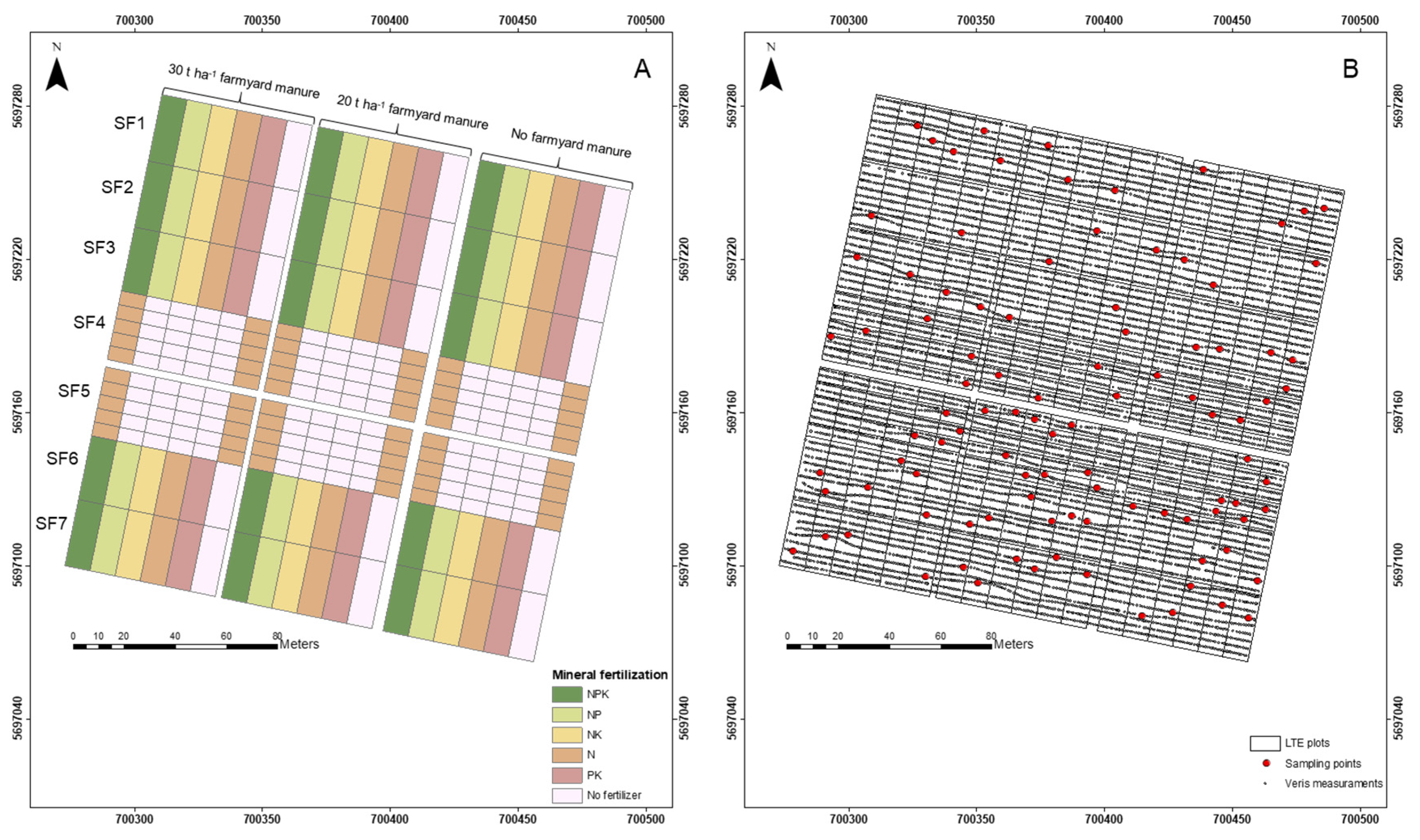
Figure 2.
Two-step model training and evaluation procedure. Step 1: regression model training (R-model), Step 2: ordinary kriging (K-model). X= spectra, Y= SOC values, RMSER= RMSE of the regression model, RMSER+K = RMSE of the R+K modeling approach.
Figure 2.
Two-step model training and evaluation procedure. Step 1: regression model training (R-model), Step 2: ordinary kriging (K-model). X= spectra, Y= SOC values, RMSER= RMSE of the regression model, RMSER+K = RMSE of the R+K modeling approach.
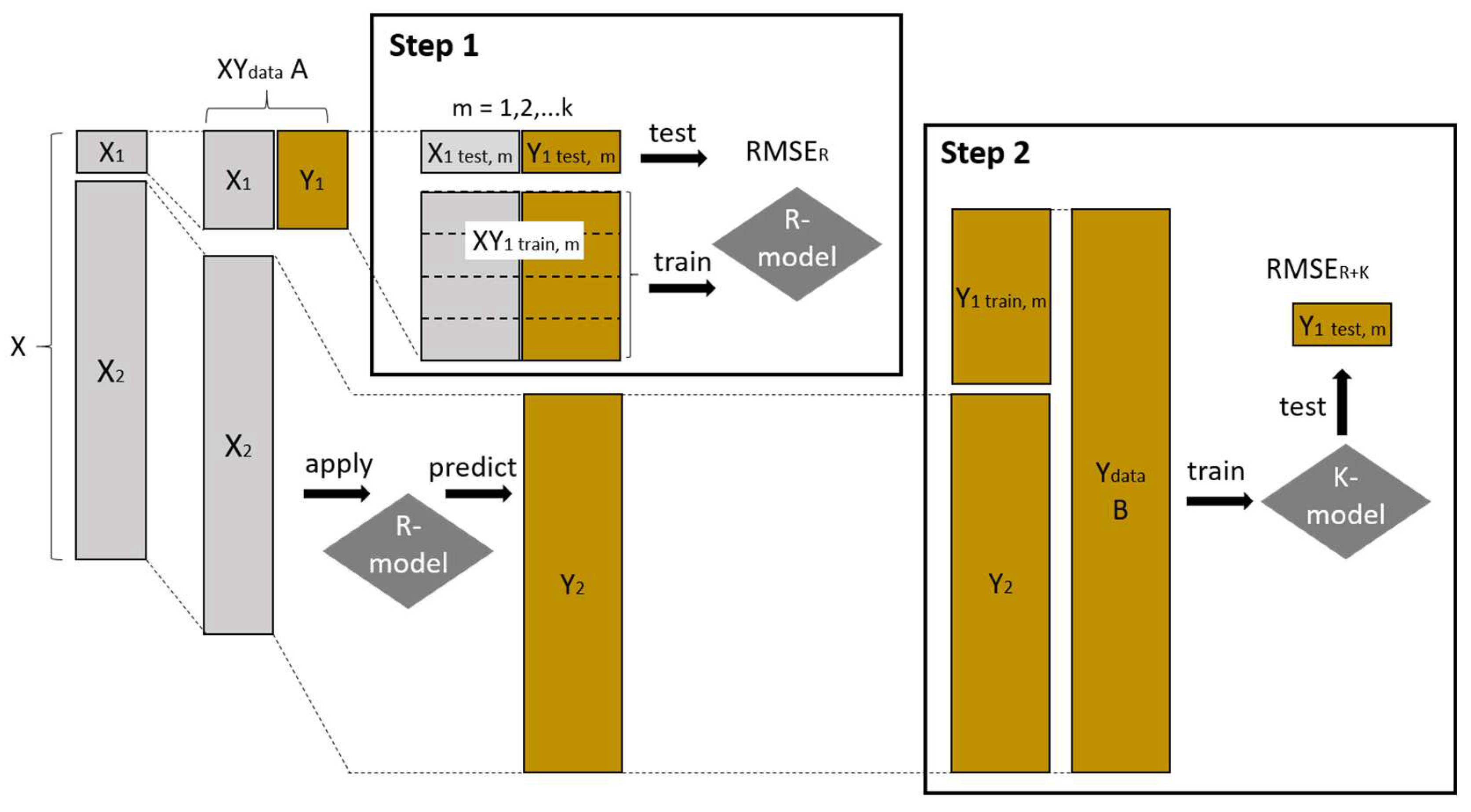
Figure 3.
Boxplots of the optimal number of PLSR components of the 25 models trained with data preprocessed by SG: Saviztky Golay, SGCR: Saviztky Golay + continuum removal, gapDer: gap segment algorithm, and MSC: multiplicative scatter correction.
Figure 3.
Boxplots of the optimal number of PLSR components of the 25 models trained with data preprocessed by SG: Saviztky Golay, SGCR: Saviztky Golay + continuum removal, gapDer: gap segment algorithm, and MSC: multiplicative scatter correction.
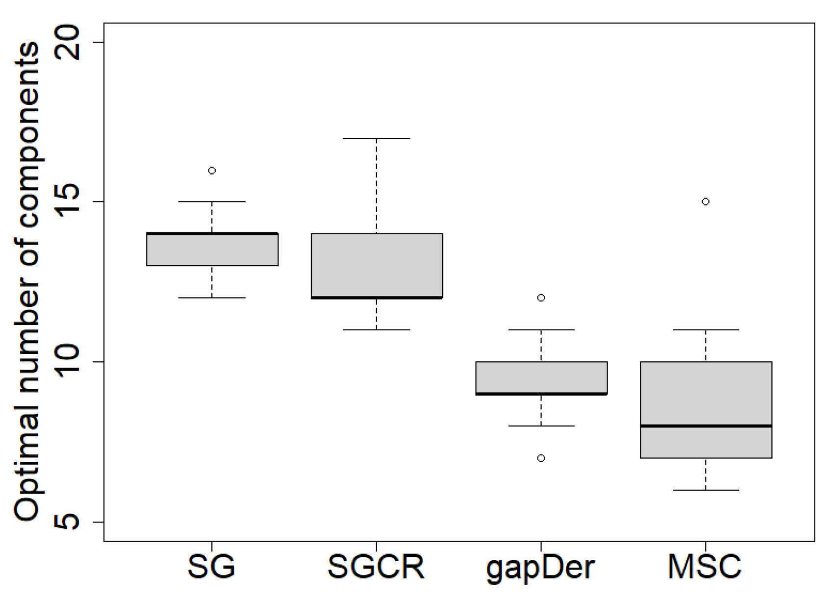
Figure 4.
Semivariogram models corresponding to the PLSR predicted SOC of the on-the-go spectral data using the 25 models. The semivariogram model lines correspond to the average values, while the boxplots show the variation of the parameter values. (A) SG: Savitzky-Golay, (B) SGCR: Savitzky-Golay + continuum removal, (C) gapDer: gap segment algorithm, and (D) MSC: multiplicative scatter correction. SPH: Spherical, EXP: Exponential, GAU: Gaussian.
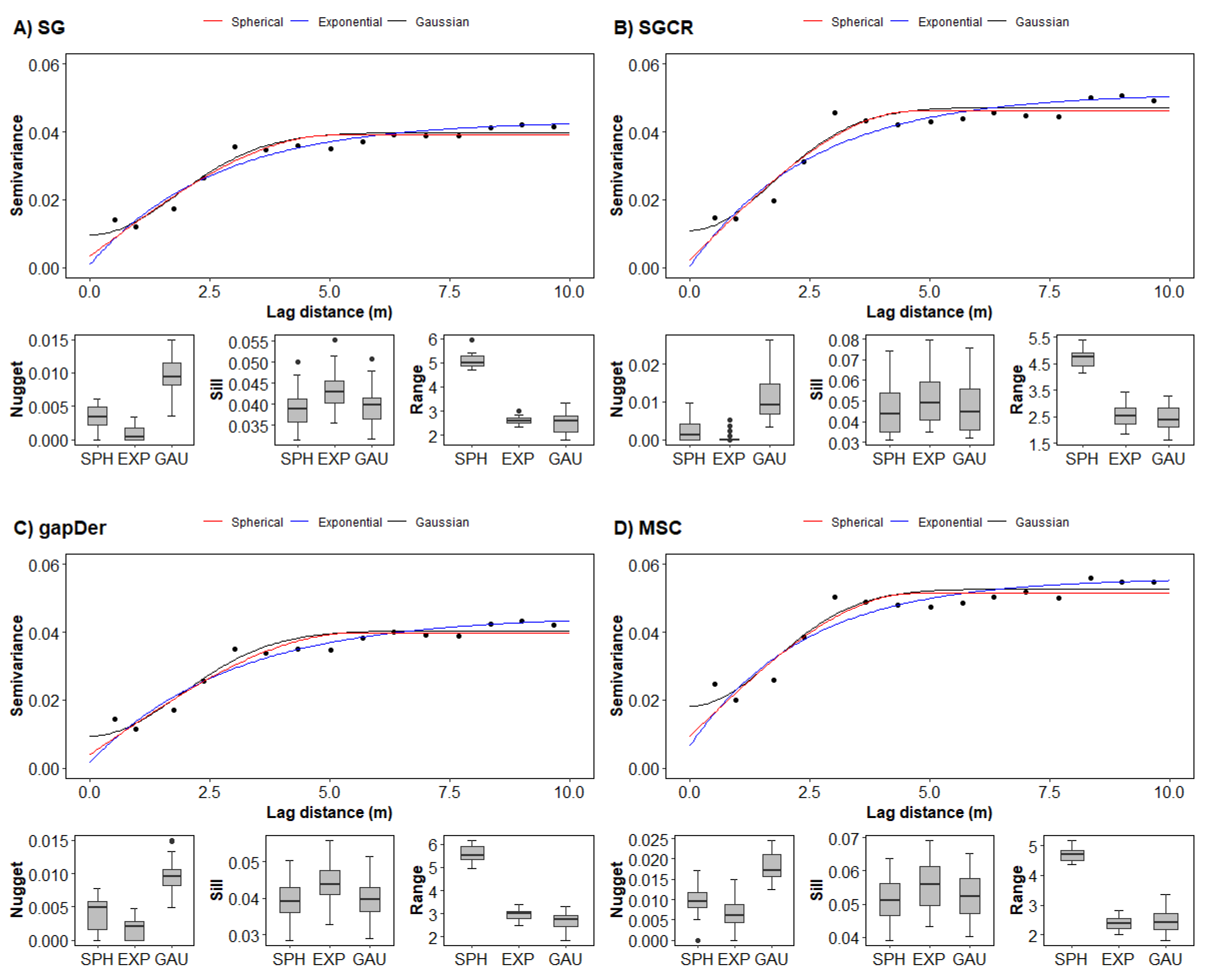
Figure 5.
Predictive model performance of Step 1 for each preprocessing method (5 values per boxplot). SG: Saviztky Golay, SGCR: Saviztky Golay + continuum removal, gapDer: gap segment algorithm, MSC: multiplicative scatter correction.
Figure 5.
Predictive model performance of Step 1 for each preprocessing method (5 values per boxplot). SG: Saviztky Golay, SGCR: Saviztky Golay + continuum removal, gapDer: gap segment algorithm, MSC: multiplicative scatter correction.
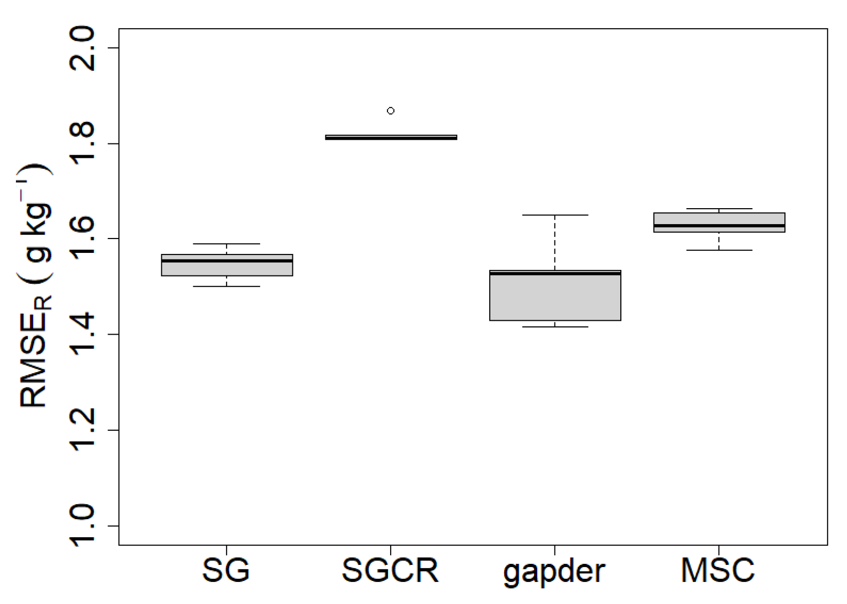
Figure 6.
Predicted versus observed values of modeling Step 1, with 5 predictions per sampling location. A) SG: Saviztky Golay, B) SGCR: Saviztky Golay + continuum removal, C) gapDer: gap segment algorithm, D) MSC: multiplicative scatter correction.
Figure 6.
Predicted versus observed values of modeling Step 1, with 5 predictions per sampling location. A) SG: Saviztky Golay, B) SGCR: Saviztky Golay + continuum removal, C) gapDer: gap segment algorithm, D) MSC: multiplicative scatter correction.
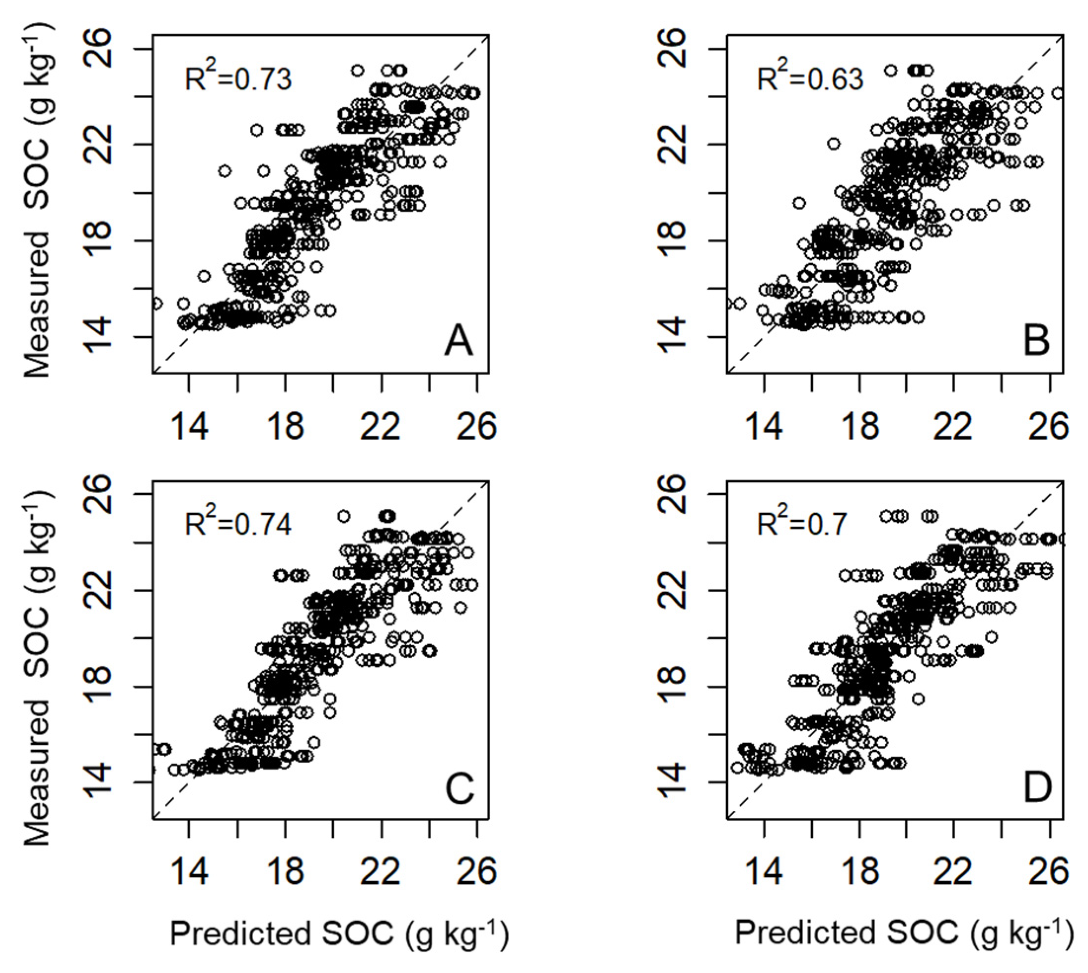
Figure 7.
Overall predictive model performance (Step 1 + Step 2) for each preprocessing method and each semivariogram model. Dashed lines represent the median value obtained in Step 1. SG: Saviztky Golay, SGCR: Saviztky Golay + continuum removal, gapDer: gap segment algorithm, MSC: multiplicative scatter correction, SPH: Spherical, EXP: Exponential, GAU: Gaussian.
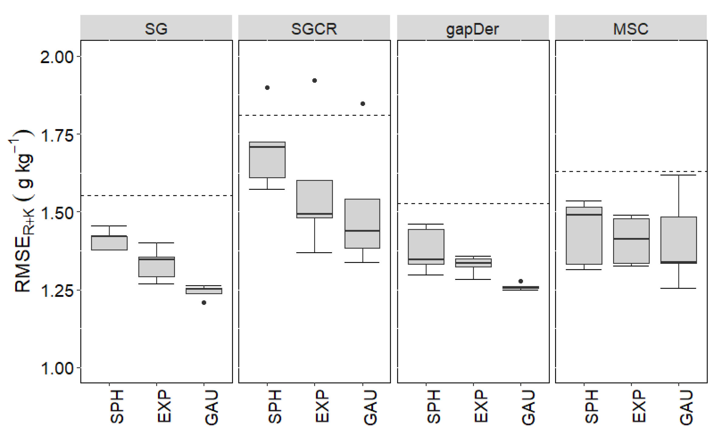
Figure 8.
Predicted versus observed values of the overall modeling procedure (Step 1 + Step 2) with five predictions per sampling location. SG: Saviztky Golay, SGCR: Saviztky Golay + continuum removal, gapDer: gap segment algorithm, MSC: multiplicative scatter correction.
Figure 8.
Predicted versus observed values of the overall modeling procedure (Step 1 + Step 2) with five predictions per sampling location. SG: Saviztky Golay, SGCR: Saviztky Golay + continuum removal, gapDer: gap segment algorithm, MSC: multiplicative scatter correction.
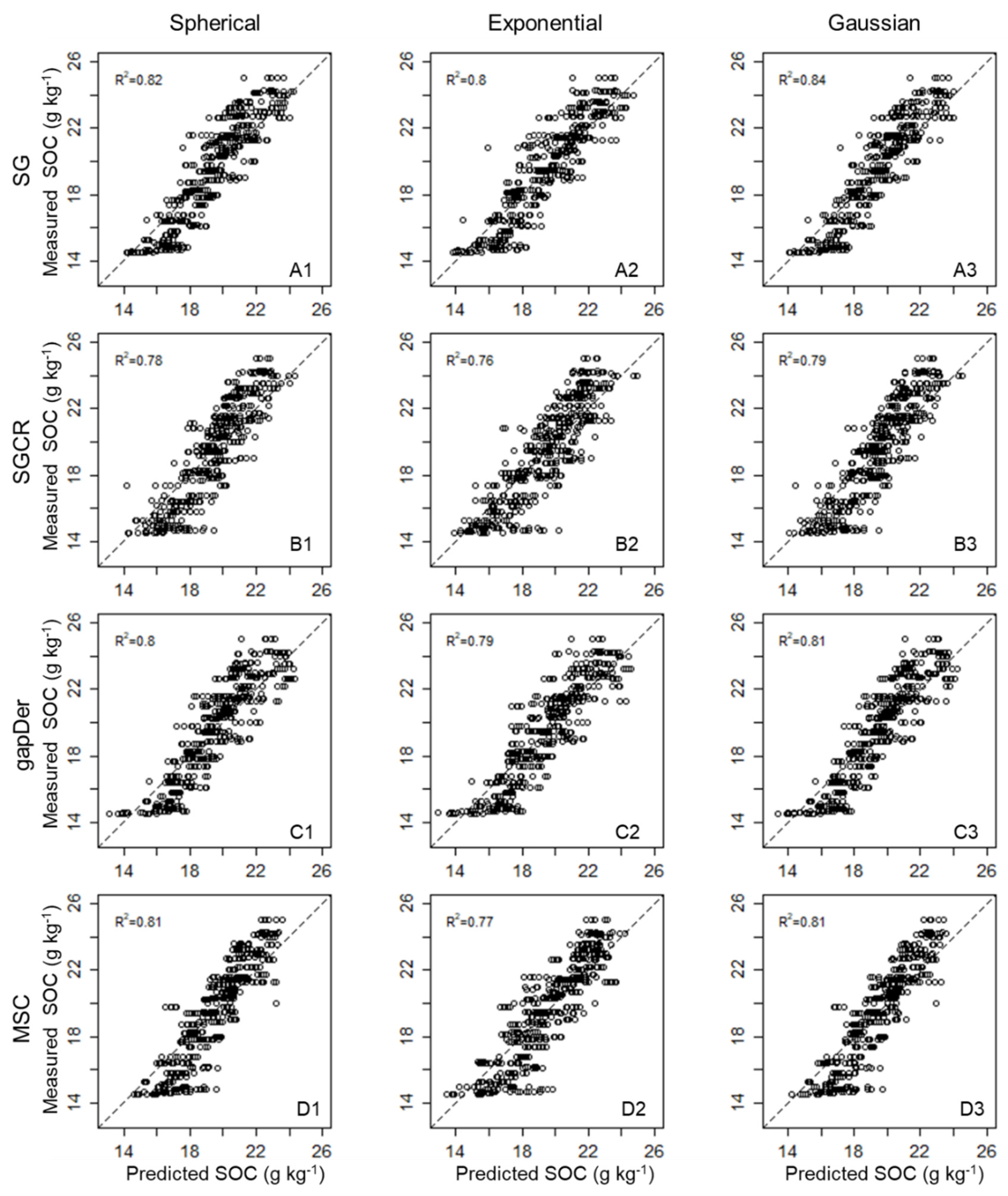
Figure 9.
Average residuals of predicted SOC values per sampling point location of A) Saviztky Golay-Gaussian, and B) gap segment algorithm-Gaussian methods.
Figure 9.
Average residuals of predicted SOC values per sampling point location of A) Saviztky Golay-Gaussian, and B) gap segment algorithm-Gaussian methods.
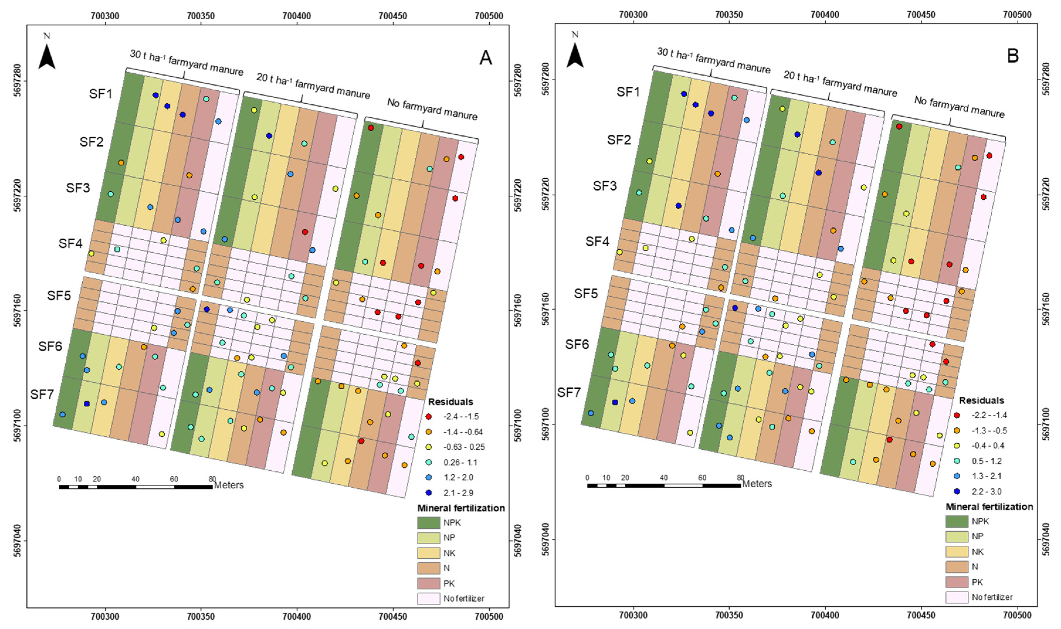
Figure 10.
The median of predicted SOC values of the R+K models with the best performance. A) Saviztky Golay-Gaussian, B) gap segment algorithm-Gaussian, C) difference between models.
Figure 10.
The median of predicted SOC values of the R+K models with the best performance. A) Saviztky Golay-Gaussian, B) gap segment algorithm-Gaussian, C) difference between models.
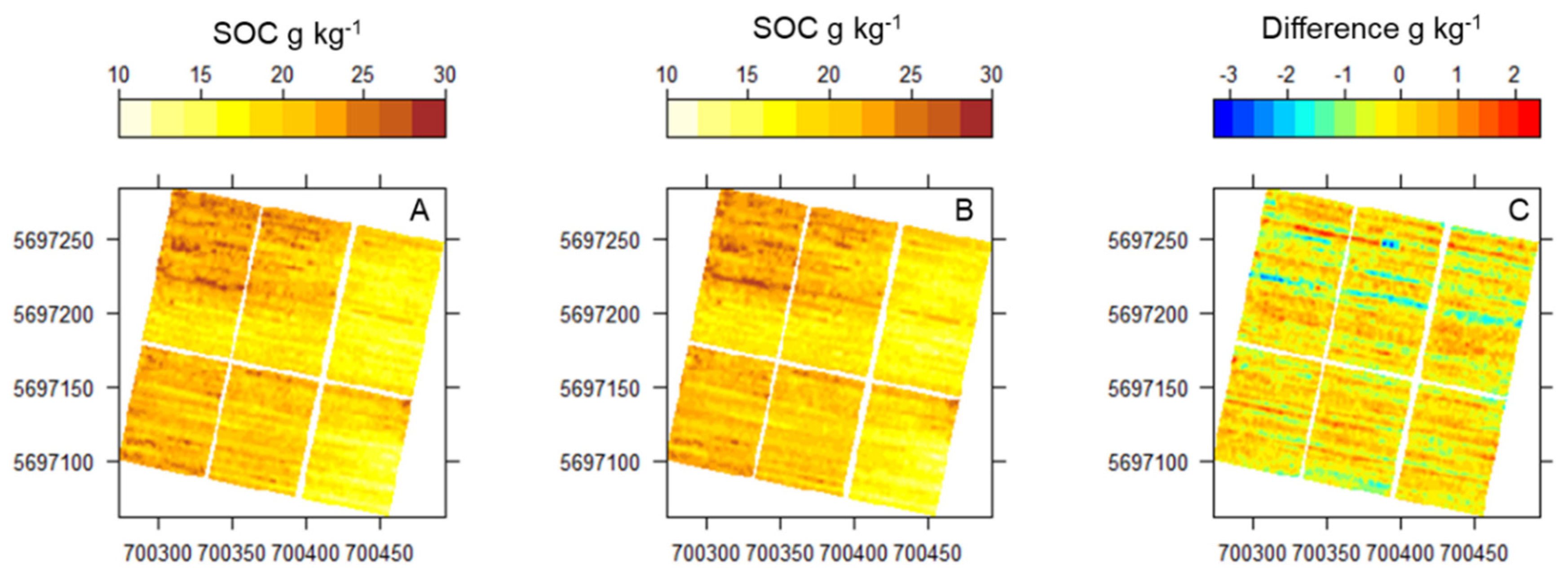
Figure 11.
Interquartile range (IQ) of predicted SOC values of models with the best performance and the difference between predictions. A) Saviztky Golay-Gaussian, B) gap segment algorithm-Gaussian, C) difference between models.
Figure 11.
Interquartile range (IQ) of predicted SOC values of models with the best performance and the difference between predictions. A) Saviztky Golay-Gaussian, B) gap segment algorithm-Gaussian, C) difference between models.
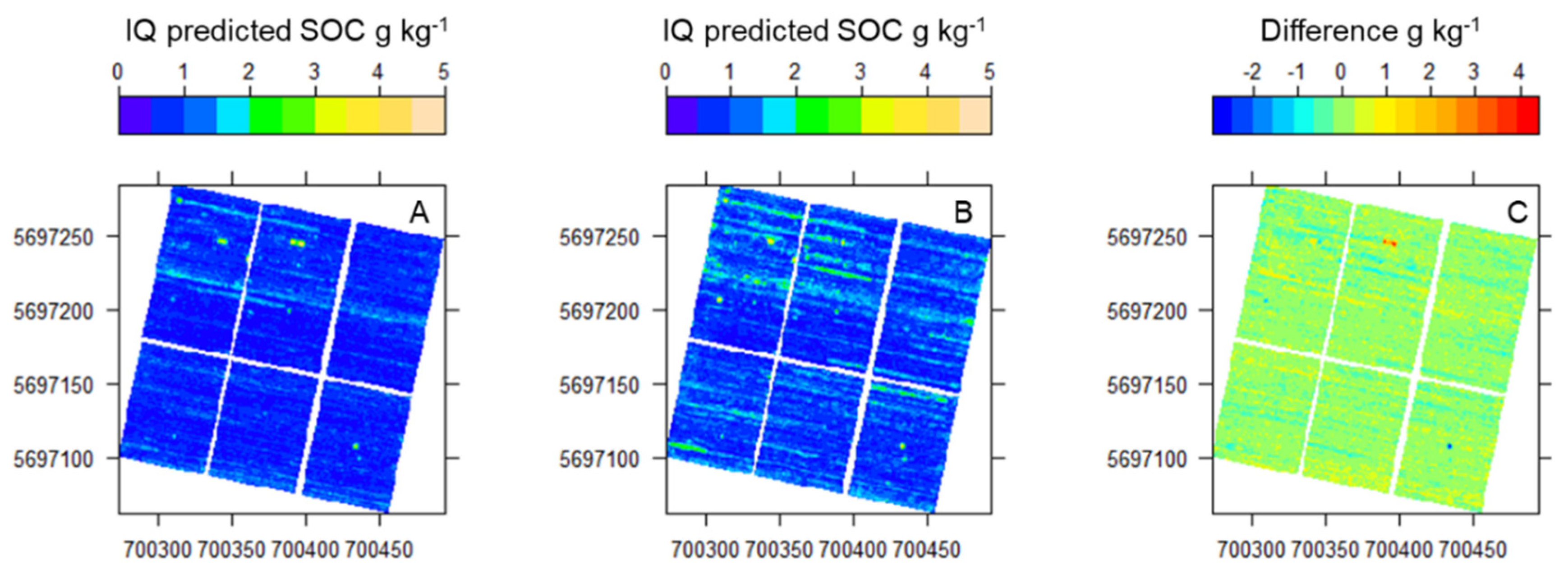
Figure 12.
Maps of the median of predicted SOC values using the Saviztky Golay-Gaussian method using 3 different approaches, A) pairing points of Veris data, B) extending the maximum spatial separation distance for the semivariogram to 25 m, C) applying block kriging with the field plots as block delineation.


Table 1.
Combinations of preprocessing techniques used in this study; w is window size, s segment size.
Table 1.
Combinations of preprocessing techniques used in this study; w is window size, s segment size.
| Preprocessing method | Abbreviation | Veris wavelength range |
|---|---|---|
| Savitsky-Golay | SG | 432-2201 |
| Saviztky-Golay w=11 and continuum removal | SGCR | 432-2201 |
| Gap segment algorithm (w=11, s=10) | gapDer | 408-2186 |
| Multiplicative scatter correction | MSC | 403-2201 |
Disclaimer/Publisher’s Note: The statements, opinions and data contained in all publications are solely those of the individual author(s) and contributor(s) and not of MDPI and/or the editor(s). MDPI and/or the editor(s) disclaim responsibility for any injury to people or property resulting from any ideas, methods, instructions or products referred to in the content. |
© 2023 by the authors. Licensee MDPI, Basel, Switzerland. This article is an open access article distributed under the terms and conditions of the Creative Commons Attribution (CC BY) license (https://creativecommons.org/licenses/by/4.0/).
Copyright: This open access article is published under a Creative Commons CC BY 4.0 license, which permit the free download, distribution, and reuse, provided that the author and preprint are cited in any reuse.


