
Submitted:
16 April 2025
Posted:
18 April 2025
You are already at the latest version
Abstract
In Eritrea, conventional agriculture is the main stay for most of the population for livelihood where crop productivity is very low, and food insecurity and poverty are common. Though initiatives are being taken to promote the agricultural sector in the country, soil resources are not addressed. Soil studies are very limited, and the country lacks digital soil mapping. Thus, the study aims to develop robust soil organic carbon (SOC) prediction model/s for the western lowland soils where most of the agricultural activities of the country are carried out. We employed MLR, PLS, Cubist, RF, GB and XGB algorisms, and regressed multiple soil, climatic, Landsat 8 (L8) bands and spectral indices against SOC (n=178) through machine learning. The SOC modelling was done in 3 steps with 25, 14, and 06 independent environmental variables to identify the main SOC driver variables. Models performances were evaluated using the RMSE, R2, and RPD metrics. The SOC content in the study area was low with an average of 0.44%, which needs effective soil carbon improvement planning. The accuracies of all the tested models were good enough in all the three steps. The PLS model with 14 input variables gave the highest accuracy (RMSE = 0.1128%, R2 = 0.8268, RPD = 2.4393), and RF model with 06 input variables recorded the lowest (0.1435%, 0.7032, 1.9173). MLR and XGB models improved but GB model worsened with dimensionality reduction. PLS, Cubist, and RF models gave better results with 14 input variables. According to the RPD category, the PLS, XGB, and Cubist models were very good, and RF was good in all the three steps. MLR improved from good to very good but GB deteriorated from very good to good. Rainfall was the most important variable for SOC spatial variability prediction in the study area. Temperature, Green and SWIR2 Landsat 8 bands, NDSI, BR2, Sand, and MSAVI2 also had good capacity to predict the SOC spatial variability. We conclude that all the developed models have good predictive accuracies to be employed in short-mid-long-term planning and monitoring of soil fertility and productivity improvements, ecosystem restoration, and climate-change mitigation action. The study, being the first of its kind in the country, has laid the foundation for digital soil mapping (DSM) and management in the country, and more detailed SOC modelling studies are advised with more soil samples in the study area and other parts of the country for better results.
Keywords:
conventional agriculture
; sustainable agriculture
; SOC modelling
; machine learning
; variables dimension reduction
; rainfall
; Landsat 8 bands
; NDSI
; BR2
; MSAVI2
1. Introduction
SOC has the potential to save the world [1] as it is the key factor in the global carbon (C) cycle. If it is enhanced, it improves soil health and fertility, microbial diversity and activity, nutrient cycling, soil water retention, restores degraded ecosystems, and mitigates climate change [1,2]. Many of the SDGs can be achieved through proper management of soil resources: for example no poverty (1), no hunger (2), climate change (13), and life on land (15). Soil is the largest terrestrial carbon (C) bank. It contains approximately 2500 Gt C stock (1550 Gt organic and 950 Gt inorganic) in the first 1 m depth [3]. However, soils have been unwisely exploited to the maximum. Agricultural expansions, for example, have swallowed vast natural forestlands, and consequently, reduced SOC stock and increased atmospheric CO2 [4,5,6], and such emissions share 25–30% of the total global greenhouse gas emissions [7]. Sadly, soils have lost 116 Gt C due to land cultivation [8]. Conventional and chemical fertilizer based intensive farming practices have led to different challenges like food insecurity, deforestation, land degradation, drought, desertification, climate change, etc. The key to resolve these issues is shifting to sustainable agriculture, which has the potential to eradicate hunger and poverty, enhance natural resources and mitigate climate change, and ensure sustainable development.
Likewise, Eritrea faces widespread land degradation, soil erosion, soil fertility decline, food insecurity, poverty, drought, desertification, and climate change [9,10,11,12,13]. Eritrea is located in the Sahel region where rain-fed agriculture is difficult. Though about 72% of the country is semi-desert and arid, more than 75% of the population depends on mixed (crop and livestock) subsistence rain-fed farming for its livelihood. Crop productivity is very low; less than 0.7 t ha-1 [14]. Total crop failures and mass livestock deaths are common due to recurrent droughts after 3-4 years. To tackle these problems, and promote sustainable agriculture, natural resources and sustainable development, the country plans and runs massive soil and water conservation campaigns through mass mobilization. In the recent years, in many parts of the country, a considerable number of micro and macro dams are constructed, and good amount of water is conserved in these structures. Among the macro dams are Kerkebet, Gahtelai, Misilam, Logo, Gerset, Fanco-Rawi, Bademit, and Fanco-Tsimu with the capacities of 330, 50, 35, 31, 20, 20, 17, and 14 million m3 water, respectively. As a result, the number of down dam irrigated farms is growing. Though moisture stress is being addressed, soil management and soil fertility problems remain unattended. Soil management is poor and soil studies are very limited in the country. The very limited soil studies are also based on traditional soil sampling and laboratory analysis, which is destructive to the soil structure, labour-intensive, time-consuming, expensive, environmentally unsafe, and they don’t provide continuous and complete information of the entire target area [15,16].
The advancements in remote sensing, GIS, and machine learning (ML) provide and enable us process, assess, model, and interpret huge environmental data for better understanding, developing management and monitoring plans of resources [17]. Poor countries like Eritrea need to tap these legacies for efficient resources management for their sustainable development. In Eritrea, digital resources management is very poor, and especially in soil resources. The country lacks DSM though complex soil-landscape relationships, and soil properties including SOC can be modelled and predicted with good accuracy using environmental data through ML [18] with no/little cost. Thus, the study aimed to develop SOC predictor model/s for the western lowlands soils of the country where most of the agricultural activities are carried out. We employed multiple soil, climate, Landsat 8 bands, and spectral indices as input variables, and multiple linear regression (MLR), partial least squares (PLS), Cubist, random forest (RF), gradient boosting (GB), and extreme gradient boosting (XGB) algorisms through machine learning. The study could help for developing effective short-mid-long-term management and monitoring plans for continuous improvements in soil health, food production, ecosystem restoration and climate change mitigation actions.
2. Materials and Methods
2.1. Study Area
The study was conducted in the western lowlands of Eritrea (Figure 1), which is located within the Gash Barka administrative zone. The administrative zone borders with the western escarpments of the country to the east, Sudan to the west and north, and Ethiopia to the south. The Gash Barka administrative zone is further divided in to 16 subzones namely Laelay Gash, Goluj, Teseney, Haykota, Gogne, Barentu, Shambuqo, Molqi, Logo Anseba, Mensura, Mogolo, Aqrdet, Dge, Forto, Kerkebet, and Sel’a subzones. The study did not include the Sel’a subzone (at the north) due to lack of soil data, and Mensura, Logo Anseba, and Molqi subzones, and part of Shambuqo subzone (all at the east) due to lack of soil data for these places. Its climate is dominantly arid [19]. In the study area, the mean monthly temperature, and annual rainfall range from 23.7 to 29.4 oC, and 184 to 680 mm, respectively [20]. Temperature increases from south to north, and rainfall does the opposite (Figure 2). The topography is mostly lowland plains with deep soils. Elevation decreases from south to north, and from east to west (Figure 1). Most of the area lays between 400 to 800 m above mean sea level.
The study area has vast arable lands, and a number of crossing through seasonal rivers mainly the Gash, Barka, and Anseba Rivers and their tributaries. It also has one perennial river, the Setit River (at the border with Ethiopia). The study area exercises extensive conventional farming in which mixed crop-livestock and agro-pastoral (in most parts), and pastoral (mostly in the northern part) practices are dominant. Sorghum is dominantly grown in the area, which covers 72.26%, followed by pearl millet (12.52%), sesame (8.33%), finger millet (1.68%), etc. The soils have been conventionally cultivated and grazed for hundreds of years. The soils comprise of fluvisols, leptosols, lixisols, and vertisols, and in small amount cambisols. They are cultivated during the rainy season, grazed heavily after harvesting, and stay bare for most of the year. As a result, crop productivity is very poor; 30 years (1992-2021) records of crop production of the ministry of agriculture show that the average productivity, in t ha-1, of sorghum = 0.52, pearl millet = 0.32 and sesame = 0.33. Total crop failures and mass livestock deaths are also common every 3-4 years due to frequent droughts. Livestock rearing is very popular there where herds of animals overgraze and degrade lands, and move freely from place to place in search of grass and water. Herds of camels, cattle, sheep, and goats are very common.
The area is home to variety of tree species like different acacia species, Hyphaene thebaica, Adansonia digitata, Balanites aegyptiaca, Tamarindus indica, Ziziphus spina-Christi, etc. Riverine forests (mainly Hyphaene thebaica) are common along the river banks. It is also home to different wildlife animals like elephants, antelopes, dorcas gazelles, baboons, v vet monkeys, hyenas, warthogs, ostriches, ibex, foxes, honey badges, bushbucks, and a wide range of birds and reptiles [21]. However, this biodiversity is diminishing from time to time due to deforestation, agricultural expansion, drought, etc. Most of the study area is left with bare soils or scattered acacia trees and shrubs, especially the western, middle and northern parts. The NDVI (Figure 2) of the area also shows that it has almost no vegetation cover except the southern part and riverine areas where some vegetation is present.
Recently, different micro and macro dams are built in the area, and water is stored for different purposes; irrigation and agroindustry, livestock, wildlife, household, etc. Irrigated agriculture and agroindustry is planned in the area, and different small and largescale farms are initiated. Some of the largescale farms that are included in the study are the Kerkebet, Afhimbol, Gerset, and Fanco farms.
2.2. Soil and Climatic Data
As there were not any previous SOC modelling studies neither in the study area nor in the country, we proposed different soil, climatic, Landsat 8 (L8) bands, and spectral indices as input variables to predict the spatial distribution of SOC in the study area. Topographic variables were not included due to the flat-dominated topographic nature of the study area, which is lowland. Table 1 displays the proposed potential SOC predictor variables, their resolutions and sources.
The study collected 92 georeferenced composite surface (0-30 cm) soil samples from September to November 2023 using 30 cm deep auger adopting systematic sampling technique. To make a composite soil sample, 5 individual subsamples were collected within a 10 m radius, and mixed well. Latitude and longitude coordinates were recorded at the center. The soil samples were dried, grounded, and sieved following standard procedures. They were analyzed in the soil laboratory of National Agricultural Research Institute (NARI), Eritrea, for SOC using the [22] wet oxidation method after modified by [23], pH (pH meter) [24], electrical conductivity (EC meter) [25], particle size distribution (hydrometer) [26]. Additionally, the study collected legacy soil data from the soil laboratory of NARI, which raised the total SOC dataset to 178 along with their respective clay, silt, sand, texture, pH, and EC value, and latitude and longitude coordinates. We extracted mean annual rainfall and monthly temperature data from the WorldClim 2.1 (30 seconds) [20] at https://www.worldclim.org/data/worldclim21.html#.
2.3. Landsat 8 and Spectral Indices Data
The study downloaded four L8 images with (path, row, dated) of (170, 049, 17/04/2024), (170, 050, 29/02/2024), (171, 049, 08/04/2024), and (171, 050, 08/04/2024) form the USGS archives https://earthexplorer.usgs.gov/ accessed on 24 March 2025. We chose images with < 10% cloud cover in the dry months February to April to avoid the interferences of clouds and seasonal vegetation. We computed different spectral indices using their respective formula (Table 2) using raster calculator in QGIS 3.38. These spectral indices were normalized difference vegetation index (NDVI), green NDVI (GNDVI), enhanced vegetation index 2 (EVI2), infrared percentage vegetation index (IPVI), soil adjusted vegetation index (SAVI), Optimized SAVI (OSAVI), modified SAVI2 (MSAVI2), normalized difference water index (NDWI) for vegetation water content, normalized difference soil index (NDSI), bare soil index (BSI), hyperspectral BSI (HBSI), soil organic carbon index (SOCI), normalized difference moisture index (NDMI), burn ration (BR), BR2, colouration index (CI), hue index (HI), and brightness index (BI). Different studies employed these spectral indices in different combinations [27,28,29,30]. L8 bands B1 to B7; Blue, Green, Red, near infrared (NIR), shortwave infrared 1, and 2 (SWIR1, and SWIR2) [17,27,31] were also included in the dataset as potential SOC predictors (Table 1).
2.4. Selection of Input Variables
The dataset was composed of 33 independent input variables and one dependent target variable (SOC). Using a large number of variables in prediction modelling may also lead to wrong conclusions due to multicollinearity effects between some of the independent variables and/or due to the effects of the variables that have very weak correlation with the target variable. It is advisable to analyze the relationships between the input variables, as well as the target variable for sound selection of input variables for effective modelling. Thus, we decided to follow 3 steps of reduction of dimensionality, and run SOC prediction modelling in each step so that to compare the results obtained through different numbers of input variables.
Step 1. Based on Spearman rank correlation, from each set of the variables that were perfectly correlated (1.0**) with each other or among them, we retained one variable from each set and omitted the others. We also removed the variables that had no significant correlation with SOC (p > 0.05).
Step 2. From each set of the variables that were very highly correlated (> = 0.9**) with each other or among them, we omitted the variable/s with weaker correlation/s with SOC by keeping the one with highest correlation [30].
Step 3. From each set of the variables that had high correlation (>=0.7**) with each other or among them, we omitted the variable/s with weaker correlation/s with SOC by keeping the one with highest correlation. Moreover, we removed the variables that had weak correlation (< 0.3**) with SOC.
2.5. Models Training, Calibration, Prediction and Evaluation
Figure 3 displays the whole conceptual flowchart of the methodologies used here. The training and calibration of the models was on the basis of the extraction of the independent proposed SOC predictor variables to the target SOC values. We employed python 3.11.7 in the Jupiter notebook environment to run the modelling. The dataset was randomly divided into training (80%) and testing (20%). We tested MLR, PLS, Cubist, RF, GB, and XGB algorisms, and the 10-fold cross validation grid search technique was used to find the best model fit in each algorism. Models were fitted, trained, calibrated, and finally predictions were made. Performances of models were evaluated using RMSE, R2, and RPD [18,47], which are given by the equations (1), (2), and (3).
Where; SSres = ∑ (yi − ýi)2 (residual sum of squares), SStot = ∑(yi - yˉ)2 (total sum of squares), yi = observed values, ýi = predicted values, and yˉ = mean of observed values, n = number of observations, SD = standard deviation of observed values
Furthermore, models are categorized as per their RPD values as; very poor (RPD< 1), poor (1-1.4), fair (1.4-1.8), good (1.8-2.0), very good (2.0-2.5), and excellent (>2.5) [47]. RPD is the factor by which the prediction accuracy has been increased compared to using the mean of the original data.
3. Results and Discussions
3.1. Statistical Analysis of Observed Soil Properties
The studied soils had moderate clay and silt, and high sand contents with averages of, in %, 27.27, 29.51, and 43.48, respectively (Table 3). They showed high spatial variation within the study area with CV values of, in %, 51.23, 39.36, and 41.65, respectively. The soils were none-saline but moderately alkaline. Very few strongly alkaline soils were also observed around Adi Hakin, Tekombia, Fanco, Mogolo, and Kerkebet. The alkalinity is may be attributed to the calcareous nature of arid region soils [48] in which calcium carbonate test is helpful for better managerial actions. Attention is also needed that manganese, copper, zinc, and boron may be deficient in alkaline soils [49]
The soils had poor SOC content. It ranged from, in %, 0.02 to 1.01 (Table 3, Figure 4) with a mean = 0.44, SD = 0.28, and CV = 62.89% (Table 3). [11,12,13] also reported low SOC contents at other parts of the country. Conventional tillage practices, continuous mono-cropping, heavy crop residue harvest, almost no addition of organic matter, overgrazing, soil erosion, among others, might have contributed to the low SOC contents. SOC decreased from south towards north in the same manner as the rainfall, and inversely as temperature in the study area do. This indicates that climate may have great influence on the spatial distribution of SOC in the study area. Subzone Laelay Gash (southern part) recorded the highest average SOC, and subzone Kerkebet (northern part) the lowest (Figure 4).
In the study area, SOC can be improved through good agronomic practices like crop rotation, legume-cereal intercropping, crop residue retention, cover cropping, agroforestry practices, farmyard manure application, and integrated and diverse cropping/farming systems, no/minimal tillage, incorporating biochar or organic amendments. Organic amendments are very important to improve conditions of soils where natural vegetation is scarce like the study area. Two abundant organic sources remained untapped in the study area and the country; Prosopis juliflora and organic municipal waste. By channeling these resources to the farming system, the benefit will not only be on food production, but ecological, socio-economic, health, environmental, etc. benefits. Thus, composting and biochar technologies can be promoted along with research experiments.
As the study area is stressed with overgrazing, handling right stocking rate, rotational grazing, giving enough rest periods for pastures, establishing enclosures and promoting cut and carry methods, reseeding with legumes, and developing and using grazing and SOC dynamics models [4,50] could improve the health and fertility of the soils.

Table 3.
Statistical analysis of observed soil properties (n = 178).
| Parameter | Minimum | Maximum | Mean | *Status | SD | CV, % |
|---|---|---|---|---|---|---|
| Sand, % | 2.80 | 85.10 | 43.48 | High | 18.11 | 41.65 |
| Clay, % | 3.50 | 57.30 | 27.27 | Moderate | 13.97 | 51.23 |
| Silt, % | 7.50 | 59.00 | 29.51 | Moderate | 11.61 | 39.36 |
| EC, dS m-1 | 0.01 | 1.92 | 0.19 | Non-saline | 0.28 | 142.03 |
| pH | 6.80 | 9.83 | 8.22 | Moderately alkaline | 0.54 | 6.59 |
| SOC, % | 0.02 | 1.01 | 0.44 | Poor | 0.28 | 62.89 |
3.2. Correlation Analysis, and Variables Dimension Reduction
The Spearman correlation analysis showed that most of the input variables had high correlation with SOC. Rainfall got the highest correlation (0.779**) with SOC followed by Temperature (-0.774**), Green, BI, Blue, Red, B1, SOCI, NIR, NDVI (0.618**), etc. However, 5 variables namely pH, CI, HI, BR, and HBSI failed to fulfil the significant level (p>= 0.05) of correlation with SOC, and were removed from the input dataset.
Perfect correlations (1.0**) were observed between different groups of input variables (NDVI and IPVI), (SAVI and EVI2), (NDWI and GNDVI). Thus, NDVI, SAVI, and NDWI were retained, and the other 3 variables were removed from the dataset at the beginning. Many independent variables had also very high correlations (>=0.9**) between each other. Temperature and Rainfall showed very high correlation (-0.974**) between each other. Very high correlations were also observed among these groups (B1, Blue, Green, Red, NIR, BI, and SOCI), (NDVI, SAVI, and OSAVI), (NDSI and NDWI), and (SWIR1 and SWIR2). According to their correlation with SOC, Rainfall, Green, NDVI, NDSI, and SWIR2 were retained but the other 11 variables were omitted from the dataset at Step 2.
High correlations (>=0.7**) were also observed between different groups of the independent variables; (Rainfall, NDVI, and Green), (Sand, Clay, and Texture), and (NDSI, and NDMI). Accordingly, Rainfall, Sand, and NDSI were retained, and the others removed. Variables with weak correlations (<0.3**) with SOC were also removed at this step; Silt, EC, and BSI. At the end, the dataset remained with 06 input variables namely Rainfall, MSAVI2, Sand, NDSI, BR2, and SWIR2. Thus, the SOC modelling was executed in 3 steps with 25, 14, and 06 groups of input variables, respectively.
3.3. SOC Prediction Accuracy of Models
The spatial distribution of SOC in the study area was predicted with good accuracies with all the tested models in all the variables dimension reduction steps. Responses of models to dimensionality reduction varied (Table 4). MLR and XGB showed continuous improvement, 6.65% and 3.74%, respectively, but GB worsened, 9.97%, with dimensionality reduction. The rest three models (PLS, Cubist and RF) improved in the second step but worsened at the end (Table 4). The highest model accuracy was recorded with PLS model with (RMSE = 0.113%, R2 = 0.827, RPD = 2.439) with 14 input variables, and the lowest was in RF model (0.144%, 0.703, 1.917) with 06 input variables.
In the first step, which involved 25 input variables, the PLS model with (RMSE = 0.128%, R2 = 0.776, RPD = 2.147) yielded the highest accuracy followed by XGB and GB, respectively. MLR model with (0.143%, 0.737, 1.925) recorded the lowest model accuracy among the tested models (Table 4) at the first stage. At the second step, with 14 variables, all the models except GB showed improvements; for example 11.94%, and 7.09% in PLS, and Cubist models, respectively. At this stage, the PLS model (RMSE = 0.113%, R2 = 0.827, RPD = 2.439) outperformed the others followed by Cubist. At the final step, with 06 input variables, the XGB model with (RMSE = 0.124%, R2 = 0.792, RPD = 2.224) resulted the highest predictive accuracy followed by PLS (0.131%, 0.767, 2.104), and MLR (0.133%, 0.758, 2.062), respectively (Table 4). Comparatively, the PLS, Cubist, and RF models gave better results with 14 input variables, XGB and MLR models with 06, and GB model with 25 input variables.
According to the RPD value based category of models, the PLS, Cubist and XGB models were within the very good category in all the three steps. The MLR model improved from good at the first steps to very good at the two followed steps (Table 4). However, GB model reduced form very good in the first two steps to good at the last stage. RF model was good in all the stages. The accuracies of all the tested models in all stages are to the average of most of DSM and SOC prediction modelling reports [18,52,53,54], and are good enough to be employed for SOC improvement planning and monitoring in the study area and areas with related conditions.
Figure 5.
Predicted SOC by PLS, Cubist, and MLR models with 14, 14, and 06 input variables, respectivel.
Figure 5.
Predicted SOC by PLS, Cubist, and MLR models with 14, 14, and 06 input variables, respectivel.
3.4. Importance of Variables
The display of variables importance by the RF model showed more consistency through all the three steps than XGB, and GB models. It was also more consistent to the Spearman correlation analysis of the independent variables with SOC. Thus, importance of variables is discussed here according to the RF model.
According to the RF model, at the first step (with 25 variables), the first top ten important variables for SOC prediction in the study area were Rainfall, Temperature, B1, SOCI, BI, Green, Red, NIR, Blue, and NDSI, respectively (Figure 6), and they addressed 77.67% of the SOC spatial variation in the study area. Moreover, the first five variables explained 57.63% of the SOC distribution. In the second step (with 14 variables), the first top five and ten important variables addressed 62.86%, and 89.94% of the SOC variability, respectively. They were Rainfall, Green, NDSI, NDVI, SWIR2, BR2, NDMI, Sand, MSAVI2, and Clay, respectively. In the final stage (with 06 input variables), the importance of variables was ordered as Rainfall, NDSI, SWIR2, BR2, Sand, and MSAVI2 with 38.66, 17.36, 13.64, 12.40, 10.98, and 6.96%, respectively.
Rainfall occupied the first places in all the three steps (Figure 6), and addressed 21.02, 24.73, and 38.66% of the SOC variability, respectively. From the Spearman correlation analysis, we also realized that SOC had the highest correlation with Rainfall followed by Temperature. Both rainfall and temperature are very highly correlated to each other in the study area but negatively (-0.974**), which shows that they can substitute each other. Thus, climate may have the highest influence on SOC in the study area. Different studies also reported that climate had the highest influence on SOC [55,56,57,58,59]. Rainfall enhances vegetation growth, soil microbial activities, and moderates temperature.
The spectral indices NDSI, BR2, and MSAVI2, SWIR2 band and Sand were also important variables for SOC spatial variability prediction in the study area where vegetation is sparse and soils are bare and dry. NDSI distinguishes bare soil from other features [38], BR2 is sensitive to soil moisture and crop residues [43,60], and improves SOC prediction, and MSAVI2 can sense sparse vegetation [37]. SWIR2 is sensitivity to soil organic carbon [61] and soil moisture. Sand correlated with SOC negatively (-0.524**), which may show that soil erosion might have taken the fine particles including SOC and left coarse particles.
4. Conclusion
The soils of the study area were non-saline with moderately alkaline pH, and had, on the average, high sand, moderate silt and clay, and low SOC (0.44%) contents. The low SOC may need immediate attention due to SOC’s key role in soil fertility and productivity, ecosystem services and climate change.
SOC spatial distribution of SOC in the western lowlands of Eritrea was modelled with good accuracies with all the tested models. The PLS model with 14 input variables gave the highest prediction accuracy followed by Cubist model (with 14 input variables), and the lowest accuracy was recorded by RF model with 06 input variables. Climate variables (rainfall and temperature) were the most important SOC predictor variables. NDSI, SWIR2, BR2, Sand, and MSAVI2, respectively, were also important variables for SOC prediction in the study area. We conclude that all the developed models can be exploited for planning and monitoring of soil fertility and productivity improvement, ecosystem restoration, and climate-change mitigation action. For better results, more soil studies are advised with more soil samples and different models.
Author Contributions
Conceptualization, T.T., and E.S.M.; W.O.; methodology, T.T.; software, T.T.; validation, T.T.; E.S.M., D.E.K., N.Y.R., and W.O.; formal analysis, T.T.; investigation, T.T.; data curation, T.T.; writing—original draft preparation, T.T.; writing—review and editing, E.S.M., D.E.K., N.Y.R., and W.O.; visualization, T.T.; supervision, E.S.M.; project administration, E.S.M, D.E.K., and N.Y.R. All authors have read and agreed to the published version of the manuscript.
Funding
This research received no external funding.
Data Availability Statement
Data is available from the corresponding author upon formal and reasonable request.
Acknowledgments
This paper was supported by the RUDN University Strategic Academic Leadership Program; the Ministry of Agriculture, Eritrea; Hamelmalo Agricultural College; and the Eritrean crops and livestock corporation.
Conflicts of Interest
The authors declare no conflicts of interest.
References
- FAO. Soil Organic Carbon: the hidden potential, Food and Agriculture Organization of the United Nations Rome, Italy, 2017.
- Page, K.L.; Dang, Y.P.; Dalal, R.C. The ability of conservation agriculture to conserve soil organic carbon and the subsequent impact on soil physical, chemical, and biological properties and yield, Front Sustain Food Syst 2020, 4:31. [CrossRef]
- Tan, Z.X.; Lal, R.; Smeck, N.E.; Calhoun, F.G. Relationships between soil organic carbon pool and site variables in Ohio. Geoderma 2004a, 121:187-195.
- Pringle, M.J.; Allen, D.E.; Phelps, D.G.; Bray, S.G.; Orton, T.G.; Dalal, R.C. The effect of pasture utilization rate on stocks of soil organic carbon and total nitrogen in a semi-arid tropical grassland. Agriculture, Ecosystems and Environment 2014, 195:83–90. [CrossRef]
- Schulz, K.; Voigt, K.; Beusch, C.; Almeida-Cortez, J.S.; Kowarik, I.; Walz, A.; Cierjacks, A. Grazing deteriorates the soil carbon stocks of Caatinga forest ecosystems in Brazil. Forest Ecology Management 2016, 367:62–70. [CrossRef]
- Tolimir, M.; Kresović, B.; Životić, L.; Dragović, S.; Dragović, R.; Sredojević, Z.; Gajić, B. The conversion of forestland into agricultural land without appropriate measures to conserve SOM leads to the degradation of physical and rheological soil properties. Scientific Reports 2020, 10(1):13668. [CrossRef]
- Don, A.; Schumacher, J.; Freibauer, A. Impact of tropical land-use change on soil organic carbon stocks–a meta-analysis. Global Change Biology 2011, 17(4):1658–1670. [CrossRef]
- Sanderman, J.; Hengl, T.; Fiske, G.J. Soil carbon debt of 12000 years of human land use, P. Natl. Acad. Sci 2017, 114, 9575– 9580. [CrossRef]
- Measho, S.; Chen, B.; Trisurat, Y.; Pellikka, P.; Guo, L. Spatio-Temporal Analysis of Vegetation Dynamics as a Response to Climate Variability and Drought Patterns in the Semiarid Region, Eritrea. Remote Sens 2019, 11, 724. [Google Scholar] [CrossRef]
- Ghebrezgabher, M.G.; Taibao, Y.; Xuemei, Y.; Congqiang, W. Assessment of desertification in Eritrea : degradation based on Landsat images, J Arid Land 2019, 11(3):319–331. [CrossRef]
- Nuguse, M.T.; Singh, B.; Ogbazghi, W. Studies on soil organic carbon and some physico-chemical properties as affected by different land uses in Eritrea. J. Soil Water Cons 2019, 18(3), 213–222. [Google Scholar] [CrossRef]
- Tesfay, T.; Ogbazghi, W.; Singh, B. Effects of soil and water conservation interventions on some physico-chemical properties of soil in Hamelmalo and Serejeka Sub-zones of Eritrea, J. Soil Water Cons 2020, 19(3): 229-234. [CrossRef]
- Tesfay, T.; Mohamed, E.S., Ghebretnsae, T.W.; Ghebremariam, S.B.; Mehrteab, M. Soil organic carbon stock assessment for soil fertility improvement, ecosystem restoration and climate-change mitigation, E3S Web of Conferences 2024, 555 (RIEEM 2024). [CrossRef]
- Tesfay, T.; Ogbazghi, W.; Singh, B.; Tsegai, T. Factors Influencing Soil and Water Conservation Adoption in Basheri, Gheshnashm and Shmangus Laelai, Eritrea. IRA International Journal of Applied Sciences 2018, 12(2):7-14. [CrossRef]
- Adhikari, K.; Hartemink, A.E.; Minasny, B.; Kheir, R.B.; Greve, M.B.; Greve, M.H. Digital mapping of soil organic carbon contents and stocks in Denmark, PLoS ONE 2014, 9(8): e105519. [CrossRef]
- Mohamed, E. S.; Saleh, A.M.; Belal, A.B.; Gad, A.A. Application of near infrared reflectance for quantitative assessment of soil properties. The Egyptian Journal of Remote Sensing and Space Sciences 2018, 21(1):1–14. [CrossRef]
- Gouda, M.; Abu-hashim, M.; Nassrallah, A.; Khalil, M.N.; Hendawy, E.; benhasher, F.F.; Shokr, M.S.; Elshewy, M.A.; Mohamed, E.S. Integration of remote sensing and artificial neural networks for prediction of soil organic carbon in arid zones, Front. Environ Sci 2024, 12:1448601. [CrossRef]
- Chen, Q.; Wang, Y.; Zhu, X. Soil organic carbon estimation using remote sensing data-driven machine learning, PeerJ 2024, 12:e17836. [CrossRef]
- FAO. Pre-Investment Study on Forestry and Wildlife Sub-Sector of Eritrea, FAO, Rome, Italy, 1997.
- Fick, S.E.; Hijmans, R.J. WorldClim 2: new 1 km spatial resolution climate surfaces for global land areas, Int J of Clim 2017, 37 (12), 4302-4315.
- Naty, A. Environment, Society and the State in Western Eritrea. Africa 2002, 72(4). [CrossRef]
- Walkley, A.J.; Black, I.A. Estimation of soil organic carbon by the chromic acid titration method. Soil Sci 1934, 37, 29–38. [Google Scholar] [CrossRef]
- FAO. Standard operating procedure for soil organic carbon Walkley-Black method (Titration and colorimetric method), Global Soil Laboratory Network GLOSOLAN, 2019. https://www.fao.org/3/ca7471en/ca7471en.pdf.
- Thomas, G.W. Soil pH and Soil Acidity. In Method of Soil Analysis, Part 3: Chemical Methods; SSSA Inc.: Madison, WI, USA; ASA Inc.: Madison, WI, USA, 1996, 475–490.
- Rhoades, J.D. Salinity: Electrical conductivity and total dissolved solids. In Methods of Soil Analysis: Part 3; SSSA Book Series No.5, SSSA and ASA; SSSA Inc.: Madison, WI, USA; ASA Inc.: Madison, WI, USA, 1996, 417–435.
- Lavkulich, L.M. Methods Manual: Pedology Laboratory; University of British Columbia, Department of Soil Science: Vancouver, BC, Canada, 1981.
- Sodango, T.H.; Sha, J.; Li, X.; Noszczyk, T.; Shang, J.; Aneseyee, A.B.; Bao, Z. Modelling the Spatial Dynamics of Soil Organic Carbon Using Remotely-Sensed Predictors in Fuzhou City, China, Remote Sens 2021, 13, 1682. [CrossRef]
- Liu, F; Wu, H.; Zhao, Y.; Li, D.; Yang, J.; Song, X.; Shi, Z.; Zhu, A.; Zhang, G. Mapping high resolution national soil information grids of China, Sci Bulletin 2022, 67(3): 328–340. [CrossRef]
- Yami, B.; Singh, N.J.; Handique, B.K.; Swami, S. Mapping and monitoring of soil organic carbon using regression analysis of spectral indices. Current Sci 2023, 124(12), 1431–1444. [Google Scholar] [CrossRef]
- Hosseinpour-Zarnaq, M.; Moshiri, F.; Jamshidi, M.; Taghizadeh-Mehrjardi, R.; Tehrani, M.M.; Meymand, F.E. Monitoring changes in soil organic carbon using satellite based variables and machine learning algorithms in arid and semi-arid regions, Environ. Earth Sci 2024, 83:582. [CrossRef]
- Zhang, S.; Tian, J.; Lu, X.; Tian, Q. Temporal and spatial dynamics distribution of organic carbon content of surface soil in coastal wetlands of Yancheng, China from 2000 to 2022 based on Landsat images, Catena 2023. [CrossRef]
- Rouse Jr, J.W.; Haas, R.H.; Schell, J.A.; Deering, D.W. Monitoring vegetation systems in the Great Plains with ERTS. NASA Special Publication, Greenbelt, MD, USA, NASA Goddard Space Flight Center, 1974, 351, p. 309.
- Gitelson, A.A.; Kaufman, Y.J.; Merzlyak, M.N. Use of a green channel in remote sensing of global vegetation from EOSMODIS, Remote Sens Environ 1996, 58, 289–298.
- Salas, E.A.L.; Kumaran, S.S. Hyperspectral Bare Soil Index (HBSI): Mapping Soil Using an Ensemble of Spectral Indices in Machine Learning Environment, Land 2023, 12, 1375. [CrossRef]
- Jiang, Z.; Huete, A.R.; Kim, Y.; Didan, K. 2-band enhanced vegetation index without a blue band and its application to AVHRR data. In Proceedings of SPIE - The International Society for Optical Engineering, Sep 2007, 6679, 45–53.
- Mokarram, M.; Roshan, G.; Negahban, S. Landform classification using topography position index (case study: salt dome of Korsia-Darab plain, Iran, Model. Earth Syst Environ 2015, 1(4): 1-7. [CrossRef]
- Qi, J.; Chehbouni, A.; Huete, A.R.; Kerr, Y.H.; Sorooshian, S. A modified soil adjusted vegetation index, Remote Sens Environ 1994, 48(2), 119–126. [CrossRef]
- Deng, Y.; Wu, C.; Li, M.; Chen, R. RNDSI: a ratio normalized difference soil index for remote sensing of urban/suburban environments. Int. J. Appl. Earth Obs. Geoinf 2015, 39, 40–48. [Google Scholar] [CrossRef]
- Jamalabad, M.; Abkar, A. Forest canopy density monitoring using satellite images. In 20th ISPRS Congress on International Society for Photogrammetry and Remote Sensing, Istanbul, Turkey, 2004, 12–23.
- Mondal, A.; Khare, D.; Kundu, S.; Mondal, S.; Mukherjee, S.; Mukhopadhyay, A. Spatial soil organic carbon (SOC) prediction by regression kriging using remote sensing data. Egypt J Remote Sens Space Sci 2017, 20(1), 61–70. [Google Scholar] [CrossRef]
- Skakun, R.S.; Wulder, M.A.; Franklin, S.E. Sensitivity of the thematic mapper enhanced wetness difference index to detect mountain pine beetle red-attack damage. Remote Sens Environ 2003, 86, 433–443. [Google Scholar] [CrossRef]
- Escuin, S.; Navarro, R.; Fernández, P. Fire severity assessment by using NBR (Normalized Burn Ratio) and NDVI (Normalized Difference Vegetation Index) derived from LANDSAT TM/ETM images, Int J Remote Sens 2008, 29, 1053–1073.
- Dvorakova, K; Shi, P; Limbourg, Q; van Wesemael, B. Soil Organic Carbon Mapping from Remote Sensing:The Effect of Crop Residues. Remote Sens. 2020, 12, 1913. [CrossRef]
- Madeira, J.; Bedidi, A.; Cervelle, B.; Pouget, M; Flay, N. Visible spectrometric indices of hematite (Hm) and goethite (Gt) content in lateritic soils: the application of a Thematic Mapper (TM) image for soil-mapping in Brasilia, Brazil. Int. J. Remote Sensing 1997, 18(13), 2835–2852.
- Carmona, JÁS.; Quirós, E.; Mayoral, V.; Charro, C. Assessing the potential of multispectral and thermal UAV imagery from archaeological sites: A case study from the Iron Age hillfort of Villasviejas del Tamuja (Cáceres, Spain), J Archaeol Sci Reports 2020, 31, 102312. [CrossRef]
- Barsi, J.; Lee, K.; Kvaran, G.; Markham, B.; Pedelty, J. The Spectral Response of the Landsat-8 Operational Land Imager, Remote Sens 2014, 6, 10232–10251. [CrossRef]
- Viscarra-Rossel, R.A.; Taylor, H.J.; McBratney, A.B. Multivariate calibration of hyperspectral γ- ray energy spectra for proximal soil sensing. European Journal of Soil Science 2007, 58(1), 343–353. [Google Scholar] [CrossRef]
- Estefan, G.; Rolf, S.; John, R. Methods of Soil, Plant, and Water Analysis: A manual for the West Asia and North Africa region. Third Edition. ICARDA (International Center for Agricultural Research in the Dry Areas), Box 114/5055, Beirut, Lebanon, 2013.
- Hazelton, P.; Murphy, B. Interpreting soil test results-what do all the numbers mean? 2nd edition, CSIRO publishing, 150 Oxford street, Collingwood VIC 3066, Australia, 2007.
- Husein, H.H.; Lucke, B.; Bäumler, R.; Sahwan, W. A Contribution to Soil Fertility Assessment for Arid and Semi-Arid Lands, Soil Syst 2021, 5, 42. [CrossRef]
- Ritchie, M.E. Grazing Management, Forage Production and Soil Carbon Dynamics. Resources 2020, 9(4), 49. [Google Scholar] [CrossRef]
- Ye, Z.; Sheng, Z.; Liu, X.; Ma, Y.; Wang, R.; Ding, S.; Liu, M.; Li, Z.; Wang, Q. Using machine learning algorithms based on GF-6 and google earth engine to predict and map the spatial distribution of soil organic matter content. Sustainability 2021, 13(24), 14055. [Google Scholar] [CrossRef]
- Nguyen, T.T.; Pham, T.D.; Nguyen, C.T.; Delfos, J.; Archibald, R.; Dang, K.B.; Hoang, N.B.; Guo, W.; Ngo, H.H. A novel intelligence approach based active and ensemble learning for agricultural soil organic carbon prediction using multispectral and SAR data fusion, Sci Total Environ 2022, 804. [CrossRef]
- Meliho, M.; Boulmane, M.; Khattabi, A.; Dansou, C.E.; Orlando, C.A.; Mhammdi, N.; Noumonvi, K.D. Spatial prediction of soil organic carbon stock in the Moroccan high atlas using machine learning, Remote Sensing 2023, 15(10), 2494. [CrossRef]
- Hobley, E.; Wilson, B.; Wilkie, A.; Gray, J.; Koen, T. Drivers of Soil Organic Carbon Storage and Vertical Distribution in Eastern Australia. Plant and Soil 2015, 390, 111–127. [Google Scholar] [CrossRef]
- Zhao, F.; Wu, Y.; Hui, J.; Sivakumar, B.; Meng, X.; Liu, S. Projected soil organic carbon loss in response to climate warming and soil water content in a loess watershed. Carbon Balance Manage 2021, 16. [Google Scholar] [CrossRef] [PubMed]
- Shen, C.; Xiao, W.; Chen, J.; Hua, L.; Huang, Z. Climate-Sensitive Spatial Variability of Soil Organic Carbon in Multiple Forests, Central China, Global Eco. Cons 2022, 46. [Google Scholar] [CrossRef]
- Negassa, M.K.; Haile, M.; Feyisa, G.L.; Wogi, L.; Liben, F.M. Soil Organic Carbon Stock Prediction: Fate under 2050 Climate Scenarios, the Case of Eastern Ethiopia, Sustainability 2023, 15, 6495. [CrossRef]
- Galluzzi, G.; Plaza, C.; Priori, S.; Giannetta, B.; Zaccone, C. Soil organic matter dynamics and stability: Climate vs. time, Sci. Total Environ 2024, 929. [CrossRef]
- Dvorakova, K; Heiden, U; Pepers, K; Staats, G; van Os, G; van Wesemael, B. Improving soil organic carbon predictions from a Sentinel–2 soil composite by assessing surface conditions and uncertainties. Geoderma 429 (2023) 116128. [CrossRef]
- Zhang, Y.; Wang, Y.; Bai, Y.; Zhang, R.; Liu, X.; Ma, X. Prediction of Spatial Distribution of Soil Organic Carbon in Helan Farmland Based on Different Prediction Models, Land 2023, 12(11), 1984. [CrossRef]
Figure 1.
Study area and soil sampling location map, and DEM (SRTM 30 m).
Figure 2.
Average annual rainfall, monthly temperature and NDVI (Feb-Apr, 2024) in the stduy area.
Figure 3.
Conceptual flowchart of the methodologies used.
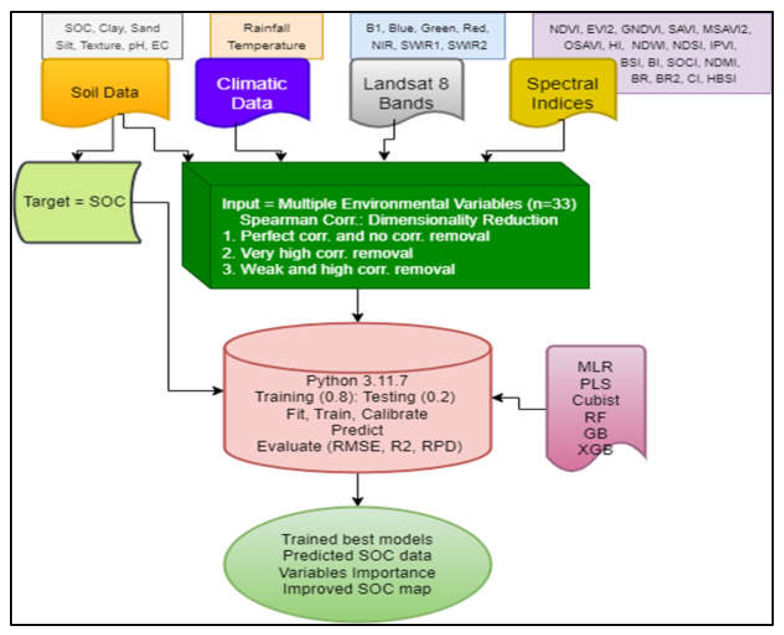
Figure 4.
Observed SOC in the study area.
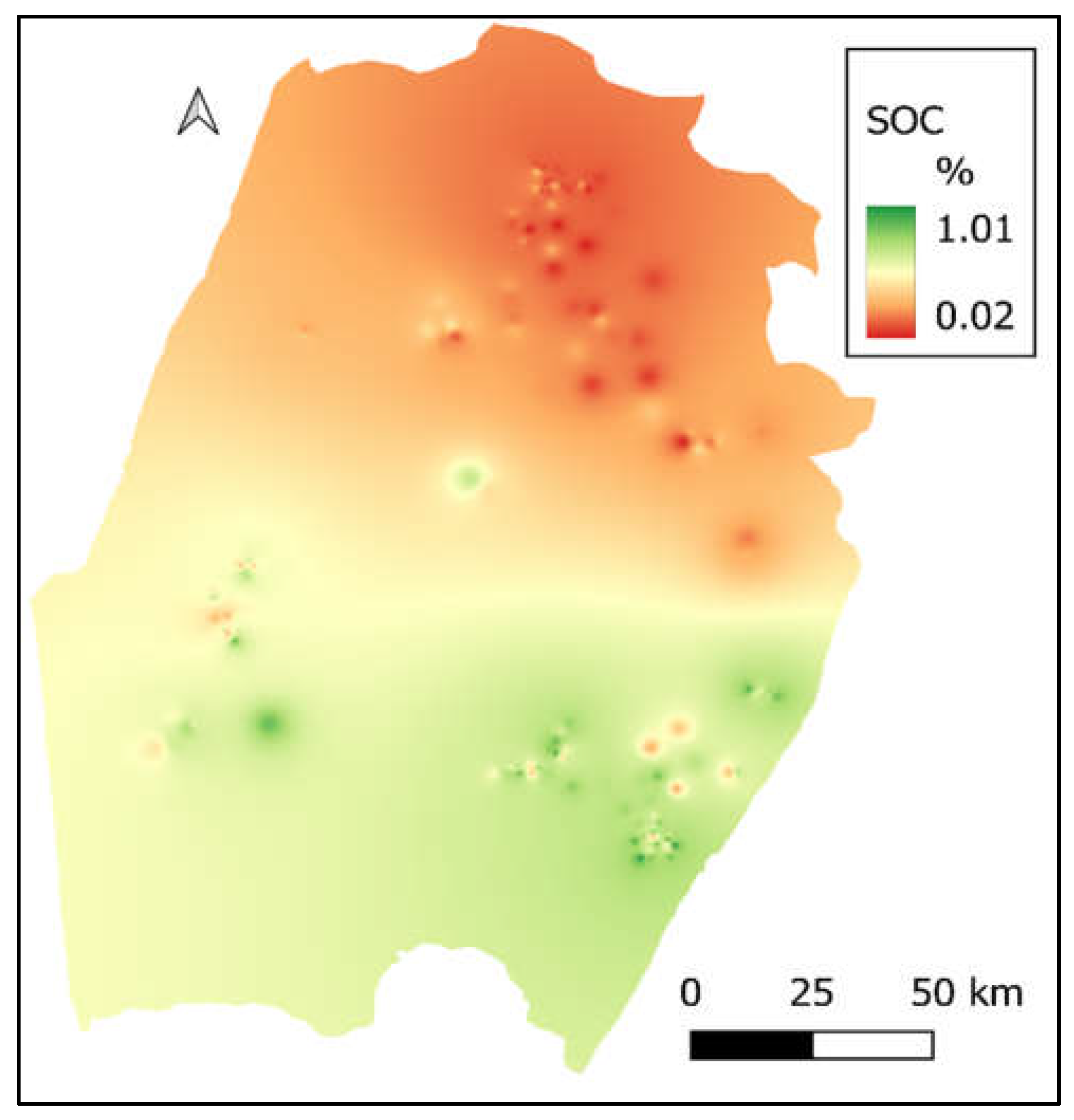
Figure 6.
RF model: variables importance with 25, 14, and 06 input variables, respectively.
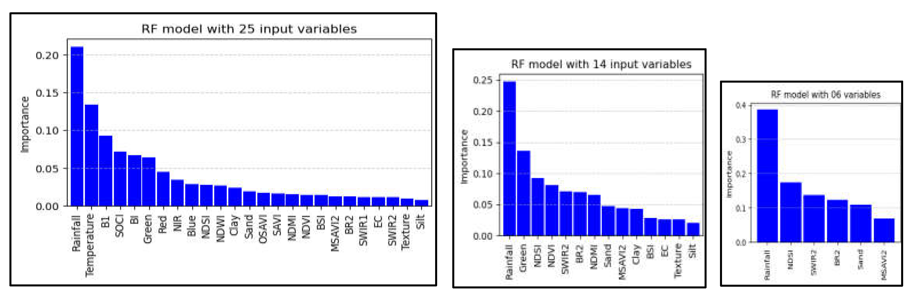
Table 1.
Proposed potential SOC predictor variables, their resolutions and sources.
| Variable Type | Variables | Resolution | Source |
|---|---|---|---|
| Soil | Clay, Silt, Sand, Texture, pH, EC | Lab measurement | |
| Climatic | Temperature, Rainfall | 1 km | WorldClim 2.1 |
| Spectral indices | NDVI, GNDVI, IPVI, EVI2, SAVI, OSAVI, MSAVI2, NDWI, NDSI, BSI, HBSI, SOCI, NDMI, BR, BR2, CI, HI, BI | 30 m | Computed using their formula |
| L8 bands | B1, Blue, Green, Red, NIR, SWIR1, SWIR2 | 30 m | Landsat sensor |
Table 2.
Proposed spectral indices and L8 bands, their formula/wavelength and references.
| Formula/Wavelength | References |
|---|---|
| NDVI = (NIR – Red)/(NIR + Red) | [32] |
| GNDVI = (NIR−Green)/(NIR+Green) | [33,34] |
| EVI2 = 2.5[(NIR – Red)/(NIR + 2.4*Red + 1)] | [35] |
| IPVI = NIR/(NIR + Red) | [29] |
| SAVI = ((NIR – Red)/(NIR + Red + 0.5))*(1+0.5) | [31] |
| OSAVI = (NIR – Red)/(NIR + Red + 0.16 | [36] |
| MSAVI2 = 0.5[2*NIR+1− √ [(2*NIR+1)2 − 8(NIR−Red)]] | [37] |
| NDWI = (Green – NIR)/(Green + NIR) | [29] |
| NDSI = (SWIR1 – Green)/(SWIR1 + Green) | [38] |
| BSI = [(SWIR2 + Red) – (NIR + Blue)]/[(SWIR2 + Red) + (NIR + Blue)] | [39] |
| HBSI = [(SWIR2+Green)−(NIR+Blue)]/[(SWIR2+Green)+(NIR+Blue)] | [34] |
| SOCI = Blue/(Red*Green) | [31,40] |
| NDMI = (NIR-SWIR1)/(NIR+SWIR1) | [41] |
| BR = (NIR-SWIR2)/(NIR+SWIR2) | [42] |
| BR2 = (SWIR1-SWIR2)/(SWIR1+SWIR2) | [43] |
| CI = (Red – Green)/(Red + Green) | [44] |
| HI = (2*Red – Green – Blue)/(Green – Blue) | [44] |
| BI = √ [(Red2 + Green2)/2] | [34,45] |
| Blue 0.450 - 0.510 µm | [27,46] |
| Green 0.530 - 0.590 µm | [27,46] |
| Red 0.640 - 0.670 µm | [27,46] |
| NIR 0.850 - 0.880 µm | [27,46] |
| SWIR1 1.570 - 1.650 µm | [27,46] |
| SWIR2 2.110 - 2.290 µm | [27,46] |
Table 4.
Performance of Models for SOC prediction with different number of input variables.
| No. of Variables | Metrics | PLS | Cubist | XGB | GB | MLR | RF |
|---|---|---|---|---|---|---|---|
| 25 | RMSE | 0.128 | 0.131 | 0.129 | 0.129 | 0.143 | 0.141 |
| R2 | 0.776 | 0.778 | 0.775 | 0.784 | 0.737 | 0.743 | |
| RPD | 2.147*** | 2.097*** | 2.141*** | 2.125*** | 1.925** | 1.949** | |
| 14 | RMSE | 0.113 | 0.122 | 0.126 | 0.135 | 0.135 | 0.141 |
| R2 | 0.827 | 0.808 | 0.783 | 0.764 | 0.764 | 0.745 | |
| RPD | 2.439*** | 2.257*** | 2.177*** | 2.034*** | 2.032*** | 1.956** | |
| 06 | RMSE | 0.131 | 0.141 | 0.124 | 0.142 | 0.133 | 0.144 |
| R2 | 0.767 | 0.713 | 0.792 | 0.739 | 0.758 | 0.703 | |
| RPD | 2.104*** | 1.950*** | 2.224*** | 1.933** | 2.062*** | 1.917** |
** and *** indicate good and very good models, respectively [47] .
Disclaimer/Publisher’s Note: The statements, opinions and data contained in all publications are solely those of the individual author(s) and contributor(s) and not of MDPI and/or the editor(s). MDPI and/or the editor(s) disclaim responsibility for any injury to people or property resulting from any ideas, methods, instructions or products referred to in the content. |
© 2025 by the authors. Licensee MDPI, Basel, Switzerland. This article is an open access article distributed under the terms and conditions of the Creative Commons Attribution (CC BY) license (http://creativecommons.org/licenses/by/4.0/).
Copyright: This open access article is published under a Creative Commons CC BY 4.0 license, which permit the free download, distribution, and reuse, provided that the author and preprint are cited in any reuse.


