
Submitted:
27 October 2025
Posted:
28 October 2025
You are already at the latest version
Abstract
Soil organic carbon (SOC) is a key component of terrestrial ecosystems, serving as an energy source for soil microorganisms and playing an essential role in climate regulation and ecosystem productivity. However, SOC stocks are highly influenced by land-use and land-cover changes. This study aims to estimate and map SOC using multispectral Sentinel-2 and RapidEye imagery combined with environmental, soil, and topographic variables across Khat-dominated landscapes in the Haramaya district, eastern Ethiopia. A total of 88 soil samples were collected and analyzed in the laboratory for organic carbon estimation. Two machine learning algorithms, Random Forest (RF) and Extreme Gradient Boosting (XGB), were applied to predict SOC, and their performances were evaluated using the coefficient of determination (R²), root mean square error (RMSE and mean absolute error (MAE). Laboratory-measured SOC values ranged from 0.83% to 3.9%. Both satellite datasets produced comparable predictions, with Sentinel-2 estimating slightly higher mean SOC values (~40mg/ha), while RapidEye(~38mg/ha) provided more spatially detailed and accurate maps due to its finer resolution. Among the algorithms tested, RF outperformed XGB, showing higher predictive accuracy and stability, particularly under heterogeneous landscape conditions. The results suggest that both Sentinel-2 and RapidEye data are suitable for SOC estimation and mapping, with higher-resolution imagery preferred for detailed spatial analysis. Future research should focus on optimising predictor selection and assessing the potential impacts of Khat cultivation on SOC variability and spatial distribution.
Keywords:
Haramaya District
; SOC
; RapidEye
; Sentinel-2
; LULC
; Khat cultivation
; ML
1. Introduction
Soil organic carbon (SOC) is the essential foundation of healthy soil, supporting diverse microbial life belowground and driving vital processes like nutrient recycling, water retention, and ecosystem resilience [1,2]. Importantly, as the planet’s largest land-based carbon reservoir, SOC functions as a vast underground store, directly affecting atmospheric CO₂ levels and making its careful management as one of our most potent tools for climate change mitigation [3]. Increasing SOC stocks not only creates more fertile, resilient farmland resistant to droughts and floods but also actively removes carbon from the atmosphere, encouraging sustainable agriculture and strengthening global efforts toward a healthier planet [2,4]. Protecting and restoring this crucial resource is key to maintaining resilient landscapes, ensuring long-term food security, and achieving critical climate targets [1].
SOC has been continuously disturbed by land use changes, intensive grazing, and cultivation. As SOC represents one of the major pools in the global C cycle, small changes in SOC stocks cause significant CO2 fluxes between terrestrial ecosystems and the atmosphere [5]. Soil carbon stock varies with land use and management practices, leading to a high level of uncertainty in the data. Worldwide, numerous studies have documented a decline in SOC stocks due to the degradation of natural ecosystems or the conversion of natural areas into intensively cultivated croplands [6,7]. Determining SOC content is a key part of research in assessing fluxes.
In Ethiopia, a rapid agricultural transformation is underway as smallholder farmers increasingly convert their agricultural farms to Khat (Catha edulis) cultivation. This transformation is evident in Haramaya District, where the rapid expansion of Khat cultivation, known as a perennial shrub and dominant cash crop, has significantly altered traditional agricultural landscapes, often replacing food crops and natural vegetation [8,9]. Khat’s cultivation, which provides superior economic returns, primarily drives this shift compared to other perennial or annual crops. The Khat crop’s appeal also stems from its potential for year-round harvesting, and use as a stimulant plant by most local communities, especially in southern and Eastern Ethiopia [8,9]. This shift raises concerns about its impact on SOC dynamics, as Khat farming could potentially alter organic matter inputs, increase soil disturbance, and accelerate erosion, with effects varying by management practices and landscape position [10]. Understanding the spatial distribution and potential of SOC in this intensively managed and rapidly transforming landscape is essential for developing sustainable land management strategies and supporting climate change mitigation efforts.
Despite these significant land-use changes caused by Khat cultivation, a critical knowledge gap remains regarding the soil organic carbon content across Khat-cultivated farms. Therefore, understanding how different land uses influence SOC stock potential is vital, as this offers profound insights into SOC dynamics than merely studying total SOC alone [4,11,12,13,14]. Furthermore, accurate estimation of SOC storage is essential for evaluating both carbon sequestration capacity and emissions from land-use changes. Nevertheless, the high spatial variability of SOC stocks across different land-use types and management practices introduces considerable uncertainty in estimating SOC at regional and global levels. Above all, traditional methods for assessing SOC lack the spatial resolution and scalability needed to capture the complex interactions among vegetation, soil, and land management, underscoring the need for advanced mapping tools to support informed decision-making [15]. Therefore, a dependable assessment of these carbon pools is necessary for informed decision-making.
Traditional methods for assessing SOC, such as field sampling and laboratory analysis, are labour-intensive, time-consuming, and have limitations in measuring carbon on a large scale, making it challenging to capture a detailed spatial heterogeneity of SOC across diverse and dynamic landscapes like the Haramaya District [16,17]. In contrast, remote sensing technologies offer a cost-effective and scalable alternative by providing spatially continuous data at various temporal and spatial resolutions [18,19]. The high-resolution nature of these images provides detailed insights into soil heterogeneity patterns, while being significantly more cost-effective than traditional methods [16,20,21,22,23,24,25,26]. Satellite-derived vegetation indices, including the Normalized Difference Vegetation Index (NDVI), Soil Adjusted Vegetation Index (SAVI), and Bare Soil Index (BSI), have been shown to correlate well with SOC content, as they reflect key indicators such as vegetation cover, biomass levels, and soil exposure [27,28]. Previous research has confirmed the effectiveness of these indices for digital SOC spatial modelling [17,29,30,31,32].
In this study, where smallholder Khat cultivation is rapidly expanding, satellite imagery from platforms such as Sentinel-2 and RapidEye can be utilized to derive these indices and monitor land cover changes associated with various land management practices. These satellites can capture data across multiple spectral ranges, including the visible, infrared, near-infrared, and short-wave infrared regions. This capability allows for the computation of various vegetation indices that correlate with SOC content, which is valuable for estimating SOC across heterogeneous landscapes. Similarly, combining remotely sensed data with ground-based SOC measurements can facilitate the development of robust machine learning models aimed at improving the accuracy and efficiency of SOC mapping and monitoring over large areas [33,34]. Applying machine learning and remote sensing for SOC mapping supports evidence-based decision-making for sustainable land management. These techniques enable the ongoing monitoring of SOC in response to changes in land use.
Machine learning (ML) techniques have transformed digital soil mapping by enabling accurate prediction of SOC through modelling complex, non-linear relationships with environmental variables [35]. This computational advance, coupled with the increasing availability of high-resolution satellite data, has opened up new opportunities for efficient, scalable, and precise SOC estimation [36]. ML algorithms such as Random Forest (RF), Support Vector Machines (SVM), deep learning models, XGBoost, and Gradient Boosting models have shown superior performance in predicting SOC over traditional statistical methods [15,34,37]. ML models can manage high-dimensional data and capture intricate interactions among predictors, including remote sensing indices, topographic variables, and soil properties, to produce high-resolution maps of soil carbon potential. In regions like Haramaya District, where Khat cultivation dominates the landscape, generating such maps is vital for identifying zones with high SOC potential. Combining remote sensing and machine learning improves prediction accuracy and provides deeper insights into the key environmental and land management factors affecting SOC variability in rapidly changing agricultural landscapes. This integrated approach is especially valuable for supporting sustainable land use planning, climate mitigation strategies, and evidence-based policymaking in regions experiencing rapid agricultural transformation.
SOC shows notable spatial variation due to environmental and human factors; however, most current research has focused on regional to global scales, limiting its ability to capture detailed local differences essential for land management and climate change initiatives. Therefore, this study employs a machine-learning framework in Ethiopia’s Haramaya District, combining Sentinel-2 and RapidEye satellite-derived vegetation indices with topographic, climatic, and field data to estimate SOC stocks across diverse landscapes. The goals are to: (1) measure SOC content across various land-use types, (2) evaluate how accurately satellite imagery predicts SOC, and (3) create high-resolution maps of SOC distribution in the Khat-dominated landscape. This integrated approach provides an affordable means of assessing SOC, enhances understanding of spatial variability and its environmental drivers, and underscores the utility of remote sensing for carbon monitoring. The findings provide solid, data-driven insights to support sustainable land management and climate strategies, especially for local practitioners and policymakers in Ethiopia.
2. Materials and Methods
2.1. Study Area Description
The Haramaya District is in the eastern part of the Hararghe Zone within the Oromia Region of Ethiopia, approximately 506 kilometers east of Addis Ababa. The district’s geographic coordinates range from 41°54’0’’ to 42°4’0’’ east longitude and from 9°8’15’’ to 9°29’15’’ north latitude (Figure 1). The area occupies a strategically significant position near several administrative boundaries.
The district features a semi-arid tropical belt and experiences bimodal rainfall (600–1260 mm annually) during the Badheessa (March-May) and Ganna (June-September) seasons. Its climate is composed of 66.5% midland and 33.5% lowland, with temperatures ranging from 6-12°C minimum to 17-25°c °C maximum [38]. Although the district lacks perennial rivers, it has the seasonal Hamaresa stream and a dendritic drainage pattern. Recent developments since 2019 include the restoration of Lake Haramaya and the expansion of Lake Adele.
A 1995/96 land use survey of Haramaya District showed that 36.1% of the total area was arable land, 2.3% pasture, and 1.5% shrubland (forest). The remaining 60.1% consisted of degraded or built-up areas (Figure 1). Steep slopes and heavily degraded zones are characterized by shrub and bush cover, rock outcrops, and vegetation dominated by invasive species such as Lantana camara, cactus, and stunted Acacia abyssinica. Remnant forests, including species like Juniperus procera, Podocarpus nubigenus, and Olea europaea, remain on slopes and field margins. However, widespread degradation is closely linked to the expansion of Khat (Catha edulis) cultivation.
The dominant farming system involves mixed cropping, primarily involving sorghum and maize intercropped with khat, beans, and sweet potatoes, alongside livestock husbandry [38]. The middle to lower slopes is under intensive cultivation. Common soil types include Luvisols, Cambisols, Vertisols, and Nitisols. Overall, the landscape reveals significant ecological disturbance resulting from agricultural pressure and the economic importance of Khat cultivation. This has resulted in reduced natural vegetation cover and exacerbated land degradation.
2.2. Field Sampling Procedure and Laboratory Analyses
The SOC data was gathered through direct field surveys using a stratified random sampling approach. This process involves initial plot mapping using topographic maps and satellite images, dividing the study area into layers based on land use and land cover type. Representative soil samples are then collected from sample points within each layer. Systematically spaced 20-meter plots were established throughout the layers, with GPS used to record the centroid coordinates of each plot. In each plot, five soil subsamples were collected from the 0–20 cm depth using a soil auger, following a systematic quadrant method (one at each corner and one at the centre). These subsamples are then combined into a composite sample weighing about 0.5 kg to minimize spatial variability, following standard quadrant procedures. At the same time, undisturbed soil cores for bulk density analysis were taken from the plot centre using a volumetric core sampler to reduce soil disturbance. The 0–20 cm depth was chosen because of its importance in agroecological processes, including soil organic matter dynamics, root biomass distribution, and key human activities such as tillage and nutrient cycling [39]. Ultimately, 88 composite samples were processed under controlled conditions, with chain-of-custody procedures maintained during transportation to Haramaya University Soil Laboratory for physicochemical analysis. This approach enhances the representativeness of surface soil properties and aligns with established pedometric frameworks for agronomic and soil research.
Sample preparation involved two distinct processes:
- For soil organic carbon analysis: Disturbed samples were air-dried, crushed, and passed through a 0.5 mm sieve
- For bulk density determination: Undisturbed samples were oven-dried at 105°C to determine soil bulk density using the following equation (Eq. 1):
The soil organic carbon content was analysed by the wet digestion method as described in [40], a standard procedure in Ethiopia that involves digesting the organic carbon in soil samples with potassium dichromate (K2Cr2O7) in a sulfuric acid solution. Following this procedure, the soil carbon content (%) was estimated for each land cover type or stratum. The calculation for the SOC stock, as described in [41] is as follows:
SOCi stock (Mg C Ha-1 = OCi * BDfine2i * ti * 0.1
Where,
- SOCi (Mg C ha-1) is the organic carbon stock of depth increment i; OCi (mg C g-1 fi ne earth) is the organic carbon content of the fine earth fraction (< 2 mm) in the depth increment i;
- BD fne2i (g fine earth cm-3 soil) is the mass of ne earth per total volume of the soil sample = mass (g) of fine earth / total volume of soil sample (cm3 ) in the depth increment i;
- ti is the thickness (depth, in cm) of the depth increment i;
- is a factor for converting mg C cm-2 to Mg C ha-1
This equation is a simpler calculation for which fewer measurements are needed and less uncertainty is involved, as there is no need to determine or assume the volume of the coarse fraction
2.3. Remote Sensing Image Acquisition and Processing
The study combined field data and spectral information to evaluate SOC across different land use types. Multispectral satellite images from Sentinel-2 (https://dataspace.copernicus.eu/) and RapidEye from Planet Explorer (www.planet.com/explorer) were acquired from the mentioned website. These satellites are geometrically and radiometrically corrected to improve the analysis of surface features at various scales. Sentinel-2 consists of two polar-orbiting satellites with 13 spectral bands ranging from 10 to 60 m in the VNIR to SWIR wavelengths. It is regarded as high spatial resolution satellite data, providing valuable information for monitoring soil carbon fluxes and other land characteristics [37]. The RapidEye satellite image, on the other hand, is among the very high-resolution (VHR) imagery with five bands (blue, green, red, red-edge, and near-infrared) of 5m spatial resolution, making it suitable for more accurate environmental studies [42]. The following key remote sensing indices, including MSAVI, GNDVI, BSI, NDMI, SAVI, NDWI, TVI, were derived from the selected satellite imagery together with other environmental variables used as input for SOC modelling. Table 1 shows the spectral indices and their commonly used formulas for calculation from Sentinel 2- and RapidEye data.
The satellite imagery acquisition spans from February to April 2019, a period chosen to align with field data collection. The raw data underwent several pre-processing steps, including mosaicking, layer stacking, and data subset selection. The land use/land cover classification was performed using the Google Earth Engine (GEE) Claude platform by employing a supervised classification technique.
2.4. Terrain, Soil and Climatic Variables.
Terrain variables were extracted from the 30 m resolution ASTER GDEM [49]. This dataset is freely available. The data was pre-processed to create a depressionless DEM before calculating terrain variables. The pre-processed DEM was used to derive Slope, Elevation, and Topographic Wetness Index. Climatic data (e.g., mean monthly rainfall and land surface temperature) were obtained from CHRIPS and MODIS datasets. Additionally, soil information, such as clay, bulk density, cation exchange capacity (CEC), and sand content, as well as plant biophysical properties, including Fraction of Absorbed Photosynthetically Active Radiation (fAPAR) data, were sourced from ISRIC and MODIS datasets.
Overall, a total of seventeen (17) remote sensing, topographic, and environmental variables were used to train the model and predict SOC. To ensure integration with RapidEye and Sentinel-2 data, all topographic, soil, and climatic variables were resampled to 5- and 10-m resolutions using bilinear interpolation methods, respectively. Table 2 lists the input variables used in this study. Data processing and transformation were performed using ArcGIS Pro and R software.
2.5. ML Approaches and Description of the Models
Integrating remote sensing data with machine learning has proven cost-effective and offers a better opportunity for SOC estimation. In this study, we employed two ML models for SOC prediction, which are recommended by different researchers, such as eXtreme Gradient Boosting (XGBoost) [50], and RF [37,51]. These selected ML techniques are well-suited for handling multidimensional datasets and effectively addressing the collinearity challenges commonly encountered in environmental data for accurately predicting soil parameters [37,51,52]. Moreover, they have been extensively used and are reliable approaches for SOC prediction and retrieval studies, demonstrating solid predictive performance and robust simulation results. Importantly, they are computationally simple.
Random forest is a classifier or regression model that consists of many classification and regression trees, each of which depends on the values of a random vector sampled independently and with the same distribution for all trees in the ensemble data [53]. The RF model is assumed to be robust with respect to handling collinearity among predictors and noisy covariates [54]. It contains not a single standard regression tree but many regression trees, like a forest. RF improves prediction accuracy and reduces model complexity overfitting [55]. It is insensitive to missing data and can handle extensive quantities of quantitative and categorical data [56] . Unlike other models, RF only requires two parameters to be set for generating a prediction model: (i) the number of regression trees to grow in the forest, and (ii) the number of randomly selected evidential features at each node. By default, the random subset size is the square root of the total number of predictors in the model. Furthermore, the RF model demonstrated improved capability in predicting SOC across different land-use types [37].
The XGBoost algorithm is a powerful tree-based approach that has recently attracted considerable interest in digital soil mapping [57]. Gradient boosting builds additive regression models by sequentially fitting a simple, parameterized function (base learner) to the current “pseudo”-residuals using least squares at each iteration [58]. XGBoost is renowned for its robustness and high predictive accuracy, particularly in handling complex nonlinear relationships between variables. For example, it has been successfully used to map soil nutrients and various other soil properties[59,60]. The learning process in XGBoost is incremental: the first learner models the input data space, and subsequent models are trained to correct the errors of the previous learners. This correction process is repeated multiple times until the error criterion is minimized. XGBoost has been widely used in many applications, including SOC estimation, and often delivers superior results compared to standard classification approaches [57,58].
2.6. Model Development and Evaluation
The selected ML methods are well-known for their general predictive abilities and are commonly used for estimating and predicting soil properties, especially SOC. This study employs the R programming language within R-Studio for modelling and data analysis. The collected dataset was split into training (70%) sets and a validation/testing set (30%), using a standard machine learning approach. A 10-fold cross-validation method with three replications was applied to assess the model prediction performance [61]. This approach enables the creation of train/test splits within the dataset, providing an opportunity for each data point to be included in the test set at least once, thereby reducing bias in smaller datasets. Additionally, various model regularization methods were applied to tune the model and improve accuracy. By running the models 10 times, we obtained 10 results to calculate the ensemble mean and standard deviation for SOC estimation.
A statistical model was assessed using predicted SOC and the field-measured SOC for each selected ML model. To determine the best-performing models for SOC estimation, a range of evaluation statistics, such as the coefficient of determination (R2), root mean square error (RMSE), and the mean absolute error (MAE), were used. Ultimately, the model with the highest R2 and the lowest MAE and RMSE was selected to generate the spatially distributed SOC mapping for the study area [62]. Furthermore, to understand the most essential variables in the model, a variable importance factor (VIP) was computed.
The formula used to compute the accuracy metrics using the predicted and measured SOC are shown below [37,63,64]
Finally, the best model was used to derive a SOC variability map for the region using ArcGIS Pro.
3. Results
3.1. Land Use Land Cover (LULC) Analysis
LULC in the Haramaya District was classified from 2020 Sentinel-2 imagery using Google Earth Engine (Figure 11). Six broad LULC classes were identified, namely: bare-grass-shrub, agriculture, natural vegetation, built-up areas, Khat cultivation, and water bodies. Of the total area (56,471 ha), vegetation accounted for the most significant proportion, at 15,510 ha (27.47%), followed by agriculture at 15,142 ha (26.81%) and Khat cultivation at 15,069 ha (26.68%). Bare/grass-covered 8,005 ha (14.18%), while built-up areas occupied 2,273 ha (4.03%). Water bodies represented the smallest class, covering only 472 ha (0.84%) (Table 3). This indicates that vegetation, agriculture, and Khat cultivation are the primary land cover types in the district, while water bodies comprise the smallest land use class.
The overall classification accuracy for the LULC map created using supervised methods was 82.5%, with a kappa coefficient of 0.75%.
3.2. Soil Bulk Density and Organic Carbon
Table 4 presents the laboratory-measured organic carbon (OC) content and bulk density of the soil samples. The results indicate that the average OC is about 1.39%, and the mean bulk density is 1.36 g/cm³. These values indicate that the soils have moderate organic carbon levels, and the measured bulk density suggests relatively compact soil conditions, which could impact soil fertility, water retention, and carbon storage capacity.
3.3. Correlation Between Remote Sensing-Derived and Environmental Variables with SOC
The correlation analysis indicates that SOC generally exhibits weak relationships with individual predictors, reflecting its dependence on complex interactions among environmental, topographic, and spectral factors (Figure 2a & b). Among these, GNDVI (r = 0.20) and BSI (r = 0.12) derived from RapidEye imagery, rainfall (r = 0.20), CEC (r = 0.12), clay content (r = 0.13), and LULC (r = 0.13) show consistently positive correlations, highlighting their contributions to SOC distribution. In contrast, most other variables display negative or very weak correlations with SOC, indicating limited direct influence. Notably, TWI exhibits a slightly stronger negative relationship, suggesting a modest contribution of topographic factors to SOC variability. Overall, these findings emphasize that accurate SOC prediction relies on the integration of topographic, soil, and spectral predictors, with RapidEye imagery demonstrating comparatively greater potential than Sentinel-2 in capturing spatial SOC patterns across the study area.
3.4. RapidEye and Sentinel-2-Based SOC Prediction
The RF-based model performance comparison highlights clear trends with the two satellite data sets for SOC predictions (Figure 3). Sentinel-2 data shows a reasonable correlation between actual and predicted SOC, with moderate prediction accuracy. The scatterplot suggests variability; some points closely align with the regression line, while others exhibit noticeable deviation. Sentinel-2’s spectral resolution, particularly in the red-edge and shortwave infrared bands, enhances SOC sensitivity but may not fully capture spatial variability at finer scales. The model explains approximately 30.4% of the variation in measured SOC, with an RMSE of 7.3% and an MAE of 5.7%.
The performance of RapidEye data was slightly better (R² = 0.33, RMSE = 7.1%, and MAE = 5.8%). This suggests that RapidEye’s higher spatial resolution (5 m compared to Sentinel-2’s 10 m) better captures the local heterogeneity influencing SOC estimation. However, the improvement is not significant, indicating that both sensors yield comparable SOC estimates from the RF models. However, Sentinel-2 remains a strong alternative due to its free access and broader coverage.
In contrast, the XGBoost (XGB) model produced higher errors (RMSE/MAE) and lower R² values, showing greater sensitivity to input data characteristics. The model performed poorly for both datasets (R² = 0.11 for RapidEye and 0.15 for Sentinel-2). Overall, RF demonstrated better consistency and lower prediction bias than XGB across both data types, consistently producing lower RMSE/MAE values (7.19 vs. 8.16 for RapidEye; 7.34 vs. 9.26 for Sentinel-2). The results from the RF model were used in further analysis. Overall, considering the R2 value our finding shows relatively lower R2 value for SOC estimate, which can be linked to the incorporation of the larger number of predictors may introduce additional variability or noise, thereby reducing model precision (Appendix)
3.5. Variable Importance Ranking for SOC
The challenges in SOC modelling lie in identifying the factors responsible for SOC changes. In this study, we presented the most essential covariates identified by the RF model in both datasets, indicating which data are most helpful for SOC prediction in the study area. The VIP for the RapidEye dataset shows that the most critical predictors for SOC are a balanced combination of spectral indices and topographical/soil properties, confirming the model’s reliance on multiple data sources (Figure 4). The GNDVI remains the most significant predictor, measuring vegetation greenness. Since SOC is highly correlated with areas characterised by high vegetation (greenness), GNDVI measures the direct spectral absorption of organic matter in the visible spectrum. Abbaszad et al[65] also found GNDVI as the most critical remote sensing index for SOC prediction, which agrees with our findings. Soil-related indices, such as SAVI[35], are identified as the second-most important remote sensing indices for SOC estimation. Other remote sensing indices, such as the Transformed Vegetation Index (TVI), fAPAR, and BSI, are ranked as moderately important for SOC estimation. They serve as a surrogate for current or historical biomass productivity, providing a spatial layer that correlates with the source of organic carbon. Moisture index, such as NDMI, is listed among the least contributing remote sensing indices for SOC in the study area.
The environmental and physical parameters align with the spectral indices, indicating that a predictive model for SOC requires more than remote sensing data alone. These variables provide the non-spectral context for carbon stability. A higher ranking for the Topographic Wetness Index suggests that it acts as a proxy for broad environmental gradients, including microclimate (temperature, moisture) and general geological/soil formation processes across the landscape [66,67]. From the soil parameters, Clay content and CEC are ranked as the most important variables, which is critical because clay minerals physically bind and protect organic carbon from decomposition, making them powerful predictors of the soil’s long-term carbon storage capacity, independent of current spectral conditions [68,69,70]. LST is also listed as an essential contributor, which can influence the biological decomposition rates of organic matter.
3.6. SOC Computed per Land Use Class/Types from the RapidEye and Sentinel-2 Data
The results indicate variation in SOC content across different land use and land cover types as estimated from RapidEye and Sentinel-2 data (Table 5). Among the LULC classes, forest areas exhibited the highest mean SOC values (38.9 mg/ha from RapidEye and 40.4 mg/ha from Sentinel-2), reflecting the positive influence of dense vegetation and organic matter accumulation. The agricultural and Khat-cultivated lands showed relatively similar mean SOC value estimates (around 38.6–38.7 mg/ha from RapidEye and 40.5–40.6 mg/ha from Sentinel-2), suggesting moderate SOC retention likely due to regular cultivation and organic residue input. Similarly, the bare-grass-shrub areas had comparable mean SOC values (38.7 mg/ha from RapidEye and 40.7 mg/ha from Sentinel-2). However, the range was broadest under Sentinel-2 (8.2 mg/ha), indicating greater spatial variability within this class. The generally slightly higher means and wider ranges in Sentinel-2 data may be attributed to its broader spectral coverage and improved sensitivity to surface conditions. This enables better detection of SOC variability across land cover types compared to RapidEye imagery, which is highly influenced by soil background due to its high resolution. Importantly, because the 10 m land-use (LU) map was derived from Sentinel-2 imagery, SOC estimates across LU classes were more consistent and direct than those derived from RapidEye data. Subsequently, resampling the same LU layer to a 5 m resolution could have increased heterogeneity within the LU classes, leading to slightly lower SOC estimates for those classes.
3.7. Spatial Variability Mapping of the SOC from RapidEye and Sentinel-2 Data
The spatial distribution map of SOC, derived from the best-performing models using RapidEye and Sentinel-2 datasets, is shown in Figure 5. RapidEye-based spatial maps revealed finer spatial variation, with SOC values ranging from 32 to 41 Mg/ha, compared to 34–44 Mg/ha for Sentinel-2. Although the ML model in Sentinel-2 achieved slightly higher overall predictive performance, RapidEye imagery, which is considered higher resolution, still provided more precise spatial SOC estimates, demonstrating its ability to capture local heterogeneity in soil organic potential mapping. Higher SOC concentrations were observed in the northern and middle (central) parts of the district, primarily associated with Khat cultivation, forest and mixed agricultural land use. Conversely, areas covered by water bodies, bare land, and urban settlements registered lower SOC stocks (Figure 5).

4. Discussion
The LULC analysis shows that Haramaya District is predominantly covered by shrub-vegetation, agriculture, and Khat cultivation (~81%). This has also been reported by Gebere, Alamirew [71]. In the district, due to over-extraction of water for small-scale khat cultivation and an increase in built-up land area, there was a significant decline in groundwater levels and a reduction in surface water [71]. The increasing distribution of mixed land-use practices indicates that subsistence farming and cash crop production (particularly Khat crops) play key roles in the local economy[72]. This could facilitate the trend of expanding Khat cultivation areas further beyond the current extent [8,72,73]. This intern could affect the SOC stock. Importantly, this LULC composition has direct implications for SOC distribution, as areas dominated by vegetation, agriculture, and Khat cultivation are expected to have significantly varying SOC stocks compared to bare/grass, built-up, or water-covered areas. Although there is not much difference in SOC variation among LU types observed at the time of the study, there is a high likelihood that the trend will change, particularly if a large portion of the forest area is converted to mixed cultivation or a significant portion is used for Khat cultivation. The other reason for the lack of substantial difference among SOC estimates between LU could be attributed to the fact that the majority of the area remaining under Khat cultivation throughout the year(the dominant land use ), leading to the denudation of biomass, which could contribute to SOC accumulation [10,74].
The average OC distribution estimate in the current study is 1.39%, with a minimum of 0.83% and a maximum of 3.9%,which was found consistent with those of Mohammed, Kibebew [75], who estimated low soil OM content of 1.02 to 3.92% in the subcatchment (around Lake Haramaya) of the district. The dominance of agricultural and Khat-cultivated areas across the district may be a reason for the low OC content, due to the practice of completely removing crop residue and the minimal application of farmyard manure [9,10,74]. In the district, crop residue is often entirely removed for livestock feed and household fuel, a standard practice that leads to low SOC content [76]. The other possible reason for the low SOC content in the district is that the majority of khat and agricultural land is irrigated, leading to less organic matter being oxidised than eroded by cultivation and other processes. For instance, Negash, Kaseva [74] found higher SOC loss (three times greater) in areas dominated by single khat crops than in mixed agroforestry systems (khat and Coffea arabica), which could also be the case in our study area. According to this report, the mean annual rate of SOC decline after native forest conversion to khat was estimated at 4.89 Mg/ha, higher than for other land-use types. Likewise, Mellisse, Tolera [10] reported a significant reduction in total biomass carbon/organic matter in khat-dominated land-use areas within the Wondo Genet landscape of southern Ethiopia.
The comparison of SOC estimates using Sentinel-2 and RapidEye imagery shows consistent spatial patterns but resolution-dependent differences in magnitude and variability. Sentinel-2 produced slightly higher average SOC values (~40 Mg C ha-1) with low variability; conversely, RapidEye yielded slightly lower average SOC values (38 Mg C ha-1) with a narrower range between the minimum and maximum SOC estimates. The SOC content reported in the current study is in agreement with that of [13,77] who reported 33 to 38 Mg C ha−1 of SOC at the Gum Selassa site in Northern Ethiopia, and 33.2-34.7 Mg C ha-1 in the Azuga suba and Yesir selected watersheds of Ethiopia, using MODIS and legacy data based on the RF model. However, the SOC estimated mean in this study is slightly higher than the reported SOC by [67] (21-37 g/kg) for different sites in the Blue Nile basin. Nevertheless, the SOC estimate is much lower than the SOC content estimated for the Khat cultivated area and mixed agroforestry practice landscape in southeastern Ethiopia [74]. Similarly, the SOC estimated from both datasets in this study is much lower than the SOC estimated by [78], using the Landsat8 OLI dataset in the Dominican Republic forest landscape. The min-max range of SOC estimations for different landuse types using RapdEye was marginally low, which can be attributed to the fact that the estimation was done using 5m resampled landuse data, which was actually derived from 10m Sentinel2 data. Over-sampling would have led to some misclassification, particularly near the class boundaries. Nevertheless, the difference in range is not found to be significant, and with nearly identical mean values, the SOC estimates were found to be consistent with the two datasets and either can be used for SOC estimation for different land use in the study area. However, the spatial distribution of the SOC map from RapidEye showed finer spatial variabilities (Figure 5), demonstrating its ability to capture local heterogeneity in soil organic potential mapping. Higher SOC concentrations were observed in the northern and middle (central) parts of the district, primarily associated with Khat cultivation, forest and mixed agricultural land use. Conversely, areas covered by water bodies, bare land, and urban settlements registered lower SOC stocks. Sentinel-2 tended to overestimate SOC, but it predicted more accurately in water bodies and settlement areas, as shown in Figure 5 (right).
The range of SOC estimates from the two sensors shows that RapidEye predicts a narrower range of SOC values than Sentinel-2, highlighting the benefits of higher-resolution data. These findings suggest that the RapidEye dataset tends to be superior to the Sentinel-2 dataset for detecting localised landscape heterogeneity and for spatial SOC mapping. For detailed SOC mapping and prediction, the combined use of RF model with indices derived from high and moderate-resolution multispectral remote sensing was shown to be potentially helpful for capturing the SOC variability ([79,80].
In this study, 17 key predictors were retained and used as input for the final model development. Remote sensing variables were found to be the most important predictor of SOC estimation, which is consistent with previous findings [69]. Despite differences in spectral indices between sensors, this study identified that environmental and topographic variables consistently dominated SOC prediction, highlighting their central role in determining SOC distribution within the district. These findings emphasized that effective SOC modelling requires integration of spectral indices with terrain and climate variables, as topography and selected soil factors provide strong explanatory power. Incorporating topographic features alongside spectral indices could also enhance model prediction accuracy and lead to improved soil estimation [81]. As SOC varies considerably across space and seasons, Jo, Panja [35] recommended combining spectral (vegetation indices) information and topographic variables for improved SOC estimation rather than relying on a single type of predictor. Consistent with our results, Hengl, Heuvelink [61] identified topographic factors such as elevation and slope as key determinants of SOC content. These factors play a role in SOC accumulation and transportation from one place to another. Likewise, other studies have also noted that topographic and remote sensing indices are major predictors for SOC [79]. The influence of topographic factors on predicting SOC, for example, can be related to corresponding variations in soil temperature, as well as the intensity of cultivation, which is usually higher in lower areas than in higher regions [59].
SOC dynamics are shaped by complex interactions among soil properties, vegetation indices, climate, and topography, necessitating the development of robust predictive models. In addition, the high intrinsic spatial variability of soil properties, the heterogeneous nature of the landscape, and highly variable management practices by farmers are considered as potential sources of noise that can affect model performance in SOC prediction. In this regard, MLs such as RF model provide valuable tools for managing such complexity; however, their performance often varies depending on the dataset characteristics and the area. Our findings are consistent with those of Dahhani, Raji [81,82], who also reported higher SOC prediction performance with the RF model than with XGB using Sentinel-2 data. This can be attributed to the fact that RF, an ensemble of decision trees, flexibly captures nonlinear relationships between SOC and its predictors and is less sensitive to noise or correlated predictors [35]. Nonetheless, among the ML models used for SOC prediction and mapping from remote sensing data combined with that of environmental and topographic related variables, the RF model typically outperformed SVM, XGB, ANN, and GLM model[68,79,80,83]. This shows the RF model is highly suitable for SOC estimation under varying climatic and land use conditions.
In contrast, XGB, which generally requires larger datasets to learn sequential residual corrections effectively, may sometimes overfit when applied to small or sparse datasets, as is the case in this study. Results from RapidEye and Sentinel-2 imagery indicate that RF performed relatively better, explaining SOC variability with moderate errors. In contrast, XGB showed weaker predictive capability and higher error rates under the test dataset. Moreover, XGB requires careful tuning of parameters such as the learning rate, tree depth, regularisation terms, and subsampling rates, which can easily lead to underfitting or overfitting. Our results demonstrated better performance in terms of RMSE and MAE than those reported by [13]. Meanwhile, the estimated R2 values were in agreement with [13], who reported R2 values ranging from 25 to 34 % for highly managed landscapes. However, our R2 based on the training dataset was found to be much higher than that reported by [13] in a selected watershed of highland Ethiopia, indicating that the model performed better on the training data than on the test data. This result may suggest overfitting or that the random data split could have favoured the training set over the test set. Overall, RF proved more reliable at capturing SOC variability across both datasets, highlighting dataset-specific strengths in SOC prediction and mapping. Pouladi, Gholizadeh [79] also suggested that using an adaptive hybrid algorithm and the fusion of multiple data sources could further enhance SOC prediction accuracy in a heterogeneous landscape like Haramaya District.
5. Conclusions
This study used multispectral remote sensing data from Sentinel-2 and RapidEye satellites, combined with machine learning algorithms such as RF, and XGB, to estimate SOC content. Various remote sensing spectral indices, along with environmental, soil, and topographic variables from multiple sources, served as inputs for the SOC prediction models. The results show that Sentinel-2 imagery yielded a slightly higher maximum SOC value and a wider range of SOC estimates than RapidEye imagery. However, the average SOC estimates from both sensors were similar, at around 38 Mg C ha-1 and 40 Mg C ha-1 for RapidEye and Sentinel, respectively. This indicates that both Sentinel-2 and RapidEye data are comparably suitable for mapping SOC stocks across diverse landscapes, such as the Haramaya district, where Khat is a prominent crop. Nevertheless, the digital SOC maps suggest that the RapidEye dataset provides more detailed information on SOC distribution patterns (spatial clusters) than the Sentinel-2 dataset. Among the machine learning models, RF performed better and is more suitable for generating spatial SOC maps, while XGB underperformed. Land use and land cover analysis further revealed that the study area is mainly dominated by agricultural land, primarily characterised by a mix of khat cultivation and bare–grass–shrub land, both of which significantly influence SOC spatial variability in the study area. Overall, this research highlights the potential of multispectral remote sensing data (freely available and commercial) for spatial SOC mapping in complex and heterogeneous landscapes.
Author Contributions
Conceptualization, E.C. ; methodology, E.C and P.S..; software, E.C. and P.S.; validation, E.C., S.F. and M.Y.; formal analysis, E.C. and P.S.; investigation, E.C. and F.B.; resources, E.G.; data curation, E.C., S.F. and P.S.; writing—original draft preparation, E.C. and P.S.; writing—review and editing, P.S., S.F. and E.G.; visualization, E.C. and M.Y.; supervision, P.S.; project administration, E.C.; funding acquisition, E.C. All authors have read and agreed to the published version of the manuscript.
Data Availability Statement
data can be made available on request.
Acknowledgments
The authors would like to acknowledge the support provided by Haramaya University, Office of the Research and Community Services, Vice President. This research was awarded a research grant under Theme 1. Productivity and Environmental Sustainability for Food Security and Poverty Alleviation (Sub-theme-3 - Environment, Natural Resources, and Climate Change) and project code: HURG-2018-01-03_12. We would also like to pass on our appreciation to all stakeholders for their continuous assistance and effort made during the field data collection (Haramaya Districts, Agricultural and Natural Resources Office) and experts from Haramaya University Soil Laboratory (especially Mr. Dheresa, Mr. Yonas, and Mr. Mekonnen). Finally, our appreciation goes to the finance department office, the research cluster of Haramaya University, and the logistics department for delivering on-time services during the project period.
Conflicts of Interest
The authors declare no conflicts of interest.
References
References
- Minasny, B. , et al., Soil carbon 4 per mille. Geoderma, 2017. 292: p. 59-86. [CrossRef]
- Lal, R. , Soil carbon sequestration impacts on global climate change and food security. science, 2004. 304(5677): p. 1623-1627. [CrossRef]
- Sparks, D.L. , Environmental soil chemistry: An overview. Environmental soil chemistry, 1995: p. 1-22.
- Smith, P. , Land use change and soil organic carbon dynamics. Nutrient Cycling in Agroecosystems, 2008. 81(2): p. 169-178. [CrossRef]
- Stevens, A. , et al., Detection of carbon stock change in agricultural soils using spectroscopic techniques. Soil Science Society of America Journal, 2006. 70(3): p. 844-850. [CrossRef]
- Berhongaray, G. , et al., Land use effects on soil carbon in the Argentine Pampas. Geoderma, 2013. 192: p. 97-110. [CrossRef]
- Ashagrie, Y. , et al., Soil aggregation, and total and particulate organic matter following conversion of native forests to continuous cultivation in Ethiopia. Soil and Tillage Research, 2007. 94(1): p. 101-108. [CrossRef]
- Tofu, D.A. and K. Wolka, Climate change induced a progressive shift of livelihood from cereal towards Khat (Chata edulis) production in eastern Ethiopia. Heliyon, 2023. 9(1). [CrossRef]
- Feyisa, T.H. and J.B. Aune, Khat expansion in the Ethiopian highlands. Mountain Research and Development, 2003. 23(2): p. 185-189.
- Mellisse, B.T., M. Tolera, and A. Derese, Traditional homegardens change to perennial monocropping of khat (Catha edulis) reduced woody species and enset conservation and climate change mitigation potentials of the Wondo Genet landscape of southern Ethiopia. Heliyon, 2024. 10(1): p. e23631. [CrossRef]
- Rabbi, S. , et al., Climate and soil properties limit the positive effects of land use reversion on carbon storage in Eastern Australia. Scientific Reports, 2015. 5(1): p. 17866. [CrossRef]
- Gabarron-Galeote, M.A., S. Trigalet, and B. van Wesemael, Effect of land abandonment on soil organic carbon fractions along a Mediterranean precipitation gradient. Geoderma, 2015. 249: p. 69-78. [CrossRef]
- Abera, W. , et al., Estimating spatially distributed SOC sequestration potentials of sustainable land management practices in Ethiopia. Journal of Environmental Management, 2021. 286: p. 112191. [CrossRef]
- Guo, L.B. and R.M. Gifford, Soil carbon stocks and land use change: a meta analysis. Global change biology, 2002. 8(4): p. 345-360. [CrossRef]
- Padarian, J., B. Minasny, and A.B. McBratney, Using deep learning for digital soil mapping. Soil, 2019. 5(1): p. 79-89. [CrossRef]
- Amare, T. , et al., Prediction of soil organic carbon for Ethiopian highlands using soil spectroscopy. International Scholarly Research Notices, 2013. 2013(1): p. 720589. [CrossRef]
- Bartholomeus, H. , et al., Spectral reflectance based indices for soil organic carbon quantification. Geoderma, 2008. 145(1-2): p. 28-36.
- Grunwald, S. , Multi-criteria characterization of recent digital soil mapping and modeling approaches. Geoderma, 2009. 152(3-4): p. 195-207. [CrossRef]
- Mulder, V. , et al., The use of remote sensing in soil and terrain mapping—A review. Geoderma, 2011. 162(1-2): p. 1-19. [CrossRef]
- Shiferaw, A. and C. Hergarten, Visible near infra-red (VisNIR) spectroscopy for predicting soil organic carbon in Ethiopia. Soil-Based Ecological Services and Potentials for Sequestering Soil Organic Carbon (SOC) in Ethiopia, 2014: p. 94.
- Bhunia, G.S., P. Kumar Shit, and H.R. Pourghasemi, Soil organic carbon mapping using remote sensing techniques and multivariate regression model. Geocarto International, 2019. 34(2): p. 215-226. [CrossRef]
- Castaldi, F. , et al., Soil organic carbon mapping using LUCAS topsoil database and Sentinel-2 data: An approach to reduce soil moisture and crop residue effects. Remote Sensing, 2019. 11(18): p. 2121. [CrossRef]
- Castaldi, F. , et al., Evaluation of the potential of the current and forthcoming multispectral and hyperspectral imagers to estimate soil texture and organic carbon. Remote Sensing of Environment, 2016. 179: p. 54-65. [CrossRef]
- Francos, N. , et al., Mapping soil organic carbon stock using hyperspectral remote sensing: A case study in the sele river plain in southern italy. Remote Sensing, 2024. 16(5): p. 897. [CrossRef]
- Gholizadeh, A. , et al., Soil organic carbon and texture retrieving and mapping using proximal, airborne and Sentinel-2 spectral imaging. Remote Sensing of Environment, 2018. 218: p. 89-103. [CrossRef]
- van Wesemael, B. , et al., Remote sensing for soil organic carbon mapping and monitoring. 2023, MDPI. p. 3464.
- Minasny, B. , et al., Soil carbon 4 per mille. Geoderma, 2017. 292: p. 59-86. [CrossRef]
- Ibrahim, M. , et al., The estimation of soil organic matter variation in arid and semi-arid lands using remote sensing data. International Journal of Geosciences, 2019. 10(05): p. 576.
- da Silva Junior, E.C. , et al., Mapping soil organic carbon stock through remote sensing tools for monitoring iron minelands under rehabilitation in the Amazon. Environment, Development and Sustainability, 2024. 26(11): p. 27685-27704.
- Kumar, P. , et al., Estimation of accumulated soil organic carbon stock in tropical forest using geospatial strategy. The Egyptian Journal of Remote Sensing and Space Science, 2016. 19(1): p. 109-123.
- Madugundu, R. , et al., Estimation of soil organic carbon in agricultural fields: A remote sensing approach. Journal of Environmental Biology, 2022. 43(1): p. 73-84.
- Yapa, L.K., N. M. Piyasena, and H.K. Herath, Applicability of Multispectral Images to Detect Soil Organic Carbon Content in Land Suitability Assessment: A Case of a Sugarcane Plantation. Asian Soil Research Journal, 2023. 7(3): p. 20-29.
- Ben-Dor, E. , et al., Using imaging spectroscopy to study soil properties. Remote sensing of environment, 2009. 113: p. S38-S55.
- Wadoux, A.M.-C., B. Minasny, and A.B. McBratney, Machine learning for digital soil mapping: Applications, challenges and suggested solutions. Earth-Science Reviews, 2020. 210: p. 103359.
- Jo, Y. , et al., Soil organic carbon (SOC) prediction using super learner algorithm based on the remote sensing variables. Environmental Challenges, 2025. 19.
- Mahmood, S. , et al., A High-resolution Soil Organic Carbon Map for Great Britain. Sustainable Environment, 2024. 10(1): p. 2415166.
- Abbaszad, P. , et al., Evaluation of Landsat 8 and Sentinel-2 vegetation indices to predict soil organic carbon using machine learning models. Modeling Earth Systems and Environment, 2023. 10(2): p. 2581-2592.
- Kibret, K. , Characterization of agricultural soils in CASCAPE intervention woredas in eastern region. Final Report. Haramaya University, 2014.
- Powers, J.S. , et al., Geographic bias of field observations of soil carbon stocks with tropical land-use changes precludes spatial extrapolation. Proceedings of the National Academy of Sciences, 2011. 108(15): p. 6318-6322.
- Walkley, A. and I.A. Black, An examination of the Degtjareff method for determining soil organic matter, and a proposed modification of the chromic acid titration method. Soil science, 1934. 37(1): p. 29-38.
- Millard, P. , et al., Measuring and modelling soil carbon stocks and stock changes in livestock production systems: guidelines for assessment; Version 1-Advanced copy. 2019.
- Tyc, G. , et al., The RapidEye mission design. Acta Astronautica, 2005. 56(1-2): p. 213-219. [CrossRef]
- Wang, B. , et al., Estimating soil organic carbon stocks using different modelling techniques in the semi-arid rangelands of eastern Australia. Ecological indicators, 2018. 88: p. 425-438. [CrossRef]
- Gitelson, A.A., Y. J. Kaufman, and M.N. Merzlyak, Use of a green channel in remote sensing of global vegetation from EOS-MODIS. Remote Sensing of Environment, 1996. 58(3): p. 289-298. [CrossRef]
- Rikimaru, A., P. S. Roy, and S. Miyatake, Tropical forest cover density mapping. Tropical ecology, 2002. 43(1): p. 39-47.
- Hardisky, M., V. Klemas, and M. Smart, The influence of soil salinity, growth form, and leaf moisture on the spectral radiance of. Spartina alterniflora, 1983. 49: p. 77-83.
- Huete, A.R. , A soil-adjusted vegetation index (SAVI). Remote Sensing of Environment, 1988. 25(3): p. 295-309. [CrossRef]
- McFeeters, S.K. , The use of the Normalized Difference Water Index (NDWI) in the delineation of open water features. International Journal of Remote Sensing, 1996. 17(7): p. 1425-1432. [CrossRef]
- Florinsky, I.V., T. Skrypitsyna, and O. Luschikova, Comparative accuracy of the AW3D30 DSM, ASTER GDEM, and SRTM1 DEM: A case study on the Zaoksky testing ground, Central European Russia. Remote Sensing Letters, 2018. 9(7): p. 706-714. [CrossRef]
- Chen, Q., Y. Wang, and X. Zhu, Soil organic carbon estimation using remote sensing data-driven machine learning. PeerJ, 2024. 12: p. e17836.
- Beisekenov, N. , et al., Remote sensing-based soil organic carbon monitoring using advanced machine learning techniques under conservation agriculture systems. Smart Agricultural Technology, 2025. 11. [CrossRef]
- Shirazi, F.R.A. , et al., Multi-property digital soil mapping at 30-m spatial resolution down to 1 m using extreme gradient boosting tree model and environmental covariates. Remote Sensing Applications: Society and Environment, 2024. 33: p. 101123.
- Liaw, A. and M. Wiener, Classification and regression by randomForest. R news, 2002. 2(3): p. 18-22.
- Svetnik, V. , et al., Random forest: a classification and regression tool for compound classification and QSAR modeling. Journal of chemical information and computer sciences, 2003. 43(6): p. 1947-1958.
- Breiman, L. , Random forests. Machine learning, 2001. 45: p. 5-32.
- Grinand, C. , et al., Extrapolating regional soil landscapes from an existing soil map: Sampling intensity, validation procedures, and integration of spatial context. Geoderma, 2008. 143(1-2): p. 180-190.
- Fan, J. , et al., Comparison of Support Vector Machine and Extreme Gradient Boosting for predicting daily global solar radiation using temperature and precipitation in humid subtropical climates: A case study in China. Energy conversion and management, 2018. 164: p. 102-111. [CrossRef]
- Friedman, J.H. , Stochastic gradient boosting. Computational statistics & data analysis, 2002. 38(4): p. 367-378.
- Hengl, T. , et al., SoilGrids250m: Global gridded soil information based on machine learning. PLoS one, 2017. 12(2): p. e0169748.
- Meier, M. , et al., Digital soil mapping using machine learning algorithms in a tropical mountainous area. Revista Brasileira de Ciência do Solo, 2018. 42: p. e0170421. [CrossRef]
- Hengl, T. , et al., Mapping soil properties of Africa at 250 m resolution: Random forests significantly improve current predictions. PloS one, 2015. 10(6): p. e0125814.
- Jaber, S.M. C.L. Lant, and M.I. Al-Qinna, Estimating spatial variations in soil organic carbon using satellite hyperspectral data and map algebra. International Journal of Remote Sensing, 2011. 32(18): p. 5077-5103. [CrossRef]
- Malone, B.P. , et al., Digital Soil Mapping. 2017: Springer.
- Tikuye, B.G. and R.L. Ray, Soil organic carbon retrieval using a machine learning approach from satellite and environmental covariates in the Lower Brazos River Watershed, Texas, USA. Applied Computing and Geosciences, 2025. 26. [CrossRef]
- Abbaszad, P. , et al., Evaluation of Landsat 8 and Sentinel-2 vegetation indices to predict soil organic carbon using machine learning models. Modeling Earth Systems and Environment, 2024. 10(2): p. 2581-2592.
- Cutting, B.J. , et al., Remote Quantification of Soil Organic Carbon: Role of Topography in the Intra-Field Distribution. Remote Sensing, 2024. 16(9): p. 1510.
- Nabiollahi, K. , et al., Assessing soil organic carbon stocks under land-use change scenarios using random forest models. Carbon Management, 2019. 10(1): p. 63-77.
- Kalambukattu, J.G. , et al., Digital mapping of soil organic carbon in the hilly and mountainous landscape of Indian Himalayan region employing machine-learning techniques. Discover Soil, 2025. 2(1).
- Tajik, S., S. Ayoubi, and M. Zeraatpisheh, Digital mapping of soil organic carbon using ensemble learning model in Mollisols of Hyrcanian forests, northern Iran. Geoderma Regional, 2020. 20.
- Budak, M. , et al., Improvement of spatial estimation for soil organic carbon stocks in Yuksekova plain using Sentinel 2 imagery and gradient descent–boosted regression tree. Environmental Science and Pollution Research, 2023. 30(18): p. 53253-53274.
- Gebere, S.B. , et al., Land Use and Land Cover Change Impact on Groundwater Recharge: The Case of Lake Haramaya Watershed, Ethiopia, in Landscape Dynamics, Soils and Hydrological Processes in Varied Climates, A.M. Melesse and W. Abtew, Editors. 2016, Springer International Publishing: Cham. p. 93-110.
- Wondafrash Ademe, B. , et al., Khat Production and Consumption; Its Implication on Land Area Used for Crop Production and Crop Variety Production among Rural Household of Ethiopia. Journal of Food Security, 2017. 5(4): p. 148-154. [CrossRef]
- Gebrehiwot, M. , et al., From self-subsistence farm production to khat: driving forces of change in Ethiopian agroforestry homegardens. Environmental Conservation, 2016. 43(3): p. 263-272. [CrossRef]
- Negash, M., J. Kaseva, and H. Kahiluoto, Perennial monocropping of khat decreased soil carbon and nitrogen relative to multistrata agroforestry and natural forest in southeastern Ethiopia. Regional Environmental Change, 2022. 22(2). [CrossRef]
- Mohammed, U. , et al., in Haramaya District of East Hararghe Zone of Oromia Region, Ethiopia. Journal of Natural Sciences Research, 2018. 8.
- Mohammed, U., K. K.P.M. Mohammed, and A. Diriba, in Haramaya District of East Hararghe Zone of Oromia Region, Ethiopia. 2018.
- Girmay, G. and B. Singh, Changes in soil organic carbon stocks and soil quality: land-use system effects in northern Ethiopia. Acta Agriculturae Scandinavica, Section B-Soil & Plant Science, 2012. 62(6): p. 519-530. [CrossRef]
- Duarte, E. , et al., Digital mapping of soil organic carbon stocks in the forest lands of Dominican Republic. European Journal of Remote Sensing, 2022. 55(1): p. 213-231. [CrossRef]
- Pouladi, N. , et al., Digital mapping of soil organic carbon using remote sensing data: A systematic review. Catena, 2023. 232. [CrossRef]
- Zeraatpisheh, M. , et al., Digital mapping of soil properties using multiple machine learning in a semi-arid region, central Iran. Geoderma, 2019. 338: p. 445-452. [CrossRef]
- Dahhani, S., M. Raji, and Y. Bouslihim, Synergistic Use of Multi-Temporal Radar and Optical Remote Sensing for Soil Organic Carbon Prediction. Remote Sensing, 2024. 16(11): p. 1871. [CrossRef]
- Were, K. , et al., A comparative assessment of support vector regression, artificial neural networks, and random forests for predicting and mapping soil organic carbon stocks across an Afromontane landscape. Ecological Indicators, 2015. 52: p. 394-403. [CrossRef]
- Keskin, H., S. Grunwald, and W.G. Harris, Digital mapping of soil carbon fractions with machine learning. Geoderma, 2019. 339: p. 40-58. [CrossRef]
Figure 1.
Map of the study area and LULC classes distribution.
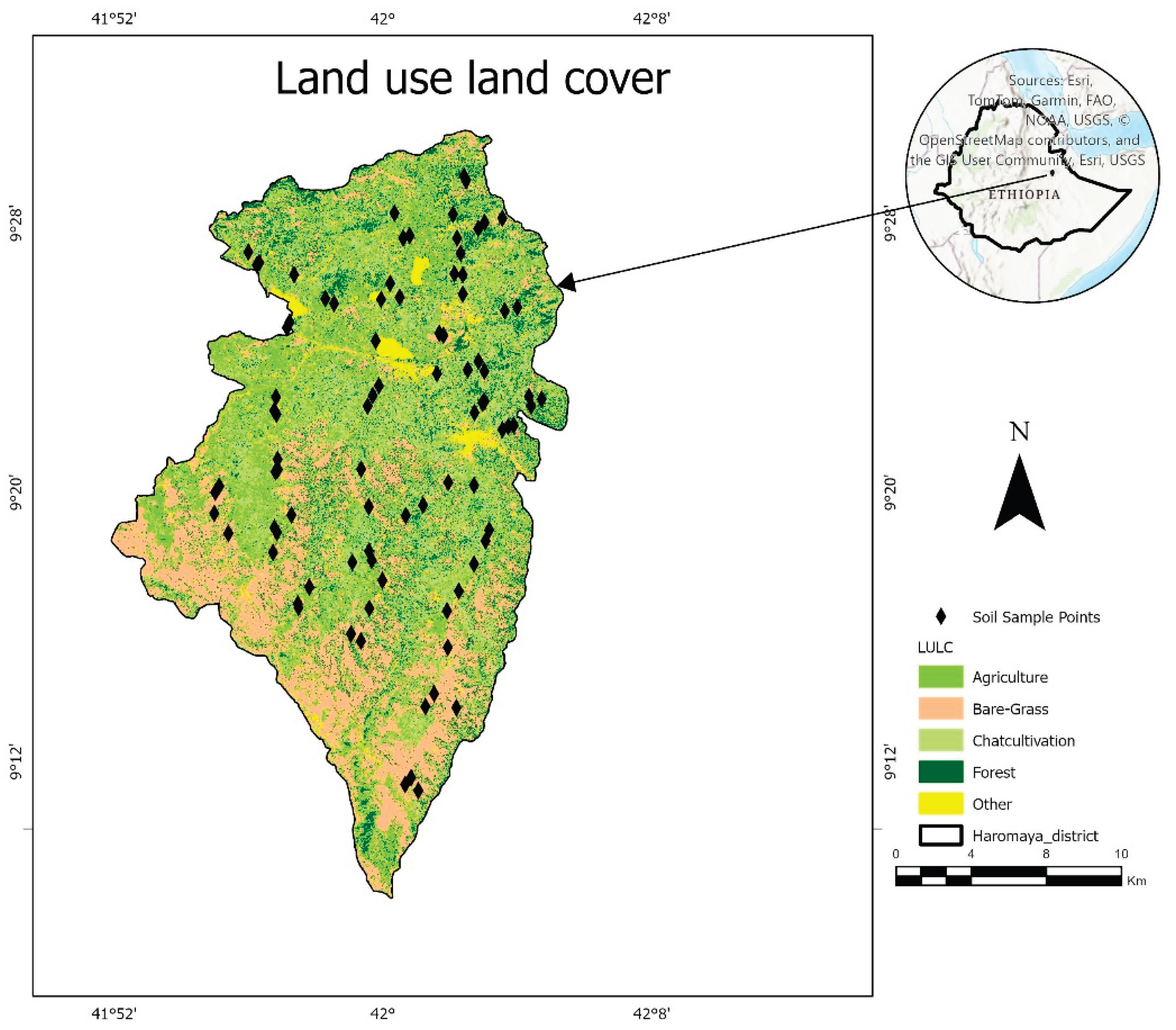
Figure 2.
Correlation of predictor indices derived from satellite image and environmental factors: (a)RapidEye, (b) Sentinel-2.
Figure 2.
Correlation of predictor indices derived from satellite image and environmental factors: (a)RapidEye, (b) Sentinel-2.
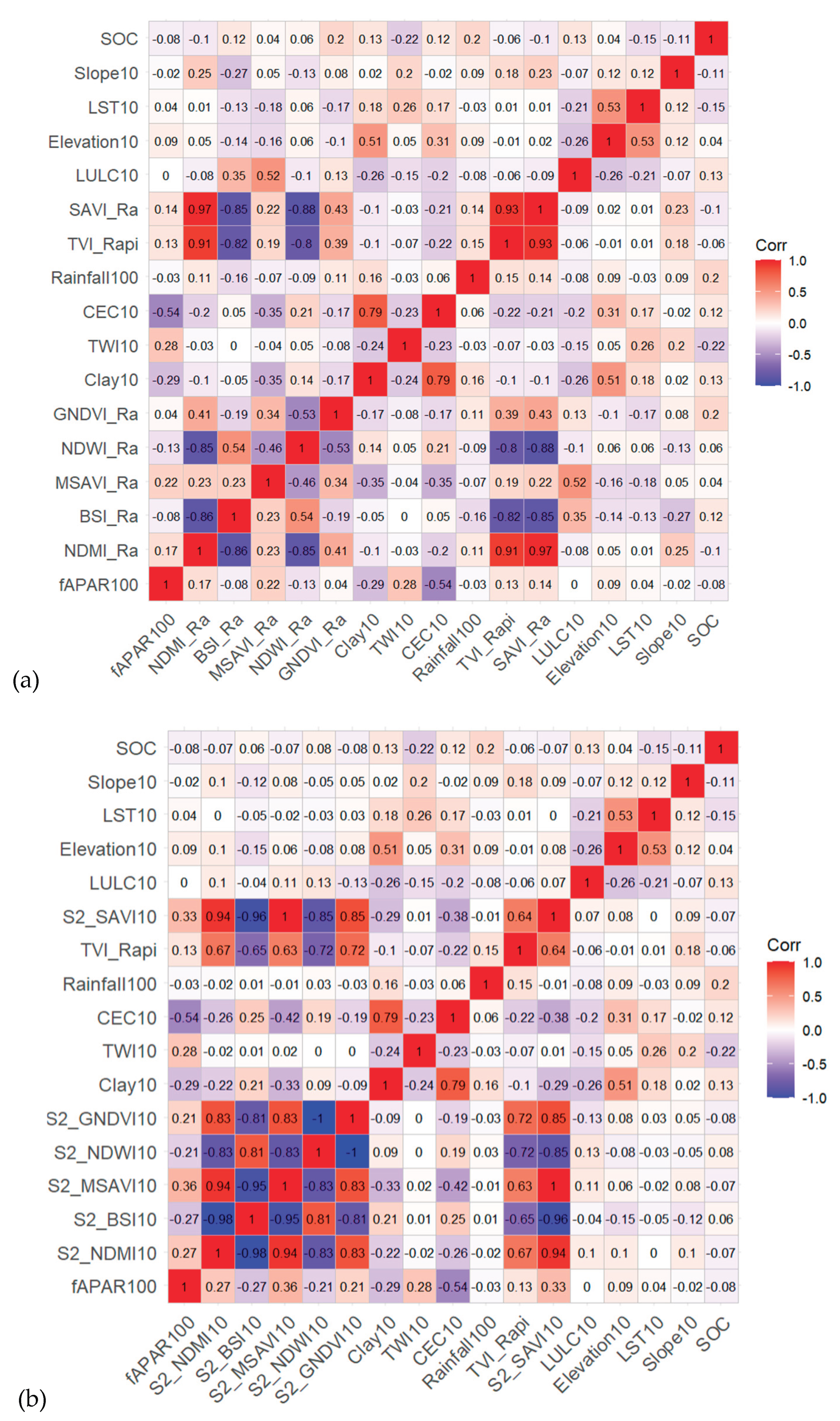
Figure 3.
RF based Actual vs Predicted SOC scatterolots from RapidEye (top) and Sentinel-2 (bottom).
Figure 3.
RF based Actual vs Predicted SOC scatterolots from RapidEye (top) and Sentinel-2 (bottom).

Figure 4.
Variable importance based on the RF model, RapidEye (top), Sentinel-2) (bottom).
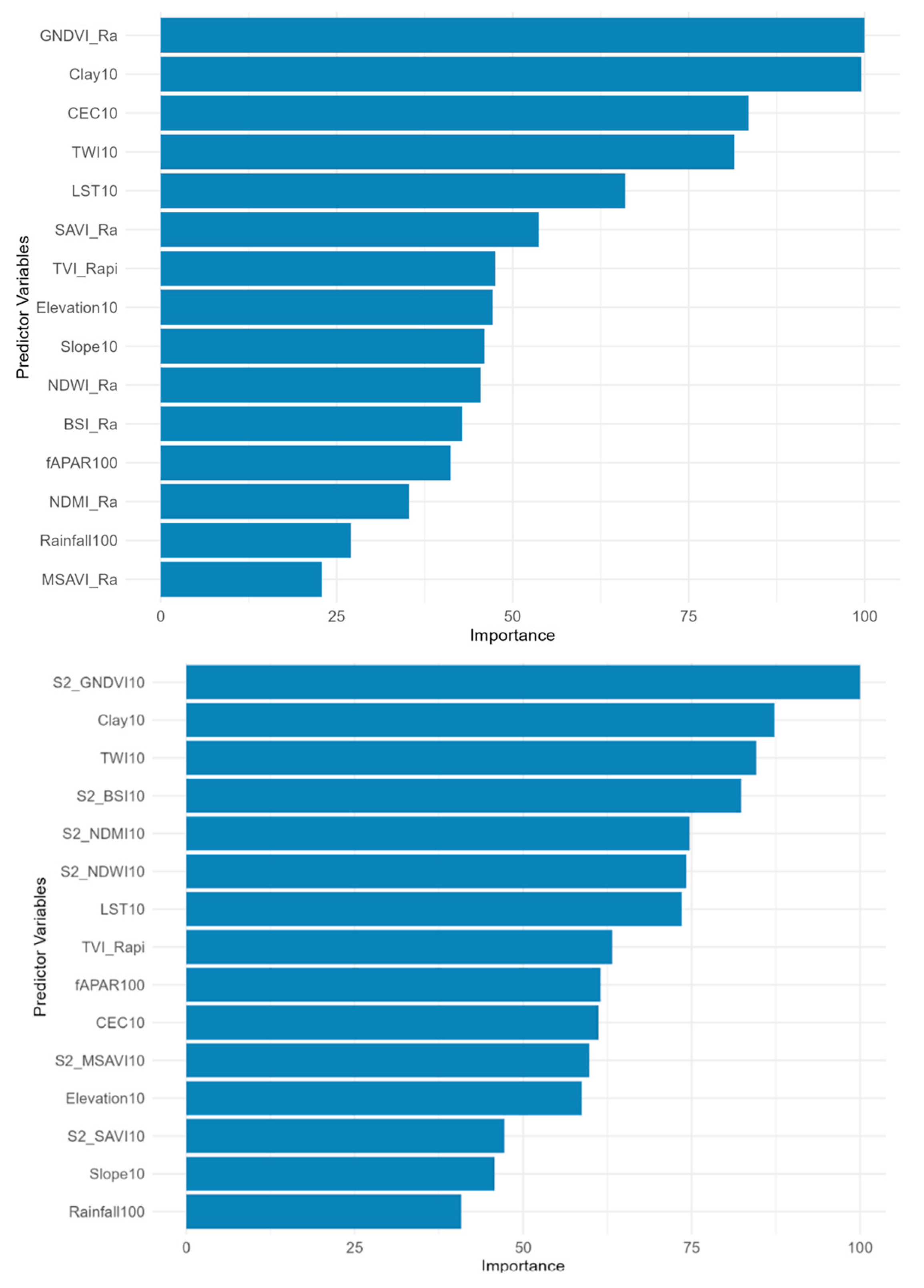
Figure 5.
Spatial map of SOC from RapidEye (Top) and Sentinel-2 (Bottom).
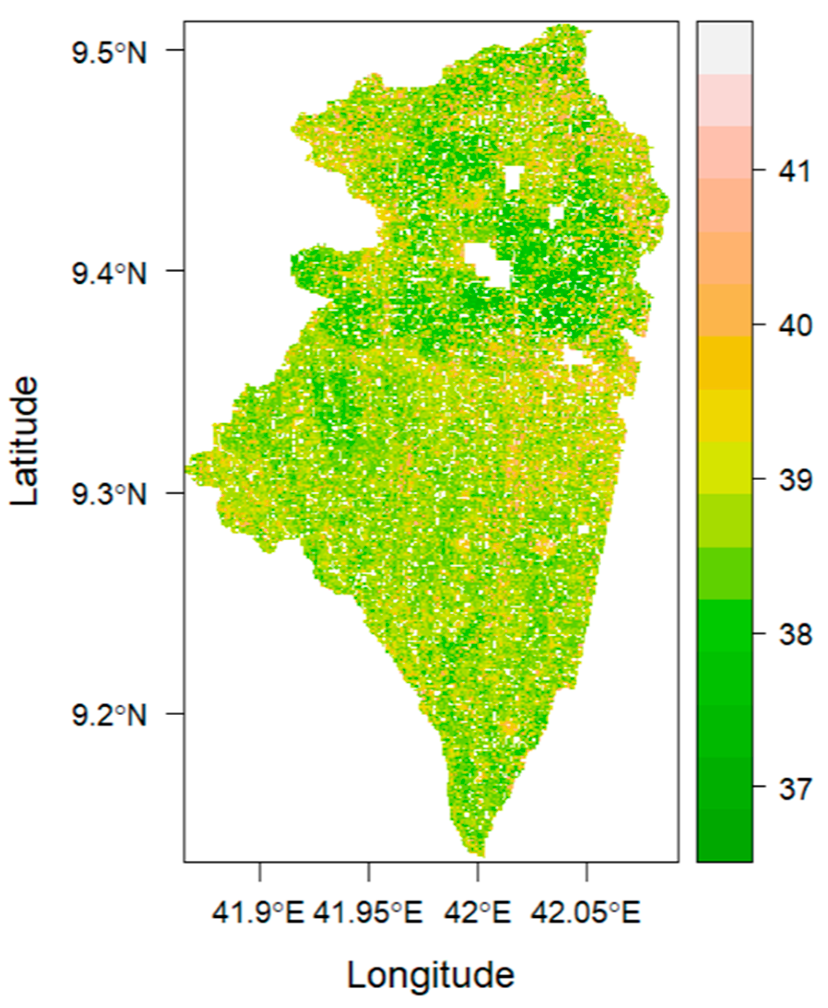
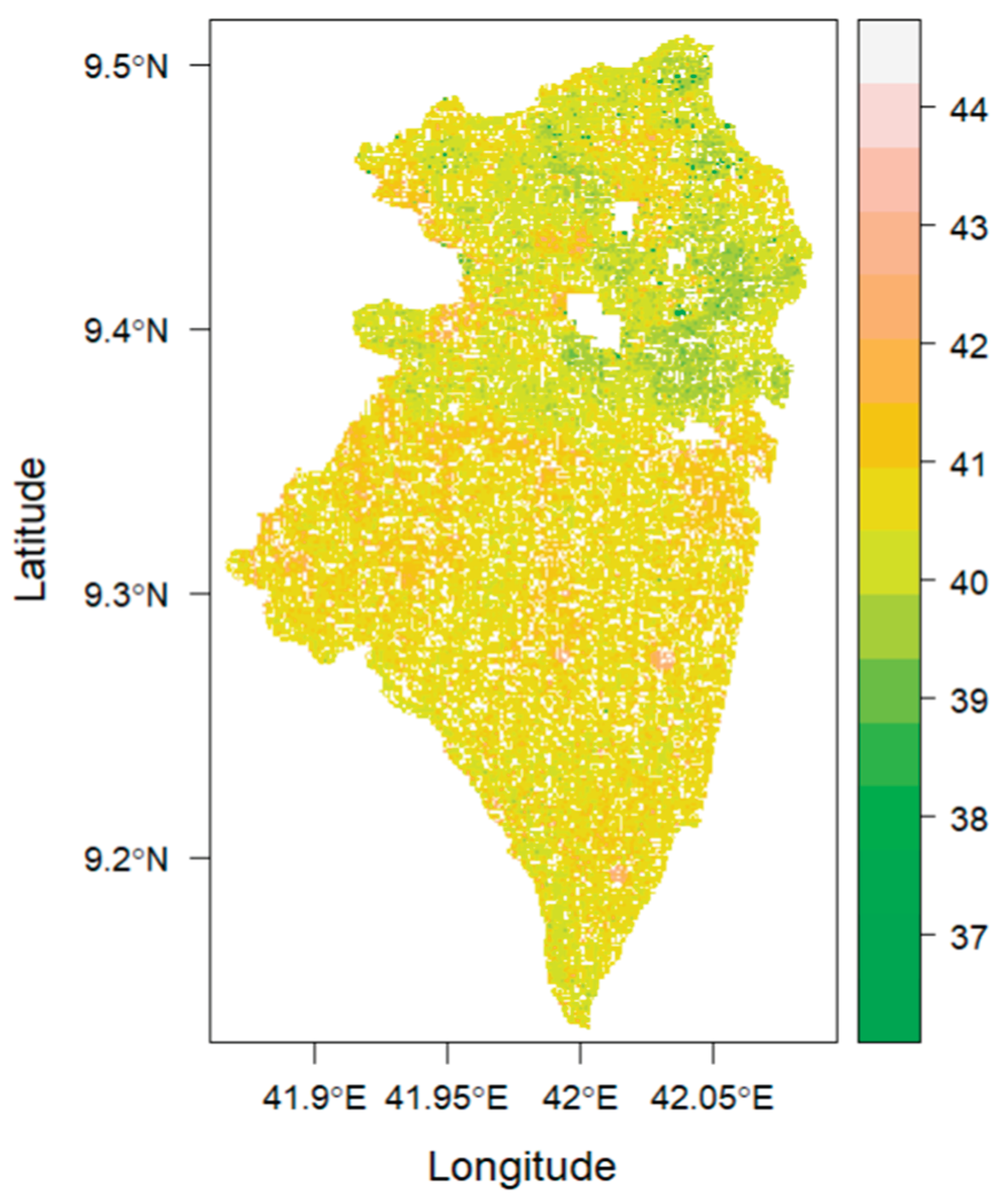

Table 1.
Spectral indices and their description of the equation.
| Indices | Description and Equation | References |
|---|---|---|
| MSAVI | Modified Soil Adjusted Vegetation Index 2NIR+1−sqr((2NIR+1)2−8(NIR−RED))/2 |
[43] |
| GNDVI | Green Normalized Difference Vegetation Index GNDVI=NIR-Green/NIR+Green, |
[44] |
| BSI | Bare Soil Index BSI=(Red+SWIR)-(NIR+Blue)/(Red+SWIR)+(NIR+Blue) |
[45] |
| NDMI | Normalized Difference Moisture Index NDMI=NIR+SWIR/NIR−SWIR |
[46] |
| SAVI | Soil Adguested Vegetaion Index SAVI= (NIR-R)/(NIR+R+L) ×(1+L), where L=0.5 |
[47] |
| NDWI | Normalized Difference Water Index NDWI = (Green – NIR)/(Green + NIR) |
[48] |
| TVI | Transformed Vegetaion Index TVI = Sqrt (NIR-Red/NIR+Red)+0.5 |
[35] |
Table 2.
lists the input variables used in this study.
| Sources | Typical Resolution (resampled to 5- and 10m) | Variables |
|---|---|---|
| MODIS | 500m(fAPAR),1km(LST) | fAPAR, LST |
| ASTER GDEM | 30m | Elevation, Slope, TWI |
| ISRIC SoilGrids | 250m | Sand, Clay, CEC |
| Field | 5 and 10m | Bulk Density (Interpolation) |
| CHIRPS | 0.05° (~5 km) | Rainfall |
| RapidEye | 5m | MSAVI, GNDVI, NDMI, BSI, SAVI, TVI, NDWI |
| Sentinel-2 | 10m | MSAVI, GNDVI, NDMI, BSI, SAVI, TVI, NDWI |
Table 3.
Statistics of LULC distribution in Haramaya district.
| LULC Types | Area in ha | Area in % |
| Agriculture | 15141.72 | 26.81% |
| Khat-cultivation | 15068.65 | 26.68% |
| Forest | 8004.95 | 14.18% |
| Bare-Grass-Shrub | 15510.27 | 27.47% |
| Other | 2744.61 | 4.86% |
| Total | 56470.2 | 100% |
Table 4.
Statistics for laboratory-measured soil bulk density (g/cm3) and OC value (%).
| Parameters | n | min | max | std.e | stdv | variance | Mean |
| BD | 88 | 0.978 | 1.77 | 0.018 | 0.167 | 0.028 | 1.356 |
| OC | 88 | 0.883 | 3.9 | 0.046 | 0.430 | 0.185 | 1.388 |
Table 5.
SOC computed per land use class/types in mg/ha RapidEye and Sentinel-2 data.
| RapidEye | Sentinel-2 | |||||||||||
| LULC | min | max | range | mean | std | min | max | range | mean | std | ||
| Agriculture | 36.7 | 41.9 | 5.2 | 38.6 | 0.6 | 36.3 | 44.2 | 7.9 | 40.6 | 0.5 | ||
| Khat-cultivation | 36.4 | 41.9 | 5.5 | 38.7 | 0.7 | 36.3 | 43.8 | 7.4 | 40.5 | 0.5 | ||
| Forest | 36.5 | 42.0 | 5.5 | 38.9 | 0.8 | 36.0 | 43.8 | 7.8 | 40.4 | 0.6 | ||
| Bare-Grass-Shrub | 36.6 | 41.7 | 5.1 | 38.7 | 0.5 | 36.5 | 44.8 | 8.2 | 40.7 | 0.5 | ||
Disclaimer/Publisher’s Note: The statements, opinions and data contained in all publications are solely those of the individual author(s) and contributor(s) and not of MDPI and/or the editor(s). MDPI and/or the editor(s) disclaim responsibility for any injury to people or property resulting from any ideas, methods, instructions or products referred to in the content. |
© 2025 by the authors. Licensee MDPI, Basel, Switzerland. This article is an open access article distributed under the terms and conditions of the Creative Commons Attribution (CC BY) license (http://creativecommons.org/licenses/by/4.0/).
Copyright: This open access article is published under a Creative Commons CC BY 4.0 license, which permit the free download, distribution, and reuse, provided that the author and preprint are cited in any reuse.


